KDLSQ-BERT: A Quantized Bert Combining Knowledge Distillation with Learned Step Size Quantization

Abstract

Recently, transformer-based language models such as BERT have shown tremendous performance improvement for a range of natural language processing tasks. However, these language models usually are computation expensive and memory intensive during inference. As a result, it is difficult to deploy them on resource-restricted devices. To improve the inference performance, as well as reduce the model size while maintaining the model accuracy, we propose a novel quantization method named KDLSQ-BERT that combines knowledge distillation (KD) with learned step size quantization (LSQ) for language model quantization. The main idea of our method is that the KD technique is leveraged to transfer the knowledge from a ”teacher” model to a ”student” model when exploiting LSQ to quantize that ”student” model during the quantization training process. Extensive experiment results on GLUE benchmark and SQuAD demonstrate that our proposed KDLSQ-BERT not only performs effectively when doing different bit (e.g. 2-bit $\sim$ 8-bit) quantization, but also outperforms the existing BERT quantization methods, and even achieves comparable performance as the full-precision base-line model while obtaining 14.9x compression ratio. Our code will be public available.

1 Introduction

Recently, transformer-based language models such as BERT Devlin et al. (2018) and RoBertaLiu et al. (2019) have achieved remarkable performance on many natural language processing tasks. However, it is difficult to deploy these models on resource-restricted devices directly since they usually contain lots of weight parameters that are computation expensive and memory intensive. To alleviate this problem, many various approaches have been widely explored to compress the model size. For instance, low-rank approximation Ma et al. (2019), Lan et al. (2019), weight-sharing Dehghani et al. (2018), Lan et al. (2019); knowledge distillation Sanh et al. (2019),Sun et al. (2019), Jiao et al. (2019); pruning Michel et al. (2019), Voita et al. (2019), Fan et al. (2019); dynamic network training Liu et al. (2019), Hou et al. (2020) and quantization Zafrir et al. (2019), Shen et al. (2020), Fan et al. (2020), Krishnamoorthi (2018), etc.

Compared with other compression methods, quantization is widely used to compress neural network models due to two main reasons. First, quantization is an important technique enabling low-power and high-throughput DNN inference, especially it is hardware-friendly for the inference on those the resource-restricted devices such as cell-phones. Second, quantization does not change the model architecture, thus it is particularly useful for the carefully-designed network such as Transformers Vaswani et al. (2017). Furthermore, 8-bit quantization is successfully applied to Transformer-based models since it can achieve a comparable performance as the full-precision baseline Prato et al. (2019), Zafrir et al. (2019). However, it is challenging to quantize these models within ultra low-bit (e.g., 2-bit) because of the dramatically accuracy dropping. To alleviate this issue, many complex quantization methods are proposed, mainly including mixed-precision quantization Shen et al. (2020), Zadeh & Moshovos (2020), product quantization (PQ) Fan et al. (2020), and ternary quantization Zhang et al. (2020). However, different quantization methods include different features: mixed-precision quantization is not always hardware-friendly, PQ needs extra clustering operations during the training process, and ternary quantization is not a generative method that focus only on 2-bit quantization rather than on arbitrary bit quantization.

In addition to quantization, knowledge distillation (KD) Hinton et al. (2015) is another widely used compression method in which a compact model (”student”) is trained to reproduce the behaviour of a larger model (”teacher”). For natural language processing tasks, KD has been extensively studied Hu et al. (2018), Jiao et al. (2019). However, instead of being used to compress models individually, KD also can be exploited by combining with other compression techniques McCarley (2019), Zhang et al. (2020), Hou et al. (2020), Mao et al. (2020).

In this work, we propose a novel BERT quantization algorithm named KDLSQ-BERT that even can achieve high accuracy via doing ultra low-bit (e.g. 2-bit) quantization. The main idea of our method is that the KD technique is leveraged to transfer the knowledge from a ”teacher” BERT to a ”student” one when exploiting learned step size quantization (LSQ) Esser et al. (2019), Jain et al. (2019) to quantize that ”student” BERT during the quantization training process. More specifically, the contributions of our work can be summarized as follows:

• Inspired by Jiao et al. (2019), we use KD to transfer the knowledge from a full-precision ”teacher” BERT to a quantized ”student” BERT. The distillation loss in our work is calculated by the corresponding layers (such as the embedding layers and the outputs of Transformer layers) from the ”teacher” BERT and the quantized ”student” BERT, respectively.

• Due to the excellent performance of LSQ in low-bit quantization in computer vision field Jain et al. (2019), we introduce such a technique to quantize the ”student” BERT. To accelerate the quantization training speed and improve the model accuracy, however we present a novel method to initialize the correlated scale-factors. Furthermore, it’s easy for user to fine-tune the LSQ quantization training when using such an initialization method.

• In fact KD can be more useful to train a ”student” model only if the ”teacher” model is well trained. It figures out that the distillation loss cannot work well if the ”teacher” model is not well trained enough. As such, we introduce the ground truth loss built by the training data to compute the backward gradients during the training process. The extensive experiments show that the accuracy of quantized BERT can obtain a remarkable improvement if applying both distillation loss and ground truth loss.

The main work of this paper is organized as follows: The related work regarding knowledge distillation and quantization for BERT is introduced in Section 2; The main idea of our work is presented in Section 3; In Section 4, we do extensive experiments as well as the relevant result analysis; Finally, we summarize our work and point out the future work in Section 5.

2 Related Work

2.1 Knowledge Distillation

As a widely used compression technique, KD Hinton et al. (2015) aims at transferring the knowledge from a larger model (”teacher”) to a compact model (”student”) without sacrificing too much performance. Recently, many studies reveal that KD can achieve remarkable performance in a range of NLP tasks Kim & Rush (2016), Jiao et al. (2019). Especially, for KD on BERT compression, more comprehensive knowledge including logits, intermediate representations and attentions are adopted to train the student BERT Jiao et al. (2019), Wang et al. (2020), Romero et al. (2014).

Besides, many studies show that for further model compression, KD is usually used to work with other compression techniques such as pruning McCarley (2019), low-rank approximation Mao et al. (2020) and dynamic networks training Hou et al. (2020). To do so, the knowledge of the teacher BERT model can be fully leveraged, so that the student BERT can get more remarkable compression or accuracy performance improvement.

However, it should be noted that combining KD with quantization could be a promising technique for model compression as the quantized student model not only can improve the accuracy through knowledge transferring, but also can be hardware-friendly for inference. And, many related studies have been explored in convolutional neural networks (CNNs) models Polino et al. (2018), Stock et al. (2019), Kim et al. (2019). Although TernaryBERT Zhang et al. (2020) is designed based on KD along with quantization, such a method mainly provides 2-bit and 8-bit weight quantization rather than arbitrary bit quantization. As a result, here we make our efforts to exploit KD and quantization to explore more general method for Transformer-based model quantization.

2.2 Quantization

Recently, quantization training has been extensively studied since the quantized models can gain a significant accuracy compensate through training process. The studies of Quantization-Aware Training (QAT) Jacob et al. (2018) and Training Quantization Thresholds (TQT)Esser et al. (2019), Jain et al. (2019) indicate that compared to the full-precision CNN model, the corresponding quantized model can obtain a slight accuracy drop (smaller than 1.0%) when doing 8-bit quantization training. Besides, for the Transformers-based models, 8-bit quantization training is also successfully applied in fully quantized Transfomer (FullyQT) for machine translation Prato et al. (2019) and Q8BERT Zafrir et al. (2019). Note that FullyQT and Q8BERT are designed based on QAT, the experimental results from Prato et al. (2019) and Zhang et al. (2020) show that FullyQT and Q8BERT do not work well in low-bit (e.g., 2 bit or 4-bit) quantization.

In addition, many studies has been investigated in low bit quantization for the Transformers-based models. For instance, Q-BERT Shen et al. (2020) achieves ultra-low bit quantization in terms of the analysis of fine-tuned BERT using the second order Hessian information. To avoid severe accuracy drop, mixed-precision with 3 or more bits are exploited in Q-BERT. In this case, it is usually un-friendly for inference to some hardware even though the accuracy of the quantized BERT can be enhanced to some extent. Quant-Noise (QN) Fan et al. (2020) is proposed to quantize a subset of weights in each iteration to allow unbiased gradients to flow through the model architecture. Although the high compression rate can be achieved, the quantization noise rate needs to be very carefully tuned for good performance. For TernaryBERT Zhang et al. (2020), it is mainly used to quantize the different parts of the BERT model through 2-bit ternarization training. To avoid the accuracy drop caused by 2-bit ternarization, various distillation losses are considered to guide the quantization training process.

In this work, we extend LSQ to quantize Transformers-based models such as BERT, because the results in Esser et al. (2019) reveal that such a quantization method is competitive in low-bit quantization for CNN models. To guarantee the accuracy of the quantized model as well as accelerate the training convergence, in our work we not only propose a novel scale-factor initialization for LSQ, but also consider various losses (including various distillation losses and ground truth loss) to guide the quantization training process.

3 Methodology

In this section, we make our efforts to combine knowledge distillation with LSQ to quantize BERT. Different from the previous work Zhang et al. (2020) and Jacob et al. (2018), our method has much broader capacity in different bit quantization, meaning that it can be used not only in low-bit (e.g., 2-bit) quantization but also in high-bit (e.g., 8-bit) quantization. The main quantization training framework of our method is described in Figure 1. On the one hand, the LSQ quantization operations (see equation 6) need to be inserted into the student model already when doing quantization training. Note that the tensors that need to be quantized include weights as well as the inputs of all linear layers and matrix multiplications. On the other hand, the total loss $Loss_{total}$ (see equation 15) is calculated based not only on the teacher model, but also on the ground truth from the training data set. Of course, the ground truth loss $Loss_{gt}$ (see equation 15) can be optional if the teacher model is well-trained. This is because the distillation loss $Loss_{kd}$ (see equation 14) is enough for the student model to do quantization training if a well-trained teacher is provided. For more details on our proposed method, please see the next further discussion.

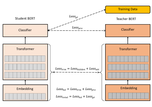
Figure 1: The training framework of our proposed KDLSQ-BERT. In fact, the student BERT is inserted into LSQ quantization operations already after the training framework is built. The distillation loss $Loss_{kd}$ related to the knowledge of teacher BERT includes the hidden-states-based distillation loss $Loss_{hidden}$, the attention-based distillation loss $Loss_{att}$, as well as the prediction-layer-based distillation loss $Loss_{pre}$.

3.1 Transformer Layer

Most of the recent language models (e.g., BERT Devlin et al. (2018), XLNet Yang et al. (2019), RoBerta Liu et al. (2019) and TinyBert Jiao et al. (2019)) are built with several Transformer layers, the main feature of which is to capture long-term dependencies between input tokens by self-attention mechanism. A standard Transformer layer includes two main sub-layers: Multi-Head Attention (MHA) and fully connected Feed-Forward Network (FFN).

For the $l$-th Transformer layer, assuming its input is $\mathbf{H}_{l}\in\mathbb{R}^{n\times d}$, where $n$ and $d$ denote the sequence length and hidden state size, respectively. Besides, suppose there are $N_{H}$ attention heads in each Transformer layers, and head $h$ is parameterized by $\mathbf{W}^{Q}_{h},\mathbf{W}^{K}_{h},\mathbf{W}^{V}_{h},\mathbf{W}^{O}_{h}\in\mathbb{R}^{d\times d_{h}}$, where $d_{h}=\frac{d}{N_{H}}$. Then the output of head $h$ can be denoted as:

$$\textrm{head}_{h}(\mathbf{H}_{l})=\textrm{Softmax}(\frac{1}{\sqrt{d}}\mathbf{H}_{l}\mathbf{W}^{Q}_{h}\mathbf{W}^{K\top}_{h}\mathbf{H}^{\top}_{l})\mathbf{H}_{l}\mathbf{W}^{V}_{h}$$ (1)

Let $\mathbf{W}^{*}=[\mathbf{W}^{*}_{1},...,\mathbf{W}^{*}_{N_{H}}]$, where $*$ could be anyone of $Q$, $K$ and $V$, then the output of MHA is calculated by:

$$\textrm{MHA}_{\mathbf{W}^{Q},\mathbf{W}^{K},\mathbf{W}^{V},\mathbf{W}^{O}}(\mathbf{H}_{l})=\textrm{Concat}(\textrm{head}_{1},...,\textrm{head}_{N_{H}})\mathbf{W}^{O}$$ (2)

Suppose two linear layers in FFN are parameterized by $\mathbf{W}^{1}\in\mathbb{R}^{d\times d_{ff}}$, $\mathbf{b}^{1}\in\mathbb{R}^{d_{ff}}$ and $\mathbf{W}^{2}\in\mathbb{R}^{d_{ff}\times d}$, $\mathbf{b}^{1}\in\mathbb{R}^{d}$ respectively, where $d_{ff}$ indicates the number of neurons in the intermediate layer of FFN. Meanwhile, let $\mathbf{X}_{l}\in\mathbb{R}^{n\times d}$ denote the input of FFN, the corresponding output is then computed as:

$$\textrm{FFN}(\mathbf{X}_{l})=\textrm{GeLU}(\mathbf{X}_{l}\mathbf{W}^{1}+\mathbf{b}^{1})\mathbf{W}^{2}+\mathbf{b}^{2}$$ (3)

Using equation 2 and equation 3, the forward propagation for the $l$-th Transformer layer can be written as:

$$\mathbf{X}_{l} =\textrm{LN}(\mathbf{H}_{l}+\textrm{MHA}(\mathbf{H}_{l}))$$ (4)

$$\mathbf{H}_{l+1} =\textrm{LN}(\mathbf{X}_{l}+\textrm{FFN}(\mathbf{X}_{l}))$$

where LN is the layer normalization. Note that the input $\mathbf{H}_{1}$ for the first Transformer layer is from the embedding layer, so it can be denoted as:

$$\mathbf{H}_{1}=\textrm{EMB}_{\mathbf{W}^{E},\mathbf{W}^{S},\mathbf{W}^{P}}(\mathbf{z})$$ (5)

where $\mathbf{z}$ is the input sequence, and $\mathbf{W}^{E},\mathbf{W}^{S}$ and $\mathbf{W}^{P}$ are the learnable word embedding, segment embedding and position embedding, respectively.

3.2 Learned Step Size Quantization for BERT

Typically, model quantization is useful for inference acceleration because of less computing-resource consumption of the low precision integer operations. Inspired by Esser et al. (2019), here we explore to quantize BERT by LSQ, the basic feature of which is that the scale-factors can be learned during the quantization training process. Specifically, the basic equations for quantization and de-quantization on LSQ are as follows:

$$q_{v} =\textrm{round}(\textrm{clamp}(\frac{v}{s},-Q_{n},Q_{p}))$$ (6)

$$\hat{v} =q_{v}\times s$$

where $\textrm{clamp}(z,r_{1},r_{2})=\textrm{min}(\textrm{max}(z,r_{1}),r_{2})$, $v$ is a real number that needs to be quantized, $q_{v}$ is the quantized integer number of $v$, $s$ denotes the scale-factor, $\hat{v}$ is the de-quantization result, and $Q_{n}$ and $Q_{p}$ are the negative and positive quantization levels respectively. Given a bit number $b$ for quantization, then for unsigned tensor (e.g., activations), $Q_{n}=0$ and $Q_{p}=2^{b}-1$; for signed tensor (e.g., weights), $Q_{n}=2^{b-1}-1$ and $Q_{p}=2^{b-1}-1$. Consequently, LSQ can be considered as a symmetric quantization.

Note that LSQ provides a way to learn $s$ in term of the training loss, then in terms of equation 6, the gradient to $s$ can be calculated as:

$$\frac{\partial\hat{v}}{\partial s}=\left\{\begin{array}[]{lll}-\frac{v}{s}+\textrm{round}(\frac{v}{s})&\textrm{if}&-Q_{n}<\frac{v}{s}<Q_{p}\\ -Q_{n}&\textrm{if}&\frac{v}{s}<-Q_{n}\\ Q_{p}&\textrm{if}&\frac{v}{s}>Q_{p}\end{array}\right.$$ (7)

With STE Bengio et al. (2013), the gradient through the quantization function for activations can be approximated by:

$$\frac{\partial\hat{x}}{\partial x}=\left\{\begin{array}[]{ll}1&\textrm{if}-Q_{n}<\frac{x}{s}<Q_{p}\\ 0&\textrm{otherwise}\end{array}\right.$$ (8)

To avoid weights becoming permanently stuck in the clipped range, however, the gradient through the quantization function for weights is computed as:

$$\frac{\partial\hat{w}}{\partial w}=1$$ (9)

For weight quantization, we follow the analysis from Zhang et al. (2020) and Zafrir et al. (2019) to quantize weights $\mathbf{W}^{Q},\mathbf{W}^{K},\mathbf{W}^{V},\mathbf{W}^{O}$ from all transformer layers, as well as the word embedding $\mathbf{W}^{E}$. However, we do not implement quantization on $\mathbf{W}^{S}$ and $\mathbf{W}^{P}$ from the embedding layer, as well as the bias in linear layers because of two reasons. First, the number of these weights is negligible, thus it has less impact on the quantized model size even if quantizing them. Second, some of them contain critical information (e.g., the position information in $\mathbf{W}^{P}$ affects the dependency for each word) that results in significantly accuracy dropping if they are quantized. Similar to work done by Zhang et al. (2020), softmax operation, layer normalization and the last task-specific layer are not quantized in our work. This is because quantizing these operations will lead to accuracy degradation dramatically.

With regards to the activation quantization, the inputs of all linear layers and matrix multiplication in Transformer layers are quantized. In fact, it is a symmetric quantization, so that the quantized values distribute symmetrically in both sides of 0. That is, the zero point is 0, which is benefit to accelerate inference of the quantized model.

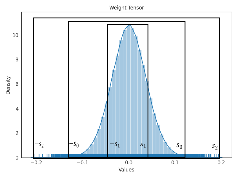
Figure 2: The statistical histogram of a weight tensor from a well-trained TinyBERT. Compared with $s_{1}$ and $s_{2}$, $s_{0}$ is a much better initialized scale-factor (or truncated threshold) for quantization training since the main information of the weight tensor can be retained.

However, we cannot expect a promising quantization result if the scale-factor $s$ for LSQ are not initialized effectively. In essence, the scale-factor can be considered as a truncated threshold for a tensor that needs to be quantized. To analyze its importance, Figure 2 presents the relationship between different scale-factors and the statistical histogram of a weight tensor from a well-trained TinyBERT. As illustrated in the figure, $s_{0}$ is a much better initialization than $s_{1}$ and $s_{2}$ since most parts of the tensor are retained by using $s_{0}$. In contrast, if using $s_{1}$, only a few parts of that tensor are retained, so that main information of that tensor will be lost. Obviously, if $s_{2}$ is employed, lots of boundary elements that are not in the main distribution of that tensor will be kept for quantization. In this case, such invalid information must result in accuracy dropping especially when doing low-bit quantization. Many readers may have a question that scale-factor will be updated as the training goes on, why shouldn’t the scale-factor be initialized randomly? Indeed, although the scale-factor changes during the training process, an effective initialization is good to accelerate the loss convergence, as well as improve the model accuracy. Particularly, it will lead to difficult convergence for low-bit LSQ quantization training when the scale-factor is not effectively initialized.

To alleviate aforementioned issue, we propose a method to initialize the scale-factor for a given tensor that needs to be quantized. The main steps for the method are listed as follows:

Algorithm 1 A method to initialize scale-factor

0:  A given tensor $M$, a truncated ratio $\gamma$

0:  An initialized scale-factor $s_{init}$

1:  $n=\textrm{nelement}(M)$, where $n$ is the number of elements in $M$.

2:  $M_{sort}=\textrm{Sort}(M)$, where $M_{sort}$ is a sorted $M$ in ascending order.

3:  $\textrm{index}_{min}=\textrm{round}(\frac{\gamma\times n}{2})$

4:  $\textrm{index}_{max}=n-\textrm{index}_{min}$

5:  if $\textrm{abs}(M_{sort}(\textrm{index}_{min}))\geq\textrm{abs}(M_{sort}(\textrm{index}_{max}))$ then

6:     $s_{init}=\textrm{abs}(M_{sort}(\textrm{index}_{min}))$

7:  else

8:     $s_{init}=\textrm{abs}(M_{sort}(\textrm{index}_{max}))$

9:  end if

10:  return  $s_{init}$

From algorithm 1, it shows that the truncated ratio $\gamma$ (where $\gamma\ll 1$) determines how many elements in $M$ need to be truncated. With $\gamma$ and the sorted $M_{sort}$, $s_{init}$ is initialized to a value that can be regarded as a threshold for truncation. More specifically, the elements that are greater than $s_{init}$ need to be truanted to $Q_{p}$, the elements that are smaller than $-s_{init}$ need to be truanted to $-Q_{n}$, so the most of elements in a range of $(-s_{init},s_{init})$ are not changed. That’s, since the elements in $M$ are truanted in terms of $s_{init}$, the majority information of $M$ can be retained for quantization.

As analyzed previously, both weights and activations need to be quantized by LSQ. For weights, we make use of the corresponding weight values from the full-precision BERT to do scale-factor initialization. Of course, the full-precision BERT should be well trained and be set as a pre-trained model for LSQ quantization training. For activations, however, it is a little bit different as activations cannot be obtained from the full-precision BERT directly. Therefore, we leverage a batch of training data set (which is selected randomly) to do inference for the full-precision BERT, such that the correlated activations can be obtained. After the activations are calculated, the related scale-factors can be initialized according to Algorithm 1.

3.3 Distillation-Aware Quantization

For quantization training, although the model accuracy loss introduced by quantization can be compensated through training process, it may be less effective when doing low-bit quantization. To address such a problem, thus we take advantage of KD to further improve the accuracy performance of the quantized BERT. Following the teacher-student KD framework, we set the quantized BERT and the well-trained full-precision BERT to be the student model and the teacher model, respectively. For the quantized BERT, the related LSQ quantization operations are inserted already, and it can learn to recover the behaviours of the teacher model via the KD technique.

Inspired by Zhang et al. (2020) and Jiao et al. (2019), the distillation loss for the Transformer layers mainly relies on the outputs of all Transformer layers, the outputs of embedding layer, as well as the attention scores of all heads from all Transformer layers. More specifically, considering the outputs of all Transformer layers and the outputs of embedding layer, the hidden-states-based distillation loss $Loss_{hidden}$ can be calculated as follows:

$$Loss_{hidden}=\sum_{l=1}^{L+1}\textrm{MSE}(\mathbf{H}_{l}^{S},\mathbf{H}_{l}^{T})$$ (10)

where MSE indicates the mean squared error, $L$ is the number of Transformer layers for BERT, $\mathbf{H}_{l}^{S}$ ($\mathbf{H}_{l}^{T}$) is the inputs of the $l$-th Transformer layer from the student model (teacher model). However, note that $\mathbf{H}_{L+1}^{S}$ ($\mathbf{H}_{L+1}^{T}$) denotes the outputs of the last Transformer layer from the student model (teacher model). For the attention-based distillation loss $Loss_{att}$ Clark et al. (2019) related to the attention scores of all heads from all Transformer layers, it can be computed by:

$$Loss_{att}=\sum_{l=1}^{L}\textrm{MSE}(\mathbf{A}_{l}^{S},\mathbf{A}_{l}^{T})$$ (11)

Consequently, the distillation loss $Loss_{trm}$ for all Transformer layers is computed by:

$$Loss_{trm}=Loss_{hidden}+Loss_{att}$$ (12)

In addition to Transformer layers, the knowledge from the prediction layer affects the accuracy performance significantly. Therefore, we also distill that knowledge, such that the logits $\mathbf{P}^{S}$ from the student model can learn to fit the corresponding $\mathbf{P}^{T}$ from the teacher model by soft cross-entropy (SCE) loss:

$$Loss_{pre}=\textrm{SCE}(\mathbf{P}^{S},\mathbf{P}^{T})$$ (13)

Consequently, the total distillation loss $Loss_{kd}$ established between the student model and the teacher model can be computed by:

$$Loss_{kd}=Loss_{pre}+Loss_{trm}$$ (14)

However, both theoretical and empirical discoveries show that $Loss_{kd}$ can work well for training only if the teacher model is well-trained. That’s, a bad teacher model results in a bad accuracy for the student model. To avoid the unexpected result caused by a bad teacher model, we introduce the ground truth loss $Loss_{gt}$ that needs to be calculated according to the label truth of the training data set. In doing so, the quantization training loss for the student model is not only related to the teacher model, but also related to the training data set. Thus, the total training loss can be computed by:

$$Loss_{total}=Loss_{kd}+Loss_{gt}$$ (15)

According to the analysis above, the whole procedure of our distillation-aware LSQ quantization can be summarized as follows:

Algorithm 2 KDLSQ-BERT: A novel distillation-aware quantization based on LSQ

0:  Training data set, A well-trained full-precision BERT.

0:  A quantized student BERT

1:  Initialize the teacher model and student model by the well-trained full-precision BERT.

2:  Initialize the scale-factors for the weights in student model in terms of Algorithm 1.

3:  Get activations by doing inference of the student model with a randomly selected batch of training data set.

4:  Initialize the scale-factors for the above activations (including the inputs of linear layers and the inputs of the matrix multiplications) in terms of Algorithm 1.

5:  Insert the LSQ quantization operations into the student model according to equation 6.

6:  Initialize the learning rate $\eta$ and $epochs$.

7:  for $i=1,...,epoches$ do

8:     for $iter=1,...,max_{batch}$  do

9:        Get the $iter$-th batch of training data set.

10:        Compute the loss according to equation 15.

11:        Compute the correlated gradients according to equation 7, equation 8, and equation 9.

12:        Update the weights and the scale-factors for the student model.

13:        Update the learning rate $\eta$.

14:     end for

15:  end for

4 Experimental Analysis

In this section, we main evaluate the performance of our proposed KDLSQ-BERT on both the GLUE benchmark Wang et al. (2018) and SQuAD Rajpurkar et al. (2016). The specific information for those data sets are listed as follows:

The GLUE benchmark: The GLUE benchmark is a collection of diverse natural language understanding tasks, including textual entailment (RTE), natural language inference (MNLI, QNLI), similarity and paraphrashe (MRPC, QQP, and STS-B), sentiment Analysis (SST-2) and linguistic acceptability (CoLA). For the performance evaluation metrics Chicco & Jurman (2020), we follow the work of TinyBERTJiao et al. (2019) by setting Matthews Correlation for CoLA, F1 for MRPC and QQP, Spearman Correlation for STS-B, and accuracy for the other tasks.

SQuAD: SQuAD v1.1 is a machine reading comprehension task. Given a question-passage pair, the task is to extract the answer span from the passage. SQuAD v2.0 is a updated version in which the question might be unanswerable. For the performance evaluation metric Derczynski (2016), also we follow the work of TinyBERTJiao et al. (2019) by considering F1 for these two data sets.

In addition, the code for our proposed method is modified from the huggingface pytorch-transformer library, Q8BERT and TinyBERT. To effectively investigate the performance of our method, we set Q8BERT Zafrir et al. (2019) and TernaryBERT Zhang et al. (2020) as the comparison methods. For Q8BERT, we set arbitrary bit (2-bit $\sim$ 8-bit) weight quantization as well as the fixed 8-bit activation quantization for fair comparison. For TernaryBERT, we consider 2-bit and 8-bit weight quantization for comparison according to the discussion did by Zhang et al. (2020). However, we do not use Q-BERT Shen et al. (2020) as a comparison algorithm since it is not open-source. Here we abbreviate the quantization bit for weights of Transformer layers, word embedding and activations as ”W-E-A (#bit)”. If not specified, ”W-E-A (#bit)” denotes the same meaning for our next experimental analysis. The used BERT models in our experiments include TinyBERT and BERT-base, and the specific information of these models are listed in Table 1.

Table 1: The basic information for the used BERT models

Model	Transformer	Hidden	Feed-Forward	Model
	Layers	Size	Size	Size(MB)
BERT-base	12	768	3072	418 ($\times 1$)
TinyBERT	6	768	3072	258 ($\times 1.6$)

For the truncated ratio $\gamma$ which is the input of Algorithm 1, we set it to be $0.05$ , meaning that a tensor that needs to be quantized can be retained $95.0\%$ information for quantization. However, the initial learning rate for weight scale-factors is different from that for activation scale-factors. For weight scale-factors, we set the corresponding initial learning rate to be $1.0\times 10^{-3}$ since a well-trained pre-trained model can provide effective weight parameters for scale-factor initialization. In doing so, the small initial learning rate can bring small update size, so that the weight scale-factors can be updated slightly during the quantization training process. Differently, as the activations are estimated by a batch size of training data, such an inaccurate estimation requires that the initial learning rate of activation scale-factors should be greater than that of weight scale-factors. Therefore, we set the initial learning rate for activation scale-factors to be $2.0\times 10^{-2}$, so that the corresponding scale-factors can be updated effectively. Besides, the learning rate is set to decay linearly to 0 during the quantization training, and the number of training epoch is set to be 3.0.

4.1 Experimental Comparison with Existing BERT Quantization Methods

For the GLUE benchmark, we conduct the experiments with the batch size of 16 for CoLA and 32 for other tasks. The learning rate is initialized to $2\times 10^{-5}$ and decays linearly to 0 during 3.0 training epochs. The maximum sequence length is 64 for single-sentence tasks CoLA and SST-2, and 128 for the rest sentence-pair tasks. Besides, the dropout rate for hidden representations and the attention probabilities is set to 0.1. Note that for the activation quantization, we consider all the methods by setting a fixed 8-bit quantization for the fair comparison.

Table 2: Experimental Comparison on the GLUE benchmark.

		W-E-A	Size	MNLI	CoLA	MRPC	QNLI	QQP	RTE	SST-2	STS-B	$Average$
		(#bit)	(MB)
Full-precision	BERT-base	32-32-32	418 ($\times 1.0$)	84.463	58.081	90.625	91.964	87.762	71.119	93.119	89.823	83.369
2-bit	Q8BERT	2-2-8	28 ($\times 14.9$)	38.268	0.000	81.223	53.139	10.856	52.708	50.917	7.441	36.819
	TernaryBERT	2-2-8	28 ($\times 14.9$)	83.780	49.987	90.444	91.159	87.007	67.870	92.087	87.732	81.258
	KDLSQ-BERT (ours)	2-2-8	28 ($\times 14.9$)	84.564	49.418	90.290	91.452	88.071	67.509	92.775	88.117	81.524
4-bit	Q8BERT	4-4-8	54 ($\times 7.7$)	70.321	6.577	75.835	80.029	80.682	55.235	82.569	72.358	65.451
	KDLSQ-BERT (ours)	4-4-8	54 ($\times 7.7$)	85.329	60.646	91.349	92.165	88.503	72.729	93.349	89.697	84.221
6-bit	Q8BERT	6-6-8	80 ($\times 5.2$)	82.965	48.518	89.456	89.438	87.702	68.953	91.743	88.163	80.867
	KDLSQ-BERT (ours)	6-6-8	80 ($\times 5.2$)	85.329	61.482	91.003	92.367	88.463	71.480	93.807	90.000	84.241
8-bit	Q8BERT	8-8-8	106 ($\times 3.9$)	84.401	59.937	90.941	91.122	87.832	72.202	93.349	89.569	83.669
	TernaryBERT	8-8-8	106 ($\times 3.9$)	84.422	57.833	90.744	91.928	87.433	72.563	93.463	89.945	83.541
	KDLSQ-BERT (ours)	8-8-8	106 ($\times 3.9$)	85.308	60.774	91.826	92.147	88.439	71.841	93.693	89.944	84.247
Full-precision	TinyBERT	32-32-32	258 ($\times 1.6$)	84.768	54.175	91.319	90.793	87.966	71.841	90.252	89.792	82.613
2-bit	Q8BERT	2-2-8	18 ($\times 23.2$)	39.277	0.000	81.223	53.890	44.831	52.708	51.376	8.039	41.418
	TernaryBERT	2-2-8	18 ($\times 23.2$)	83.719	48.258	90.625	89.969	86.759	66.787	92.201	87.425	80.718
	KDLSQ-BERT (ours)	2-2-8	18 ($\times 23.2$)	83.902	49.047	91.100	90.518	88.038	64.260	92.661	87.539	80.883
4-bit	Q8BERT	4-4-8	34 ($\times 12.3$)	78.451	12.517	81.563	83.031	85.279	59.206	87.615	79.696	70.920
	KDLSQ-BERT (ours)	4-4-8	34 ($\times 12.3$)	84.962	54.415	91.192	91.671	88.300	72.202	92.890	89.825	83.182
6-bit	Q8BERT	6-6-8	50 ($\times 8.3$)	83.719	51.903	91.724	90.042	87.620	72.563	91.514	89.223	82.288
	KDLSQ-BERT (ours)	6-6-8	50 ($\times 8.3$)	85.013	54.293	91.035	91.580	88.333	73.285	93.006	89.895	83.305
8-bit	Q8BERT	8-8-8	65 ($\times 6.4$)	83.871	54.015	90.662	90.500	87.890	74.007	92.317	89.802	82.883
	TernaryBERT	8-8-8	65 ($\times 6.4$)	84.697	54.177	91.130	90.902	87.856	72.202	92.890	90.034	82.986
	KDLSQ-BERT (ours)	8-8-8	65 ($\times 6.4$)	85.013	54.793	91.130	91.580	88.315	73.646	92.890	89.958	83.416

As listed in Table 2, the results demonstrate that for the same bit quantization, our proposed KDLSQ-BERT significantly outperforms the existing BERT quantization methods on the GLUE tasks. More specifically, for 2-bit weight quantization, KDLSQ-BERT achieves almost closely accuracy performance as the full-precision base-line model; for 4-bit $\sim$ 8-bit weight quantization, KDLSQ-BERT achieves much better accuracy than the full-precision base-line model on all GLUE tasks. Particularly, note that for 2-bit weight quantization of TinyBERT, KDLSQ-BERT achieves only about 1.5% accuracy drop on average while obtaining 23.2x compression ratio compared with BERT-base.

For SQuAD related to question-answering tasks, we conduct the experiments with the batch size of 16 and the maximum sequence length of 384. The learning rate is initialized to $2\times 10^{-5}$ and decays linearly to 0 during 3.0 training epochs. The dropout rate for hidden representations and the attention probabilities is set to be 0.1. However, we apply a fixed 8-bit for activation quantization in our experiments so as to make a fair comparison. The specific measure results are presented in Table 3.

Table 3: Experimental Comparison on SQuAD.

		W-E-A	Mode	SQuAD 1.1	SQuAD 2.0	$Average$
		(#bit)	(MB)
Full-precision	BERT (base)	32-32-32	418 ($\times 1.0$)	88.696	77.725	83.210
2-bit	Q8BERT	2-2-8	28 ($\times 14.9$)	3.411	50.072	26.741
	TernaryBERT	2-2-8	28 ($\times 14.9$)	87.672	75.863	81.767
	KDLSQ-BERT (ours)	2-2-8	28 ($\times 14.9$)	88.447	78.400	83.423
4-bit	Q8BERT	4-4-8	54 ($\times 7.7$)	23.817	50.080	36.948
	KDLSQ-BERT (ours)	4-4-8	54 ($\times 7.7$)	89.207	78.965	84.086
6-bit	Q8BERT	6-6-8	80 ($\times 5.2$)	85.481	72.818	79.149
	KDLSQ-BERT (ours)	6-6-8	80 ($\times 5.2$)	89.280	78.905	84.092
8-bit	Q8BERT	8-8-8	106 ($\times 3.9$)	86.291	75.486	80.889
	TernaryBERT	8-8-8	106 ($\times 3.9$)	88.721	77.238	82.979
	KDLSQ-BERT (ours)	8-8-8	106 ($\times 3.9$)	89.218	79.330	84.274
Full-precision	TinyBERT	32-32-32	258 ($\times 1.6$)	87.527	77.730	82.629
2-bit	Q8BERT	2-2-8	18 ($\times 23.2$)	3.839	50.071	26.955
	TernaryBERT	2-2-8	18 ($\times 23.2$)	86.003	76.332	81.168
	KDLSQ-BERT (ours)	2-2-8	18 ($\times 23.2$)	86.053	76.889	81.762
4-bit	Q8BERT	4-4-8	34 ($\times 12.3$)	77.320	50.071	63.696
	KDLSQ-BERT (ours)	4-4-8	34 ($\times 12.3$)	87.887	77.981	82.934
6-bit	Q8BERT	6-6-8	50 ($\times 8.3$)	85.596	75.304	80.450
	KDLSQ-BERT (ours)	6-6-8	50 ($\times 8.3$)	87.944	78.279	83.111
8-bit	Q8BERT	8-8-8	65 ($\times 6.4$)	86.375	75.841	81.108
	TernaryBERT	8-8-8	65 ($\times 6.4$)	87.630	77.464	82.547
	KDLSQ-BERT (ours)	8-8-8	65 ($\times 6.4$)	87.948	78.302	83.125

From the table, it shows that for SQuAD v1.1 and SQuAD v2.0, KDLSQ-BERT significantly outperforms Q8BERT and TernaryBERT in the same bit quantization, and meanwhile it achieves even comparable accuracy as the full-precision base-line model. More specially, for 2-bit weight quantization of TinyBERT, KDLSQ-BERT achieves almost the same performance as the full-precision base-line model while being 23.2x compression ratio compared with BERT-base. Additionally, for other bit weight quantization of TinyBERT, KDLSQ-BERT performs better than not only the existing BERT quantization methods, but also the corresponding full-precision base-line model.

4.2 Effects on Scale-factor Initialization

As methioned in Section 3.2, it has a significant impacts on training convergence and model accuracy when using different scale-factor initialization during KDLSQ-BERT training. However, because of the space constrains, here we choose the classic ”mnli” from the GULE benchmark tasks and the classic ”SQuAD 1.1” from the SQuAD tasks to do the experimental analysis. Here, we adopt two different scale-factor initialization for comparison, one is Algorithm 1 (indicated ”ours”), and the other one is the expert experience value for scale-factor initialization (indicated ”experience”) . For the expert experience value, we set 4.0 to do initialization for weight scale-factors and set 16.0 to do initialization for activation scale-factors according to the extensive experiment results. Indeed, it is really not easy to find an effective expert experience value to do scale-factor initialization because of lots of experiment exploration. The correlated losses that need to do deeply analysis are presented in equation 15, mainly including $Loss_{total}$, $Loss_{kd}$, and $Loss_{gt}$ .

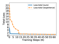
(a) $Loss_{total}$: 2-bit

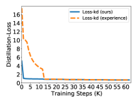
(b) $Loss_{kd}$: 2-bit

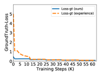
(c) $Loss_{gt}$ 2-bit

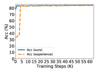
(d) $Accuracy$: 2-bit

Figure 3: The impact on total training loss, distillation loss, ground truth loss and accuracy when implementing our proposed KDLSQ-BERT by using different scale-factor initialization. The quantization bit ”W-E-A (#bit)” is set to 2-2-8. The experimental results are tested by adopting ”mnli” and ”TinyBERT”.

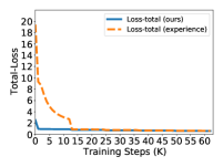
(a) $Loss_{total}$: 4-bit

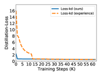
(b) $Loss_{kd}$: 4-bit

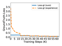
(c) $Loss_{gt}$: 4-bit

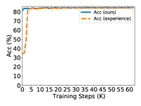
(d) $Accuracy$: 4-bit

Figure 4: The impact on total training loss, distillation loss, ground truth loss and accuracy when implementing our proposed KDLSQ-BERT by using different scale-factor initialization. The quantization bit ”W-E-A (#bit)” is set to 4-4-8. The experimental results are tested by adopting ”mnli” and ”TinyBERT”.

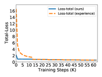
(a) $Loss_{total}$: 6-bit

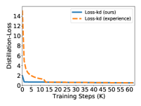
(b) $Loss_{kd}$: 6-bit

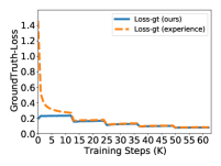
(c) $Loss_{gt}$: 6-bit

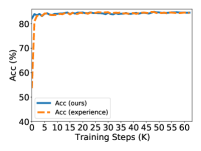
(d) $Accuracy$: 6-bit

Figure 5: The impact on total training loss, distillation loss, ground truth loss and accuracy when implementing our proposed KDLSQ-BERT by using different scale-factor initialization.The quantization bit ”W-E-A (#bit)” is set to 6-6-8. The experimental results are tested by adopting ”mnli” and ”TinyBERT”.

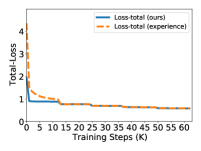
(a) $Loss_{total}$: 8-bit

(b) $Loss_{kd}$: 8-bit

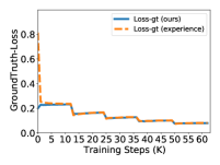
(c) $Loss_{gt}$: 8-bit

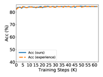
(d) $Accuracy$: 8-bit

Figure 6: The impact on total training loss, distillation loss, ground truth loss and accuracy when implementing our proposed KDLSQ-BERT by using different scale-factor initialization. The quantization bit ”W-E-A (#bit)” is set to 8-8-8. The experimental results are tested by adopting ”mnli” and ”TinyBERT”.

From Figure 3 $\sim$ Figure 6, it illustrates the experimental results related to ”mnli”. As can be seen that compared with the experience value for scale-factor initialization, the correlated training loss and model accuracy have faster convergence speed when applying Algorithm 1 to do scale-factor initialization. The main reason is that Algorithm 1 can provide well initialized scale-factors for quantization training, such that a tensor that needs to be quantized can be retained main information after the truncation. Also, note that the results from the figures show other two important information. One is that all initialized training losses (that’s, the initialized $Loss_{total}$, $Loss_{kd}$ and $Loss_{gt}$) decrease as the weight quantization bit increases. It implies that bigger quantization bit is good to accelerate the training convergence. The other one is that all correlated training losses can be reduced effectively through the training process, which further reveals that combining $Loss_{kd}$ with $Loss_{gt}$ for training is good to improve the model accuracy performance.

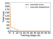
(a) $Loss_{total}$: 2-bit

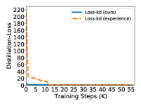
(b) $Loss_{kd}$: 2-bit

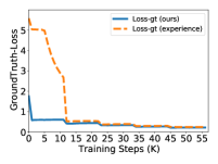
(c) $Loss_{gt}$: 2-bit

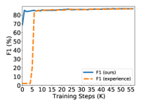
(d) $F1$: 2-bit

Figure 7: The impact on total training loss, distillation loss, ground truth loss and accuracy when implementing our proposed KDLSQ-BERT by using different scale-factor initialization. The quantization bit ”W-E-A (#bit)” is set to 2-2-8. The experimental results are tested by adopting ”SQuAD 1.1” and ”TinyBERT”.

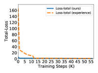
(a) $Loss_{total}$: 4-bit

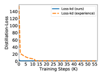
(b) $Loss_{kd}$: 4-bit

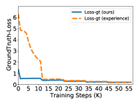
(c) $Loss_{gt}$: 4-bit

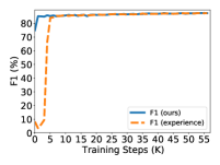
(d) $F1$: 4-bit

Figure 8: The impact on total training loss, distillation loss, ground truth loss and accuracy when implementing our proposed KDLSQ-BERT by using different scale-factor initialization. The quantization bit ”W-E-A (#bit)” is set to 4-4-8. The experimental results are tested by adopting ”SQuAD 1.1” and ”TinyBERT”

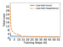
(a) $Loss_{total}$: 6-bit

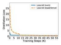
(b) $Loss_{kd}$: 6-bit

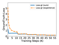
(c) $Loss_{gt}$: 6-bit

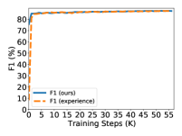
(d) $F1$: 6-bit

Figure 9: The impact on total training loss, distillation loss, ground truth loss and accuracy when implementing our proposed KDLSQ-BERT by using different scale-factor initialization. The quantization bit ”W-E-A (#bit)” is set to 6-6-8. The experimental results are tested by adopting ”SQuAD 1.1” and ”TinyBERT”

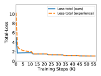
(a) $Loss_{total}$: 8-bit

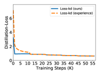
(b) $Loss_{kd}$: 8-bit

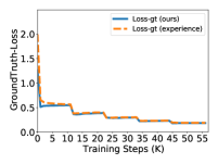
(c) $Loss_{gt}$: 8-bit

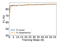
(d) $F1$: 8-bit

Figure 10: The impact on total training loss, distillation loss, ground truth loss and accuracy when implementing our proposed KDLSQ-BERT by using different scale-factor initialization. The quantization bit ”W-E-A (#bit)” is set to 8-8-8. The experimental results are tested by adopting ”SQuAD 1.1” and ”TinyBERT”

For the ”SQuAD 1.1” related to the question-answering task, Figure 7 $\sim$ Figure 10 demonstrate the same results as those of ”mnli”. As illustrated in those figures, when using Algorithm 1 to do initialization for scale-factors, the correlated training losses and model accuracy can get faster convergence speed as the training step goes. This is because the scale-factors can be well initialized by using our scale-factor initialization method, such that an effective truncation for the quantized tensor results in good training convergence. Besides, all correlated training losses can be converged effectively, which proves that it is a good way to enhance the model accuracy by setting both $Loss_{kd}$ and $Loss_{gt}$ as reference for model training.

4.3 Ablation Studies

According to the steps from Algorithm 2, our proposed KDLSQ-BERT mainly consists of three components including LSQ, knowledge distillation, as well as the ground truth loss based on training data set. To further analyze the effects of different components, we perform ablation study on different NLP tasks, and the specific comparison results are listed in Table 4 and Table 5. In these tables, ”LSQ+KD+Lgt” denotes our proposed KDLSQ-BERT, ”LSQ+KD” indicates LSQ along with knowledge distillation, ”LSQ” indicates LSQ method only.

Table 4: Ablation Study on GLUE benchmark.

		W-E-A	Size	MNLI	CoLA	MRPC	QNLI	QQP	RTE	SST-2	STS-B	$Average$
		(#bits)	(MB)
Full-precision	BERT-base	32-32-32	418 ($\times 1.0$)	84.463	58.081	90.625	91.964	87.762	71.119	93.119	89.823	83.369
2-bit	LSQ	2-2-8	28 ($\times 14.9$)	83.271	49.981	90.117	90.024	87.445	70.397	91.399	87.609	81.280
	LSQ+KD	2-2-8	28 ($\times 14.9$)	84.361	48.724	90.444	91.415	87.696	67.148	92.202	88.117	81.263
	LSQ+KD+Lgt	2-2-8	28 ($\times 14.9$)	84.564	49.418	90.290	91.452	88.071	67.509	92.775	88.117	81.524
4-bit	LSQ	4-4-8	54 ($\times 7.7$)	84.218	57.738	90.183	91.305	87.827	72.924	93.005	89.569	83.359
	LSQ+KD	4-4-8	54 ($\times 7.7$)	85.064	59.274	90.694	92.239	88.027	72.924	93.693	89.697	83.951
	LSQ+KD+Lgt	4-4-8	54 ($\times 7.7$)	85.329	60.646	91.394	92.165	88.503	72.729	93.349	89.697	84.221
6-bit	LSQ	6-6-8	80 ($\times 5.2$)	84.463	60.749	85.583	91.781	88.042	74.368	93.119	89.495	83.950
	LSQ+KD	6-6-8	80 ($\times 5.2$)	85.257	59.426	91.312	92.165	87.987	71.841	93.463	90.000	83.931
	LSQ+KD+Lgt	6-6-8	80 ($\times 5.2$)	85.329	61.482	91.003	92.367	88.463	71.480	93.807	90.000	84.241
8-bit	LSQ	8-8-8	106 ($\times 3.9$)	84.401	59.937	90.941	91.122	87.832	72.202	93.349	89.569	83.669
	LSQ+KD	8-8-8	106 ($\times 3.9$)	85.084	59.994	91.096	92.165	87.947	71.841	93.807	89.944	83.985
	LSQ+KD+Lgt	8-8-8	106 ($\times 3.9$)	85.308	60.774	91.826	92.147	88.439	71.841	93.693	89.944	84.247
Full-precision	TinyBERT	32-32-32	258 ($\times 1.6$)	84.768	54.175	91.319	90.793	87.966	71.841	90.252	89.792	82.613
2-bit	LSQ	2-2-8	18 ($\times 23.2$)	83.179	49.344	90.501	88.285	87.635	63.899	91.514	87.704	80.257
	LSQ+KD	2-2-8	18 ($\times 23.2$)	83.953	49.498	90.690	90.170	87.642	62.455	92.661	87.539	80.576
	LSQ+KD+Lgt	2-2-8	18 ($\times 23.2$)	83.902	49.047	91.100	90.518	88.038	64.260	92.661	87.539	80.883
4-bit	LSQ	4-4-8	34 ($\times 12.3$)	84.340	52.588	89.949	90.170	87.944	74.368	92.431	89.767	82.695
	LSQ+KD	4-4-8	34 ($\times 12.3$)	84.727	54.062	91.161	91.269	87.984	71.119	92.775	89.825	82.865
	LSQ+KD+Lgt	4-4-8	34 ($\times 12.3$)	84.962	54.415	91.192	91.671	88.300	72.202	92.890	89.825	83.182
6-bit	LSQ	6-6-8	50 ($\times 8.3$)	84.432	53.321	89.865	90.591	88.030	76.173	92.202	88.041	82.832
	LSQ+KD	6-6-8	50 ($\times 8.3$)	84.819	54.302	91.478	91.177	88.007	71.841	93.006	89.895	83.066
	LSQ+KD+Lgt	6-6-8	50 ($\times 8.3$)	85.013	54.293	91.035	91.580	88.333	73.285	93.006	89.895	83.305
8-bit	LSQ	8-8-8	65 ($\times 6.4$)	84.615	53.807	90.508	90.957	88.092	76.173	92.288	89.950	83.299
	LSQ+KD	8-8-8	65 ($\times 6.4$)	84.911	54.521	91.319	91.140	88.039	72.563	92.775	89.958	83.153
	LSQ+KD+Lgt	8-8-8	65 ($\times 6.4$)	85.013	54.793	91.130	91.580	88.315	73.646	92.890	89.958	83.416

Table 5: Ablation Study on SQuAD.

		W-E-A	Size	SQuAD 1.1	SQuAD 2.0	$Average$
		(#bits)	(MB)
Full-precision	BERT-base	32-32-32	418 ($\times 1.0$)	88.696	77.725	83.210
2-bit	LSQ	2-2-8	28 ($\times 14.9$)	84.105	74.254	79.179
	LSQ+KD	2-2-8	28 ($\times 14.9$)	88.794	77.619	83.207
	LSQ+KD+Lgt	2-2-8	28 ($\times 14.9$)	88.447	78.400	83.423
4-bit	LSQ	4-4-8	54 ($\times 7.7$)	86.098	76.840	81.469
	LSQ+KD	4-4-8	54 ($\times 7.7$)	89.236	78.421	83.828
	LSQ+KD+Lgt	4-4-8	54 ($\times 7.7$)	89.207	78.965	84.086
6-bit	LSQ	6-6-8	80 ($\times 5.2$)	86.357	76.438	81.398
	LSQ+KD	6-6-8	80 ($\times 5.2$)	89.296	78.412	83.854
	LSQ+KD+Lgt	6-6-8	80 ($\times 5.2$)	89.280	78.905	84.092
8-bit	LSQ	8-8-8	106 ($\times 3.9$)	86.576	76.334	81.455
	LSQ+KD	8-8-8	106 ($\times 3.9$)	89.292	78.500	83.896
	LSQ+KD+Lgt	8-8-8	106 ($\times 3.9$)	89.218	79.330	84.274
Full-precision	TinyBERT	32-32-32	258 ($\times 1.6$)	87.527	77.730	82.629
2-bit	LSQ	2-2-8	18 ($\times 23.2$)	84.769	73.518	79.144
	LSQ+KD	2-2-8	18 ($\times 23.2$)	86.053	76.747	81.400
	LSQ+KD+Lgt	2-2-8	18 ($\times 23.2$)	86.635	76.889	81.762
4-bit	LSQ	4-4-8	34 ($\times 12.3$)	85.667	75.304	80.486
	LSQ+KD	4-4-8	34 ($\times 12.3$)	87.495	77.967	82.731
	LSQ+KD+Lgt	4-4-8	34 ($\times 12.3$)	87.887	77.981	82.934
6-bit	LSQ	6-6-8	50 ($\times 8.3$)	85.902	75.640	80.771
	LSQ+KD	6-6-8	50 ($\times 8.3$)	87.581	78.067	82.824
	LSQ+KD+Lgt	6-6-8	50 ($\times 8.3$)	87.944	78.279	83.111
8-bit	LSQ	8-8-8	65 ($\times 6.4$)	86.587	75.908	81.247
	LSQ+KD	8-8-8	65 ($\times 6.4$)	87.587	78.079	82.833
	LSQ+KD+Lgt	8-8-8	65 ($\times 6.4$)	87.948	78.302	83.125

From the tables, it demonstrates that for both the GLUE benchmark and the SQuAD, ”LSQ+KD+Lgt” can perform better accuracy than both ”LSQ” and ”LSQ+KD” on average. This is because the training loss for ”LSQ+KD+Lgt” involves more reference information to improve the training result. The correlated information mainly include knowledge from both the teacher model and the ground truth labels of the training data. Different from ”LSQ+KD+Lgt”, ”LSQ” involves only knowledge from the ground truth labels of the training data, and ”LSQ+KD” involves only the knowledge of the teacher model. Note that the experimental results show that for the GLUE benchmark, ”LSQ” and ”LSQ+KD” can obtain almost the same accuracy in the same bit quantization; while for the SQuAD, ”LSQ+KD” can perform about 2.0% higher accuracy than ”LSQ” when doing the same bit quantization. As a result, it is hard to determine if ”LSQ+KD” is better than ”LSQ” or not because both methods apply different knowledge for quantization training. However, the results from the tables prove that KDLSQ-BERT (e.g., ”LSQ+KD+Lgt”) performs better not only in high-bit (e.g., 8-bit) quantization, but also in low-bit (e.g., 2-bit) quantization. Consequently, KDLSQ-BERT is an effective and practical training method for BERT quantization.

4.4 Experimental Analysis on Low Bit Quantization

To further study the performance of our method on different NLP tasks, we conduct KDLSQ-BERT by setting KDLSQ-BERT in ultra-low bit quantization. The specific experimental results are presented in Table 6 and Table 7, respectively. As shown in the tables, it demonstrates that for both the GLUE benchmark and the SQuAD, our quantization method can obtain the same accuracy as the full-precision base-line model even if doing the ultra-low bit quantization. Especially, it should be noted that compared with the quantization configuration of ”4-4-2” and ”2-2-2”, setting ”2-2-4” can get almost the same accuracy performance as the full-precision base-line model. On the one hand, it proves that activation quantization is more sensitive to affect the accuracy performance than the weight quantization. On the other hand, these empirical results tell us that it 2-bit is enough for weight quantization when using our method to do quantization training. Therefore, even if conducting ultra-low bit quantization, our method not only can guarantee the accuracy performance, but also can get an impressive compression ratio.

Table 6: Low bit quantization of KDLSQ-BERT on the GLUE benchmark.

		W-E-A	Size	MNLI	CoLA	MRPC	QNLI	QQP	RTE	SST-2	STS-B	$Average$
		(#bit)	(MB)
Full-precision	BERT-base	32-32-32	418 ($\times 1.0$)	84.463	58.081	90.625	91.964	87.762	71.119	93.119	89.823	83.369
2-bit	KDLSQ-BERT (ours)	2-2-2	28 ($\times 14.9$)	83.607	54.885	90.000	90.536	87.962	66.065	92.775	85.854	81.460
2-bit	KDLSQ-BERT (ours)	2-2-4	28 ($\times 14.9$)	85.013	58.081	91.388	92.092	87.996	73.646	93.693	89.989	83.987
4-bit	KDLSQ-BERT (ours)	4-4-2	54 ($\times 7.7$)	83.535	54.844	89.619	90.902	88.085	67.870	93.005	87.095	81.869
4-bit	KDLSQ-BERT (ours)	4-4-4	54 ($\times 7.7$)	85.115	60.132	92.063	92.257	88.355	73.285	93.234	89.851	84.287
4-bit	KDLSQ-BERT (ours)	4-4-6	54 ($\times 7.7$)	85.094	61.788	92.171	92.367	88.526	71.480	93.693	90.197	84.414
4-bit	KDLSQ-BERT (ours)	4-4-8	54 ($\times 7.7$)	84.218	57.738	90.183	91.305	87.827	72.924	93.005	89.569	83.359
Full-precision	TinyBERT	32-32-32	258 ($\times 1.6$)	84.768	54.175	91.319	90.793	87.966	71.841	90.252	89.792	82.613
2-bit	KDLSQ-BERT (ours)	2-2-2	18 ($\times 23.2$)	82.354	45.805	89.003	89.694	87.721	65.343	92.431	84.460	79.602
2-bit	KDLSQ-BERT (ours)	2-2-4	18 ($\times 23.2$)	84.483	54.944	90.909	91.177	88.376	75.451	93.119	89.420	83.485
4-bit	KDLSQ-BERT (ours)	4-4-2	34 ($\times 12.3$)	82.517	47.306	89.608	89.658	88.005	65.704	92.202	85.430	80.054
4-bit	KDLSQ-BERT (ours)	4-4-4	34 ($\times 12.3$)	84.697	55.130	90.630	91.580	88.414	74.007	93.119	89.580	83.395
4-bit	KDLSQ-BERT (ours)	4-4-6	34 ($\times 12.3$)	84.768	55.727	91.388	91.781	88.394	75.812	93.234	89.952	83.882
4-bit	KDLSQ-BERT (ours)	4-4-8	34 ($\times 12.3$)	84.962	54.415	91.192	91.671	88.300	72.202	92.890	89.825	83.182

Table 7: Low bit quantization of KDLSQ-BERT on the SQuAD.

		W-E-A	Size	SQuAD 1.1	SQuAD 2.0	$Average$
		(#bit)	(MB)
Full-precision	BERT-base	32-32-32	418 ($\times 1.0$)	88.696	77.725	83.210
2-bit	KDLSQ-BERT (ours)	2-2-2	28 ($\times 14.9$)	84.818	73.339	79.078
2-bit	KDLSQ-BERT (ours)	2-2-4	28 ($\times 14.9$)	88.996	78.213	83.604
4-bit	KDLSQ-BERT (ours)	4-4-2	54 ($\times 7.7$)	85.070	77.725	81.397
4-bit	KDLSQ-BERT (ours)	4-4-4	54 ($\times 7.7$)	88.998	77.919	83.458
4-bit	KDLSQ-BERT (ours)	4-4-6	54 ($\times 7.7$)	89.070	78.342	83.706
4-bit	KDLSQ-BERT (ours)	4-4-8	54 ($\times 7.7$)	89.207	78.965	84.086
Full-precision	TinyBERT	32-32-32	258 ($\times 1.6$)	87.527	77.730	82.629
2-bit	KDLSQ-BERT (ours)	2-2-2	18 ($\times 23.2$)	80.695	70.124	75.410
2-bit	KDLSQ-BERT (ours)	2-2-4	18 ($\times 23.2$)	86.858	77.197	82.027
4-bit	KDLSQ-BERT (ours)	4-4-2	34 ($\times 12.3$)	81.099	70.794	75.946
4-bit	KDLSQ-BERT (ours)	4-4-4	34 ($\times 12.3$)	86.902	77.400	82.151
4-bit	KDLSQ-BERT (ours)	4-4-6	34 ($\times 12.3$)	87.569	77.796	82.682
4-bit	KDLSQ-BERT (ours)	4-4-8	34 ($\times 12.3$)	87.887	77.981	82.934

5 Conclusion and Future Work

In this work, we proposed a novel quantization method KDLSQ-BERT to quantize the Transformer-based models such as BERT. In addition to exploiting the ground truth for training loss calculation, the main feature of KDLSQ-BERT is that the KD technique is leveraged to transfer the knowledge from a ”teacher” BERT to a ”student” BERT when doing LSQ to quantize that ”student” BERT. Empirical experiments show that KDLSQ-BERT not only can outperform the state-of-the-art BERT quantization methods, but also can achieve high accuracy when doing ultra low-bit (e.g., 2-bit) weight quantization, and even can perform comparable performance as the full-precision base-line model. In the near future we will explore how to quantize other NLP models in low-bit (such as 2-bit) on the basis of LSQ.

References

- Bengio et al. (2013) Yoshua Bengio, Nicholas Léonard, and Aaron Courville. Estimating or propagating gradients through stochastic neurons for conditional computation. arXiv preprint arXiv:1308.3432, 2013.
- Chicco & Jurman (2020) Davide Chicco and Giuseppe Jurman. The advantages of the matthews correlation coefficient (mcc) over f1 score and accuracy in binary classification evaluation. BMC genomics, 21(1):6, 2020.
- Clark et al. (2019) Kevin Clark, Urvashi Khandelwal, Omer Levy, and Christopher D Manning. What does bert look at? an analysis of bert’s attention. arXiv preprint arXiv:1906.04341, 2019.
- Dehghani et al. (2018) Mostafa Dehghani, Stephan Gouws, Oriol Vinyals, Jakob Uszkoreit, and Łukasz Kaiser. Universal transformers. arXiv preprint arXiv:1807.03819, 2018.
- Derczynski (2016) Leon Derczynski. Complementarity, f-score, and nlp evaluation. In Proceedings of the Tenth International Conference on Language Resources and Evaluation (LREC’16), pp. 261–266, 2016.
- Devlin et al. (2018) Jacob Devlin, Ming-Wei Chang, Kenton Lee, and Kristina Toutanova. Bert: Pre-training of deep bidirectional transformers for language understanding. arXiv preprint arXiv:1810.04805, 2018.
- Esser et al. (2019) Steven K Esser, Jeffrey L McKinstry, Deepika Bablani, Rathinakumar Appuswamy, and Dharmendra S Modha. Learned step size quantization. arXiv preprint arXiv:1902.08153, 2019.
- Fan et al. (2019) Angela Fan, Edouard Grave, and Armand Joulin. Reducing transformer depth on demand with structured dropout. arXiv preprint arXiv:1909.11556, 2019.
- Fan et al. (2020) Angela Fan, Pierre Stock, Benjamin Graham, Edouard Grave, Rémi Gribonval, Hervé Jégou, and Armand Joulin. Training with quantization noise for extreme model compression. 2020.
- Hinton et al. (2015) Geoffrey Hinton, Oriol Vinyals, and Jeff Dean. Distilling the knowledge in a neural network. arXiv preprint arXiv:1503.02531, 2015.
- Hou et al. (2020) Lu Hou, Lifeng Shang, Xin Jiang, and Qun Liu. Dynabert: Dynamic bert with adaptive width and depth. arXiv preprint arXiv:2004.04037, 2020.
- Hu et al. (2018) Minghao Hu, Yuxing Peng, Furu Wei, Zhen Huang, Dongsheng Li, Nan Yang, and Ming Zhou. Attention-guided answer distillation for machine reading comprehension. arXiv preprint arXiv:1808.07644, 2018.
- Jacob et al. (2018) Benoit Jacob, Skirmantas Kligys, Bo Chen, Menglong Zhu, Matthew Tang, Andrew Howard, Hartwig Adam, and Dmitry Kalenichenko. Quantization and training of neural networks for efficient integer-arithmetic-only inference. In Proceedings of the IEEE Conference on Computer Vision and Pattern Recognition, pp. 2704–2713, 2018.
- Jain et al. (2019) Sambhav R Jain, Albert Gural, Michael Wu, and Chris H Dick. Trained quantization thresholds for accurate and efficient fixed-point inference of deep neural networks. arXiv preprint arXiv:1903.08066, 2019.
- Jiao et al. (2019) Xiaoqi Jiao, Yichun Yin, Lifeng Shang, Xin Jiang, Xiao Chen, Linlin Li, Fang Wang, and Qun Liu. Tinybert: Distilling bert for natural language understanding. arXiv preprint arXiv:1909.10351, 2019.
- Kim et al. (2019) Jangho Kim, Yash Bhalgat, Jinwon Lee, Chirag Patel, and Nojun Kwak. Qkd: Quantization-aware knowledge distillation. arXiv preprint arXiv:1911.12491, 2019.
- Kim & Rush (2016) Yoon Kim and Alexander M Rush. Sequence-level knowledge distillation. arXiv preprint arXiv:1606.07947, 2016.
- Krishnamoorthi (2018) Raghuraman Krishnamoorthi. Quantizing deep convolutional networks for efficient inference: A whitepaper. arXiv preprint arXiv:1806.08342, 2018.
- Lan et al. (2019) Zhenzhong Lan, Mingda Chen, Sebastian Goodman, Kevin Gimpel, Piyush Sharma, and Radu Soricut. Albert: A lite bert for self-supervised learning of language representations. arXiv preprint arXiv:1909.11942, 2019.
- Liu et al. (2019) Yinhan Liu, Myle Ott, Naman Goyal, Jingfei Du, Mandar Joshi, Danqi Chen, Omer Levy, Mike Lewis, Luke Zettlemoyer, and Veselin Stoyanov. Roberta: A robustly optimized bert pretraining approach. arXiv preprint arXiv:1907.11692, 2019.
- Ma et al. (2019) Xindian Ma, Peng Zhang, Shuai Zhang, Nan Duan, Yuexian Hou, Ming Zhou, and Dawei Song. A tensorized transformer for language modeling. In Advances in Neural Information Processing Systems, pp. 2232–2242, 2019.
- Mao et al. (2020) Yihuan Mao, Yujing Wang, Chufan Wu, Chen Zhang, Yang Wang, Yaming Yang, Quanlu Zhang, Yunhai Tong, and Jing Bai. Ladabert: Lightweight adaptation of bert through hybrid model compression. arXiv preprint arXiv:2004.04124, 2020.
- McCarley (2019) J Scott McCarley. Pruning a bert-based question answering model. arXiv preprint arXiv:1910.06360, 2019.
- Michel et al. (2019) Paul Michel, Omer Levy, and Graham Neubig. Are sixteen heads really better than one? In Advances in Neural Information Processing Systems, pp. 14014–14024, 2019.
- Polino et al. (2018) Antonio Polino, Razvan Pascanu, and Dan Alistarh. Model compression via distillation and quantization. arXiv preprint arXiv:1802.05668, 2018.
- Prato et al. (2019) Gabriele Prato, Ella Charlaix, and Mehdi Rezagholizadeh. Fully quantized transformer for improved translation. arXiv preprint arXiv:1910.10485, 2019.
- Rajpurkar et al. (2016) Pranav Rajpurkar, Jian Zhang, Konstantin Lopyrev, and Percy Liang. Squad: 100,000+ questions for machine comprehension of text. arXiv preprint arXiv:1606.05250, 2016.
- Romero et al. (2014) Adriana Romero, Nicolas Ballas, Samira Ebrahimi Kahou, Antoine Chassang, Carlo Gatta, and Yoshua Bengio. Fitnets: Hints for thin deep nets. arXiv preprint arXiv:1412.6550, 2014.
- Sanh et al. (2019) Victor Sanh, Lysandre Debut, Julien Chaumond, and Thomas Wolf. Distilbert, a distilled version of bert: smaller, faster, cheaper and lighter. arXiv preprint arXiv:1910.01108, 2019.
- Shen et al. (2020) Sheng Shen, Zhen Dong, Jiayu Ye, Linjian Ma, Zhewei Yao, Amir Gholami, Michael W Mahoney, and Kurt Keutzer. Q-bert: Hessian based ultra low precision quantization of bert. In AAAI, pp. 8815–8821, 2020.
- Stock et al. (2019) Pierre Stock, Armand Joulin, Rémi Gribonval, Benjamin Graham, and Hervé Jégou. And the bit goes down: Revisiting the quantization of neural networks. arXiv preprint arXiv:1907.05686, 2019.
- Sun et al. (2019) Siqi Sun, Yu Cheng, Zhe Gan, and Jingjing Liu. Patient knowledge distillation for bert model compression. arXiv preprint arXiv:1908.09355, 2019.
- Vaswani et al. (2017) Ashish Vaswani, Noam Shazeer, Niki Parmar, Jakob Uszkoreit, Llion Jones, Aidan N Gomez, Ł ukasz Kaiser, and Illia Polosukhin. Attention is all you need. In I. Guyon, U. V. Luxburg, S. Bengio, H. Wallach, R. Fergus, S. Vishwanathan, and R. Garnett (eds.), Advances in Neural Information Processing Systems 30, pp. 5998–6008. Curran Associates, Inc., 2017. URL http://papers.nips.cc/paper/7181-attention-is-all-you-need.pdf.
- Voita et al. (2019) Elena Voita, David Talbot, Fedor Moiseev, Rico Sennrich, and Ivan Titov. Analyzing multi-head self-attention: Specialized heads do the heavy lifting, the rest can be pruned. arXiv preprint arXiv:1905.09418, 2019.
- Wang et al. (2018) Alex Wang, Amanpreet Singh, Julian Michael, Felix Hill, Omer Levy, and Samuel R Bowman. Glue: A multi-task benchmark and analysis platform for natural language understanding. arXiv preprint arXiv:1804.07461, 2018.
- Wang et al. (2020) Wenhui Wang, Furu Wei, Li Dong, Hangbo Bao, Nan Yang, and Ming Zhou. Minilm: Deep self-attention distillation for task-agnostic compression of pre-trained transformers. arXiv preprint arXiv:2002.10957, 2020.
- Yang et al. (2019) Zhilin Yang, Zihang Dai, Yiming Yang, Jaime Carbonell, Russ R Salakhutdinov, and Quoc V Le. Xlnet: Generalized autoregressive pretraining for language understanding. In Advances in neural information processing systems, pp. 5753–5763, 2019.
- Zadeh & Moshovos (2020) Ali Hadi Zadeh and Andreas Moshovos. Gobo: Quantizing attention-based nlp models for low latency and energy efficient inference. arXiv preprint arXiv:2005.03842, 2020.
- Zafrir et al. (2019) Ofir Zafrir, Guy Boudoukh, Peter Izsak, and Moshe Wasserblat. Q8bert: Quantized 8bit bert. arXiv preprint arXiv:1910.06188, 2019.
- Zhang et al. (2020) Wei Zhang, Lu Hou, Yichun Yin, Lifeng Shang, Xiao Chen, Xin Jiang, and Qun Liu. Ternarybert: Distillation-aware ultra-low bit bert. arXiv preprint arXiv:2009.12812, 2020.