Erratum:”Quasi-objective coherent structure diagnostics
from single trajectories” [Chaos 31, 043131 (2021)]

This erratum corrects a mistake in our previously published paper [1]. Theorem 3 is incorrect as stated because the extended Euclidean frame changes of the form (32) are nonlinear transformations of the extended phases space. Their Jacobians generally does not preserve lengths and angles, and hence the scalar fields $\mathrm{TSE}$, $\overline{\mathrm{TSE}}$ and $\mathrm{\overline{\mathrm{TRA}}}$ are not invariant under these transformations.

Theorem 3 can be corrected by modifying assumption (A1) for unsteady flows as

(A3)                                                $\left|\partial_{t}\mathbf{v}(\mathbf{x}(t),t)\right|\ll\left|\mathbf{a}(t)\right|$,

where $\mathbf{a}(t):=\ddot{\mathbf{x}}(t)$ denoted the Lagrangian acceleration. This reflects the assumption that Lagrangian time scales dominate Eulerian time scales in geophysical flows, which originally motivated our study. On specific flow domains, (A3) can be a priori verified from characteristic velocity-, length- and time-scales (see, e.g, Ref. [2], p. 88). Assumption (A3) also eliminates the need to use the extended phase space in our arguments and enables us to set $\mathrm{v}_{0}=0$ in our formulas. Figure 1. shows that (A3) is satisfied on average for both the AVISO data set and the unsteady ABC flow example we considered in [1].

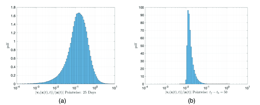
Figure 1: Verification of assumption (A3) for our two examples in [1]: Probability density function (pdf) of the values of $\left|\partial_{t}\mathbf{v}(\mathbf{x}(t),t)\right|/\left|\mathbf{a}(t)\right|$ for assumption (A3) in (a) the AVISO data set example (b) the unsteady ABC flow example. The pdf is measured in probability per unit increment.

The evolution of the Lagrangian velocity $\boldsymbol{v}(t):=\mathbf{v}(\mathbf{x}(t),t)$ is nearly material in frames satisfying (A3). Additionally, such frames must be related to each other via Euclidean coordinate transformations $\mathbf{x}=\mathbf{Q}(t)\mathbf{y}+\mathbf{b}(t)$ with $\left|\dot{\mathbf{Q}}\right|,\left|\dot{\mathbf{b}}\right|,\left|\ddot{\mathbf{Q}}\right|,\left|\ddot{\mathbf{b}}\right|\ll 1$, i.e., via slowly varying (geophysical) frame changes, in order for the $\mathrm{TSE}$, $\overline{\mathrm{TSE}}$ and $\mathrm{\overline{\mathrm{TRA}}}$ to return approximately the same values in the new frames. More specifically, our revised definition of quasi-objectivity for a scalar field is that it has to approximate the same objective quantity in all frames related to each other by slowly varying Euclidean transformation.

In any frame satisfying (A3), therefore, the single-trajectory diagnostics $\lambda{}_{t_{0}}^{t_{N}}(\mathbf{\boldsymbol{x}}_{0},\boldsymbol{v}(t_{0}))$ and $\bar{\lambda}{}_{t_{0}}^{t_{N}}(\mathbf{\boldsymbol{x}}_{0},\boldsymbol{v}(t_{0}))$ will closely approximate the corresponding objective measures (averaged stretching exponent and averaged hyperbolicity strength) of material elements initially aligned with $\boldsymbol{v}(t_{0})$. This implies the quasi-objectivity of these single-trajectory diagnostics by the above revision of the definition of Ref. [1]. A similar statement holds for the rotation diagnostic $\bar{\alpha}_{t_{0}}^{t_{N}}(\mathbf{\boldsymbol{x}}_{0},\boldsymbol{v}(t_{0}))$ under assumptions (A2)-(A3). In summary, the corrected Theorem 3 reads as follows:

Theorem 3.

(i) Under assumption (A3), the trajectory stretching exponents (TSEs), defined as

$$\mathrm{TSE}_{t_{0}}^{t_{N}}(\boldsymbol{x}\mathbf{}_{0})=\frac{1}{t_{N}-t_{0}}\log\frac{\left|\dot{\mathbf{x}}(t_{N})\right|}{\left|\dot{\mathbf{x}}(t_{0})\right|},\qquad\overline{\mathrm{TSE}}_{t_{0}}^{t_{N}}(\boldsymbol{x}\mathbf{}_{0})=\frac{1}{t_{N}-t_{0}}\sum_{i=0}^{N-1}\left|\log\frac{\left|\dot{\mathbf{x}}(t_{i+1})\right|}{\left|\dot{\mathbf{x}}(t_{i})\right|}\right|,$$

are quasi-objective measures of trajectory stretching and hyperbolicity strength.

(ii) Under assumptions (A2)-(A3), the trajectory angular velocity ($\mathrm{\overline{\mathrm{TRA}}}$), defined as

$$\mathrm{\overline{\mathrm{TRA}}}_{t_{0}}^{t_{N}}(\boldsymbol{x}\mathbf{}_{0}) =\frac{1}{t_{N}-t_{0}}\sum_{i=0}^{N-1}\cos^{-1}\frac{\left\langle\dot{\mathbf{\boldsymbol{x}}}(t_{i}),\dot{\mathbf{\boldsymbol{x}}}(t_{i+1})\right\rangle}{\left|\dot{\mathbf{\boldsymbol{x}}}(t_{i})\right|\left|\dot{\mathbf{\boldsymbol{x}}}(t_{i+1})\right|},$$

is a quasi-objective measure of total trajectory rotation.

Figures 2-5 below are revised version of Figs. 1,2,4 and 5 of Ref. [1], showing that our main conclusions remain valid under the corrected implementation of Theorem 3. Figures 6 and 7 need no revision, because their computations were carried out on an objective vector field for which assumptions (A2) and (A3) are not required.

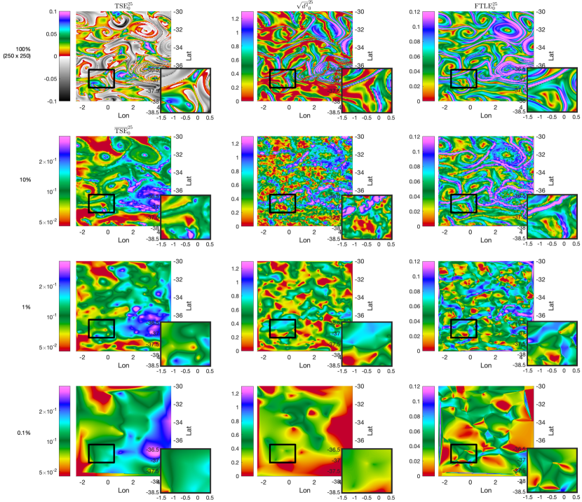
Figure 2: Stretching metric comparisons for AVISO ocean surface current fields. The top row shows computations at full resolution with the lower rows having progressively reduced resolution by randomly subsampling with fewer trajectories.

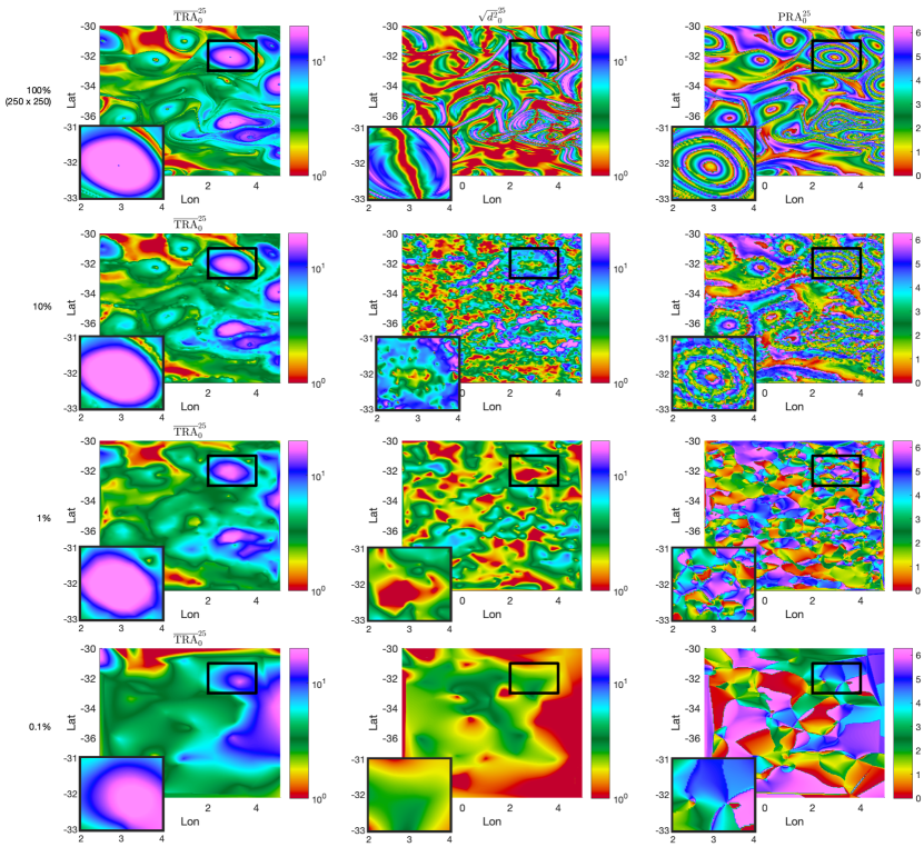
Figure 3: Rotation metric comparisons for AVISO ocean surface current fields. The top row shows computations at full resolution with the lower rows having progressively reduced resolution by randomly subsampling with fewer trajectories. We display $\sqrt{d^{2}}$ here for clarity.

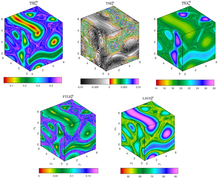
Figure 4: Elliptic and hyperbolic LCSs in the unsteady ABC flow (41). The plots compare quasi-objective, single-trajectory metrics ($\mathrm{TSE_{0}^{50}(\boldsymbol{x}\mathbf{}_{0})}$ and $\mathrm{\mathrm{\overline{\mathrm{TRA}}{}_{0}^{50}}}(\boldsymbol{x}\mathbf{}_{0})$) with objective LCS metrics ($\mathrm{FTLE}_{0}^{50}(\boldsymbol{x}\mathbf{}_{0})$ and $\mathrm{LAVD}_{0}^{50}(\boldsymbol{x}\mathbf{}_{0})$) that require multiple neighboring trajectories or detailed knowledge of the velocity field.

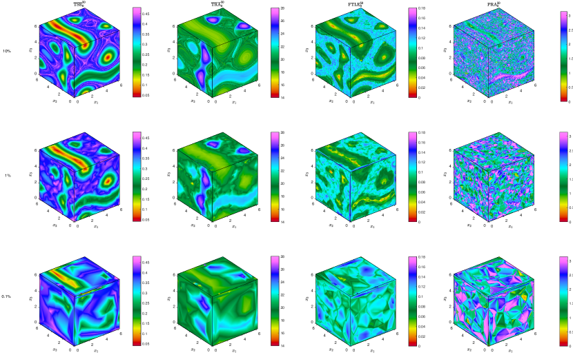
Figure 5: Elliptic and hyperbolic LCS in the randomly subsampled unsteady ABC flow (41). The plots compare quasi-objective single-trajectory metrics ($\mathrm{\overline{TSE}{}_{0}^{50}}(\boldsymbol{x}\mathbf{}_{0})$ and $\mathrm{\overline{TRA}_{0}^{50}}(\boldsymbol{x}\mathbf{}_{0})$) with LCS metrics ($\mathrm{FTLE}_{0}^{50}(\boldsymbol{x}\mathbf{}_{0})$ and $\mathrm{PRA}_{0}^{50}(\boldsymbol{x}\mathbf{}_{0})$), whose computation requires multiple neighboring trajectories. The initial condition grid for trajectories is randomized and its density is gradually decreased to $0.1\%$ of its initial value.

We would like to thank Holger Theisel, Anke Friederici and Tobias Günther for pointing out the invalidity of our original Theorem 3 via a counterexample in [3]. We are also grateful to Bálint Kaszás for his helpful comments and for bringing Ref. [2] to our attention.

References

[1]Haller, G., Aksamit, N., and Encinas Bartos, A.P.
Quasi-objective coherent structure diagnostics from single trajectories,
Chaos31, 043131 (2021)
[2]Pedlosky, J., Geophysical Fluid Dynamics.
Springer, New York (1987).
[3]Theisel, H., Friederici, A., and Günther, T.,
Objective flow measures based on few trajectories. https://arxiv.org/abs/2202.09566
(2022).