Impact of Distributed Rate Limiting on Load Distribution
in a Latency-sensitive Messaging Service

Abstract

The cloud’s flexibility and promise of seamless auto-scaling notwithstanding, its ability to meet service level objectives (SLOs) typically calls for some form of control in resources usage. This seemingly traditional problem gives rise to new challenges in a cloud setting, and in particular a subtle yet significant trade-off involving load-distribution decisions (the distribution of workload across available cloud resources to optimize performance), and rate control (the capping of individual workloads to prevent global over-commitment). The paper investigates this trade-off through the design and implementation of a real-time messaging system motivated by IoT applications, and demonstrates a solution capable of realizing an effective compromise. The paper’s contributions are in both explicating the source of this trade-off, and in demonstrating a possible solution.

1 Background & Motivations

1.1 Background

The cloud and its many “*aaS” instantiations [29] has ushered in a new era of access to computations, and this has in turn enabled an explosion in distributed applications, in particular in the Internet-of-Things (IoT) space [18].

IoT applications commonly involve a large volume of data generated across many sources (sensors) distributed over geographically diverse locations, and that need to be processed and often acted upon in a timely manner, e.g., for actuation purpose. Consequently, they require effective data transfer and processing solutions. The combination of the cloud’s inherent computational flexibility and scalable communication platforms are what makes it an attractive platform for IoT applications [2, 3, 25]. This has led to the development of communication platforms such as Microsoft Azure Service Bus and Amazon AWS IoT. Those platforms are based on a publish/subscribe (pub/sub) paradigm, which lets a large number of senders and receivers connect without the need for a complex mesh of one-to-one connections.

Fig. 1 illustrates the typical architecture for such a system, with topics as the abstraction used to connect publishers (senders) and subscribers (receivers). Message brokers mediate between publishers and subscribers by receiving, queueing and forwarding messages for different topics. Publishers publish messages to a broker for a given topic, with subscribers subscribing to brokers to receive messages from that topic. Scalability is realized by having multiple brokers across which to distribute the workload [36, 39], both from different topics as well as for individual topics with a heavy message load, e.g., Topic $2$ in Fig. 1. This enables rapid access to additional capacity when needed.

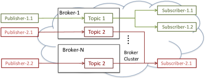
Figure 1: Pub/sub messaging platform structure

As with any shared resource, the workload of message brokers needs to be controlled to ensure that service level objectives (SLOs) are met. This is particularly important for IoT applications that require timely delivery (and processing) of their data. If an application/topic was to (accidentally or intentionally) misbehave and generate a much higher message load than anticipated, it could overwhelm the platform resources (CPU and memory), and in turn affect the SLOs of other topics. A standard approach to address this issue is to rate limit the message volume of each topic. Rate limiting is used in several public cloud platforms and commonly implemented through a software API gateway [11, 12].

In practice, the rate limiting mechanism is in the form of a token bucket [5, 38, 24, 30, 11, 51], where each message requires a token before it can be processed by its broker. In the absence of tokens, an arriving message is deemed non-conformant and waits for one (alternatively, it can be dropped). A token bucket is typically specified by two parameters, $(r,b)$, as part of the topic’s SLO. The parameter $r$ gives the rate at which tokens are generated, and therefore bounds the topic’s long-term message rate. The parameter $b$ indicates the maximum number of tokens the topic can accumulate and bounds the maximum message burst it can send without incurring an access delay (waiting for tokens). Their combination specifies the workload “envelope” [35] that the rate controller enforces.

1.2 A Motivating Example

Consider an intelligent transportation system [9] that has to process vehicle volume data acquired from tens of thousands of sensors distributed over an urban region, and respond within a second or less [33] to ensure proper control of traffic signals. In this system, the sensors serve as publishers of information and cloud servers responsible for processing that information as subscribers to the messaging service. The need for timely responses calls for provisioning the messaging infrastructure to meet the system’s SLO, typically in the form of tail latency guarantee for message delivery (from publishers to subscribers).

Because multiple topics share the same brokers, meeting SLOs calls for (rate) limiting the users’ message workload. Hence, the volume of messages our intelligent transportation system sensors generate is first profiled, with this profile used to configure its rate limiter, i.e., to ensure little to no access delay as long as it conforms to the corresponding traffic envelope.

Implementing the rate limiting functionality at a single gateway, as is commonly done, has obvious limitations when it comes to scalability. Furthermore, as rate limiting is typically in terms of application data units, e.g., messages, a gateway introduces an additional application “hop” as it must reconstruct (from TCP or UDP packets) application data units to (rate) control how many it lets in. This extra application hop adds latency that can be particularly detrimental to real-time applications. These disadvantages have been acknowledged before and have motivated the exploration of distributed rate limiting (DRL) solutions [5, 13, 38, 44, 43].

A DRL system involves multiple rate limiters, each associated with a different resource to which an application has been assigned, e.g., brokers. Those rate limiters then collaborate to ensure that the aggregate traffic they allow conforms to the same overall $(r,b)$ workload envelope as a centralized limiter. Solutions differ in the level of “collaboration” that exists between sub-token buckets. At one extreme, sub-token buckets share (and update) a common state that they use to determine the conformance of messages. This emulates centralized decisions while leaving enforcement distributed, but can incur a high communication overhead for state updates and queries by individual sub-token buckets. This is especially so in the presence of highly dynamic workloads. At the other extreme, the original $(r,b)$ token bucket is statically split into sub-token buckets $(r_{l},b_{l})$, where $\sum r_{l}=r$ and $\sum b_{l}=b$ to preserve overall conformance with the original token bucket. This eliminates all communication overhead, and therefore ensures scalability independent of workload dynamics.

This latter option is the one we focus on in this paper in spite of the fact that, as we shall see, it can introduce an additional access delay that we term the DRL penalty. Our goals are to explicate the origin of this penalty, and with this knowledge in hand to then propose, implement, and evaluate a possible solution to mitigate it. Specifically, Sections 4 to 6 report on the design, implementation, and evaluation of a scalable real-time messaging platform (SRTM) that leverages this insight. SRTM is built on top of the NSQ open-source messaging middleware [8] and is available for others to use [42].

2 Problem statement & Goal

The basic load distribution (LD) question we seek to answer is as follows:

LD: Given a new topic with rate limiter $(r,b)$ and a set of message brokers with existing workloads, how should we distribute publishers of the new topic across brokers to “best” meet the topic’s SLO (target latency)?

where our definition of best is in terms of an efficient use of resources, e.g., yielding a greater residual capacity for equal performance, or the ability to support a higher messaging workload.

This question is illustrated in Fig. 2 for a configuration that involves a new topic that can either assign all its publishers to a single broker with a resulting message processing utilization of $\rho$ at the broker, or elect to split its publishers across two brokers, each then with a message processing utilization of $\rho_{1}$ and $\rho_{2}$, respectively, where $\rho_{1},\rho_{2}<\rho$. In the latter case, the original topic’s token bucket $(r,b)$ is split in two sub-token buckets $(r_{1},b_{1})$ and $(r_{2},b_{2})$, one at each broker, with, as stated earlier, parameters that verify $r=r_{1}+r_{2}$ and $b=b_{1}+b_{2}$. Answering LD then calls for identifying the configuration that best meets the topic’s performance (latency) goals.

This is a question that has been extensively investigated, even if some care needs to be exercised in cases of servers with uneven speeds, e.g., see [41]. As a general rule, access to greater (message) processing capacity, i.e., distributing the workload across more processors, yields better raw performance (because of the resulting lower load on individual processors), and this is embedded in most load-balancing strategies. The situation is different when latency is affected by both the message processing latency and the access delay that the rate limiting function may introduce. In particular and as we illustrate next, splitting the rate limiting function has a negative impact on its latency, so that the answer to LD now involves a trade-off between lowering message processing latency and increasing access (rate limiting) latency. Exploring this trade-off is a primary motivation for this paper.

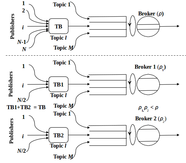
Figure 2: Alternative DRL configurations

2.1 Why splitting a token bucket is bad

In this section, we formally establish that distributing the rate limiting function across multiple token buckets, i.e., splitting them, has a negative impact on the (access) delay that the token bucket itself can introduce (what we termed the DRL penalty). In particular, even if message and token rates are perfectly matched at the sub-token buckets across brokers, the splitting alone ensures that messages experience a higher access (in the token bucket) delay. As alluded to earlier, this increase in access delay can all but offset the benefits of the greater message processing capacity afforded by having access to multiple brokers.

Towards establishing this, we derive the stronger result that splitting a token bucket into multiple sub-token buckets always increases the cumulative rate limiting delay that messages experience, irrespective of how messages are distributed across sub-token buckets. The result is formally stated in the next proposition whose proof can be found in Appendix A.

Proposition 1.

Given a two-parameter token bucket $(r,b)$ and a general message arrival process where messages each require one token to exit the bucket, splitting this one-bucket system into multiple, say, $k$, sub-token buckets with parameters $(r_{l},b_{l})$ such that $r=\sum_{l=1}^{k}r_{l}$ and $b=\sum_{l=1}^{k}b_{l}$, can never improve the running sum of the message delays, irrespective of how messages are distributed to the $k$ sub-token buckets. More generally, denoting as $S(t)$ and $S^{(k)}(t)$ the sum of the delays accrued by all messages up to time $t$ in the one-bucket and $k$-bucket systems, respectively, we have

$$S^{(k)}(t)\geq S(t)\,,\,\forall t$$

While general, the result provides little insight into its underlying cause. To develop such insight, we explore the special case of independent Poisson publishers for which the rate limiting delay can be explicitly expressed.

Let $\lambda$ denote the aggregate (Poisson) message arrival rate of a topic, and $(r,b)$ the parameters of its token bucket. Under the assumption of Poisson arrivals, the system behaves like a modified M/D/1 queue [16, 17] with a job arrival rate of $\lambda$ and a service time of $1/r$ (the time needed to generate one token), with messages delayed only when upon arrival the unfinished work $U$ in the M/D/1 system exceeds $b-1$. The expected delay in an $(r,b)$ token bucket is then of the form:

$$E[T_{TB}^{(1)}] = \frac{1}{2r}\cdot\frac{P_{\mbox{M/D/1}}(U>b-1)}{\left(1-\frac{\lambda}{r}\right)}$$ (1)

where $P_{\mbox{M/D/1}}(U>b-1)$ can be computed as shown in [40, Section 15.1] and captures the odds that a message is delayed in the token bucket while $\frac{1}{2r\left(1-\lambda/r\right)}$ is the expected delay of messages that have to wait for tokens.

Under Poisson arrivals, Eq. (1) still holds after (randomly) splitting messages across, say, $k$ brokers, with corresponding message arrival rates and sub-token bucket parameters that verify $\sum_{l=1,\ldots,k}\lambda_{l}=\lambda$, $\sum_{l=1,\ldots,k}r_{l}=r$, and $\sum_{l=1,\ldots,k}b_{l}=b$, where for ease of exposition, we assume that $\lambda/r=\lambda_{l}/r_{l},\forall\,l$, i.e., message and token rates are perfectly matched,

From Eq. (1), we can readily identify the two factors that contribute to the DRL penalty. Specifically,
(i) $P_{\mbox{M/D/1}}(U_{l}>b_{l}-1)\geq P_{\mbox{M/D/1}}(U>b-1)$: smaller buckets $(b_{l}\leq b)$ imply that messages are more likely to have to wait;
(ii) $\frac{1}{2r_{l}}>\frac{1}{2r}$: with lower token rates $(r_{l}\leq r)$, messages that have to wait (due to lack of tokens) wait longer.

Hence, Eq. (1) states that under the assumption of Poisson arrivals, splitting the token bucket $k$-ways yields at least a $k$-fold increase in access delay (e.g., assuming $r_{l}=\frac{r}{k},\forall\,l$), and likely more (because
$P_{\mbox{M/D/1}}(U_{l}>b_{l}-1)\geq P_{\mbox{M/D/1}}(U>b-1)$).

We note that the delay increase from the slower token rates $r_{l}$ is unavoidable and not dependent on the assumption of Poisson arrivals. On the other hand, the fact that $P_{\mbox{M/D/1}}(U_{l}>b_{l}-1)\geq P_{\mbox{M/D/1}}(U>b-1)$ is explicitly dependent on the assumption of a Poisson process hints at the possibility that for different arrival processes this penalty may not always arise, or may be mitigated by properly crafting the arrival process at each broker.

To better understand when and why this may be the case, consider a scenario where a token bucket $(r,b)$ is split in two equal sub-token buckets $(r/2,b/2)$. Assume now that instead of independent Poisson publishers, publishers are synchronized, i.e., generating messages at the same time to create an aggregate burst (batch Poisson). Splitting publishers equally across sub-token buckets then also splits the burst in the same proportion as the bucket size. All other parameters, e.g., load, being the same, $P(U_{2}>b/2-1)\approx P(U>b-1)$, and the odds of messages being delayed are mostly unchanged.

In the next section, we discuss how we translate this intuition into a set of principles aimed at mitigating the DRL penalty while meeting topics’ SLOs.

3 SRTM Goals and Principles

As reflected in LD, SRTM seeks to offer a messaging service (for IoT applications) that is both efficient in its use of cloud resources and capable of enforcing latency guarantees (SLOs). A common SLO is in the form of a tail latency guarantee, e.g., a $99^{\mbox{th}}$ percentile latency below $1$ ms. This calls for both controlling the messaging workload that originates from users (through rate limiting) and for determining how to best distribute that workload across message processing resources (brokers). As discussed in the previous section, the difficulty lies in the opposing effects of load distribution on message processing and rate limiting latency, respectively.

A tongue-in-cheek restatement of the challenge faced by DRL decisions would be “to split, or not to split?” Given the finding of Proposition 1, a natural guideline is to only split if you have to. In other words, distribute a topic’s publishers across the fewest brokers while ensuring that the resulting message processing loads do not result in SLO violations. Additionally, our intuition points to another postulate, namely, if you split the load, split the burst, at least to the extent possible. Specifically, publishers whose message transmission times tend to be correlated, and therefore contribute to forming a burst, should be assigned to different brokers.

Our approach to distributing publishers of a new topic to message brokers builds on this insight. Section 4 provides details on the resulting design, but we give next a brief overview and motivation for those choices. Specifically, SRTM incorporates three principles:

1. Concentration: Identify the smallest number of brokers needed to meet the new topic’s SLO;

2. Max-min: Maximize the minimum workload, and consequently token rate, assigned to any broker;

3. Correlation-awareness: Assign publishers to brokers to minimize inter-publisher correlation, and consequently reduce the burstiness of the message arrival process at each broker as much as possible.

Concentration directly derives from Proposition 1 that identifies that the DRL penalty is unavoidable. Hence, we seek to avoid or minimize it whenever feasible. In particular, as highlighted by Eq. (1), the DRL penalty can grow linearly and often super-linearly with the number of sub-token buckets across which the workload is split. Hence, it is natural to avoid splitting a topic as long as the broker’s load does not yield a processing latency that violates the topic’s SLO.

Max-min is similarly inspired by Eq. (1) and the fact that, irrespective of the arrival process, the access delay of messages that experience a delay is inversely proportional to the token rate. Hence, keeping the minimum token rate across sub-token buckets as high as possible is desirable for achieving tail latency guarantees.

Correlation-awareness seeks to select publishers so as to decrease the “burst” of the arrival process at each sub-token bucket in a manner that parallels the decrease in the size of their respective bucket size. We note that decreasing arrival bursts should benefit both the DRL penalty and the message processing delay in the brokers.

4 SRTM Design

This section presents the design of SRTM, with Fig. 3 offering a high-level overview of a typical configuration. The core component of SRTM is a Load Distributor which is responsible for distributing a topic’s publishers to brokers based on the topic’s SLO and the brokers’ existing workload. In addition, a TB Adaptor tracks the status of sub-token buckets at run time and triggers adjustments of their $(r_{l},b_{l})$ parameters in response to message traffic changes. In this section, we focus on the design of the SRTM Load Distributor, as it is the primary component responsible for realizing the principles put forth in Section 3. Other components, including the TB Adaptor, are detailed in Section 5.

4.1 Design Challenges

The Load Distributor is designed based on the three principles presented in Section 3. However, realizing them calls for addressing two practical challenges.

Estimating Capacity. In contrast to traditional load balancers SRTM does not seek to evenly distribute load across available resources. Instead, the Concentration principle calls for determining the smallest number of brokers that can accommodate a new topic subject to its SLO (tail latency target). This, and to a lesser extent the Max-min principle, is essentially an “admission control” problem, where the system keeps assigning publishers to a broker unless the topic’s SLO is violated. Admission control requires an accurate estimation of the number of publishers a broker can handle subject to the SLO.

In practice, estimating the broker capacity is challenging as message processing involves a set of inter-dependent and concurrent tasks. For example, the NSQ open-source messaging middleware [8] is implemented using the Go language (Golang) [10], which provides lightweight and scalable concurrency through Goroutines. This is well suited to IoT applications that involve large numbers of concurrent connections, and motivated our choice of NSQ as the basis for SRTM. However, modeling the behavior of the Goroutine runtime scheduler, including its reliance on a work-stealing strategy to exploit multicore systems, is non-trivial. Furthermore, depending on both the level of parallelism (number of publishers) of a topic and how publishers generate messages, performance bottlenecks migrate across NSQ components. This makes a model-based approach mostly impractical and leads us to instead rely on a measurement-based approach [19]. Specifically, we use iterative measurements to discover how to best distribute a topic’s publishers across brokers while meeting its latency target (see Section 4.2).

Accounting for Correlation. The other design challenge arises in realizing the correlation-awareness principle. Specifically, based on Eq. (1), given that a workload is to be split across a number of brokers, SRTM’s goal is to identify an assignment of publishers that results in the smallest possible increases in $P(U_{l}>b_{l}-1)$ across brokers. This means crafting an arrival process at each broker that achieves this goal. This is challenging as it requires precise temporal characterization of the workload generated by individual publishers.

A reasonable option is to minimize the inter-arrival time variance at each broker. However, crafting such an outcome from individual publisher arrival processes is computationally complex. Furthermore, variance only reflects global statistics of the arrival process at each broker, and so does not fully capture temporal correlation. Hence, minimizing variance needs not realize our goal of limiting increases in $P(U_{l}>b_{l}-1)$. Alternatives that rely on indices of dispersion [22, 27, 50] are equally if not more complex, as is directly measuring temporal correlation.

Those challenges lead us to instead rely on an altogether different alternative, namely, user-specified publisher correlation keys that reflect IoT application-level semantics (see Section 4.3 for details).

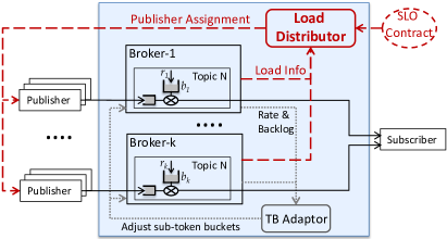
Figure 3: SRTM Architecture Overview.
The new topic (Topic N) is distributed across Broker-$1\sim k$

4.2 Iterative Workload Distribution

When a new topic arrives, the Load Distributor is responsible for distributing its publishers among brokers to meet the topic’s SLO. As discussed in Section 4.1, it is challenging to accurately estimate the number of publishers a broker can accommodate subject to an SLO. To overcome this challenge, the Load Distributor employs an iterative process that distributes publishers across brokers as part of a measurement-based profiling phase.

Each iteration of the load distribution process works as follows: (1) the Load Distributor first estimates the minimum number of brokers ($k$) with enough available capacity to accommodate the new topic; (2) the topic’s publishers are then assigned to the $k$ brokers in conformance with the max-min and correlation-awareness principles; (3) after publishers have been assigned to the $k$ brokers, each broker runs an independent profiling phase (measuring latency) to validate whether it can accommodate its new workload without violating its SLO.

After Step (3), each broker knows if it can handle its new workload or needs to shed some publishers to remain in compliance with its SLO. If there are no SLO violations, the load distribution process is deemed successful and ends. Otherwise, brokers whose SLO was violated determine how many publishers they need to shed, report this number to the Load Distributor, and mark themselves as “full.” The Load Distributor then starts a new iteration to distribute released publishers, possibly involving additional brokers. The process ends when all publishers are assigned to brokers that can accommodate them, or the system runs out of brokers. When that happens, more brokers may be spawn by issuing a request to the cloud.

Next, we describe each step in more details, with the exception of the correlation-aware assignment of publishers, which is the subject of its own sub-section, Section 4.3. For simplicity, we first describe the process used in the first iteration that takes place when a new topic arrives. We then extend the discussion by describing how the variables used in each iteration are updated.

Step (1) reflects our concentration goal and seeks to determine the minimum number of brokers needed to accommodate a new topic with a given aggregate message $rate$. The residual message processing capacity ($rcap$) of each broker is first estimated based on the difference between its maximum message processing capacity ($mcap$), and its currently allocated message rate (the sum of the message $rate$s from topics already assigned to the broker). Brokers are then sorted in decreasing order of $rcap$ value to identify the minimum initial number $k$ of brokers to which to assign the new topic’s workload (the smallest number of brokers such that the sum of their $rcap$ values exceeds the topic’s message rate).

Step (2) determines how to best distribute the message workload of the new topic across those $k$ brokers according to the max-min and correlation-awareness principles. This involves computing for each broker a workload $quota$ it should be assigned. This $quota$ is set to the minimum of the broker’s residual capacity $rcap$, and its fair share $rate/k$ of the workload. This maximizes the minimum assignment at each broker (the max-min principle), unless limited by residual capacity. Once $quotas$ are set, brokers $rcap$ values are updated to reflect their new allocation, and publishers are assigned to brokers to realize those allocations in a correlation-aware manner, which, as mentioned earlier, is described in Section 4.3.

Step (3) acknowledges that estimates for $rcap$ only account for message rates, and therefore ignore many factors that affect performance, e.g., arrival burstiness, concurrency (among connections from different publishers), interactions across workloads, etc. Step (3), therefore, relies on a measurement-based approach to evaluate the actual performance of each broker after Step (2).

Specifically, Step (3) includes a profiling phase, which we call online-fitting, whose goals are to (i) test whether each broker’s SLO is still met after adding the new publishers (by measuring end-to-end message latency), and (ii) if it is not, determine how many publishers the broker needs to shed to return to compliance with the SLO. Under (ii), an iterative binary search is triggered to identify the how many publishers the broker can accommodate without violating its SLO. Excess publishers are returned to the Load Distributor, with the broker marked as full.

This next iteration parallels the first one with updated variables. A new variable $ua\_rate$ records the aggregate unassigned message rate from excess publishers, while $k$ is increased to account for the smallest number of additional brokers needed to accommodate $ua\_rate$ in a manner that again conforms to the max-min and correlation-awareness principles. Iterations continue until all publishers are assigned to brokers that can accommodate them, or the system runs out of brokers.

In spite of its accuracy, we acknowledge that this iterative process has disadvantages. First, its measurement-based nature implies that convergence can take time. We quantify this in Section 6.5. Second, the SLO needs not be met while we iterate. This is unavoidable in any measurement-based approach and, as discussed in Section 4.1, is a consequence of the difficulties in constructing a sufficiently general and accurate model.

4.3 Correlation-aware Allocation

As pointed out in Section 4.1, measuring correlation across a topic’s publishers is challenging. As a result, we adopt a pragmatic approach where users provide correlation information based on application semantics commonly available in IoT settings. Our approach is inspired by the concept of partition keys used in stream processing in Azure IoT hub [15, p. $123$], which allows users to explicitly identify correlated data streams to facilitate efficient stream processing by jointly considering streams within the same partition. Partitions that give rise to temporal correlation among publishers are common in many IoT deployments. For example, sensors in close proximity to each others will often trigger around the same time when detecting the same physical phenomenon. Publishers associated with those sensors, will then produce correlated message arrival patterns to the messaging system.

We adapt the concept of partition keys in SRTM, and provide APIs to users that let them label correlated publishers with an identical correlation group key.

Returning now to the end of Step (2) of the workload distribution process, the Load Distributor seeks to assign publishers with the same correlation key to different brokers, thereby splitting the message “bursts” they jointly generate. Specifically, given a set of correlation groups (as specified by the user) and a number of publishers to be assigned to a broker (based on $rcap$ and $rate/k$), the Load Distributor selects publishers from each correlation group in proportion to the number of publishers in the group.

5 SRTM Implementation

As mentioned earlier, SRTM is based on NSQ. In this section, we first introduce NSQ’s architecture, and then present our approach to adding SRTM’s functionality together with some challenges we had to address. While discussions on implementation challenges are closely tied to NSQ, several of the issues we encountered are broadly applicable to systems that need to achieve predictable performance while relying on high concurrency platforms (for scalability) such as Go runtime.

5.1 NSQ Architecture Overview

As shown in Fig. 4, NSQ comprises a set of goroutines. Messages from publishers arrive on separate TCP connections each handled by an IOLoop goroutine. Messages from publishers of a given topic are then passed to another goroutine, Topic. The Topic goroutine has a dedicated buffer into which IOLoop goroutines move messages. Once a Topic goroutine is scheduled for execution, it runs to completion by pulling messages from its buffer and forwarding them to MsgPump goroutines until the buffer becomes empty. The MsgPump goroutines sends messages to subscribers through separate TCP connections. The Go runtime employs a work-stealing scheduler to schedule all the goroutines on multicore platforms. The lightweight goroutines and the scheduler are important to the scalability of NSQ that may need to handle a large number of publishers through a single broker.

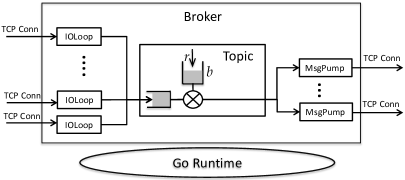
Figure 4: Goroutines in a NSQ broker

5.2 Rate Limiting

SRTM enforces rate limits through a token bucket that resides in the Topic goroutine. At runtime, each Topic goroutine keeps track of the state of its token bucket. When a Topic goroutine is scheduled, it pull messages from its incoming message buffer only if its token bucket has tokens. Otherwise, the routine returns and messages wait in the message buffer until tokens become available.

While the logic of a token bucket is well understood, it is non-trivial to implement its precise temporal behavior in a high concurrency environment such as Go runtime. Specifically, the token bucket determines whether a message is conformant based on its state (number of tokens) and the message arrival time. The straightforward approach to measure arrival times is to timestamp messages when the IOLoop goroutine reads them from the TCP receive buffer. However, because of the cooperative scheduling of goroutines, the times at which an IOLoop goroutine is scheduled to read messages can significantly differ from when messages are first received in the TCP buffer. As the token bucket logic updates its token count based on how much time has elapsed since the message arrived, a late arrival timestamp can cause the token bucket to mistakenly delay messages that are actually conformant. Such scheduling delays can become significant when the number of goroutines in the system is large. In particular, a topic with a large number of publishers, and consequently IOLoop goroutines, might introduce large temporal errors in the token bucket’s behavior.

To eliminate those errors, SRTM employs TCP-layer timestamping. The arrival of each TCP packet (sk_buff) is recorded inside the Linux kernel (in the tcp_v4_rcv function). Whenever an IOLoop reads data, the TCP arrival timestamps are also copied (as out-of-band data) to user space. As user data (messages) often do not map 1:1 to TCP packets (fragments), each IOLoop maintains a mapping between received messages and TCP packets and assigns each message the timestamp from the correct TCP packet. As arrival timestamps at the TCP-layer are independent of goroutine scheduling, SRTM is able to enforce rate limits with high temporal accuracy.

5.3 Handling Garbage Collection

Garbage Collection (GC) in the Go runtime can have a significant impact on the tail latency of message processing in NSQ. When GC is triggered, Go runtime uses marker goroutines to mark memory allocations, which can consume up to 25% of CPU time [32]. As a result, we found significant increases in the $99^{\mbox{th}}$ percentile in the message processing tail latency when GC is triggered.

As GC is usually triggered on demand in Go [7], we can minimize GC invocations by reducing dynamic memory allocation and hence slowing the growth of the heap size. We developed a GC-friendly version of NSQ by replacing instances of dynamic memory usage with statically allocated memory. Specifically, we created a pre-allocated ring buffer for each IOLoop, such that data read from the TCP socket is directly written into an existing slot in the ring buffer instead of having to request a dynamic memory allocation. In addition to on-demand GC, Go runtime forces GC if there is no GC in a $2$ minutes (by default) interval. We disabled this feature so that in SRTM, GC is solely triggered on demand. Although these optimizations do not completely eliminate the impact of GC, they effectively mitigate it for the $99^{\mbox{th}}$ percentile tail latency in our experiments.

5.4 Adapting to Workload Changes

As discussed in Section 4.2, SRTM performs load distribution upon the arrival of a new topic. Traffic may, however, shift over time across brokers, while remaining conformant to the global $(r,b)$ traffic profile. The resulting mis-match between traffic and sub-token buckets can then produce significant DRL penalties. To avoid this, SRTM’s static rate control configuration is augmented with a TB Adaptor that adjusts sub-token bucket parameters in response to “long-term” traffic shifts.

Specifically, every broker periodically reports to the TB Adaptor the rate and burst statistics of its topics. In our implementation, this is based on a per-topic 10s history window that tracks the average message rate and maximum backlog over that window in 1s increments. The TB Adaptor adjust token rates in proportion to average message rates, and token bucket sizes in proportion to maximum backlogs. To balance responsiveness and stability, SRTM administrators can adjust the length of the history window and the frequency of updates.

Note that the TB Adaptor only adjusts sub-token bucket parameters to avoid DRL penalties caused by shift in traffic among publishers. This does not address problems that may arise when a shift in traffic overloads a broker. Handling such scenarios calls for the ability to migrate publishers among brokers. Although this feature has been implemented (and is used in the profiling phase), its introduction as a runtime mechanism is left as future work.

6 Evaluation

This section presents an empirical evaluation of SRTM, and more precisely of the different design principles on which it relies. Section 6.1 starts with experiments designed to illustrate the impact of DRL on tail latency, while Sections 6.2 to 6.4 proceed with quantifying the relative benefits derived from each one of SRTM’s three principles. This is realized through a progression of designs that incorporate SRTM’s principles one at the time. Finally, Section 6.5 explores a more pragmatic aspect, namely, the amount of time SRTM takes to converge to a stable load distribution after the arrival of a new topic.

Testbed. The evaluation is carried out on a testbed consisting of 7 physical hosts. Fig. 5 offers an overview of the testbed. Hosts boast two 8-core Intel Xeon E5-2630 processors, 8 GB of memory, and are connected by 40 Gbps Ethernet links. Hosts $1,2$ and $3,4$ are dedicated to publishers and subscribers, respectively. There are $6$ brokers in total, deployed over Hosts $5$ and $6$. Each broker has $2$ dedicated CPU cores, which is also the default CPU configuration of Amazon-MQ instances [1]. The Load Distributor and TB Adaptor are deployed at Host $7$.

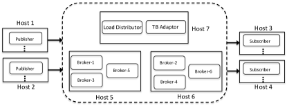
Figure 5: Testbed Setup

Workload. We generate a messaging workload that seeks to mimic IoT traffic. In a typical IoT setup, messages for a topic originate from multiple publishers, with publishers corresponding to a single sensor or a gateway aggregating a group of sensors. Messages can be time-triggered or event-triggered. Time-triggered messages are usually generated periodically. For example, intelligent transportation systems may require periodic traffic updates from sensors across a city [4, 9]. Conversely, event-triggered messages are generated upon detecting specific environmental changes. For example, building thermostats may trigger when temperature drops below (or exceeds) a certain threshold.

We emulate time-triggered traffic with publishers sending messages periodically. Because we were unable to secure real-world traces of event-triggered messages, we approximated the resulting traffic using a Poisson process (randomly occurring events). Both periodic and Poisson publishers may generate messages in a batch, with the batch size determining the traffic burstiness. For example, a gateway controlling a group of sensors would generate a batch of messages if the sensors are controlled by a common timer or triggered by the same event.

We selected a $99^{\mbox{th}}$ percentile end-to-end message latency of $1ms$ as the SLO across all experiments. Whenever a given design is unable to meet the $1ms$ SLO, we report the performance of the best configuration. Additionally, topics’ token buckets were configured using a profiling phase that gathered a representative traffic trace. The trace was used to perform an offline simulation of the token bucket performance using a token rate $r$ set $10\%$ higher than the topic’s message rate, and searching for the smallest bucket size $b$ that ensured a $99^{\mbox{th}}$ percentile token bucket access delay of zero.

6.1 Illustrating the DRL Penalty

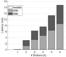
(a) 1,000 publishers

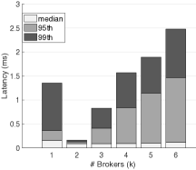
(b) 6,000 publishers

Figure 6: DRL penalty for Poisson workloads
(10 msg/s per publisher – batch size of 1).

This section explores the impact of the DRL penalty on tail latency through two experiments (see Fig. 6) that differ in their message workload. In both experiments, the publishers of a new topic have access to the $6$ brokers, which for consistency are initially all idle. The first experiment illustrates the DRL penalty when the topic’s load is low, i.e., a single broker is nominally able to accommodate the topic. The second experiment considers a heavier load for which a trade-off arises between access to more capacity when spreading the load across brokers vs. the resulting increase in DRL penalty. Both experiments rely on publishers that generate single messages (batch size of $1$) according to a Poisson process of rate of $10\leavevmode\nobreak\ msg/s$.

The first experiment involves a topic with $1,000$ (Poisson) publishers (a workload of $10,000\leavevmode\nobreak\ msg/s$) that are distributed across 1 to 6 brokers, with the topic’s token bucket correspondingly split among them. Fig. 6a shows the median, $95^{\mbox{th}}$, and $99^{\mbox{th}}$ percentile of the end-to-end latency for the 6 configurations. It illustrates the increase of the $99^{\mbox{th}}$ percentile latency with the number of brokers across which the topic is split (it reaches $14.7ms$ for $k=6$). This is because in low load configurations, as is the case here, the benefit from access to more broker capacity is small and does not offset the DRL penalty.

The second experiment (Fig. 6b) is similar except that it now uses $6,000$ publishers. The higher message rate overloads a single broker, as illustrated by the case $k=1$ that exhibits a large tail latency. Splitting publishers between two brokers reduces the tail latency, as the decrease in message processing latency (from the lower broker load) exceeds the increase in DRL penalty (from splitting the token bucket). Distributing the topic across more brokers is, however, of no benefit, as the increase in DRL penalty again exceeds the decrease in message processing latency. This highlights the trade-off that Fig. 2 alluded to.

Next, we compare SRTM against a series of baseline solutions that incrementally incorporate the design principles behind SRTM, namely, concentration, max-min, and correlation-awareness. The experiments allow us to isolate the contributions of each principle, while assessing their overall impact when combined in SRTM.

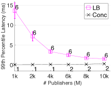
(a) Poisson, Batch=1,

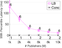
(b) Poisson, Batch=10,

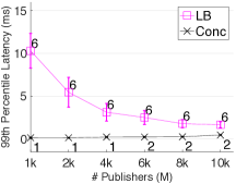
(c) Periodic, Batch=1,

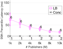
(d) Periodic, Batch=10,

Figure 7: Impact of Concentration on $99^{\mbox{th}}$ percentile Latency. (Batch: batch size per publisher; average message rate per publisher: 10 message/s.)

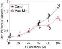
(a) Poisson, Batch=1

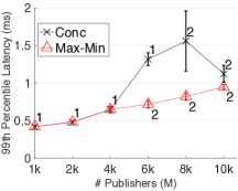
(b) Poisson, Batch=10

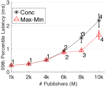
(c) Periodic, Batch=1

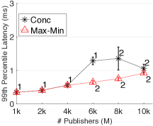
(d) Periodic, Batch=10

Figure 8: Impact of Max-Min on $99^{\mbox{th}}$ percentile Latency.
Initial (Poisson) load on brokers 1-6 (in kmsg/s): 10, 40, 50, 60, 70, 80 (w/ batch size of 10 messages).

6.2 The Benefits of Concentration

In this section, we evaluate the impact of concentration by comparing a baseline approach, Load Balancing (LB), that evenly distributes a topic’s publishers across all available brokers, to an alternative, Conc, that incorporates the concentration principle. Conc distributes publishers across brokers so as to equalize the total load on each broker, but unlike LB that carries this distribution out across all brokers, it limits itself to the smallest possible number of brokers the topic requires. This number is first estimated based on the topic’s message rate and brokers’ $rcap$ values, and then validated using a measurement-based approach as described in Section 4.2.

The comparison is carried out for different workloads by varying the number of publishers associated with a topic. As before, publishers have a fixed message rate of $10\leavevmode\nobreak\ msg/s$, and we again consider Poisson and periodic publishers. We vary the burstiness of the message generation process of each publisher by changing the size of the message batch they generate (1 or 10). Periodic publishers are independent of each other, with a randomly selected phase for their period. Experiment start again with idle brokers and are repeated $10$ times. The results are shown in Fig. 7 with the mean and standard deviation of the $99^{\mbox{th}}$ percentile latency reported for each configuration. The number of brokers across which the topic’s workload is distributed is also shown next to each data point.

Figs. 7a and 7b report the results for Poisson publishers and batch sizes of $1$ and $10$, respectively, with Figs. 7c and 7d devoted to periodic publishers. Results are qualitatively consistent across scenarios, and illustrate the benefit of the concentration principle (Conc meets the topic’s SLO for all configurations, while LB consistently fails to). The figures also highlight two relatively intuitive factors.

The first is the impact of the aggregate message rate on the DRL penalty. Specifically, as the number of publishers, and therefore the topic’s aggregate message rate, increases, the penalty that LB incurs decreases. A return to Eq. (1) readily explains why. A higher token rate means a smaller token generation time (service time), and consequently a shorter delay as is well-known from basic queueing theory. Hence, while the DRL penalty is still present, a high message rate means that the token rate at each broker even after splitting the traffic 6 ways (as LB requires) remains high enough to ensure a comparatively small penalty relative to the message processing delay.

The other factor the figures bring to light is how traffic burstiness amplifies the DRL penalty. This can again be explained by looking at Eq. (1). When applied to a batch (Poisson) arrival process, the bucket size and the token rate are scaled down by the batch size, which both contribute to an increase in delay (the last message in a batch of size $10$ that finds an empty token bucket waits for $10$ tokens). It is this “amplification” factor that is behind the significantly worse performance of LB for batch arrivals.

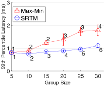
(a) Poisson Topic

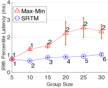
(b) Periodic Topic

Figure 9: Impact of Correlation-aware Allocation.
(Each publisher has a batch size of 10 and an average message rate of 10/s; Topic has 1,000 publishers).

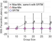
(a) Poisson Topic

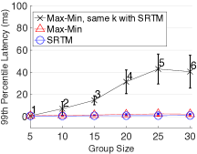
(b) Periodic Topic

Figure 10: Impact of Correlation-aware Allocation.
(Max-Min uses the same number of brokers as SRTM).

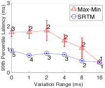
(a) Poisson

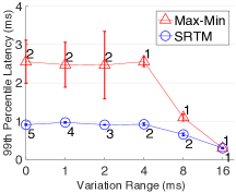
(b) Periodic

Figure 11: Latency evaluation - imprecise correlation.
(Each publisher has a batch size of 10 and an average message rate of 10/s; Topic has 1,000 publishers).

6.3 The Benefits of Max-Min

To evaluate the impact of the max-min principle, we reuse the scenarios of the previous section, but assume that a new topic finds brokers with varying pre-existing message loads (as shown in the caption of Fig. 8). We also introduce a new baseline algorithm, Max-Min, that extends Conc by incorporating the max-min principle. As Conc, Max-Min targets accommodating the new topic with the smallest possible number of brokers, but instead of aiming to equalize the total load at each broker, it seeks to maximize the minimum topic load assigned to a broker.

Figs. 8a and 8b compare Conc and Max-Min for a new topic with Poisson publishers, while Figs. 8c and 8d report similar results for periodic publishers. The presence of existing workloads on the $6$ brokers affects the new topic’s distribution across brokers as a function of its own workload. When it is low, it can fit on the most lightly loaded broker and Conc and Max-Min perform identically. Their performance, however, starts deviating as the topic’s load increases (beyond 4k publishers) and needs to be split over multiple brokers. For example, when the topic boasts 8k publishers, it now needs to be distributed across brokers 1, 2, and 3. Conc equalizes the total load of the three brokers, while Max-Min instead seeks to maximize the topic’s load on broker $3$ that, because it has the heaviest existing load, receives the smallest share. This results in a $99^{\mbox{th}}$ percentile latency of $1.50ms$ for the publishers assigned to broker $3$ under Conc, while it is $0.87ms$ under Max-Min, and the difference primarily arises from the larger DRL penalty under Conc.

As the two sets of figures show, Poisson and periodic publishers yield similar outcomes, but the experiments also reveal an interesting yet ultimately intuitive behavior when it comes to the impact of burstiness in the topic’s arrival process. In particular, Figs. 8c and 8d display performance for a new topic with publishers that generate bursts of $10$ messages, and both Conc and Max-Min perform as well if not better as when publishers generate bursts of size $1$. This initially counter-intuitive behavior is because, in this scenario, the performance of the new topic is dominated by the processing of the IOLoop goroutines associated with its publishers (recall the overview of Section 5.1). Under a bursty arrival process, a publisher’s IOLoop is scheduled less frequently, which results in a smaller number of simultaneously active IOLoops that need to be serviced by the Go runtime scheduler. This results in a broker being able to handle a higher overall message load under both Max-Min than Conc, simply from the smaller number of IOLoops from the new topic.

Another interesting behavior that Figs. 8c and 8d reveal is the improvement in performance of Conc when the new topic goes from 8k to 10k publishers. The reason is again differences in DRL penalty. With 8k publishers, the “left-over” number of publishers assigned to the second broker is smaller than with 10k publishers, and consequently the resulting DRL penalty is higher. This illustrates the primary weakness of relying on concentration only, as it can result in residual assignments to the last broker that produce very high DRL penalties. Again, this is the primary motivation behind the Max-Min principle.

6.4 The Benefits of Correlation Awareness

As discussed in Section 4.3, correlation in how publishers generate messages is captured through correlation groups. We then compare Max-Min to SRTM that incorporates group information when distributing publishers across brokers (Max-Min is oblivious to that information, while SRTM seeks to leverage it to distribute publishers across brokers so as to reduce arrival burstiness in proportion to the reduction in bucket size). Towards isolating the impact of correlation, we again assume that a new topic arrives to a set of idle brokers.

Additionally, because correlation groupings can be coarse, e.g., reflecting physical proximity rather than precise synchronization, we consider two scenarios. The first assumes that publishers within the same group are perfectly correlated, i.e., their message generation times are precisely synchronized, while the second relaxes this assumption by introducing variations in the times at which publishers in the same group generate messages.

6.4.1 Scenario $1$: Accurate correlation

In this set of experiments, publishers marked as belonging to the same group are perfectly synchronized in their message generation times. We vary group sizes across experiments, with larger groups corresponding to larger (synchronized) message bursts generated by each group. The main consequence of such an increase is that meeting the $1ms$ SLO for burstier traffic calls for distributing the topic across more brokers. This affects both Max-Min and SRTM, but the fact that SRTM relies on group information to split publishers from the same group across brokers enables it to mitigate the resulting increase in DRL penalty.

The results are shown in Figs. 9a and 9b for Poisson and periodic publishers, respectively. Both figures illustrate that SRTM is able to gain access to more broker capacity (and break message bursts) without incurring a significant increase in DRL penalty. This allows it to meet the target SLO, even for groups of size $30$. In contrast, Max-Min is forced to use fewer brokers, as its “blind” assignment of publishers ultimately results in a DRL penalty that exceeds the benefits of distributing the topic’s message load across more brokers. This is further illustrated in Fig. 10 that also reports the performance of Max-Min when it tries to use the same number of brokers as SRTM. As anticipated, this makes its performance even worse.

6.4.2 Scenario $2$: Noisy correlation

This next set of experiment is explores the extent to which the benefits of a correlation-aware distribution of publishers remain when correlation information is inaccurate. Specifically, the message generation times of publishers within the same group are now (evenly) spread over an interval instead of perfectly concurrent. As the interval size increases, correlation between publishers weakens.

Results are reported in Fig. 11 that compares SRTM and Max-Min, again for both Poisson and periodic publishers. The experiments relied on the same type of publishers as in the previous section with a group size set to $25$, and the interval across which messages from the same group were distributed ranged from $0ms$ to $16ms$ ($0ms$ corresponds to the configuration of the previous section). The results are again consistent for both Poisson and periodic publishers and demonstrate that, at least when the level of noise is small (of the order of a few percent of the average message inter-arrival time), leveraging correlation information still helps mitigate the DRL penalty. The figure also illustrates another side-effect of increasing the size of the interval over which publishers’ messages arrive, namely tail latency as well as the number of brokers across which publishers are distributed decrease for both SRTM and Max-Min. This behavior is a direct consequence of the lower burstiness associated with the increased “spreading” of message arrivals.

6.5 Load Distribution Latency

As described in Section 4.2, SRTM uses only the broker’s average message load to estimate the residual capacity $rcap$ available on each broker. This simple approach is because the complex internal architecture of NSQ makes accurately modeling the impact of higher order arrival statistics challenging if not impossible. As a result, SRTM resorts to a measurement-based solution to “fine-tune” its initial (imprecise) capacity estimates and the resulting publishers to brokers allocations. This fine-tuning is carried out in the online-fitting component of Step $(3)$ of the load distribution mechanism. As previously mentioned, a potential disadvantage is that such an approach can take time to converge. Gaining insight into this load distribution latency is the purpose of this section.

Before reporting the results of those experiments, we however highlight that significant improvements are possible if topics’ workloads are limited to a few well-understood traffic profiles for which customized models can be developed (as may be the case for specific applications). Such specialization is, however, beyond the scope of this paper, and instead we proceed next to quantify the load distribution latency in one illustrative configuration.

Specifically, we consider scenarios involving a new topic arriving to a set of empty brokers. This latter assumption arguably simplifies the load distribution process, as the brokers are homogeneous in their spare capacity. Nevertheless, the basic steps of SRTM’s load distribution remain present. The topic’s message load stands at a relatively low level of $10k\leavevmode\nobreak\ msg/s$ ($1,000$ publishers, each with a message rate of $10\leavevmode\nobreak\ msg/s$ and a burst size of 10), and we vary its burstiness by changing the publishers’ group size (publishers in a group are perfectly synchronized). When burstiness is low (small group size), a single broker is able to accommodate the new topic, but as burstiness increases, so does the number of brokers needed, with $6$ brokers eventually required when the group size reaches $30$.

Because the topic’s workload is low and brokers are initially empty, the first $rcap$-based assignment always starts with $k=1$ (a single broker is deemed to have enough capacity). Depending on the topic’s burstiness, additional brokers may, however, be needed (resulting in an increase in $k$). This is reflected in the different rows of Table 1, where each row corresponds to a different level of burstiness, and within a given row, a column ($k$ value) represents one iteration of Step $(3)$ of the load distribution.

An iteration starts with an assignment of publishers to a broker and seeks to assess if the SLO is met. If it is, the load distribution process successfully completes. If it is not, a binary search is initiated to determine the maximum number of publishers the broker can accommodate. Entries in the table give the number of search rounds. Each round lasts $60$ secs to ensure a representative traffic sample and are the primary contributors to load distribution latency, whose total value is reported in the last column. Once the number of publishers a broker can accommodate has been identified, excess publishers are then assigned to the next broker and $k$ is increased by $1$.

We note that because brokers are initially idle, iterations always proceed one broker at the time, with each broker fully loaded before the next one is added, i.e., we never have to consider shifting excess publishers to previously considered brokers. This is also why the last iteration completes in a single round.

Table 1 indicates that as the burstiness (group size) of the topic increases, so does the duration of the load distribution phase. This is expected, since our estimate of $rcap$ is oblivious to workload burstiness, and therefore becomes less accurate as it increases. For bursty topics, initial assignments systematically over-estimate the number of publishers a broker can accommodate. This triggers repeated iterations, each calling for a binary search. In the “worst” case (group size of 30), the cumulative effect of those searches results in a load distribution phase in excess of $15$ minutes. This is clearly long, though not unreasonable when dealing with, say, an IoT deployment that may last for weeks or months. Additionally and as mentioned earlier, if variations in traffic profile parameters can be constrained, better models for estimating $rcap$ are feasible and would reduce the number of iterations.

Group Size	$k$ $=1$	$k$ $=2$	$k$ $=3$	$k$ $=4$	$k$ $=5$	$k$ $=6$
5	1
10	2	1
15	5	3	1
20	5	4	2	1
25	3	4	4	2	1
30	3	5	3	2	3	1

Time (sec)
64
189
558
745
871
1058

Table 1: Load distribution latency of SRTM
$k$: iteration index; each $k$ column gives the number of measurement rounds in that iteration; the last column reports the total load distribution time.

7 Related Work

On the system side, distributed rate limiting (DRL) has been realized in a number of cloud services through software platforms such as Cloud Bouncer [5], Tyk [13] and Doorman [6]. Those platforms provide coordination protocols that set rate limiting parameters across resources as a function of a global contract and workload partitions.

Also relevant to our work are approaches that dynamically adapt control decisions across distributed resources based on a global objective. Raghavan et al. [38] describe a system of (distributed) rate limiters that drop packets probabilistically to emulate the effect of a single aggregate rate limiter on transport layer congestion. Retro [34] proposes a resource management framework that can enforce objectives such as fairness or latency guarantees by dynamically adapting resource allocation across multiple systems and tenants. It relies on a centralized controller coupled to a measurement infrastructure and distributed control points. Stanojevic et al. [44, 43] develop analytical models that account for both load balancing and rate limiting in determining how to optimally control access to distributed resources as a function of demand. The goal is to realize a fair outcome while incurring a low computational and communication overhead.

As alluded to in Section 1.1, the primary difference between those works and the approach we adopt is that they seek to replicate the behavior of a centralized system in spite of their distributed nature, while we instead acknowledge the impact of distribution (the DRL penalty) and attempt to mitigate it. Either approach has its own merit with benefits that vary as a function of the environment in which it is deployed. We believe that the mostly static partitioning of resources on which we rely affords robustness in settings where adaptation latency is large compared to the time-scale of workload dynamics.

Another related body of work targets the same concentration principle as SRTM, but to reduce operational or energy costs while meeting SLOs. WorkloadCompactor [51] explores how to best shape (through token buckets) co-located workloads with latency constraints to maximize the number of workloads that a server can accommodate. A similar cost reduction goal is behind the use of concentration in STeP [45] that realizes it by co-locating tenants with compatible resource usage patterns. Other systems [48, 23, 20, 31] realize a similar goal by co-locating latency-sensitive workloads with data-intensive (batch-processing) workloads. In spite of similarity in the end-goal (concentration), our goal of seeking it to mitigate the DRL penalty differs from that of those earlier works.

Similarly, load-balancing strategies are common in distributed cloud services. The objective is to evenly distribute an aggregate load across servers to optimize performance given an available set of servers. Load-balancers [21, 14, 26, 37] can therefore be effective in minimizing processing latency. However, as illustrated in Fig. 2 and demonstrated in Fig. 6, a strict load-balancing strategy can be counter-productive in the presence of a DRL penalty. This is true even when combining it with concentration, which motivated the introduction of the Max-Min principle in SRTM.

Finally, leveraging workload correlation to improve system performance has been the focus of a number of earlier works, which have typically relied on traces to capture correlation in resource usage. For example, STeP [45] used FFT co-variance to reduce CPU contention by co-locating anti-correlated databases. Power consumption was the target of Verma et al. [47] that proposed to consolidate anti-correlated applications based on Pearson correlation, and of Carpo [49] that also relied on Pearson correlation to consolidate loosely-correlated flows in data center networks. Although SRTM shares with those works a reliance on correlation to optimize performance, it differs in both the performance metric it targets (the DRL penalty) and its approach to measuring correlation (using IoT application semantics rather than measurements).

8 Conclusion

The paper’s main contributions are in identifying and explicating the DRL penalty that unavoidably arises when rate control is distributed across servers, and in designing and developing a system, SRTM, capable of mitigating this penalty with a focus on its use by IoT applications.

The SRTM system relies on three core principles: concentration, max-min and correlation-awareness, and was evaluated empirically on a local testbed. The evaluation demonstrated its ability to successfully mitigate the DRL penalty, while preserving the ability to scale by distributing workload across servers when needed. SRTM was developed on top of the NSQ open-source messaging platform and is publicly available for others to use [42].

SRTM is fully operational, but relies on a measurement-based solution to accurately match arbitrary workload to system resources. This matching can in some cases be time-consuming. A promising extension for configurations involving more specialized workloads involves developing an accurate model-based resource matching solution that would overcome this limitation.

Appendix A Rate Limiting Delay

A.1 Model and Assumptions

Consider a two-parameters token bucket [28] $(r,b)$ where $r$ denotes the token rate (in messages/sec) and $b$ the allowed burst size (in messages). In other words the number of messages that can leave the token bucket in any time interval of duration $\Delta t$ (the arrival curve to the system downstream of the token bucket) is upper-bounded by $b+r\cdot\Delta t$. Message arrivals to the token bucket follow an arbitrary arrival process and each message consumes one token. Messages that find an available token upon their arrival immediately clear the token bucket without incurring any delay. Messages that arrive to an empty token bucket (or a token bucket with only a fraction of a token) wait until a full token is available before they are allowed to leave the token bucket. The waiting space at the token bucket is assumed large enough (infinite) to ensure that messages waiting for tokens are never lost.

Of concern are delays incurred in the token bucket, i.e., the rate limiting delays. Our focus is on the sum $S(t)$ of the delays accrued by all message up to time $t$. In particular, we are interested in the impact on $S(t)$ of replacing a one-bucket system $(r,b)$ with a two (or more) bucket system consisting of two separate sub-token buckets $(r_{1},b_{1})$ and $(r_{2},b_{2})$, where $r=r_{1}+r_{2}$ and $b=b_{1}+b_{2}$. In the two-bucket system, the original stream of arrivals is split arbitrarily across the two sub-token buckets at the times of message arrivals, and each sub-token bucket has an infinite queue where messages waiting for tokens can be stored.

We note that under the assumptions of a general message arrival process with each message requiring exactly one token, a token bucket system with unit token rate, i.e., $r=1$, and a bucket size of $b$ tokens behaves like a modified G/D/1 queue with unit service times. The modification is that in the token bucket system, messages experience a delay if and only if the queue content in the G/D/1 system exceeds $b-1$. In other words, assuming a first-served-first-come (FCFS) order of service, the token bucket delay $d_{i}$ of the $i^{th}$ message can be obtained from the system time of this message in the corresponding G/D/1 system as follows:

$$d(a_{i})=\max\{0,U(a_{i}^{-})+1-b\}\,,$$ (2)

where $U(a_{i}^{-})+1$ corresponds to the unfinished work found in the G/D/1 queue by the $i^{th}$ message upon its arrival at time $a_{i}$ plus its own contribution to the unfinished work, and $b$ is the bucket size.

Next, we proceed to compare the relative (latency) performance of a one-bucket system to that of a multi-bucket system obtained by splitting the one-bucket system as described above. In particular, we establish that splitting a token bucket in two (or more) sub-token buckets always increases the sum of the message delays, and hence also the average message delay.

A.2 One vs. Two or more Token Buckets

Towards establishing the result that splitting a token bucket can only worsen the sum of message delays, we first state a simple Lemma.

Lemma 2.

At any point in time $t$, the unfinished work $U(t)$ in a work-conserving G/D/1 queue is smaller than or equal to the total unfinished work $U^{(k)}(t)=\sum_{l=1}^{k}U_{l}(t)$ in a set of $k$ work-conserving G/D/1 queues with the same aggregate service rate and fed the same arrival process.

Proof.

The result directly stems from the observation that when fed the same arrival process, $k$ parallel work-conserving G/D/1 queues never clear work faster than a single work-conserving G/D/1 queue with the same aggregate service rate. Specifically, at any point in time both the one-queue and the $k$-queues system have received the same amount of work (they are fed the same set of arrivals), both systems are work-conserving, and the one-queue system processes work at least as fast as the $k$-queue system whenever it is not empty, so that it can never have more unfinished work than the $k$-queue system.

Formally, we assume that up to the start of the $j^{th}$ busy period of the one-queue system, the unfinished work in the one-queue system has always been smaller than or equal to that of the $k$-queue system, and wlog we assume that the one-queue system has unit service rate. We establish the result by induction on the busy periods of the one-queue system.

Denote as $t_{j}$ the start of the $j^{th}$ busy period of the one-queue system, and let $T_{j}$ denote the duration of that busy period. The unfinished work in the one-queue system during that busy period is then of the form $U(t)=U(t_{j}^{-})+W(t_{j},t)-(t-t_{j})=W(t_{j},t)-(t-t_{j})\,,\,\forall t\in[t_{j},t_{j}+T_{j}]$, where $W(t_{j},t)$ represents the amount of work that has arrived in $[t_{j},t]$, and we have used the fact that by definition the unfinished work just before the start of a busy period is $0$. Similarly, the unfinished work in the $k$-queue system is of the form $U^{(k)}(t)=U^{(k)}(t_{j}^{-})+W(t_{j},t)-\int_{t_{j}}^{t}r^{(k)}(u)du\geq W(t_{j},t)-(t-t_{j})=U(t)\,,\,\forall t\in[t_{j},t_{j}+T_{j}]$, where we have used the facts that $U^{(k)}(t_{j}^{-})\geq U(t_{j}^{-})=0$ (from our induction hypothesis), $r^{(k)}(u)\leq 1$, i.e., the aggregate service rate in the $k$-queue system can never exceed the unit service rate of the one-queue system, and both systems receive the same amount of work $W(t_{j},t)$. Furthermore, because by definition of a busy period $U(t_{j}+T_{j})=0$ and both the one-queue and the $k$-queue system see the same arrivals, we also have $0=U(t)\leq U^{(k)}(t)\,,\,\forall t\in[t_{j}+T_{j},t_{j+1})$, where $t_{j+1}$ is the start time of the $(j+1)^{th}$ busy period of the one-queue system, i.e., the time of the next arrival after $t_{j}+T_{j}$. This establishes that the unfinished work in the one-queue system remains smaller than or equal to that in the $k$-queue system until the start of the $(j+1)^{th}$ busy period of the one-queue system. This completes the proof of the induction step. ∎

We are now ready to prove Proposition 1, which we restate next for completeness.

Proposition 1 Given a two-parameter token bucket $(r,b)$ and a general message arrival process where messages each require one token to exit the bucket, splitting this one-bucket system into multiple, say, $k$, sub-token buckets with parameters $(r_{l},b_{l})$ such that $r=\sum_{l=1}^{k}r_{l}$ and $b=\sum_{l=1}^{k}b_{l}$, can never improve the running sum of the message delays, irrespective of how messages are distributed to the $k$ sub-token buckets. More generally, denoting as $S(t)$ and $S^{(k)}(t)$ the sum of the delays accrued by all messages up to time $t$ in the one-bucket and $k$-bucket systems, respectively, we have

$$S(t)\leq S^{(k)}(t)\,,\,\forall t$$ (1)

Proof.

We first establish the result for the case $k=2$, and wlog assume that $r=1$.

The proof is simply based on the fact that messages waiting for tokens in either system accrue delay at the same rate, and establishing that at any time $t$ the number $N(t)$ of messages experiencing delays in the one-bucket system is less than or equal to the number $N_{1}(t)+N_{2}(t)$ of such messages in the two-bucket system. Note that the sum of the message delays incurred in either system up to time $t$ is of the form

$$S(t) = \int_{0}^{t}N(u)du$$

$$S^{(2)}(t) = \int_{0}^{t}\left(N_{1}(u)+N_{2}(u)\right)du$$

Hence, if $N(t)\leq N_{1}(t)+N_{2}(t)\,,\,\forall t$, then $S(t)\leq S^{(2)}(t)\,,\,\forall t$, which proves the result for $k=2$. We therefore proceed to establish that $N(t)\leq N_{1}(t)+N_{2}(t)\,,\,\forall t$.

The number $N(t)$ of messages waiting for tokens, i.e., accruing delay, at time $t$ in a one-bucket system with bucket size $b$ is of the the form

$$N(t)=\left\lceil\max\{0,U(t)-b\}\right\rceil\,,$$

where $\lceil x\rceil$ represents the ceiling of $x$, $U(t)$ is the unfinished work in the corresponding G/D/1/ queue, and consistent with Eq. (2) we have used the fact that messages are delayed in the token bucket only when the unfinished work in the G/D/1 queue exceeds the bucket size $b$.

Similarly the total number of messages waiting for tokens in a two-bucket system with bucket sizes $b_{1}$ and $b_{2}$ such that $b=b_{1}+b_{2}$ is of the form

$$N_{1}(t)+N_{2}(t)=\left\lceil\max\{0,U_{1}(t)-b_{1}\}\right\rceil+\left\lceil\max\{0,U_{2}(t)-b_{2}\}\right\rceil$$

Since we know that $\lceil x\rceil\leq\lceil x_{1}\rceil+\lceil x_{2}\rceil$, when $x\leq x_{1}+x_{2}$, we focus on establishing that

$$\max\{0,U(t)-b\}\leq\max\{0,U_{1}(t)-b_{1}\}+\max\{0,U_{2}(t)-b_{2}\}$$ (3)

From Lemma 2, we know that $U(t)\leq U_{1}(t)+U_{2}(t)$. Next, we consider the cases $U(t)-b\leq 0$ and $U(t)-b>0$.

Case $1$: $U(t)-b\leq 0$

In this case, Eq. (3) is trivially verified.

Case $2$: $U(t)-b>0$

We further separate this case in two separate sub-cases:

Case $2a$: $U_{1}(t)-b_{1}\leq 0$ and $U_{2}(t)-b_{2}\geq 0$ (or interchangeably $U_{1}(t)-b_{1}\geq 0$ and $U_{2}(t)-b_{2}\leq 0$)

In this case, Eq. (3) simplifies to

$$U(t)-b\leq U_{2}(t)-b_{2}$$

Applying again the result of Lemma 2, we have

$$U(t)\leq U_{1}(t)+U_{2}(t)\, \Rightarrow\,U(t)-b\leq U_{1}(t)+U_{2}(t)-b_{1}-b_{2}$$

$$\Rightarrow\,U(t)-b\leq U_{2}(t)-b_{2}\,,$$

where we have used the fact that $b=b_{1}+b_{2}$ and $U_{1}(t)-b_{1}\leq 0$. Hence, Eq. (3) again holds in Case $2a$.

Case $2b$: $U_{1}(t)-b_{1}\geq 0$ and $U_{2}(t)-b_{2}\geq 0$

In this case, Eq. (3) becomes

$$U(t)-b\leq U_{1}(t)-b_{1}+U_{2}(t)-b_{2}\,,$$

which again holds because of Lemma 2 and the fact that $b=b_{1}+b_{2}$.

Since the case $U_{1}(t)-b_{1}\leq 0$ and $U_{2}(t)-b_{2}\leq 0$ is not possible under Case $2$ (it would violate Lemma 2), this establishes that Eq. (3) holds in all cases. Accordingly, $N(t)\leq N_{1}(t)+N_{2}(t)\,,\,\forall t$, so that as mentioned earlier, $S(t)\leq S^{(2)}(t)\,,\,\forall t$, which establishes the result for $k=2$.

Extending the result to $k>2$ is readily accomplished by applying the above approach recursively to groups of two sub-token buckets. ∎

In concluding, we note that while Eq. (2) assumed an FCFS service ordering for messages in the token bucket, both Lemma 2 and Proposition 1 are independent of the order in which messages waiting for tokens are scheduled for transmission, as long as the schedule is “work-conserving,” i.e., (waiting) messages in any bucket leave as soon as one full token is available.

References

- [1] Amazon MQ. https://aws.amazon.com/amazon-mq/.
- [2] AWS IoT Core. https://aws.amazon.com/iot-core/.
- [3] Azure IoT Hub. https://azure.microsoft.com/en-us/services/iot-hub/.
- [4] CityPulse. http://www.ict-citypulse.eu/page/.
- [5] Cloud Bouncer: Distributed Rate Limiting at Yahoo. https://yahooeng.tumblr.com/post/111288877956/cloud-bouncer-distributed-rate-limiting-at-yahoo.
- [6] Doorman. https://github.com/youtube/doorman.
- [7] Golang Package Debug: SetGCPercent. https://golang.org/pkg/runtime/debug.
- [8] NSQ. http://nsq.io/.
- [9] SCATS. http://www.scats.com.au/.
- [10] The Go Programing Language. https://golang.org/.
- [11] Throttle API Requests for Better Throughput. https://docs.aws.amazon.com/apigateway/latest/developerguide/api-gateway-request-throttling.html.
- [12] Transform and Protect your API. https://docs.microsoft.com/en-us/azure/api-management/transform-api.
- [13] Tyk: Rate limiting. https://tyk.io/docs/control-limit-traffic/rate-limiting/.
- [14] T. Barbette, C. Tang, H. Yao, D. Kostić, G. Q. M. Jr., P. Papadimitratos, and M. Chiesa. A High-Speed Load-Balancer Design with Guaranteed Per-Connection-Consistency. In Proceedings of the 17th USENIX Symposium on Networked Systems Design and Implementation (NSDI 20), pages 667–683, Santa Clara, CA, Feb. 2020.
- [15] A. Basak, K. Venkataraman, R. Murphy, and M. Singh. Stream Analytics with Microsoft Azure. Packet Publishing, Ltd., 2017.
- [16] A. W. Berger. Performance analysis of a rate-control throttle where tokens and jobs queue. IEEE J. Select Areas Comm., 9(2):165–170, February 1991.
- [17] A. W. Berger and W. Whitt. The impact of a job buffer in a token-bank rate-control throttle. Stochastic Models, 8(4):685–717, 1992.
- [18] A. Botta, W. de Donato, V. Persico, and A. Pescapé. Integration of cloud computing and Internet of Things: A survey. Future Generation Computer Systems, 56:684–700, 2016.
- [19] L. Breslau, S. Jamin, and S. Shenker. Comments on the performance of measurement-based admission control algorithms. In Proceedings of IEEE INFOCOM 2000, volume 3, pages 1233–1242 vol.3, 2000.
- [20] E. Cortez, A. Bonde, A. Muzio, M. Russinovich, M. Fontoura, and R. Bianchini. Resource Central: Understanding and Predicting Workloads for Improved Resource Management in Large Cloud Platforms. In Proceedings of the 26th Symposium on Operating Systems Principles, SOSP ’17, page 153–167, New York, NY, USA, 2017.
- [21] D. E. Eisenbud, C. Yi, C. Contavalli, C. Smith, R. Kononov, E. Mann-Hielscher, A. Cilingiroglu, B. Cheyney, W. Shang, and J. D. Hosein. Maglev: A Fast and Reliable Software Network Load Balancer. In Proceedings of the 13th USENIX Symposium on Networked Systems Design and Implementation (NSDI 16), pages 523–535, Santa Clara, CA, Mar. 2016.
- [22] K. W. Fendick and W. Whitt. Measurements and approximations to describe the offered traffic and predict the average workload in a single-server queue. Proceedings of the IEEE, 77(1):171–194, January 1989.
- [23] A. Goder, A. Spiridonov, and Y. Wang. Bistro: Scheduling Data-Parallel Jobs Against Live Production Systems. In Proceedings of the 2015 USENIX Annual Technical Conference (USENIX ATC 15), pages 459–471, Santa Clara, CA, July 2015.
- [24] M. P. Grosvenor, M. Schwarzkopf, I. Gog, R. N. M. Watson, A. W. Moore, S. Hand, and J. Crowcroft. Queues Don’t Matter When You Can JUMP Them! In Proceedings of the 12th USENIX Symposium on Networked Systems Design and Implementation (NSDI 15), pages 1–14, Oakland, CA, May 2015.
- [25] K. Grünberg and W. Schenck. A case study on benchmarking iot cloud services. In International Conference on Cloud Computing, pages 398–406. Springer, 2018.
- [26] A. Gulati, G. Shanmuganathan, I. Ahmad, C. Waldspurger, and M. Uysal. Pesto: Online Storage Performance Management in Virtualized Datacenters. In Proceedings of the 2nd ACM Symposium on Cloud Computing, SOCC ’11, New York, NY, USA, 2011.
- [27] R. Gusella. Characterizing the variability of arrival processes with indices of dispersion. Technical Report TR-90-051, International Computer Science Institute, September 1990.
- [28] J. Heinanen and R. Guerin. A Single Rate Three Color Marker. RFC 2697 (Informational), Sept. 1999.
- [29] C. N. Hoefer and G. Karagiannis. Taxonomy of cloud computing services. In Proc. IEEE Globecom Workshops, Miami, FL, December 2010.
- [30] K. Jang, J. Sherry, H. Ballani, and T. Moncaster. Silo: Predictable Message Latency in the Cloud. In Proceedings of the 2015 ACM Conference on Special Interest Group on Data Communication, SIGCOMM ’15, page 435–448, New York, NY, USA, 2015.
- [31] S. A. Javadi, A. Suresh, M. Wajahat, and A. Gandhi. Scavenger: A Black-Box Batch Workload Resource Manager for Improving Utilization in Cloud Environments. In Proceedings of the ACM Symposium on Cloud Computing, SoCC ’19, page 272–285, New York, NY, USA, 2019.
- [32] W. Kennedy. Garbage Collection In Go : Part I - Semantics. https://www.ardanlabs.com/blog/2018/12/garbage-collection-in-go-part1-semantics.html.
- [33] K. Lan, Z. Wang, M. Hassan, T. Moors, R. Berriman, L. Libman, M. Ott, B. Landfeldt, and Z. Zaidi. Experiences in deploying a wireless mesh network testbed for traffic control. ACM SIGCOMM Computer Communication Review, 37(5):17–28, 2007.
- [34] J. Mace, P. Bodik, R. Fonseca, and M. Musuvathi. Retro: Targeted resource management in multi-tenant distributed systems. In Proceedings of the 12th USENIX Conference on Networked Systems Design and Implementation, NSDI ’15, pages 589–603, USA, 2015.
- [35] S. Mao and S. Panwar. A survey of envelope processes and their application in quality of service provisioning. IEEE Communications Surveys, 8(3), 3rd Quarter 2006.
- [36] Microsoft. Partitioned Queues and Topics. https://docs.microsoft.com/en-us/azure/service-bus-messaging/service-bus-partitioning.
- [37] N. Park, I. Ahmad, and D. J. Lilja. Romano: Autonomous Storage Management Using Performance Prediction in Multi-Tenant Datacenters. In Proceedings of the Third ACM Symposium on Cloud Computing, SoCC ’12, New York, NY, USA, 2012.
- [38] B. Raghavan, K. Vishwanath, S. Ramabhadran, K. Yocum, and A. C. Snoeren. Cloud Control with Distributed Rate Limiting. SIGCOMM Comput. Commun. Rev., 37(4):337–348, Aug. 2007.
- [39] J. Rao. How to choose the number of topics/partitions in a Kafka cluster. https://www.confluent.io/blog/.
- [40] J. Roberts, U. Mocci, and J. Virtamo, editors. Broadband Network Teletraffic – Final Report of Action COST 242. Springer, 1996.
- [41] M. Rubinovitch. The slow server problem. Journal of Applied Probability, 22(1):205–213, March 1985.
- [42] SRTM: A scalable real-time messaging service. To be added. Removed for anonymity.
- [43] R. Stanojevic and R. Shorten. Generalized distributed rate limiting. In Proceedings of the 17th International Workshop on Quality of Service, pages 1–9, 2009.
- [44] R. Stanojevic and R. Shorten. Load Balancing vs. Distributed Rate Limiting: An Unifying Framework for Cloud Control. In Proceedings of the 2009 IEEE International Conference on Communications, pages 1–6, 2009.
- [45] R. Taft, W. Lang, J. Duggan, A. J. Elmore, M. Stonebraker, and D. DeWitt. STeP: Scalable Tenant Placement for Managing Database-as-a-Service Deployments. In Proceedings of the Seventh ACM Symposium on Cloud Computing, SoCC ’16, page 388–400, New York, NY, USA, 2016.
- [46] N. Uuganbaatar. Optimality of first-come-first-served: a unified approach. Mongolian Mathematical Journal, 15:45–53, 2011.
- [47] A. Verma, G. Dasgupta, T. K. Nayak, P. De, and R. Kothari. Server Workload Analysis for Power Minimization Using Consolidation. In Proceedings of the 2009 Conference on USENIX Annual Technical Conference, USENIX’09, page 28, USA, 2009.
- [48] A. Verma, L. Pedrosa, M. Korupolu, D. Oppenheimer, E. Tune, and J. Wilkes. Large-Scale Cluster Management at Google with Borg. In Proceedings of the Tenth European Conference on Computer Systems, EuroSys ’15, New York, NY, USA, 2015.
- [49] X. Wang, Y. Yao, X. Wang, K. Lu, and Q. Cao. Carpo: Correlation-aware power optimization in data center networks. In Proceedings of the 2012 IEEE INFOCOM, pages 1125–1133, 2012.
- [50] W. Whitt and W. You. The advantage of indices of dispersion in queueing approximations. Operations Research Letters, 47(2):99–104, March 2019.
- [51] T. Zhu, M. A. Kozuch, and M. Harchol-Balter. WorkloadCompactor: Reducing Datacenter Cost While Providing Tail Latency SLO Guarantees. In Proceedings of the 2017 Symposium on Cloud Computing, SoCC ’17, page 598–610, New York, NY, USA, 2017.