We consider a short rollercoaster cosmology based on two stages of monodromy inflation separated by a stage of matter domination, generated after the early inflaton falls out of slow roll. If the first stage is controlled by a flat potential, $V\sim\phi^{p}$ with $p<1$ and lasts ${\cal N}\sim 30-40$ efolds, the scalar and tensor perturbations at the largest scales will fit the CMB perfectly, and produce relic gravity waves with $0.02~{}\mbox{\raisebox{-2.58334pt}{$\stackrel{{\scriptstyle<}}{{\sim}}$}}~{}r~{}\mbox{\raisebox{-2.58334pt}{$\stackrel{{\scriptstyle<}}{{\sim}}$}}~{}0.06$, which can be tested by LiteBIRD and CMB-S4 experiments. If in addition the first inflaton is strongly coupled to a hidden sector $U(1)$, there will be an enhanced production of vector fluctuations near the end of the first stage of inflation. These modes convert rapidly to tensors during the short epoch of matter domination, and then get pushed to superhorizon scales by the second stage of inflation, lasting another $20-30$ efolds. This band of gravity waves is chiral, arrives today with wavelengths in the range of $10^{8}$ km, and with amplitudes greatly enhanced compared to the long wavelength CMB modes by vector sources. It is therefore accessible to LISA. Thus our model presents a rare early universe theory predicting several simultaneous signals testable by a broad range of gravity wave searches in the very near future.

1 Introduction

Inflation [1, 2, 3] arose as a paradigm to explain the universe naturally. It has been noted well prior to its advent that the universe is incredibly unnatural at the largest scales [4]. Without accelerated expansion early on, generic initial conditions would have yielded a far less hospitable universe, which raised the questions of fine tuning and anthropic selection early on. The mechanism of inflation addresses these problems by reducing the sensitivity to the initial conditions, metaphorically taking the log of the measure of tuning: one needs a total of $\sim 60$ efolds to shield from bad influences of initial anisotropies and inhomogeneities. As a bonus one receives a mechanism to generate structures at shorter scales, using local and causal dynamics enshrined in the effective field theory (EFT) of the inflaton sector.

Thus inflation translates the problem of cosmological naturalness to the problem of naturalness of the inflaton EFT. The construction of natural EFTs is relatively straightforward in the limit of semiclassical gravity. For example, all one needs is a single field with a flat potential and derivative couplings to everything else, and a model is born [5]. However with full-on quantum gravity, building UV complete inflation models is quite challenging. One general approach which was initiated in the past decade or so is monodromy inflation [6, 7, 8, 5], where the natural EFTs of the inflaton can be protected from the perils of quantum gravity by embedding them into gauge theories spontaneously broken at some scale above the scale of inflation, but below the fundamental gravity scale.

Even so, deploying monodromy models is nontrivial, with some pressure coming from both the theory side due to backreaction induced in setups with large field variations, and the observations, because the dynamics predicts large amplitude primordial gravity waves. We stress that backreaction is not automatically detrimental, since corrections often turn beneficial by flattening inflaton potentials and prolonging inflation instead of shortening it [9, 10, 11, 12]. The flatter potentials however tend to make the spectral index bluer. This seems to narrow the remaining theory space for these models.

In this Letter we argue that such a view is far too pessimistic. Within the recently expounded framework of rollercoaster cosmology [13] (see also [14, 15, 16, 17, 18, 19]), monodromy models remain completely viable, fitting the observations perfectly while relaxing the theoretical pressure from large field variations. More importantly, they are very predictive, producing primordial gravity waves within reach of both the future CMB searches such as LiteBIRD and CMB-S4, and the shorter scale instruments such as LISA. The reason is that the early stage of inflation can be completely interrupted, ending with a rapid reheating and then followed by another stage involving a completely different, second inflaton [13].

If the first stage lasts some $30$ – $40$ efolds, the flattened monodromy models with $V\sim\phi^{p}$, $p\lesssim 1/2$ [9, 10, 11, 12] easily produce the spectra of scalar and tensor perturbations completely within the current observational limits, with $n_{s}\sim 0.965$ and $r~{}\mbox{\raisebox{-2.58334pt}{$\stackrel{{\scriptstyle<}}{{\sim}}$}}~{}0.06$ (depending on $p$ and number of efolds, we can have a slightly larger upper bound for $r$). The flattening of the potential reduces $r$. Since the predictions are calculated at the pivot point of $N\sim 30$ – $40$ efolds before the end of the first stage of inflation, $n_{s}$ is more red. Hence both $n_{s}$ and $r$ move towards the observationally favored regime. Note also that the flattening dynamics which generates very shallow potentials activates other irrelevant operators, including higher derivative corrections to EFT [9, 10, 11, 12]. These terms yield equilateral nongaussianity $f_{NL}^{eq}\simeq{\cal O}(1)$ at CMB scales [12], again potentially accessible to detection. This also yields a lower bound on $r$, which makes the models quite predictive. Note further that additional stronger nongaussianities can be produced at shorter scales, during the interruption between the two stages of inflation, when the fields turn in the field space [20] (see [21] for an extensive review). Those are however not directly observable at present.

Further, since the inflatons are axions, they generically come from dimensional reduction of higher rank forms which have anomalous couplings. As a result the UV completion of inflatons yields the usual dimension-5 operators $\propto\phi F_{\mu\nu}\tilde{F}^{\mu\nu}/f$ in four dimensions, where $\tilde{F}_{\mu\nu}=\epsilon_{\mu\nu\lambda\sigma}F^{\lambda\sigma}/2$. When the field $\phi$ depends on time, such as an inflaton in the early stage, and the time dependence is reasonably fast, such as near the end of the first stage of inflation, one of the gauge field helicities becomes tachyonic at large wavelengths [22] and the tachyonic instability leads to a rapid, nonperturbative generation of the field $F$. In turn $F$ sources chiral gravity waves [23, 24] with an amplitude much greater than the non-chiral gravity waves generated by the standard metric fluctuations [25, 26, 13]. The dominant chiral gravity waves become superhorizon just before the end of the first stage of inflation, and their enhanced amplitude remains frozen during the short epoch of matter domination preceding the second stage of inflation, which provides additional $20$ – $30$ efolds [13]. During the last stage, the wavelength of the frozen chiral tensors stretches to the range of $10^{8}$ km which make them accessible to LISA.

Thus it would appear that the issues normally interpreted as theoretical challenges to inflation might instead be viewed as aspects of naturalness influenced by quantum gravity. Quantum gravity forces a modification of the flat space naturalness arguments; however the effect of these modifications need not be detrimental. On the contrary, monodromy inflatons with restricted field range, due to e.g. strong coupling effects, nevertheless naturally realize long inflation by using multiple inflatons working in unison. It turns out that in this sense these models are not only natural, but also more predictive than uninterrupted inflation, yielding detectable signals over a broad range of wavelengths.

2 Whither Double-coaster?

In the rest of this work we will specialize to a simple two-field model in which inflation is realized in two stages, connected by a phase during which the original inflaton field oscillates, so that the effective equation of state of the universe is approximately $w=0$, like CDM. Such models naturally occur in monodromy constructions, involving multiple fields with little hierarchies between their masses, and flattened effective potentials at large field ranges. The two-field potential we use is

$$V(\phi_{1},\phi_{2})=M_{1}^{4}\left[\left(1+\frac{\phi_{1}^{2}}{\mu_{1}^{2}}\right)^{\frac{p_{1}}{2}}-1\right]+M_{2}^{4}\left[\left(1+\frac{\phi_{2}^{2}}{\mu_{2}^{2}}\right)^{\frac{p_{2}}{2}}-1\right]\,.$$ (1)

The scales $\mu_{1},\mu_{2}$ normalizing the fields are both $\mathcal{O}(0.1M_{\mathrm{Pl}})$. We take $M_{2}~{}\mbox{\raisebox{-2.58334pt}{$\stackrel{{\scriptstyle<}}{{\sim}}$}}~{}M_{1}$.

Here we assume both fields $\phi_{i}$ are axions arising from truncating $p$-form gauge potentials in string theory compactifications. This immediately gives the mass scales $\mu_{i}\sim f_{i}$ linked to the axion decay constants. These in turn are bounded by $f\sim M_{Pl}/(M_{s}L)^{q}\lesssim M_{Pl}$ where $L$ is the size of the compactification cycle giving rise to the relevant axion, and $M_{s}$ the string scale [27, 28]. Hence, $f_{i}$ typically fall in the range $10^{-2}M_{Pl}\lesssim f\lesssim M_{Pl}$, justifying our choice of $\mu_{i}$. The scales $M_{i}$ typically arise from warping effects or dilution of energy densities with inverse powers of extra dimension volumes (see e.g. section 4.1 in [29] for a summary). These are either power-law and/or exponentially sensitive to the underlying microscopic parameters of a string compactification, and the axions $\phi_{i}$ arise from two different sectors of a given model. Hence generically $M_{1}\neq M_{2}$ and thus without loss of generality $M_{2}~{}\mbox{\raisebox{-2.58334pt}{$\stackrel{{\scriptstyle<}}{{\sim}}$}}~{}M_{1}$.

These choices decouple the early inflationary trajectory from the late inflationary dynamics. Therefore we can study the dynamic as a sequence of two consecutive single-field stages. We can view this as a very simple realization of Nflation [30], with a larger mass gap between the two inflatons, where one originally dominates but falls out of slow roll well before the other field does. The potential is illustrated in Fig. 1.

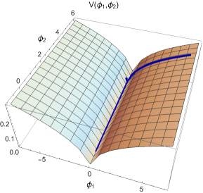
Figure 1: Two-field potential $V(\phi_{1},\phi_{2})$ for the model in eq. (1). Here $M_{1}=0.5M_{\mathrm{Pl}}$, $M_{2}/M_{1}=0.1$, $p_{1}=2/5$, $p_{2}=1$, $\mu_{1}=\mu_{2}=0.5$. The blue curve depicts a typical two-stage inflationary trajectory, where the field $\phi_{1}$ slides down the slope first, oscillates while decaying near the bottom of the “gutter”, and then $\phi_{2}$ starts to move along the “gutter”.

First, we determine the spectrum of perturbations on large scales. To do so, we solve the equations of motion for the inflaton and calculate the scalar spectral index $n_{s}$ and the tensor-to-scalar ratio $r$ at $N_{e}$ efolds before the end of the first stage, when the scales we see today in the Cosmic Microwave Background (CMB) and Large Scale Structure (LSS) leave the horizon. This means, we are using the effective potential during the first stage

$$V_{eff}(\phi_{1})=M_{1}^{4}\left[\left(1+\frac{\phi_{1}^{2}}{\mu_{1}^{2}}\right)^{\frac{p_{1}}{2}}-1\right]\simeq M_{1}^{4}\left[\left(\frac{\phi_{1}}{\mu_{1}}\right)^{p_{1}}-1\right]\,,$$ (2)

which in the plot of Fig. 1 corresponds to fixing $\phi_{2}$ at some value and rolling down the hill towards the ridge at a $\phi_{2}\simeq{\rm const.}$, thanks to $\phi_{2}\gg\mu_{2}$. Explicitly, we define the end of the first stage by $\epsilon=-\dot{H}/H^{2}\simeq 1$, which corresponds to roughly $\phi_{1}(end)\simeq\mu_{1}$ for our values of $\mu_{k}$, and use the slow-roll expressions $n_{s}-1=2\eta_{V}-6\epsilon_{V}$, $r=16\epsilon_{V}$ where $\epsilon_{V}=\partial_{\phi}V_{eff}(\phi_{1})^{2}/(2V_{eff}(\phi_{1})^{2})$, $\eta_{V}=\partial_{\phi}^{2}V_{eff}(\phi_{1})/V_{eff}(\phi_{1})$, calculated at a value of $\phi_{1}$ when

$$N_{e}=\int_{\phi_{1}}^{\phi_{1}(end)}d\phi\,\frac{H}{\dot{\phi}}\simeq\left(\frac{\phi_{1}^{2}}{2p_{1}M_{Pl}^{2}}\right)\left[1-\frac{2}{2-p_{1}}\left(\frac{\mu_{1}}{\phi_{1}}\right)^{p_{1}}\right]\,$$ (3)

efolds before the end of the first inflationary stage. As $\mu_{1}$ decreases, $N_{e}$ increases for fixed $p_{1}$ and $\phi_{1}$. At a first glance this might look surprising since $V_{eff}$ increases as $\mu_{1}$ decreases. However, as $\mu_{1}$ is scaled down the field ventures to flatter regions, and hence inflation runs longer. So the spectral index shifts slightly towards less red values. With the hierarchy between inflaton scales, this suppresses nongaussianities during the initial stage since the dynamics is dominated by one of the inflatons, such that its trajectory is almost straight in the field space [20]. We solve the equations numerically.

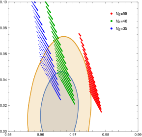
Figure 2: Tensor-to-scalar ratio versus spectral index for double monodromy, compared to the data of [31]. We show predictions for the parameter ranges $0.01\leq\mu_{1}\leq 1$, $0.1\leq p_{1}\leq 1$. The lines in the direction of decreasing $r$ and increasing $n_{s}$ correspond to varying $\mu_{1}$ at fixed $p_{1}$; as $\mu_{1}$ decreases, $N_{e}$ is larger since the potential is flatter at a fixed $\phi$ and so $n_{s}$ increases. This also lowers $r$ since a flatter potential implies a smaller $\epsilon$. The lines at approximately constant $n_{s}$ correspond to varying $p_{1}$ at fixed $\mu_{1}$. The important point however is that since the efold clock resets at the end of first stage, $n_{s}$ starts out smaller, and hence is slightly redder than in smooth inflation, fitting the data better. This is seen by the comparison of the three cases $N_{e}=35,40,55$ (where $N_{e}=55$ uses a single stage of uninterrupted inflation).

The results are shown in Fig. 2. We display our results similarly to [29], plotting predictions for different choices of parameters, at three choices of efolds before the end of the first stage of inflation: $N_{e}=55,40,35$. It is apparent that double monodromy inflation is fully compatible with the data. An interesting prediction of this whole class of models is that $r~{}\mbox{\raisebox{-2.58334pt}{$\stackrel{{\scriptstyle>}}{{\sim}}$}}~{}0.02$, which is well within the reach of near future B-modes searches (see, e.g. [32]).

Restricting $\Delta\phi$’s to be at most a few $M_{Pl}$, as per the current lore about large field variations (e.g. [33, 34, 35]), we see that the individual stages are pretty short. For example, for $x=\phi_{max}/M_{Pl}\sim 2$ – $3$, and with our values of $\mu$, Eq. (3) yields $N_{max}\simeq\left(\frac{x^{2}}{2p}\right)\left[1-\frac{1}{1-p/2}\left(\frac{1}{2x}\right)^{p}\right]$. For e.g. $p\sim 0.1$ these initial values readily yield $N_{max}\sim 20$ – $45$, and $\Delta\phi$ during inflation is at most $2$ – $3\,M_{Pl}$ only. With slightly larger $p$ the stages of inflation are shorter. Assuming a uniform distribution of field values, it is quite generic to obtain a multistage model which, with initial value of $\phi$’s saturating at $\phi_{max}$ will yield a longer earlier stage and a shorter later stage, realizing a double-coaster of $\sim 40$ and $\sim 20$ stages separated by a brief epoch of matter domination supported by the decay of the early inflaton. The price to pay is to arrange for the right combination of values of $p_{k},\mu_{k},M_{k}$, which seems readily attainable.

Note that in the first stage, the primordial spectrum of tensors remains at $r~{}\mbox{\raisebox{-2.58334pt}{$\stackrel{{\scriptstyle<}}{{\sim}}$}}~{}0.06$ at all scales at which the metric fluctuates, by scale invariance. The transition between different stages of inflation would not suddenly make this contribution jump up at shorter scales as noted by [25, 26, 13]. This opens the door for the nonperturbative generation of chiral tensors, using vector tachyon instability [23, 24]. We now turn to this mechanism.

3 Für LISA

Axion inflatons generically couple to $U(1)$ gauge fields via the standard dimension-5 operators $\propto\phi_{1}F_{\mu\nu}\tilde{F}^{\mu\nu}/2$. This can be seen in a particularly simple way in flux monodromy models [8, 36, 5]. Imagine that the axion sector arises from a dimensional reduction of, say, a $4$-form field strength in $11D$ Sugra, which has Chern-Simons self-couplings. Ignoring the volume moduli, and imagining a toroidal compactification for simplicity, we see that the $11D$ Lagrangian upon dimensional reduction and truncation to zero modes yields

$$-F_{abcd}^{2}+\epsilon_{a_{1}\ldots a_{11}}A^{a_{1}\ldots}F^{a_{4}\ldots}F^{a_{8}\ldots a_{11}} \ni -F^{2}_{\mu\nu\lambda\sigma}-(\partial\phi_{1})^{2}-\mu\phi_{1}\epsilon_{\mu\nu\lambda\sigma}F^{\mu\nu\lambda\sigma}$$ (4)

$$-\sum_{k}F^{2}_{\mu\nu\,(k)}-\frac{\phi_{1}}{f_{\phi}}\sum_{k,l}\epsilon_{\mu\nu\lambda\sigma}F^{\mu\nu}{}_{(k)}F^{\lambda\sigma}{}_{(l)}\,,$$

where the first line involves the $4$-form-axion sector, and the second the mixing of the axion with the $U(1)$ coming from the reduction of $F_{abcd}$. Here, $A_{abc}$ is the $3$-form potential, $F=dA$. The dimensional normalizations come from different scaling dimensions of various spins, and emerge after the size of internal cycles are accounted for [37]. After rotating modes in the $U(1)$ isospace and canonically normalizing the $4D$ fields, we see that $\phi_{1}$ will couple to at least one $4D$ $U(1)$ vector field. For simplicity, we take only one coupling to be nonzero, and model it with the canonically normalized $4D$ dimension-5 operator

$$\mathcal{L}_{\rm int}=-\sqrt{-g}\frac{\phi_{1}}{4f_{\phi}}F_{\mu\nu}\tilde{F}^{\mu\nu}\,,$$ (5)

where $f_{\phi}$ is sub-Planckian, and generically of the order of GUT scale (see e.g. [27, 28]). A rolling axion triggers the tachyonic instability of one circular polarization of the gauge field [22], whose exponential production both backreacts on the inflaton and produces scalar and tensor perturbations [23, 24]. A very comprehensive analysis of these effects was provided recently in [38]. The dynamics is governed by [38]

$$\ddot{\phi}_{1}+3H\dot{\phi}_{1}+\partial_{\phi_{1}}V(\phi_{1})-\frac{1}{f_{\phi}}\langle\vec{E}\cdot\vec{B}\rangle=0\,,$$

$$3H^{2}=\frac{\dot{\phi}_{1}^{2}}{2}+V(\phi_{1})+\frac{1}{2}\rho_{EB}\,,$$ (6)

$$A^{\prime\prime}_{\pm}(\tau,\vec{k})+\left[k^{2}\pm 2\lambda\xi kaH\right]A_{\pm}(\tau,\vec{k})=0\,,$$

where the dot denotes a derivative w.r.t. $t$, and the prime is a derivative w.r.t. to conformal time $\tau$. The $U(1)$ ‘electric’ and ‘magnetic’ fields are defined as usual in the Coulomb gauge, $\vec{E}=-\frac{1}{a^{2}}\frac{\mathrm{d}\vec{A}}{\mathrm{d}\tau}$, $\vec{B}=\frac{1}{a^{2}}\vec{\nabla}\times\vec{A}$, and $\rho_{EB}=(\vec{E}^{2}+\vec{B}^{2})/2$ is the standard U(1) energy density. We picked the usual circular helicity basis for $\vec{A}$ in (6). Further $\lambda$ is the sign of $\dot{\phi}_{1}$ and $\xi=\frac{1}{2f_{\phi}}\frac{d\phi_{1}}{dN_{e}}$, where $N_{e}$ is the efold clock reading, for notational convenience.

The key ingredient here is the vector field equation. Clearly, if $\dot{\phi}_{1}=0$, it reduces to the standard harmonic oscillator, where there is no particle production, and the initial population dilutes, with physical $\vec{E}$ and $\vec{B}$ fields diluting as $1/a^{2}$. On the other hand, when $\dot{\phi}_{1}\neq 0$, and for $2\xi>k/(aH)$, the gauge field helicity $-\lambda$ behaves like a tachyon, and is exponentially produced by the evolution of $\phi_{1}$ [39]. This is the case during inflation. Approximating slow roll with a patch of de Sitter where $\xi\simeq{\rm const}.$ yields

$$A_{-\lambda}(\tau,\vec{k})=\frac{e^{\pi\xi/2}}{\sqrt{2k}}W_{-i\xi,1/2}(2ik\tau)\,,$$ (7)

where $W_{k,m}(z)$ is the Whittaker function, and we have imposed the Bunch-Davies vacuum initial conditions. While this approximation is valid, the average energy density of this field, and its Chern-Simons term, can be estimated as, for $\xi\geq 3$,

$$\rho_{EB}=\langle\frac{E^{2}+B^{2}}{2}\rangle\simeq 1.3\cdot 10^{-4}H^{4}\frac{e^{2\pi\xi}}{\xi^{3}}\,,~{}~{}~{}~{}~{}~{}~{}~{}~{}\langle\vec{E}\cdot\vec{B}\rangle\simeq-2.4\cdot 10^{-4}\lambda H^{4}\frac{e^{2\pi\xi}}{\xi^{4}}\,.$$ (8)

We plot the evolution of $\rho_{EB}$ towards the end of the first inflationary stage, in Fig. 3.

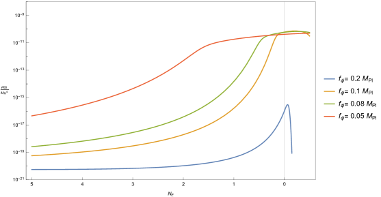
Figure 3: Evolution at the end of the first inflationary stage of the energy density in gauge fields, eq. (8). We denote by $N_{e}$ the number of efolds before the end of the first stage of inflation, and we normalize the energy density to $M_{\mathrm{Pl}}^{4}$. The parameters of the potential are fixed for convenience to $M_{1}^{4}=2\times 10^{-9}M_{\mathrm{Pl}}^{4}$, $\mu_{1}=M_{\mathrm{Pl}}$, $p=2/5$; at the CMB scales they lead to similar results as $\mu_{1}=0.1M_{\mathrm{Pl}}$, which fit CMB perfectly. We show results for different couplings $f_{\phi}$ as shown in the legend. The vertical line denotes the end of inflation, and the solutions we show are not completely reliable there. Note that the contributions of the vector field are very small until the very end of inflation, when $\phi_{1}$ moves the fastest. As a result the U(1) production does not affect CMB significantly.

The amplification of the vector field is bounded. First, the instability is driven by the slow roll – the tachyon is an instability of the transient background, not of the fundamental theory – and so the total energy deposited in the gauge field cannot exceed the inflaton kinetic energy. In particular, as inflation ends and $\phi_{1}$ settles into its minimum, the approximations (7) and (8) will cease to apply, with (7) reducing to the standard harmonic oscillator, as we noted above. We will take the transition from one limit to another to occur close to $\epsilon=-\dot{H}/H^{2}\sim 1$, or in other words, near the end of inflation, when $\dot{\phi}_{1}$ is almost maximal. This sounds counterintuitive, but from there on $\phi_{1}$ is decaying to its minimum, passing through zero quickly, and completely invalidating the approximations of (7), (8). At this point we will stop the numerical integration. Secondly, while the approximations (7) and (8) are valid, the U(1) vector gauge field energy density will backreact on the background evolution and the system will reach some equilibrium [39, 40]. This does not significantly modify early inflation. In particular, Fig. 2 remains valid as a prediction: early on the metric perturbations dominate over the vector-induced gravity waves, since the inflaton is deep in slow roll, and inflation is still going on. Essentially, this is just decoupling in action.

Towards the end of the first stage of inflation, as the field $\phi_{1}$ starts to move faster, the larger $\dot{\phi}_{1}$ results in a dramatic amplification of $\rho_{EB}$ cranking up the field strengths by as much as $\sim 10^{4}-10^{8}$, depending on the value of $f_{\phi}$. However the approximations break down at the exit of inflation, when $\rho_{EB}\sim\dot{\phi}_{1}^{2}/2$ by energy conservation, and instead the growth in the plots turns around, “plateauing” near the end of inflation [38]. While we do not zoom in on the specifics of this behavior here, the “plateau” at the end of inflation in Fig. 3 is interspersed with characteristic features since as the field $\phi_{1}$ starts to decay and oscillate, the tachyonic instability of the $U(1)$ sector rapidly changes back and forth [41, 38] . Those details could help tag the signals, warranting a more precise analysis, beyond the numerical ‘might’ we employ here.

The backreaction of the Chern-Simons term on the inflaton evolution may also alter and amplify scalar perturbations. In general, [40, 43, 44, 45] note that this could lead to an enhanced primordial black hole production after inflation. Yet in the simplest setup which we rely on, with a single dark U(1) at scales $\sim 10$ – $100\,M_{GUT}$, and without ultralight fields charged under U(1), it turns out that the enhancement of perturbations due to vector production is limited to about $\delta\rho/\rho~{}\mbox{\raisebox{-2.58334pt}{$\stackrel{{\scriptstyle<}}{{\sim}}$}}~{}{\rm few}\times 10^{-2}$ near the end of the first stage of inflation, and miniscule earlier. This will limit distortions and PBH production rates. However, in extended models or with smaller $f_{\phi}$ those processes could be further enhanced.

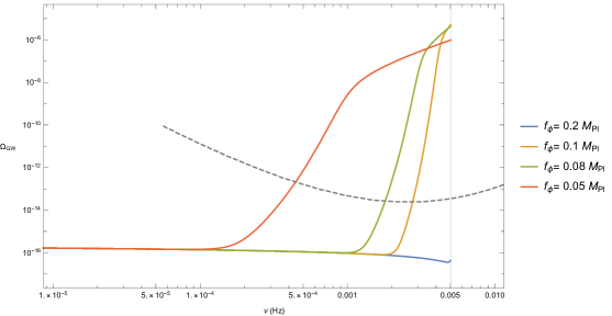
Figure 4: Abundance of gravitational waves as a function of frequency, setting $N_{\rm CMB}=35$. The dashed grey line is the sensitivity of LISA, while the horizontal thin line is the bound from the number of relativistic degrees of freedom coming from BBN and CMB. Again, we use $M_{1}^{4}=2\times 10^{-9}M_{\mathrm{Pl}}$, $\mu_{1}=M_{\mathrm{Pl}}$, $p=2/5$ for convenience, and as before scan $f_{\phi}$ as shown in the legend. The vertical line again designates the end of inflation, beyond which a different approximation is needed.

Here our main interest are the stochastic gravity waves produced near the end of the first stage of inflation. These modes are chiral, and their abundance can be estimated by [43]

$$\Omega_{GW}\equiv\frac{\Omega_{r,0}}{24}\Delta_{T}^{2}\simeq\frac{\Omega_{r,0}}{12}\left(\frac{H}{\pi M_{\mathrm{Pl}}}\right)^{2}\left(1+4.3\cdot 10^{-7}\frac{H^{2}}{M_{\mathrm{Pl}}^{2}\xi^{6}}e^{4\pi\xi}\right)\,,$$ (9)

where $\Omega_{r,0}=8.6\cdot 10^{-5}$ is the radiation abundance today, and the terms are evaluated at horizon crossing. The term in parenthesis adds to the standard tensors produced by metric fluctuations in de Sitter space the “secondary” production by the $U(1)$ vector gauge field. Its contribution tops the metric fluctuations near the end of the first stage of inflation.

Note, some of the modes produced just before the end of stage 1 would reenter the horizon during the intermediate matter-dominated stage. As a result, they would dilute by expansion during that epoch. Thus the formula for the abundance (9) should include an extra suppression factor. To estimate it, note that for subhorizon modes, the amplitude dilutes as $1/\lambda\sim 1/a$, where $a$ is the scale factor. The power in the modes is given by the square of the product of the frequency and the amplitude, since these modes behave as harmonic oscillators. Hence the suppression factor will be at most $(a_{1}/a_{2})^{4}$ where $a_{1}$ is the scale factor at the end of stage 1 of inflation, and $a_{2}$ the scale factor at the mode re-freezing after the beginning of the stage 2 of inflation. This factor is maximized for the shortest wavelength mode at the end of stage 1, for which $k/a_{1}\sim H_{1}$. Since the mode freeze-out gives $k/a_{2}\simeq H_{2}$, this yields $a_{1}/a_{2}~{}\mbox{\raisebox{-2.58334pt}{$\stackrel{{\scriptstyle<}}{{\sim}}$}}~{}H_{2}/H_{1}$. For a short intermediate stage this would suppress the power by at most a factor of 100 to 1000. This suppression would only be a subleading effect, which we ignored here. A more precise calculation of these effects would be in order, however, since this extra suppression actually helps to evade any conflicts with the BBN bound on gravity waves depicted in Fig. (4).

To get an idea how large these modes are, and at which scales they occur, we express $\Omega_{GW}$ as a function of the frequency observed in instruments at the present time. Since the comoving frequency is $\nu=k/(2\pi)$, we obtain the expression for the frequency in terms of the number of efolds before the end of inflation:

$$N=N_{CMB}+\ln\frac{k_{\rm CMB}}{0.002\textrm{Mpc}^{-1}}-44.9-\ln\frac{\nu}{10^{2}\textrm{Hz}}\,,$$ (10)

where $k_{CMB}=0.002\textrm{Mpc}^{-1}$ is the CMB pivot scale, and $N_{\rm CMB}$ is the number of efolds before the end of the first stage of inflation where the CMB scales froze out. We then re-plot the results of Fig. 3 in terms of the new independent variable $\nu$. The results are presented in Fig. 4. Again the approximations which we employ are unreliable beyond the end of inflation, where we terminate the plots. Beyond it the curves would bend down. Nevertheless it is clear that these modes are out there for LISA to see. Combined with the bounds on $r$ at the CMB scales, which are within reach of the future CMB polarization instruments, this makes our double-coaster extremely predictive and easy to falsify – or perhaps, confirm. Interestingly, not only would this be a search for a specific inflationary model, but also a quest for traces of naturalness on the sky.

4 Summary

To summarize, we have described a very predictive theory of axion monodromy inflation. The main difference from the usual realizations of monodromy inflation is that inflation is not smooth, but happens in bursts as in rollercoaster cosmology. The example we focused on involves two axions which feature a little hierarchy between their masses, with initial conditions similar to Nflation. We motivate the models by combining bounded field ranges with naturalness.

Due to a little mass hierarchy, however, the axions fall out of slow roll at different times, leading to two stages of monodromy inflation separated by a stage of matter domination, during which the first inflaton oscillates briefly before the second inflaton takes over. Clearly these masses need to be tuned, although the required tuning does not need to be exceedingly precise. If the field ranges are ${\cal O}(M_{Pl})$, and axion potentials are flattened due to being close to the cutoff and in strong coupling regime, it is straightforward to arrange for the two stages of inflation to last ${\cal N}\sim 30-40$ and ${\cal N}\sim 20-30$ efolds, respectively.

This yields the scalar and tensor perturbations at the largest scales which fit the CMB perfectly, with $0.02~{}\mbox{\raisebox{-2.58334pt}{$\stackrel{{\scriptstyle<}}{{\sim}}$}}~{}r~{}\mbox{\raisebox{-2.58334pt}{$\stackrel{{\scriptstyle<}}{{\sim}}$}}~{}0.06$, in the range of LiteBIRD and CMB-S4 experiments. In addition when the first inflaton couples to a hidden sector $U(1)$, which is quite generic in flux monodromy models where axions arise from dimensional reduction of higher rank $p$-forms, there will be an enhanced production of vectors near the end of the first stage of inflation. These modes source tensors during the short epoch of matter domination. These tensors are chiral, with wavelengths at the present time in the range of $10^{8}$ km, and with amplitudes enhanced over the long wavelength modes by vector sources. They are a very loud signal for LISA. Hence we find that double monodromy inflation easily yields simultaneous signals accessible to future gravity wave instruments at different scales.

Acknowledgments: We would like to thank A. Lawrence, E. Silverstein, L. Sorbo and especially V. Domcke for useful discussions. NK is supported in part by the DOE Grant DE-SC0009999. AW is supported by the ERC Consolidator Grant STRINGFLATION under the HORIZON 2020 grant agreement no. 647995.

References

- [1] A. H. Guth, “The Inflationary Universe: A Possible Solution to the Horizon and Flatness Problems,” Adv. Ser. Astrophys. Cosmol. 3 (1987) 139–148.
- [2] A. D. Linde, “A New Inflationary Universe Scenario: A Possible Solution of the Horizon, Flatness, Homogeneity, Isotropy and Primordial Monopole Problems,” Adv. Ser. Astrophys. Cosmol. 3 (1987) 149–153.
- [3] A. Albrecht and P. J. Steinhardt, “Cosmology for Grand Unified Theories with Radiatively Induced Symmetry Breaking,” Adv. Ser. Astrophys. Cosmol. 3 (1987) 158–161.
- [4] C. Collins and S. Hawking, “Why is the Universe isotropic?,” Astrophys. J. 180 (1973) 317–334.
- [5] N. Kaloper, A. Lawrence, and L. Sorbo, “An Ignoble Approach to Large Field Inflation,” JCAP 1103 (2011) 023, arXiv:1101.0026 [hep-th].
- [6] E. Silverstein and A. Westphal, “Monodromy in the CMB: Gravity Waves and String Inflation,” Phys. Rev. D78 (2008) 106003, arXiv:0803.3085 [hep-th].
- [7] L. McAllister, E. Silverstein, and A. Westphal, “Gravity Waves and Linear Inflation from Axion Monodromy,” Phys.Rev. D82 (2010) 046003, arXiv:0808.0706 [hep-th].
- [8] N. Kaloper and L. Sorbo, “A Natural Framework for Chaotic Inflation,” Phys. Rev. Lett. 102 (2009) 121301, arXiv:0811.1989 [hep-th].
- [9] X. Dong, B. Horn, E. Silverstein, and A. Westphal, “Simple exercises to flatten your potential,” Phys.Rev. D84 (2011) 026011, arXiv:1011.4521 [hep-th].
- [10] N. Kaloper and A. Lawrence, “Natural chaotic inflation and ultraviolet sensitivity,” Phys. Rev. D90 no. 2, (2014) 023506, arXiv:1404.2912 [hep-th].
- [11] L. McAllister, E. Silverstein, A. Westphal, and T. Wrase, “The Powers of Monodromy,” JHEP 09 (2014) 123, arXiv:1405.3652 [hep-th].
- [12] G. D’Amico, N. Kaloper, and A. Lawrence, “Monodromy Inflation in the Strong Coupling Regime of the Effective Field Theory,” Phys. Rev. Lett. 121 no. 9, (2018) 091301, arXiv:1709.07014 [hep-th].
- [13] G. D’Amico and N. Kaloper, “Rollercoaster Cosmology,” arXiv:2011.09489 [hep-th].
- [14] M. Cicoli, S. Downes, B. Dutta, F. G. Pedro, and A. Westphal, “Just enough inflation: power spectrum modifications at large scales,” JCAP 12 (2014) 030, arXiv:1407.1048 [hep-th].
- [15] M. Braglia, D. K. Hazra, F. Finelli, G. F. Smoot, L. Sriramkumar, and A. A. Starobinsky, “Generating PBHs and small-scale GWs in two-field models of inflation,” JCAP 08 (2020) 001, arXiv:2005.02895 [astro-ph.CO].
- [16] G. Tasinato, “An analytic approach to non-slow-roll inflation,” arXiv:2012.02518 [hep-th].
- [17] J. Fumagalli, S. Renaux-Petel, and L. T. Witkowski, “Oscillations in the stochastic gravitational wave background from sharp features and particle production during inflation,” arXiv:2012.02761 [astro-ph.CO].
- [18] L. Anguelova, “On Primordial Black Holes from Rapid Turns in Two-field Models,” arXiv:2012.03705 [hep-th].
- [19] M. Braglia, X. Chen, and D. K. Hazra, “Probing Primordial Features with the Stochastic Gravitational Wave Background,” JCAP 03 (2021) 005, arXiv:2012.05821 [astro-ph.CO].
- [20] C. Gordon, D. Wands, B. A. Bassett, and R. Maartens, “Adiabatic and entropy perturbations from inflation,” Phys. Rev. D 63 (2000) 023506, arXiv:astro-ph/0009131.
- [21] Y. M. Welling, Spectroscopy of Two-Field Inflation. PhD thesis, Leiden U., 11, 2018.
- [22] B. A. Campbell, N. Kaloper, R. Madden, and K. A. Olive, “Physical properties of four-dimensional superstring gravity black hole solutions,” Nucl. Phys. B 399 (1993) 137–168, arXiv:hep-th/9301129.
- [23] J. L. Cook and L. Sorbo, “Particle production during inflation and gravitational waves detectable by ground-based interferometers,” Phys. Rev. D 85 (2012) 023534, arXiv:1109.0022 [astro-ph.CO]. [Erratum: Phys.Rev.D 86, 069901 (2012)].
- [24] L. Senatore, E. Silverstein, and M. Zaldarriaga, “New Sources of Gravitational Waves during Inflation,” JCAP 08 (2014) 016, arXiv:1109.0542 [hep-th].
- [25] D. Polarski and A. A. Starobinsky, “Spectra of perturbations produced by double inflation with an intermediate matter dominated stage,” Nucl. Phys. B 385 (1992) 623–650.
- [26] S. Pi, M. Sasaki, and Y.-l. Zhang, “Primordial Tensor Perturbation in Double Inflationary Scenario with a Break,” JCAP 06 (2019) 049, arXiv:1904.06304 [gr-qc].
- [27] T. Banks, M. Dine, P. J. Fox, and E. Gorbatov, “On the possibility of large axion decay constants,” JCAP 06 (2003) 001, arXiv:hep-th/0303252.
- [28] P. Svrcek and E. Witten, “Axions In String Theory,” JHEP 06 (2006) 051, arXiv:hep-th/0605206.
- [29] M. Dias, J. Frazer, and A. Westphal, “Inflation as an Information Bottleneck - A strategy for identifying universality classes and making robust predictions,” JHEP 05 (2019) 065, arXiv:1810.05199 [hep-th].
- [30] S. Dimopoulos, S. Kachru, J. McGreevy, and J. G. Wacker, “N-flation,” JCAP 08 (2008) 003, arXiv:hep-th/0507205.
- [31] BICEP2, Keck Array Collaboration, P. Ade et al., “BICEP2 / Keck Array x: Constraints on Primordial Gravitational Waves using Planck, WMAP, and New BICEP2/Keck Observations through the 2015 Season,” Phys. Rev. Lett. 121 (2018) 221301, arXiv:1810.05216 [astro-ph.CO].
- [32] CMB-S4 Collaboration, K. N. Abazajian et al., “CMB-S4 Science Book, First Edition,” arXiv:1610.02743 [astro-ph.CO].
- [33] N. Arkani-Hamed, L. Motl, A. Nicolis, and C. Vafa, “The string landscape, black holes and gravity as the weakest force,” JHEP 06 (2007) 060, arXiv:hep-th/0601001.
- [34] H. Ooguri and C. Vafa, “On the Geometry of the String Landscape and the Swampland,” Nucl. Phys. B766 (2007) 21–33, arXiv:hep-th/0605264 [hep-th].
- [35] A. Hebecker, F. Rompineve, and A. Westphal, “Axion Monodromy and the Weak Gravity Conjecture,” JHEP 04 (2016) 157, arXiv:1512.03768 [hep-th].
- [36] N. Kaloper and L. Sorbo, “Where in the String Landscape is Quintessence,” Phys.Rev. D79 (2009) 043528, arXiv:0810.5346 [hep-th].
- [37] E. Witten, “String theory dynamics in various dimensions,” Nucl. Phys. B 443 (1995) 85–126, arXiv:hep-th/9503124.
- [38] V. Domcke, V. Guidetti, Y. Welling, and A. Westphal, “Resonant backreaction in axion inflation,” JCAP 09 (2020) 009, arXiv:2002.02952 [astro-ph.CO].
- [39] M. M. Anber and L. Sorbo, “Naturally inflating on steep potentials through electromagnetic dissipation,” Phys.Rev. D81 (2010) 043534, arXiv:0908.4089 [hep-th].
- [40] A. Linde, S. Mooij, and E. Pajer, “Gauge field production in supergravity inflation: Local non-Gaussianity and primordial black holes,” Phys. Rev. D 87 no. 10, (2013) 103506, arXiv:1212.1693 [hep-th].
- [41] G. Dall’Agata, S. González-Martín, A. Papageorgiou, and M. Peloso, “Warm dark energy,” JCAP 08 (2020) 032, arXiv:1912.09950 [hep-th].
- [42] S.-L. Cheng, W. Lee, and K.-W. Ng, “Numerical study of pseudoscalar inflation with an axion-gauge field coupling,” Phys. Rev. D 93 no. 6, (2016) 063510, arXiv:1508.00251 [astro-ph.CO].
- [43] V. Domcke, F. Muia, M. Pieroni, and L. T. Witkowski, “PBH dark matter from axion inflation,” JCAP 07 (2017) 048, arXiv:1704.03464 [astro-ph.CO].
- [44] J. Garcia-Bellido, M. Peloso, and C. Unal, “Gravitational waves at interferometer scales and primordial black holes in axion inflation,” JCAP 12 (2016) 031, arXiv:1610.03763 [astro-ph.CO].
- [45] M. Peloso, L. Sorbo, and C. Unal, “Rolling axions during inflation: perturbativity and signatures,” JCAP 09 (2016) 001, arXiv:1606.00459 [astro-ph.CO].