Discovery of Interstellar trans-cyanovinylacetylene (HCCCH=CCHCN) and vinylcyanoacetylene (H₂C=CHC₃N) in GOTHAM Observations of TMC-1

Abstract

We report the discovery of two unsaturated organic species, trans-(E)-cyanovinylacetylene and vinylcyanoacetylene, using the second data release of the GOTHAM deep survey towards TMC-1 with the 100 m Green Bank Telescope. For both detections, we performed velocity stacking and matched filter analyses using Markov chain Monte Carlo simulations, and for trans-(E)-cyanovinylacetylene, three rotational lines were observed at low signal-to-noise (${\sim}$3$\sigma$). From this analysis, we derive column densities of $2\times 10^{11}$ and $3\times 10^{11}$ cm^-2 for vinylcyanoacetylene and trans-(E)-cyanovinylacetylene, respectively, and an upper limit of $<2\times 10^{11}$ cm^-2 for trans-(Z)-cyanovinylacetylene. Comparisons with G3//B3LYP semi-empirical thermochemical calculations indicate abundances of the [H3C5N] isomers are not consistent with their thermodynamic stability, and instead their abundances are mainly driven by dynamics. We provide discussion into how these species may be formed in TMC-1, with reference to related species like vinyl cyanide (CH2=CHC#N). As part of this discussion, we performed the same analysis for ethyl cyanide (CH3CH2C#N), the hydrogenation product of CH2=CHC#N. This analysis provides evidence—at 4.17$\sigma$ significance—an upper limit to the column density of $<4\times 10^{11}$ cm^-2; an order of magnitude lower than previous upper limits towards this source.

1 Introduction

Radio observations of the Taurus Molecular Cloud (TMC) complex, particularly towards the prestellar cloud core TMC-1, have revealed a plethora of molecules ranging from the cyanopolyynes (HC_nN, for odd values of $n$), to free radicals [e.g., l-C3H by Thaddeus et al. (1985)], to carbenes (e.g. H2C6 by Langer et al. (1997)), to ions (e.g., C8H- by Brünken et al. (2007)). More recently, the discovery of benzonitrile (c-C6H5CN) by McGuire et al. (2018) adds an aromatic ring— noteworthy for its exceptional thermodynamic and chemical stability, and a key building block in biological systems and the formation of soot and interstellar dust—to this already rich inventory. Chemical models, however, currently do not have a sufficiently efficient pathway to reproduce the abundance of these aromatic molecules, in part due to the lack of observational constraints on potential carbon-chain precursors (Burkhardt et al., 2020). Unlike the well-studied cyanopolyyne family, many of the partially saturated carbon-chains have never been detected and thus large unknowns for these models. As such, in order to determine the formation of even the simplest aromatics, robust abundance measurements of partially saturated must be obtained. Understanding how molecules like benzonitrile may be formed, processed, and transported in the interstellar medium—in particular in cold, dark environments like TMC-1—has significant implications in the chemical evolution of these environments.

Our large-scale observing campaign with the 100 m Green Bank Telescope, GOTHAM (GBT Observations of TMC-1: Hunting for Aromatic Molecules), seeks to determine the chemical inventory of TMC-1 at an unprecedented level by performing a wide band spectral line survey at centimeter wavelengths at high uniform sensitivity (target 2 mK RMS across the whole spectrum) and high resolution (0.05 km s^-1). As part of the first data release, molecules of considerable complexity were reported for the first time, including 1- and 2-cyanonaphthalene (C10H7CN) (McGuire et al., 2020a), c-C5H5CN (McCarthy et al., 2020b), HC11N (Loomis et al., 2020), and HC4NC (Xue et al., 2020). Many of these detections greatly benefited from combining signal processing techniques with Bayesian modeling, which enables identification of molecules in sparse line spectra even when no individual features are present above the noise. Furthermore, statistically robust derivations of parameters such as column density and excitation temperature can be determined using this treatment. For an overview of this method and its use cases, the reader is referred to McGuire et al. (2020b).

In this paper, we examine evidence in the second data release of GOTHAM for three isomers in the H3C5N family: vinylcyanoacetylene (H2C=CHC3N, VCA), and the ($E$) and ($Z$) isomers of trans-cyanovinylacetylene (HC#CCH=CHC#N, CVA), as shown in Fig. 1. They are extended variants of vinyl cyanide (CH2CHCN), an unsaturated nitrile-bearing molecule which was first detected in this source by Matthews & Sears (1983). Given questions still persist as to how small branched hydrocarbon chains form in TMC-1 despite their structural simplicity (Vigren et al., 2009), simultaneous analysis of multiple isomers may provide insight into the operative formation pathways there. Of particular interest for this isomeric family is the possible connection with aromatic N-heterocycles such as pyridine, $c$-C5H5N, which might be formed by subsequent hydrogenation of one or more of the these isomers followed by ring closure.

2 Observations

Observations with the 100 m Green Bank Telescope (GBT) were carried out for the GOTHAM project, which has been detailed in a series of publications. Briefly, this work uses the second data release (henceforth referred to as DR2) of GOTHAM, which are observations targeting the well-known TMC-1 cyanopolyyne peak (CP) centered at $\alpha_{\mathrm{J2000}}$ = 04$\fh$41$\fm$42.5$\fs$, $\delta$ = +25°41′26.8″(McGuire et al., 2020b). As of DR2, our spectra cover the GBT X-, K-, and Ka-bands from 7.906 to 33.527 GHz (25.6 GHz bandwidth) with continuous coverage between 22–33.5 GHz, at a uniform frequency resolution of 1.4 kHz (0.05–0.01 km/s in velocity) and an RMS noise of ${\sim}2$–20 mK across the spectrum, with the RMS increasing towards higher frequency due to limited integration time. Uncertainty due to flux calibration is expected to be $\sim$20%, based on complementary VLA observations of the flux-calibrator source J0530+1331 (McGuire et al., 2020b).

3 Computational methods

3.1 Quantum chemistry

Calculations of the permanent electric dipole moment and relative energetics were performed using the Gaussian fl16 suite of electronic structure programs (Frisch et al., 2016). For dipole moments, geometries were first optimized at the $\omega$B97X-D/6-31+G(d) level of theory, and the one-electron properties calculated at the same level—based on our earlier benchmarking, this combination produces dipole moments with uncertainties on the order of $\pm 0.5$ D and systematically over-predicts vibrationally averaged values by 0.1 D (Lee & McCarthy, 2020). In terms of thermochemistry, we used the B3LYP variant of the G3 semi-empirical model chemistry (Baboul et al., 1999), which has been shown to be a computationally cost-effective method of obtaining near-chemically accurate energetics (${\sim}$120 K) (Simmie & Somers, 2015).

3.2 MCMC modeling

Details of the Markov chain Monte Carlo (MCMC) simulations are described in depth by Loomis et al. (2020), and we only briefly discuss the relevant aspects here. The objective of these simulations is to properly model the physical parameters of molecules in TMC-1 where maximum likelihood methods generally fail due to high covariance and dimensionality. The model used in our study assumes a Gaussian shape for the spatial distribution of TMC-1, with parameters for the size of the source ($SS$), radial velocity ($v_{\mathrm{LSRK}}$), column density ($N_{\mathrm{col}}$), excitation temperature ($T_{\mathrm{ex}}$), and spectral linewidth ($dv$). Based on recent observations performed with the 45 m telescope at Nobeyama Radio Observatory (Dobashi et al., 2018, 2019; Soma et al., 2018), as well as our data (Loomis et al., 2020), emission from molecules in TMC-1 towards the cyanopolyyne peak display at least four individual velocity components which are subsequently represented by independent source size, radial velocity, and column density parameters; in total, our model comprises 14 fitting parameters.

Line profile simulations were performed using molsim (Lee & McGuire, 2020). The MCMC simulations used wrapper functions in molsim to arviz (Kumar et al., 2019) and emcee (Foreman-Mackey et al., 2013); the former for analyzing the results of sampling, and the latter implements an affine-invariant MCMC sampler. As a prior parameters, we used the marginalized posterior from modeling HC9N chosen based on chemical similarity. The prior distributions approximated as normal (i.e. $p(\theta)\sim N(\mu_{\theta},\sigma_{\theta})$ for parameter $\theta$) with modifications to the variance $\sigma_{\theta}$ as to avoid overly constrictive/influential priors. The MCMC analysis was performed first for trans-(E)-CVA, which produced the strongest response out of the molecules reported here. Convergence of the MCMC was confirmed using standard diagnostics such as the Gelman & Rubin (1992) $\hat{R}$ statistic, and by visually inspecting the posterior traces. The resulting posterior for trans-(E)-CVA was subsequently used as prior distributions for VCA and trans-(Z)-CVA, albeit with the source sizes constrained to the mean values of trans-(E)-CVA due to poorly convergent sampling. The results reported here are relatively insensitive to the choice of prior; comparison between benzonitrile and trans-(E)-CVA do not qualitatively change the statistics derived from the converged posteriors.

3.3 Velocity stacking and matched filter analysis

With the model posterior at hand, we can corroborate our simulations with the observed data through a combined velocity stack and matched filter analysis (Loomis et al., 2018, 2020). Briefly, the former involves a noise-weighted composite spectrum by stacking the observed spectra—in velocity space—using known molecular transition frequencies, and the latter performs a velocity stack of the spectral simulation based on the fitted parameters, and cross-correlated with the observational velocity stack. The advantage of this approach is the ability to derive statistical significance of a detection based on the impulse response in the cross-correlation: the significance, $\sigma$, directly quantifies how well our model reproduces the observed data in velocity space, even in lieu of individual observed transitions. Throughout the GOTHAM studies, we have adopted a $\geq$5$\sigma$ heuristic for what constitutes a molecular detection as determined by HC11N (Loomis et al., 2020).

4 Results & discussion

4.1 Spectroscopy & relative energetics

Figure 1 shows the relative energetics of the four molecules under investigation, along with their equilibrium structures. The two lowest energy forms of [H3C5N] are near-prolate tops, while the two higher energy forms are closer to the oblate limit. The highest energy form in our study, cis-cyanovinylacetylene, has not yet been experimentally observed whereas the remaining three isomers have been studied extensively in the laboratory (Halter et al., 2001; Thorwirth et al., 2004), and most recently observed in a discharge mixture of benzene and N2 (McCarthy et al., 2020a). We have also omitted the linear chain form, CH3C4N, which is likely to be unstable by analogy to the cyanpolyynes.

Catalogs of rotational transitions were generated using the SPCAT program (Pickett, 1991) based on spectroscopic parameters—including nitrogen-hyperfine splitting—reported in the cited publications. In all cases, our electronic structure calculations suggest sizable dipole moments along $a$ and $b$-inertial axes (Table 1) with the total dipole moment around ${\sim}5$ D; typical for -C#N bearing molecules. For the two molecules closer to the oblate limit, the total dipole moment is divided roughly equally between the $a$ and $b$-axes. Given that $I\propto\mu^{2}$, this means that on an individual line basis, the near-oblate isomers require an order of 2–3 times more sensitivity for detection compared to their near-prolate counterparts.

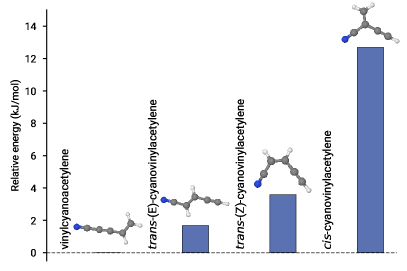
Figure 1: G3//B3LYP energetics of the [H3C5N] structures of interest at 0 K, given relative to the lowest energy form vinylcyanoacetylene.

Table 1: Theoretical equilibrium dipole moments for the molecules of interest. Values are calculated at the $\omega$B97X-D/6-31+G(d) level of theory, which have a nominal $\pm$0.5 D uncertainty (see Section 3.1).

	$\mu_{a}$	$\mu_{b}$
	(Debye)	(Debye)
VCA	5.3	0.3
trans-(E)-CVA	4.2	0.6
trans-(Z)-CVA	2.7	2.8
cis-CVA	3.2	2.5

4.2 GOTHAM observations

Based on the energetics shown in Figure 1, we attempted to search for individual transitions arising from the lower energy isomers. Upon inspection, the lowest energy isomer, VCA, does not exhibit any obvious features in our spectra. For the next isomer in energy, trans-$(E)$-CVA, Figure 2 shows three spectral windows centered at frequencies that correspond to two $K=0$ and one $K=1$ transitions. These windows hint at individual spectral features within our data, albeit at low significance.

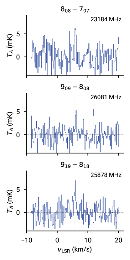
Figure 2: Observed spectral features in the GOTHAM spectrum (rebinned to 14 kHz resolution) at the center frequencies for three a-type transitions of trans-(E)-CVA. The dashed vertical line indicates the nominal source velocity at 5.8 km/s. Asymmetric top ($J_{K_{a}K_{c}}$) quantum number assignments are given at the top of each trace, along with their rest frequencies. The peak signal-to-noise ratio for each spectrum is on the order of ${\sim}$3$\sigma$.

4.3 Velocity stack and matched filter analysis

From our observations, only trans-(E)-CVA exhibits tentative individual spectral features—whereas conventional methods of analysis (i.e. least-squares fits) may be limited to deriving upper limits to column densities, here we can combine velocity stacking and matched filter analysis with MCMC simulations to derive statistically robust molecular parameters for all three isomers. Figure 3 visualizes the detection of VCA and trans-(E)-CVA, and non-detection of trans-(Z)-CVA with the velocity stack and matched filter analyses.

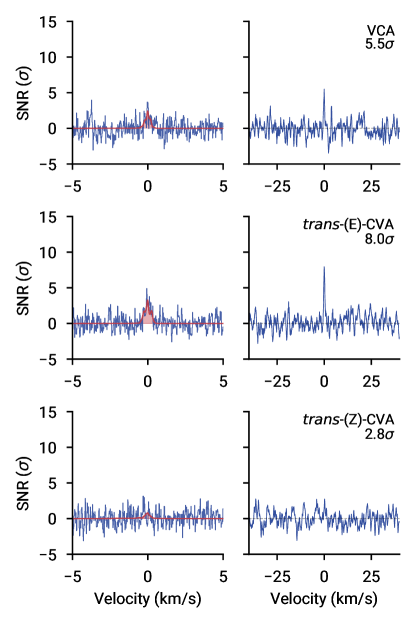
Figure 3: Velocity stack (left columns) and corresponding matched filter (right columns) for the three molecules of interest. Peak impulse responses—shown in units of signal-to-noise (SNR)—are provided in the matched filter plots. The velocity stack of simulated spectra using parameters derived from the MCMC simulations are overlaid in red.

The velocity stacks in Figure 3 indicate the presence of additive spectral intensity across the GOTHAM survey for VCA and trans-(E)-CVA, and none for trans-(Z)-CVA. For each stack, the red traces show the velocity stack for simulated spectra based on the posterior means from the MCMC simulations, which in all cases agrees well with the stacks based on observations. The two velocity stacks corroborate in the matched filter, simultaneously visualizing the overlap between model and observations, and providing an estimate of the significance of our detection. For VCA and trans-(E)-CVA, the matched filters exhibit a response clearly above the noise, whereas for trans-(Z)-CVA this is not the case and thus we report only an upper limit to the column density for this molecule. Table 2 summarizes the derived column densities and excitation temperatures from the MCMC simulations.

Table 2: Total column densities and excitation temperatures derived from the MCMC simulations. Uncertainties are given as the 95% credible interval. Unabridged MCMC results can be found in the Appendix. Interlopers refer to interfering features of other species, detected as $3\sigma$ for a given spectral chunk.

Molecule	Column density	$T_{\mathrm{ex}}$
	(1011 cm-2)	(K)
VCA	1.87${}^{+0.37}_{-0.38}$	6.7${}^{+0.6}_{-0.6}$
trans-(E)-CVA	2.90${}^{+0.41}_{-0.40}$	7.0${}^{+1.2}_{-1.3}$
trans-(Z)-CVA	$<2$	—

4.4 Astrochemical implications

Based on our systematic investigation of the three lowest energy isomers of [H3C5N], we can infer some details into the relative importance of dynamical pathways that lead to the overall chemical inventory of TMC-1—particularly the branched unsaturated hydrocarbons we see here. In all cases, the excitation temperatures we estimate are on the order of ${\sim}7$ K—consistent with those reported for other molecules in TMC-1 (Dobashi et al., 2018, 2019). The velocity profiles are also similar between each isomer, allowing us to assume that they are cospatial within each velocity component. Of the two isomers we successfully detected, VCA is approximately two times less abundant than trans-(E)-CVA, despite being more thermodynamically stable (${\sim}$240 K), thus their relative abundance is dominated by dynamics. The third isomer, trans-(Z)-CVA, does not exhibit a significant response in either the velocity stack nor the matched filter (Figure 3). However, our MCMC simulations indicate that it may be just below our current sensitivity limits (see Appendix A2).

Given that the relative abundances are likely dictated by kinetics, the question now turns to how the three isomers may be preferentially formed in TMC-1. In the gas-phase, neutral-neutral reactions are an attractive route: radicals such as C2H and CN can react with CH2=CHC#N (vinyl cyanide) and CH2=CHC#CH (vinyl acetylene), followed by hydrogen loss. The reaction C2H + CH2=CHC#N and would produce stereoisomers of CVA, with a preference for the trans isomers due to steric hinderance owing to the acetylenic unit. While this specific reaction has not yet been studied experimentally, by analogy to similar reactions between C2H and unsaturated hydrocarbons [C2H2 (Kovács et al., 2010; Chastaing et al., 1998; Zhang et al., 2009)]; C2H4, C3H6 (Bouwman et al., 2012; Krishtal et al., 2009; Chastaing et al., 1998)] we expect this reaction to be barrierless and efficient even at low temperatures. The latter reaction, CN + CH2=CHC#CH, can form all three [H3C5N] isomers considered in Figure 1; experimental studies by Yang et al. (1992); Sims et al. (1993) suggests CN addition is just as efficient to either the vinyl (forming CVA) or acetylenic unit (forming VCA) (Balucani et al., 2000; Choi et al., 2004) . Additionally, VCA can be formed through the reaction between C3N + C2H4 involving submerged barriers (Moon & Kim, 2017); experimental kinetic data for this reaction is not yet available to the best of our knowledge.

Alternatively, grain surface reactions are a well-established pathway to hydrogenate unsaturated species efficiently (Herbst, 2001; Cuppen et al., 2017). In this context, [H3C5N] molecules would be formed through HC5N + H2 hydrogenation, with the isomeric ratio dependent on the relative cross-section or likelihood of attaching H2 to each respective part of the chain, which in turn is dictated by whether this occurs in a concerted (+H2) or stepwise (+ H + H) fashion. The former is likely to be highly endothermic and therefore unlikely under cold, dark conditions, while the latter is facilitated by hydrogen atom tunneling. A similar route had been proposed for CH2CHCN, with HC3N as the precursor (Blake et al., 1987). Analysis by Loomis et al. (2020) suggests HC5N is approximately an order of magnitude less abundant than HC3N, which corresponds well with isomers of the [H3C5N] family and CH2CHCN, where the column density of the latter was determined by Matthews & Sears (1983) to be on the order of 3$\times 10^{12}$ cm^-2. An argument against hydrogenation reactions, however, is that prior to sublimation from the grain they should ultimately form saturated species that are known to be uncommon in TMC-1: for instance, ethyl cyanide (CH3CH2CN) should form from hydrogenation of CH2CHCN (Blake et al., 1987). Minh & Irvine (1991) were only able to place upper limits on CH3CH2CN; using the same velocity stack and matched filter methodology, we tentatively ascribe an upper limit to the total column density of $<4\times 10^{11}$ cm^-2 (given as the 97.5th percentile; see Appendix A.4), consistent with their determination ($<3\times 10^{12}$ cm^-2).

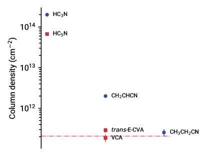
Figure 4: Column densities for assumed co-spatial HC3N and HC5N (Loomis et al., 2020), CH2CHCN (Matthews & Sears, 1983), CH3CH2CN (Appendix A.4), and the newly detected molecules toward TMC-1. The error bars represent 1$\sigma$ uncertainty.

While it is difficult to draw conclusions with confidence at this level of significance, it appears that the decrement in column density follows a qualitative trend (Figure 4) that lends credit to sequential hydrogenation (HC3N -¿[+H2] CH2CHCN -¿[+H2] CH3CH2CN). Better constraints on CH3CH2CN, as well as the missing isomer trans-(Z)-CVA will provide critical insight into the relative importance of gas phase and grain hydrogenation pathways.

If the hydrogenation route is indeed a large contributing mechanism, then VCA and trans-(E)-CVA would be important intermediates toward the formation of cyclic molecules—specifically the still-elusive N-heterocycles such as pyrrole and pyridine, and the recently detected 1-cyanocyclopentadiene. In the former, we note that trans-(Z)-CVA is a hydrogenation (+H2) and ring closing step from pyridine—a molecule of biological importance. Further study into this isomeric family, particularly cis-CVA and the deuterated isotopologues (similar to previous work on cyanopolyyne isotopologues by Burkhardt et al. (2018)), should reveal the dynamical processes behind the formation of these molecules, although their laboratory spectra have not yet been measured.

5 Conclusions

From our GOTHAM observations, we report the first detection of two new isomers of [H3C5N] toward TMC-1, and more generally in the interstellar medium. Combining MCMC simulations with velocity stacking and matched filter analysis, we were able to successfully characterize vinylcyanoacetylene (VCA) and trans-(E)-cyanovinylacetylene (CVA) at 5.5$\sigma$ and 8.0$\sigma$ significance respectively, with derived column densities on the order of $1\times 10^{11}$ and $2\times 10^{11}$ cm^-2 respectively. The third isomer, trans-(Z)-CVA, appears to be just out of reach at current integration levels, and from our MCMC analysis we place an upper limit for its column density at $<2\times 10^{11}$ cm^-2. While it remains unclear how these unsaturated hydrocarbons may be formed in TMC-1, we discuss implications of cyanopolyyne hydrogenation on grain surfaces—as part of this analysis, we also report a tentative detection of ethyl cyanide with a MCMC derived upper limit to the total column density of $<4\times 10^{11}$ cm^-2. Further analysis into the [H3C5N] family, and other related hydrocarbon chains will help reveal the complex formation processes taking place, and more broadly, how molecules more saturated than cyanopolyynes could be formed under cold, dark conditions.

6 Data access & code

Data used for the MCMC analysis can be found in the DataVerse entry (GOTHAM, 2020). The code used to perform the analysis is part of the molsim open-source package; an archival version of the code can be accessed at Lee & McGuire (2020).

Appendix A MCMC posterior analysis

A.1 trans-(E)-CVA

Figure A1 shows the results of the MCMC fit for trans-(E)-CVA. There are several factors that warrant extra discussion, particularly as to how these plots can be interpreted. First, the diagonal traces correspond to the marginalized likelihood for each model parameter presented as empirical cumulative distribution function (ECDF) plots—these provide a non-parametric visualization of the likelihood, in contrast to kernel density estimates and histograms which require length scale and bin width specification respectively. Second, the off-diagonal traces correspond to kernel density plots of parameter pairs—these plots visualize the covariance between any given pair of model parameters; in our case, well-approximated by two-dimensional Gaussian distributions.

Inspection of the marginalized likelihood ECDF traces indicate firm detections in components #1, #3, and #4, with a likely non-detection in component #. In the non-detection case, the cumulative density rises linearly from zero $N_{\mathrm{col}}$, while for detections they appear clearly sigmoid-like with the inflexion point at non-zero column. Table A1 provides summary statistics for the posterior distributions.

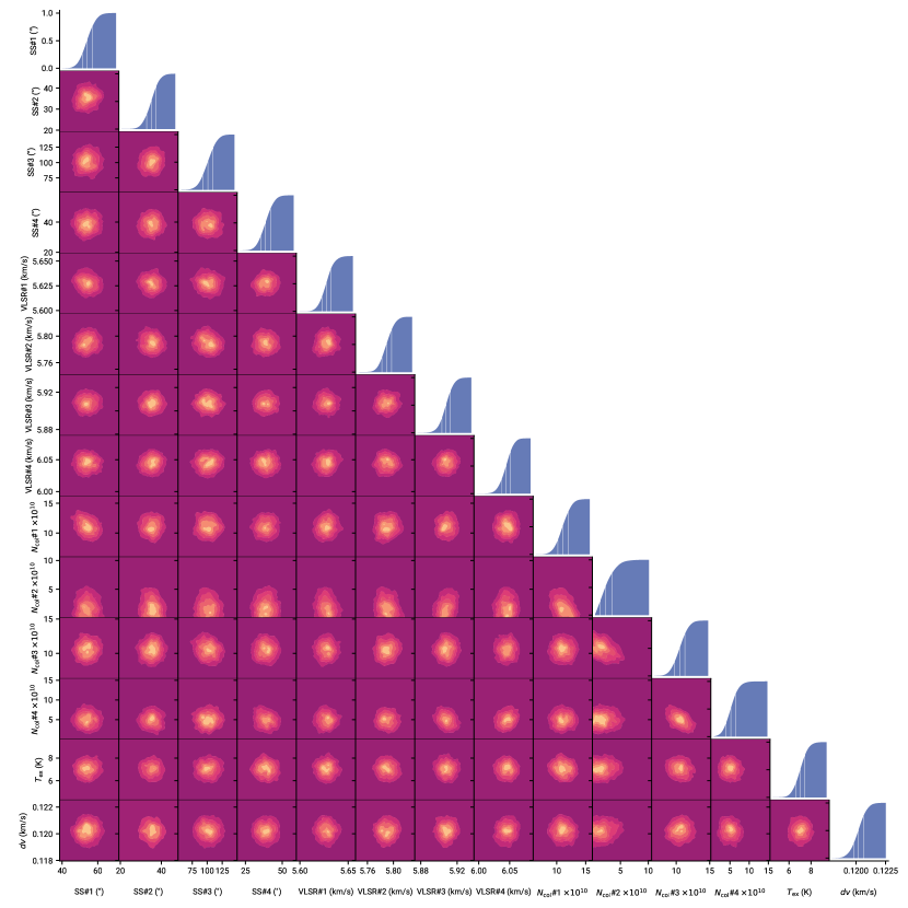
Figure A1: Corner plot for trans-(E)-CVA. The diagonal traces correspond to ECDF plots, and off-diagonal plots show the kernel density covariance between model parameters. In the former, lines represent the 25^th, 50^th, and 75^th percentiles respectively. The length scale for the kernel density plots is chosen with Scott’s rule.

Table A1: trans-(E)-CVA best-fit parameters from MCMC analysis. Quoted uncertainties correspond to the 95% highest posterior density. $N_{T}$ (Total) refers to the pooled column density from the four components, given as the posterior mean and 95% highest posterior density of the joint distributions.

Component	$v_{lsr}$	Size	$N_{\mathrm{col}}$	$T_{ex}$	$\Delta V$
	(km s-1)	(′′)	(1010 cm-2)	(K)	(km s-1)
C1	$5.628^{+0.014}_{-0.015}$	$54^{+8}_{-9}$	$11.06^{+2.51}_{-2.59}$	$7.0^{+1.2}_{-1.3}$	$0.120^{+0.001}_{-0.001}$
C2	$5.790^{+0.022}_{-0.021}$	$35^{+7}_{-7}$	$2.31^{+2.78}_{-2.31}$
C3	$5.908^{+0.015}_{-0.015}$	$101^{+26}_{-25}$	$10.52^{+2.27}_{-2.17}$
C4	$6.044^{+0.021}_{-0.021}$	$39^{+10}_{-10}$	$5.04^{+3.72}_{-3.52}$
$N_{T}$ (Total)	$28.98^{+4.13}_{-3.98}\times 10^{10}$ cm-2

A.2 trans-(Z)-CVA

Figure A2 shows the corner plot for trans-(Z)-CVA. Because these simulations fix the source size to the mean of trans-(E)-CVA, the source sizes are not sampled/fit and are omitted from the corner plot. Under these conditions, we observe most likely non-detection in component #1, with evidence for detection in the remaining three components. Given that components #2 and #3 in particular are highly indicative of trans-(Z)-CVA, we believe that this molecule is just out of reach at the current level of integration of the second GOTHAM data release. Summaries of the posterior distributions can be found in Table A2.

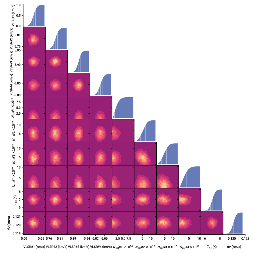
Figure A2: Corner plot for trans-(Z)-CVA. The diagonal traces correspond to ECDF plots, and off-diagonal plots show the kernel density covariance between model parameters. In the former, lines represent the 25^th, 50^th, and 75^th percentiles respectively. The length scale for the kernel density plots is chosen with Scott’s rule.

Table A2: trans-(Z)-CVA best-fit parameters from MCMC analysis. Quoted uncertainties correspond to the 95% highest posterior density. $N_{T}$ (Total) refers to the pooled column density from the four components, given as the mean and 95% highest posterior density of the joint posterior distributions.

Component	$v_{lsr}$	$N_{\mathrm{col}}$	$T_{ex}$	$\Delta V$
	(km s-1)	(1010 cm-2)	(K)	(km s-1)
C1	$5.628^{+0.017}_{-0.016}$	$1.72^{+2.45}_{-1.72}$	$7.0^{+0.7}_{-0.7}$	$0.120^{+0.001}_{-0.001}$
C2	$5.789^{+0.025}_{-0.026}$	$5.07^{+4.15}_{-4.11}$
C3	$5.910^{+0.017}_{-0.018}$	$4.47^{+3.77}_{-4.46}$
C4	$6.041^{+0.025}_{-0.025}$	$2.64^{+3.13}_{-2.64}$
$N_{T}$ (Total)	$13.96^{+6.40}_{-5.32}\times 10^{10}$ cm-2

A.3 VCA

Figure A3 visualizes the MCMC simulation results for VCA, with a similar treatment as to trans-(Z)-CVA. In contrast to the other molecules we have studied here, VCA demonstrates significant bimodality in its posterior distributions. Most of the observed flux can be explained by components #1 and #4, while our model displays large covariance with component #3, likely suggesting a three-component model where #2 and #3 are degenerate. Summaries of the posterior distributions can be found in Table A3.

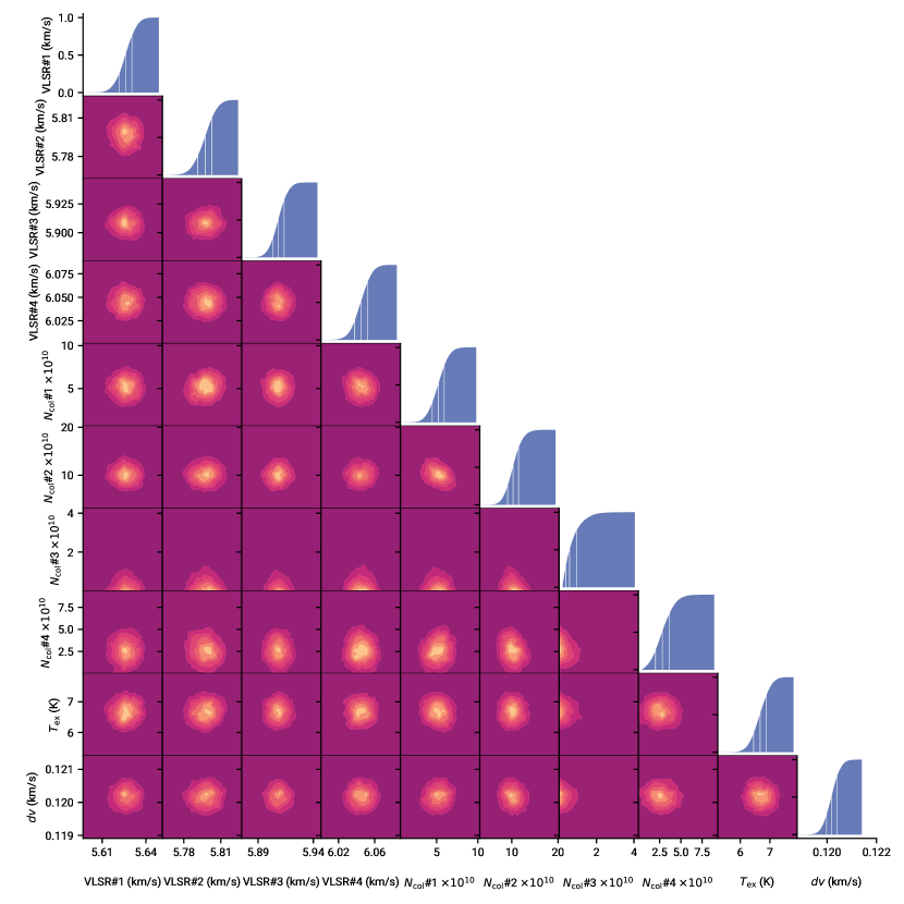
Figure A3: Corner plot for VCA. The diagonal traces correspond to ECDF plots, and off-diagonal plots show the kernel density covariance between model parameters. In the former, lines represent the 25^th, 50^th, and 75^th percentiles respectively. The length scale for the kernel density plots is chosen with Scott’s rule.

Table A3: VCA best-fit parameters from MCMC analysis. Quoted uncertainties correspond to the 95% highest posterior density. $N_{T}$ (Total) refers to the pooled column density from the four components, given as the mean and 95% highest posterior density of the joint posterior distributions.

Component	$v_{lsr}$	$N_{\mathrm{col}}$	$T_{ex}$	$\Delta V$
	(km s-1)	(1010 cm-2)	(K)	(km s-1)
C1	$5.626^{+0.013}_{-0.013}$	$5.185^{+2.183}_{-2.189}$	$6.7^{+0.6}_{-0.6}$	$0.124^{+0.003}_{-0.003}$
C2	$5.797^{+0.017}_{-0.017}$	$10.218^{+3.526}_{-3.560}$
C3	$5.908^{+0.016}_{-0.015}$	$0.569^{+1.002}_{-0.569}$
C4	$6.045^{+0.020}_{-0.021}$	$2.708^{+2.284}_{-2.474}$
$N_{T}$ (Total)	$18.669^{+3.704}_{-3.767}\times 10^{10}$ cm-2

A.4 Ethyl cyanide

As part of our analysis into the hypothesis of cyanopolyyne hydrogenation of HC5N leading to the formation of [H3C5N] isomers, we performed the same velocity stacking and matched filter analysis for ethyl cyanide, the hydrogenation product of vinyl cyanide, which in turn could be formed from hydrogenation of HC3N. The catalog for ethyl cyanide was generated using spectroscopic parameters collated in the Cologne Database for Molecular Spectroscopy (Müller et al., 2005; Endres et al., 2016).

Individual transitions of ethyl cyanide were not observed at our current level of integration. Figure A4 shows the corner plot from the MCMC simulations, indicating likely detections toward components #1 and #2, and most likely non-detections in #3 and #4—a summary of the derived parameters can be found in Table A4. At our level of integration, it appears that there is supporting evidence for a tentative detection of ethyl cyanide, albeit at relatively low significance (Figure A5): as the quality of the GOTHAM spectrum improves, we can revisit this molecule in order to place better constraints on the model parameters, and correspondingly improve the matched filter response. At its current state, we establish an upper limit to the total column density based on the 97.5th percentile value from the joint posterior of $<4\times 10^{11}$ cm^-2.

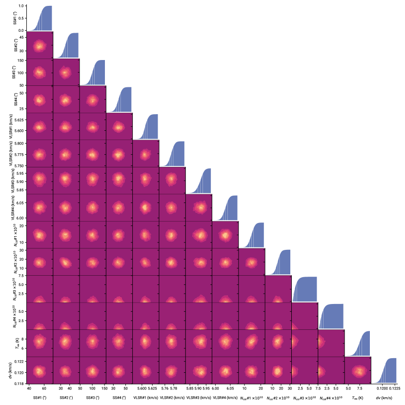
Figure A4: Corner plot for ethyl cyanide. The diagonal traces correspond to ECDF plots, and off-diagonal plots show the kernel density covariance between model parameters. In the former, lines represent the 25^th, 50^th, and 75^th percentiles respectively. The length scale for the kernel density plots is chosen with Scott’s rule.

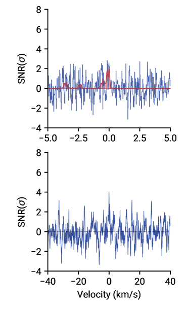
Figure A5: Velocity stack and matched filter plots for ethyl cyanide. The peak matched filter response is 4.17$\sigma$.

Table A4: Ethyl cyanide best-fit parameters from MCMC analysis. Quoted uncertainties correspond to the 95% highest posterior density. $N_{T}$ (Total) refers to the pooled column density from the four components, given as the mean and 95% highest posterior density of the joint posterior distributions.

Component	$v_{lsr}$	Size	$N_{\mathrm{col}}$	$T_{ex}$	$\Delta V$
	(km s-1)	(′′)	(1010 cm-2)	(K)	(km s-1)
C1	$5.608^{+0.014}_{-0.013}$	$54^{+9}_{-8}$	$14.29^{+3.80}_{-3.73}$	$7.4^{+1.5}_{-1.7}$	$0.120^{+0.001}_{-0.001}$
C2	$5.760^{+0.018}_{-0.018}$	$35^{+7}_{-7}$	$16.19^{+6.40}_{-6.33}$
C3	$5.914^{+0.042}_{-0.047}$	$100^{+25}_{-25}$	$0.86^{+1.38}_{-0.86}$
C4	$6.034^{+0.021}_{-0.021}$	$38^{+9}_{-10}$	$0.88^{+1.38}_{-0.88}$
$N_{T}$ (Total)	$32.05^{+4.07}_{-4.00}\times 10^{10}$ cm-2

References

- Baboul et al. (1999) Baboul, A. G., Curtiss, L. A., Redfern, P. C., & Raghavachari, K. 1999, The Journal of Chemical Physics, 110, 7650, doi: 10.1063/1.478676
- Balucani et al. (2000) Balucani, N., Asvany, O., Huang, L. C. L., et al. 2000, The Astrophysical Journal, 545, 892, doi: 10.1086/317848
- Blake et al. (1987) Blake, G. A., Sutton, E. C., Masson, C. R., & Phillips, T. G. 1987, The Astrophysical Journal, 315, 621, doi: 10.1086/165165
- Bouwman et al. (2012) Bouwman, J., Goulay, F., Leone, S. R., & Wilson, K. R. 2012, The Journal of Physical Chemistry A, 116, 3907, doi: 10.1021/jp301015b
- Brünken et al. (2007) Brünken, S., Gupta, H., Gottlieb, C. A., McCarthy, M. C., & Thaddeus, P. 2007, The Astrophysical Journal Letters, 664, L43, doi: 10.1086/520703
- Burkhardt et al. (2018) Burkhardt, A. M., Herbst, E., Kalenskii, S. V., et al. 2018, Monthly Notices of the Royal Astronomical Society, 474, 5068, doi: 10.1093/mnras/stx2972
- Burkhardt et al. (2020) Burkhardt, A. M., Loomis, R. A., Shingledecker, C. N., et al. 2020, arXiv:2009.13548 [astro-ph]. http://arxiv.org/abs/2009.13548
- Chastaing et al. (1998) Chastaing, D., James, P. L., Sims, I. R., & Smith, I. W. M. 1998, Faraday Discussions, 109, 165, doi: 10.1039/A800495A
- Choi et al. (2004) Choi, N., Blitz, M. A., McKee, K., Pilling, M. J., & Seakins, P. W. 2004, Chemical Physics Letters, 384, 68, doi: 10.1016/j.cplett.2003.11.100
- Cuppen et al. (2017) Cuppen, H. M., Walsh, C., Lamberts, T., et al. 2017, Space Science Reviews, 212, 1, doi: 10.1007/s11214-016-0319-3
- Dobashi et al. (2018) Dobashi, K., Shimoikura, T., Nakamura, F., et al. 2018, The Astrophysical Journal, 864, 82, doi: 10.3847/1538-4357/aad62f
- Dobashi et al. (2019) Dobashi, K., Shimoikura, T., Ochiai, T., et al. 2019, The Astrophysical Journal, 879, 88, doi: 10.3847/1538-4357/ab25f0
- Endres et al. (2016) Endres, C. P., Schlemmer, S., Schilke, P., Stutzki, J., & Müller, H. S. P. 2016, Journal of Molecular Spectroscopy, 327, 95, doi: 10.1016/j.jms.2016.03.005
- Foreman-Mackey et al. (2013) Foreman-Mackey, D., Hogg, D. W., Lang, D., & Goodman, J. 2013, Publications of the Astronomical Society of the Pacific, 125, 306, doi: 10.1086/670067
- Frisch et al. (2016) Frisch, M. J., Trucks, G. W., Schlegel, H. B., et al. 2016, Gaussian 16 Revision A.01
- Gelman & Rubin (1992) Gelman, A., & Rubin, D. B. 1992, in Bayesian Statistics (Oxford University Press), 625 – 631
- GOTHAM (2020) GOTHAM. 2020, Spectral Stacking Data for Phase 2 Science Release of GOTHAM, V2, Harvard Dataverse, doi: 10.7910/DVN/K9HRCK
- Halter et al. (2001) Halter, R. J., Fimmen, R. L., McMahon, R. J., et al. 2001, Journal of the American Chemical Society, 123, 12353, doi: 10.1021/ja011195t
- Herbst (2001) Herbst, E. 2001, Chemical Society Reviews, 30, 168, doi: 10.1039/A909040A
- Kovács et al. (2010) Kovács, T., Blitz, M. A., & Seakins, P. W. 2010, The Journal of Physical Chemistry A, 114, 4735, doi: 10.1021/jp908285t
- Krishtal et al. (2009) Krishtal, S. P., Mebel, A. M., & Kaiser, R. I. 2009, The Journal of Physical Chemistry A, 113, 11112, doi: 10.1021/jp904033a
- Kumar et al. (2019) Kumar, R., Carroll, C., Hartikainen, A., & Martin, O. 2019, Journal of Open Source Software, 4, 1143, doi: 10.21105/joss.01143
- Langer et al. (1997) Langer, W. D., Velusamy, T., Kuiper, T. B. H., et al. 1997, The Astrophysical Journal Letters, 480, L63, doi: 10.1086/310622
- Lee & McCarthy (2020) Lee, K. L. K., & McCarthy, M. 2020, The Journal of Physical Chemistry A, 5, 898, doi: 10.1021/acs.jpca.9b09982
- Lee & McGuire (2020) Lee, K. L. K., & McGuire, B. A. 2020, molsim, Zenodo. https://zenodo.org/record/4122749
- Loomis et al. (2020) Loomis, R. A., Burkhardt, A. M., Shingledecker, C. N., et al. 2020, arXiv:2009.11900 [astro-ph]. http://arxiv.org/abs/2009.11900
- Loomis et al. (2018) Loomis, R. A., Öberg, K. I., Andrews, S. M., et al. 2018, The Astronomical Journal, 155, 182, doi: 10.3847/1538-3881/aab604
- Matthews & Sears (1983) Matthews, H. E., & Sears, T. J. 1983, The Astrophysical Journal, 272, 149, doi: 10.1086/161271
- McCarthy et al. (2020a) McCarthy, M. C., Lee, K. L. K., Carroll, P. B., et al. 2020a, The Journal of Physical Chemistry A, 124, 5170, doi: 10.1021/acs.jpca.0c02919
- McCarthy et al. (2020b) McCarthy, M. C., Lee, K. L. K., Loomis, R. A., et al. 2020b, Nature Astronomy, 1, doi: 10.1038/s41550-020-01213-y
- McGuire et al. (2018) McGuire, B. A., Burkhardt, A. M., Kalenskii, S., et al. 2018, Science, 359, 202, doi: 10.1126/science.aao4890
- McGuire et al. (2020a) McGuire, B. A., Loomis, R. A., Burkhardt, A. M., et al. 2020a, Science
- McGuire et al. (2020b) McGuire, B. A., Burkhardt, A. M., Loomis, R. A., et al. 2020b, The Astrophysical Journal Letters, 900, L10, doi: 10.3847/2041-8213/aba632
- Minh & Irvine (1991) Minh, Y. C., & Irvine, W. M. 1991, Astrophysics and Space Science, 175, 165, doi: 10.1007/BF00644434
- Moon & Kim (2017) Moon, J., & Kim, J. 2017, Theoretical Chemistry Accounts, 136, 13, doi: 10.1007/s00214-016-2040-4
- Müller et al. (2005) Müller, H. S. P., Schlöder, F., Stutzki, J., & Winnewisser, G. 2005, Journal of Molecular Structure, 742, 215, doi: 10.1016/j.molstruc.2005.01.027
- Pickett (1991) Pickett, H. M. 1991, Journal of Molecular Spectroscopy, 148, 371, doi: 10.1016/0022-2852(91)90393-O
- Simmie & Somers (2015) Simmie, J. M., & Somers, K. P. 2015, The Journal of Physical Chemistry A, 119, 7235, doi: 10.1021/jp511403a
- Sims et al. (1993) Sims, I. R., Queffelec, J.-L., Travers, D., et al. 1993, Chemical Physics Letters, 211, 461, doi: 10.1016/0009-2614(93)87091-G
- Soma et al. (2018) Soma, T., Sakai, N., Watanabe, Y., & Yamamoto, S. 2018, The Astrophysical Journal, 854, 116, doi: 10.3847/1538-4357/aaa70c
- Thaddeus et al. (1985) Thaddeus, P., Gottlieb, C. A., Hjalmarson, A., et al. 1985, The Astrophysical Journal, 294, L49, doi: 10.1086/184507
- Thorwirth et al. (2004) Thorwirth, S., McCarthy, M. C., Dudek, J. B., & Thaddeus, P. 2004, Journal of Molecular Spectroscopy, 225, 93, doi: 10.1016/j.jms.2004.01.007
- Vigren et al. (2009) Vigren, E., Hamberg, M., Zhaunerchyk, V., et al. 2009, The Astrophysical Journal, 695, 317, doi: 10.1088/0004-637X/695/1/317
- Xue et al. (2020) Xue, C., Willis, E. R., Loomis, R. A., et al. 2020, The Astrophysical Journal Letters, 900, L9, doi: 10.3847/2041-8213/aba631
- Yang et al. (1992) Yang, D. L., Yu, T., Wang, N. S., & Lin, M. C. 1992, Chemical Physics, 160, 317, doi: 10.1016/0301-0104(92)80132-F
- Zhang et al. (2009) Zhang, F., Kim, Y. S., Kaiser, R. I., Krishtal, S. P., & Mebel, A. M. 2009, The Journal of Physical Chemistry A, 113, 11167, doi: 10.1021/jp9032595