Algorithmic Monoculture and Social Welfare

Abstract

As algorithms are increasingly applied to screen applicants for high-stakes decisions in employment, lending, and other domains, concerns have been raised about the effects of algorithmic monoculture, in which many decision-makers all rely on the same algorithm. This concern invokes analogies to agriculture, where a monocultural system runs the risk of severe harm from unexpected shocks. Here we show that the dangers of algorithmic monoculture run much deeper, in that monocultural convergence on a single algorithm by a group of decision-making agents, even when the algorithm is more accurate for any one agent in isolation, can reduce the overall quality of the decisions being made by the full collection of agents. Unexpected shocks are therefore not needed to expose the risks of monoculture; it can hurt accuracy even under “normal” operations, and even for algorithms that are more accurate when used by only a single decision-maker. Our results rely on minimal assumptions, and involve the development of a probabilistic framework for analyzing systems that use multiple noisy estimates of a set of alternatives.

1 Introduction

The rise of algorithms used to shape societal choices has been accompanied by concerns over monoculture—the notion that choices and preferences will become homogeneous in the face of algorithmic curation. One of many canonical articulations of this concern was expressed in the New York Times by Farhad Manjoo, who wrote, “Despite the barrage of choice, more of us are enjoying more of the same songs, movies and TV shows” [15]. Because of algorithmic curation, trained on collective social feedback [20], our choices are converging.

When we move from the influence of algorithms on media consumption and entertainment to their influence on high-stakes screening decisions about whom to offer a job or whom to offer a loan, the concerns about algorithmic monoculture become even starker. Even if algorithms are more accurate on a case-by-case basis, a world in which everyone uses the same algorithm is susceptible to correlated failures when the algorithm finds itself in adverse conditions. This type of concern invokes an analogy to agriculture, where monoculture makes crops susceptible to the attack of a single pathogen [18]; the analogy has become a mainstay of the computer security literature [3], and it has recently become a source of concern about screening decisions for jobs or loans as well. Discussing the post-recession financial system, Citron and Pasquale write, “Like monocultural-farming technology vulnerable to one unanticipated bug, the converging methods of credit assessment failed spectacularly when macroeconomic conditions changed” [6].

The narrative around algorithmic monoculture thus suggests a trade-off: in “normal” conditions, a more accurate algorithm will improve the average quality of screening decisions, but when conditions change through an unexpected shock, the results can be dramatically worse. But is this trade-off genuine? In the absence of shocks, does monocultural convergence on a single, more accurate screening algorithm necessarily lead to better average outcomes?

In this work, we show that algorithmic monoculture poses risks even in the absence of shocks. We investigate a model involving minimal assumptions, in which two competing firms can either use their own independent heuristics to perform screening decisions or they can use a more accurate algorithm that is accessible to both of them. (Again, we think of screening job applicants or loan applicants as a motivating scenario.) We find that even though it would be rational for each firm in isolation to adopt the algorithm, it is possible for the use of the algorithm by both firms to result in decisions that are worse on average. This in turn leads, in the language of game theory, to a type of “Braess’ paradox” [5] for screening algorithms: the introduction of a more accurate algorithm can drive the firms into a unique equilibrium that is worse for society than the one that was present before the algorithm existed.

Note that the harm here is to overall performance. Another common concern about algorithmic monoculture in screening decisions is the harm it can cause to specific individuals: if all employers or lenders use the same algorithm for their screening decisions, then particular applicants might find themselves locked out of the market when this shared algorithm doesn’t like their application for some reason. While this is clearly also a significant concern, our results show that it would be a mistake to view the harm to particular applicants as necessarily balanced against the gains in overall accuracy — rather, it is possible for algorithmic monoculture to cause harm not just to particular applicants but also to the average quality of decisions as well.

Our results thus have a counterintuitive flavor to them: if an algorithm is clearly more accurate than the alternatives when one entity uses it, why does the accuracy become worse than the alternatives when multiple entities use it? The analysis relies on deriving some novel probabilistic properties of rankings, establishing that when we are constructing a ranking from a probability distribution representing a “noisy” version of a true ordering, we can sometimes achieve less error through an incremental construction of the ranking — building it one element at a time — than we can by constructing it in a single draw from the distribution. We now set up the basic model, and then frame the probabilistic questions that underpin its analysis.

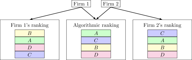
Figure 1: Each firm has the choice to use either their own private ranking or the common algorithmic ranking to order the $n$ candidates. In a random order, each firm hires the highest-ranked available candidate according to the ranking they chose. For example, if Firm 1 uses their private ranking and Firm 2 uses the algorithmic ranking, then Firm 1 hires candidate $B$ and Firm 2 hires candidate $A$. If both firms use the algorithmic ranking, then the firm randomly selected to hire first hires candidate $A$ and the firm randomly selected to hire second hires candidate $C$.

2 Algorithmic hiring as a case study

To instantiate the ideas introduced thus far, we’ll focus on the case of algorithmic hiring, where recruiters make decisions based in part on scores or recommendations provided by data-driven algorithms. In this setting, we’ll propose and analyze a stylized model of algorithmic hiring with which we can begin to investigate the effects of algorithmic monoculture.

Informally, we can think of a simplified hiring process as follows: rank all of the candidates and select the first available one. We suppose that each firm has two options to form this ranking: either develop their own, private ranking (which we will refer to as using a “human evaluator”), or use an algorithmically produced ranking. We assume that there is a single vendor of algorithmic rankings, so all firms choosing to use the algorithm receive the same ranking. The firms proceed in a random order, each hiring their favorite remaining candidate according to the ranking they’re using—human-generated or algorithmic (see Figure 1 for an example). Thus, we can frame the effects of monoculture as follows: are firms better off using the more accurate, common algorithm, or should they instead employ their own less accurate, but private, evaluations?

In what follows, we’ll introduce a formal model of evaluation and selection, using it to analyze a setting in which firms seek to hire candidates.

2.1 Modeling ranking

More formally, we model the $n$ candidates as having intrinsic values $x_{1},\dots,x_{n}$, where any employer would derive utility $x_{i}$ from hiring candidate $i$. Throughout the paper, we assume without loss of generality that $x_{1}>x_{2}>\dots>x_{n}$. These values, however, are unknown to the employer; instead, they must use some noisy procedure to rank the candidates. We model such a procedure as a randomized mechanism $\mathcal{R}$ that takes in the true candidate values and draws a permutation $\pi$ over those candidates from some distribution. Our main results hold for families of distributions over permutations as defined below:

Definition 1 (Noisy permutation family).

A noisy permutation family $\mathcal{F}_{\theta}$ is a family of distributions over permutations that satisfies the following conditions for any $\theta>0$ and set of candidates $\mathbf{x}$:

1. (Differentiability) For any permutation $\pi$, $\Pr_{\mathcal{F}_{\theta}}[\pi]$ is continuous and differentiable in $\theta$.

2. (Asymptotic optimality) For the true ranking $\pi^{*}$, $\lim_{\theta\to\infty}\Pr_{\mathcal{F}_{\theta}}[\pi^{*}]=1$.

3. (Monotonicity) For any (possibly empty) $S\subset\mathbf{x}$, let $\pi^{(-S)}$ be the partial ranking produced by removing the items in $S$ from $\pi$. Let $\pi_{1}^{(-S)}$ denote the value of the top-ranked candidate according to $\pi^{(-S)}$. For any $\theta^{\prime}>\theta$,

   $$\mathbb{E}_{\mathcal{F}_{\theta^{\prime}}}\left[\pi_{1}^{(-S)}\right]\geq\mathbb{E}_{\mathcal{F}_{\theta}}\left[\pi_{1}^{(-S)}\right].$$ (1)

   Moreover, for $S=\emptyset$, (1) holds with strict inequality.

$\theta$ serves as an “accuracy parameter”: for large $\theta$, the noisy ranking converges to the true ranking over candidates. The monotonicity condition states that a higher value of $\theta$ leads to a better first choice, even if some of the candidates are removed after ranking. Removal after ranking (as opposed to before) is important because some of the ranking models we will consider later do not satisfy Independence of Irrelevant Alternatives. Examples of noisy permutation families include Random Utility Models [23] and the Mallows Model [14], both of which we will discuss in detail later.

As an objective function to evaluate the effects of different approaches to ranking and selection, we’ll consider each individual employer’s utility as well as the sum of employers’ utilities. We think of this latter sum as the social welfare, since it represents the total quality of the applicants who are hired by any firm. (For example, if all firms deterministically used the correct ranking, then the top applicants would be the ones hired, leading to the highest possible social welfare.)

2.2 Modeling selection

Each firm in our model has access to the same underlying pool of $n$ candidates, which they rank using a randomized mechanism $\mathcal{R}$ to get a permutation $\pi$ as described above. Then, in a random order, each firm hires the highest-ranked remaining candidate according to their ranking. Thus, if two firms both rank candidate $i$ first, only one of them can hire $i$; the other must hire the next available candidate according to their ranking. In our model, candidates automatically accept the offer they get from a firm. For the sake of simplicity, throughout this paper, we restrict ourselves to the case where there are two firms hiring one candidate each, although our model readily generalizes to more complex cases.

As described earlier, each firm can choose to use either a private “human evaluator” or an algorithmically generated ranking as its randomized mechanism $\mathcal{R}$. We assume that both candidate mechanisms come from a noisy permutation family $F_{\theta}$, with differing values of the accuracy parameter $\theta$: human evaluators all have the same accuracy $\theta_{H}$, and the algorithm has accuracy $\theta_{A}$. However, while the human evaluator produces a ranking independent of any other firm, the algorithmically generated ranking is identical for all firms who choose to use it. In other words, if two firms choose to use the algorithmically generated ranking, they will both receive the same permutation $\pi$.

The choice of which ranking mechanism to use leads to a game-theoretic setting: both firms know the accuracy parameters of the human evaluators ($\theta_{H}$) and the algorithm ($\theta_{A}$), and they must decide whether to use a human evaluator or the algorithm. This choice introduces a subtlety: for many ranking models, a firm’s rational behavior depends not only on the accuracy of the ranking mechanism, but also on the underlying candidate values $x_{1},\dots,x_{n}$. Thus, to fully specify a firm’s behavior, we assume that $x_{1},\dots,x_{n}$ are drawn from a known joint distribution $\mathcal{D}$. Our main results will hold for any $\mathcal{D}$, meaning they apply even when the candidate values (but not their identities) are deterministically known.

2.3 Stating the main result

Our main result is a pair of intuitive conditions under which a Braess’ Paradox-style result occurs—in other words, conditions under which there are accuracy parameters for which both firms rationally choose to use the algorithmic ranking, but social welfare (and each individual firm’s utility) would be higher if both firms used independent human evaluators. Recall that the two firms hire in a random order. For a permutation $\pi$, let $\pi_{i}$ denote the value of the $i$th-ranked candidate according to $\pi$.

We first state the two conditions, and then the theorem based on them.

Definition 2 (Preference for the first position.).

A candidate distribution $\mathcal{D}$ and noisy permutation family $\mathcal{F}_{\theta}$ exhibits a preference for the first position if for all $\theta>0$, if $\pi,\sigma\sim\mathcal{F}_{\theta}$,

$$\mathbb{E}\left[\pi_{1}-\pi_{2}\;|\;\pi_{1}\neq\sigma_{1}\right]>0.$$

In other words, for any $\theta>0$, suppose we draw two permutations $\pi$ and $\sigma$ independently from $F_{\theta}$, and suppose that the first-ranked candidates differ in $\pi$ and $\sigma$. Then the expected value of the first-ranked candidate in $\pi$ is strictly greater than the expected value of the second-ranked candidate in $\pi$.

Definition 3 (Preference for weaker competition.).

A candidate distribution $\mathcal{D}$ and noisy permutation family $\mathcal{F}_{\theta}$, exhibits a preference for weaker competition if the following holds: for all $\theta_{1}>\theta_{2}$, $\sigma\sim\mathcal{F}_{\theta_{1}}$ and $\pi,\tau\sim\mathcal{F}_{\theta_{2}}$,

$$\mathbb{E}\left[\pi_{1}^{(-\{\sigma_{1}\})}\right]<\mathbb{E}\left[\pi_{1}^{(-\{\tau_{1}\})}\right].$$

Intuitively, suppose we have a higher accuracy parameter $\theta_{1}$ and a lower accuracy parameter $\theta_{2}<\theta_{1}$; we draw a permutation $\pi$ from $\mathcal{F}_{\theta_{2}}$; and we then derive two permutations from $\pi$: $\pi^{(-\{\sigma_{1}\})}$ obtained by deleting the first-ranked element of a permutation $\sigma$ drawn from the more accurate distribution $\mathcal{F}_{\theta_{1}}$, and $\pi^{(-\{\tau_{1}\})}$ obtained by deleting the first-ranked element of a permutation $\tau$ drawn from the less accurate distribution $\mathcal{F}_{\theta_{2}}$.

Then the expected value of the first-ranked candidate in $\pi^{(-\{\tau_{1}\})}$ is strictly greater than the expected value of the first-ranked candidate in $\pi^{(-\{\sigma_{1}\})}$ — that is, when a random candidate is removed from $\pi$, the best remaining candidate is better in expectation when the randomly removed candidate is chosen based on a noisier ranking.

Using these two conditions, we can state our theorem.

Theorem 1.

Suppose that a given candidate distribution $\mathcal{D}$ and noisy permutation family $\mathcal{F}_{\theta}$ satisfy Definition 2 (preference for the first position) and Definition 3 (preference for weaker competition).

Then, for any $\theta_{H}$, there exists $\theta_{A}>\theta_{H}$ such that using the algorithmic ranking is a strictly dominant strategy for both firms, but social welfare would be higher if both firms used human evaluators.

2.4 A Preference for Independence

Before we prove Theorem 1, we provide some intuition for the two conditions in Definitions 2 and 3. The second condition essentially says that it is better to have a worse competitor: the firm randomly selected to hire second is better off if the firm that hires first uses a less accurate ranking (in this case, a human evaluator instead of the algorithmic ranking).

The first condition states that when two identically distributed permutations disagree on their first element, the first-ranked candidate according to either permutation is still better, in expectation, than the second-ranked candidate according to either permutation. In what follows, we’ll demonstrate that this condition implies that firms in our model rationally prefer to make decisions using independent (but equally accurate) rankings.

To do so, we need to introduce some notation. Recall that the two firms hire in a random order. Given a candidate distribution $\mathcal{D}$, let $U_{s}(\theta_{A},\theta_{H})$ denote the expected utility of the first firm to hire a candidate when using ranking $s$, where $s\in\{A,H\}$ is either the algorithmic ranking or the ranking generated by a human evaluator respectively. Similarly, let $U_{s_{1}s_{2}}(\theta_{A},\theta_{H})$ be the expected utility of the second firm to hire given that the first firm used strategy $s_{1}$ and the second firm uses strategy $s_{2}$, where again $s_{1},s_{2}\in\{A,H\}$. Finally, let $\pi,\sigma\sim\mathcal{F}_{\theta}$.

In what follows, we will show that for any $\theta$,

$$\mathbb{E}\left[\pi_{1}-\pi_{2}\;|\;\pi_{1}\neq\sigma_{1}\right]>0\Longleftrightarrow U_{AH}(\theta,\theta)>U_{AA}(\theta,\theta).$$ (2)

In other words, whenever a ranking model meets Definition 2, the firm chosen to select second will prefer to use an independent ranking mechanism from it’s competitor, given that the ranking mechanisms are equally accurate.

First, we can write

$$U_{AH}(\theta_{A},\theta_{H}) =\mathbb{E}\left[\pi_{1}\cdot\mathbbm{1}_{\pi_{1}\neq\sigma_{1}}+\pi_{2}\cdot\mathbbm{1}_{\pi_{1}=\sigma_{1}}\right]$$

$$U_{AA}(\theta_{A},\theta_{H}) =\mathbb{E}\left[\sigma_{2}\right]$$

$$=\mathbb{E}\left[\sigma_{2}\cdot\mathbbm{1}_{\pi_{1}\neq\sigma_{1}}+\sigma_{2}\cdot\mathbbm{1}_{\pi_{1}=\sigma_{1}}\right]$$

Thus,

$$U_{AH}(\theta_{A},\theta_{H}) -U_{AA}(\theta_{A},\theta_{H})$$

$$=\mathbb{E}\left[(\pi_{1}-\sigma_{2})\cdot\mathbbm{1}_{\pi_{1}\neq\sigma_{1}}+(\pi_{2}-\sigma_{2})\cdot\mathbbm{1}_{\pi_{1}=\sigma_{1}}\right].$$

Conditioned on either $\pi_{1}=\sigma_{1}$ or $\pi_{1}\neq\sigma_{1}$, $\pi_{2}$ and $\sigma_{2}$ are identically distributed and therefore have equal expectations. As a result,

$$U_{AH}(\theta_{A},\theta_{H})-U_{AA}(\theta_{A},\theta_{H})=\mathbb{E}\left[(\pi_{1}-\pi_{2})\cdot\mathbbm{1}_{\pi_{1}\neq\sigma_{1}}\right],$$ (3)

which implies (2). Thus, whenever a ranking model meets Definition 2, firms rationally prefer independent assessments, all else equal.

To provide some intuition for what this preference for independence entails, consider a setting where a hiring committee seeks to hire two candidates. They meet, produce a ranking $\sigma$, and hire $\sigma_{1}$ (the best candidate according to $\sigma$). Suppose they have the option to either hire $\sigma_{2}$ or reconvene the next day to form an independent ranking $\pi$ and hire the best remaining candidate according to $\pi$; which option should they choose? It’s not immediately clear why one option should be better than the other. However, whenever Definition 2 is met, the committee should prefer to reconvene and make their second hire according to a new ranking $\pi$. After proving Theorem 1, we will provide natural ranking models that meet Definition 2, implying that under these ranking models, independent re-ranking can be beneficial.

2.5 Proving Theorem 1

With this intuition, we are ready to prove Theorem 1.

Proof of Theorem 1.

For given values of $\theta_{A}$ and $\theta_{H}$, using the algorithmic ranking is a strictly dominant strategy as long as

$$U_{A}(\theta_{A},\theta_{H})+U_{AA}(\theta_{A},\theta_{H}) >U_{H}(\theta_{A},\theta_{H})+U_{AH}(\theta_{A},\theta_{H})$$ (4)

$$U_{A}(\theta_{A},\theta_{H})+U_{HA}(\theta_{A},\theta_{H}) >U_{H}(\theta_{A},\theta_{H})+U_{HH}(\theta_{A},\theta_{H})$$ (5)

Note that (5) is always true for $\theta_{A}>\theta_{H}$ by the monotonicity assumption on $\mathcal{F}_{\theta}$: $U_{A}(\theta_{A},\theta_{H})\geq U_{H}(\theta_{A},\theta_{H})$ because a more accurate ranking produces a top-ranked candidate with higher expected value, and $U_{HA}(\theta_{A},\theta_{H})\geq U_{HH}(\theta_{A},\theta_{H})$ because this holds even conditioned on removing any candidate from the pool (in this case, the candidate randomly selected by the firm that hires first). Crucially, in (5), the first firm’s random selection is independent from the second firm’s selection; the same logic could not be used to argue that (4) always holds for $\theta_{A}\geq\theta_{H}$. Moreover, when $\theta_{A}>\theta_{H}$, $U_{A}(\theta_{A},\theta_{H})>U_{H}(\theta_{A},\theta_{H})$ by the monotonicity assumption, meaning (5) holds.

Let $W_{s_{1}s_{2}}(\theta_{A},\theta_{H})$ denote social welfare when the two firms employ strategies $s_{1},s_{2}\in\{A,H\}$. Then, when both firms use the algorithmic ranking, social welfare is

$$W_{AA}(\theta_{A},\theta_{H})=U_{A}(\theta_{A},\theta_{H})+U_{AA}(\theta_{A},\theta_{H}).$$

By (2), Definition 2 implies that for any $\theta$, $U_{AA}(\theta,\theta)<U_{AH}(\theta,\theta)$, implying

$$U_{A}(\theta_{H},\theta_{H})+U_{AA}(\theta_{H},\theta_{H})<U_{H}(\theta_{H},\theta_{H})+U_{AH}(\theta_{H},\theta_{H}).$$

However, by the optimality assumption on $\mathcal{F}_{\theta}$ in Definition 1, for sufficiently large $\hat{\theta}_{A}$,

$$U_{A}(\hat{\theta}_{A},\theta_{H})+U_{AA}(\hat{\theta}_{A},\theta_{H})>U_{H}(\hat{\theta}_{A},\theta_{H})+U_{AH}(\hat{\theta}_{A},\theta_{H}).$$

Note that $U_{s_{1}}(\theta_{A},\theta_{H})$ and $U_{s_{1}s_{2}}(\theta_{A},\theta_{H})$ are continuous with respect to $\theta_{A}$ for any $s_{1},s_{2}\in\{A,H\}$ since they are expectations over discrete distributions with probabilities that are by assumption differentiable with respect to $\theta_{A}$. Therefore, by the Differentiability assumption on $\mathcal{F}_{\theta}$ from Definition 1, there is some $\theta_{A}^{*}>\theta_{H}$ such that

$$U_{A}(\theta_{A}^{*},\theta_{H})+U_{AA}(\theta_{A}^{*},\theta_{H})=U_{H}(\theta_{A}^{*},\theta_{H})+U_{AH}(\theta_{A}^{*},\theta_{H}),$$ (6)

i.e., given that its competitor uses the algorithmic ranking, a firm is indifferent between the two strategies. For such $\theta_{A}^{*}$, using the algorithmic ranking is still a weakly dominant strategy. By definition of $W_{AA}$,

$$W_{AA}(\theta_{A}^{*},\theta_{H}) =U_{H}(\theta_{A}^{*},\theta_{H})+U_{AH}(\theta_{A}^{*},\theta_{H}).$$

If both firms had instead used human evaluators, social welfare would be

$$W_{HH}(\theta_{A}^{*},\theta_{H})=U_{H}(\theta_{A}^{*},\theta_{H})+U_{HH}(\theta_{A}^{*},\theta_{H}).$$

By Definition 3, for $\sigma\sim\mathcal{F}_{\theta_{A^{*}}}$ and $\pi,\tau\sim\mathcal{F}_{\theta_{H}}$,

$$\mathbb{E}\left[\pi_{1}^{(-\{\sigma_{1}\})}\right]<\mathbb{E}\left[\pi_{1}^{(-\{\tau_{1}\})}\right].$$

Note that

$$U_{AH}(\theta_{A}^{*},\theta_{H}) =\mathbb{E}\left[\pi_{1}^{(-\{\sigma_{1}\})}\right]$$

$$U_{HH}(\theta_{A}^{*},\theta_{H}) =\mathbb{E}\left[\pi_{1}^{(-\{\tau_{1}\})}\right]$$

Thus, Definition 3 implies that for $\theta_{A^{*}}>\theta_{H}$, $U_{HH}(\theta_{A}^{*},\theta_{H})>U_{AH}(\theta_{A}^{*},\theta_{H})$. As a result for $\theta_{A^{*}}>\theta_{H}$, using the algorithmic ranking is a weakly dominant strategy, but

$$W_{HH}(\theta_{A}^{*},\theta_{H}) =U_{H}(\theta_{A}^{*},\theta_{H})+U_{HH}(\theta_{A}^{*},\theta_{H})$$

$$>U_{H}(\theta_{A}^{*},\theta_{H})+U_{AH}(\theta_{A}^{*},\theta_{H})$$

$$=U_{A}(\theta_{A}^{*},\theta_{H})+U_{AA}(\theta_{A}^{*},\theta_{H})$$

$$=W_{AA}(\theta_{A}^{*},\theta_{H}),$$

meaning social welfare would have been higher had both firms used human evaluators.

We can show that this effect persists for a value $\theta_{A}^{\prime}$ such that using the algorithmic ranking is a strictly dominant strategy. Intuitively, this is simply by slightly increasing $\theta_{A}^{*}$ so the algorithmic ranking is strictly dominant. For fixed $\theta_{H}$, define

$$f(\theta_{A}) =U_{A}(\theta_{A},\theta_{H})+U_{AA}(\theta_{A},\theta_{H})$$

$$g(\theta_{A}) =U_{H}(\theta_{A},\theta_{H})+U_{AH}(\theta_{A},\theta_{H})$$

$$h(\theta_{A}) =U_{H}(\theta_{A},\theta_{H})+U_{HH}(\theta_{A},\theta_{H})$$

Because (5) always holds for $\theta_{A}>\theta_{H}$, it suffices to show that there exists $\theta_{A}^{\prime}$ such that $g(\theta_{A}^{\prime})<f(\theta_{A}^{\prime})<h(\theta_{A}^{\prime})$. This is because $g(\theta_{A}^{\prime})<f(\theta_{A}^{\prime})$ is equivalent to (4) and $f(\theta_{A}^{\prime})<h(\theta_{A}^{\prime})$ is equivalent to $W_{AA}(\theta_{A}^{\prime},\theta_{H})<W_{HH}(\theta_{A}^{\prime},\theta_{H})$.

First, note that $h(\theta_{A})$ is a constant, and by Definition 3, $g(\theta_{A})<h(\theta_{A})$ for all $\theta_{A}>\theta_{H}$. By the optimality assumption of Definition 1, there exists sufficiently large $\hat{\theta}_{A}$ such that $f(\hat{\theta}_{A})>g(\hat{\theta}_{A})$. Recall that by definition of $\theta_{A}^{*}$, $f(\theta_{A}^{*})=g(\theta_{A}^{*})$. Both $f$ and $g$ are continuous by the Differentiability assumption in Definition 1. Thus, there must exist some $\theta_{A}^{\prime}>\theta_{A}^{*}$ such that $g(\theta_{A}^{\prime})<f(\theta_{A}^{\prime})<h(\theta_{A}^{\prime})$. This means that for $\theta_{A}^{\prime}$, using the algorithmic ranking is a strictly dominant strategy, but social welfare would still be larger if both firms used human evaluators. ∎

3 Instantiating with Ranking Models

Thus far, we have described a general set of conditions under which algorithmic monoculture can lead to a reduction in social welfare. Under which ranking models do these conditions hold? In the remainder of this paper, we instantiate the model with two well-studied ranking models: Random Utility Models (RUMs) [23] and the Mallows Model [14]. While RUMs do not always satisfy Definitions 2 and 3, they do under some realistic parameterizations, regardless of the candidate distribution $\mathcal{D}$. Under the Mallows Model, Definitions 2 and 3 are always met, meaning that for any candidate distribution $\mathcal{D}$ and human evaluator accuracy $\theta_{H}$, there exists an accuracy parameter $\theta_{A}$ such that a common algorithmic ranking with accuracy $\theta_{A}$ decreases social welfare.

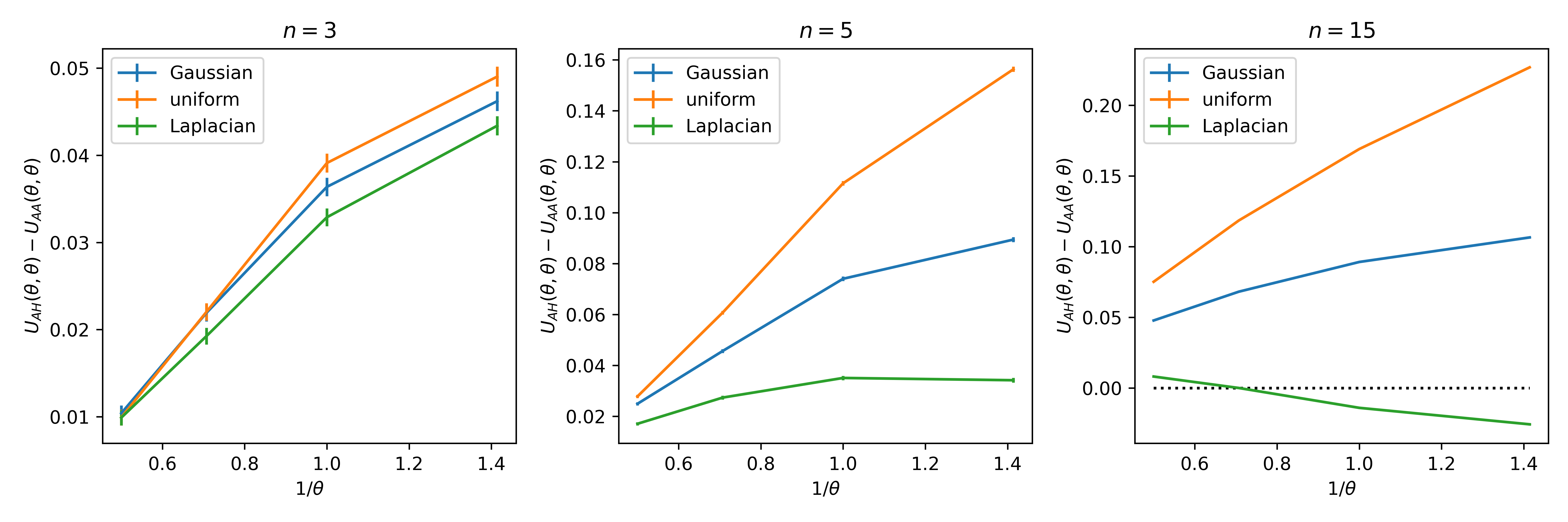
Figure 2: $U_{AH}(\theta,\theta)-U_{AA}(\theta,\theta)$ for three noise models with $n$ candidates whose utilities are drawn from a uniform distribution with unit variance for $n=3$, $n=5$, and $n=15$. Note that for $n=15$, $U_{AH}(\theta,\theta)-U_{AA}(\theta,\theta)<0$ for Laplacian noise, meaning Definition 2 is not met.

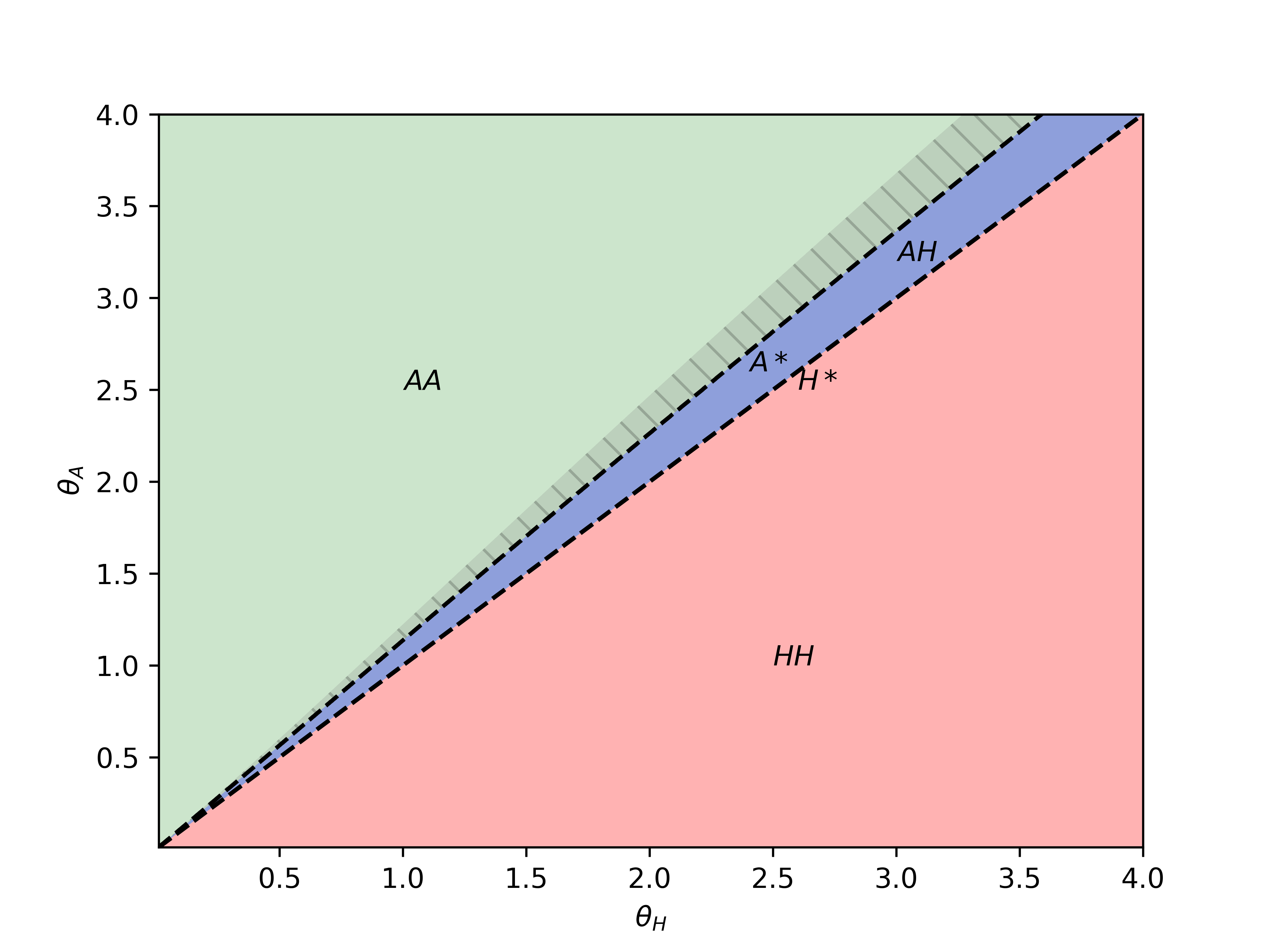
Figure 3: Regions for different equilibria. When human evaluators are more accurate than the algorithm, both firms decide to employ humans (HH). When the algorithm is significantly more accurate, both firms use the algorithm (AA). When the algorithm is slightly more accurate than human evaluators, two possible equilibria exist: (1) one firm uses the algorithm and the other employs a human (AH), or (2) both decide whether to use the algorithm with some probability $p$. The shaded portion of the green $AA$ region depicts where social welfare is smaller at the $AA$ equilibrium than it would be if both firms used human evaluators.

3.1 Random Utility Models

In Random Utility Models, the underlying candidate values $x_{i}$ are perturbed by independent and identically distributed noise $\varepsilon_{i}\sim\mathcal{E}$, and the perturbed values are ranked to produce $\pi$. Originally conceived in the psychology literature [23], this model has been well-studied over nearly a century, [7, 4, 9, 24, 16, 22], including more recently in the computer science and machine learning literature [2, 1, 19, 25, 13].

First, we must define a family of RUMs that satisfies the conditions of Definition 1. Assume without loss of generality that the noise distribution $\mathcal{E}$ has unit variance. Then, consider the family of RUMs parameterized by $\theta$ in which candidates are ranked according to $x_{i}+\frac{\varepsilon_{i}}{\theta}$. By this definition, the standard deviation of the noise for a particular value of $\theta$ is simply $1/\theta$. Intuitively, larger values of $\theta$ reduce the effect of the noise, making the ranking more accurate. In Theorem 5 in Appendix A, we show as long as the noise distribution $\mathcal{E}$ has positive support on $(-\infty,\infty)$, this definition of $\mathcal{F}_{\theta}$ meets the differentiability, asymptotic optimality, and monotonicity conditions in Definition 1. For distributions with finite support, many of our results can be generalized by relaxing strict inequalities in Definition 1 and Theorem 1 to weak inequalities.

Because RUMs are notoriously difficult to work with analytically, we restrict ourselves to the case where $n=3$, i.e., there are 3 candidates. Under this restriction, we can show that for Gaussian and Laplacian noise distributions, Definition 2 and 3 — the two conditions of Theorem 1 — are met, regardless of the candidate distribution $\mathcal{D}$. We defer the proof to Appendix C.

Theorem 2.

Let $\mathcal{F}_{\theta}$ be the family of RUMs with either Gaussian or Laplacian noise with standard deviation $1/\theta$. Then, for any candidate distribution $\mathcal{D}$ over 3 candidates, the conditions of Theorem 1 are satisfied.

It might be tempting to generalize Theorem 2 to other distributions and more candidates; however, certain noise and candidate distributions violate the conditions of Theorem 1. Even for 3-candidate RUMs, there exist distributions for which each of the conditions is violated; we provide such examples in Appendix B.

Moreover, while Gaussian and Laplacian distributions provably meet Definitions 2 and 3 with only 3 candidates, this doesn’t necessarily extend to larger candidate sets. Figure 2 shows that Definition 2 can be violated under a particular candidate distribution $\mathcal{D}$ for Laplacian noise with 15 candidates. This challenges the intuition that independence is preferable—under some conditions, it can actually better in expectation for a firm to use the same algorithmic ranking as its competitor, even if an independent human evaluator is equally accurate overall. Unlike Theorem 2, which applies for any candidate distribution $\mathcal{D}$, certain noise models may violate Definition 2 only for particular $\mathcal{D}$. It is an open question as to whether Theorem 2 can be extended to larger numbers of candidates under Gaussian noise.

Finally, there exist noise distributions that violate Definition 2 for any candidate distribution $\mathcal{D}$. In particular, the RUM family defined by the Gumbel distribution is well-known to be equivalent to the Plackett-Luce model of ranking, which is generated by sequentially selecting candidate $i$ with probability

$$\frac{\exp(\theta x_{i})}{\sum_{j\in S}\exp(\theta x_{j})},$$ (7)

where $S$ is the set of remaining candidates [12, 4]. Under the Plackett-Luce model, for any $\theta$, $U_{AH}(\theta,\theta)=U_{AA}(\theta,\theta)$. To see this, suppose the firm that hires first selects candidate $i^{*}$. Then, the firm that hires second gets each candidate $i$ with probability given by (7) with $S=\{1,\dots,n\}\backslash i^{*}$. As a result, by (3), if $\pi,\sigma\sim\mathcal{F}_{\theta}$,

$$\mathbb{E}\left[\pi_{1}-\pi_{2}\;|\;\pi_{1}\neq\sigma_{1}\right]=0$$

for any candidate distribution $\mathcal{D}$, meaning the Plackett-Luce model never meets Definition 2. Thus, under the Plackett-Luce model, monoculture has no effect—the optimal strategy is always to use the best available ranking, regardless of competitors’ strategies.

Given the analytic intractability of most RUMs, it might appear that testing the conditions of Theorem 1, especially for a particular noise and candidate distributions, may not be possible; however, they can be efficiently tested via simulation: as long as the noise distribution $\mathcal{E}$ and the candidate distribution $\mathcal{D}$ can be sampled from, it is possible to test whether the conditions of Theorem 1 are satisfied. Thus, even if the conditions of Theorem 1 are not met for every candidate distribution $\mathcal{D}$, it is possible to efficiently determine whether they are met for any particular $\mathcal{D}$.

It is also interesting to ask about the magnitude of the negative impact produced by monoculture. Our model allows for the qualities of candidates to be either positive or negative (capturing the fact that a worker’s productivity can be either more or less than their cost to the firm in wages); using this, we can construct instances of the model in which the optimal social welfare is positive but the welfare under the (unique) monocultural equilibrium implied by Theorem 1 is negative. This is a strong type of negative result, in which sub-optimality reverses the sign of the objective function, and it means that in general we cannot compare the optimum and equilibrium by taking a ratio of two non-negative quantities, as is standard in Price of Anarchy results. However, as a future direction, it would be interesting to explore such Price of Anarchy bounds in special cases of the problem where structural assumptions on the input are sufficient to guarantee that the welfare at both the social optimum and the equilibrium are non-negative. As one simple example, if the qualities for three candidates are drawn independently from a uniform distribution centered at 0, and the noise distribution is Gaussian, then there exist parameters $\theta_{A}>\theta_{H}$ such that expected social welfare at the equilibrium where both firm use the algorithmic ranking is non-negative, and approximately $4\%$ less than it would be had both firms used human evaluators instead.

3.2 The Mallows Model

The Mallows Model also appears frequently in the ranking literature [8, 11], and is much more analytically tractable than RUMs. Under the Mallows Model, the likelihood of a permutation is related to its distance from the true ranking $\pi^{*}$:

$$\Pr[\pi]=\frac{1}{Z}\phi^{-d(\pi,\pi^{*})},$$ (8)

where $Z$ is a normalizing constant. In this model, $\phi>1$ is the accuracy parameter: the larger $\phi$ is, the more likely the ranking procedure is to output a ranking $\pi$ that is close to the true ranking $r$. To instantiate this model, we need a notion of distance $d(\cdot,\cdot)$ over permutations. For this, we’ll use Kendall tau distance, another standard notion in the literature, which is simply the number of pairs of elements in $\pi$ that are incorrectly ordered [10]. In Appendix D, we verify that the family of distributions $\mathcal{F}_{\theta}$ given by the Mallows Model satisfies Definition 1, defining $\theta=\phi-1$ (for consistency, so $\theta$ is well-defined on $(0,\infty)$).

In contrast to RUMs, the Mallows Model always satisfies the conditions of Theorem 1 for any candidate distribution $\mathcal{D}$, which we prove in Appendix E.

Theorem 3.

Let $\mathcal{F}_{\theta}$ be the family of Mallows Model distributions with parameter $\theta=\phi-1$. Then, for any candidate distribution $\mathcal{D}$, the conditions of Theorem 1 are satisfied.

Figure 3 characterizes firms’ rational behavior at equilibrium in the $(\theta_{H},\theta_{A})$ plane under the Mallows Model. The decrease in social welfare found in Theorem 3 is depicted by the shaded portion of the green region labeled $AA$, where social welfare would be higher if both firms used human evaluators.

While the result of Theorem 3 is certainly stronger than that of Theorem 2, in that it applies to all instances of the Mallows Model without restrictions, it should be interpreted with some caution. The Mallows Model does not depend on the underlying candidate values, so according to this model, monoculture can produce arbitrarily large negative effects. While insensitivity to candidate values may not necessarily be reasonable in practice, our results hold for any candidate distribution $\mathcal{D}$. Thus, to the extent that the Mallows Model can reasonably approximate ranking in particular contexts, our results imply that monoculture can have negative welfare effects.

4 Models with Multiple Firms

Our main focus in this work has been on models with two competing firms. However, it is also interesting to consider the case of more than two firms; we will see that the complex and sometimes counterintuitive effects that we found in the two-firm case are further enriched by additional phenomena. Primarily, we will present the result of computational experiments with the model, exposing some fundamental structural properties in the multi-firm problem for which a formal analysis remains an intriguing open problem. For concreteness, we will focus on a model in which rankings are drawn from the Mallows model. As before, each firm must choose to order candidates according to either an independent, human-produced ranking or an algorithmic ranking common to all firms who choose it. These rankings come from instances of the Mallows model with accuracy parameters $\phi_{H}$ and $\phi_{A}$ respectively as defined in (8).

Braess’ Paradox for $k>2$ firms.

First, we ask whether the Braess’ Paradox effect persists with $k>2$ firms. We find that it is possible to construct instances of the problem with $k>2$ for which Braess’ Paradox occurs — using an algorithmic evaluation is a dominant strategy, but social welfare would be higher if all firms used human evaluators instead. For example, suppose $n=4$, $k=3$, $\phi_{A}=2$, $\phi_{H}=1.75$, and candidate qualities are drawn from a uniform distribution on $[0,1]$. We find via computation that at equilibrium, each firm will rationally decide to use the algorithmic evaluator and experience utility $\approx.551$, but if all firms instead used human evaluators, they would experience utility $\approx.552$. Thus, Braess’ Paradox can occur for $k>2$ firms. Proving a generalization of Theorem 3, to show that Braess’ Paradox can occur for any candidate distribution $\mathcal{D}$ and any value of $\phi_{H}$ for $k>2$ firms remains an open question.

Sequential decision-making.

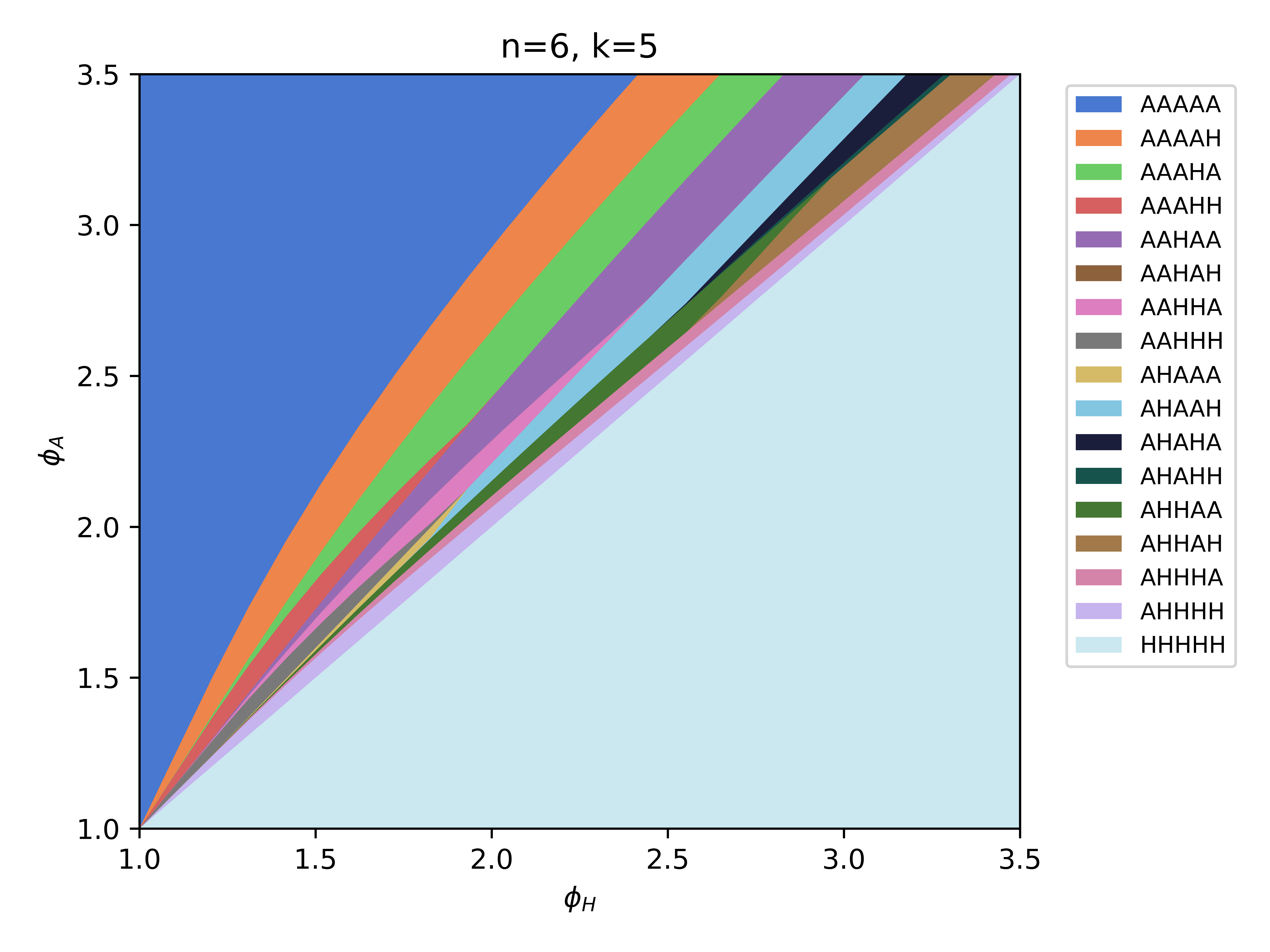
Figure 4: Regions for different optimal strategy profiles, where each strategy profile is a sequence of ‘$A$’ and ‘$H$’ representing the optimal strategies of each firm sequentially. For this plot, there are 5 firms ($k=5$) and 6 candidates ($n=6$) whose values are drawn from a uniform distribution. Note that when $\phi_{A}$ is much larger than $\phi_{H}$, all firms use the algorithmic ranking, but when $\phi_{A}$ is only slightly larger than $\phi_{H}$, only the first firm uses the algorithmic ranking.

Since the equilibrium behaviors we are studying take place in a model where firms make decisions in a random order, a crucial first step is to characterize firms’ optimal behavior when making decisions sequentially—that is, when firms hire in a fixed, known order as opposed to a random order. In this context, consider the rational behavior of each firm: given a distribution over candidate values, which ranking should each firm use? Clearly, the first firm to make a selection should use the more accurate ranking mechanism; however, as shown previously, subsequent firms’ decisions are less clear-cut. For a fixed number of firms, number of candidates, and distribution over candidate values, we can explore the firms’ optimal strategies over the possible space of $(\phi_{H},\phi_{A})$ values.

An optimal choice of strategies for the $k$ firms moving sequentially can be written as a sequence of length $k$ made up of the symbols $A$ and $H$; the $i^{\rm th}$ term in the sequence is equal to $A$ if the $i^{\rm th}$ firm to move sequentially uses the algorithm as its optimal strategy (given the choices of the previous $i-1$ firms), and it is equal to $H$ if the $i^{\rm th}$ firm uses an independent human evaluation. We can therefore represent the choice of optimal strategies, as the parameters $(\phi_{H},\phi_{A})$ vary, by a labeling of the $(\phi_{H},\phi_{A})$-plane: we label each point $(\phi_{H},\phi_{A})$ with the length-$k$ sequence that specifies the optimal sequence of strategies.

We can make the following initial formal observation about these optimal sequences:

Theorem 4.

When $\phi_{H}\geq\phi_{A}$, one optimal sequence is for all firms to choose $H$. When $\phi_{H}>\phi_{A}$, the unique optimal sequence is for all firms to choose $H$.

We prove this formally in Appendix F.1, but we provide a sketch here. When $\phi_{H}\geq\phi_{A}$, the first firm to move in sequence will simply use the more accurate strategy, and hence will choose $H$. Now, proceeding by induction, suppose that the first $i$ firms have all chosen $H$, and consider the $(i+1)^{\rm st}$ firm to move in sequence. Regardless of whether this firm chooses $A$ or $H$, it will be making a selection that is independent of the previous $i$ selections, and hence it is optimal for it to choose $H$ as well. Hence, by induction, it is an optimal solution for all firms to choose $H$ when $\phi_{H}\geq\phi_{A}$. (This argument, slightly adapted, also directly establishes that it is uniquely optimal for all firms to choose $H$ when $\phi_{H}>\phi_{A}$.)

Beyond this observation, if we wish to extend to the case when $\phi_{A}>\phi_{H}$, the mathematical analysis of this multi-firm model remains an open question; but it is possible to determine optimal strategies computationally for each choice of $(\phi_{H},\phi_{A})$, and then to look at how these strategies vary over the $(\phi_{H},\phi_{A})$-plane. Figure 4 shows the result of doing this — producing a labeling of the $(\phi_{H},\phi_{A})$-plane as described above — for $k=5$ firms and $n=6$ candidates, with the values of the candidates drawn from a uniform distribution.

We observe a number of interesting phenomena from this labeling of the plane. First, the region where $\phi_{H}\geq\phi_{A}$ is labeled with the all-$H$ sequence, reflecting the argument above; for the half-plane $\phi_{A}>\phi_{H}$, on the other hand, all optimal sequences begin with $A$, since it is always optimal for the first firm to use the more accurate method. The labeling of the half-plane $\phi_{A}>\phi_{H}$ becomes quite complex; in principle, any sequence over the binary alphabet $\{A,H\}$ that begins with $A$ could be possible, and in fact we see that all $2^{4}=16$ of these sequences appear as labels in some portion of the plane. This means that the sequential choice of optimal strategies for the firms can display arbitrary non-monotonicities in the choice of algorithmic or human decisions, with firms alternating between them; for example, even after the first firm chooses $A$ and the second chooses $H$, the third may choose $A$ or $H$ depending on the values $(\phi_{H},\phi_{A})$.

The boundaries of the regions labeled by different optimal sequences are similarly complex; some of the regions (such as $AAAHH$) appear to be bounded, while others (such as $AHAHA$ and $AHHAH$) appear to only emerge for sufficiently large values of $\phi_{H}$.

Perhaps the most intriguing observation about the arrangement of regions is the following. Suppose we think of the sequences of symbols over $\{A,H\}$ as binary representations of numbers, with $A$ corresponding to the binary digit $1$ and $H$ correspnding to the binary digit $0$. (Thus, for example, $AAAHH$ would correspond to the number $16+8+4=28$, while $AHAHA$ would correspond to the number $16+4+1=21$.) The observation is then the following: if we choose any vertical line $\phi_{H}=x$ (for a fixed $x$), and we follow it upward in the plane, we encounter regions in increasing order of the numbers corresponding to their labels, in this binary representation. (First $HHHHH$, then $AHHHH$, then $AHHHA$, then $AHHAH$, and so forth.)

We do not know a proof for this fact, or how generally it holds, but we can verify it computationally for the regions of the $(\phi_{H},\phi_{A})$-plane mapped out in Figure 4, as well as similar computational experiments not shown here for other choices of $k$ and $n$. This binary-counter property suggests a rich body of additional structure to the optimal strategies in the $k$-firm case, and we leave it as an open question to analyze this structure mathematically.

5 Conclusion

Concerns about monoculture in the use of algorithms have focused on the danger of unexpected, correlated shocks, and on the harm to particular individuals who may fare poorly under the algorithm’s decision. Our work here shows that concerns about algorithmic monoculture are in a sense more fundamental, in that it is possible for monoculture to cause decisions of globally lower average quality, even in the absence of shocks. In addition to telling us something about the pervasiveness of the phenomenon, it also suggests that it might be difficult to notice its negative effects even while they’re occurring — these effects can persist at low levels even without a shock-like disruption to call our attention to them. Our results also make clear that algorithmic monoculture in decision-making doesn’t always lead to adverse outcomes; rather, we given natural conditions under which such outcomes become possible, and show that these conditions hold in a wide range of standard models.

Our results suggest a number of natural directions for further work. To begin with, we have noted earlier in the paper that it would be interesting to give more comprehensive quantitative bounds on the magnitude of monoculture’s possible negative effects in decisions such as hiring — how much worse can the quality of candidates be when selected with an equilibrium strategy involving shared algorithms than with a socially optimal one? In formulating such questions, it will be important to take into account how the noise model for rankings relates to the numerical qualities of the candidates.

We have also focused here on the case of two firms and a single shared algorithm that is available to both. It would be natural to consider generalizations involving more firms and potentially more algorithms as well. With more algorithms, we might see solutions in which firms cluster around different algorithms of varying accuracies, as they balance the level of accuracy and the amount of correlation in their decisions. It would also be interesting to explore the ways in which correlations in firms’ decisions can be decomposed into constituent parts, such as the use of standardized tests that form input features for algorithms, and how quantifying these forms of correlation might help firms assess their decisions.

Finally, it will be interesting to consider how these types of results apply to further domains. While the analysis presented here illustrates the consequences of monoculture as applied to algorithmic hiring, our findings have potential implications in a broader range of settings. Algorithmic monoculture not only leads to a lack of heterogeneity in decision-making; by allowing valuable options to slip through the cracks — be they job candidates, potential hit songs, or budding entrepreneurs — it reduces total social welfare, even when the individual decisions are more accurate on a case-by-case basis. These concerns extend beyond the use of algorithms; whenever decision-makers rely on identical or highly correlated evaluations, they miss out on hidden gems, and in this way diminish the overall quality of their decisions.

Acknowledgements.

This work has been supported in part by a Simons Investigator Award, a Vannevar Bush Faculty Fellowship, a MURI grant, an NSF Graduate Research Fellowship, and grants from the ARO, AFOSR, and the MacArthur Foundation.

Appendix A Random Utility Models satisfying Definition 1

Theorem 5.

Let $f$ be the pdf of $\mathcal{E}$. The family of RUMs $\mathcal{F}_{\theta}$ given by ranking $x_{i}+\frac{\varepsilon_{i}}{\theta}$ with $\varepsilon_{i}\sim\mathcal{E}$ satisfies the conditions of Definition 1 if:

• $f$ is differentiable

• $f$ has positive support on $(-\infty,\infty)$

Proof.

We need to show that $\mathcal{F}_{\theta}$ satisfies the differentiability, asymptotic optimality, and monotonicity conditions in Definition 1.

Differentiability: The probability density of any realization of the $n$ noise samples $\varepsilon_{i}/\theta$ is $\prod_{i=1}^{n}f(\varepsilon_{i}/\theta)$. Let $\varepsilon=[\varepsilon_{1}/\theta,\dots,\varepsilon_{n}/\theta]$ be the vector of noise values and let $M(\pi)\subseteq\mathbb{R}^{n}$ be the region such that any $\varepsilon\in M(\pi)$ will produces the ranking $\pi$. The probability of any permutation $\pi$ is

$$\Pr_{\theta}[\pi]=\int_{M(\pi)}\prod_{i=1}^{n}f\left(\frac{\varepsilon_{i}}{\theta}\right)\;d^{n}\mathbf{z}.$$

Because $f$ is differentiable,

$$\frac{d}{d\theta}f\left(\frac{x}{\theta}\right)=f^{\prime}\left(\frac{x}{\theta}\right)\cdot\left(-\frac{x}{\theta^{2}}\right)$$

Because $\Pr{\theta}(\pi)$ is an integral of the product of differentiable functions over a fixed region, it is differentiable.

Asymptotic optimality: We will show that for any pair of elements and any $\delta>0$, there exists sufficiently large $\theta$ such that the probability that they incorrectly ranked is at most $\delta$. We will conclude with a union bound over the $n-1$ pairs of adjacent candidates that there exists sufficiently large $\theta$ such that the probability of outputting the correct ranking must be at least $1-(n-1)\delta$.

Consider two candidates $x_{i}>x_{i+1}$. Let $\nu$ be the difference $x_{i}-x_{i+1}$. Then, they will be correctly ranked if

$$\frac{\varepsilon_{i}}{\theta} >-\frac{\nu}{2}$$

$$\frac{\varepsilon_{i+1}}{\theta} <\frac{\nu}{2}$$

Let $\overline{q}$ and $\underline{q}$ be the $1-\frac{\delta}{2}$ and $\frac{\delta}{2}$ quantiles of $\mathcal{E}$ respectively, and let $q=\max(|\overline{q}|,|\underline{q}|)$. For $\theta>\frac{2q}{\nu}$,

$$\Pr\left[\frac{\varepsilon_{i}}{\theta}<-\frac{\nu}{2}\right] =\Pr\left[\varepsilon_{i}<-\frac{\nu\theta}{2}\right]$$

$$<\Pr\left[\varepsilon_{i}<-q\right]$$

$$\leq\Pr\left[\varepsilon_{i}<\underline{q}\right]$$

$$=\frac{\delta}{2}$$

$$\Pr\left[\frac{\varepsilon_{i+1}}{\theta}>\frac{\nu}{2}\right] =\Pr\left[\varepsilon_{i+1}>\frac{\nu\theta}{2}\right]$$

$$<\Pr\left[\varepsilon_{i+1}>q\right]$$

$$\leq\Pr\left[\varepsilon_{i+1}>\overline{q}\right]$$

$$=\frac{\delta}{2}$$

Thus, for sufficiently large $\theta$, the probability that $x_{i}$ and $x_{i+1}$ are incorrectly ordered is at most $\delta$.

Repeating this analysis for all $n-1$ pairs of adjacent elements, taking the maximum of all the $\theta$’s, and taking a union bound yields that the probability of incorrectly ordering any pair of elements is at most $(n-1)\delta$, meaning the probability of outputting the correct ranking is at least $1-(n-1)\delta$. Since $\delta$ is arbitrary, this probability can be made arbitrarily close to 1, satisfying the asymptotic optimality condition.

Monotonicity: The removal of any elements does not alter the distribution of the remaining elements, meaning that the distribution of $\pi^{(-S)}$ is equivalent to a RUM with $n-|S|$ elements. Thus, it suffices to show that for a RUM with positive support on $(-\infty,\infty)$, the probability of ranking the best candidate first strictly increases with $\theta$.

Recall that by definition, the candidates are ranked according to $x_{i}+\frac{\varepsilon_{i}}{\theta}$. The probability that $x_{1}$ is ranked first is

$$\Pr\left[x_{1}+\frac{\varepsilon_{1}}{\theta}>\max_{2\leq i\leq n}x_{i}+\frac{\varepsilon_{i}}{\theta}\right] =\Pr\left[\frac{\varepsilon_{1}}{\theta}>\max_{2\leq i\leq n}x_{i}-x_{1}+\frac{\varepsilon_{i}}{\theta}\right]$$

$$=\Pr\left[\varepsilon_{1}>\max_{2\leq i\leq n}\theta(x_{i}-x_{1})+\varepsilon_{i}\right]$$

$$=\mathbb{E}_{\varepsilon_{2},\dots,\varepsilon_{n}}\Pr\left[\varepsilon_{1}>\max_{2\leq i\leq n}\theta(x_{i}-x_{1})+\varepsilon_{i}\;|\;\varepsilon_{2},\dots,\varepsilon_{n}\right]$$ (A.1)

We want to show that (A.1) is increasing in $\theta$. Intuitively, this is because as $\theta$ increases, the right hand side of the inequality inside the probability decreases. To prove this formally, it suffices to show that the subderivative of (A.1) with respect to $\theta$ only includes strictly positive numbers. First, we have

$$\frac{\partial}{\partial\theta} \mathbb{E}_{\varepsilon_{2},\dots,\varepsilon_{n}}\Pr\left[\varepsilon_{1}>\max_{2\leq i\leq n}\theta(x_{i}-x_{1})+\varepsilon_{i}\;|\;\varepsilon_{2},\dots,\varepsilon_{n}\right]\subset\mathbb{R}_{>0}$$

$$\Longleftrightarrow\frac{\partial}{\partial\theta}\Pr\left[\varepsilon_{1}>\max_{2\leq i\leq n}\theta(x_{i}-x_{1})+\varepsilon_{i}\;|\;\varepsilon_{2},\dots,\varepsilon_{n}\right]\subset\mathbb{R}_{>0}$$

Let $F$ and $f$ be the cumulative density function and probability density function of $\mathcal{E}$ respectively. Then,

$$\Pr\left[\varepsilon_{1}>\max_{2\leq i\leq n}\theta(x_{i}-x_{1})+\varepsilon_{i}\;|\;\varepsilon_{2},\dots,\varepsilon_{n}\right]=1-F\left(\max_{2\leq i\leq n}\theta(x_{i}-x_{1})+\varepsilon_{i}\right)$$

Note that $F(\cdot)$ is strictly increasing (since $f$ is assumed to have positive support on $(-\infty,\infty)$), so it suffices to show that

$$\frac{\partial}{\partial\theta}\max_{2\leq i\leq n}\theta(x_{i}-x_{1})+\varepsilon_{i}\subset\mathbb{R}_{<0}$$

For any $i$,

$$\frac{d}{d\theta}\theta(x_{i}-x_{1})+\varepsilon_{i}=x_{i}-x_{1}<0.$$

Thus, the subderivative of the max of such functions includes only strictly negative numbers, which completes the proof. ∎

Appendix B 3-candidate RUM Counterexamples

B.1 Violating Definition 2

Here, we provide a noise mode $\mathcal{E}$, accuracy parameter $\theta$, and candidate distribution $\mathcal{D}$ such that $U_{AH}<U_{AA}$.

Choose the noise distribution $\mathcal{E}$ and accuracy parameter $\theta$ such that

$$\frac{\varepsilon}{\theta} =\begin{cases}1&w.p.\frac{\delta}{2}\\ 0&w.p.1-\delta\\ -1&w.p.\frac{\delta}{2}\end{cases}$$

Note that this distribution does not satisfy Definition 1 because it is neither differentiable nor supported on $(-\infty,\infty)$; however, we can provide a “smooth” approximation to this distribution by expressing it as the sum of arbitrarily tightly concentrated Gaussians with the same results.

We choose the candidate distribution $\mathcal{D}$ such that $x_{1}-1>x_{2}>x_{3}>x_{1}-2$. For example,

$$x_{1} =\frac{7}{4}$$

$$x_{2} =\frac{1}{2}$$

$$x_{3} =0$$

Under this condition, assuming $x_{3}=0$ without loss of generality,

$$U_{AH}(\theta,\theta)-U_{AA}(\theta,\theta)=\frac{\delta^{2}}{32}\left(\delta^{3}x_{1}-4\delta^{2}x_{1}+4\delta x_{1}+2\delta^{3}x_{2}-14\delta^{2}x_{2}+20\delta x_{2}-8x_{2}\right)$$

Notice that the lowest-power $\delta$ term is $-\frac{\delta^{2}x_{2}}{4}$. Therefore, for sufficiently small $\delta$, this is negative. For example, plugging in the values given above with $\delta=.1$, $U_{AH}(\theta,\theta)-U_{AA}(\theta,\theta)\approx-0.00076$.

B.2 Violating Definition 3

Next, we’ll give a 3-candidate RUM for which $U_{AH}<U_{HH}$ does not hold in general. Consider the following 3-candidate example.

$$x_{1} =3$$

$$x_{2} =2$$

$$x_{3} =0$$

Choose $\mathcal{E}$ and $\theta$ such that

$$\frac{\varepsilon}{\theta}=\begin{cases}1&\text{w.p.}~{}\frac{1-\delta}{2}\\ -1&\text{w.p.}~{}\frac{1-\delta}{2}\\ 10&\text{w.p.}~{}\frac{\delta}{2}\\ -10&\text{w.p.}~{}\frac{\delta}{2}\end{cases}$$

Again, while this noise model doesn’t satisfy Definition 1, we can approximate it arbitrarily closely with the sum of tightly concentrated Gaussians. Let the $\theta_{A}=1.1\theta$ and $\theta_{H}=0.9\theta$.

We will show that for these parameters, $U_{AH}(\theta_{A},\theta_{H})>U_{HH}(\theta_{A},\theta_{H})$, i.e., it is somehow better to choose after a better opponent than after a worse opponent. At a high level, the reasoning for this is as follows:

1. When choosing first, the only difference between the algorithm and the human evaluator is that the algorithm is more likely to choose $x_{2}$ than $x_{3}$. Both strategies have identical probabilities of selecting $x_{1}$.

2. When choosing second, the human evaluator’s utility is higher when $x_{2}$ has already been chosen than when $x_{3}$ has already been chosen. This is because when $x_{2}$ is unavailable, the human evaluator is almost guaranteed to get $x_{1}$; when $x_{3}$ is unavailable, the human evaluator will choose $x_{2}$ with probability $\approx 1/4$.

Let $\tau$ and $\pi$ be rankings generated by the algorithm and human evaluator respectively. First, we will show that

$$\Pr[\tau_{1}=x_{1}] =\Pr[\pi_{1}=x_{1}]$$ (B.1)

$$\Pr[\tau_{1}=x_{2}] >\Pr[\pi_{1}=x_{2}]$$ (B.2)

To do so, consider the realizations of $\varepsilon_{1},\varepsilon_{2},\varepsilon_{3}$ that result in different rankings under $\theta_{A}$ and $\theta_{H}$. In fact, the only set of realizations that result in different rankings are when $\varepsilon_{2}/\theta=-1$ and $\varepsilon_{3}/\theta=1$. Thus, the algorithm and human evaluator always rank $x_{1}$ in the same position, conditioned on a realization, which proves (B.1); the only difference is that the algorithm sometimes ranks $x_{2}$ above $x_{3}$ when the human evaluator does not. Moreover, whenever $\varepsilon_{1}/\theta=-10$, $x_{2}$ is more strictly more likely to be ranked first under the algorithm than the human evaluator, which proves (B.2).

Next, we must show that when choosing second, the human evaluator is better off when $x_{2}$ is unavailable than when $x_{3}$ is unavailable. This is clearly true because for the human evaluator,

$$\Pr\left[x_{1}+\frac{\varepsilon_{1}\theta_{H}}{\theta}>x_{3}+\frac{\varepsilon_{3}\theta_{H}}{\theta}\right] \approx 1-O(\delta)$$

$$\Pr\left[x_{1}+\frac{\varepsilon_{1}\theta_{H}}{\theta}>x_{2}+\frac{\varepsilon_{3}\theta_{H}}{\theta}\right] \approx\frac{3}{4}$$

Thus, conditioned on $x_{2}$ being unavailable, the human evaluator gets utility $\approx 3$, whereas when $x_{3}$ is unavailable, the human evaluator gets utility $\approx 2.75$. Let $u_{-i}$ be the expected utility for the human evaluator when $x_{i}$ is unavailable. Putting this together, we get

$$U_{AH} (\theta_{A},\theta_{H})-U_{HH}(\theta_{A},\theta_{H})$$

$$=\sum_{i=1}^{3}(\Pr[\tau_{1}=x_{i}]-\Pr[\pi_{1}=x_{i}])u_{-i}$$

$$=(\Pr[\tau_{1}=x_{1}]-\Pr[\pi_{1}=x_{1}])u_{-1}+(\Pr[\tau_{1}=x_{2}]-\Pr[\pi_{1}=x_{2}])u_{-2}+(\Pr[\tau_{1}=x_{3}]-\Pr[\pi_{1}=x_{3}])u_{-3}$$

$$=(\Pr[\tau_{1}=x_{2}]-\Pr[\pi_{1}=x_{2}])u_{-2}+(\Pr[\tau_{1}=x_{3}]-\Pr[\pi_{1}=x_{3}])u_{-3} \Pr[\tau_{1}=x_{1}=\Pr[\pi_{1}=x_{1}]$$ ()

$$=(\Pr[\tau_{1}=x_{2}]-\Pr[\pi_{1}=x_{2}])(u_{-2}-u_{-3}) \sum_{i=1}^{3}\Pr[\tau_{1}=x_{i}]=\sum_{i=1}^{3}\Pr[\pi_{1}=x_{i}]$$ ()

$$>0$$

The last step follows from (B.2) and because $u_{-2}>u_{-3}$.

Appendix C Proof of Theorem 2

C.1 Verifying Definition 2

By (2), we can equivalently show that for any $\theta$, $U_{AH}(\theta,\theta)>U_{AA}(\theta,\theta)$. Let $\tau$ and $\pi$ be the algorithmic and human-generated rankings respectively. Note that they’re identically distributed because $\theta_{A}=\theta_{H}$. Define

$$Y\triangleq\begin{cases}\pi_{1}&\pi_{1}\neq\tau_{1}\\ \pi_{2}&\text{otherwise}\end{cases}$$

Note that $U_{AH}(\theta,\theta)=\mathbb{E}\left[Y\right]$ and $U_{AA}(\theta,\theta)=\mathbb{E}\left[\tau_{2}\right]$. We want to show that $U_{AH}(\theta,\theta)-U_{AA}(\theta,\theta)=\mathbb{E}\left[x_{Y}-x_{\tau_{2}}\right]>0$. It is sufficient to show that for any $k$, $\mathbb{E}\left[Y-\tau_{2}\;|\;\tau_{1}=x_{k}\right]>0$. Let $X_{i}=x_{i}+\varepsilon_{i}/\theta$. Note that for distinct $i,j,k$ and $x_{i}>x_{j}$,

$$\mathbb{E}\left[Y-\tau_{2}\;|\;\tau_{1}=x_{k}\right]>0 \Longleftarrow\frac{\Pr[Y=x_{i}\;|\;\tau_{1}=x_{k}]}{\Pr[Y=x_{j}\;|\;\tau_{1}=x_{k}]}>\frac{\Pr[\tau_{2}=x_{i}\;|\;\tau_{1}=x_{k}]}{\Pr[\tau_{2}=x_{j}\;|\;\tau_{1}=x_{k}]}$$

$$\Longleftrightarrow\Pr[Y=x_{i}\;|\;\tau_{1}=x_{k}]>\Pr[\tau_{2}=x_{i}\;|\;\tau_{1}=x_{k}]$$ (numerator and denominator sum to 1)

$$\Longleftrightarrow\Pr[X_{i}>X_{j}]>\Pr[X_{i}>X_{j}\;|\;X_{k}>X_{i}\cap X_{k}>X_{j}]$$

$$\Longleftrightarrow\Pr[X_{i}>X_{j}]>\mathbb{E}_{X_{k}}[\Pr[X_{i}>X_{j}\;|\;X_{k}=a,X_{i}<a,X_{j}<a]].$$

Thus, it suffices to show that for any $a$,

$$\Pr[X_{i}>X_{j}]>\Pr[X_{i}>X_{j}\;|\;X_{i}<a,X_{j}<a].$$ (C.1)

Since $\Pr[X_{i}>X_{j}]=\lim_{a\to\infty}\Pr[X_{i}>X_{j}\;|\;X_{i}<a,X_{j}<a]$, it suffices to show that for all $a$,

$$\frac{d}{da}\Pr[X_{i}>X_{j}\;|\;X_{i}<a,X_{j}<a]\geq 0,$$ (C.2)

and that it is strictly positive for some $a$. In other words, the higher $a$ is, the more likely $i$ and $j$ are to be correctly ordered. In Theorems 7 and 8, we show that (C.2) holds for both Laplacian and Gaussian noise respectively, which proves that RUMs based on both distributions satisfy Definition 2.

C.2 Verifying Definition 3

Next, we show that for both Laplacian and Gaussian distributions, $U_{AH}(\theta_{A},\theta_{H})<U_{HH}(\theta_{A},\theta_{H})$ for all $\theta_{A}>\theta_{H}$. In fact, for 3-candidate RUM families, we will show that this is always true for any well-ordered distribution, defined as follows.

Definition 4.

A noise model with density $f(\cdot)$ is well-ordered if for any $a>b$ and $c>d$,

$$f(a-c)f(b-d)>f(a-d)f(b-c).$$

In other words, for a well-ordered noise model, given two numbers, two candidates are more likely to be correctly ordered than inverted conditioned on realizing those two numbers in some order. Lemma 1 shows that both Gaussian and Laplacian distributions are well-ordered.

Thus, it suffices to show that for any 3-candidate RUM with a well-ordered noise model, $U_{AH}(\theta_{A},\theta_{H})<U_{HH}(\theta_{A},\theta_{H})$ when $\theta_{A}>\theta_{H}$.

Theorem 6.

For 3 candidates with unique values $x_{1}>x_{2}>x_{3}$ and well-ordered i.i.d. noise with support $(-\infty,\infty)$, if $\theta_{A}>\theta_{H}$, then $U_{AH}(\theta_{A},\theta_{H})<U_{HH}(\theta_{A},\theta_{H})$.

Proof.

Define $u_{-i}$ to be the expected utility of the maximum element of the human-generated ranking when $i$ is not available. Because we’re in the 3-candidate setting, we have

$$u_{-1} =\lambda_{1}x_{2}+(1-\lambda_{1})x_{3}$$

$$u_{-2} =\lambda_{2}x_{1}+(1-\lambda_{2})x_{3}$$

$$u_{-3} =\lambda_{3}x_{1}+(1-\lambda_{3})x_{2}$$

where $1/2<\lambda_{i}<1$. This is because the noise has support everywhere, so it is impossible to correctly rank any two candidates with probability 1, and any two candidates are more likely than not to be correctly ordered:

$$\Pr\left[\frac{\varepsilon_{i}}{\theta}-\frac{\varepsilon_{j}}{\theta}>-\delta\right]=\Pr[\varepsilon_{i}-\varepsilon_{j}\geq 0]+\Pr\left[0>\frac{\varepsilon_{i}-\varepsilon_{j}}{\theta}>-\delta\right]>\frac{1}{2}$$

Note that $\lambda_{2}>\lambda_{1}$ and $\lambda_{2}>\lambda_{3}$, since

$$\lambda_{2}=\Pr[\varepsilon_{1}-\varepsilon_{3}>-\theta(x_{1}-x_{3})]>\max\left\{\Pr[\varepsilon_{1}-\varepsilon_{3}>-\theta(x_{2}-x_{3})],\Pr[\varepsilon_{1}-\varepsilon_{3}>-\theta(x_{1}-x_{2})]\right\}=\max\{\lambda_{1},\lambda_{3}\}.$$

Let $\tau\sim\mathcal{F}_{\theta_{A}}$ and $\pi\sim\mathcal{F}_{\theta_{H}}$. With this, we can write

$$U_{AH}(\theta_{A},\theta_{H}) =\sum_{i=1}^{3}\Pr[\tau_{1}=i]u_{-i}$$

$$U_{HH}(\theta_{A},\theta_{H}) =\sum_{i=1}^{3}\Pr[\pi_{1}=i]u_{-i}$$

Define

$$\Delta p_{i}=\Pr[\tau_{1}=i]-\Pr[\pi_{1}=i]$$

Using Lemmas 2, and 3, we have

$$\Delta p_{1} >0$$ (By monotonicity of RUM families, see Appendix A)

$$\Delta p_{1} \geq\Delta p_{2}$$

$$\Delta p_{3} \leq 0$$

Also, $\Delta p_{1}+\Delta p_{2}+\Delta p_{3}=0$. We must show that

$$U_{AH}(\theta_{A},\theta_{H})-U_{HH}(\theta_{A},\theta_{H})=\sum_{i=1}^{3}\Delta p_{i}u_{-i}<0.$$

We consider 2 cases.

Case 1: $\Delta p_{2}\leq 0$.
Then, $\Delta p_{1}=-(\Delta p_{2}+\Delta p_{3})$. This yields

$$\sum_{i=1}^{3}\Delta p_{i}u_{-i} =\Delta p_{1}u_{-1}+\Delta p_{2}u_{-2}+\Delta p_{3}u_{-3}$$

$$\leq\Delta p_{1}u_{-1}-\Delta p_{1}\min(u_{-2},u_{-3})$$

$$=\Delta p_{1}\left(\lambda_{1}x_{2}+(1-\lambda_{1})x_{3}-\min\left\{\lambda_{2}x_{1}+(1-\lambda_{2})x_{3},\lambda_{3}x_{1}+(1-\lambda_{3})x_{2}\right\}\right)$$

$$\leq\Delta p_{1}\left(\lambda_{1}x_{2}+(1-\lambda_{1})x_{3}-\min\left\{\lambda_{2}x_{1}+(1-\lambda_{2})x_{3},x_{2}\right\}\right)$$

We can show that this is at most 0 regardless of which term attains the minimum. Because $\lambda_{2}>\lambda_{1}$,

$$\lambda_{1}x_{2}+(1-\lambda_{1})x_{3}-\lambda_{2}x_{1}-(1-\lambda_{2})x_{3} =\lambda_{1}x_{2}+x_{3}-\lambda_{1}x_{3}-\lambda_{2}x_{1}-x_{3}+\lambda_{2}x_{3}$$

$$=\lambda_{1}x_{2}-\lambda_{1}x_{3}-\lambda_{2}x_{1}+\lambda_{2}x_{3}$$

$$=\lambda_{1}(x_{2}-x_{3})+\lambda_{2}(x_{3}-x_{1})$$

$$<\lambda_{1}(x_{2}-x_{3})+\lambda_{1}(x_{3}-x_{1})$$

$$=\lambda_{1}(x_{2}-x_{1})$$

$$<0$$

For the second term, we have

$$\lambda_{1}x_{2}+(1-\lambda_{1})x_{3}-x_{2}=(1-\lambda_{1})(x_{3}-x_{2})<0.$$

Thus,

$$\sum_{i=1}^{3}\Delta p_{i}u_{-i}<0.$$

Case 2: $\Delta p_{2}>0$. Note that $u_{-1}<x_{2}<u_{-3}$. Then, using $\Delta p_{3}=-(\Delta p_{1}+\Delta p_{2})$,

$$\sum_{i=1}^{3}\Delta p_{i}u_{-i} =\Delta p_{1}u_{-1}+\Delta p_{2}u_{-2}+\Delta p_{3}u_{-3}$$

$$=\Delta p_{1}(u_{-1}-u_{-3})+\Delta p_{2}(u_{-2}-u_{-3})$$

$$\leq\Delta p_{2}(u_{-1}-u_{-3})+\Delta p_{2}(u_{-2}-u_{-3}) \Delta p_{1}\geq\Delta p_{2} u_{-1}<u_{-3}$$ ( and )

$$=\Delta p_{2}(u_{-1}+u_{-2}-2u_{-3})$$

$$\leq\Delta p_{2}(x_{2}+x_{1}-2(\lambda_{3}x_{1}+(1-\lambda_{3})x_{2}))$$

$$<\Delta p_{2}\left(x_{2}+x_{1}-2\left(\frac{1}{2}x_{1}+\frac{1}{2}x_{2}\right)\right) \lambda_{3}>\frac{1}{2}$$ ()

$$=0$$

Thus, $U_{AH}(\theta_{A},\theta_{H})<U_{HH}(\theta_{A},\theta_{H})$. ∎

C.3 Supplementary Lemmas for Random Utility Models

Lemma 1.

Both Gaussian and Laplacian distributions are well-ordered.

Proof.

The Gaussian noise model is well-ordered:

$$f(a-c)f(b-d) =\frac{1}{2\sigma^{2}\pi}\exp(-(a-c)^{2}-(b-d)^{2})$$

$$=\frac{1}{2\sigma^{2}\pi}\exp(-(a-d)^{2}-(b-c)^{2}-2(ac+bd-ad-bc))$$

$$=f(a-d)f(b-c)\exp(-2((a-b)(c-d)))$$

$$<f(a-d)f(b-c)$$

Laplacian noise is as well:

$$f(a-c)f(b-d) =\frac{1}{4}\exp(-|a-c|-|b-d|)$$

$$f(a-d)f(b-c) =\frac{1}{4}\exp(-|a-d|-|b-c|)$$

It suffices to show that for $a>b$ and $c>d$, $|a-c|+|b-d|<|a-d|+|b-c|$. To show this, plot $(a,b)$ and $(c,d)$ in the $(x,y)$ plane. Note that they’re both below the $y=x$ line, and that the $\ell_{1}$ distance between them is $|a-c|+|b-d|$. Moreover, the $\ell_{1}$ distance between any two points must be realized by some Manhattan path, which is a combination of horizontal and vertical line segments. Consider the point $(b,a)$, which is above the $y=x$ line. Any Manhattan path from $(b,a)$ to $(c,d)$ must cross the $y=x$ line at some point $(w,w)$. Since $(b,a)$ and $(a,b)$ are equidistant from $(w,w)$, for any Manhattan path from $(b,a)$ to $(c,d)$, there exists a Manhattan path from $(a,b)$ to $(c,d)$ passing through $(w,w)$ of the same length, meaning the $\ell_{1}$ distance from $(a,b)$ to $(c,d)$ is smaller than the $\ell_{1}$ distance from $(b,a)$ to $(c,d)$. As a result, $|a-c|+|b-d|<|a-d|+|b-c|$. ∎

Next, we show a few basic facts. Let $f_{A}(r)$ be the density function of the joint realization $R=[X_{1},\dots,X_{n}]=[x_{1}+\varepsilon_{1}/\theta_{A},\dots,x_{n}+\varepsilon_{n}/\theta_{A}]$ under the algorithmic ranking and $f_{H}(r)$ be the similarly defined density function under the human-generated ranking. Consider the “contraction” operation $r^{\prime}=\operatorname{cont}(r)$ such that $r_{i}^{\prime}=x_{i}+(r_{i}-x_{i})\cdot\frac{\theta_{H}}{\theta_{A}}$. Essentially, the contraction defines a coupling between $f_{A}(\cdot)$ and $f_{H}(\cdot)$, since for $r^{\prime}=\operatorname{cont}(r)$, $f_{A}(r^{\prime})\;dr^{\prime}=f_{H}(r)\;dr$. Let $\pi(r)$ be the ranking induced by $r$. Note that contraction cannot introduce any new inversions in $\pi(r)$—that is, if $i$ is ranked above $j$ in $\pi(r)$ for $i<j$, then $i$ is ranked above $j$ in $\pi(\operatorname{cont}(r))$. Intuitively, this is because contraction pulls values closer to their means, and can therefore only correct existing inversions, not introduce new ones. This fact will allow us to prove some useful lemmas.

Lemma 2.

If $F_{\theta}$ is a RUM family satisfying Definition 1, then for $\tau\sim\mathcal{F}_{\theta_{A}}$ and $\pi\sim\mathcal{F}_{\theta_{H}}$,

$$\Pr[\tau_{1}=x_{n}]\leq\Pr[\pi_{1}=x_{n}]$$

Proof.

Consider any realization $r$. Because inversions can only be corrected, not generated, by contraction, if $\pi_{1}(r^{\prime})=n$, then $\pi_{1}(r)=n$ where $r^{\prime}=\operatorname{cont}(r)$. Since $r^{\prime}$ and $r$ have equal measure under $f_{A}$ and $f_{H}$ respectively, we have

$$\Pr[\pi_{1}=x_{n}] =\int_{\mathbb{R}^{n}}f_{H}(r)\mathbbm{1}_{\pi_{1}(r)=x_{n}}\;dr$$

$$=\int_{\mathbb{R}^{n}}f_{A}(\operatorname{cont}(r))\mathbbm{1}_{\pi_{1}(r)=x_{n}}\;d\operatorname{cont}(r)$$

$$\geq\int_{\mathbb{R}^{n}}f_{A}(\operatorname{cont}(r))\mathbbm{1}_{\pi_{1}(\operatorname{cont}(r))=x_{n}}\;d\operatorname{cont}(r)$$

$$=\int_{\mathbb{R}^{n}}f_{A}(r)\mathbbm{1}_{\pi_{1}(r)=x_{n}}\;dr$$

$$=\Pr[\tau_{1}=x_{n}]$$

∎

Next, we prove the following result for well-ordered noise models.

Lemma 3.

For any $i>1$, if the noise model $\mathcal{E}$ is well-ordered, for $\theta_{A}\geq\theta_{H}$, $\tau\sim\mathcal{F}_{\theta_{A}}$, and $\pi\sim\mathcal{F}_{\theta_{H}}$,

$$\Pr[\tau_{1}=x_{1}]-\Pr[\pi_{1}=x_{1}]\geq\Pr[\tau_{1}=x_{i}]-\Pr[\pi_{1}=x_{i}]$$

Proof.

For $j\neq i$, let $S_{j\to i}\subseteq\mathbb{R}^{n}$ be the set of realizations $r$ such that $\pi_{1}(r)=x_{j}$ and $\pi_{1}(\operatorname{cont}(r))=x_{i}$. Note that $S_{j\to i}=\emptyset$ for $j<i$ because contraction cannot create inversions. Then, we have that

$$\Pr[\tau_{1}=x_{i}]-\Pr[\pi_{1}=x_{i}]=\sum_{j>i}\int_{\mathbb{R}^{n}}f_{H}(r)\mathbbm{1}_{r\in S_{j\to i}}\;dr-\sum_{j<i}\int_{R^{n}}f_{H}(r)\mathbbm{1}_{r\in S_{i\to j}}\;dr\leq\sum_{j>i}\int_{\mathbb{R}^{n}}f_{H}(r)\mathbbm{1}_{r\in S_{j\to i}}\;dr$$

Define

$$\operatorname{swap}_{i}(r)=r^{\prime},$$

where

$$r_{j}^{\prime}=\begin{cases}r_{j}&j\notin\{1,i\}\\ r_{1}&j=i\\ r_{i}&j=1\end{cases}$$

Intuitively, the $\operatorname{swap}_{i}$ operation simply swaps the realizations in positions $1$ and $i$. Note that this is a bijection. Also, if $r\in S_{j\to i}$, then $\operatorname{swap}_{i}(r)\in S_{j\to 1}$, since

$$\operatorname{cont}(\operatorname{swap}_{i}(r))_{1} \geq\operatorname{cont}(r)_{i}\geq\max_{j}\operatorname{cont}(r)_{j}\geq\max_{j\notin\{1,i\}}\operatorname{cont}(\operatorname{swap}_{i}(r))_{j}$$

$$\operatorname{cont}(\operatorname{swap}_{i}(r))_{1} \geq\operatorname{cont}(r)_{i}\geq\operatorname{cont}(r)_{1}\geq\operatorname{cont}(\operatorname{swap}_{i}(r))_{i}$$

Furthermore for $r\in S_{j\to i}$, $f_{H}(r)\leq f_{H}(\operatorname{swap}_{i}(r))$ since

$$\frac{f_{H}(\operatorname{swap}_{i}(r))}{f_{H}(r)} =\frac{f(r_{i}-x_{1})f(r_{1}-x_{i})}{f(r_{1}-x_{1})f(r_{i}-x_{i})}\geq 1$$

because the noise is well-ordered and $r\in S_{j\to i}$ implies $r_{i}>r_{1}$. Thus,

$$\sum_{j>i}\int_{\mathbb{R}^{n}}f_{H}(r)\mathbbm{1}_{r\in S_{j\to i}}\;dr \leq\sum_{j>i}\int_{\mathbb{R}^{n}}f_{H}(\operatorname{swap}_{i}(r))\mathbbm{1}_{r\in S_{j\to i}}\;dr$$

$$\leq\sum_{j>i}\int_{\mathbb{R}^{n}}f_{H}(\operatorname{swap}_{i}(r))\mathbbm{1}_{\operatorname{swap}_{i}(r)\in S_{j\to 1}}\;dr$$

$$\leq\sum_{j>i}\int_{\mathbb{R}^{n}}f_{H}(r)\mathbbm{1}_{r\in S_{j\to 1}}\;dr$$

$$\leq\sum_{j>1}\int_{\mathbb{R}^{n}}f_{H}(r)\mathbbm{1}_{r\in S_{j\to 1}}\;dr$$

$$=\Pr[\tau_{1}=x_{1}]-\Pr[\pi_{1}=x_{1}]$$

∎

Finally, we show that (C.2) holds for both Laplacian and Gaussian noise.

Theorem 7.

For any $a\in\mathbb{R}$ and $X_{i}=x_{i}+\sigma\varepsilon_{i}$ where $\varepsilon_{i}$ is Laplacian with unit variance,

$$\frac{d}{da}\Pr[X_{i}>X_{j}\;|\;X_{i}<a,X_{j}<a]\geq 0.$$

Moreover, it is strictly positive for some $a$.

Proof.

First, we must derive an expression for $\Pr[X_{i}>X_{j}\;|\;X_{i}<a,X_{j}<a]$. Recall that the Laplace distribution parameterized by $\mu$ and $\lambda$ has pdf

$$f(x;\mu,\lambda)=\frac{\lambda}{2}\exp(-\lambda|x-\mu|)$$

and cdf

$$F(x;\mu,\lambda)=\begin{cases}\frac{1}{2}\exp\left(-\lambda(\mu-x)\right)&x<\mu\\ 1-\frac{1}{2}\exp\left(-\lambda(x-\mu)\right)&x\geq\mu\end{cases}$$

Note that $x_{i}$ and $x_{j}$ be the respective means of $X_{i}$ and $X_{j}$, with $x_{i}>x_{j}$. Because the Laplace distribution is piecewise defined, we must consider 3 cases and show that in all 3 cases, (C.2) holds. Note that

$$\Pr[X_{i}>X_{j}\;|\;X_{i}<a,X_{j}<a]=\frac{\int_{-\infty}^{a}f(x;x_{i},\lambda)F(x;x_{j},\lambda)\;dx}{F(a;x_{i},\lambda)F(a;x_{j},\lambda)}$$ (C.3)

Case 1: $a\leq x_{j}$.
Then, the numerator of (C.3) is

$$\int_{-\infty}^{a}\frac{\lambda}{2}\exp\left(-\lambda(x_{i}-x)\right)\cdot\frac{1}{2}\exp(-\lambda(x_{j}-x))\;dx =\frac{\lambda}{4}\int_{-\infty}^{a}\exp(-\lambda(x_{i}+x_{j}-2x))\;dx$$

$$=\frac{\lambda\exp(-\lambda(x_{i}+x_{j}))}{4}\int_{-\infty}^{a}\exp(2\lambda x)\;dx$$

$$=\frac{\lambda\exp(-\lambda(x_{i}+x_{j}))}{4}\frac{1}{2\lambda}\exp(2\lambda a)$$

$$=\frac{\exp(-\lambda(x_{i}+x_{j}-2a))}{8}$$

The denominator is

$$\frac{1}{2}\exp(-\lambda(x_{i}-a))\cdot\frac{1}{2}\exp(-\lambda(x_{j}-a)) =\frac{1}{4}\exp(-\lambda(x_{i}+x_{j}-2a)).$$

Thus,

$$\Pr[X_{i}>X_{j}\;|\;X_{i}<a,X_{j}<a]=\frac{1}{2},$$

so its derivative is trivially nonnegative.

Case 2: $x_{j}<a\leq x_{i}$.
Then, the numerator of (C.3) is

$$\int_{-\infty}^{x_{j}} \frac{\lambda}{2}\exp\left(-\lambda(x_{i}-x)\right)\cdot\frac{1}{2}\exp(-\lambda(x_{j}-x))\;dx+\int_{x_{j}}^{a}\frac{\lambda}{2}\exp\left(-\lambda(x_{i}-x)\right)\left(1-\frac{1}{2}\exp(-\lambda(x-x_{j}))\right)\;dx$$

$$=\frac{\exp(-\lambda(x_{i}-x_{j}))}{8}+\frac{\lambda}{2}\int_{x_{j}}^{a}\exp(-\lambda(x_{i}-x))\;dx-\frac{\lambda}{4}\int_{x_{j}}^{a}\exp(-\lambda(x_{i}-x_{j}))\;dx$$

$$=\frac{\exp(-\lambda(x_{i}-x_{j}))}{8}+\frac{\lambda}{2}\frac{1}{\lambda}(\exp(-\lambda(x_{i}-a))-\exp(-\lambda(x_{i}-x_{j})))-\frac{\lambda}{4}(a-x_{j})\exp(-\lambda(x_{i}-x_{j}))$$

$$=\frac{1}{2}\exp(-\lambda(x_{i}-a))-\left(\frac{3}{8}+\frac{\lambda}{4}(a-x_{j})\right)\exp(-\lambda(x_{i}-x_{j}))$$

The denominator is

$$\left(1-\frac{1}{2}\exp(-\lambda(a-x_{j}))\right)\cdot\frac{1}{2}\exp(\lambda(x_{j}-a))=\frac{1}{2}\exp(-\lambda(x_{i}-a))-\frac{1}{4}\exp(-\lambda(x_{i}-x_{j}))$$

We can factor out $\frac{1}{4}\exp(-\lambda(x_{i}-x_{j}))$ from both, so

$$\Pr[X_{i}>X_{j}\;|\;X_{i}<a,X_{j}<a] =\frac{2\exp(\lambda(a-x_{j}))-\left(\frac{3}{2}+\lambda(a-x_{j})\right)}{2\exp(\lambda(a-x_{j}))-1}$$

$$=\frac{2\exp(\lambda(a-x_{j}))-1-\left(\frac{1}{2}+\lambda(a-x_{j})\right)}{2\exp(\lambda(a-x_{j}))-1}$$

$$=1-\frac{\frac{1}{2}+\lambda(a-x_{j})}{2\exp(\lambda(a-x_{j}))-1}$$

Thus,

$$\frac{d}{da}\Pr[X_{i}>X_{j}\;|\;X_{i}<a,X_{j}<a]>0$$

$$\Longleftrightarrow \frac{d}{da}\frac{\frac{1}{2}+\lambda(a-x_{j})}{2\exp(\lambda(a-x_{j}))-1}<0$$

$$\Longleftrightarrow (2\exp(\lambda(a-x_{j}))-1)\lambda<\left(\frac{1}{2}+\lambda(a-x_{j})\right)2\lambda\exp(\lambda(a-x_{j}))$$

$$\Longleftrightarrow 2-\exp(-\lambda(a-x_{j}))<2\left(\frac{1}{2}+\lambda(a-x_{j})\right)$$

$$\Longleftrightarrow 1-\exp(-\lambda(a-x_{j}))<2\lambda(a-x_{j})$$

$$\Longleftrightarrow \exp(-\lambda(a-x_{j}))>1-2\lambda(a-x_{j})$$

This is true because $\lambda(a-x_{j})>0$, and for $z>0$,

$$\exp(-z)>1-z>1-2z.$$

Case 3: $a>x_{i}$.
Then, the numerator of (C.3) is

$$\int_{-\infty}^{x_{j}} \frac{\lambda}{2}\exp\left(-\lambda(x_{i}-x)\right)\cdot\frac{1}{2}\exp(-\lambda(x_{j}-x))\;dx+\int_{x_{j}}^{x_{i}}\frac{\lambda}{2}\exp\left(-\lambda(x_{i}-x)\right)\left(1-\frac{1}{2}\exp(-\lambda(x-x_{j}))\right)\;dx$$

$$+\int_{x_{i}}^{a}\frac{\lambda}{2}\exp(-\lambda(x-x_{i}))\left(1-\frac{1}{2}\exp(-\lambda(x-x_{j}))\right)\;dx$$

$$=\frac{1}{2}-\left(\frac{3}{8}+\frac{\lambda}{4}(x_{i}-x_{j})\right)\exp(-\lambda(x_{i}-x_{j}))+\frac{1}{2}(1-\exp(-\lambda(a-x_{i})))-\frac{\lambda}{4}\int_{x_{i}}^{a}\exp(-\lambda(2x-x_{i}-x_{j}))\;dx$$

$$=1-\left(\frac{3}{8}+\frac{\lambda}{4}(x_{i}-x_{j})\right)\exp(-\lambda(x_{i}-x_{j}))-\frac{1}{2}\exp(-\lambda(a-x_{i}))$$

$$+\frac{1}{8}\exp(\lambda(x_{i}+x_{j}))(\exp(-2\lambda a)-\exp(-2\lambda x_{i}))$$

$$=1-\left(\frac{1}{2}+\frac{\lambda}{4}(x_{i}-x_{j})\right)\exp(-\lambda(x_{i}-x_{j}))-\frac{1}{2}\exp(-\lambda(a-x_{i}))+\frac{1}{8}\exp(-\lambda(2a-x_{i}-x_{j}))$$

The denominator is

$$\left(1-\frac{1}{2}\exp(-\lambda(t-x_{i}))\right)\left(1-\frac{1}{2}\exp(-\lambda(t-x_{j}))\right)$$

$$=1-\frac{1}{2}\exp(-\lambda(a-x_{i}))-\frac{1}{2}\exp(-\lambda(a-x_{j}))+\frac{1}{4}\exp(-\lambda(2a-x_{i}-x_{j}))$$

Thus,

$$\Pr[ X_{i}>X_{j}\;|\;X_{i}<a,X_{j}<a]$$

$$=\frac{1-\left(\frac{1}{2}+\frac{\lambda}{4}(x_{i}-x_{j})\right)\exp(-\lambda(x_{i}-x_{j}))-\frac{1}{2}\exp(-\lambda(a-x_{i}))+\frac{1}{8}\exp(-\lambda(2a-x_{i}-x_{j}))}{1-\frac{1}{2}\exp(-\lambda(a-x_{i}))-\frac{1}{2}\exp(-\lambda(a-x_{j}))+\frac{1}{4}\exp(-\lambda(2a-x_{i}-x_{j}))}$$

$$\propto\frac{8-\left(4+2\lambda(x_{i}-x_{j})\right)\exp(-\lambda(x_{i}-x_{j}))-4\exp(-\lambda(a-x_{i}))+\exp(-\lambda(2a-x_{i}-x_{j}))}{4-2\exp(-\lambda(a-x_{i}))-2\exp(-\lambda(a-x_{j}))+\exp(-\lambda(2a-x_{i}-x_{j}))}$$

We’re interested in

$$\frac{d}{da}\Pr[X_{i}>X_{j}\;|\;X_{i}<a,X_{j}<a]>0$$

$$\Longleftrightarrow \left(4-2\exp(-\lambda(a-x_{i}))-2\exp(-\lambda(a-x_{j}))+\exp(-\lambda(2a-x_{i}-x_{j}\right)$$

$$\cdot\left(4\lambda\exp(-\lambda(a-x_{i}))-2\lambda\exp(-\lambda(2a-x_{i}-x_{j}))\right)$$

$$>\left(8-4\exp(-\lambda(a-x_{i}))+\exp(-\lambda(2a-x_{i}-x_{j}))-\left(4+2\lambda(x_{i}-x_{j})\right)\exp(-\lambda(x_{i}-x_{j}))\right)$$

$$\cdot\left(2\lambda\exp(-\lambda(a-x_{i}))+2\lambda\exp(-\lambda(a-x_{j}))-2\lambda\exp(-\lambda(2a-x_{i}-x_{j}))\right)$$

$$\Longleftrightarrow 16\exp(-\lambda(a-x_{i}))-8\exp(-\lambda(2a-x_{i}-x_{j}))-8\exp(-2\lambda(a-x_{i}))+4\exp(-\lambda(3a-2x_{i}-x_{j}))$$

$$-8\exp(-\lambda(2a-x_{i}-x_{j}))+4\exp(-\lambda(3a-x_{i}-2x_{j}))+4\exp(-\lambda(3a-2x_{i}-x_{j}))$$

$$-2\exp(-2\lambda(2a-x_{i}-x_{j}))$$

$$>16\exp(-\lambda(a-x_{i}))+16\exp(-\lambda(a-x_{j}))-16\exp(-\lambda(2a-x_{i}-x_{j}))$$

$$-8\exp(-2\lambda(a-x_{i}))-8\exp(-\lambda(2a-x_{i}-x_{j}))+8\exp(-\lambda(3a-2x_{i}-x_{j}))$$

$$+2\exp(-\lambda(3a-2x_{i}-x_{j}))+2\exp(-\lambda(3a-x_{i}-2x_{j}))-2\exp(-2\lambda(2a-x_{i}-x_{j}))$$

$$-2(4+2\lambda(x_{i}-x_{j}))\exp(-\lambda(a-x_{j}))-2(4+2\lambda(x_{i}-x_{j}))\exp(-\lambda(a+x_{i}-2x_{j}))$$

$$+2(4+2\lambda(x_{i}-x_{j}))\exp(-2\lambda(a-x_{j}))$$

$$\Longleftrightarrow \exp(-\lambda(3a-x_{i}-2x_{j}))$$

$$>8\exp(-\lambda(a-x_{j}))-4\exp(-\lambda(2a-x_{i}-x_{j}))+\exp(-\lambda(3a-2x_{i}-x_{j}))$$

$$-(4+2\lambda(x_{i}-x_{j}))\exp(-\lambda(a-x_{j}))-(4+2\lambda(x_{i}-x_{j}))\exp(-\lambda(a+x_{i}-2x_{j}))$$

$$+(4+2\lambda(x_{i}-x_{j}))\exp(-2\lambda(a-x_{j}))$$

$$\Longleftrightarrow \exp(-\lambda(2a-x_{i}-x_{j}))$$

$$>8-4\exp(-\lambda(a-x_{i}))+\exp(-\lambda(2a-2x_{i}))$$

$$-(4+2\lambda(x_{i}-x_{j}))-(4+2\lambda(x_{i}-x_{j}))\exp(-\lambda(x_{i}-x_{j}))+(4+2\lambda(x_{i}-x_{j}))\exp(-\lambda(a-x_{j}))$$

$$\Longleftrightarrow \exp(-\lambda(2a-x_{i}-x_{j}))-8+4\exp(-\lambda(a-x_{i}))-\exp(-2\lambda(a-x_{i}))$$

$$+(4+2\lambda(x_{i}-x_{j}))(1+\exp(-\lambda(x_{i}-x_{j})))-(4+2\lambda(x_{i}-x_{j}))\exp(-\lambda(a-x_{j}))$$

$$>0$$ (C.4)

Note that for any $z\geq 0$, we have

$$(4+2z)(1+e^{-z})-8\geq 0 \Longleftrightarrow(2+z)(1+e^{-z})\geq 4$$

$$\Longleftrightarrow z+2e^{-z}+ze^{-z}\geq 2$$

For $z=0$, this holds with equality, and the left hand side is increasing since

$$\frac{d}{dx}z+2e^{-z}+ze^{-z}\geq 0 \Longleftrightarrow 1-2e^{-z}+e^{-z}-ze^{-z}\geq 0$$

$$\Longleftrightarrow 1\geq e^{-z}+ze^{-z}$$

$$\Longleftrightarrow\frac{1}{1+z}\geq e^{-z}$$

$$\Longleftrightarrow 1+z\leq e^{z}$$

Therefore, choosing $z=\lambda(x_{i}-x_{j})$ and plugging back to (C.4), we have

$$\exp(-\lambda(2a-x_{i}-x_{j}))-8+4\exp(-\lambda(a-x_{i}))-\exp(-2\lambda(a-x_{i}))$$

$$+(4+2\lambda(x_{i}-x_{j}))(1+\exp(-\lambda(x_{i}-x_{j})))-(4+2\lambda(x_{i}-x_{j}))\exp(-\lambda(a-x_{j}))>0$$

$$\Longleftarrow \exp(-\lambda(2a-x_{i}-x_{j}))+4\exp(-\lambda(a-x_{i}))-\exp(-2\lambda(a-x_{i}))-(4+2\lambda(x_{i}-x_{j}))\exp(-\lambda(a-x_{j}))>0$$

$$\Longleftrightarrow \exp(-\lambda(a-x_{j}))+4-\exp(-\lambda(a-x_{i}))-(4+2\lambda(x_{i}-x_{j}))\exp(-\lambda(x_{i}-x_{j}))>0$$

$$\Longleftrightarrow 4(1-\exp(-\lambda(x_{i}-x_{j})))+\exp(-\lambda(a-x_{i}))(\exp(-\lambda(x_{i}-x_{j}))-1)-2\lambda(x_{i}-x_{j})\exp(-\lambda(x_{i}-x_{j}))>0$$

$$\Longleftrightarrow (4-\exp(-\lambda(a-x_{i})))(1-\exp(-\lambda(x_{i}-x_{j})))-2\lambda(x_{i}-x_{j})\exp(-\lambda(x_{i}-x_{j}))>0$$

$$\Longleftarrow 3(1-\exp(-\lambda(x_{i}-x_{j})))-2\lambda(x_{i}-x_{j})\exp(-\lambda(x_{i}-x_{j}))>0 \exp(-\lambda(a-x_{i}))<1$$ ()

Again letting $z=\lambda(x_{i}-x_{j})$, this is true if and only if

$$3(1-e^{-z})>2ze^{-z} \Longleftrightarrow 3(e^{z}-1)>2z$$

$$\Longleftrightarrow 3e^{z}>3+2z$$

which is true because $e^{z}>1+z$ for $z>0$. This completes the proof for Case 3.

As a result, we have that

$$\frac{d}{da}\Pr[X_{i}>X_{j}\;|\;X_{i}<a,X_{j}<a]\geq 0$$

for all $a$, with strict inequality for some $a$, which proves the theorem. ∎

Theorem 8.

For any $a\in\mathbb{R}$ and $X_{i}=x_{i}+\sigma\varepsilon_{i}$ where $\varepsilon_{i}\sim\mathcal{N}(0,1)$,

$$\frac{d}{da}\Pr[X_{i}>X_{j}\;|\;X_{i}<a,X_{j}<a]>0.$$

Proof.

Assume $\sigma=1/\sqrt{2}$. This is without loss of generality because for any instance with arbitrary $\sigma^{\prime}$, there is an instance with $\sigma=1/\sqrt{2}$ that yields the same distribution over rankings (simply by scaling all item values by $\sigma/\sigma^{\prime}$). First, we have

$$\Pr[X_{i}>X_{j}\;|\;X_{i}<a,X_{j}<a] =\frac{\int_{-\infty}^{a}\Pr[X_{i}=x]\Pr[X_{j}<x]\;dx}{Pr[X_{i}<a]\Pr[X_{j}<a]}$$

$$=\frac{\int_{-\infty}^{a}\exp(-(x-x_{i})^{2})/\sqrt{\pi}\cdot(1+\operatorname{erf}(x-x_{j}))/2\;dx}{(1+\operatorname{erf}(a-x_{i}))/2\cdot(1+\operatorname{erf}(a-x_{j}))/2}$$

$$=\frac{2}{\sqrt{\pi}}\frac{\int_{-\infty}^{a}\exp(-(x-x_{i})^{2})(1+\operatorname{erf}(x-x_{j}))\;dx}{(1+\operatorname{erf}(a-x_{i}))\cdot(1+\operatorname{erf}(a-x_{j}))}$$

The derivative with respect to $a$ is positive if and only if

$$(1+\operatorname{erf}(a-x_{i}))(1+\operatorname{erf}(a-x_{j}))\exp(-(a-x_{i})^{2})(1+\operatorname{erf}(a-x_{j}))$$

$$>\int_{-\infty}^{a}\exp(-(x-x_{i})^{2})(1+\operatorname{erf}(x-x_{j}))\;dx$$

$$\cdot\frac{2}{\sqrt{\pi}}\left((1+\operatorname{erf}(a-x_{i}))\exp(-(a-x_{j})^{2})+(1+\operatorname{erf}(a-x_{j}))\exp(-(a-x_{i})^{2})\right)$$ (C.5)

Let $t=a-x_{i}$ and $\delta=x_{i}-x_{j}$. Then, using the fact that

$$\int_{-\infty}^{a}\exp(-(x-x_{i})^{2})(1+\operatorname{erf}(x-x_{j}))\;dx =\int_{-\infty}^{a-x_{i}}\exp(-x^{2})\;dx+\int_{-\infty}^{a-x_{i}}\exp(-x^{2})\operatorname{erf}(x+\delta)\;dx$$

$$=\frac{\sqrt{\pi}}{2}(1+\operatorname{erf}(a-x_{i}))+\int_{-\infty}^{a-x_{i}}\exp(-x^{2})\operatorname{erf}(x+\delta)\;dx,$$

(C.5) becomes

$$\frac{\sqrt{\pi}}{2}\cdot\frac{(1+\operatorname{erf}(t))(1+\operatorname{erf}(t+\delta))^{2}\exp(-t^{2})}{(1+\operatorname{erf}(t))\exp(-(t+\delta)^{2})+(1+\operatorname{erf}(t+\delta))\exp(-t^{2})}>\frac{\sqrt{\pi}}{2}(1+\operatorname{erf}(t))+\int_{-\infty}^{t}\exp(-x^{2})\operatorname{erf}(x+\delta)\;dx$$

$$\Longleftrightarrow\frac{(1+\operatorname{erf}(t))(1+\operatorname{erf}(t+\delta))^{2}\exp(-t^{2})}{(1+\operatorname{erf}(t))\exp(-(t+\delta)^{2})+(1+\operatorname{erf}(t+\delta))\exp(-t^{2})}-(1+\operatorname{erf}(t))-\frac{2}{\sqrt{\pi}}\int_{-\infty}^{t}\exp(-x^{2})\operatorname{erf}(x+\delta)\;dx>0$$ (C.6)

To show that this is true, we will use the fact that $f(t)>0$ whenever the following conditions are met:

1. $f(t)$ is continuous and differentiable everywhere

2. $\lim_{t\to-\infty}f(t)=0$

3. $\frac{d}{dt}f(t)>0$

We’ll show that these conditions hold for the LHS of (C.6).

$$\lim_{t\to-\infty}\frac{(1+\operatorname{erf}(t))(1+\operatorname{erf}(t+\delta))^{2}\exp(-t^{2})}{(1+\operatorname{erf}(t))\exp(-(t+\delta)^{2})+(1+\operatorname{erf}(t+\delta))\exp(-t^{2})}-(1+\operatorname{erf}(t))-\frac{2}{\sqrt{\pi}}\int_{-\infty}^{t}\exp(-x^{2})\operatorname{erf}(x+\delta)\;dx$$

$$= \lim_{t\to-\infty}\frac{(1+\operatorname{erf}(t))(1+\operatorname{erf}(t+\delta))^{2}\exp(-t^{2})}{(1+\operatorname{erf}(t))\exp(-(t+\delta)^{2})+(1+\operatorname{erf}(t+\delta))\exp(-t^{2})}$$ (C.7)

Observe that both the numerator and denominator of (C.7) are positive, so this limit must be at least 0. We can upper bound it by

$$\lim_{t\to-\infty}\frac{(1+\operatorname{erf}(t))(1+\operatorname{erf}(t+\delta))^{2}\exp(-t^{2})}{(1+\operatorname{erf}(t))\exp(-(t+\delta)^{2})+(1+\operatorname{erf}(t+\delta))\exp(-t^{2})} \leq\lim_{t\to-\infty}\frac{(1+\operatorname{erf}(t))(1+\operatorname{erf}(t+\delta))^{2}\exp(-t^{2})}{(1+\operatorname{erf}(t+\delta))\exp(-t^{2})}$$

$$=\lim_{t\to-\infty}(1+\operatorname{erf}(t))(1+\operatorname{erf}(t+\delta))$$

$$=0$$

Thus, the limit is 0. Now, we must show that the derivative is positive. The derivative is

$$\frac{d}{dt}\left[\frac{(1+\operatorname{erf}(t))(1+\operatorname{erf}(t+\delta))^{2}\exp(-t^{2})}{(1+\operatorname{erf}(t))\exp(-(t+\delta)^{2})+(1+\operatorname{erf}(t+\delta))\exp(-t^{2})}-(1+\operatorname{erf}(t))-\frac{2}{\sqrt{\pi}}\int_{-\infty}^{t}\exp(-x^{2})\operatorname{erf}(x+\delta)\;dx\right]$$

$$=\frac{d}{dt}\left[\frac{(1+\operatorname{erf}(t))(1+\operatorname{erf}(t+\delta))^{2}\exp(-t^{2})}{(1+\operatorname{erf}(t))\exp(-(t+\delta)^{2})+(1+\operatorname{erf}(t+\delta))\exp(-t^{2})}\right]-\frac{2}{\sqrt{\pi}}\exp(-t^{2})-\frac{2}{\sqrt{\pi}}\exp(-t^{2})\operatorname{erf}(t+\delta)$$ (C.8)

Taking this derivative and factoring out

$$\frac{2(1+\operatorname{erf}(t))(1+\operatorname{erf}(t+\delta))\exp(4t^{2})}{\sqrt{\pi}\left(\left(\operatorname{erf}{\left(t\right)}+1\right)e^{t^{2}}+\left(\operatorname{erf}{\left(\delta+t\right)}+1\right)e^{\left(\delta+t\right)^{2}}\right)^{2}},$$

we get that (C.8) is positive if and only if

$$\delta\sqrt{\pi}\exp((t+\delta)^{2})(1+\operatorname{erf}(t))(1+\operatorname{erf}(t+\delta))-\exp(2\delta t+t^{2})(1+\operatorname{erf}(t+\delta))+(1+\operatorname{erf}(t))>0$$

$$\Longleftrightarrow \delta\sqrt{\pi}\exp((t+\delta)^{2})(1+\operatorname{erf}(t))+\frac{1+\operatorname{erf}(t)}{1+\operatorname{erf}(t+\delta)}-\exp(2\delta t+t^{2})>0$$

$$\Longleftrightarrow \delta\sqrt{\pi}\exp(t^{2})(1+\operatorname{erf}(t))+\exp(-2\delta t-t^{2})\frac{1+\operatorname{erf}(t)}{1+\operatorname{erf}(t+\delta)}-1>0$$

$$\Longleftrightarrow (1+\operatorname{erf}(t))\left[\delta\sqrt{\pi}\exp(t^{2})+\frac{\exp(-2\delta t-\delta^{2})}{1+\operatorname{erf}(t+\delta)}\right]-1>0$$

$$\Longleftrightarrow \frac{1+\operatorname{erf}(t)}{\exp(-t^{2})}\left[\delta\sqrt{\pi}+\frac{\exp(-(t+\delta)^{2})}{1+\operatorname{erf}(t+\delta)}\right]-1>0$$ (C.9)

Define

$$g(t)\triangleq\frac{1+\operatorname{erf}(t)}{\exp(-t^{2})}.$$

Then, (C.9) is

$$g(t)\left[\delta\sqrt{\pi}+\frac{1}{g(t+\delta)}\right]-1>0$$

$$\Longleftrightarrow \frac{1}{g(t)}-\frac{1}{g(t+\delta)}<\delta\sqrt{\pi}$$

By the Mean Value Theorem,

$$\frac{1}{g(t)}-\frac{1}{g(t+\delta)}=-\delta\left.\frac{d}{dt}\frac{1}{g(t)}\right|_{t=t^{*}}$$

for some $t\leq t^{*}\leq t+\delta$. Thus, it suffices to show that

$$\frac{d}{dt}\frac{1}{g(t)}>-\sqrt{\pi}$$ (C.10)

for all $t$. To do this, consider Mills Ratio [17]

$$R(t)\triangleq\exp(t^{2}/2)\int_{t}^{\infty}\exp(-x^{2}/2)\;dx.$$

Note that this is quite similar in functional form to $g(t)$, and with some manipulation, we can relate the two:

$$R(t) =\exp(t^{2}/2)\int_{t}^{\infty}\exp(-x^{2}/2)\;dx$$

$$R(\sqrt{2}t) =\exp(t^{2})\int_{\sqrt{2}t}^{\infty}\exp(-x^{2}/2)\;dx$$

$$=\sqrt{2}\exp(t^{2})\int_{t}^{\infty}\exp(-x^{2})\;dx$$

$$=\sqrt{2}\exp(t^{2})\int_{-\infty}^{-t}\exp(-x^{2})\;dx \exp(-x^{2})$$ ( is symmetric)

$$R(-\sqrt{2}t) =\sqrt{2}\exp(t^{2})\int_{-\infty}^{t}\exp(-x^{2})\;dx$$

$$=\sqrt{2}\exp(t^{2})\cdot\frac{\sqrt{\pi}}{2}(1+\operatorname{erf}(t))$$

$$=\sqrt{\frac{\pi}{2}}\left(\frac{1+\operatorname{erf}(t)}{\exp(-t^{2})}\right)$$

$$R(-\sqrt{2}t) =\sqrt{\frac{\pi}{2}}g(t)$$

Sampford [21, Eq. (3)] proved that $\frac{d}{dt}\frac{1}{R(t)}<1$ for any $t$. Thus,

$$\frac{d}{dt}\frac{1}{g(t)}=\frac{d}{dt}\frac{1}{\sqrt{\frac{2}{\pi}}R(-\sqrt{2}t)}=\sqrt{\frac{\pi}{2}}\frac{d}{dt}\frac{1}{R(-\sqrt{2}t)}>\sqrt{\frac{\pi}{2}}\cdot 1\cdot-\sqrt{2}=-\sqrt{\pi},$$

which proves (C.10) and completes the proof. ∎

Appendix D Verifying that the Mallows Model Satisfies Definition 1

Theorem 9.

The family of distributions $\mathcal{F}_{\theta}$ produced by the Mallows Model with Kendall tau distance with $\theta=\phi-1$ satisfies the conditions of Definition 1.

Proof.

We must show that $\mathcal{F}_{\theta}$ satisfies the differentiability, asymptotic optimality, and monotonicity conditions of Definition 1.

Differentiability: Let $\Pi$ be the set of all permutations on $n$ candidates. The probability of a realizing a particular permutation $\pi$ under the Mallows model is

$$\Pr_{\theta}[\pi]=\frac{\phi^{-d(\pi,\pi^{*})}}{\sum_{\pi^{\prime}\in\Pi}\phi^{-d(\pi^{\prime},\pi^{*})}}$$

Both the numerator and denominator are differentiable with respect to $\theta=\phi-1$, so $\Pr_{\theta}[\pi]$ is differentiable with respect to $\theta$.

Asymptotic optimality: For the correct ranking $\pi^{*}$,

$$\Pr_{\theta}[\pi^{*}]=\frac{1}{Z},$$

where the normalizing constant $Z$ is

$$Z=\sum_{\pi\in\Pi}\phi^{-d(\pi,\pi^{*})}$$

In the limit,

$$\lim_{\theta\to\infty}Z =\lim_{\phi\to\infty}Z$$

$$=\lim_{\phi\to\infty}\sum_{\pi\in\Pi}\phi^{-d(\pi,\pi^{*})}$$

$$=\lim_{\phi\to\infty}1+\sum_{\pi\neq\pi^{*}\in\Pi}\phi^{-d(\pi,\pi^{*})}$$

$$=1+\sum_{\pi\neq\pi^{*}\in\Pi}\lim_{\phi\to\infty}\phi^{-d(\pi,\pi^{*})}$$

$$=1$$

because for any $\pi\neq\pi^{*}$, $d(\pi,\pi^{*})\geq 1$. Therefore,

$$\lim_{\theta\to\infty}\Pr_{\theta}[\pi^{*}]=\lim_{\theta\to\infty}\frac{1}{Z}=1$$

Monotonicity: We must show that for any $S\subset\mathbf{x}$, if $\pi_{1}^{(-S)}$ denotes the value of the top-ranked candidate according to $\pi$ excluding candidates in $S$,

$$\mathbb{E}_{\mathcal{F}_{\theta^{\prime}}}\left[\pi_{1}^{(-S)}\right]\geq\mathbb{E}_{\mathcal{F}_{\theta}}\left[\pi_{1}^{(-S)}\right].$$

For any $i\notin S$, let $j$ be the smallest index such that $j>i$ and $j\notin S$. Consider any $\pi$ such that $\pi_{1}^{(-S)}=x_{j}$. Then, swapping $i$ and $j$ yields a permutation $\hat{\pi}$ such that $\hat{\pi}_{1}^{(-S)}=x_{i}$. Moreover,

$$\Pr[\hat{\pi}]=\Pr[\pi]\cdot\phi^{\operatorname{inv}(\pi)-\operatorname{inv}(\hat{\pi})}.$$

Since $i<j$, $\operatorname{inv}(\pi)-\operatorname{inv}(\hat{\pi})\geq 1$. Finally, note that swapping $i$ and $j$ is a bijection between $\{\pi:\pi_{1}^{(-S)}=x_{j}\}$ and $\{\pi:\pi_{1}^{(-S)}=x_{i}\}$. Thus,

$$\frac{\Pr[\pi_{1}^{(-S)}=x_{i}]}{\Pr[\pi_{1}^{(-S)}=x_{j}]} =\sum_{\pi:\pi_{1}^{(-S)}=x_{j}}\frac{\Pr[\pi]}{\Pr[\pi_{1}^{(-S)}=x_{j}]}\cdot\phi^{\operatorname{inv}(\pi)-\operatorname{inv}(\hat{\pi})}$$

Note that the terms $\frac{\Pr[\pi]}{\Pr[\pi_{1}^{(-S)}=x_{j}]}$ sum to 1, so this is sum is some polynomial in $\phi$ with nonnegative weights and integer powers of $\phi$. As a result, it must have a positive derivative with respect to $\phi$, i.e., for $i<j$,

$$\frac{d}{d\phi}\frac{\Pr[\pi_{1}^{(-S)}=x_{i}]}{\Pr[\pi_{1}^{(-S)}=x_{j}]}>0$$

Let $\phi^{\prime}>\phi$. Then,

$$\frac{\Pr_{\phi}[\pi_{1}^{(-S)}=x_{i}]}{\Pr_{\phi}[\pi_{1}^{(-S)}=x_{j}]} <\frac{\Pr_{\phi^{\prime}}[\pi_{1}^{(-S)}=x_{i}]}{\Pr_{\phi^{\prime}}[\pi_{1}^{(-S)}=x_{j}]}$$

Rearranging,

$$\frac{\Pr_{\phi}[\pi_{1}^{(-S)}=x_{i}]}{\Pr_{\phi^{\prime}}[\pi_{1}^{(-S)}=x_{i}]}<\frac{\Pr_{\phi}[\pi_{1}^{(-S)}=x_{j}]}{\Pr_{\phi^{\prime}}[\pi_{1}^{(-S)}=x_{j}]}$$ (D.1)

For $\theta^{\prime}-\phi^{\prime}-1$ and $\theta=\phi-1$,

$$\mathbb{E}_{\mathcal{F}_{\theta}}\left[\pi_{1}^{(-S)}\right] =\sum_{i\notin S}\Pr_{\phi}\left[\pi_{1}^{-(S)}=x_{i}\right]x_{i}$$

$$\mathbb{E}_{\mathcal{F}_{\theta^{\prime}}}\left[\pi_{1}^{(-S)}\right] =\sum_{i\notin S}\Pr_{\phi^{\prime}}\left[\pi_{1}^{-(S)}=x_{i}\right]x_{i}$$

By Lemma 4,

$$\mathbb{E}_{\mathcal{F}_{\theta^{\prime}}}\left[\pi_{1}^{(-S)}\right]>\mathbb{E}_{\mathcal{F}_{\theta}}\left[\pi_{1}^{(-S)}\right],$$

which completes the proof. Note that we apply Lemma 4 indexing backwards from $n$ to 1, ignoring elements in $S$, with $p_{i}=\Pr_{\phi}\left[\pi_{1}^{-(S)}=x_{i}\right]$ and $q_{i}=\Pr_{\phi^{\prime}}\left[\pi_{1}^{-(S)}=x_{i}\right]$. (D.1) provides the condition that $p_{i}/q_{i}$ is decreasing (as $i$ decreases, since we are indexing backwards). ∎

Appendix E Proof of Theorem 3

E.1 Verifying Definition 2

We must show that when $\pi,\tau\sim\mathcal{F}_{\theta}$,

$$\mathbb{E}\left[\pi_{1}-\pi_{2}\;|\;\pi_{1}\neq\tau_{1}\right]>0.$$ (E.1)

We begin by expanding:

$$\mathbb{E}\left[\pi_{1}-\pi_{2}\;|\;\pi_{1}\neq\tau_{1}\right] =\sum_{i=1}^{n}\sum_{j=1}^{n}(x_{i}-x_{j})\Pr[\pi_{1}=x_{i}\cap\pi_{2}=x_{j}\;|\;\pi_{1}\neq\tau_{1}]$$

$$=\sum_{i=1}^{n-1}\sum_{j>i}(x_{i}-x_{j})\left(\Pr[\pi_{1}=x_{i}\cap\pi_{2}=x_{j}\;|\;\pi_{1}\neq\tau_{1}]-\Pr[\pi_{1}=x_{j}\cap\pi_{2}=x_{i}\;|\;\pi_{1}\neq\tau_{1}]\right)$$

Since $x_{i}>x_{j}$ for $i<j$, it suffices to show that for all $i<j$,

$$\Pr[\pi_{1}=x_{i}\cap\pi_{2}=x_{j}\;|\;\pi_{1}\neq\tau_{1}]\geq\Pr[\pi_{1}=x_{j}\cap\pi_{2}=x_{i}\;|\;\pi_{1}\neq\tau_{1}],$$ (E.2)

and that this holds strictly for some $i<j$. We simplify (E.2) as follows:

$$\Pr[\pi_{1}=x_{i}\cap\pi_{2}=x_{j}\;|\;\pi_{1}\neq\tau_{1}]>\Pr[\pi_{1}=x_{j}\cap\pi_{2}=x_{i}\;|\;\pi_{1}\neq\tau_{1}]$$

$$\Longleftrightarrow\frac{\Pr[\pi_{1}=x_{i}\cap\pi_{2}=x_{j}\cap\pi_{1}\neq\tau_{1}]}{\Pr[\pi_{1}\neq\tau_{1}]}>\frac{\Pr[\pi_{1}=x_{j}\cap\pi_{2}=x_{i}\cap\pi_{1}\neq\tau_{1}]}{\Pr[\pi_{1}\neq\tau_{1}]}$$

$$\Longleftrightarrow\Pr[\pi_{1}=x_{i}\cap\pi_{2}=x_{j}\cap\pi_{1}\neq\tau_{1}]>\Pr[\pi_{1}=x_{j}\cap\pi_{2}=x_{i}\cap\pi_{1}\neq\tau_{1}]$$

$$\Longleftrightarrow\Pr[\pi_{1}=x_{i}\cap\pi_{2}=x_{j}\cap\tau_{1}\neq x_{i}]>\Pr[\pi_{1}=x_{j}\cap\pi_{2}=x_{i}\cap\tau_{1}\neq x_{j}]$$

$$\Longleftrightarrow\Pr[\pi_{1}=x_{i}\cap\pi_{2}=x_{j}]\Pr[\tau_{1}\neq x_{i}]>\Pr[\pi_{1}=x_{j}\cap\pi_{2}=x_{i}]\Pr[\tau_{1}\neq x_{j}]$$ (E.3)

We can simplify (E.3) using Lemmas 5 and 6. Let $|i-j|$ denote the difference in rank between $x_{i}$ and $x_{j}$.

$$\Pr[\pi_{1}=x_{i}\cap\pi_{2}=x_{j}]\Pr[\tau_{1}\neq x_{i}]-\Pr[\pi_{1}=x_{j}\cap\pi_{2}=x_{i}]\Pr[\tau_{1}\neq x_{j}]$$

$$=\Pr[\pi_{1}=x_{i}\cap\pi_{2}=x_{j}](1-\Pr[\tau_{1}=x_{i}])-\phi^{-1}\Pr[\pi_{1}=x_{i}\cap\pi_{2}=x_{j}](1-\Pr[\tau_{1}=x_{j}])$$

$$=\Pr[\pi_{1}=x_{i}\cap\pi_{2}=x_{j}](1-\Pr[\tau_{1}=x_{i}])-\phi^{-1}\Pr[\pi_{1}=x_{i}\cap\pi_{2}=x_{j}](1-\phi^{-|i-j|}\Pr[\tau_{1}=x_{i}])$$

$$=\Pr[\pi_{1}=x_{i}\cap\pi_{2}=x_{j}](1-\Pr[\tau_{1}=x_{i}]-\phi^{-1}-\phi^{-|i-j|-1}\Pr[\tau_{1}=x_{i}]))$$

This is positive if and only if

$$1-\Pr[\tau_{1}=x_{i}]-\phi^{-1}-\phi^{-|i-j|-1}\Pr[\tau_{1}=x_{i}]>0$$

$$\Longleftrightarrow\Pr[\tau_{1}=x_{i}]\left(1-\phi^{-|i-j|-1}\right)<1-\phi^{-1}$$

$$\Longleftrightarrow\Pr[\tau_{1}=x_{i}]<\frac{1-\phi^{-1}}{1-\phi^{-|i-j|-1}}$$

$$\Longleftrightarrow\frac{1-\phi^{-1}}{\phi^{i-1}(1-\phi^{-n})}<\frac{1-\phi^{-1}}{1-\phi^{-|i-j|-1}}$$

$$\Longleftrightarrow{\phi^{i-1}(1-\phi^{-n})}>{1-\phi^{-|i-j|-1}}$$

This is weakly true for any $i<j$ because $\phi^{i-1}\geq 1$ and $|i-j|+1\leq n$, and it is strictly true for any $i,j$ other than $1$ and $n$. Thus, $\mathbb{E}\left[\pi_{1}-\pi_{2}\;|\;\pi_{1}\neq\tau_{1}\right]>0$.

E.2 Verifying Definition 3

Recall that Definition 3 is equivalent to $U_{AH}(\theta_{A},\theta_{H})<U_{HH}(\theta_{A},\theta_{H})$ for $\theta_{A}>\theta_{H}$. Let $\tau$ be the algorithmic ranking, and let $\pi$ be a ranking from a human evaluator. Recall that $U_{H}(\theta_{A},\theta_{H})=\mathbb{E}\left[\pi_{1}\right]$. Throughout this proof, we will drop the $(\theta_{A},\theta_{H})$ notation and simply write $U_{H}$, $U_{AH}$, and $U_{HH}$.

$$U_{AH} =\sum_{i=1}^{n}(\Pr[\pi_{1}=x_{i}\cap\tau_{1}\neq x_{i}]+\Pr[\pi_{2}=x_{i}\cap\pi_{1}=\tau_{1}])x_{i}$$

$$=\sum_{i=1}^{n}\Pr[\pi_{1}=x_{i}\cap\tau_{1}\neq x_{i}]x_{i}+\sum_{i=1}^{n}\Pr[\pi_{2}=x_{i}\cap\pi_{1}=\tau_{1}]x_{i}$$

$$=\sum_{i=1}^{n}\left(Pr[\pi_{1}=x_{i}]-\Pr[\pi_{1}=x_{i}\cap\tau_{1}=x_{i}]\right)x_{i}+\sum_{i=1}^{n}\sum_{j\neq i}\Pr[\pi_{1}=x_{j}\cap\tau_{1}=x_{j}\cap\pi_{2}=x_{i}]x_{i}$$

$$=U_{H}-\sum_{i=1}^{n}\Pr[\pi_{1}=x_{i}\cap\tau_{1}=x_{i}]x_{i}+\sum_{i=1}^{n}\Pr[\pi_{1}=x_{i}\cap\tau_{1}=x_{i}]\mathbb{E}\left[\pi_{2}\;|\;\pi_{1}=x_{i}\cap\tau_{1}=x_{i}\right]$$

$$=U_{H}+\sum_{i=1}^{n}\Pr[\pi_{1}=x_{i}]\Pr[\tau_{1}=x_{i}]\left(\mathbb{E}\left[\pi_{2}\;|\;\pi_{1}=x_{i}\right]-x_{i}\right)$$

Similarly, because two human evaluators are independent,

$$U_{HH}=U_{H}+\sum_{i=1}^{n}\Pr[\pi_{1}=x_{i}]^{2}\left(\mathbb{E}\left[\pi_{2}\;|\;\pi_{1}=x_{i}\right]-x_{i}\right).$$

Let $V_{-i}=\mathbb{E}\left[\pi_{2}\;|\;\pi_{1}=x_{i}\right]$. Note that conditioned on $\pi_{1}=x_{i}$, the remaining elements of $\pi_{1}$ follow a Mallows model distribution over $n-1$ candidates. Because the Mallows model is value-independent, increasing any item value increases the expected value of the top-ranked item (and in fact, the item ranked at any position). Thus, $V_{-i}$ increases as $i$ increases (since $x_{i}$, the value of the unavailable candidate, decreases). Moreover, $x_{i}$ is strictly decreasing in $i$, so $V_{-i}-x_{i}$ is strictly increasing in $i$. With this, we have

$$U_{AH}-U_{H} =\sum_{i=1}^{n}\Pr[\pi_{1}=x_{i}]\Pr[\tau_{1}=x_{i}]\left(V_{-i}-x_{i}\right)$$

$$U_{HH}-U_{H} =\sum_{i=1}^{n}\Pr[\pi_{1}=x_{i}]^{2}\left(V_{-i}-x_{i}\right)$$

Let $C_{A}=\Pr[\pi_{1}=\tau_{1}]=\sum_{i=1}^{n}\Pr[\pi_{1}=x_{i}]\Pr[\tau_{1}=x_{i}]$, and similarly let $C_{H}=\sum_{i=1}^{n}\Pr[\pi_{1}=x_{i}]^{2}$. $C_{A}>C_{H}$ by Lemma 4 with $y_{i}^{\prime}=\Pr[\pi_{1}=x_{n-i+1}]$, $p_{i}^{\prime}=\Pr[\pi_{1}=x_{n-i+1}]$ and $q_{i}^{\prime}=\Pr[\tau_{1}=x_{n-i+1}]$.

Let $p_{i}=\Pr[\pi_{1}^{\prime}=i]\Pr[\pi_{1}=i]/C_{A}$, $q_{i}=\Pr[\pi_{1}^{\prime}=i]^{2}/C_{H}$, and $y_{i}=V_{-i}-x_{i}$. Then, we have

$$\frac{U_{AH}-U_{H}}{C_{A}} =\sum_{i=1}^{n}p_{i}y_{i}$$

$$\frac{U_{HH}-U_{H}}{C_{H}} =\sum_{i=1}^{n}q_{i}y_{i}$$

With $\phi_{A}=\theta_{A}+1$ and $\phi_{H}=\theta_{H}+1$,

$$\frac{p_{i}}{q_{i}}=\frac{C_{H}}{C_{A}}\cdot\frac{\frac{1-\phi_{A}^{-1}}{\phi_{A}^{i-1}(1-\phi_{A}^{-n})}}{\frac{1-\phi_{H}^{-1}}{\phi_{H}^{i-1}(1-\phi_{H}^{-n})}} \propto\frac{\phi_{H}^{i-1}}{\phi_{A}^{i-1}},$$

which is decreasing in $i$ since $\phi_{H}<\phi_{A}$. By Lemma 4, $\sum_{i=1}^{n}p_{i}y_{i}<\sum_{i=1}^{n}q_{i}y_{i}$. Finally, note that $U_{HH}-U_{H}<0$ by Lemma 7, so

$$\sum_{i=1}^{n}p_{i}y_{i} <\sum_{i=1}^{n}q_{i}y_{i}$$

$$\frac{U_{AH}-U_{H}}{C_{A}} <\frac{U_{HH}-U_{H}}{C_{H}}$$

$$\frac{C_{H}(U_{AH}-U_{H})}{C_{A}} <U_{HH}-U_{H}$$

$$U_{AH}-U_{H} <U_{HH}-U_{H} C_{A}>C_{H} U_{HH}-U_{H}<0$$ (, and )

$$U_{AH} <U_{HH}$$

Appendix F Supplementary Lemmas for the Mallows Model

Lemma 4.

Let $\{y_{i}\}_{i=1}^{n}$, $\{p_{i}\}_{i=1}^{n}$, and $\{q_{i}\}_{i=1}^{n}$ be sequences such that

• $y_{i}$ is strictly increasing.

• $\sum_{i=1}^{n}p_{i}=\sum_{i=1}^{n}q_{i}=1$.

• $\frac{p_{i}}{q_{i}}$ is decreasing.

Then, $\sum_{i=1}^{n}p_{i}y_{i}<\sum_{i=1}^{n}q_{i}y_{i}$.

Proof.

First, note that there exists $j$ such that $p_{i}>q_{i}$ for $i<j$ and $p_{i}\leq q_{i}$ for $i\geq j$. To see this, let $j$ be the smallest index such that $p_{j}\leq q_{j}$. Such a $j$ must exist because $p_{i}$ and $q_{i}$ both sum to 1, so it cannot be the case that $p_{i}>q_{i}$ for all $i$. This implies $p_{i}/q_{i}\leq 1$, and since $p_{i}/q_{i}$ is decreasing, $p_{i}\leq q_{i}$ for $i\geq j$.

Next, note that

$$0 =\sum_{i=1}^{n}(p_{i}-q_{i})$$

$$=\sum_{i=1}^{j-1}(p_{i}-q_{i})+\sum_{i=j}^{n}(p_{i}-q_{i}),$$

meaning

$$\sum_{i=1}^{j-1}(p_{i}-q_{i})=\sum_{i=j}^{n}(q_{i}-p_{i}).$$

Using this choice of $j$, we can write

$$\sum_{i=1}^{n}p_{i}y_{i}-\sum_{i=1}^{n}q_{i}y_{i} =\sum_{i=1}^{n}(p_{i}-q_{i})y_{i}$$

$$=\sum_{i=1}^{j-1}(p_{i}-q_{i})y_{i}-\sum_{i=j}^{n}(q_{i}-p_{i})y_{i}$$

$$\leq\sum_{i=1}^{j-1}(p_{i}-q_{i})y_{j-1}-\sum_{i=j}^{n}(q_{i}-p_{i})y_{j}$$

$$=\sum_{i=1}^{j-1}(p_{i}-q_{i})y_{j-1}-\sum_{i=j}^{n}(q_{i}-p_{i})y_{j}$$

$$=\sum_{i=1}^{j-1}(p_{i}-q_{i})y_{j-1}-\sum_{i=1}^{j-1}(p_{i}-q_{i})y_{j}$$

$$=\sum_{i=1}^{j-1}(p_{i}-q_{i})(y_{j-1}-y_{j})$$

$$<0$$

∎

Lemma 5.

For $x_{i}>x_{j}$,

$$\Pr[\pi_{1}=x_{i}\cap\pi_{2}=x_{j}]=\phi\Pr[\pi_{1}=x_{j}\cap\pi_{2}=x_{i}].$$ (F.1)

Proof.

Let $\pi_{-ij}$ be a permutation of all of the candidates except $x_{i}$ and $x_{j}$. Then, we have

$$\Pr[\pi_{1}=x_{i}\cap\pi_{2}=x_{j}] =\sum_{\pi_{-ij}}\Pr[\pi_{1}=x_{i}\cap\pi_{2}=x_{j}\;|\;\pi_{-ij}]\Pr[\pi_{-ij}]$$

$$=\sum_{\pi_{-ij}}\phi\Pr[\pi_{1}=x_{j}\cap\pi_{2}=x_{i}\;|\;\pi_{-ij}]\Pr[\pi_{-ij}]$$

$$=\phi\Pr[\pi_{1}=x_{j}\cap\pi_{2}=x_{i}]$$

Intuitively, given that $x_{i}$ and $x_{j}$ are in the top 2 positions, $x_{i}$ followed by $x_{j}$ is $\phi$ times more likely than $x_{j}$ followed by $x_{i}$ regardless of the remainder of the permutation, and therefore, $x_{i}$ followed by $x_{j}$ is $\phi$ times more likely overall. ∎

Lemma 6.

For $1\leq i\leq n$,

$$\Pr[\pi_{1}=x_{i}]=\frac{1-\phi^{-1}}{\phi^{i-1}(1-\phi^{-n})}.$$ (F.2)

Proof.

Let $\pi_{-i}$ be a permutation over all items except $i$. Then,

$$\Pr[\pi_{1}=x_{i}] =\sum_{\pi_{-i}}\Pr[\pi_{1}=x_{i}\;|\;\pi_{-i}]\Pr[\pi_{-i}]$$

$$=\sum_{\pi_{-i}}\phi^{-(i-1)}\Pr[\pi_{-i}]$$

$$=\phi^{-(i-1)}\sum_{\pi_{-i}}\Pr[\pi_{-i}]$$

Note that $\Pr[\pi_{-i}]$ doesn’t depend on which $n-1$ items are being ranked, so this term appears for any $i$. Moreover, $\sum_{i=1}^{n}\Pr[\pi_{1}=x_{i}]=1$. Therefore, we have

$$\Pr[\pi_{1}=x_{i}]\propto\phi^{-(i-1)}.$$

Normalizing, we get

$$\Pr[\pi_{1}=x_{i}] =\frac{\phi^{-(i-1)}}{\sum_{j=1}^{n}\phi^{-(j-1)}}$$

$$=\frac{\phi^{-(i-1)}}{\frac{1-\phi^{-n}}{1-\phi^{-1}}}$$

$$=\frac{1-\phi^{-1}}{\phi^{i-1}(1-\phi^{-n})}$$

Intuitively, any permutation over $n-1$ items is equally likely regardless of what those items are, and inserting any item at the front of this permutation yields a likelihood proportional to the number of additional inversions this causes, which is equal to the item’s position on the list. ∎

Lemma 7.

For the Mallows Model, $U_{H}(\theta_{A},\theta_{H})>U_{HH}(\theta_{A},\theta_{H})$.

Proof.

Intuitively, this is because selecting first is better than selecting second. To prove this, let $\pi$ and $\tau$ be ranking generated by independent human evaluators under the Mallows Model, i.e., $\pi,\tau\sim\mathcal{F}_{\theta_{H}}$.

$$U_{H}(\theta_{A},\theta_{H})-U_{HH}(\theta_{A},\theta_{H}) =\mathbb{E}\left[\pi_{1}\right]-\mathbb{E}\left[\tau_{1}\cdot\mathbbm{1}_{\pi_{1}\neq\tau_{1}}+\tau_{2}\cdot\mathbbm{1}_{\pi_{1}=\tau_{1}}\right]$$

$$=\mathbb{E}\left[(\pi_{1}-\tau_{2})\cdot\mathbbm{1}_{\pi_{1}=\tau_{1}}\right]$$

$$=\mathbb{E}\left[(\pi_{1}-\pi_{2})\cdot\mathbbm{1}_{\pi_{1}=\tau_{1}}\right]$$

For any $i<j$, conditioned on $\pi_{1}=\tau_{1}$, they are more likely to be correctly ordered than not:

$$\mathbb{E}\left[(\pi_{1}-\pi_{2})\cdot\mathbbm{1}_{\pi_{1}=\tau_{1}}\right] =\sum_{i<j}\left(\Pr[\pi_{1}=x_{i}\cap\tau_{1}=x_{i}\cap\pi_{2}=x_{j}]-\Pr[\pi_{1}=x_{j}\cap\tau_{1}=x_{j}\cap\pi_{2}=x_{i}]\right)(x_{i}-x_{j})$$

$$=\sum_{i<j}\left(\Pr[\pi_{1}=x_{i}\cap\pi_{2}=x_{j}]\Pr[\tau_{1}=x_{i}]-\Pr[\pi_{1}=x_{j}\cap\pi_{2}=x_{i}]\Pr[\tau_{1}=x_{j}]\right)(x_{i}-x_{j})$$

$$>\sum_{i<j}\left(\Pr[\pi_{1}=x_{i}\cap\pi_{2}=x_{j}]\Pr[\tau_{1}=x_{j}]-\Pr[\pi_{1}=x_{j}\cap\pi_{2}=x_{i}]\Pr[\tau_{1}=x_{j}]\right)(x_{i}-x_{j})$$

$$=\sum_{i<j}\left(\Pr[\pi_{1}=x_{i}\cap\pi_{2}=x_{j}]-\Pr[\pi_{1}=x_{j}\cap\pi_{2}=x_{i}]\right)(x_{i}-x_{j})$$

$$\geq\sum_{i<j}\left(\phi_{H}\Pr[\pi_{1}=x_{j}\cap\pi_{2}=x_{i}]-\Pr[\pi_{1}=x_{j}\cap\pi_{2}=x_{i}]\right)(x_{i}-x_{j})$$

$$>0$$

∎

F.1 Proof of Theorem 4

To prove this theorem, we make use of the following lemma.

Lemma 8.

Under the Mallows model, the probability that any two items $i<j$ are correctly ranked increases monotonically with the accuracy parameter $\phi$.

Proof.

Let $\operatorname{inv}(\pi)$ be the number of inversions in a permutation $\pi$. Under the Mallows model, the probability of observing $\pi$ is proportional to $\phi^{-\operatorname{inv}(\pi)}$. Let $S_{i\succ j}$ (resp. $S_{j\succ i}$) be the set of permutations where $i$ is ranked before $j$ (resp. $j$ is ranked before $i$). Then, the probability $i$ is ranked before $j$ is

$$\Pr[i\succ j] =\frac{\sum_{\pi\in S_{i\succ j}}\phi^{-\operatorname{inv}(\pi)}}{\sum_{\pi\in S_{i\succ j}}\phi^{-\operatorname{inv}(\pi)}+\sum_{\pi\in S_{j\succ i}}\phi^{-\operatorname{inv}(\pi)}}.$$

We will show that $\frac{d}{d\phi}\Pr[i\succ j]>0$. Note that this is equivalent to showing $\frac{d}{d\phi}\frac{\Pr[i\succ j]}{\Pr[j\succ i]}>0$. Note that

$$\frac{\Pr[i\succ j]}{\Pr[j\succ i]} =\frac{\sum_{\pi\in S_{i\succ j}}\phi^{-\operatorname{inv}(\pi)}}{\sum_{\pi\in S_{j\succ i}}\phi^{-\operatorname{inv}(\pi)}}.$$

Let $\pi_{i:j}$ be the subsequence of $\pi$ containing elements $i$ through $j$. Then, we have

$$\frac{\Pr[i\succ j]}{\Pr[j\succ i]} =\frac{\sum_{\pi\in S_{i\succ j}}\phi^{-\operatorname{inv}(\pi)}}{\sum_{\pi\in S_{j\succ i}}\phi^{-\operatorname{inv}(\pi)}}$$

$$=\frac{\sum_{\pi_{i:j}:\pi\in S_{i\succ j}}\phi^{-\operatorname{inv}(\pi_{i:j})}\sum_{\pi^{\prime}:\pi^{\prime}_{i:j}=\pi_{i:j}}\phi^{\operatorname{inv}(\pi_{i:j})-\operatorname{inv}(\pi^{\prime})}}{\sum_{\pi_{i:j}:\pi\in S_{j\succ i}}\phi^{-\operatorname{inv}(\pi_{i:j})}\sum_{\pi^{\prime}:\pi^{\prime}_{i:j}=\pi_{i:j}}\phi^{\operatorname{inv}(\pi_{i:j})-\operatorname{inv}(\pi^{\prime})}}$$

$$=\frac{\sum_{\pi_{i:j}:\pi\in S_{i\succ j}}\phi^{-\operatorname{inv}(\pi_{i:j})}}{\sum_{\pi_{i:j}:\pi\in S_{j\succ i}}\phi^{-\operatorname{inv}(\pi_{i:j})}}$$

Intuitively, the term $\sum_{\pi^{\prime}:\pi^{\prime}_{i:j}=\pi_{i:j}}\phi^{\operatorname{inv}(\pi_{i:j})-\operatorname{inv}(\pi^{\prime})}$ does not depend on $\pi_{i:j}$ because for any $\pi_{i:j}$, if we fix the order and positions of the remaining elements, the number of inversions involving at least one element outside of $i:j$ (i.e., $\operatorname{inv}(\pi^{\prime})-\operatorname{inv}(\pi_{i:j})$) is a constant. For fixed $\pi_{i:j}$, there is a bijection between permutations $\pi^{\prime}:\pi^{\prime}_{i:j}=\pi_{i:j}$ and a fixed order and position of the remaining elements (excluding $i:j$), meaning this sum does not depend on $\pi_{i:j}$. Thus, for the remainder of this proof, we can assume without loss of generality that $i=1$ and $j=n$. The quantity of interest becomes

$$\frac{\Pr[1\succ n]}{\Pr[n\succ 1]} =\frac{\sum_{\pi_{1:n}:\pi\in S_{1\succ n}}\phi^{-\operatorname{inv}(\pi_{1:n})}}{\sum_{\pi_{i:j}:\pi\in S_{n\succ 1}}\phi^{-\operatorname{inv}(\pi_{1:n})}}$$

$$=\frac{\sum_{\pi\in S_{1\succ n}}\phi^{-\operatorname{inv}(\pi)}}{\sum_{\pi\in S_{n\succ 1}}\phi^{-\operatorname{inv}(\pi)}}$$

Next, we observe that we can similarly ignore inversions between two elements that are neither $1$ nor $n$. To see this, let $\operatorname{inv}_{1,n}(\pi)$ be the number of inversions involving at least one of $1$ and $n$. Then, if we fix the order and positions of $1$ and $n$, all possible permutations of the remaining elements $2$ through $n-1$ produce the same number of inversions $\operatorname{inv}_{1,n}(\pi)$. More formally, let $\pi_{(1)}$ and $\pi_{(n)}$ be the respective positions of elements $1$ and $n$. Then, this we have

$$\sum_{\pi\in S_{1\succ n}}\phi^{-\operatorname{inv}(\pi)} =\sum_{k<\ell}\sum_{\pi:\pi_{(1)}=k,\pi_{(n)}=\ell}\phi^{-\operatorname{inv}(\pi)}$$

$$=\sum_{k<\ell}\sum_{\pi:\pi_{(1)}=k,\pi_{(n)}=\ell}\phi^{-\operatorname{inv}_{1,n}(\phi)}\cdot\phi^{\operatorname{inv}_{1,n}(\phi)-\operatorname{inv}(\pi)}$$

$$=\sum_{k<\ell}\phi^{-(k-1)-(n-\ell)}\sum_{\pi:\pi_{(1)}=k,\pi_{(n)}=\ell}\phi^{\operatorname{inv}_{1,n}(\phi)-\operatorname{inv}(\pi)}$$

As noted above, $\sum_{\pi:\pi_{(1)}=k,\pi_{(n)}=\ell}\phi^{\operatorname{inv}_{1,n}(\phi)-\operatorname{inv}(\pi)}$ does not depend on $k$ or $\ell$, since every permutation of the remaining elements yields the same number of inversions among them regardless of $k$ and $\ell$. A similar argument yields

$$\sum_{\pi\in S_{n\succ 1}}\phi^{-\operatorname{inv}(\pi)} =\sum_{k>\ell}\phi^{-(k-1)-(n-\ell)+1}\sum_{\pi:\pi_{(1)}=k,\pi_{(n)}=\ell}\phi^{\operatorname{inv}_{1,n}(\phi)-\operatorname{inv}(\pi)}$$

Putting these together, we have

$$\frac{\Pr[1\succ n]}{\Pr[n\succ 1]} =\frac{\sum_{k<\ell}\phi^{-(k-1)-(n-\ell)}\sum_{\pi:\pi_{(1)}=k,\pi_{(n)}=\ell}\phi^{\operatorname{inv}_{1,n}(\phi)-\operatorname{inv}(\pi)}}{\sum_{k>\ell}\phi^{-(k-1)-(n-\ell)+1}\sum_{\pi:\pi_{(1)}=k,\pi_{(n)}=\ell}\phi^{\operatorname{inv}_{1,n}(\phi)-\operatorname{inv}(\pi)}}$$

$$=\frac{\sum_{k<\ell}\phi^{-(k-1)-(n-\ell)}}{\sum_{k>\ell}\phi^{-(k-1)-(n-\ell)+1}}$$

$$=\frac{\sum_{k<\ell}\phi^{-(k-1)-(n-\ell)}}{\sum_{k>\ell}\phi^{-(k-1)-(n-\ell)+1}}\cdot\frac{\phi^{n-1}}{\phi^{n-1}}$$

$$=\frac{\sum_{k<\ell}\phi^{\ell-k}}{\sum_{k>\ell}\phi^{\ell-k+1}}$$

Note that each term in the numerator is strictly increasing in $\phi$, while each term in the denominator is weakly decreasing in $\phi$. As a result, $\frac{d}{d\phi}\frac{\Pr[1\succ n]}{\Pr[n\succ 1]}>0$, meaning for any $i<j$, $\frac{d}{d\phi}\Pr[i\succ j]>0$. ∎

With this, we proceed inductively, showing that when $\phi_{H}\geq\phi_{A}$, each firm rationally chooses to use $H$. For the first firm, by Lemma 8, $H$ is more likely than $A$ to correctly order any pair of candidates, meaning it produces higher expected utility. Similarly, for any subsequent firm, conditioned on the remaining candidates, $H$ is still more likely to correctly order any pair of remaining candidates, meaning it leads to higher expected utility. A similar argument shows that all firms strictly prefer $H$ when $\phi_{H}>\phi_{A}$.

References

• [1] Hossein Azari Soufiani, Hansheng Diao, Zhenyu Lai, and David C Parkes. Generalized random utility models with multiple types. In Advances in Neural Information Processing Systems, pages 73–81, 2013.
• [2] Hossein Azari Soufiani, David C Parkes, and Lirong Xia. Random utility theory for social choice. In Advances in Neural Information Processing Systems, pages 126–134, 2012.
• [3] Kenneth P Birman and Fred B Schneider. The monoculture risk put into context. IEEE Security & Privacy, 7(1):14–17, 2009.
• [4] HD Block and J Marschak. Random orderings and stochastic theories of responses. In I. Olkin, S. G. Ghurye, W. Hoeffding, W. G. Madow, and H. B. Mann, editors, Contributions to probability and statistics, pages 97–132. Stanford University Press, 1960.
• [5] Dietrich Braess. Über ein paradoxon aus der verkehrsplanung. Unternehmensforschung, 12(1):258–268, 1968.
• [6] Danielle Keats Citron and Frank Pasquale. The scored society: Due process for automated predictions. Wash. L. Rev., 89:1, 2014.
• [7] HE Daniels. Rank correlation and population models. Journal of the Royal Statistical Society. Series B (Methodological), 12(2):171–191, 1950.
• [8] Sanmay Das and Zhuoshu Li. The role of common and private signals in two-sided matching with interviews. In International Conference on Web and Internet Economics, pages 492–497. Springer, 2014.
• [9] Harry Joe. Inequalities for random utility models, with applications to ranking and subset choice data. Methodology and computing in Applied Probability, 2(4):359–372, 2000.
• [10] Maurice G Kendall. A new measure of rank correlation. Biometrika, 30(1/2):81–93, 1938.
• [11] Tyler Lu and Craig Boutilier. Learning mallows models with pairwise preferences. International Conference on Machine Learning, 2011.
• [12] R Duncan Luce. Individual choice behavior: A theoretical analysis. Wiley, 1959.
• [13] Rahul Makhijani and Johan Ugander. Parametric models for intransitivity in pairwise rankings. In The World Wide Web Conference, pages 3056–3062, 2019.
• [14] Colin L Mallows. Non-null ranking models. I. Biometrika, 44(1/2):114–130, 1957.
• [15] Farhad Manjoo. This summer stinks. But at least we’ve got ‘Old Town Road.’. New York Times Opinion, 2019.
• [16] Charles F Manski. The structure of random utility models. Theory and decision, 8(3):229, 1977.
• [17] John P Mills. Table of the ratio: area to bounding ordinate, for any portion of normal curve. Biometrika, pages 395–400, 1926.
• [18] JF Power and RF Follett. Monoculture. Scientific American, 256(3):78–87, 1987.
• [19] Stephen Ragain and Johan Ugander. Pairwise choice markov chains. In Advances in Neural Information Processing Systems, pages 3198–3206, 2016.
• [20] Matthew J Salganik, Peter Sheridan Dodds, and Duncan J Watts. Experimental study of inequality and unpredictability in an artificial cultural market. Science, 311(5762):854–856, 2006.
• [21] Michael R Sampford. Some inequalities on Mill’s ratio and related functions. The Annals of Mathematical Statistics, 24(1):130–132, 1953.
• [22] David Strauss. Some results on random utility models. Journal of Mathematical Psychology, 20(1):35–52, 1979.
• [23] Louis L Thurstone. A law of comparative judgment. Psychological review, 34(4):273, 1927.
• [24] John I Yellott Jr. The relationship between luce’s choice axiom, thurstone’s theory of comparative judgment, and the double exponential distribution. Journal of Mathematical Psychology, 15(2):109–144, 1977.
• [25] Zhibing Zhao, Tristan Villamil, and Lirong Xia. Learning mixtures of random utility models. In Thirty-Second AAAI Conference on Artificial Intelligence, 2018.