How Shift Equivariance Impacts Metric Learning for Instance Segmentation

Abstract

Metric learning has received conflicting assessments concerning its suitability for solving instance segmentation tasks. It has been dismissed as theoretically flawed due to the shift equivariance of the employed CNNs and their respective inability to distinguish same-looking objects. Yet it has been shown to yield state of the art results for a variety of tasks, and practical issues have mainly been reported in the context of tile-and-stitch approaches, where discontinuities at tile boundaries have been observed. To date, neither of the reported issues have undergone thorough formal analysis. In our work, we contribute a comprehensive formal analysis of the shift equivariance properties of encoder-decoder-style CNNs, which yields a clear picture of what can and cannot be achieved with metric learning in the face of same-looking objects. In particular, we prove that a standard encoder-decoder network that takes $d$-dimensional images as input, with $l$ pooling layers and pooling factor $f$, has the capacity to distinguish at most $f^{dl}$ same-looking objects, and we show that this upper limit can be reached. Furthermore, we show that to avoid discontinuities in a tile-and-stitch approach, assuming standard batch size 1, it is necessary to employ valid convolutions in combination with a training output window size strictly greater than $f^{l}$, while at test-time it is necessary to crop tiles to size $n\cdot f^{l}$ before stitching, with $n\geq 1$. We complement these theoretical findings by discussing a number of insightful special cases for which we show empirical results on synthetic and real data.
Code:https://github.com/Kainmueller-Lab/shift_equivariance_unet

1 Introduction

Metric learning is a popular proposal-free technique for instance segmentation that often yields state-of-the-art results, particularly in applications from the biomedical domain for which proposal-based techniques do not apply [6, 7, 11, 13, 14, 19, 24]. In discord with its empirical success, numerous works from the computer vision community have noted a theoretical deficiency of metric learning for instance segmentation, namely that same-looking objects cannot be distinguished by means of shift equivariant CNNs [15, 19]. Empirical attempts at tackling this apparent deficiency include leveraging pixel coordinates or encodings of said as additional inputs or features [11, 18, 19, 27], or limiting the problem to distinguishing neighboring objects [6, 12], while related theoretical work is limited to discussions of shift equivariance properties of individual CNN layers like pooling  [2, 25, 28] and upsampling [20].

What is thus lacking to date is a comprehensive formal analysis of the shift equivariance properties of the encoder-decoder style CNNs typically employed for metric-learning-based instance segmentation, as well as an assessment of respective implications concerning the capacity of said CNNs to distinguish same-looking objects. To this end, in this paper, we prove that an encoder-decoder-style CNN with $l$ pooling layers and pooling factor $f$ is periodic-$f^{l}$ shift equivariant, and in consequence has the capacity to distinguish at most $f^{dl}$ instances of identical appearance in $d$-dimensional input images.

Concerning practical issues, biomedical applications often deal with large 3d input images and thus apply CNNs for instance segmentation in a tile-and-stitch manner to cope with GPU memory constraints. Here, issues with discontinuities in predictions at output tile boundaries, which lead to false splits of objects, have been reported [13, 21]. However, again, a formal analysis of the causes is lacking to date. To this end, we show that the potential for discontinuities to arise is intricately tied to the shift equivariance properties of the employed CNNs. We focus on metric learning with discriminative loss as a showcase [7], because it facilitates theoretical insights via cleanly visible effects: Training for constant embeddings within individual instances conveniently entails that discontinuities in predictions manifest as jumps. Our respective theoretical analysis entails simple rules for designing CNNs that are necessary to avoid discontinuities when predictions are obtained in a tile-and-stitch manner.

2 Analysis of Shift Equivariance Properties

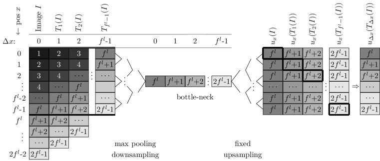
Figure 1: Illustration of a U-Net instance and a 1-dimensional image $I$ such that the functions $\textnormal{u}_{\Delta x}$ are relative-distinct for all $\Delta x$ with $0\leq\Delta x<f^{l}$.

We first define the broad family of U-Net-style encoder-decoder CNNs [22] we consider, followed by a definition of periodic-t shift equivariance. Based on these prerequisites, we prove periodic-$f^{l}$ shift equivariance of U-Nets.

We consider CNNs consisting of $l$ downsampling and $l$ upsampling blocks. A downsampling block consists of a number of conv+nonlinearity layers, followed by max-pooling with downsampling factor (i.e. kernel size and stride) $f$. An upsampling block consists of a number of conv+nonlinearity layers, followed by upsampling by factor $f$, either via nearest-neighbor interpolation (fixed upsampling) or via transposed convolution (learnt upsampling). At each downsampling level of the U-Net, skip connections concatenate the output of the downsampling block before pooling to the input of the respective upsampling block after upsampling, except for the bottom level (also called bottleneck). In the following, we refer to any achitecture of the above family as a U-Net, and to a U-Net with specific weights as a U-Net instance. A U-Net has the capacity to have some property iff there exists an instance of that U-Net with said property. If not noted otherwise, we assume that a U-Net outputs all predictions for an image in one go. Sliding-window / tile-and-stitch mode will be discussed in Section 2.1. Furthermore, if not noted otherwise, we assume valid convolutions in all conv layers. Non-valid padding will be discussed in Section 2.2.

Formally, a U-Net is a function U that maps a discrete, $d$-dimensional input image $I$ with resolution $X_{1}^{in}\times...\times X_{d}^{in}$ and $C^{in}$ channels to an output image with resolution $X_{1}^{out}\times...\times X_{d}^{out}$ and $C^{out}$ channels:

$$\textnormal{U}: \mathbf{R}^{X_{1}^{in}\times..\times X_{d}^{in}\times C^{in}}\!\!\rightarrow\!\mathbf{R}^{X_{1}^{out}\times..\times X_{d}^{out}\times C^{out}}$$ (1)

$$I\mapsto\textnormal{U}(I)\!=\!\left(\textnormal{u}_{\mathbf{x}}(I)\right)_{\mathbf{x}\in X_{1}^{out}\times..\times X_{d}^{out}},$$

where

$$\textnormal{u}_{\mathbf{x}}:\mathbf{R}^{X_{1}^{in}\times...\times X_{d}^{in}\times C^{in}}\rightarrow\mathbf{R}^{C^{out}}\ I\mapsto\textnormal{u}_{\mathbf{x}}(I)=\textnormal{U}(I)(\mathbf{x})$$ (2)

denotes the function that yields the output at output location $\mathbf{x}\in X_{1}^{out}\times...\times X_{d}^{out}$. Concerning functions $\textnormal{u}_{\mathbf{x}}$, two distinct notions of equality can be defined:

Definition 1 (Absolute and Relative Equality).

Two functions $\textnormal{u}_{\mathbf{x}_{1}}$, $\textnormal{u}_{\mathbf{x}_{2}}$ are absolute-equal iff $\forall I:\textnormal{u}_{\mathbf{x}_{1}}(I)=\textnormal{u}_{\mathbf{x_{2}}}(I)$, and absolute-distinct otherwise. Two functions $\textnormal{u}_{\mathbf{x}_{1}}$, $\textnormal{u}_{\mathbf{x}_{2}}$ are relative-equal iff $\forall I:\textnormal{u}_{\mathbf{x}_{1}}(I)=\textnormal{u}_{\mathbf{x}_{2}}(T_{\mathbf{x}_{2}-\mathbf{x}_{1}}(I)),$ with $T_{\Delta\mathbf{x}}(I(\mathbf{x})):=I(\mathbf{x}-\Delta\mathbf{x})$ denoting an image shift by $\Delta\mathbf{x}$. Otherwise $\textnormal{u}_{\mathbf{x}_{1}}$ and $\textnormal{u}_{\mathbf{x}_{2}}$ are relative-distinct.

We provide examples for absolute and relative equality of U-Net functions in Suppl. Sec. 1. Following [28], we define periodic-t shift equivariance as follows:

Definition 2 (Periodic-t Shift Equivariance).

A function F that maps an input image $I$ to an output image $\textnormal{F}(I)$ is periodic-t shift equivariant iff $\textnormal{F}(T_{\Delta\textbf{x}}(I))=T_{\Delta\textbf{x}}(\textnormal{F}(I))$ $\forall\Delta\textbf{x}\in\{(z_{1}\cdot t,...,z_{d}\cdot t)\ |\ z_{i}\in\mathbf{Z}\},$ and $t$ is the smallest number for which this holds.

Lemma 1 (Relative-distinct functions u of a U-Net).

Every U-Net has the capacity to implement $f^{dl}$ relative-distinct functions u, but not more.

Proof 1.

Part I: For any U-Net, we construct an instance and an image $I$ with unique outputs $u_{\textbf{x}-\Delta\textbf{x}}(T_{-\Delta\textbf{x}}(I))$ for all $\Delta\textbf{x}\in\{0,..,f^{l}-1\}^{d}$, proving that every U-Net has the capacity to implement at least $f^{dl}$ relative-distinct functions. Part II: We prove that every U-Net is equivariant to image shifts $f^{l}$, and hence no U-Net has the capacity to implement more than $f^{dl}$ relative-distinct functions.  
Proof part I: We construct a U-Net instance and an input image $I$ which yields $f^{dl}$ relative-distinct output function values, as described in the following. Fig. 1 shows a sketch of our construction for $d=1$. First, for any given U-Net, construct an instance U with fixed upsampling (i.e. all upsampling kernel weights set to 1), all convolutions set to identity, and ignore skip connections by setting respective convolution kernel entries to $0$. For a $d$-dimensional input image I, this U-Net instance yields outputs

$$\textnormal{u}_{\mathbf{x}}(I)=\max\{I(\lfloor\mathbf{x}/f^{l}\rfloor\cdot f^{l}+\Delta\mathbf{x})\ |\ \Delta\mathbf{x}\in\{0,...,f^{l}-1\}^{d}\}.$$

Second, construct a single-channel image $I$ such that $I(\mathbf{x})$ is strictly increasing for increasing positions $\mathbf{x}$ w.r.t. an ordering of positions along diagonals first by the sum of their components and second by their components in increasing order (cf. [5, 23]):

$$\mathbf{x}_{i}>\mathbf{x}_{j}\iff\begin{cases}\sum\limits_{k}x_{i}^{(k)}>\sum\limits_{k}x_{j}^{(k)}&\text{if}\ \sum\limits_{k}x_{i}^{(k)}\neq\sum\limits_{k}x_{j}^{(k)}\\ x_{i}^{(k)}>x_{j}^{(k)}&\text{if}\ \sum\limits_{k}x_{i}^{(k)}=\sum\limits_{k}x_{j}^{(k)}\\ &\text{ and }x_{i}^{(l)}=x_{j}^{(l)}\,\,\forall l<k\end{cases}$$ (3)

For this image, the maximum intensity in any image pixel block of edge length $f^{l}$ is found at the maximum position $(f^{l}-1,...,f^{l}-1)^{d}$. Consequently, as each distinct pixel block of edge length $f^{l}$ covers a unique maximum position,

$$\forall\mathbf{x}\ \forall\Delta\mathbf{x}_{i}\neq\Delta\mathbf{x}_{j}\in \{0,...,f^{l}-1\}^{d}:$$ (4)

$$\textnormal{u}_{\mathbf{x}-\Delta\mathbf{x}_{i}}(T_{-\Delta\mathbf{x}_{i}}(I)) \neq\textnormal{u}_{\mathbf{x}-\Delta\mathbf{x}_{j}}(T_{-\Delta\mathbf{x}_{j}}(I)),$$

i.e. the constructed U-Net instance implements $f^{dl}$ relative-distinct functions u. Proof part II: See Suppl. Sec. 2.

Corollary 1 (Periodic-$f^{l}$ Shift Equivariance of U-Nets).

Every U-Net has the capacity to be periodic-$f^{l}$ shift equivariant.

Proof 2.

Directly follows from the proof of Lemma 1, which shows in Part I that every U-Net has the capacity to be non-equivariant to any shifts $<f^{l}$, and in Part II that every U-Net is shift equivariant to shifts $f^{l}$.

2.1 Tile-and-stitch mode

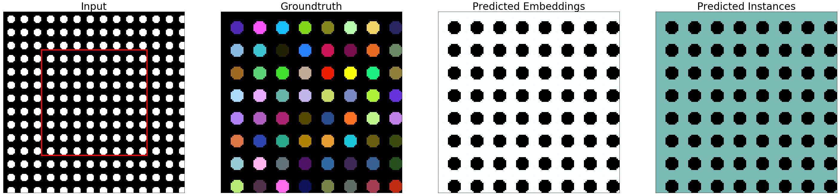
(a) Object spacing $16$ pixels, i.e. a multiple of $f^{l}=8$. Learnt upsampling.

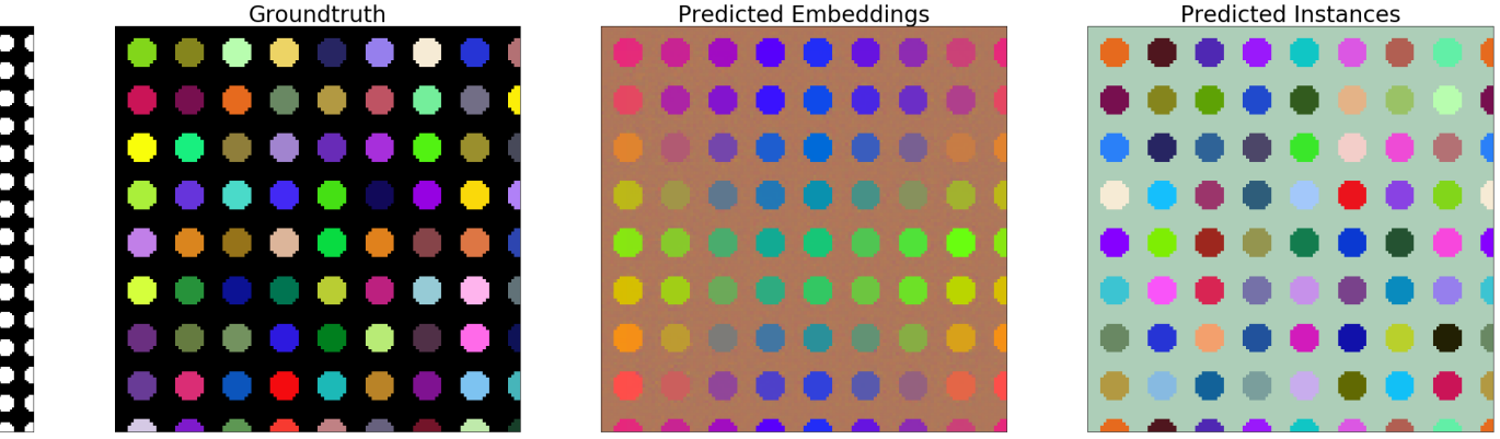
(b) Object spacing $15$ pixels, co-prime with $f^{l}=8$. Learnt upsampling.

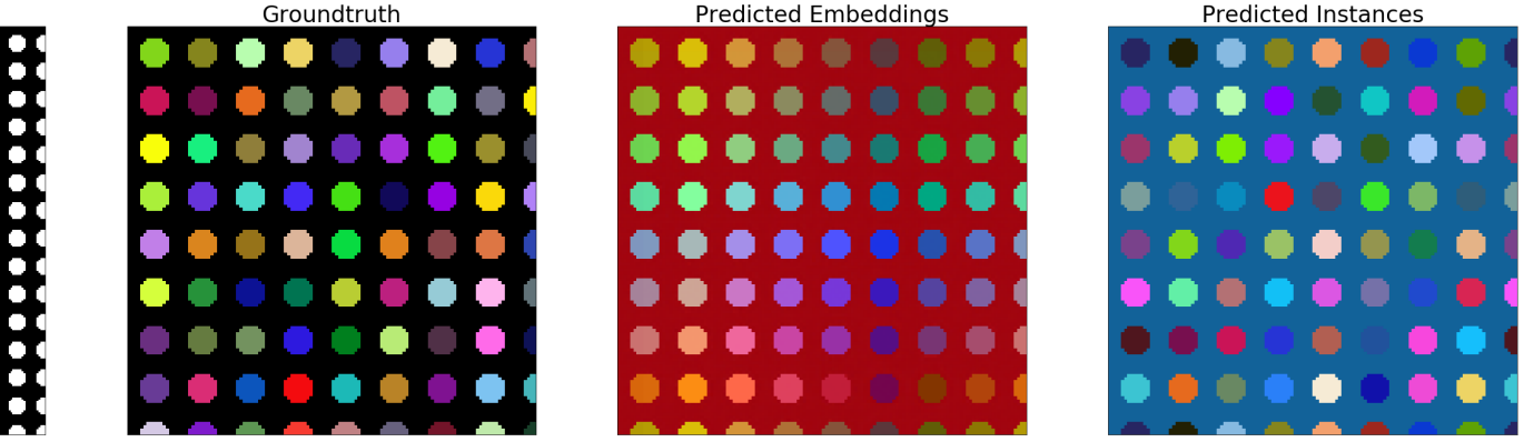
(c) Object spacing $15$ pixels, co-prime with $f^{l}=8$. Fixed upsampling.

Figure 2: A U-Net with $l$ pooling layers and pooling factor $f$ cannot distinguish any instances in an $f^{l}$-periodic $d$-dimensional image of same-looking instances (a). However, it can distinguish up to $f^{d\cdot l}$ instances in a $p$-periodic image of same-looking instances for $p$, $f^{l}$ co-prime (b,c). Showcase: $l=3,f=2,f^{l}=8,f^{dl}=64$. The red box in the input image (top left) shows the valid output window. Analogous results can be achieved for the same object spacings and $l=4,f=2$ (not shown).

In practice, to deal with limited GPU memory, a U-Net is commonly trained on fixed-size input image tiles, yielding fixed-size output tiles. At test time, the output for a full input image is then obtained in a tile-and-stitch manner, where it is common to employ the same tile size as during training, yet larger tile sizes are sometimes employed as inference is less memory-demanding than training.

Concerning shift equivariance in a tile-and-stitch approach with output tile size $w$ during inference, we get (1) periodic-$f^{l}$ shift equivariance within output tiles, and (2) trivially, periodic-$w$ shift equivariance across output tiles. Periodic-$f^{l}$ shift equivariance across the whole output only holds if $w$ is a multiple of $f^{l}$.

2.2 Non-valid padding

The concept of shift equivariance runs counter to the concept of non-valid padding, as the latter does not allow for “clean” input image shifts: Shifting+padding, in general, changes the input image beyond the shift. As a notable consequence, e.g., zero padding renders a CNN with sufficiently large receptive field location-aware [10, 1], thus eviscerating shift equivariance. See [10] for an in-depth discussion of zero-padding and other padding schemes.

3 Analysis of the Impact on Metric Learning for Instance Segmentation

We assess implications of a U-Net’s periodic-$f^{l}$ shift equivariance on the application of instance segmentation via metric learning with discriminative loss [7]. The respective loss function has three terms, a pull-force that pulls pixel embeddings towards their respective instance centroid, a push force that pushes centroids apart, and a penalty on embedding vector lengths. Given predicted embeddings, instances are inferred by mean-shift clustering. For more details, see [7]. First, we assess how many “same-looking” instances a U-Net trained with discriminative loss can distinguish. We call two instances “same-looking” iff the image itself is invariant to shifting by the offset between instance center points. Second, we show the necessity to follow a concise set of simple rules to avoid inconsistencies in a tile-and-stitch approach.

3.1 Distinguishing Same-looking Instances (thus Avoiding False Merges)

Corollary 2.

A U-Net has the capacity to distinguish at most $f^{dl}$ same-looking instances.

Proof 3.

Lemma 1 entails that a U-Net can assign at most $f^{dl}$ different embeddings to a representative pixel of an object instance (say the “central pixel”), namely when positioned at the $f^{dl}$ different relative locations w.r.t. its max-pooling regions. This holds true iff same-looking instances are located at offsets $p$ with $p,f^{l}$ co-prime.

Whether a U-Net is also able to assign same embeddings to all pixels within any instance, thus yielding $f^{dl}$ correct segments, is up to its capacity and the success of training.

Corollary 3.

A U-Net cannot distinguish same-looking instances located at offsets $n\cdot{f^{l}},n\in\mathbf{N}$.

Proof 4.

Periodic-$f^{l}$ shift equivariance of the U-Net entails that it necessarily assigns same embeddings to pixels at same relative locations in the objects.

Fig. 2 showcases Corollaries 2 and 3 on images of periodically arranged disks, for which we trained U-Nets with discriminative loss to predict embeddings $\in\mathbf{R}^{3}$. In particular, it shows that the upper bound of separating $f^{dl}$ same-looking instances, as stated in Corollary 2, can be reached.

3.2 Avoiding False Split Errors in Tile-and-Stitch

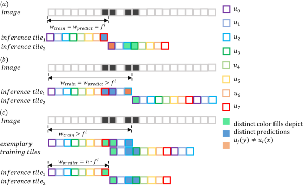
Figure 3: Stitching errors occur when two relative-distinct output functions $u_{i}$ and $u_{j}$ are adjacent to each other during inference, but not during training. Shown here is a 1-d sketch with $l=3$, $f=2$, i.e. with $f^{l}=8$ relative-distinct output functions $u_{i}$, and an exemplary input image containing two instances shown as black filled pixels (where each instance is two pixels wide). In (a) $u_{7}$ is adjacent to $u_{0}$ at the stitching boundary during inference, but during training they were never adjacent due to training output tile size $f^{l}$. This is fixed in (b) where the training output tile size is $>f^{l}$, but during inference $u_{2}$ is adjacent to $u_{0}$ which never occurred during training. In (c) the U-Net was trained as in (b) with training output tile size $>f^{l}$; During inference, however, output tiles are cropped to $n\cdot f^{l}$ to ensure that only functions that were adjacent to each other during training are adjacent at tile boundaries, thus allowing to overcome inconsistencies.

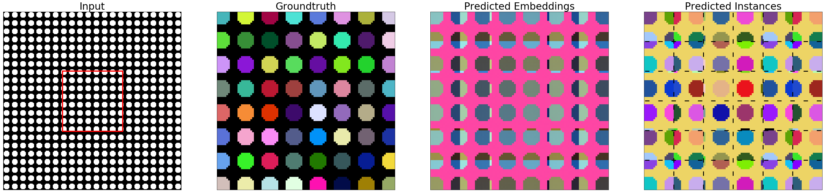
(a) Output tile size $16(=f^{l})$

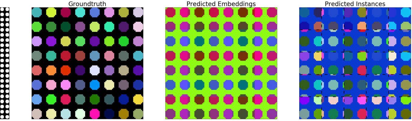
(b) Output tile size $20(>f^{l})$, not cropped before stitching

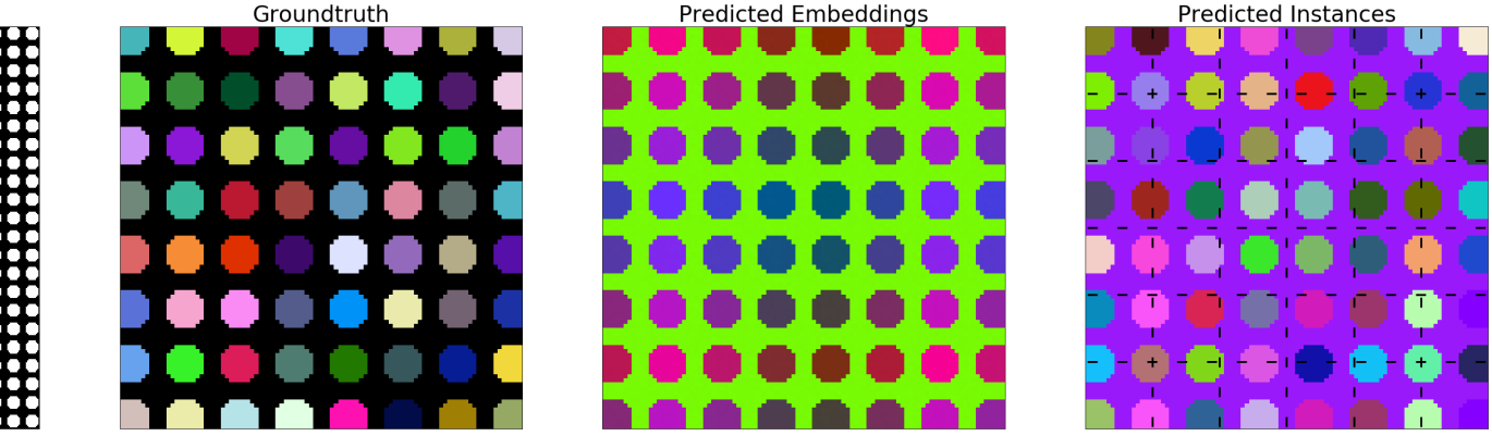
(c) Output tile size cropped to $16(=f^{l})$ before stitching

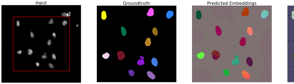
(d) Sample mcf-z-stacks-03212011_f22_s from the BBBC006 cell nuclei dataset [16]

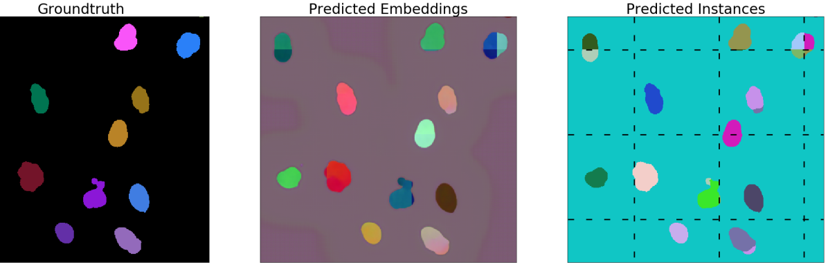
(e) Output tile size $148(>f^{l})$, not cropped before stitching

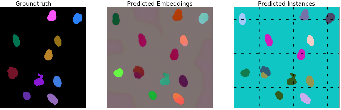
(f) Output tile size cropped to $144(=n\cdot f^{l})$ before stitching

Figure 4: Stitching issues, and how to fix them, for a U-Net with $l=4$ and $f=2$, and a $p$-periodic input image with $p,f^{l}$ co-prime. (a) Training with output window size $w=f^{l}$ yields inconsistencies at $f^{l}$-grid boundaries (black dashed lines) in larger outputs. To avoid inconsistencies, not only is it necessary to (b) train with $w>f^{l}$, which still yields inconsistencies at stitching boundaries when naively stitching $w$-sized tiles, but also to (c) crop tiles to size $n\cdot f^{l}$ before stitching, which solves the issue. (d-f) The same effect occurs on real data: (d) Excerpt from BBBC006 cell nuclei dataset [16]: Naive stitching (e) yields false split errors at tile boundaries, while correct stitching (f) fixes them. (See Suppl. Fig. 1 for resp. embeddings.) Note that slight differences between (e) and (f) within tiles occur because predictions stem from different U-Net output functions.

In the following, we analyze the impact of output tile size on training with discriminative loss, as well as on inference in a tile-and-stitch manner. To this end, we assess which of the $f^{dl}$ potentially relative-distinct output functions of a U-Net contribute to the loss, and which pairs of functions that predict directly neighboring outputs in a stitched solution contribute to an instance’s pull force loss term during training. Fig. 3 exemplifies our analysis on a 1-d input image that contains a couple of two-pixel-wide instances.

Training output tile size $<f^{l}$: In this case, some of the $f^{dl}$ output functions of the U-Net never contribute to the loss, i.e. they are not explicitly trained. In effect, they may yield nonsensical predictions when used during inference.

Training output tile size $=f^{l}$: In this case, all output functions of the U-Net are considered during training in each batch. However, some pairs of functions that predict neighboring outputs during inference are never considered as neighbors during training. E.g. for $d=1$, $\textnormal{u}_{0}$ and $\textnormal{u}_{f^{l}-1}$ never predict directly neighboring embeddings during training, and hence never contribute to the pull force loss term as direct neighbors. They do, however, predict directly neighboring embeddings during inference, no matter if stitching $f^{l}$-sized output tiles or employing larger output tiles (potentially alleviating the need for stitching) during inference. Consequently, in this case, embeddings predicted at neighboring pixels at $f^{l}$-grid-boundaries may be inconsistent.

Training output tile size $>\!f^{l}$: All possible direct neighborhoods of output functions are considered during training, given that inference output tile size is a multiple of $f^{l}$.

Inference output tile size $\neq n\cdot f^{l}$: Similar to the case of training output tile size $=f^{l}$, functions that predict neighboring outputs on two sides of a stitching boundary have never contributed to the same pull force term as neighbors during training (assuming batch size 1). Consequently, inconsistencies may occur at stitching boundaries.

Inference output tile size $=n\cdot f^{l}$: Tile-and-stitch processing is guaranteed to not be causal for any inconsistencies, as formalized by the following Corollary:

Corollary 4.

If valid padding and output tiles of size $n\cdot f^{l}$ are employed, tile-and-stitch is equivalent to processing whole images at once.

Proof 5.

This directly follows from identical arrangements of respective output functions, namely arrangement into a regular grid of d-dimensional blocks of size $f^{dl}$.

Zero padding:

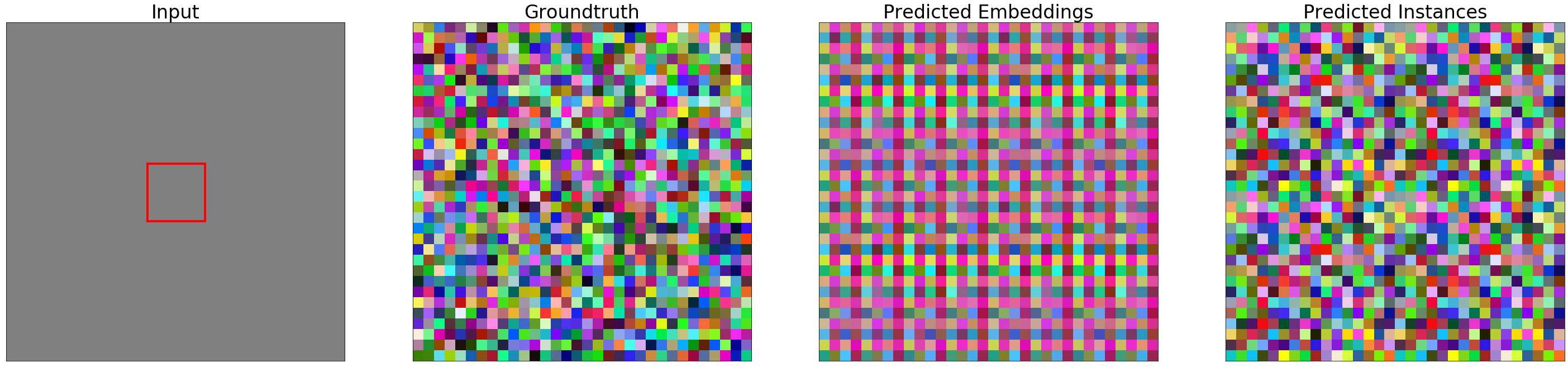
Figure 5: A U-Net with valid padding and learnt upsampling can learn to assign a unique ID to each pixel in an output window of size $f^{l}$, independent of the input image. This is not possible with nearest-neighbor upsampling. Showcase: $l=4,f=2$, input image $I\equiv 1$. Output: repeating pattern of $f^{dl}=256$ unique IDs.

A U-Net with zero padding, training output window size $w$, and sufficiently large receptive field implements up to $w^{d}$ relative-distinct functions [10]. Assuming batch size 1, this yields inconsistencies at stitching boundaries analogous to the valid-padding cases discussed above. Related work has attributed this effect to zero padding [9, 21], yet to our knowledge, mitigation has been limited to using larger tiles during inference [9, 21]. Valid padding has been investigated as a potential remedy [21], yet to no avail due to a lack of formal analysis.

Necessary rules to avoid inconsistencies at stitching boundaries: Following from the above considerations, in general, to avoid inconsistencies in a tile-and-stitch approach, at training time, assuming standard batch size 1 and valid convolutions, it is necessary to train with output window size $>f^{l}$. Furthermore, at test time, it is necessary to crop output tiles of size $\neq n\cdot f^{l}$ to some $n\cdot f^{l}$ before stitching ($n\geq 1$). Fig. 4(a)-4(c) showcases the necessity of following the rules on synthetic images of periodically arranged disks.

For the case of zero padding, training with batch size $>1$ is necessary to avoid inconsistencies, where training output tiles in a batch have to be directly neighboring. Note, however, that batch size $>1$ is uncommon due to GPU memory limitations, and hence may entail further architectural changes to be feasible.

3.3 Location awareness

Corollary 5.

A U-Net with valid padding and learnt upsampling has the capacity to assign a unique ID to each pixel in an output window of size $f^{dl}$, independent of the specific input image.

Proof 6.

Proof by construction: Set the first convolution to weights zero and bias 1. This yields a constant feature map. Set all other convolutions to identity. Thus, a feature map in the bottleneck layer will be constant. Ignore skip connections by setting respective convolution kernel entries to zero. Construct upsampling filter kernels $p_{1}\dots p_{l}$ by filling them with non-repeating prime numbers. For this, $l\cdot f^{d}$ prime numbers are needed. Each of the $f^{dl}$ output functions $u_{i}$ of this U-Net instance yields a product over a unique set of $l$ distinct prime numbers. As the decomposition of any number into prime factors is unique, respective outputs effectively assign a unique ID to each output pixel.

Fig. 5 showcases the level of location awareness that can be reached with a U-Net with valid padding and learnt upsampling, trained via metric learning with discriminative loss [7] to segment pixels as individual instances given a constant input image. This confirms that a U-Net instance akin to the construction in Proof 6 can be trained. A comparable effect of location awareness, albeit with conceptually different cause, has been described for zero-padding [10], which we showcase in Suppl. Fig. 2

Assigning unique IDs to pixels is yet another example of reaching the upper bound of distinguishing $f^{dl}$ instances (cf. Fig. 2), namely for the extreme case that each pixel in a constant input image forms an individual instance. However, this can only be achieved with learnt upsampling, or non-valid padding (cf. [10]). This is because for valid padding and fixed upsampling, a constant input image is always mapped to a constant output image.

To our knowledge, our work is first to report location awareness given valid padding, thereby raising the question whether approaches that explicitly consider pixel locations or some other form of pixel IDs as additional inputs might be obsolete in case of valid padding and learnt upsampling.

4 Practical Impact

We empirically assessed the practical impact of periodic-t shift equivariance on instance segmentation on synthetic images with added noise and deformations (Sec. 4.1), as well as on benchmark data (Sec. 4.2).

4.1 Noise and Small Deformations

A U-Net with $l$ levels and pooling factor $f$ fails to discriminate any instances in an infinite image of periodic-$f^{l}$ arranged objects (cf. Fig. 2(a)). However we showcase in Suppl. Figs. 3a, 3b that it may suffice to add slight Gaussian noise or small random elastic deformations to the input image to “fix” the shift equivariance problem. Here, we generate noise or deformations randomly, on-the-fly per training step as well as at test time. Hence the observed effect is not due to over-fitting to a particular noisy/deformed image.

However, note that neither noise nor elastic deformations do anything to fix the issue of inconsistencies in a tile-and-stitch approach if stitching is not performed according to the rules derived in Sec. 3.2, as illustrated in Suppl. Figs. 3c, 3d.

4.2 Quantitative Evaluation on Benchmark Data

Avoiding False Splits: We assessed the practical impact of correct tile-and-stitch on avoiding false split errors on three cell nuclei segmentation datasets, namely BBBC006 [16], DSB2018 [26, 4], and nuclei3d [8, 17] (see Suppl. Sec. 3 for details). We assessed AP 0.5, as well as false split- and false merge errors as defined in [3]. We performed tile-and-stitch with a range of output window sizes. Correct tile-and-stitch, i.e. with output window size $n\cdot f^{l}$, drastically reduces false splits and increases AP 0.5 accordingly, as plotted in Fig. 6, and exemplified in Fig. 4(d)-4(f) and Suppl. Fig. 1.

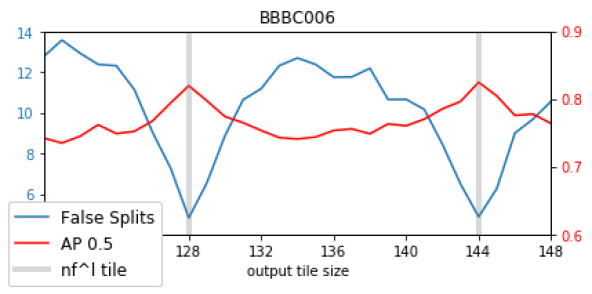
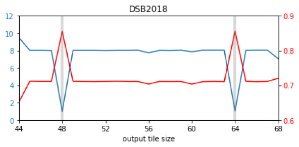
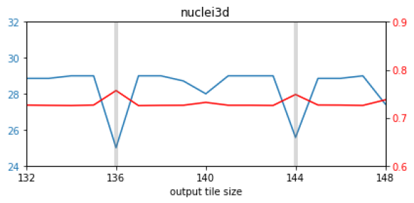
Figure 6: Output tile size vs. false splits and AP 0.5 on three cell nuclei datasets, covering 2d and 3d image data. 2d: Left: BBBC006 [16], middle: the DSB2018 [26] subset of BBBC038v1 [4]. 3d: Right: nuclei3d [8, 17]

Distinguishing Instances: We assessed the practical impact of periodic-$f^{l}$ shift equivariance on distinguishing instances on BBBC006. If periodic-$f^{l}$ shift equivariance were of practical impact here, we would (1) expect to see false merge errors of distant, i.e. non-touching, objects (whereas touching objects may be merged for other, confounding reasons), and (2) we would expect distant false merges to occur for similar-looking objects. On average, for 97.3 instances per test image, 3.8 false merge errors occur, and merged instances do not look similar by eye, as exemplified in Fig. 7. This empirical study cannot prove that periodic-$f^{l}$ shift equivariance is not of practical impact on distinguishing instances – this would only follow if there were no false merges, which is unlikely due to chance alone. However, it does suggest that the impact is negligible.

Figure 7: Exemplary distant-merged objects do not look alike in raw images (excerpts from BBBC006 [16]), making periodic-$f^{l}$ shift equivariance an unlikely culprit.

5 Discussion and Conclusion

Our work provides a formal analysis of the impact of shift equivariance properties of common encoder-decoder style CNNs on the task of metric learning for instance segmentation. Contrary to a range of works that have dismissed it as fundamentally flawed due to the assumed shift equivariance of CNNs, our theoretical analysis reveals the precise shift equivariance properties of U-Net style CNNs, from which follows that a U-Net with $l$ levels and downsampling factor $f$ is indeed able to distinguish up to $f^{dl}$ identical-looking (in terms of their respective receptive fields) instances in a $d$-dimensional image, given that object spacing is co-prime to $f^{l}$ in any dimension. In particular, our work refutes some findings of Novotny et al. [19] on similar synthetic imagery of periodically arranged discs (cf. their Fig. 3c in [19]): They attribute the observed “near-random”, noise-like patterns within instances to the assumed ill-suitedness of metric learning for the task of instance segmentation, whereas our results on comparable data exhibit clean clusters in all cases (cf. our Fig. 2). As for differences in our model and theirs, they omit the push force in their “simplified” discriminative loss, while we employ it, thus avoiding that constant embeddings across all instances constitute a global optimum. Furthermore, they employ k-means clustering with k the correct number of instances, while we employ mean shift clustering, thus avoiding that clustering results are ill-defined in case of constant embeddings across instances (cf. our Fig. 2(a)). Concerning the specific patterns within the disks in their Fig. 3c, a shift equivariant CNN would necessarily yield identical patterns for identical instances. Instead, the figure shows multiple periodically alternating distinct patterns within instances, which violates their general assumption of shift equivariance, but is consistent with our theory, given that their truncated ResNet50 architecture is periodic-4 shift equivariant as it employs one max pooling layer with $f\!=\!2$ and one convolutional layer with stride 2 (where stride works analogous to pooling in terms of its effect on shift equivariance).

Beyond our formal analysis of shift equivariance properties, we show empirically on synthetic data that adding barely visible amounts of noise or elastic deformation can enable a U-Net to distinguish objects even at ”unfortunate” object spacing $f^{l}$. Furthermore, we show on real data that, while distant objects are falsely merged sporadically, this cannot straightforwardly be attributed to shift equivariance, as we do not find respective merged instances to look similar by visual inspection.

We deem of even greater impact to practitioners our theoretical analysis of inconsistencies that have been reported when performing metric learning with discriminative loss for instance segmentation in a tile-and-stitch approach due to large, GPU-memory-busting inputs. To this end, our theoretical analysis of shift equivariance allows us to derive a simple set of rules that necessarily have to be followed to avoid inconsistencies at stitching boundaries when performing inference on large data. While our impact analysis in this work is tailored to metric learning with discriminative loss, the same theory of shift equivariance yields similar implications for other pixel-wise prediction tasks for which tile-and-stitch issues with inconsistencies have been reported, like semantic segmentation (as e.g. studied empirically in [21]) or image registration. In particular, the proven equivalence between whole-image prediction and tile-and-stitch prediction with output tile size $n\cdot f^{l}$ holds independent of the specific training task.
Acknowledgements. We wish to thank Anna Kreshuk and Fred Hamprecht for inspiring discussions. Funding: J.L.R.: German Research Foundation RTG 2424. J.L.R, M.D., P.H., L.M., A.M. and D.K.: Berlin Institute of Health and Max-Delbrueck-Center for Molecular Medicine in the Helmholtz Association (MDC). P.H.: MDC-NYU exchange program and HFSP grant RGP0021/2018-102. X.Y.: Helmholtz Einstein International Berlin Research School in Data Science. V.E.G.: German Research Foundation CRC 1404. J.F.: HHMI. P.H., L.M. and D.K. were supported by the HHMI Janelia Visiting Scientist Program.

References

- [1] Bilal Alsallakh, Narine Kokhlikyan, Vivek Miglani, Jun Yuan, and Orion Reblitz-Richardson. Mind the Pad–CNNs can Develop Blind Spots. arXiv preprint arXiv:2010.02178, 2020.
- [2] Aharon Azulay and Yair Weiss. Why do deep convolutional networks generalize so poorly to small image transformations? arXiv preprint arXiv:1805.12177, 2018.
- [3] Juan C Caicedo et al. Evaluation of deep learning strategies for nucleus segmentation in fluorescence images. Cytometry Part A, 95(9):952–965, 2019.
- [4] Juan C. Caicedo, Allen Goodman, Kyle W. Karhohs, Beth A. Cimini, Jeanelle Ackerman, Marzieh Haghighi, CherKeng Heng, Tim Becker, Minh Doan, Claire McQuin, Mohammad Rohban, Shantanu Singh, and Anne E. Carpenter. Nucleus segmentation across imaging experiments: the 2018 Data Science Bowl. Nature Methods, 16(12):1247–1253, Dec 2019.
- [5] G. Cantor. Ein Beitrag zur Mannigfaltigkeitslehre. Journal für die reine und angewandte Mathematik, 84:242–258, 1877.
- [6] Long Chen, Martin Strauch, and Dorit Merhof. Instance Segmentation of Biomedical Images with an Object-Aware Embedding Learned with Local Constraints. In International Conference on Medical Image Computing and Computer-Assisted Intervention, pages 451–459. Springer, 2019.
- [7] Bert De Brabandere, Davy Neven, and Luc Van Gool. Semantic instance segmentation with a discriminative loss function. arXiv preprint arXiv:1708.02551, 2017.
- [8] Peter Hirsch and Dagmar Kainmueller. An auxiliary task for learning nuclei segmentation in 3d microscopy images. In Medical Imaging with Deep Learning, pages 304–321. PMLR, 2020.
- [9] Bohao Huang, Daniel Reichman, Leslie M Collins, Kyle Bradbury, and Jordan M Malof. Tiling and Stitching Segmentation Output for Remote Sensing: Basic Challenges and Recommendations. arXiv preprint arXiv:1805.12219, 2018.
- [10] Osman Semih Kayhan and Jan C. van Gemert. On translation invariance in CNNs: Convolutional layers can exploit absolute spatial location. In Proceedings of the IEEE/CVF Conference on Computer Vision and Pattern Recognition, pages 14274–14285, 2020.
- [11] Victor Kulikov and Victor Lempitsky. Instance segmentation of biological images using harmonic embeddings. In Proceedings of the IEEE/CVF Conference on Computer Vision and Pattern Recognition, pages 3843–3851, 2020.
- [12] Victor Kulikov, Victor Yurchenko, and Victor Lempitsky. Instance segmentation by deep coloring. arXiv preprint arXiv:1807.10007, 2018.
- [13] Kisuk Lee, Ran Lu, Kyle Luther, and H Sebastian Seung. Learning dense voxel embeddings for 3d neuron reconstruction. arXiv preprint arXiv:1909.09872, 2019.
- [14] Kisuk Lee, Jonathan Zung, Peter Li, Viren Jain, and H Sebastian Seung. Superhuman accuracy on the SNEMI3D connectomics challenge. arXiv preprint arXiv:1706.00120, 2017.
- [15] Rosanne Liu, Joel Lehman, Piero Molino, Felipe Petroski Such, Eric Frank, Alex Sergeev, and Jason Yosinski. An intriguing failing of convolutional neural networks and the coordconv solution. Advances in Neural Information Processing Systems, 31:9605–9616, 2018.
- [16] Vebjorn Ljosa, Katherine L Sokolnicki, and Anne E Carpenter. Annotated high-throughput microscopy image sets for validation. Nature methods, 9(7):637–637, 2012.
- [17] Fuhui Long, Hanchuan Peng, Xiao Liu, Stuart K Kim, and Eugene Myers. A 3D digital atlas of C. elegans and its application to single-cell analyses. Nature methods, 6(9):667, 2009.
- [18] Davy Neven, Bert De Brabandere, Marc Proesmans, and Luc Van Gool. Instance segmentation by jointly optimizing spatial embeddings and clustering bandwidth. In Proceedings of the IEEE/CVF Conference on Computer Vision and Pattern Recognition, pages 8837–8845, 2019.
- [19] David Novotny, Samuel Albanie, Diane Larlus, and Andrea Vedaldi. Semi-convolutional operators for instance segmentation. In Proceedings of the European Conference on Computer Vision, pages 86–102, 2018.
- [20] Augustus Odena, Vincent Dumoulin, and Chris Olah. Deconvolution and checkerboard artifacts. Distill, 1(10):e3, 2016.
- [21] G Anthony Reina, Ravi Panchumarthy, Siddhesh Pravin Thakur, Alexei Bastidas, and Spyridon Bakas. Systematic Evaluation of Image Tiling Adverse Effects on Deep Learning Semantic Segmentation. Frontiers in Neuroscience, 14:65, 2020.
- [22] Olaf Ronneberger, Philipp Fischer, and Thomas Brox. U-net: Convolutional networks for biomedical image segmentation. In International Conference on Medical Image Computing and Computer-Assisted Intervention, pages 234–241. Springer, 2015.
- [23] Arnold L. Rosenberg. Efficient pairing functions - and why you should care. International Journal of Foundations of Computer Science, 14(01):3–17, 2003.
- [24] Josef Lorenz Rumberger, Lisa Mais, and Dagmar Kainmueller. Probabilistic deep learning for instance segmentation. arXiv preprint arXiv:2008.10678, 2020.
- [25] Dominik Scherer, Andreas Müller, and Sven Behnke. Evaluation of pooling operations in convolutional architectures for object recognition. In International Conference on Artificial Neural Networks, pages 92–101. Springer, 2010.
- [26] Uwe Schmidt, Martin Weigert, Coleman Broaddus, and Gene Myers. Cell Detection with Star-Convex Polygons. Lecture Notes in Computer Science, 2018.
- [27] Carsen Stringer, Michalis Michaelos, and Marius Pachitariu. Cellpose: a generalist algorithm for cellular segmentation. bioRxiv, 2020.
- [28] Richard Zhang. Making convolutional networks shift-invariant again. arXiv preprint arXiv:1904.11486, 2019.