Scaling the Convex Barrier with Sparse Dual Algorithms

Abstract

Tight and efficient neural network bounding is crucial to the scaling of neural network verification systems. Many efficient bounding algorithms have been presented recently, but they are often too loose to verify more challenging properties. This is due to the weakness of the employed relaxation, which is usually a linear program of size linear in the number of neurons. While a tighter linear relaxation for piecewise-linear activations exists, it comes at the cost of exponentially many constraints and currently lacks an efficient customized solver. We alleviate this deficiency by presenting two novel dual algorithms: one operates a subgradient method on a small active set of dual variables, the other exploits the sparsity of Frank-Wolfe type optimizers to incur only a linear memory cost. Both methods recover the strengths of the new relaxation: tightness and a linear separation oracle. At the same time, they share the benefits of previous dual approaches for weaker relaxations: massive parallelism, GPU implementation, low cost per iteration and valid bounds at any time. As a consequence, we can obtain better bounds than off-the-shelf solvers in only a fraction of their running time, attaining significant formal verification speed-ups.

Keywords: Neural Network Verification, Neural Network Bounding, Dual Algorithms, Convex Optimization, Branch and Bound

1 Introduction

Verification requires formally proving or disproving that a given property of a neural network holds over all inputs in a specified domain. We consider properties in their canonical form (Bunel et al., 2018), which requires us to either: (i) prove that no input results in a negative output (property is true); or (ii) identify a counter-example (property is false). The search for counter-examples is typically performed by efficient methods such as random sampling of the input domain (Webb et al., 2019), or projected gradient descent (Kurakin et al., 2017; Carlini and Wagner, 2017; Madry et al., 2018). In contrast, establishing the veracity of a property requires solving a suitable convex relaxation to obtain a lower bound on the minimum output. If the lower bound is positive, the given property is true. If the bound is negative and no counter-example is found, either: (i) we make no conclusions regarding the property (incomplete verification); or (ii) we further refine the counter-example search and lower bound computation within a branch-and-bound framework until we reach a concrete conclusion (complete verification).

The main bottleneck of branch and bound is the computation of the lower bound for each node of the enumeration tree via convex optimization. While earlier works relied on off-the-shelf solvers (Ehlers, 2017; Bunel et al., 2018), it was quickly established that such an approach does not scale-up elegantly with the size of the neural network. This has motivated researchers to design specialized dual solvers (Dvijotham et al., 2019; Bunel et al., 2020a), thereby providing initial evidence that verification can be realised in practice. However, the convex relaxation considered in the dual solvers is itself very weak (Ehlers, 2017), hitting what is now commonly referred to as the “convex barrier” (Salman et al., 2019). In practice, this implies that either several properties remain undecided in incomplete verification, or take several hours to be verified exactly.

Multiple works have tried to overcome the convex barrier for piecewise linear activations (Raghunathan et al., 2018; Singh et al., 2019a). Here, we focus on the single-neuron Linear Programming (LP) relaxation by Anderson et al. (2020). Unfortunately, its tightness comes at the price of exponentially many (in the number of variables) constraints. Therefore, existing dual solvers (Dvijotham et al., 2018; Bunel et al., 2020a) are not easily applicable, limiting the scaling of the new relaxation.

We address this problem by presenting two specialized dual solvers for the relaxation by Anderson et al. (2020), which realize its full potential by meeting the following desiderata:

• Relying on an active set of dual variables, we present a unified dual treatment that includes both a linearly sized LP relaxation (Ehlers, 2017) and the tighter formulation. As a consequence, we obtain an inexpensive dual initializer, named Big-M, which is competitive with dual approaches on the looser relaxation (Dvijotham et al., 2018; Bunel et al., 2020a). Moreover, by dynamically extending the active set, we obtain a subgradient-based solver, named Active Set, which rapidly overcomes the convex barrier and yields much tighter bounds if a larger computational budget is available.

• The tightness of the bounds attainable by Active Set depends on the memory footprint through the size of the active set. By exploiting the properties of Frank-Wolfe style optimizers (Frank and Wolfe, 1956), we present Saddle Point, a solver that deals with the exponentially many constraints of the relaxation by Anderson et al. (2020) while only incurring a linear memory cost. Saddle Point eliminates the dependency on memory at the cost of a potential reduction of the dual feasible space, but is nevertheless very competitive with Active Set in settings requiring tight bounds.

• Both solvers are sparse and recover the strengths of the original primal problem (Anderson et al., 2020) in the dual domain. In line with previous dual solvers, both methods yield valid bounds at anytime, leverage convolutional network structure and enjoy massive parallelism within a GPU implementation, resulting in better bounds in an order of magnitude less time than off-the-shelf solvers (Gurobi Optimization, 2020). Owing to this, we show that both solvers can yield large complete verification gains compared to primal approaches (Anderson et al., 2020) and previous dual algorithms.

A preliminary version of this work appeared in the proceedings of the Ninth International Conference on Learning Representations (De Palma et al., 2021). The present article significantly extends it by:

1. Presenting Saddle Point ($\S$5), a second solver for the relaxation by Anderson et al. (2020), which is more memory efficient than both Active Set and the original cutting plane algorithm by Anderson et al. (2020).

2. Providing a detailed experimental evaluation of the new solver, both for incomplete and complete verification.

3. Presenting an adaptive and more intuitive scheme to switch from looser to tighter bounding algorithms within branch and bound ($\S$6.2).

4. Investigating the effect of different speed-accuracy trade-offs from the presented solvers in the context of complete verification ($\S$8.3.2).

2 Preliminaries: Neural Network Relaxations

We denote vectors by bold lower case letters (for example, $\mathbf{x}$) and matrices by upper case letters (for example, $W$). We use $\odot$ for the Hadamard product, $\llbracket\cdot\rrbracket$ for integer ranges, $\mathds{1}_{{\mathbf{a}}}$ for the indicator vector on condition $\mathbf{a}$ and brackets for intervals ($[\mathbf{l}_{k},\mathbf{u}_{k}]$) and vector or matrix entries ($\mathbf{x}[i]$ or $W[i,j]$). In addition, $\text{col}_{i}(W)$ and $\text{row}_{i}(W)$ respectively denote the $i$-th column and the $i$-th row of matrix $W$. Finally, given $W\in\mathbb{R}^{m\times n}$ and $\mathbf{x}\in\mathbb{R}^{m}$, we will employ $W\diamond\mathbf{x}$ and $W\oblong\mathbf{x}$ as shorthands for respectively $\sum_{i}\text{col}_{i}(W)\odot\mathbf{x}$ and $\sum_{i}\text{col}_{i}(W)^{T}\mathbf{x}$.

Let $\mathcal{C}$ be the network input domain. Similar to Dvijotham et al. (2018); Bunel et al. (2020a), we assume that the minimization of a linear function over $\mathcal{C}$ can be performed efficiently. Our goal is to compute bounds on the scalar output of a piecewise-linear feedforward neural network. The tightest possible lower bound can be obtained by solving the following optimization problem:

$$\smash{\min_{\mathbf{x},\mathbf{\hat{x}}}}\quad\hat{x}_{n}\qquad\text{s.t. }\quad \mathbf{x}_{0}\in\mathcal{C},$$ (1a)

$$\mathbf{\hat{x}}_{k+1}=W_{k+1}\mathbf{x}_{k}+\mathbf{b}_{k+1}\quad k\in\left\llbracket 0,n-1\right\rrbracket,$$ (1b)

$$\mathbf{x}_{k}=\sigma\left(\mathbf{\hat{x}}_{k}\right)\quad k\in\left\llbracket 1,n-1\right\rrbracket,$$ (1c)

where the activation function $\sigma\left(\mathbf{\hat{x}}_{k}\right)$ is piecewise-linear, $\mathbf{\hat{x}}_{k},\mathbf{x}_{k}\in\mathbb{R}^{n_{k}}$ denote the outputs of the $k$-th linear layer (fully-connected or convolutional) and activation function respectively, $W_{k}$ and $\mathbf{b}_{k}$ denote its weight matrix and bias, $n_{k}$ is the number of activations at layer k. We will focus on the ReLU case ($\sigma\left(\mathbf{x}\right)=\max\left(\mathbf{x},0\right)$), as common piecewise-linear functions can be expressed as a composition of ReLUs (Bunel et al., 2020b).

Problem (1) is non-convex due to the activation function’s non-linearity, that is, due to constraint (1c). As solving it is NP-hard (Katz et al., 2017), it is commonly approximated by a convex relaxation (see $\S$7). The quality of the corresponding bounds, which is fundamental in verification, depends on the tightness of the relaxation. Unfortunately, tight relaxations usually correspond to slower bounding procedures. We first review a popular ReLU relaxation in $\S$2.1. We then consider a tighter one in $\S$2.2.

2.1 Planet Relaxation

The so-called Planet relaxation (Ehlers, 2017) has enjoyed widespread use due to its amenability to efficient customised solvers (Dvijotham et al., 2018; Bunel et al., 2020a) and is the “relaxation of choice” for many works in the area (Salman et al., 2019; Singh et al., 2019b; Bunel et al., 2020b; Balunovic and Vechev, 2020; Lu and Kumar, 2020). Here, we describe it in its non-projected form $\mathcal{M}_{k}$, corresponding to the LP relaxation of the Big-M Mixed Integer Programming (MIP) formulation (Tjeng et al., 2019). Applying $\mathcal{M}_{k}$ to problem (1) results in the following linear program:

$$\smash{\min_{\mathbf{x},\mathbf{\hat{x}},\mathbf{z}}}\quad\hat{x}_{n}\quad\text{s.t. } \mathbf{x}_{0}\in\mathcal{C}\hfil\hfil$$ (2)

$$\mathbf{\hat{x}}_{k+1}=W_{k+1}\mathbf{x}_{k}+\mathbf{b}_{k+1} k\in\left\llbracket 0,n-1\right\rrbracket,$$

$$\left.\begin{array}[]{l}\mathbf{x}_{k}\geq\mathbf{\hat{x}}_{k},\quad\mathbf{x}_{k}\leq\hat{\mathbf{u}}_{k}\odot\mathbf{z}_{k},\\ \mathbf{x}_{k}\leq\mathbf{\hat{x}}_{k}-\hat{\mathbf{l}}_{k}\odot(1-\mathbf{z}_{k}),\\ (\mathbf{x}_{k},\mathbf{\hat{x}}_{k},\mathbf{z}_{k})\in[\mathbf{l}_{k},\mathbf{u}_{k}]\times[\hat{\mathbf{l}}_{k},\hat{\mathbf{u}}_{k}]\times[\mathbf{0},\ \mathbf{1}]\end{array}\right\}:=\mathcal{M}_{k} k\in\left\llbracket 1,n-1\right\rrbracket,$$

where $\hat{\mathbf{l}}_{k},\hat{\mathbf{u}}_{k}$ and $\mathbf{l}_{k},\mathbf{u}_{k}$ are intermediate bounds respectively on pre-activation variables $\mathbf{\hat{x}}_{k}$ and post-activation variables $\mathbf{x}_{k}$. These constants play an important role in the structure of $\mathcal{M}_{k}$ and, together with the relaxed binary constraints on $\mathbf{z}$, define box constraints on the variables. We detail how to compute intermediate bounds in appendix E. Projecting out auxiliary variables $\mathbf{z}$ results in the Planet relaxation (cf. appendix B.1 for details), which replaces (1c) by its convex hull.

Problem (2), which is linearly-sized, can be easily solved via commercial black-box LP solvers (Bunel et al., 2018). This does not scale-up well with the size of the neural network, motivating the need for specialized solvers. Customised dual solvers have been designed by relaxing constraints (1b), (1c) (Dvijotham et al., 2018) or replacing (1c) by the Planet relaxation and employing Lagrangian Decomposition (Bunel et al., 2020a). Both approaches result in bounds very close to optimality for problem (2) in only a fraction of the runtime of off-the-shelf solvers.

2.2 A Tighter Relaxation

A much tighter approximation of problem (1) than the Planet relaxation ($\S$2.1) can be obtained by representing the convex hull of the composition of constraints (1b) and (1c) rather than the convex hull of constraint (1c) alone. A formulation of this type was recently introduced by Anderson et al. (2020).

Let us define $\smash{\check{L}_{k-1},\check{U}_{k-1}\in\mathbb{R}^{n_{k}\times n_{k-1}}}$ as:

$$\check{L}_{k-1}[i,j] =\mathbf{l}_{k-1}[j]\mathds{1}_{W_{k}[i,j]\geq 0}+\mathbf{u}_{k-1}[j]\mathds{1}_{W_{k}[i,j]<0},$$

$$\check{U}_{k-1}[i,j] =\mathbf{u}_{k-1}[j]\mathds{1}_{W_{k}[i,j]\geq 0}+\mathbf{l}_{k-1}[j]\mathds{1}_{W_{k}[i,j]<0}.$$

Additionally, let us introduce $\smash{2^{W_{k}}=\{0,1\}^{n_{k}\times n_{k-1}}}$, the set of all possible binary masks of weight matrix $W_{k}$, and $\mathcal{E}_{k}:=2^{W_{k}}\setminus\{0,1\}$, which excludes the all-zero and all-one masks. The new representation results in the following primal problem:

$$\begin{aligned} \min_{\mathbf{x},\mathbf{\hat{x}},\mathbf{z}}\ \hat{x}_{n}\enskip\text{s.t. }\enskip&\mathbf{x}_{0}\in\mathcal{C}\hfil\hfil\displaystyle\\[-7.0pt] &\mathbf{\hat{x}}_{k+1}=W_{k+1}\mathbf{x}_{k}+\mathbf{b}_{k+1}&&k\in\left\llbracket 0,n-1\right\rrbracket,\\ &\left.\begin{array}[]{l}(\mathbf{x}_{k},\mathbf{\hat{x}}_{k},\mathbf{z}_{k})\in\mathcal{M}_{k}\\ \mathbf{x}_{k}\leq\left(\begin{array}[]{l}\left(W_{k}\odot I_{k}\right)\mathbf{x}_{k-1}+\mathbf{z}_{k}\odot\mathbf{b}_{k}\\ -\left(W_{k}\odot I_{k}\odot\check{L}_{k-1}\right)\diamond(1-\mathbf{z}_{k})\\ +\left(W_{k}\odot\left(1-I_{k}\right)\odot\check{U}_{k-1}\right)\diamond\mathbf{z}_{k}\end{array}\right)\ \forall I_{k}\in\mathcal{E}_{k}\end{array}\right\}:=\mathcal{A}_{k}&&k\in\left\llbracket 1,n-1\right\rrbracket.\end{aligned}$$ (3)

Both $\mathcal{M}_{k}$ and $\mathcal{A}_{k}$ yield valid MIP formulations for problem (1) when imposing integrality constraints on $\mathbf{z}$. However, the LP relaxation of $\mathcal{A}_{k}$ will yield tighter bounds. In the worst case, this tightness comes at the cost of exponentially many constraints: one for each $I_{k}\in{\cal E}_{k}$. On the other hand, given a set of primal assignments $(\mathbf{x},\mathbf{z})$ that are not necessarily feasible for problem (3), one can efficiently compute the most violated constraint (if any) at that point. Denoting by $\mathcal{A}_{\mathcal{E},k}=\mathcal{A}_{k}\setminus\mathcal{M}_{k}$ the exponential family of constraints, the mask associated to the most violated constraint in $\mathcal{A}_{\mathcal{E},k}$ can be computed in linear-time (Anderson et al., 2020) as:

$$I_{k}[i,j]=\mathds{1}^{T}_{\left(\left(1-\mathbf{z}_{k}[i]\right)\odot\check{L}_{k-1}[i,j]+\mathbf{z}_{k}[i]\odot\check{U}_{k-1}[i,j]-\mathbf{x}_{k-1}[i]\right)W_{k}[i,j]\geq 0}.$$ (4)

The most violated constraint in $\mathcal{A}_{k}$ is then obtained by comparing the constraint violation from the output of oracle (4) to those from the constraints in $\mathcal{M}_{k}$.

2.2.1 Pre-activation bounds

Set $\mathcal{A}_{k}$ defined in problem (3) slightly differs from the original formulation of  Anderson et al. (2020), as the latter does not explicitly include pre-activation bounds $\hat{\mathbf{l}}_{k},\hat{\mathbf{u}}_{k}$ (which we treat via $\mathcal{M}_{k}$). While this was implicitly addressed in practical applications (Botoeva et al., 2020), not doing so has a strong negative effect on bound tightness, possibly to the point of yielding looser bounds than problem (2). In appendix F, we provide an example in which this is the case and extend the original derivation by Anderson et al. (2020) to recover $\mathcal{A}_{k}$ as in problem (3).

2.2.2 Cutting plane algorithm

Owing to the exponential number of constraints, problem (3) cannot be solved as it is. As outlined by Anderson et al. (2020), the availability of a linear-time separation oracle (4) offers a natural primal cutting plane algorithm, which can then be implemented in off-the-shelf solvers: solve the Big-M LP (2), then iteratively add the most violated constraints from $\mathcal{A}_{k}$ at the optimal solution. When applied to the verification of small neural networks via off-the-shelf MIP solvers, this leads to substantial gains with respect to the looser Big-M relaxation (Anderson et al., 2020).

3 A Dual Formulation for the Tighter Relaxation

Inspired by the success of dual approaches on looser relaxations (Bunel et al., 2020a; Dvijotham et al., 2019), we show that the formal verification gains by Anderson et al. (2020) (see $\S$2.2) scale to larger networks if we solve the tighter relaxation in the dual space. Due to the particular structure of the relaxation, a customised solver for problem (3) needs to meet a number of requirements.

Fact 1

In order to replicate the success of previous dual algorithms on looser relaxations, we need a solver for problem (3) with the following properties: (i) sparsity: a memory cost linear in the number of network activations in spite of exponentially many constraints, (ii) tightness: the bounds should reflect the quality of those obtained in the primal space, (iii) anytime: low cost per iteration and valid bounds at each step.

The anytime requirement motivates dual solutions: any dual assignment yields a valid bound due to weak duality. Unfortunately, as shown in appendix A, neither of the two dual derivations by Bunel et al. (2020a); Dvijotham et al. (2018) readily satisfy all desiderata at once. Therefore, we need a completely different approach. Let us introduce dual variables $\bm{\alpha}$ and $\bm{\beta}$, and functions thereof:

$$\bm{f}_{k}(\bm{\alpha},\bm{\beta})=\begin{array}[]{l}\bm{\alpha}_{k}-W_{k+1}^{T}\bm{\alpha}_{k+1}-\sum_{I_{k}}\bm{\beta}_{k,I_{k}}+\smash{\sum_{I_{k+1}}(W_{k+1}\odot I_{k+1})^{T}\bm{\beta}_{k+1,I_{k+1}}},\end{array}$$ (5)

$$\bm{g}_{k}(\bm{\beta})=\left[\begin{array}[]{l}\sum_{I_{k}\in\mathcal{E}_{k}}\left(W_{k}\odot(1-I_{k})\odot\check{U}_{k-1}\right)\diamond\bm{\beta}_{k,I_{k}}+\bm{\beta}_{k,0}\odot\hat{\mathbf{u}}_{k}+\bm{\beta}_{k,1}\odot\hat{\mathbf{l}}_{k}\\ +\sum_{I_{k}\in\mathcal{E}_{k}}\left(W_{k}\odot I_{k}\odot\check{L}_{k-1}\right)\diamond\bm{\beta}_{k,I_{k}}+\sum_{I_{k}\in\mathcal{E}_{k}}\bm{\beta}_{k,I_{k}}\odot\mathbf{b}_{k},\end{array}\right.$$

where $\sum_{I_{k}}$ is a shorthand for $\sum_{I_{k}\in 2^{W_{k}}}$. Both functions therefore include sums over an exponential number of $\bm{\beta}_{k,I_{k}}$ variables. Starting from primal (3), we relax all constraints in $\mathcal{A}_{k}$ except box constraints (see $\S$2.1). We obtain the following dual problem (derivation in appendix D), where functions $\bm{f}_{k},\bm{g}_{k}$ appear in inner products with primal variables $\mathbf{x}_{k},\mathbf{z}_{k}$:

$$\begin{aligned} \max_{(\bm{\alpha},\bm{\beta})\geq 0}&d(\bm{\alpha},\bm{\beta})\qquad\text{where:}\qquad d(\bm{\alpha},\bm{\beta}):=\min_{\mathbf{x},\mathbf{z}}\enskip\mathcal{L}(\mathbf{x},\mathbf{z},\bm{\alpha},\bm{\beta}),\\[-5.0pt] &\mathcal{L}(\mathbf{x},\mathbf{z},\bm{\alpha},\bm{\beta})=\left[\begin{array}[]{l}\sum_{k=1}^{n-1}\mathbf{b}_{k}^{T}\bm{\alpha}_{k}-\sum_{k=0}^{n-1}\bm{f}_{k}(\bm{\alpha},\bm{\beta})^{T}\mathbf{x}_{k}-\sum_{k=1}^{n-1}\bm{g}_{k}(\bm{\beta})^{T}\mathbf{z}_{k}\\ +\sum_{k=1}^{n-1}\left(\sum_{I_{k}\in\mathcal{E}_{k}}(W_{k}\odot I_{k}\odot\check{L}_{k-1})\oblong\bm{\beta}_{k,I_{k}}+\bm{\beta}_{k,1}^{T}(\hat{\mathbf{l}}_{k}-\mathbf{b}_{k})\right)\end{array}\right.\\[1.0pt] \text{s.t. }\qquad&\mathbf{x}_{0}\in\mathcal{C},\qquad(\mathbf{x}_{k},\mathbf{z}_{k})\in[\mathbf{l}_{k},\mathbf{u}_{k}]\times[\mathbf{0},\ \mathbf{1}]\qquad k\in\llbracket 1,n-1\rrbracket.\end{aligned}$$ (6)

This is again a challenging problem: the exponentially many constraints in the primal (3) are associated to an exponential number of variables, as $\bm{\beta}=\{\bm{\beta}_{k,I_{k}}\forall I_{k}\in 2^{W_{k}},k\in\llbracket 1,n-1\rrbracket\}$. Nevertheless, we show that the requirements of Fact 1 can be met by operating on restricted versions of the dual. We present two specialized solvers for problem (6): one considers only a small active set of dual variables ($\S$4), the other restricts the dual domain while exploiting the sparsity of Frank-Wolfe style iterates ($\S$5). Both algorithms are sparse, anytime and yield bounds reflecting the tightness of the new relaxation.

4 Active Set

We present Active Set (Algorithm 1), a supergradient-based solver for problem (6) that operates on a small active set of dual variables $\bm{\beta}_{\mathcal{B}}$. Starting from the dual of problem (2), Active Set iteratively adds variables to $\bm{\beta}_{\mathcal{B}}$ and solves the resulting reduced version of problem (6). We first describe our solver on a fixed $\bm{\beta}_{\mathcal{B}}$ ($\S$4.1) and then outline how to iteratively modify the active set ($\S$4.2).

Algorithm 1 Active Set solver

1:function activeset_compute_bounds($\{W_{k},\mathbf{b}_{k},\mathbf{l}_{k},\mathbf{u}_{k},\hat{\mathbf{l}}_{k},\hat{\mathbf{u}}_{k}\}_{k=1..n}$)

2:   Initialise duals $\bm{\alpha}^{0},\bm{\beta}_{0}^{0},\bm{\beta}_{1}^{0}$ using Algorithm (3)

3:   Set $\bm{\beta}^{0}_{k,I_{k}}=0,\forall\ I_{k}\in\mathcal{E}_{k}$

4:   $\mathcal{B}=\emptyset$

5:   for $\mathtt{nb\_additions}$ do

6:      for $t\in\llbracket 0,T-1\rrbracket$ do

7:         $\mathbf{x}^{*,t},\mathbf{z}^{*,t}\in$ $\operatorname*{\arg\!\min}_{\mathbf{x},\mathbf{z}}\mathcal{L}_{\mathcal{B}}(\mathbf{x},\mathbf{z},\bm{\alpha}^{t},\bm{\beta}^{t}_{\mathcal{B}})$ using (8),(9) $\triangleright$ inner minimization

8:         if $t\leq\mathtt{nb\_vars\_to\_add}$ then

9:           For each layer $k$, add output of (4) called at $(\mathbf{x}^{*},\mathbf{z}^{*})$ to $\mathcal{B}_{k}$ $\triangleright$ active set extension

10:         end if

11:         $\bm{\alpha}^{t+1},\bm{\beta}^{t+1}_{\mathcal{B}}\leftarrow(\bm{\alpha}^{t},\bm{\beta}^{t})+H(\nabla_{\bm{\alpha}}d(\bm{\alpha},\bm{\beta}),\nabla_{\bm{\beta}_{\mathcal{B}}}d(\bm{\alpha},\bm{\beta}))$ $\triangleright$ supergradient step, using (10)

12:         $\bm{\alpha}^{t+1},\bm{\beta}^{t+1}_{\mathcal{B}}\leftarrow\max(\bm{\alpha}^{t+1},0),\max(\bm{\beta}^{t+1}_{\mathcal{B}},0)\qquad$ $\triangleright$ dual projection

13:      end for

14:   end for

15:   return $\min_{\mathbf{x},\mathbf{z}}\mathcal{L}_{\mathcal{B}}(\mathbf{x},\mathbf{z},\bm{\alpha}^{T},\bm{\beta}^{T}_{\mathcal{B}})$

16:end function

4.1 Solver

We want to solve a version of problem (6) for which $\mathcal{E}_{k}$, the exponentially-sized set of $I_{k}$ masks for layer $k$, is restricted to some constant-sized set $\mathcal{B}_{k}\subseteq\mathcal{E}_{k}$, with $\mathcal{B}=\cup_{k\in\llbracket 1,n-1\rrbracket}\mathcal{B}_{k}$. By keeping $\mathcal{B}=\emptyset$, we recover a novel dual solver for the Big-M relaxation (2) (explicitly described in appendix B), which is employed as initialisation. Setting $\bm{\beta}_{k,I_{k}}=0,\forall\ I_{k}\in\mathcal{E}_{k}\setminus\mathcal{B}_{k}$ in (5), (6) and removing these from the formulation, we obtain:

$$\bm{f}_{\mathcal{B},k}(\bm{\alpha},\bm{\beta}_{\mathcal{B}})=\left[\begin{array}[]{l}\bm{\alpha}_{k}-W_{k+1}^{T}\bm{\alpha}_{k+1}-\sum_{I_{k}\in\mathcal{B}_{k}\cup\{0,1\}}\bm{\beta}_{k,I_{k}},\\ +\smash{\sum_{I_{k+1}\in\mathcal{B}_{k+1}\cup\{0,1\}}(W_{k+1}\odot I_{k+1})^{T}\bm{\beta}_{k+1,I_{k+1}}}\end{array}\right.$$

$$\bm{g}_{\mathcal{B},k}(\bm{\beta}_{\mathcal{B}})=\left[\begin{array}[]{l}\sum_{I_{k}\in\mathcal{B}_{k}}\left(W_{k}\odot(1-I_{k})\odot\check{U}_{k-1}\right)\diamond\bm{\beta}_{k,I_{k}}+\bm{\beta}_{k,0}\odot\hat{\mathbf{u}}_{k}+\bm{\beta}_{k,1}\odot\hat{\mathbf{l}}_{k}\\ +\sum_{I_{k}\in\mathcal{B}_{k}}\left(W_{k}\odot I_{k}\odot\check{L}_{k-1}\right)\diamond\bm{\beta}_{k,I_{k}}+\sum_{I_{k}\in\mathcal{B}_{k}}\bm{\beta}_{k,I_{k}}\odot\mathbf{b}_{k},\end{array}\right.$$

along with the reduced dual problem:

$$\begin{aligned} \max_{(\bm{\alpha},\bm{\beta}_{\mathcal{B}})\geq 0}&d_{\mathcal{B}}(\bm{\alpha},\bm{\beta}_{\mathcal{B}})\qquad\text{where:}\qquad d_{\mathcal{B}}(\bm{\alpha},\bm{\beta}_{\mathcal{B}}):=\min_{\mathbf{x},\mathbf{z}}\enskip\mathcal{L}_{\mathcal{B}}(\mathbf{x},\mathbf{z},\bm{\alpha},\bm{\beta}_{\mathcal{B}}),\\[-5.0pt] &\mathcal{L}_{\mathcal{B}}(\mathbf{x},\mathbf{z},\bm{\alpha},\bm{\beta}_{\mathcal{B}})=\left[\begin{array}[]{l}\sum_{k=1}^{n-1}\mathbf{b}_{k}^{T}\bm{\alpha}_{k}-\sum_{k=0}^{n-1}\bm{f}_{\mathcal{B},k}(\bm{\alpha},\bm{\beta}_{\mathcal{B}})^{T}\mathbf{x}_{k}-\sum_{k=1}^{n-1}\bm{g}_{\mathcal{B},k}(\bm{\beta}_{\mathcal{B}})^{T}\mathbf{z}_{k}\\ +\sum_{k=1}^{n-1}\left(\sum_{I_{k}\in\mathcal{B}_{k}}(W_{k}\odot I_{k}\odot\check{L}_{k-1})\oblong\bm{\beta}_{k,I_{k}}+\bm{\beta}_{k,1}^{T}(\hat{\mathbf{l}}_{k}-\mathbf{b}_{k})\right)\end{array}\right.\\[3.0pt] \text{s.t. }\qquad&\mathbf{x}_{0}\in\mathcal{C},\qquad(\mathbf{x}_{k},\mathbf{z}_{k})\in[\mathbf{l}_{k},\mathbf{u}_{k}]\times[\mathbf{0},\ \mathbf{1}]\qquad k\in\llbracket 1,n-1\rrbracket.\end{aligned}$$ (7)

We can maximize $d_{\mathcal{B}}(\bm{\alpha},\bm{\beta}_{\mathcal{B}})$, which is concave and non-smooth, via projected supergradient ascent or variants thereof, such as Adam (Kingma and Ba, 2015). In order to obtain a valid supergradient, we need to perform the inner minimisation over the primals. Thanks to the structure of problem (7), the optimisation decomposes over the layers. For $k\in\llbracket 1,n-1\rrbracket$, we can perform the minimisation in closed-form by driving the primals to their upper or lower bounds depending on the sign of their coefficients:

$$\begin{gathered}\mathbf{x}_{k}^{*}=\mathds{1}_{\bm{f}_{\mathcal{B},k}(\bm{\alpha},\bm{\beta}_{\mathcal{B}})\geq 0}\odot\hat{\mathbf{u}}_{k}+\mathds{1}_{\bm{f}_{\mathcal{B},k}(\bm{\alpha},\bm{\beta}_{\mathcal{B}})<0}\odot\hat{\mathbf{l}}_{k},\qquad\mathbf{z}_{k}^{*}=\mathds{1}_{\bm{g}_{\mathcal{B},k}(\bm{\beta}_{\mathcal{B}})\geq 0}\odot\mathbf{1}.\end{gathered}$$ (8)

The subproblem corresponding to $\mathbf{x}_{0}$ is different, as it involves a linear minimization over $\mathbf{x}_{0}\in\mathcal{C}$:

$$\mathbf{x}^{*}_{0}\in\begin{array}[]{l}\operatorname*{\arg\!\min}_{\mathbf{x}_{0}}\end{array}\quad\bm{f}_{\mathcal{B},0}(\bm{\alpha},\bm{\beta}_{\mathcal{B}})^{T}\mathbf{x}_{0}\qquad\quad\text{s.t. }\quad\mathbf{x}_{0}\in\mathcal{C}.$$ (9)

We assumed in $\S$ 2 that (9) can be performed efficiently. We refer the reader to Bunel et al. (2020a) for descriptions of the minimisation when $\mathcal{C}$ is a $\ell_{\infty}$ or $\ell_{2}$ ball, as common for adversarial examples.

Given $(\mathbf{x}^{*},\mathbf{z}^{*})$ as above, the supergradient of $d_{\mathcal{B}}(\bm{\alpha},\bm{\beta}_{\mathcal{B}})$ is a subset of the one for $d(\bm{\alpha},\bm{\beta})$, given by:

$$\begin{gathered}\nabla_{\bm{\alpha}_{k}}d(\bm{\alpha},\bm{\beta})=W_{k}\mathbf{x}^{*}_{k-1}+\mathbf{b}_{k}-\mathbf{x}^{*}_{k},\qquad\nabla_{\bm{\beta}_{k,0}}d(\bm{\alpha},\bm{\beta})=\mathbf{x}^{*}_{k}-\mathbf{z}^{*}_{k}\odot\hat{\mathbf{u}}_{k},\\ \nabla_{\bm{\beta}_{k,1}}d(\bm{\alpha},\bm{\beta})=\mathbf{x}^{*}_{k}-\left(W_{k}\mathbf{x}^{*}_{k-1}+\mathbf{b}_{k}\right)+\left(1-\mathbf{z}^{*}_{k}\right)\odot\hat{\mathbf{l}}_{k},\\ \nabla_{\bm{\beta}_{k,I_{k}}}d(\bm{\alpha},\bm{\beta})=\left(\begin{array}[]{l}\mathbf{x}^{*}_{k}-\left(W_{k}\odot I_{k}\right)\mathbf{x}^{*}_{k-1}+\left(W_{k}\odot I_{k}\odot\check{L}_{k-1}\right)\diamond(1-\mathbf{z}^{*}_{k})\\ -\mathbf{z}^{*}_{k}\odot\mathbf{b}_{k}+\left(W_{k}\odot\left(1-I_{k}\right)\odot\check{U}_{k-1}\right)\diamond\mathbf{z}^{*}_{k}\end{array}\right)\quad I_{k}\in\mathcal{B}_{k},\\ \end{gathered}$$ (10)

for each $k\in\llbracket 1,n-1\rrbracket$ (dual “variables” $\bm{\alpha}_{0},\bm{\alpha}_{n},\bm{\beta}_{0},\bm{\beta}_{n}$ are constants employed to simplify the notation: see appendix D). At each iteration, after taking a step in the supergradient direction, the dual variables are projected to the non-negative orthant by clipping negative values.

4.2 Extending the Active Set

We initialise the dual (6) with a tight bound on the Big-M relaxation by solving for $d_{\emptyset}(\bm{\alpha},\bm{\beta}_{\emptyset})$ in (7) (appendix B). To satisfy the tightness requirement in Fact 1, we then need to include constraints (via their Lagrangian multipliers) from the exponential family of $\mathcal{A}_{k}$ into $\mathcal{B}_{k}$. Our goal is to tighten them as much as possible while keeping the active set small to save memory and compute. The active set strategy is defined by a selection criterion for the $I^{*}_{k}$ to be added to $\mathcal{B}_{k}$, and the frequency of addition. In practice, we add the variables maximising the entries of supergradient $\nabla_{\bm{\beta}_{k,I_{k}}}d(\bm{\alpha},\bm{\beta})$ after a fixed number of dual iterations. We now provide motivation for both choices.

4.2.1 Selection criterion

The selection criterion needs to be computationally efficient. Thus, we proceed greedily and focus only on the immediate effect at the current iteration. Let us map a restricted set of dual variables $\bm{\beta}_{\mathcal{B}}$ to a set of dual variables $\bm{\beta}$ for the full dual (6). We do so by setting variables not in the active set to $0$: $\bm{\beta}_{\bar{\mathcal{B}}}=0$, and $\bm{\beta}=\bm{\beta}_{\mathcal{B}}\cup\bm{\beta}_{\bar{\mathcal{B}}}$. Then, for each layer $k$, we add the set of variables $\bm{\beta}_{k,I^{*}_{k}}$ maximising the corresponding entries of the supergradient of the full dual problem (6), excluding those pertaining to $\mathcal{M}_{k}$:

$$\bm{\beta}_{k,I^{*}_{k}}\in\operatorname*{\arg\!\max}_{\bm{\beta}_{k,I_{k}}\in\ \bm{\beta}_{k}\setminus\bm{\beta}_{\emptyset,k}}\{\nabla_{\bm{\beta}_{k,I_{k}}}d(\bm{\alpha},\bm{\beta})^{T}\mathbf{1}\}.$$ (11)

Therefore, we use the subderivatives as a proxy for short-term improvement on the full dual objective $d(\bm{\alpha},\bm{\beta})$. Under a primal interpretation, our selection criterion involves a call to the separation oracle (4) by Anderson et al. (2020).

Proposition 1

$\bm{\beta}_{k,I^{*}_{k}}$ as defined in equation (11) represents the Lagrangian multipliers associated to the most violated constraints from $\mathcal{A}_{\mathcal{E},k}$ at $\left(\mathbf{x}^{*},\mathbf{z}^{*}\right)\in\operatorname*{\arg\!\min}_{\mathbf{x},\mathbf{z}}\mathcal{L}_{\mathcal{B}}(\mathbf{x},\mathbf{z},\bm{\alpha},\bm{\beta}_{\mathcal{B}})$, the primal minimiser of the current restricted Lagrangian.

Proof  The result can be obtained by noticing that $\nabla_{\bm{\beta}_{k,I_{k}}}d(\bm{\alpha},\bm{\beta})$ (by definition of Lagrangian multipliers) quantifies the corresponding constraint’s violation at $\left(\mathbf{x}^{*},\mathbf{z}^{*}\right)$. Therefore, maximizing $\nabla_{\bm{\beta}_{k,I_{k}}}d(\bm{\alpha},\bm{\beta})$ will amount to maximizing constraint violation. We demonstrate analytically that the process will, in fact, correspond to a call to oracle (4). Recall the definition of $\nabla_{\bm{\beta}_{k,I_{k}}}d(\bm{\alpha},\bm{\beta})$ in equation (8), which applies beyond the current active set:

$$\nabla_{\bm{\beta}_{k,I_{k}}}d(\bm{\alpha},\bm{\beta})=\left(\begin{array}[]{l}\mathbf{x}^{*}_{k}-\left(W_{k}\odot I_{k}\right)\mathbf{x}^{*}_{k-1}+\left(W_{k}\odot I_{k}\odot\check{L}_{k-1}\right)\diamond(1-\mathbf{z}^{*}_{k})\\ -\mathbf{z}^{*}_{k}\odot\mathbf{b}_{k}+\left(W_{k}\odot\left(1-I_{k}\right)\odot\check{U}_{k-1}\right)\diamond\mathbf{z}^{*}_{k}\end{array}\right)\quad I_{k}\in\mathcal{E}_{k}.$$

We want to compute $I^{*}_{k}\in\operatorname*{\arg\!\max}_{I_{k}\in\mathcal{E}_{k}}\{\nabla_{\bm{\beta}_{k,I_{k}}}d(\bm{\alpha},\bm{\beta})^{T}\mathbf{1}\}$, that is:

$$I^{*}_{k}\in\operatorname*{\arg\!\max}_{I_{k}\in\mathcal{E}_{k}}\left(\begin{array}[]{l}\mathbf{x}^{*}_{k}-\left(W_{k}\odot I_{k}\right)\mathbf{x}^{*}_{k-1}+\left(W_{k}\odot I_{k}\odot\check{L}_{k-1}\right)\diamond(1-\mathbf{z}^{*}_{k})\\ -\mathbf{z}^{*}_{k}\odot\mathbf{b}_{k}+\left(W_{k}\odot\left(1-I_{k}\right)\odot\check{U}_{k-1}\right)\diamond\mathbf{z}^{*}_{k}\end{array}\right)^{T}\mathbf{1}.$$

By removing the terms that do not depend on $I_{k}$, we obtain:

$$\max_{I_{k}\in\mathcal{E}_{k}}\left(\begin{array}[]{l}-\left(W_{k}\odot I_{k}\right)\mathbf{x}^{*}_{k-1}+\left(W_{k}\odot I_{k}\odot\check{L}_{k-1}\right)\diamond(1-\mathbf{z}^{*}_{k})\\ +\left(W_{k}\odot I_{k}\odot\check{U}_{k-1}\right)\diamond\mathbf{z}^{*}_{k}\end{array}\right)^{T}\mathbf{1}.$$

Let us denote the $i$-th row of $W_{k}$ and $I_{k}$ by $\bm{w}_{i,k}$ and $\bm{i}_{i,k}$, respectively, and define $\mathcal{E}_{k}[i]=2^{\bm{w}_{i,k}}\setminus\{0,1\}$. The optimisation decomposes over each such row: we thus focus on the optimisation problem for the supergradient’s $i$-th entry. Collecting the mask, we get:

$$\max_{\bm{i}_{i,k}\in\mathcal{E}_{k}[i]}\begin{array}[]{l}\sum_{j}\bigg{(}\Big{(}\left(1-\mathbf{z}^{*}_{k}[i]\right)\odot\check{L}_{k-1}[i,j]+\mathbf{z}^{*}_{k}[i]\odot\check{U}_{k-1}[i,j]-\mathbf{x}^{*}_{k-1}[i]\Big{)}W_{k}[i,j]\bigg{)}I_{k}[i,j]\end{array}.$$

As the solution to the problem above is obtained by setting $I_{k}^{*}[i,j]=1$ if its coefficient is positive and $I_{k}^{*}[i,j]=0$ otherwise, we can see that the optimal $I_{k}$ corresponds to calling oracle (4) by Anderson et al. (2020) on $\left(\mathbf{x}^{*},\mathbf{z}^{*}\right)$. Hence, in addition to being the mask associated to $\bm{\beta}_{k,I^{*}_{k}}$, the variable set maximising the supergradient, $I_{k}^{*}$ corresponds to the most violated constraint from $\mathcal{A}_{\mathcal{E},k}$ at $\left(\mathbf{x}^{*},\mathbf{z}^{*}\right)$.  

4.2.2 Frequency of addition

Finally, we need to decide the frequency at which to add variables to the active set.

Fact 2

Assume we obtained a dual solution $(\bm{\alpha}^{\dagger},\bm{\beta}^{\dagger}_{\mathcal{B}})\in\operatorname*{\arg\!\max}d_{\mathcal{B}}(\bm{\alpha},\bm{\beta}_{\mathcal{B}})$ using Active Set on the current $\mathcal{B}$. Then $\left(\mathbf{x}^{*},\mathbf{z}^{*}\right)\in\operatorname*{\arg\!\min}_{\mathbf{x},\mathbf{z}}\mathcal{L}_{\mathcal{B}}(\mathbf{x},\mathbf{z},\bm{\alpha}^{\dagger},\bm{\beta}^{\dagger}_{\mathcal{B}})$ is not in general an optimal primal solution for the primal of the current variable-restricted dual problem (Sherali and Choi, 1996).

The primal of $d_{\mathcal{B}}(\bm{\alpha},\bm{\beta}_{\mathcal{B}})$ (restricted primal) is the problem obtained by setting $\mathcal{E}_{k}\leftarrow\mathcal{B}_{k}$ in problem (3). While the primal cutting plane algorithm by Anderson et al. (2020) calls the separation oracle (4) at the optimal solution of the current restricted primal, Fact 2 shows that our selection criterion leads to a different behaviour even at dual optimality for $d_{\mathcal{B}}(\bm{\alpha},\bm{\beta}_{\mathcal{B}})$. Therefore, as we have no theoretical incentive to reach (approximate) subproblem convergence, we add variables after a fixed tunable number of supergradient iterations. Furthermore, we can add more than one variable “at once” by running the oracle (4) repeatedly for a number of iterations.

We conclude this section by pointing out that, while recovering primal optima is possible in principle (Sherali and Choi, 1996), doing so would require dual convergence on each variable-restricted dual problem (7). As the main advantage of dual approaches (Dvijotham et al., 2018; Bunel et al., 2020a) is their ability to quickly achieve tight bounds (rather than formal optimality), adapting the selection criterion to mirror the primal cutting plane algorithm would defeat the purpose of Active Set.

5 Saddle Point

For the Active Set solver ($\S$4), we only consider settings in which $\bm{\beta}_{\mathcal{B}}$ is composed of a (small) constant number of variables. In fact, both its memory cost and time complexity per iteration are proportional to the cardinality of the active set. This mirrors the properties of the primal cutting algorithm by Anderson et al. (2020), for which memory and runtime will increase with the number of added constraints. As a consequence, the tightness of the attainable bounds will depend both on the computational budget and on the available memory. We remove the dependency on memory by presenting Saddle Point (Algorithm 2), a Frank-Wolfe type solver. By restricting the dual feasible space, Saddle Point is able to deal with all the exponentially many variables from problem (6), while incurring only a linear memory cost. We first describe the rationale behind the reduced dual domain ($\S$5.1), then proceed to describe solver details ($\S$5.2).

5.1 Sparsity via Sufficient Statistics

In order to achieve sparsity (Fact 1) without resorting to active sets, it is crucial to observe that all the appearances of $\bm{\beta}$ variables in $\mathcal{L}(\mathbf{x},\mathbf{z},\bm{\alpha},\bm{\beta})$, the Lagrangian of the full dual (6), can be traced back to the following linearly-sized sufficient statistics:

$$\bm{\zeta}_{k}(\bm{\beta}_{k})=\left[\begin{array}[]{l}\sum_{I_{k}}\bm{\beta}_{k,I_{k}}\\ \sum_{I_{K+1}}(W_{k+1}\odot I_{k+1})^{T}\bm{\beta}_{k+1,I_{k+1}}\\ \sum_{I_{k}\in\mathcal{E}_{k}}(W_{k}\odot I_{k}\odot\check{L}_{k-1})\diamond\bm{\beta}_{k,I_{k}}+\bm{\beta}_{k,1}\odot(\hat{\mathbf{l}}_{k}-\mathbf{b}_{k})\\ \sum_{I_{k}\in\mathcal{E}_{k}}(W_{k}\odot I_{k}\odot\check{U}_{k-1})\diamond\bm{\beta}_{k,I_{k}}+\bm{\beta}_{k,0}\odot(\hat{\mathbf{u}}_{k}-\mathbf{b}_{k})\end{array}\right].$$ (12)

Therefore, by designing a solver that only requires access to $\bm{\zeta}_{k}(\bm{\beta}_{k})$ rather than to single $\bm{\beta}_{k}$ entries, we can incur only a linear memory cost.

In order for the resulting algorithm to be computationally efficient, we need to meet the anytime requirement in Fact 1 with a low cost per iteration. Let us refer to the evaluation of a neural network at a given input point $\mathbf{x}_{0}$ as a forward pass, and the backpropagation of a gradient through the network as a backward pass.

Fact 3

The full dual objective $d(\bm{\alpha},\bm{\beta})$ can be computed at the cost of a backward pass over the neural network if sufficient statistics $\bm{\zeta}(\bm{\beta})=\cup_{k\in\llbracket 1,n-1\rrbracket}\bm{\zeta}_{k}(\bm{\beta}_{k})$ have been pre-computed.

Proof  If $\bm{\zeta}(\bm{\beta})$ is up to date, the Lagrangian $\mathcal{L}(\mathbf{x},\mathbf{z},\bm{\alpha},\bm{\beta})$ can be evaluated using a single backward pass: this can be seen by replacing the relevant entries of (12) in equations (5) and (6). The minimization of the Lagrangian over primals can then be computed in linear time (less than the cost of a backward pass) by using equations (8), (9) with $\mathcal{B}_{k}=\mathcal{E}_{k}$ for each layer $k$.  
From Fact 3, we see that the full dual can be efficiently evaluated via $\bm{\zeta}(\bm{\beta})$. On the other hand, in the general case, $\bm{\zeta}(\bm{\beta})$ updates have an exponential time complexity. Therefore, we need a method that updates the sufficient statistics while computing a minimal number of terms of the exponentially-sized sums in (12). In other words, we need sparse updates in the $\bm{\beta}$ variables. With this goal in mind, we consider methods belonging to the Frank-Wolfe family (Frank and Wolfe, 1956), whose iterates are known to be sparse (Jaggi, 2013). In particular, we now illustrate that sparse updates can be obtained by applying the Saddle-Point Frank-Wolfe (SP-FW) algorithm by Gidel et al. (2017) to a suitably modified version of problem (6). Details of SP-FW and the solver resulting from its application are then presented in $\S$5.2.

Fact 4

Dual problem (6) can be seen as a bilinear saddle point problem. By limiting the dual feasible region to a compact set, a dual optimal solution for this domain-restricted problem can be obtained via SP-FW (Gidel et al., 2017). Moreover, a valid lower bound to (3) can be obtained at anytime by evaluating $d(\bm{\alpha},\bm{\beta})$ at the current dual point from SP-FW.

We make the feasible region of problem (6) compact by capping the cumulative price for constraint violations at some constants $\bm{\mu}$. In particular, we bound the $\ell_{1}$ norm for the sets of $\bm{\beta}$ variables associated to each neuron. As the $\ell_{1}$ norm is well-known to be sparsity inducing (Candès et al., 2008), our choice reflects the fact that, in general, only a fraction of the $\mathcal{A}_{k}$ constraints will be active at the optimal solution. Denoting by $\triangle(\bm{\mu})=\cup_{k\in\llbracket 1,n-1\rrbracket}\triangle_{k}(\bm{\mu}_{k})$ the resulting dual domain, we obtain domain-restricted dual $\max_{(\bm{\alpha},\bm{\beta})\in\triangle(\bm{\mu})}d(\bm{\alpha},\bm{\beta})$, which can be written as the following saddle point problem:

$$\max_{\bm{\alpha},\bm{\beta}} \min_{\mathbf{x},\mathbf{z}}\enskip\mathcal{L}(\mathbf{x},\mathbf{z},\bm{\alpha},\bm{\beta})$$ (13)

s.t. $$\mathbf{x}_{0}\in\mathcal{C},$$

$$(\mathbf{x}_{k},\mathbf{z}_{k})\in[\mathbf{l}_{k},\mathbf{u}_{k}]\times[\mathbf{0},\ \mathbf{1}] k\in\left\llbracket 1,n-1\right\rrbracket,$$

$$\left.\begin{array}[]{l}\bm{\alpha}_{k}\in[\mathbf{0},\bm{\mu}_{\alpha,k}]\\ \bm{\beta}_{k}\geq\mathbf{0},\ \left\lVert\bm{\beta}_{k}\right\rVert_{1}\leq\bm{\mu}_{\beta,k}\end{array}\right\}:=\triangle_{k}(\bm{\mu}_{k})\quad k\in\left\llbracket 1,n-1\right\rrbracket,$$

where $\mathcal{L}(\mathbf{x},\mathbf{z},\bm{\alpha},\bm{\beta})$ was defined in equation (6) and $\left\lVert\cdot\right\rVert_{1}$ denotes the $\ell_{1}$ norm. Frank-Wolfe type algorithms move towards the vertices of the feasible region. Therefore, the shape of $\triangle_{k}(\bm{\mu}_{k})$ is key to the efficiency of $\bm{\zeta}_{k}$ updates. In our case, $\triangle_{k}(\bm{\mu}_{k})$ is the Cartesian product of a box constraint on $\bm{\alpha}_{k}$ and $n_{k}$ exponentially-sized simplices: one for each set $\bm{\beta}_{k}[i]=\{\bm{\beta}_{k,\text{row}_{i}(I_{k})}[i]\ \forall\ \text{row}_{i}(I_{k})\in 2^{\text{row}_{i}(W_{k})}\}$. As a consequence, each vertex of $\triangle_{k}(\bm{\mu}_{k})$ is sparse in the sense that at most $n_{k}+1$ variables out of exponentially many will be non-zero. In order for the resulting solver to be useful in practice, we need to efficiently select a vertex towards which to move: we show in section 5.2 that our choice for $\triangle_{k}(\bm{\mu}_{k})$ allows us to recover the linear-time primal oracle (4) by Anderson et al. (2020).

Before presenting the technical details of our Saddle Point solver, it remains to comment on the consequences of the dual space restriction on the obtained bounds. Let us define $d_{\bm{\mu}}^{*}=\max_{(\bm{\alpha},\bm{\beta})\in\triangle(\bm{\mu})}d(\bm{\alpha},\bm{\beta})$, the optimal value of the restricted dual problem associated to saddle point problem (13). Value $d_{\bm{\mu}}^{*}$ is attained at the dual variables from a saddle point of problem (13). As we restricted the dual feasible region, $d_{\bm{\mu}}^{*}$ will in general be smaller than the optimal value of problem (6). However, owing to the monotonicity of $d_{\bm{\mu}}^{*}$ over $\bm{\mu}$ and the concavity of $d(\bm{\alpha},\bm{\beta})$, we can make sure $\triangle(\bm{\mu})$ contains the optimal dual variables by running a binary search on $\bm{\mu}$. In practice, we heuristically determine the values of $\bm{\mu}$ from our dual initialisation procedure (see appendix C.1).

Algorithm 2 Saddle Point solver

1:function saddlepoint_compute_bounds($\{W_{k},\mathbf{b}_{k},\mathbf{l}_{k},\mathbf{u}_{k},\hat{\mathbf{l}}_{k},\hat{\mathbf{u}}_{k}\}_{k=1..n}$)

2:   Initialise duals $\bm{\alpha}^{0},\bm{\beta}_{\mathcal{B}}^{0}$ using algorithm (3) or algorithm (1)

3:   Set $\bm{\beta}_{\bar{\mathcal{B}}}^{0}=0$, $\bm{\beta}^{0}=\bm{\beta}_{\mathcal{B}}^{0}\cup\bm{\beta}_{\bar{\mathcal{B}}}^{0}$, and replace $\bm{\beta}^{0}$ by its sufficient statistics $\bm{\zeta}(\bm{\beta}_{k}^{0})$ using (12)

4:   Initialise primals $\mathbf{x}^{0},\mathbf{z}^{0}$ according to $\S$C.2

5:   Set price caps $\bm{\mu}$ heuristically as outlined in $\S$C.1

6:   for $t\in\llbracket 0,T-1\rrbracket$ do

7:      $\bar{\mathbf{x}}^{t},\bar{\mathbf{z}}^{t}\leftarrow$ using (8),(9) with $\mathcal{B}_{k}=\mathcal{E}_{k}$ $\triangleright$ compute primal conditional gradient

8:      $\bar{\bm{\alpha}}^{t},\bm{\zeta}(\bar{\bm{\beta}}^{t})\leftarrow$ (14), (15) + (12) $\triangleright$ compute dual conditional gradient

9:      $\mathbf{x}^{t+1},\mathbf{z}^{t+1},\bm{\alpha}^{t+1},\bm{\zeta}(\bm{\beta}^{t+1})=(1-\gamma_{t})[\mathbf{x}^{t},\mathbf{z}^{t},\bm{\alpha}^{t},\bm{\zeta}(\bm{\beta}^{t})]+\gamma_{t}[\bar{\mathbf{x}}^{t},\bar{\mathbf{z}}^{t},\bar{\bm{\alpha}}^{t},\bm{\zeta}(\bar{\bm{\beta}}^{t})]$

10:   end for

11:   return $\min_{\mathbf{x},\mathbf{z}}\mathcal{L}(\mathbf{x},\mathbf{z},\bm{\alpha}^{T},\bm{\zeta}(\bm{\beta}^{T}))$

12:end function

5.2 Solver

Algorithms in the Frank-Wolfe family proceed by taking convex combinations between the current iterate and a vertex of the feasible region. This ensures feasibility of the iterates without requiring projections. For SP-FW (Gidel et al., 2017), the convex combination is performed at once, with the same coefficient, for both primal and dual variables. At each iteration, the vertex (conditional gradient) is computed by maximising the inner product between the gradient (or, for the primal variables, the negative gradient) and the variables over the feasible region. This operation is commonly referred to as linear maximisation (minimisation) oracle.

5.2.1 Conditional gradient computations

Due to the bilinearity of $\mathcal{L}(\mathbf{x},\mathbf{z},\bm{\alpha},\bm{\beta})$, the computation of the conditional gradient for the primal variables coincides with the inner minimisation in equations (8)-(9) with $\mathcal{B}_{k}=\mathcal{E}_{k}\ \forall\ k\in\llbracket 1,n-1\rrbracket$.

Similarly to the primal variables, the linear maximisation oracle for the dual variables decomposes over the layers. The gradient of the Lagrangian over the duals, $\nabla_{\bm{\alpha},\bm{\beta}}\ \mathcal{L}$, is given by the supergradient in equation (10) if $\mathcal{B}_{k}=\mathcal{E}_{k}$ and the primal minimiser $(\mathbf{x}^{*},\mathbf{z}^{*})$ is replaced by the primals at the current iterate. As dual variables $\bm{\alpha}$ are box constrained, the linear maximisation oracle will drive them to their lower or upper bounds depending on the sign of their gradient. Denoting conditional gradients by bars, for each $k\in\llbracket 1,n-1\rrbracket$:

$$\bar{\bm{\alpha}}_{k}=\bm{\mu}_{\alpha,k}\odot\mathds{1}_{\left(W_{k}\mathbf{x}_{k-1}+\mathbf{b}_{k}-\mathbf{x}_{k}\right)\geq 0}.$$ (14)

The linear maximization for the exponentially many $\bm{\beta}_{k}$ variables is key to the solver’s efficiency and is carried out on a Cartesian product of simplex-shaped sub-domains (see definition of $\triangle_{k}(\bm{\mu}_{k})$ in (13)). Therefore, conditional gradient $\bar{\bm{\beta}}_{k}$ can be non-zero only for the entries associated to the largest gradients of each simplex sub-domain. For each $k\in\llbracket 1,n-1\rrbracket$, we have:

$$\bar{\bm{\beta}}_{k}=\left\{\begin{array}[]{l}\bar{\bm{\beta}}_{k,I^{\dagger}_{k}}=\bm{\mu}_{\beta,k}\odot\mathds{1}_{\nabla_{\bm{\beta}_{k,I^{\dagger}_{k}}}\mathcal{L}(\mathbf{x},\mathbf{z},\bm{\alpha},\bm{\beta})\geq 0}\\ \bar{\bm{\beta}}_{k,I_{k}}=\mathbf{0}\quad\forall\ I_{k}\in 2^{W_{k}}\setminus I^{\dagger}_{k}\end{array}\right\},$$ (15)

where: $$\quad\bm{\beta}_{k,I^{\dagger}_{k}}\in\operatorname*{\arg\!\max}_{\bm{\beta}_{k,I_{k}}\in\bm{\beta}_{k}}\left\{\nabla_{\bm{\beta}_{k,I_{k}}}\ \mathcal{L}(\mathbf{x},\mathbf{z},\bm{\alpha},\bm{\beta})^{T}\mathbf{1}\right\}.$$

We can then efficiently represent $\bar{\bm{\beta}}_{k}$ through sufficient statistics as $\bar{\bm{\zeta}}_{k}=\bm{\zeta}_{k}(\bar{\bm{\beta}}_{k})$, which will require the computation of a single term of the sums in (12).

Proposition 2

$\bm{\beta}_{k,I^{\dagger}_{k}}$ as defined in (15) represents the Lagrangian multipliers associated to the most violated constraints from $\mathcal{A}_{k}$ at $\left(\mathbf{x},\mathbf{z}\right)$, the current SP-FW primal iterate. Moreover, the conditional gradient $\bar{\bm{\beta}}_{k}$ can be computed at the cost of a single call to the linear-time oracle (4) by Anderson et al. (2020).

Proof  Let us define $\bm{\beta}_{k,I^{*}_{k}}$ as:

$$\bm{\beta}_{k,I^{*}_{k}}\in\operatorname*{\arg\!\max}_{\bm{\beta}_{k,I_{k}}\in\ \bm{\beta}_{k}\setminus\bm{\beta}_{\emptyset,k}}\{\nabla_{\bm{\beta}_{k,I_{k}}}\mathcal{L}(\mathbf{x},\mathbf{z},\bm{\alpha},\bm{\beta})^{T}\mathbf{1}\}.$$

Proceeding as the proof of proposition 1, with $\left(\mathbf{x},\mathbf{z}\right)$ in lieu of $(\mathbf{x}^{*},\mathbf{z}^{*})$, we obtain that $\bm{\beta}_{k,I^{*}_{k}}$ is the set of Lagrangian multipliers for the most violated constraint from $\mathcal{A}_{\mathcal{E},k}$ at $\left(\mathbf{x},\mathbf{z}\right)$ and can be computed through the oracle (4) by Anderson et al. (2020).

Then, $\bm{\beta}_{k,I^{\dagger}_{k}}$ is computed as:

$$\bm{\beta}_{k,I^{\dagger}_{k}}\in\operatorname*{\arg\!\max}_{\bm{\beta}_{k,I_{k}}\in\ \{\bm{\beta}_{k,I^{*}_{k}},\ \bm{\beta}_{k,0},\ \bm{\beta}_{k,1}\}}\nabla_{\bm{\beta}_{k,I_{k}}}\mathcal{L}(\mathbf{x},\mathbf{z},\bm{\alpha},\bm{\beta})^{T}\mathbf{1}.$$

As pointed out in the proof of proposition 1, the dual gradients of the Lagrangian correspond (by definition of Lagrangian multiplier) to constraint violations. Hence, $\bm{\beta}_{k,I^{\dagger}_{k}}$ is associated to the most violated constraint in $\mathcal{A}_{k}$ .  

5.2.2 Convex combinations

The $(t+1)$-th SP-FW iterate will be given by a convex combination of the $t$-th iterate and the current conditional gradient. Due to the linearity of $\bm{\zeta}(\bm{\beta})$, we can perform the operation via sufficient statistics. Therefore, all the operations of Saddle Point occur in the linearly-sized space of $(\mathbf{x},\mathbf{z},\bm{\alpha},\bm{\zeta}(\bm{\beta}))$:

$$[\mathbf{x}^{t+1},\mathbf{z}^{t+1},\bm{\alpha}^{t+1},\bm{\zeta}(\bm{\beta}^{t+1})]=(1-\gamma_{t})[\mathbf{x}^{t},\mathbf{z}^{t},\bm{\alpha}^{t},\bm{\zeta}(\bm{\beta}^{t})]+\gamma_{t}[\bar{\mathbf{x}}^{t},\bar{\mathbf{z}}^{t},\bar{\bm{\alpha}}^{t},\bar{\bm{\zeta}}(\bm{\beta}^{t})],$$

where, for our bilinear objective, SP-FW prescribes $\gamma_{t}=\frac{1}{1+t}$ (Gidel et al., 2017, section 5). Due to the exponential size of problem (13), extensions of SP-FW, such as its “away step” variant (Gidel et al., 2017), cannot be employed while meeting the sparsity requirement from Fact 1.

5.2.3 Initialisation

As for the Active Set solver ($\S$4), dual variables can be initialised via supergradient ascent on the set of dual variables associated to the Big-M relaxation (cf. appendix B). Additionally, if the available memory permits it, the initialization can be tightened by running Active Set (algorithm 1) for a small fixed number of iterations.

We mirror this strategy for the primal variables, which are initialized by performing subgradient descent on the primal view of saddle point problem (13). Analogously to the dual case, the primal view of problem (13) can be restricted to the Big-M relaxation for a cheaper initialization. Our primal initialization strategy is detailed in in appendix C.2.

6 Implementation Details, Technical Challenges

In this section, we present details concerning the implementation of our solvers. In particular, we first outline our parallelisation scheme and the need for a specialised convolutional operator ($\S$6.1), then describe how to efficiently employ our solvers within branch and bound for complete verification ($\S$6.2).

6.1 Parallelism, masked forward/backward passes

Analogously to previous dual algorithms (Dvijotham et al., 2018; Bunel et al., 2020a), our solvers can leverage the massive parallelism offered by modern GPU architectures in three different ways. First, we execute in parallel the computations of lower and upper bounds relative to all the neurons of a given layer. Second, in complete verification, we can batch over the different Branch and Bound (BaB) subproblems. Third, as most of our solvers rely on standard linear algebra operations employed during the forward and backward passes of neural networks, we can exploit the highly optimized implementations commonly found in modern deep learning frameworks.

An exception are what we call “masked” forward and backward passes. Writing convolutional operators in the form of their equivalent linear operator (as done in previous sections, see $\S$2), masked passes take the following form:

$$\left(W_{k}\odot I_{k}\right)\mathbf{a}_{k},\quad\left(W_{k}\odot I_{k}\right)^{T}\mathbf{a}_{k+1},$$

where $\mathbf{a}_{k}\in\mathbb{R}^{n_{k}},\mathbf{a}_{k+1}\in\mathbb{R}^{n_{k+1}}$. Both operators are needed whenever dealing with constraints from $\mathcal{A}_{k}$. In fact, they appear in both Saddle Point (for instance, in the sufficient statistics (12)) and Active Set (see equations (7), (10)), except for the dual initialization procedure based on the easier Big-M problem (2).

Masked passes can be easily implemented for fully connected layers via Hadamard products. However, a customized lower-level implementation is required for a proper treatment within convolutional layers. In fact, from the high-level perspective, masking a convolutional pass corresponds to altering the content of the convolutional filter while it is being slided through the image. Details of our implementation can be found in appendix G.

6.2 Stratified bounding for branch and bound

In complete verification, we aim to solve the non-convex problem (1) directly, rather than an approximation like problem (3). In order to do so, we rely on branch and bound, which operates by dividing the problem domain into subproblems (branching) and bounding the local minimum over those domains. The lower bound on the minimum is computed via a bounding algorithm, such as our solvers ($\S$4, $\S$5). The upper bound, instead, can be obtained by evaluating the network at an input point produced by the lower bound computation. Any domain that cannot contain the global lower bound is pruned away, whereas the others are kept and branched over. The graph describing branching relations between sub-problems is referred to as the enumeration tree. As tight bounding is key to pruning the largest possible number of domains, the bounding algorithm plays a crucial role. Moreover, it usually acts as a computational bottleneck for branch and bound (Lu and Kumar, 2020).

In general, tighter bounds come at a larger computational cost. The overhead can be linked to the need to run dual iterative algorithms for more iterations, or to the inherent complexity of tighter relaxations like problem (3). For instance, such complexity manifests itself in the masked passes described in appendix G, which increase the cost per iteration of Active Set and Saddle Point with respect to algorithms operating on problem (2). These larger costs might negatively affect performance on easier verification tasks, where a small number of domain splits with loose bounds suffices to verify the property. Therefore, as a general complete verification system needs to be efficient regardless of problem difficulty, we employ a stratified bounding system within branch and bound. Specifically, we devise a simple adaptive heuristic to determine whether a given subproblem is “easy” (therefore looser bounds are sufficient) or whether it is instead preferable to rely on tighter bounds.

Given a bounding algorithm $a$, let us denote its lower bound for subproblem $s$ as $l_{a}(s)$. Assume two different bounding algorithms, $a_{l}$ and $a_{t}$, are available: one inexpensive yet loose, the other tighter and more costly. At the root $r$ of the branch and bound procedure, we estimate $l_{a_{t}-a_{l}}=l_{a_{t}}(r)-l_{a_{l}}(r)$, the extent to which the lower bounds returned by $a_{l}$ can be tightened by $a_{t}$. While exploring the enumeration tree, we keep track of the lower bound increase from parent to child (that is, after splitting the subdomain) through an exponential moving average. We write ${i(s)}$ for the average parent-to-child tightening until subproblem $s$. Then, under the assumption that each subtree is complete, we can estimate $|s|_{a_{l}}$ and $|s|_{a_{t}}$, the sizes of the enumeration subtrees rooted at $s$ that would be generated by each bounding algorithm. Recall that, for verification problems the canonical form (Bunel et al., 2018), subproblems are discarded when their lower bound is positive. Given $p$, the parent of subproblem $s$, we perform the estimation as: $|s|_{a_{l}}=2^{\frac{-l_{a_{l}}(p)}{i(s)}+1}-1$, $|s|_{a_{t}}=2^{\frac{-\left(l_{a_{l}}(p)+l_{a_{t}-a_{l}}\right)}{i(s)}+1}-1$. Then, relying on $c_{a_{t}/a_{l}}$, a rough estimate of the relative overhead of running $a_{t}$ over $a_{l}$, we mark the subtree rooted at $s$ as hard if the reduction in tree size from using $a_{t}$ exceeds its overhead. That is, if $\frac{|s|_{a_{l}}}{|s|_{a_{t}}}>c_{a_{t}/a_{l}}$, the lower bound for $s$ and its children will be computed via algorithm $a_{t}$ rather than $a_{l}$.

7 Related Work

In addition to those described in $\S$2, many other relaxations have been proposed in the literature. In fact, all bounding methods are equivalent to solving some convex relaxation of a neural network. This holds for conceptually different ideas such as bound propagation (Gowal et al., 2018), specific dual assignments (Wong and Kolter, 2018), dual formulations based on Lagrangian Relaxation (Dvijotham et al., 2018) or Lagrangian Decomposition (Bunel et al., 2020a). The degree of tightness varies greatly: from looser relaxations associated to closed-form methods (Gowal et al., 2018; Weng et al., 2018; Wong and Kolter, 2018) to tighter formulations based on Semi-Definite Programming (SDP) (Raghunathan et al., 2018).

The speed of closed-form approaches results from simplifying the triangle-shaped feasible region of the Planet relaxation ($\S$2.1) (Singh et al., 2018; Wang et al., 2018). On the other hand, tighter relaxations are more expressive than the linearly-sized LP by Ehlers (2017). The SDP formulation by Raghunathan et al. (2018) can represent interactions between activations in the same layer. Similarly, Singh et al. (2019a) tighten the Planet relaxation by considering the convex hull of the union of polyhedra relative to $k$ ReLUs of a given layer at once. Alternatively, tighter LPs can be obtained by considering the ReLU together with the affine operator before it: standard MIP techniques (Jeroslow, 1987) lead to a formulation that is quadratic in the number of variables (see appendix F.2). The relaxation by Anderson et al. (2020) detailed in $\S$2.2 is a more convenient representation of the same set.

By projecting out the auxiliary $\mathbf{z}$ variables, Tjandraatmadja et al. (2020) recently introduced another formulation equivalent to the one by Anderson et al. (2020), with half as many variables and a linear factor more constraints compared to what described in $\S$2.2. Therefore, the relationship between the two formulations mirrors the one between the Planet and Big-M relaxations (see appendix B.1). Our dual derivation and solvers can be adapted to operate on the projected relaxations. Furthermore, the formulation by Tjandraatmadja et al. (2020) allows for a propagation-based method (“FastC2V”). However, such an algorithm tackles only two constraints per neuron at once and might hence yield looser bounds than the Planet relaxation. In this work, we are interested in designing solvers that can operate on strict subsets of the feasible region from problem (2).

Specialized dual solvers significantly improve in bounding efficiency with respect to off-the-shelf solvers for both LP (Bunel et al., 2020a) and SDP formulations (Dvijotham et al., 2019). Therefore, the design of similar solvers for other tight relaxations is an interesting line of future research. We contribute with two specialized dual solvers for the relaxation by Anderson et al. (2020). In what follows, we demonstrate empirically that by meeting the requirements of Fact 1 we can obtain large incomplete and complete verification improvements.

8 Experiments

We empirically demonstrate the effectiveness of our methods under two settings. On incomplete verification ($\S$8.2), we assess the speed and quality of bounds compared to other bounding algorithms. On complete verification ($\S$8.3), we examine whether our speed-accuracy trade-offs correspond to faster exact verification. Our implementation is based on Pytorch (Paszke et al., 2017).

8.1 Experimental Setting

We compare both against dual iterative methods and Gurobi, which we use as gold standard for LP solvers. The latter is employed for the following two baselines:

• Gurobi Planet means solving the Planet Ehlers (2017) relaxation of the network (a version of problem (2) for which $\mathbf{z}$ have been projected out).

• Gurobi cut starts from the Big-M relaxation and adds constraints from $\mathcal{A}_{k}$ in a cutting-plane fashion, as the original primal algorithm by  Anderson et al. (2020).

Both Gurobi-based methods make use of LP incrementalism (warm-starting) when possible. In the experiments of $\S$8.2, where each image involves the computation of 9 different output upper bounds, we warm-start each LP from the LP of the previous neuron. For “Gurobi 1 cut”, which involves two LPs per neuron, we first solve all Big-M LPs, then proceed with the LPs containing a single cut.

In addition, our experimental analysis comprises the following dual iterative methods:

• BDD+, the recent proximal-based solver by Bunel et al. (2020a), operating on a Lagrangian Decomposition dual of the Planet relaxation.

• Active Set denotes our supergradient-based solver for problem (3), described in $\S$4.

• Saddle Point, our Frank-Wolfe-based solver for problem (3) (as presented in $\S$5).

• By keeping $\mathcal{B}=\emptyset$, Active Set reduces to Big-M, a solver for the non-projected Planet relaxation (appendix B), which is employed as dual initialiser to both Active Set and Saddle Point.

• AS-SP is a version of Saddle Point whose dual initialization relies on a few iterations of Active Set rather than on the looser Big-M solver, hence combining both our dual approaches.

As we operate on the same datasets employed by Bunel et al. (2020a), we omit both their supergradient-based approach and the one by Dvijotham et al. (2018), as they both perform worse than BDD+ (Bunel et al., 2020a). For the same reason, we omit cheaper (and looser) methods, like interval propagation Gowal et al. (2018) and the one by Wong and Kolter (2018). In line with previous bounding algorithms (Bunel et al., 2020a), we employ Adam updates (Kingma and Ba, 2015) for supergradient-type methods due to their faster empirical convergence. While dual iterative algorithms are specifically designed to take advantage of GPU acceleration (see $\S$6.1), we additionally provide a CPU implementation of our solvers in order to complement the comparison with Gurobi-based methods.

All the experiments and bounding computations (including intermediate bounds, see appendix E) were run under Ubuntu 16.04.2 LTS. All methods were run on a single Nvidia Titan Xp GPU, except Gurobi-based methods and the CPU version of our solvers. The latter were run on i7-6850K CPUs, utilising $4$ cores for the incomplete verification experiments, and $6$ cores for the more demanding complete verification setting.

8.2 Incomplete Verification

We evaluate incomplete verification performance by upper bounding the robustness margin (the difference between the ground truth logit and the other logits) to adversarial perturbations (Szegedy et al., 2014) on the CIFAR-10 test set (Krizhevsky and Hinton, 2009). If the upper bound is negative, we can certify the network’s vulnerability to adversarial perturbations. We replicate the experimental setting from Bunel et al. (2020a). The networks correspond to the small network architecture from Wong and Kolter (2018), and to the “Wide” architecture, also employed for complete verification experiments in $\S$8.3, found in Table 1. Due to the additional computational cost of bounds obtained via the tighter relaxation (3), we restricted the experiments to the first $2567$ CIFAR-10 test set images for the experiments on the SGD-trained network (Figures 1, 2), and to the first $4129$ images for the network trained via the method by Madry et al. (2018) (Figures 8, 9).

Here, we present results for a network trained via standard SGD and cross entropy loss, with no modification to the objective for robustness. Perturbations for this network lie in a $\ell_{\infty}$ norm ball with radius $\epsilon_{ver}=5/255$ (which is hence lower than commonly employed radii for robustly trained networks). In appendix H, we provide additional CIFAR-10 results on an adversarially trained network using the method by Madry et al. (2018), and on MNIST (LeCun et al., 1998), for a network adversarially trained with the algorithm by Wong and Kolter (2018).

Solver hyper-parameters were tuned on a small subset of the CIFAR-10 test set. BDD+ is run with the hyper-parameters found by Bunel et al. (2020a) on the same datasets, for both incomplete and complete verification. For all supergradient-based methods (Big-M, Active Set), we employed the Adam update rule (Kingma and Ba, 2015), which showed stronger empirical convergence. For Big-M, replicating the findings by Bunel et al. (2020a) on their supergradient method, we linearly decrease the step size from $10^{-2}$ to $10^{-4}$. Active Set is initialized with $500$ Big-M iterations, after which the step size is reset and linearly scaled from $10^{-3}$ to $10^{-6}$. We found the addition of variables to the active set to be effective before convergence: we add variables every $450$ iterations, without re-scaling the step size again. Every addition consists of $2$ new variables (see algorithm 1) and we cap the maximum number of cuts to $7$. This was found to be a good compromise between fast bound improvement and computational cost. For Saddle Point, we use $1/(t+10)$ as step size to stay closer to the initialization points. The primal initialization algorithm (see appendix C.2) is run for $100$ steps on the Big-M variables, with step size linearly decreased from $10^{-2}$ to $10^{-5}$.

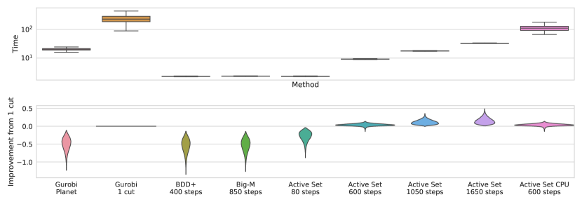
(a) Speed-accuracy trade-offs of Active Set for different iteration ranges and computing devices.

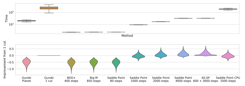
(b) Speed-accuracy trade-offs of Saddle Point for different iteration ranges and computing devices.

Figure 1: Robustness margin for the SGD-trained network from Bunel et al. (2020a). Box plots: distribution of runtime in seconds. Violin plots: difference with the bounds obtained by Gurobi with a cut from $\mathcal{A}_{k}$ per neuron; higher is better, the width at a given value represents the proportion of problems for which this is the result. On average, both Active Set and Saddle Point achieve bounds tighter than Gurobi 1 cut with a smaller runtime.

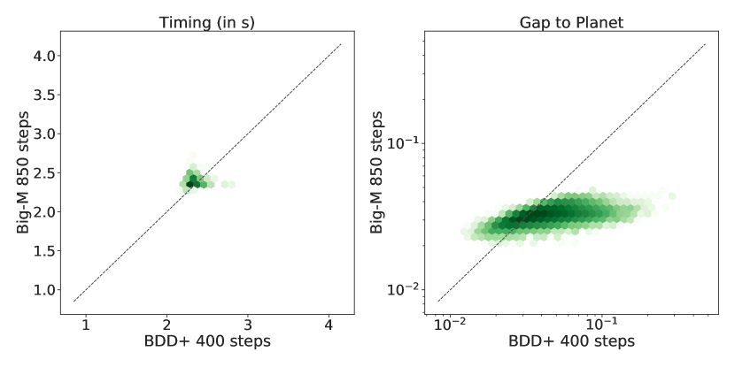
(a) Comparison of runtime (left) and gap to Gurobi Planet bounds (right). For the latter, lower is better.

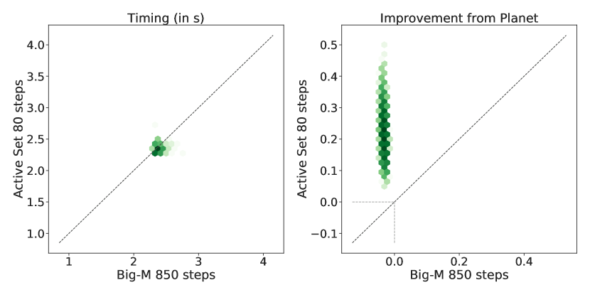
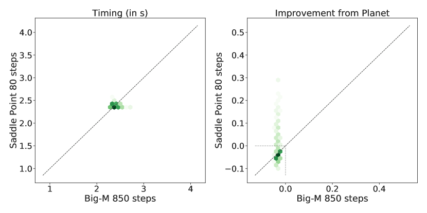
(b) Comparison of runtime (Timing) and difference with the Gurobi Planet bounds (Improvement from Planet). For the latter, higher is better.

Figure 2: Pointwise comparison for a subset of the methods on the data presented in figure 1. Darker colour shades mean higher point density (on a logarithmic scale). The oblique dotted line corresponds to the equality.

Figure 1 shows the distribution of runtime and the bound improvement with respect to Gurobi cut for the SGD-trained network. For Gurobi cut, we only add the single most violated cut from $\mathcal{A}_{k}$ per neuron, due to the cost of repeatedly solving the LP. We tuned BDD+ and Big-M, the dual methods operating on the weaker relaxation (2), to have the same average runtime. They obtain bounds comparable to Gurobi Planet in one order less time. Initialised from $500$ Big-M iterations, at $600$ iterations, Active Set already achieves better bounds on average than Gurobi cut in around $1/20^{{th}}$ of the time. With a computational budget twice as large ($1050$ iterations) or four times as large ($1650$ iterations), the bounds significantly improve over Gurobi cut in a fraction of the time. Similar observations hold for Saddle Point which, especially when using fewer iterations, also exhibits a larger variance in terms of bounds tightness. In appendix H, we empirically demonstrate that the tightness of the Active Set bounds is strongly linked to our active set strategy (see $\S$4.2). Remarkably, even if our solvers are specifically designed to take advantage of GPU acceleration, executing them on CPU proves to be strongly competitive with Gurobi cut. Active Set produces better bounds in less time for the benchmark of Figure 1, while Saddle Point yields comparable speed-accuracy trade-offs.

8.2.1 Small computational budget

Figure 2 shows pointwise comparisons for the less expensive methods from figure 1, on the same data. Figure 2(a) shows the gap to the (Gurobi) Planet bound for BDD+ and our Big-M solver. Surprisingly, our Big-M solver is competitive with BDD+, achieving on average better bounds than BDD+, in the same time. Figure 2(b) shows the improvement over Planet bounds for Big-M compared to those of few ($80$) Active Set and Saddle Point iterations. Active Set returns markedly better bounds than Big-M in the same time, demonstrating the benefit of operating (at least partly) on the tighter dual (6). On the other hand, Saddle Point is rarely beneficial with respect to Big-M when running it for a few iterations.

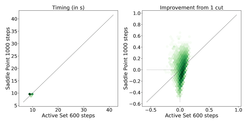
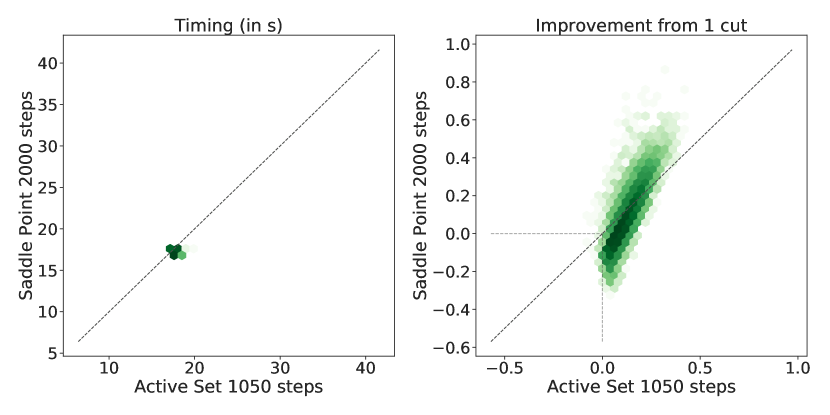
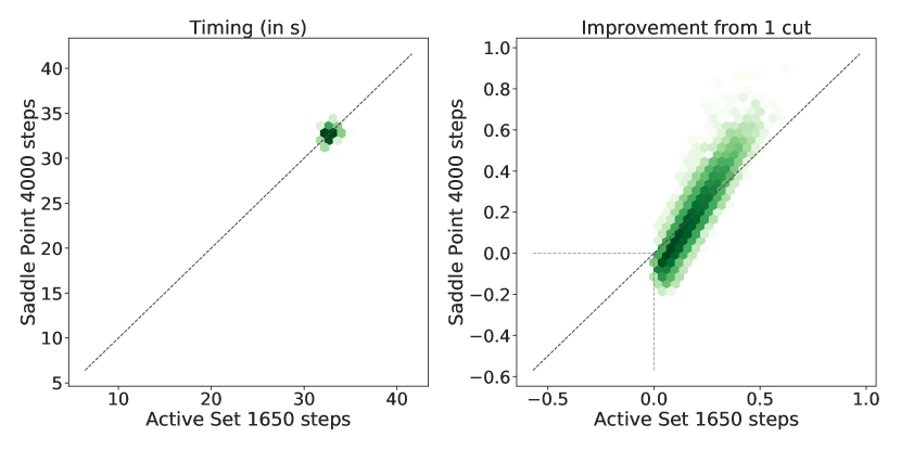
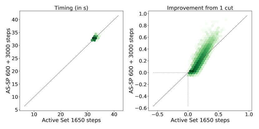
Figure 3: Pointwise comparison between our proposed solvers on the data presented in figure 1. Darker colour shades mean higher point density (on a logarithmic scale). The oblique dotted line corresponds to the equality.

8.2.2 Larger computational budget

Figure 3 compares the performance of Active Set and Saddle Point for different runtimes, once again on the data from figure 1. While Active Set yields better average bounds when fewer iterations are employed, the performance gap shrinks with increasing computational budgets, and AS-SP (Active Set initialization to Saddle Point) yields tighter average bounds than Active Set in the same time. Differently from Active Set, the memory footprint of Saddle Point does not increase with the number of iterations (see $\S$5). Therefore, we believe the Frank-Wolfe-based algorithm is particularly convenient in incomplete verification settings that require tight bounds.

8.3 Complete Verification

We next evaluate the performance on complete verification, verifying the adversarial robustness of a network to perturbations in $\ell_{\infty}$ norm on a subset of the dataset by Lu and Kumar (2020). We replicate the experimental setting from Bunel et al. (2020a).

Network Name	No. of Properties	Network Architecture
BASE Model	100	Conv2d(3,8,4, stride=2, padding=1) Conv2d(8,16,4, stride=2, padding=1) linear layer of 100 hidden units linear layer of 10 hidden units (Total ReLU activation units: 3172)
WIDE	100	Conv2d(3,16,4, stride=2, padding=1) Conv2d(16,32,4, stride=2, padding=1) linear layer of 100 hidden units linear layer of 10 hidden units (Total ReLU activation units: 6244)
DEEP	100	Conv2d(3,8,4, stride=2, padding=1) Conv2d(8,8,3, stride=1, padding=1) Conv2d(8,8,3, stride=1, padding=1) Conv2d(8,8,4, stride=2, padding=1) linear layer of 100 hidden units linear layer of 10 hidden units (Total ReLU activation units: 6756)

Table 1: For each complete verification experiment, the network architecture used and the number of verification properties tested, a subset of the dataset by Lu and Kumar (2020). Each layer but the last is followed by a ReLU activation function.

Lu and Kumar (2020) provide, for a subset of the CIFAR-10 test set, a verification radius $\epsilon_{ver}$ defining the small region over which to look for adversarial examples (input points for which the output of the network is not the correct class) and a (randomly sampled) non-correct class to verify against. The verification problem is formulated as the search for an adversarial example, carried out by minimizing the difference between the ground truth logit and the target logit. If the minimum is positive, we have not succeeded in finding a counter-example, and the network is robust. The $\epsilon_{ver}$ radius was tuned to meet a certain “problem difficulty” via binary search, employing a Gurobi-based bounding algorithm (Lu and Kumar, 2020). This characteristic makes the dataset an appropriate testing ground for tighter relaxations like the one by Anderson et al. (2020) ($\S$2.2). The networks are robust on all the properties we employed. Three different network architectures of different sizes are used. A “Base” network with $3172$ ReLU activations, and two networks with roughly twice as many activations: one “Deep”, the other “Wide”. Details can be found in Table 1. We restricted the original dataset to $100$ properties per network so as to mirror the setup of the recent VNN-COMP competition (VNN-COMP, 2020).

We compare the effect on final verification time of using the different bounding methods in $\S$8.2 within BaBSR, a branch and bound algorithm presented by Bunel et al. (2020b). In BaBSR, branching is carried out by splitting an unfixed ReLU into its passing and blocking phases (see $\S$6.2 for a description of branch and bound). In order to determine which ReLU to split on, BaBSR employs an inexpensive heuristic based on the bounding algorithm by Wong and Kolter (2018). The goal of the heuristic is to assess which ReLU induces maximum change in the domain’s lower bound when made unambiguous. When stratifying two bounding algorithms (see $\S$6.2) we denote the resulting method by the names of both the looser and the tighter bounding method, separated by a plus sign (for instance, Big-M + Active Set). In addition to assessing the various bounding methods within BaBSR, we compare against the following complete verification algorithms:

• MIP $\mathcal{A}_{k}$ encodes problem (1) as a Big-M MIP (Tjeng et al., 2019) and solves it in Gurobi by adding cutting planes from $\mathcal{A}_{k}$. This mirrors the original experiments from Anderson et al. (2020).

• ERAN (Singh et al., 2020), a state-of-the-art complete verification toolbox. Results on the dataset by Lu and Kumar (2020) are taken from the recent VNN-COMP competition (VNN-COMP, 2020).

Base Wide Deep Method time(s) sub-problems $\%$Timeout time(s) sub-problems $\%$Timeout time(s) sub-problems $\%$Timeout BDD+ BaBSR $883.55$ $82\,699.40$ $22.00$ $568.25$ $43\,751.88$ $13.00$ $281.47$ $10\,763.48$ $5.00$ Big-M BaBSR $826.60$ $68\,582.00$ $19.00$ $533.79$ $35\,877.24$ $12.00$ $253.37$ $9346.78$ $4.00$ A. Set 100 it. BaBSR $422.32$ $9471.90$ $7.00$ $169.73$ $1873.36$ $3.00$ $227.26$ $2302.16$ $2.00$ Big-M + A. Set 100 it. BaBSR $415.20$ $10\,449.10$ $7.00$ $163.02$ $2402.28$ $3.00$ $199.70$ $2709.60$ $2.00$ G. Planet + G. 1 cut BaBSR $949.06$ $1572.10$ $15.00$ $762.42$ $514.02$ $6.00$ $799.71$ $391.70$ $2.00$ MIP $\mathcal{A}_{k}$ $3227.50$ $226.24$ $82.00$ $2500.70$ $100.93$ $64.00$ $3339.37$ $434.57$ $91.00$ ERAN $805.89$ - $5.00$ $632.12$ - $9.00$ $545.72$ - $0.00$

Table 2: We compare average solving time, average number of solved sub-problems and the percentage of timed out properties on data from Lu and Kumar (2020). The best dual iterative method is highlighted in bold.

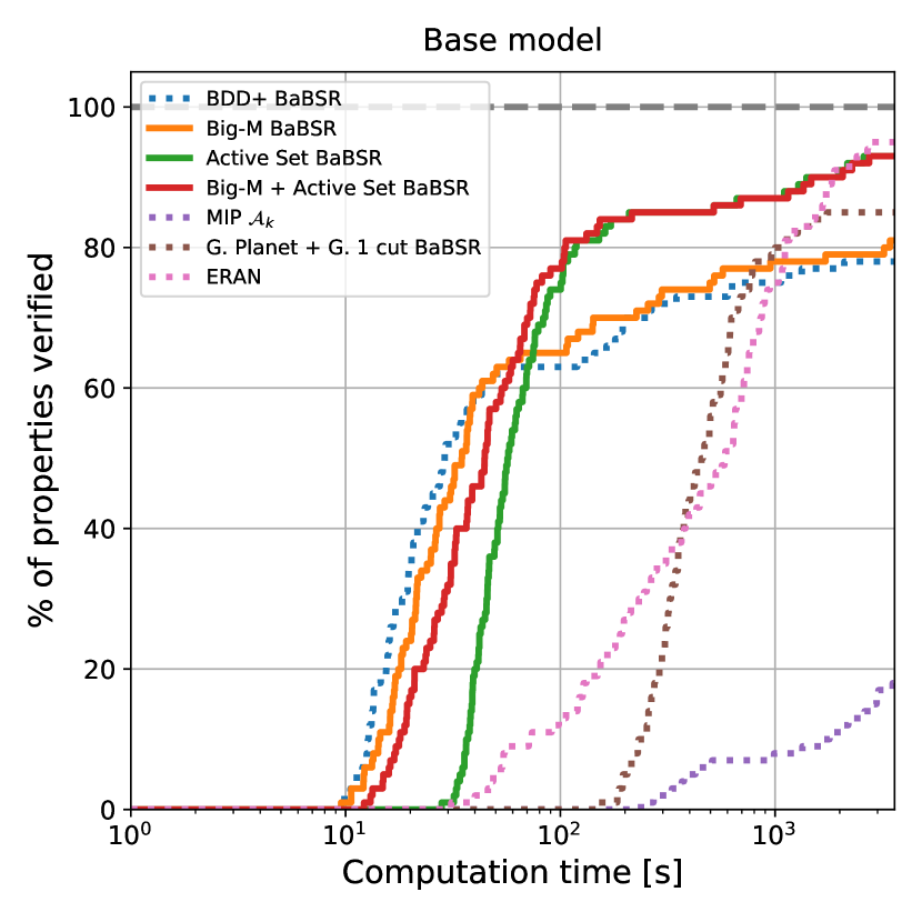
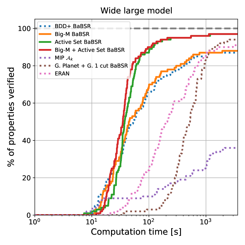
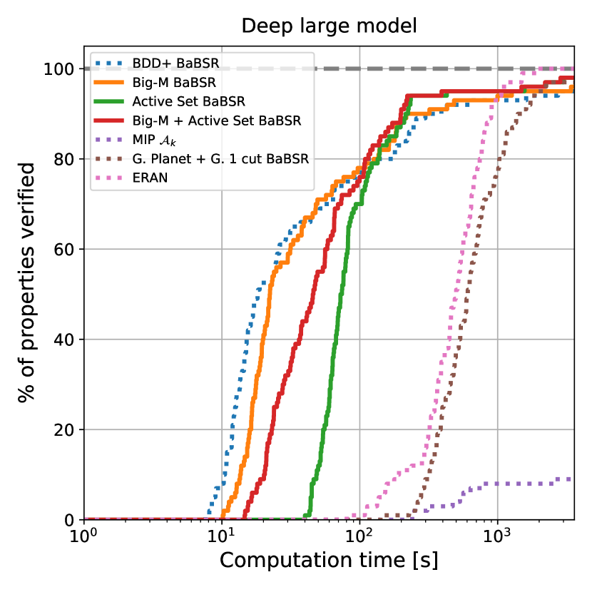
Figure 4: Cactus plots on properties from Lu and Kumar (2020), displaying the percentage of solved properties as a function of runtime. Baselines are represented by dotted lines.

We use $100$ iterations for BDD+ (as done by Bunel et al. (2020a)) and $180$ for Big-M, which was tuned to employ roughly the same time per bounding computation as BDD+. We re-employed the same hyper-parameters for Big-M, Active Set and Saddle Point, except the number of iterations. For dual iterative algorithms, we solve 300 subproblems at once for the base network and 200 for the deep and wide networks (see $\S$6.1). Additionally, dual variables are initialised from their parent node’s bounding computation. As in Bunel et al. (2020a), the time-limit is kept at one hour.

8.3.1 Inexpensively overcoming the convex barrier

Figure 2(b) in the previous section shows that Active Set can yield a relatively large improvement over Gurobi Planet bounds, the convex barrier as defined by Salman et al. (2019), in a few iterations. In light of this, we start our experimental evaluation by comparing the performance of $100$ iterations of Active Set (within BaBSR) with the relevant baselines.

Figure 4 and Table 2 show that Big-M performs competitively with BDD+. With respect to the methods operating on the looser formulation (2), Active Set verifies a larger share of properties and yields faster average verification. This demonstrates the benefit of tighter bounds ($\S$8.2) in complete verification. On the other hand, the poor performance of MIP + $\mathcal{A}_{k}$ and of Gurobi Planet + Gurobi 1 cut, tied to scaling limitations of off-the-shelf solvers, shows that tighter bounds are effective only if they can be computed efficiently. Nevertheless, the difference in performance between the two Gurobi-based methods confirms that customised Branch and Bound solvers (BaBSR) are preferable to generic MIP solvers, as observed by Bunel et al. (2020b) on the looser Planet relaxation. Moreover, the stratified bounding system allows us to retain some of the speed of Big-M on easier properties, without sacrificing Active Set’s gains on the harder ones. Finally, while ERAN verifies $2\%$ more properties than Active Set on two networks, BaBSR (with any dual bounding algorithm) is faster on most of the properties. BaBSR-based results could be further improved by employing the learned branching strategy presented by Lu and Kumar (2020): in this work, we focused on the bounding component of branch and bound.

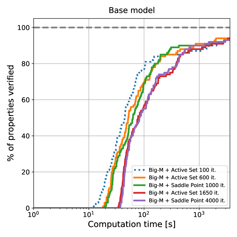
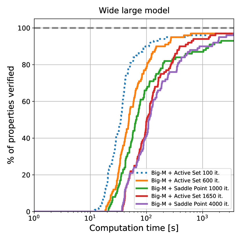
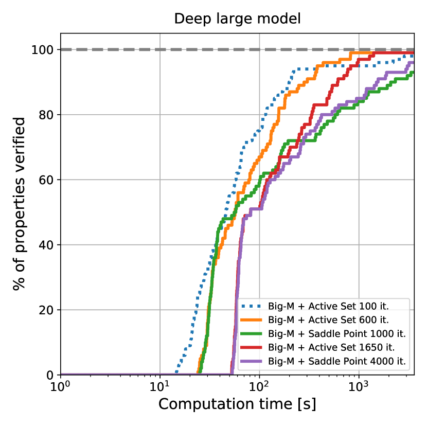
Figure 5: Cactus plots on properties from Lu and Kumar (2020), displaying the percentage of solved properties as a function of runtime. Comparison of best performing method from figure 4 with tighter bounding schemes.

Base Wide Deep Method time(s) sub-problems $\%$Timeout time(s) sub-problems $\%$Timeout time(s) sub-problems $\%$Timeout Big-M + Active Set 100 it. $415.20$ $10\,449.10$ $7.00$ $163.02$ $2402.28$ $3.00$ $199.70$ $2709.60$ $2.00$ Big-M + Active Set 600 it. $360.16$ $4806.14$ $6.00$ $181.27$ $1403.90$ $3.00$ $148.06$ $1061.90$ $1.00$ Big-M + Saddle Point 1000 it. $382.15$ $5673.04$ $7.00$ $417.41$ $1900.90$ $7.00$ $540.68$ $2551.62$ $7.00$ Big-M + Active Set 1650 it. $463.00$ $7484.54$ $6.00$ $285.99$ $1634.98$ $3.00$ $250.52$ $1119.00$ $1.00$ Big-M + Saddle Point 4000 it. $434.92$ $4859.68$ $7.00$ $402.86$ $1703.48$ $3.00$ $482.93$ $1444.20$ $4.00$

Table 3: We compare average solving time, average number of solved sub-problems and the percentage of timed out properties on data from Lu and Kumar (2020). The best result is highlighted in bold. Comparison of best performing method from figure 4 with tighter bounding schemes within BaBSR.

8.3.2 Varying speed-accuracy trade-offs

The results in $\S$8.3.1 demonstrate that a small yet inexpensive tightening of the Planet bounds yields large complete verification improvements. We now investigate the effect of employing even tighter, yet more costly, bounds from our solvers. To this end, we compare $100$ iterations of Active Set with more expensive bounding schemes from our incomplete verification experiments ($\S$8.2). All methods were stratified along Big-M to improve performance on easier properties (see $\S$6.2) and employed within BaBSR. Figure 5 and Table 3 show results for two different bounding budgets: $600$ iterations of Active Set or $1000$ of Saddle Point, $1650$ iterations of Active Set or $4000$ of Saddle Point (see figure 3). Despite their ability to prune more subproblems, due to their large computational cost, tighter bounds do not necessarily correspond to shorter overall verification times. Running Active Set for $600$ iterations of Active Set leads to faster verification of the harder properties while slowing it down for the easier ones. On the base and deep model, the benefits lead to a smaller average runtime (Table 3). This does not happen on the wide network, for which not enough subproblems are pruned. On the other hand, $1650$ Active Set iterations do not prune enough subproblems for their computational overhead, leading to slower formal verification. The behavior of Saddle Point mirrors what seen for incomplete verification: while it does not perform as well as Active Set for small computational budgets, the gap shrinks when the algorithms are run for more iterations and it is very competitive with Active Set on the base network. Keeping in mind that the memory cost of each variable addition to the active set is larger in complete verification due to subproblem batching (see 6.1), Saddle Point constitutes a valid complete verification alternative in settings where memory is critical.

9 Discussion

The vast majority of neural network bounding algorithms focuses on (solving or loosening) a popular triangle-shaped relaxation, referred to as the “convex barrier” for verification. Relaxations that are tighter than this convex barrier have been recently introduced, but the complexity of the standard solvers for such relaxations hinders their applicability. We have presented two different sparse dual solvers for one such relaxation, and empirically demonstrated that they can yield significant formal verification speed-ups. Our results show that tightness, when paired with scalability, is key to the efficiency of neural network verification and instrumental in the definition of a more appropriate “convex barrier”. We believe that new customised solvers for similarly tight relaxations are a crucial avenue for future research in the area, possibly beyond piecewise-linear networks. Finally, as it is inevitable that tighter bounds will come at a larger computational cost, future verification systems will be required to recognise a priori whether tight bounds are needed for a given property. A possible solution to this problem could rely on learning algorithms.

A Limitations of Previous Dual Approaches

In this section, we show that previous dual derivations (Bunel et al., 2020a; Dvijotham et al., 2018) violate Fact 1. Therefore, they are not efficiently applicable to problem (3), motivating our own derivation in section 3.

We start from the approach by Dvijotham et al. (2018), which relies on relaxing equality constraints (1b), (1c) from the original non-convex problem (1). Dvijotham et al. (2018) prove that this relaxation corresponds to solving convex problem (2), which is equivalent to the Planet relaxation (Ehlers, 2017), to which the original proof refers. As we would like to solve tighter problem (3), the derivation is not directly applicable. Relying on intuition from convex analysis applied to duality gaps (Lemaréchal, 2001), we conjecture that relaxing the composition (1c) $\circ$ (1b) might tighten the primal problem equivalent to the relaxation, obtaining the following dual:

$$\begin{split}\max_{\bm{\mu}}\min_{\mathbf{x}}&\quad W_{n}\mathbf{x}_{n-1}+\mathbf{b}_{n}+\sum_{k=1}^{n-1}\bm{\mu}_{k}^{T}\left(\mathbf{x}_{k}-\max\left\{W_{k}\mathbf{x}_{k-1}+\mathbf{b}_{k},0\right\}\right)\\ \text{s.t. }\quad&\mathbf{l}_{k}\leq\mathbf{x}_{k}\leq\mathbf{u}_{k}\qquad\qquad k\in\left\llbracket 1,n-1\right\rrbracket,\\ &\mathbf{x}_{0}\in\mathcal{C}.\end{split}$$ (16)

Unfortunately dual (16) requires an LP (the inner minimisation over $\mathbf{x}$, which in this case does not decompose over layers) to be solved exactly to obtain a supergradient and any time a valid bound is needed. This is markedly different from the original dual by  Dvijotham et al. (2018), which had an efficient closed-form for the inner problems.

The derivation by Bunel et al. (2020a), instead, operates by substituting (1c) with its convex hull and solving its Lagrangian Decomposition dual. The Decomposition dual for the convex hull of (1c) $\circ$ (1b) (i.e., $\mathcal{A}_{k}$) takes the following form:

$$\begin{split}\max_{\bm{\rho}}\min_{\mathbf{x},\mathbf{z}}\ &W_{n}\mathbf{x}_{A,n-1}+\mathbf{b}_{n}+\sum_{k=1}^{n-1}\bm{\rho}_{k}^{T}\left(\mathbf{x}_{B,k}-\mathbf{x}_{A,k}\right)\\[5.0pt] \text{s.t. }\quad&\mathbf{x}_{0}\in\mathcal{C},\\ &(\mathbf{x}_{B,k},W_{n}\mathbf{x}_{A,n-1}+\mathbf{b}_{n},\mathbf{z}_{k})\in\mathcal{A}_{\text{dec},k}\qquad k\in\left\llbracket 1,n-1\right\rrbracket,\end{split}$$ (17)

where $\mathcal{A}_{\text{dec},k}$ corresponds to $\mathcal{A}_{k}$ with the following substitutions: $\mathbf{x}_{k}\rightarrow\mathbf{x}_{B,k}$, and $\mathbf{\hat{x}}_{k}\rightarrow W_{n}\mathbf{x}_{A,n-1}+\mathbf{b}_{n}$. It can be easily seen that the inner problems (the inner minimisation over $\mathbf{x}_{A,k},\mathbf{x}_{B,k}$, for each layer $k>0$) are an exponentially sized LP. Again, this differs from the original dual on the Planet relaxation (Bunel et al., 2020a), which had an efficient closed-form for the inner problems.

B Dual Initialisation

Algorithm 3 Big-M solver

1:function bigm_compute_bounds($\{W_{k},\mathbf{b}_{k},\mathbf{l}_{k},\mathbf{u}_{k},\hat{\mathbf{l}}_{k},\hat{\mathbf{u}}_{k}\}_{k=1..n}$)

2:   Initialise duals $\bm{\alpha}^{0},\bm{\beta}^{0}_{\mathcal{M}}$ using interval propagation bounds (Gowal et al., 2018)

3:   for $t\in\llbracket 1,T-1\rrbracket$ do

4:      $\mathbf{x}^{*,t},\mathbf{z}^{*,t}\in$ $\operatorname*{\arg\!\min}_{\mathbf{x},\mathbf{z}}\mathcal{L}_{\mathcal{M}}(\mathbf{x},\mathbf{z},\bm{\alpha}^{t},\bm{\beta}^{t}_{\mathcal{M}})$ using (20)-(21)

5:      $\bm{\alpha}^{t+1},\bm{\beta}^{t+1}_{\mathcal{M}}\leftarrow[\bm{\alpha}^{t},\bm{\beta}^{t}]+H[\nabla_{\bm{\alpha}}d_{\mathcal{M}}(\bm{\alpha},\bm{\beta}),\nabla_{\bm{\beta}_{\mathcal{M}}}d_{\mathcal{M}}(\bm{\alpha},\bm{\beta})]$ $\triangleright$ supergradient step, using (22)

6:      $\bm{\alpha}^{t+1},\bm{\beta}^{t+1}_{\mathcal{M}}\leftarrow\max(\bm{\alpha}^{t+1},0),\max(\bm{\beta}^{t+1}_{\mathcal{M}},0)\qquad$ $\triangleright$ dual projection

7:   end for

8:   return $\min_{\mathbf{x},\mathbf{z}}\mathcal{L}_{\mathcal{M}}(\mathbf{x},\mathbf{z},\bm{\alpha}^{T},\bm{\beta}^{T}_{\mathcal{M}})$

9:end function

As shown in section 3, the Active Set solver reduces to a dual solver for the Big-M relaxation (2) if the active set $\mathcal{B}$ is kept empty throughout execution. We employ this Big-M solver as dual initialization for both Active Set ($\S$4) and Saddle Point ($\S$5). We demonstrate experimentally in $\S$8 that, when used as a stand-alone solver, our Big-M solver is competitive with previous dual algorithms for problem (2).

The goal of this section is to explicitly describe the Big-M solver, which is summarised in algorithm 3. We point out that, in the notation of restricted variable sets from section 4, $\bm{\beta}_{\mathcal{M}}:=\bm{\beta}_{\emptyset}$. We now describe the equivalence between the Big-M and Planet relaxations, before presenting the solver in section B.3 and the dual it operates on in section B.2.

B.1 Equivalence to Planet

As previously shown (Bunel et al., 2018), the Big-M relaxation ($\mathcal{M}_{k}$, when considering the $k$-th layer only) in problem (2) is equivalent to the Planet relaxation by Ehlers (2017). Then, due to strong duality, our Big-M solver (section B.2) and the solvers by Bunel et al. (2020a); Dvijotham et al. (2018) will all converge to the bounds from the solution of problem (2). In fact, the Decomposition-based method (Bunel et al., 2020a) directly operates on the Planet relaxation, while Dvijotham et al. (2018) prove that their dual is equivalent to doing so.

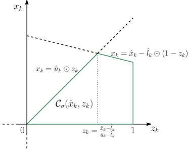
Figure 6: $\mathcal{M}_{k}$ plotted on the $(\mathbf{z}_{k},\mathbf{x}_{k})$ plane, under the assumption that $\hat{\mathbf{l}}_{k}\leq 0\text{ and }\hat{\mathbf{u}}_{k}\geq 0$.

On the $k$-th layer, the Planet relaxation takes the following form:

$$\begin{split}\mathcal{P}_{k}:=\begin{cases}\text{if }\hat{\mathbf{l}}_{k}\leq 0\text{ and }\hat{\mathbf{u}}_{k}\geq 0:&\\ &\mathbf{x}_{k}\geq 0,\quad\mathbf{x}_{k}\geq\mathbf{\hat{x}}_{k},\\ &\mathbf{x}_{k}\leq\mathbf{\hat{u}_{k}}\odot(\mathbf{\hat{x}}_{k}-\mathbf{\hat{l}}_{k})\odot\left(1/(\mathbf{\hat{u}_{k}}-\mathbf{\hat{l}_{k}})\right).\\ \text{if }\hat{\mathbf{u}}_{k}\leq 0:&\\ &\mathbf{x}_{k}=0.\\ \text{if }\hat{\mathbf{l}}_{k}\geq 0:&\\ &\mathbf{x}_{k}=\mathbf{\hat{x}}_{k}.\end{cases}\end{split}$$ (18)

It can be seen that $\mathcal{P}_{k}=\text{Proj}_{\mathbf{x},\mathbf{\hat{x}}}\left(\mathcal{M}_{k}\right)$, where $\text{Proj}_{\mathbf{x},\mathbf{\hat{x}}}$ denotes projection on the $\mathbf{x},\mathbf{\hat{x}}$ hyperplane. In fact, as $\mathbf{z}_{k}$ does not appear in the objective of the primal formulation (2), but only in the constraints, this means assigning it the value that allows the largest possible feasible region. This is trivial for passing or blocking ReLUs. For the ambiguous case, instead, Figure 6 (on a single ReLU) shows that $z_{k}=\frac{\hat{x}_{k}-\hat{l}_{k}}{\hat{u}_{k}-\hat{l}_{k}}$ is the correct assignment.

B.2 Big-M Dual

As evident from problem (3), $\mathcal{A}_{k}\subseteq\mathcal{M}_{k}$. If we relax all constraints in $\mathcal{M}_{k}$ (except, again, the box constraints), we are going to obtain a dual with a strict subset of the variables in problem (6). The Big-M dual is a specific instance of the Active Set dual (7) where $\mathcal{B}=\emptyset$, and it takes the following form:

$$\max_{(\bm{\alpha},\bm{\beta})\geq 0} d_{\mathcal{M}}(\bm{\alpha},\bm{\beta}_{\mathcal{M}})\qquad\text{where:}\qquad d_{\mathcal{M}}(\bm{\alpha},\bm{\beta}_{\mathcal{M}}):=\min_{\mathbf{x},\mathbf{z}}\enskip\mathcal{L}_{\mathcal{M}}(\mathbf{x},\mathbf{z},\bm{\alpha},\bm{\beta}_{\mathcal{M}}),$$ (19)

$$\mathcal{L}_{\mathcal{M}}(\mathbf{x},\mathbf{z},\bm{\alpha},\bm{\beta}_{\mathcal{M}})= \left[\begin{array}[]{l}-\sum_{k=0}^{n-1}\left(\bm{\alpha}_{k}-W_{k+1}^{T}\bm{\alpha}_{k+1}-(\bm{\beta}_{k,0}+\bm{\beta}_{k,1}-W_{k+1}^{T}\bm{\beta}_{k+1,1})\right)^{T}\mathbf{x}_{k}\\ +\sum_{k=1}^{n-1}\mathbf{b}_{k}^{T}\bm{\alpha}_{k}-\sum_{k=1}^{n-1}\left(\bm{\beta}_{k,0}\odot\hat{\mathbf{u}}_{k}+\bm{\beta}_{k,1}\odot\hat{\mathbf{l}}_{k}\right)^{T}\mathbf{z}_{k}\\ +\sum_{k=1}^{n-1}(\hat{\mathbf{l}}_{k}-\mathbf{b}_{k})^{T}\bm{\beta}_{k,1}\end{array}\right.$$

s.t. $$\mathbf{x}_{0}\in\mathcal{C},\qquad(\mathbf{x}_{k},\mathbf{z}_{k})\in[\mathbf{l}_{k},\mathbf{u}_{k}]\times[\mathbf{0},\ \mathbf{1}]\qquad k\in\llbracket 1,n-1\rrbracket.$$

B.3 Big-M solver

We initialise dual variables from interval propagation bounds (Gowal et al., 2018): this can be easily done by setting all dual variables except $\bm{\alpha}_{n}$ to $0$. Then, we can maximize $d_{\mathcal{M}}(\bm{\alpha},\bm{\beta})$ via projected supergradient ascent, exactly as described in section 4 on a generic active set $\mathcal{B}$. All the computations in the solver follow from keeping $\mathcal{B}=\emptyset$ in $\S$4. We explicitly report them here for the reader’s convenience.

Let us define the following shorthand for the primal coefficients:

$$\begin{gathered}\bm{f}_{\mathcal{M},k}(\bm{\alpha},\bm{\beta}_{\mathcal{M}})=\left(\bm{\alpha}_{k}-W_{k+1}^{T}\bm{\alpha}_{k+1}-(\bm{\beta}_{k,0}+\bm{\beta}_{k,1}-W_{k+1}^{T}\bm{\beta}_{k,1})\right)\\ \bm{g}_{\mathcal{M},k}(\bm{\beta}_{\mathcal{M}})=\bm{\beta}_{k,0}\odot\hat{\mathbf{u}}_{k}+\bm{\beta}_{k,1}\odot\hat{\mathbf{l}}_{k}.\end{gathered}$$

The minimisation of the Lagrangian $\mathcal{L}_{\mathcal{M}}(\mathbf{x},\mathbf{z},\bm{\alpha},\bm{\beta})$ over the primals for $k\in\llbracket 1,n-1\rrbracket$ is as follows:

$$\begin{gathered}\mathbf{x}_{k}^{*}=\mathds{1}_{\bm{f}_{\mathcal{M},k}(\bm{\alpha},\bm{\beta}_{\mathcal{M}})\geq 0}\odot\hat{\mathbf{u}}_{k}+\mathds{1}_{\bm{f}_{\mathcal{M},k}(\bm{\alpha},\bm{\beta}_{\mathcal{M}})<0}\odot\hat{\mathbf{l}}_{k}\qquad\mathbf{z}_{k}^{*}=\mathds{1}_{\bm{g}_{\mathcal{M},k}(\bm{\beta}_{\mathcal{M}})\geq 0}\odot\mathbf{1}\\[8.0pt] \end{gathered}$$ (20)

For $k=0$, instead (assuming, as $\S$4 that this can be done efficiently):

$$\mathbf{x}^{*}_{0}\in\operatorname*{\arg\!\min}_{\mathbf{x}_{0}}\quad\bm{f}_{\mathcal{M},k}(\bm{\alpha},\bm{\beta}_{\mathcal{M}})^{T}\mathbf{x}_{0}\qquad\quad\text{s.t. }\quad\mathbf{x}_{0}\in\mathcal{C}.$$ (21)

The supergradient over the Big-M dual variables $\bm{\alpha},\bm{\beta}_{k,0},\bm{\beta}_{k,1}$ is computed exactly as in $\S$4 and is again a subset of the supergradient of the full dual problem (6). We report it for completeness. For each $k\in\llbracket 0,n-1\rrbracket$:

$$\begin{gathered}\nabla_{\bm{\alpha}_{k}}d(\bm{\alpha},\bm{\beta})=W_{k}\mathbf{x}^{*}_{k-1}+\mathbf{b}_{k}-\mathbf{x}^{*}_{k},\quad\nabla_{\bm{\beta}_{k,0}}d(\bm{\alpha},\bm{\beta})=\mathbf{x}_{k}-\mathbf{z}_{k}\odot\hat{\mathbf{u}}_{k},\\ \nabla_{\bm{\beta}_{k,1}}d(\bm{\alpha},\bm{\beta})=\mathbf{x}_{k}-\left(W_{k}\mathbf{x}_{k-1}+\mathbf{b}_{k}\right)+\left(1-\mathbf{z}_{k}\right)\odot\hat{\mathbf{l}}_{k}.\end{gathered}$$ (22)

C Implementation Details for Saddle Point

In this section, we present details of the Saddle Point solver that were omitted from the main paper. We start with the choice of price caps $\bm{\mu}_{k}$ on the Lagrangian multipliers ($\S$C.1), and conclude with a description of our primal initialisation procedure ($\S$C.2).

C.1 Constraint Price Caps

Price caps $\bm{\mu}$ containing the optimal dual solution to problem (6) can be found via binary search (see $\S$5.1). However, such a strategy might require running Saddle Point to convergence on several instances of problem (13). Therefore, in practice, we employ a heuristic to set constraint caps to a reasonable approximation.

Given duals $(\bm{\alpha}^{0},\bm{\beta}^{0})$ from the dual initialization procedure (algorithm 1 or algorithm 3, depending on the computational budget), for each $k\in\left\llbracket 1,n-1\right\rrbracket$ we set $\bm{\mu}_{k}$ as follows:

$$\bm{\mu}_{\alpha,k} =\begin{cases}\bm{\alpha}_{k}^{0}&\text{if }\bm{\alpha}_{k}^{0}>0\\ c_{\alpha,k}&\text{otherwise}\end{cases}$$ (23)

$$\bm{\mu}_{\beta,k} =\begin{cases}\begin{array}[]{l}\sum_{I_{k}\in 2^{W_{k}}}\bm{\beta}_{k}^{0}\end{array}&\text{if }\begin{array}[]{l}\sum_{I_{k}\in 2^{W_{k}}}\bm{\beta}_{k}^{0}\end{array}>0\\[5.0pt] c_{\beta,k}&\text{otherwise},\end{cases}$$

where $c_{\alpha,k}$ and $c_{\beta,k}$ are small positive constants. In other words, we cap the (sums over) dual variables to their values at initialization if these are non-zero, and we allow dual variables to turn positive otherwise. While a larger feasible region (for instance, setting $\bm{\mu}_{\alpha,k}=\max_{i}\bm{\alpha}_{k}[i]\odot\mathbf{1}$, $\bm{\mu}_{\beta,k}=\max_{i}\sum_{I_{k}\in 2^{W_{k}}}\bm{\beta}_{k}^{0}[i]\odot\mathbf{1}$) might yield tighter bounds at convergence, we found assignment (23) to be more effective on the iteration budgets employed in $\S$8.2,$\S$8.3.

C.2 Primal Initialization

If we invert the minimization and maximization, our saddle-point problem (13) can be seen as a non-smooth minimization problem (the minimax theorem holds):

$$\min_{\mathbf{x},\mathbf{z}}\max_{\bm{\alpha},\bm{\beta}} \left[\begin{array}[]{l}\sum_{k=1}^{n-1}\bm{\alpha}_{k}^{T}\left(W_{k}\mathbf{x}_{k-1}+\mathbf{b}_{k}-\mathbf{x}_{k}\right)+\sum_{k=1}^{n-1}\bm{\beta}_{k,0}^{T}\left(\mathbf{x}_{k}-\mathbf{z}_{k}\odot\hat{\mathbf{u}}_{k}\right)\\ +\sum_{k=1}^{n-1}\sum_{I_{k}\in\mathcal{E}_{k}}\bm{\beta}_{k,I_{k}}^{T}\left(\begin{array}[]{l}\left(W_{k}\odot I_{k}\odot\check{L}_{k-1}\right)\diamond(1-\mathbf{z}_{k})\\ -\mathbf{b}_{k}\odot\mathbf{z}_{k}-\left(W_{k}\odot\left(1-I_{k}\right)\odot\check{U}_{k-1}\right)\diamond\mathbf{z}_{k}\\ -\left(W_{k}\odot I_{k}\right)\mathbf{x}_{k-1}+\mathbf{x}_{k}\end{array}\right)\\ +\sum_{k=1}^{n-1}\bm{\beta}_{k,1}^{T}\left(\mathbf{x}_{k}-\left(W_{k}\mathbf{x}_{k-1}+\mathbf{b}_{k}\right)+\left(1-\mathbf{z}_{k}\right)\odot\hat{\mathbf{l}}_{k}\right)+W_{n}\mathbf{x}_{n-1}+\mathbf{b}_{n}\end{array}\right.\qquad$$ (24)

s.t. $$\mathbf{x}_{0}\in\mathcal{C},$$

$$(\mathbf{x}_{k},\mathbf{z}_{k})\in[\mathbf{l}_{k},\mathbf{u}_{k}]\times[\mathbf{0},\ \mathbf{1}] k\in\left\llbracket 1,n-1\right\rrbracket,$$

$$\begin{array}[]{l}\bm{\alpha}_{k}\in[\mathbf{0},\bm{\mu}_{k,\alpha}]\\ \left(\bm{\beta}_{k}\geq\mathbf{0},\ \sum_{I_{k}\in\mathcal{E}_{k}\cup\{0,1\}}\bm{\beta}_{k,I_{k}}\leq\bm{\mu}_{k,\beta}\right)\end{array}\quad k\in\left\llbracket 1,n-1\right\rrbracket.$$

The “primal view” of problem (24) admits an efficient subgradient method, which we employ as primal initialization for the Saddle Point solver.

Technical details

The inner maximizers $(\bm{\alpha}^{*},\bm{\beta}^{*})$, which are required to obtain a valid subgradient, will be given in closed-form by the dual conditional gradients from equations (14), (15) (the objective is bilinear). Then, using the dual functions defined in (5), the subgradient over the linearly-many primal variables can be computed as $\bm{f}_{k}(\bm{\alpha}^{*},\bm{\beta}^{*})$ for $\mathbf{x}_{k}$ and $\bm{g}_{k}(\bm{\beta}^{*})$ for $\mathbf{z}_{k}$. After each subgradient step, the primals are projected to the feasible space: this is trivial for $\mathbf{x}_{k}$ and $\mathbf{z}_{k}$, which are box constrained, and can be efficiently performed for $\mathcal{C}$ in the common cases of $\ell_{\infty}$ or $\ell_{2}$ balls.

Simplified initialization

Due to the additional cost associated to masked forward-backward passes (see appendix G), the primal initialization procedure can be simplified by restricting the dual variables to the ones associated to the Big-M relaxation (appendix B). This can be done by substituting $\mathcal{E}_{k}\leftarrow\emptyset$ and $\bm{\beta}_{k}\leftarrow\bm{\beta}_{\emptyset,k}$ (see notation in $\S$4.1) in problem (24). A subgradient method for the resulting problem can then be easily adapted from the description above.

D Dual Derivations

We now derive problem (6), the dual of the full relaxation by Anderson et al. (2020) described in equation (3). The Active Set (equation (7)) and Big-M duals (equation (19)) can be obtained by removing $\bm{\beta}_{k,I_{k}}\forall\ I_{k}\in\mathcal{E}_{k}\setminus\mathcal{B}_{k}$ and $\bm{\beta}_{k,I_{k}}\forall\ I_{k}\in\mathcal{E}_{k}$, respectively. We employ the following Lagrangian multipliers:

$$\begin{split}\mathbf{x}_{k}\geq\mathbf{\hat{x}}_{k}&\Rightarrow\bm{\alpha}_{k},\\ \mathbf{x}_{k}\leq\hat{\mathbf{u}}_{k}\odot\mathbf{z}_{k}&\Rightarrow\bm{\beta}_{k,0},\\ \mathbf{x}_{k}\leq\mathbf{\hat{x}}_{k}-\hat{\mathbf{l}}_{k}\odot(1-\mathbf{z}_{k})&\Rightarrow\bm{\beta}_{k,1},\\ \mathbf{x}_{k}\leq\left(\begin{array}[]{l}\left(W_{k}\odot I_{k}\right)\mathbf{x}_{k-1}+\mathbf{z}_{k}\odot\mathbf{b}_{k}\\ -\left(W_{k}\odot I_{k}\odot\check{L}_{k-1}\right)\diamond(1-\mathbf{z}_{k})\\ +\left(W_{k}\odot\left(1-I_{k}\right)\odot\check{U}_{k-1}\right)\diamond\mathbf{z}_{k}\end{array}\right)&\Rightarrow\bm{\beta}_{k,I_{k}},\end{split}$$

and obtain, as a Lagrangian (using $\mathbf{\hat{x}}_{k}=W_{k}\mathbf{x}_{k-1}+\mathbf{b}_{k}$):

$$\mathcal{L}(\mathbf{x},\mathbf{z},\bm{\alpha},\bm{\beta})=\left[\begin{array}[]{l}\sum_{k=1}^{n-1}\bm{\alpha}_{k}^{T}\left(W_{k}\mathbf{x}_{k-1}+\mathbf{b}_{k}-\mathbf{x}_{k}\right)+\sum_{k=1}^{n-1}\bm{\beta}_{k,0}^{T}\left(\mathbf{x}_{k}-\mathbf{z}_{k}\odot\hat{\mathbf{u}}_{k}\right)\\ +\sum_{k=1}^{n-1}\sum_{I_{k}\in\mathcal{E}_{k}}\bm{\beta}_{k,I_{k}}^{T}\left(\begin{array}[]{l}\left(W_{k}\odot I_{k}\odot\check{L}_{k-1}\right)\diamond(1-\mathbf{z}_{k})-\left(W_{k}\odot I_{k}\right)\mathbf{x}_{k-1}\\ -\mathbf{b}_{k}\odot\mathbf{z}_{k}-\left(W_{k}\odot\left(1-I_{k}\right)\odot\check{U}_{k-1}\right)\diamond\mathbf{z}_{k}+\mathbf{x}_{k}\end{array}\right)\\ +\sum_{k=1}^{n-1}\bm{\beta}_{k,1}^{T}\left(\mathbf{x}_{k}-\left(W_{k}\mathbf{x}_{k-1}+\mathbf{b}_{k}\right)+\left(1-\mathbf{z}_{k}\right)\odot\hat{\mathbf{l}}_{k}\right)+W_{n}\mathbf{x}_{n-1}+\mathbf{b}_{n}\end{array}\right.$$

Let us use $\sum_{I_{k}}$ as shorthand for $\sum_{I_{k}\in\mathcal{E}_{k}\cup\{0,1\}}$. If we collect the terms with respect to the primal variables and employ dummy variables $\bm{\alpha}_{0}=0$, $\bm{\beta}_{0}=0$, $\bm{\alpha}_{n}=I$, $\bm{\beta}_{n}=0$, we obtain:

$$\mathcal{L}(\mathbf{x},\mathbf{z},\bm{\alpha},\bm{\beta})=\left[\begin{array}[]{l}-\sum_{k=0}^{n-1}\left(\begin{array}[]{l}\bm{\alpha}_{k}-W_{k+1}^{T}\bm{\alpha}_{k+1}-\sum_{I_{k}}\bm{\beta}_{k,I_{k}}\\ +\smash{\sum_{I_{k+1}}(W_{k+1}\odot I_{k+1})^{T}\bm{\beta}_{k+1,I_{k+1}}}\end{array}\right)^{T}\mathbf{x}_{k}\\ -\sum_{k=1}^{n-1}\left(\begin{array}[]{l}\sum_{I_{k}\in\mathcal{E}_{k}}\bm{\beta}_{k,I_{k}}\odot\mathbf{b}_{k}+\bm{\beta}_{k,1}\odot\hat{\mathbf{l}}_{k}+\bm{\beta}_{k,0}\odot\hat{\mathbf{u}}_{k}\\ +\sum_{I_{k}\in\mathcal{E}_{k}}\left(W_{k}\odot I_{k}\odot\check{L}_{k-1}\right)\diamond\bm{\beta}_{k,I_{k}}\\ +\sum_{I_{k}\in\mathcal{E}_{k}}\left(W_{k}\odot(1-I_{k})\odot\check{U}_{k-1}\right)\diamond\bm{\beta}_{k,I_{k}}\end{array}\right)^{T}\mathbf{z}_{k}\\ +\sum_{k=1}^{n-1}\mathbf{b}_{k}^{T}\bm{\alpha}_{k}+\sum_{k=1}^{n-1}\left(\sum_{I_{k}\in\mathcal{E}_{k}}(W_{k}\odot I_{k}\odot\check{L}_{k-1})\oblong\bm{\beta}_{k,I_{k}}+\bm{\beta}_{k,1}^{T}(\hat{\mathbf{l}}_{k}-\mathbf{b}_{k})\right)\end{array}\right.$$

which corresponds to the form shown in problem (6).

E Intermediate Bounds

A crucial quantity in both ReLU relaxations ($\mathcal{M}_{k}$ and $\mathcal{A}_{k}$) are intermediate pre-activation bounds $\hat{\mathbf{l}}_{k},\hat{\mathbf{u}}_{k}$. In practice, they are computed by solving a relaxation $\mathcal{C}_{k}$ (which might be $\mathcal{M}_{k}$, $\mathcal{A}_{k}$, or something looser) of (1) over subsets of the network (Bunel et al., 2020a). For $\hat{\mathbf{l}}_{i}$, this means solving the following problem (separately, for each entry $\hat{\mathbf{l}}_{i}[j]$):

$$\min_{\mathbf{x},\mathbf{\hat{x}},\mathbf{z}} \mathbf{\hat{x}}_{i}[j]$$ (25)

s.t. $$\mathbf{x}_{0}\in\mathcal{C}\hfil\hfil$$

$$\mathbf{\hat{x}}_{k+1}=W_{k+1}\mathbf{x}_{k}+\mathbf{b}_{k+1}, k\in\left\llbracket 0,i-1\right\rrbracket,$$

$$(\mathbf{x}_{k},\mathbf{\hat{x}}_{k},\mathbf{z}_{k})\in\mathcal{C}_{k} k\in\left\llbracket 1,i-1\right\rrbracket.$$

As (25) needs to be solved twice for each neuron (lower and upper bounds, changing the sign of the last layer’s weights) rather than once as in (3), depending on the computational budget, $\mathcal{C}_{k}$ might be looser than the relaxation employed for the last layer bounds (in our case, $\mathcal{A}_{k}$). In all our experiments, we compute intermediate bounds as the tightest bounds between the method by Wong and Kolter (2018) and Interval Propagation (Gowal et al., 2018).

Once pre-activation bounds are available, post-activation bounds can be simply computed as $\mathbf{l}_{k}=\max(\hat{\mathbf{l}}_{k},0),\mathbf{u}_{k}=\max(\hat{\mathbf{u}}_{k},0)$.

F Pre-activation Bounds in $\mathcal{A}_{k}$

We now highlight the importance of an explicit treatment of pre-activation bounds in the context of the relaxation by Anderson et al. (2020). In $\S$F.1 we will show through an example that, without a separate pre-activation bounds treatment, $\mathcal{A}_{k}$ could be looser than the less computationally expensive $\mathcal{M}_{k}$ relaxation. We then ($\S$F.2) justify our specific pre-activation bounds treatment by extending the original proof by Anderson et al. (2020).

The original formulation by Anderson et al. (2020) is the following:

$$\left.\begin{array}[]{l}\mathbf{x}_{k}\geq W_{k}\mathbf{x}_{k-1}+\mathbf{b}_{k}\\ \mathbf{x}_{k}\leq\left(\begin{array}[]{l}\left(W_{k}\odot I_{k}\right)\mathbf{x}_{k-1}+\mathbf{z}_{k}\odot\mathbf{b}_{k}\\ -\left(W_{k}\odot I_{k}\odot\check{L}_{k-1}\right)\diamond(1-\mathbf{z}_{k})\\ +\left(W_{k}\odot\left(1-I_{k}\right)\odot\check{U}_{k-1}\right)\diamond\mathbf{z}_{k}\end{array}\right)\ \forall I_{k}\in 2^{W_{k}}\\ (\mathbf{x}_{k},\mathbf{\hat{x}}_{k},\mathbf{z}_{k})\in[\mathbf{l}_{k},\mathbf{u}_{k}]\times[\hat{\mathbf{l}}_{k},\hat{\mathbf{u}}_{k}]\times[\mathbf{0},\ \mathbf{1}]\end{array}\right\}=\mathcal{A}^{\prime}_{k}.$$ (26)

The difference with respect to $\mathcal{A}_{k}$ as defined in equation (3) exclusively lies in the treatment of pre-activation bounds. While $\mathcal{A}_{k}$ explicitly employs generic $\hat{\mathbf{l}}_{k},\hat{\mathbf{u}}_{k}$ in the constraint set via $\mathcal{M}_{k}$, $\mathcal{A}^{\prime}_{k}$ implicitly sets $\hat{\mathbf{l}}_{k},\hat{\mathbf{u}}_{k}$ to the value dictated by interval propagation bounds (Gowal et al., 2018) via the constraints in $I_{k}=0$ and $I_{k}=1$ from the exponential family. In fact, setting $I_{k}=0$ and $I_{k}=1$, we obtain the following two constraints:

$$\mathbf{x}_{k}\leq\mathbf{\hat{x}}_{k}-M^{-}_{k}\odot(1-\mathbf{z}_{k})$$ (27)

$$\mathbf{x}_{k}\leq M^{+}_{k}\odot\mathbf{z}_{k}$$

where: $$M^{-}_{k}:=\min_{\mathbf{x}_{k-1}\in[\mathbf{l}_{k-1},\mathbf{u}_{k-1}]}W_{k}^{T}\mathbf{x}_{k-1}+\mathbf{b}_{k}=W_{k}\odot\check{L}_{k-1}+\mathbf{b}_{k}$$

$$M^{+}_{k}:=\max_{\mathbf{x}_{k-1}\in[\mathbf{l}_{k-1},\mathbf{u}_{k-1}]}W_{k}^{T}\mathbf{x}_{k-1}+\mathbf{b}_{k}=W_{k}\odot\check{U}_{k-1}+\mathbf{b}_{k}$$

which correspond to the upper bounding ReLU constraints in $\mathcal{M}_{k}$ if we set $\hat{\mathbf{l}}_{k}\rightarrow M^{-}_{k},\hat{\mathbf{u}}_{k}\rightarrow M^{+}_{k}$. While $\hat{\mathbf{l}}_{k},\hat{\mathbf{u}}_{k}$ are (potentially) computed solving an optimisation problem over the entire network (problem 25), the optimisation for $M^{-}_{k},M^{+}_{k}$ involves only the layer before the current. Therefore, the constraints in (27) might be much looser than those in $\mathcal{M}_{k}$.

In practice, the effect of $\hat{\mathbf{l}}_{k}[i],\hat{\mathbf{u}}_{k}[i]$ on the resulting set is so significant that $\mathcal{M}_{k}$ might yield better bounds than $\mathcal{A}^{\prime}_{k}$, even on very small networks. We now provide a simple example.

F.1 Motivating Example

Figure 7: Example network architecture in which $\mathcal{M}_{k}\subset\mathcal{A}^{\prime}_{k}$, with pre-activation bounds computed with $\mathcal{C}_{k}=\mathcal{M}_{k}$. For the bold nodes (the two hidden layers) a ReLU activation follows the linear function. The numbers between parentheses indicate multiplicative weights, the others additive biases (if any).

Figure 7 illustrates the network architecture. The size of the network is the minimal required to reproduce the phenomenon. $\mathcal{M}_{k}$ and $\mathcal{A}_{k}$ coincide for single-neuron layers (Anderson et al., 2020), and $\hat{\mathbf{l}}_{k}=M^{-}_{k},\hat{\mathbf{u}}_{k}=M^{+}_{k}$ on the first hidden layer (hence, a second layer is needed).

Let us write the example network as a (not yet relaxed, as in problem (1)) optimization problem for the lower bound on the output node $\mathbf{x}_{3}$.

$$\mathbf{l}_{3}=\text{arg min }_{\mathbf{x},\mathbf{\hat{x}}}\quad \begin{bmatrix}2&-1\end{bmatrix}\mathbf{x}_{2}$$ (28a)

s.t. $$\mathbf{x}_{0}\in[-1,1]^{2}$$ (28b)

$$\mathbf{\hat{x}}_{1}=\begin{bmatrix}1&-1\\ 1&-1\end{bmatrix}\mathbf{x}_{0}+\begin{bmatrix}-1\\ 1\end{bmatrix}\qquad\mathbf{x}_{1}=\max(0,\mathbf{\hat{x}}_{1})$$ (28c)

$$\mathbf{\hat{x}}_{2}=\begin{bmatrix}-1&2\\ -2&1\end{bmatrix}\mathbf{x}_{1}+\begin{bmatrix}-2\\ 0\end{bmatrix}\qquad\mathbf{x}_{2}=\max(0,\mathbf{\hat{x}}_{2})$$ (28d)

$$\mathbf{x}_{3}=\begin{bmatrix}2&-1\end{bmatrix}\mathbf{x}_{2}$$ (28e)

Let us compute pre-activation bounds with $\mathcal{C}_{k}=\mathcal{M}_{k}$ (see problem (25)). For this network, the final output lower bound is tighter if the employed relaxation is $\mathcal{M}_{k}$ rather than $\mathcal{A}_{k}$ (hence, in this case, $\mathcal{M}_{k}\subset\mathcal{A}^{\prime}_{k}$). Specifically: $\hat{\mathbf{l}}_{3,\mathcal{A}^{\prime}_{k}}=-1.2857$, $\hat{\mathbf{l}}_{3,\mathcal{M}_{k}}=-1.2273$. In fact:

• In order to compute $\mathbf{l}_{1}$ and $\mathbf{u}_{1}$, the post-activation bounds of the first-layer, it suffices to solve a box-constrained linear program for $\hat{\mathbf{l}}_{1}$ and $\hat{\mathbf{u}}_{1}$, which at this layer coincide with interval propagation bounds, and to clip them to be non-negative. This yields $\mathbf{l}_{1}=\begin{bmatrix}0&0\end{bmatrix}^{T}$, $\mathbf{u}_{1}=\begin{bmatrix}1&3\end{bmatrix}^{T}$.

• Computing $M^{+}_{2}[1]=\max_{\mathbf{x}_{1}\in[\mathbf{l}_{1},\mathbf{u}_{1}]}\begin{bmatrix}-2&1\end{bmatrix}\mathbf{x}_{1}=3$ we are assuming that $\mathbf{x}_{1}[0]=\mathbf{l}_{1}[0]$ and $\mathbf{x}_{1}[1]=\mathbf{u}_{1}[1]$. These two assignments are in practice conflicting, as they imply different values for $\mathbf{x}_{0}$. Specifically, $\mathbf{x}_{1}[1]=\mathbf{u}_{1}[1]$ requires $\mathbf{x}_{0}=\begin{bmatrix}\mathbf{u}_{0}[0]&\mathbf{l}_{0}[1]\end{bmatrix}=\begin{bmatrix}1&-1\end{bmatrix}$, but this would also imply $\mathbf{x}_{1}[0]=\mathbf{u}_{1}[0]$, yielding $\mathbf{\hat{x}}_{2}[1]=1\neq 3$.

  Therefore, explicitly solving a LP relaxation of the network for the value of $\hat{\mathbf{u}}_{2}[1]$ will tighten the bound. Using $\mathcal{M}_{k}$, the LP for this intermediate pre-activation bound is:

  $$\hat{\mathbf{u}}_{2}[1]=\text{arg min }_{\mathbf{x},\mathbf{\hat{x}},\mathbf{z}}\quad \begin{bmatrix}-2&1\end{bmatrix}\mathbf{x}_{1}$$ (29a)

  s.t. $$\mathbf{x}_{0}\in[-1,1]^{2}\text{, }\mathbf{z}_{1}\in[0,1]^{2}\text{, }\mathbf{x}_{1}\in\mathbb{R}_{\geq 0}^{2}$$ (29b)

  $$\mathbf{\hat{x}}_{1}=\begin{bmatrix}1&-1\\ 1&-1\end{bmatrix}\mathbf{x}_{0}+\begin{bmatrix}-1\\ 1\end{bmatrix}$$ (29c)

  $$\mathbf{x}_{1}\geq\mathbf{\hat{x}}_{1}$$ (29d)

  $$\mathbf{x}_{1}\leq\hat{\mathbf{u}}_{1}\odot\mathbf{z}_{1}=\begin{bmatrix}1\\ 3\end{bmatrix}\odot\mathbf{z}_{1}$$ (29e)

  $$\mathbf{x}_{1}\leq\mathbf{\hat{x}}_{1}-\hat{\mathbf{l}}_{1}\odot(1-\mathbf{z}_{1})=\mathbf{\hat{x}}_{1}-\begin{bmatrix}-3\\ -1\end{bmatrix}\odot(1-\mathbf{z}_{1})$$ (29f)

  Yielding $\hat{\mathbf{u}}_{2}[1]=2.25<3=M^{+}_{2}[1]$. An analogous reasoning holds for $M^{-}_{2}[1]$ and $\hat{\mathbf{l}}_{2}[1]$.

• In $\mathcal{M}_{k}$, we therefore added the following two constraints:

  $$\begin{split}&\mathbf{x}_{2}[1]\leq\mathbf{\hat{x}}_{2}[1]-\hat{\mathbf{l}}_{2}[1](1-\mathbf{z}_{2}[1])\\ &\mathbf{x}_{2}[1]\leq\hat{\mathbf{u}}_{2}[1]\mathbf{z}_{2}[1]\end{split}$$ (30)

  that in $\mathcal{A}^{\prime}_{k}$ correspond to the weaker:

  $$\begin{split}&\mathbf{x}_{2}[1]\leq\mathbf{\hat{x}}_{2}[1]-M^{-}_{2}[1](1-\mathbf{z}_{2}[1])\\ &\mathbf{x}_{2}[1]\leq M^{+}_{2}[1]\mathbf{z}_{2}[1]\end{split}$$ (31)

  As the last layer weight corresponding to $\mathbf{x}_{2}[1]$ is negative ($W_{3}[0,1]=-1$), these constraints are going to influence the computation of $\hat{\mathbf{l}}_{3}$.

• In fact, the constraints in (30) are both active when optimizing for $\hat{\mathbf{l}}_{3,\mathcal{M}_{k}}$, whereas their counterparts for $\hat{\mathbf{l}}_{3,\mathcal{A}^{\prime}_{k}}$ in (31) are not. The only active upper constraint at neuron $\mathbf{x}_{2}[1]$ for the Anderson relaxation is $\mathbf{x}_{2}[1]\leq\mathbf{x}_{1}[1]$, corresponding to the constraint from $\mathcal{A}^{\prime}_{2}$ with $I_{2}[1,\cdot]=[0\ 1]$. Evidently, its effect is not sufficient to counter-balance the effect of the tighter constraints (30) for $I_{2}[1,\cdot]=[1\ 1]$ and $I_{2}[1,\cdot]=[0\ 0]$, yielding a weaker lower bound for the network output.

F.2 Derivation of $\mathcal{A}_{k}$

Having motivated an explicit pre-activation bounds treatment for the relaxation by Anderson et al. (2020), we now extend the original proof for $\mathcal{A}^{\prime}_{k}$ (equation (26)) to obtain our formulation $\mathcal{A}_{k}$ (as defined in equation (3)). For simplicity, we will operate on a single neuron $\mathbf{x}_{k}[i]$.

A self-contained way to derive $\mathcal{A}^{\prime}_{k}$ is by applying Fourier-Motzkin elimination on a standard MIP formulation referred to as the multiple choice formulation (Anderson et al., 2019), which is defined as follows:

$$\left.\begin{array}[]{l}(\mathbf{x}_{k-1},\mathbf{x}_{k}[i])=(\mathbf{x}_{k-1}^{0},\mathbf{x}_{k}^{0}[i])+(\mathbf{x}_{k-1}^{1},\mathbf{x}_{k}^{1}[i])\\ \mathbf{x}_{k}^{0}[i]=0\geq\bm{w}_{i,k}^{T}\mathbf{x}_{k-1}^{0}+\mathbf{b}_{k}[i](1-\mathbf{z}_{k}[i])\\ \mathbf{x}_{k}^{1}[i]=\bm{w}_{i,k}^{T}\mathbf{x}_{k-1}^{1}+\mathbf{b}_{k}[i]\mathbf{z}_{k}[i]\geq 0\\ \mathbf{l}_{k-1}[i](1-\mathbf{z}_{k}[i])\leq\mathbf{x}_{k-1}^{0}\leq\mathbf{u}_{k-1}[i](1-\mathbf{z}_{k}[i])\\ \mathbf{l}_{k-1}[i]\mathbf{z}_{k}[i]\leq\mathbf{x}_{k-1}^{1}\leq\mathbf{u}_{k-1}[i]\mathbf{z}_{k}[i]\\ \mathbf{z}_{k}[i]\in[0,\ 1]\end{array}\right\}=\mathcal{S}^{\prime}_{k,i}$$ (32)

Where $\bm{w}_{i,k}$ denotes the $i$-th row of $W_{k}$, and $\mathbf{x}_{k-1}^{1}$ and $\mathbf{x}_{k-1}^{0}$ are copies of the previous layer variables. Applying (32) to the entire neural network results in a quadratic number of variables (relative to the number of neurons). The formulation can be obtained from well-known techniques from the MIP literature (Jeroslow, 1987) (it is the union of the two polyhedra for a passing and a blocking ReLU, operating in the space of $\mathbf{x}_{k-1}$). Anderson et al. (2019) show that $\mathcal{A}^{\prime}_{k}=\text{Proj}_{\mathbf{x}_{k-1},\mathbf{x}_{k},\mathbf{z}_{k}}(\mathcal{S}^{\prime}_{k})$.

If pre-activation bounds $\hat{\mathbf{l}}_{k},\hat{\mathbf{u}}_{k}$ (computed as described in section E) are available, we can naturally add them to (32) as follows:

$$\begin{split}\left.\begin{array}[]{l}(\mathbf{x}_{k-1},\mathbf{x}_{k}[i],\mathbf{z}_{k}[i])\in\mathcal{S}^{\prime}_{k,i}\\ \hat{\mathbf{l}}_{k}[i](1-\mathbf{z}_{k}[i])\leq\bm{w}_{i,k}^{T}\mathbf{x}_{k-1}^{0}+\mathbf{b}_{k}[i](1-\mathbf{z}_{k}[i])\leq\hat{\mathbf{u}}_{k}[i](1-\mathbf{z}_{k}[i])\\ \hat{\mathbf{l}}_{k}[i]\odot\mathbf{z}_{k}[i]\leq\bm{w}_{i,k}^{T}\mathbf{x}_{k-1}^{1}+\mathbf{b}_{k}[i]\mathbf{z}_{k}[i]\leq\hat{\mathbf{u}}_{k}[i]\mathbf{z}_{k}[i]\end{array}\right\}=\mathcal{S}_{k,i}\end{split}$$ (33)

We now prove that this formulation yields $\mathcal{A}_{k}$ when projecting out the copies of the activations.

Proposition 3

Sets $\mathcal{S}_{k}$ from equation (33) and $\mathcal{A}_{k}$ from problem (3) are equivalent, in the sense that $\mathcal{A}_{k}=\text{Proj}_{\mathbf{x}_{k-1},\mathbf{x}_{k},\mathbf{z}_{k}}(\mathcal{S}_{k})$.

Proof  In order to prove the equivalence, we will rely on Fourier-Motzkin elimination as in the original Anderson relaxation proof (Anderson et al., 2019). Going along the lines of the original proof, we start from (32) and eliminate $\mathbf{x}_{k-1}^{1}$, $\mathbf{x}_{k}^{0}[i]$ and $\mathbf{x}_{k}^{1}[i]$ exploiting the equalities. We then re-write all the inequalities as upper or lower bounds on $\mathbf{x}_{k-1}^{0}[0]$ in order to eliminate this variable. As Anderson et al. (2019), we assume $\bm{w}_{i,k}[0]>0$. The proof generalizes by using $\check{L}$ and $\check{U}$ for $\bm{w}_{i,k}[0]<0$, whereas if the coefficient is $0$ the variable is easily eliminated. We get the following system:

$$\mathbf{x}_{k-1}^{0}[0]=\frac{1}{\bm{w}_{i,k}[0]}\left(\bm{w}_{i,k}^{T}\mathbf{x}_{k-1}-\sum_{j>1}\bm{w}_{i,k}[j]\mathbf{x}_{k-1}^{0}[j]+\bm{b}_{k}[i]\mathbf{z}_{k}[i]-\mathbf{x}_{k}[i]\right)$$ (34a)

$$\mathbf{x}_{k-1}^{0}[0]\leq-\frac{1}{\bm{w}_{i,k}[0]}\left(\sum_{j>1}\bm{w}_{i,k}[j]\mathbf{x}_{k-1}^{0}[j]+\bm{b}_{k}[i](1-\mathbf{z}_{k}[i])\right)$$ (34b)

$$\mathbf{x}_{k-1}^{0}[0]\leq\frac{1}{\bm{w}_{i,k}[0]}\left(\bm{w}_{i,k}^{T}\mathbf{x}_{k-1}-\sum_{j>1}\bm{w}_{i,k}[j]\mathbf{x}_{k-1}^{0}[j]+\bm{b}_{k}[i]\mathbf{z}_{k}[i]\right)$$ (34c)

$$\mathbf{l}_{k-1}[0](1-\mathbf{z}_{k}[i])\leq\mathbf{x}_{k-1}^{0}[0]\leq\mathbf{u}_{k-1}[0](1-\mathbf{z}_{k}[i])$$ (34d)

$$\mathbf{x}_{k-1}^{0}[0]\leq\mathbf{x}_{k-1}[0]-\mathbf{l}_{k-1}[0]\mathbf{z}_{k}[i]$$ (34e)

$$\mathbf{x}_{k-1}^{0}[0]\geq\mathbf{x}_{k-1}[0]-\mathbf{u}_{k-1}[0]\mathbf{z}_{k}[i]$$ (34f)

$$\mathbf{x}_{k-1}^{0}[0]\leq\frac{1}{\bm{w}_{i,k}[0]}\left(\bm{w}_{i,k}^{T}\mathbf{x}_{k-1}-\sum_{j>1}\bm{w}_{i,k}[j]\mathbf{x}_{k-1}^{0}[j]+(\bm{b}_{k}[i]-\hat{\mathbf{l}}_{k}[i])\mathbf{z}_{k}[i]\right)$$ (34g)

$$\mathbf{x}_{k-1}^{0}[0]\geq\frac{1}{\bm{w}_{i,k}[0]}\left(\bm{w}_{i,k}^{T}\mathbf{x}_{k-1}-\sum_{j>1}\bm{w}_{i,k}[j]\mathbf{x}_{k-1}^{0}[j]+(\bm{b}_{k}[i]-\hat{\mathbf{u}}_{k}[i])\mathbf{z}_{k}[i]\right)$$ (34h)

$$\mathbf{x}_{k-1}^{0}[0]\geq\frac{1}{\bm{w}_{i,k}[0]}\left((\hat{\mathbf{l}}_{k}[i]-\bm{b}_{k}[i])(1-\mathbf{z}_{k}[i])-\sum_{j>1}\bm{w}_{i,k}[j]\mathbf{x}_{k-1}^{0}[j]\right)$$ (34i)

$$\mathbf{x}_{k-1}^{0}[0]\leq\frac{1}{\bm{w}_{i,k}[0]}\left((\hat{\mathbf{u}}_{k}[i]-\bm{b}_{k}[i])(1-\mathbf{z}_{k}[i])-\sum_{j>1}\bm{w}_{i,k}[j]\mathbf{x}_{k-1}^{0}[j]\right)$$ (34j)

where only inequalities (34g) to (34j) are not present in the original proof. We therefore focus on the part of the Fourier-Motzkin elimination that deals with them, and invite the reader to refer to Anderson et al. (2019) for the others. The combination of these new inequalities yields trivial constraints. For instance:

$$\eqref{subeq:gamma}+\eqref{subeq:alpha}\implies\hat{\mathbf{l}}_{k}[i]\leq\bm{w}_{i,k}^{T}\mathbf{x}_{k-1}+\bm{b}_{k}[i]=\hat{\mathbf{x}}_{k}[i]$$ (35)

which holds by the definition of pre-activation bounds.

Let us recall that $\mathbf{x}_{k}[i]\geq 0$ and $\mathbf{x}_{k}[i]\geq\hat{\mathbf{x}}_{k}[i]$, the latter constraint resulting from $\eqref{subeq:equality}+\eqref{subeq:one}$. Then, it can be easily verified that the only combinations of interest (i.e., those that do not result in constraints that are obvious by definition or are implied by other constraints) are those containing the equality (34a). In particular, combining inequalities (34g) to (34j) with inequalities (34d) to (34f) generates constraints that are (after algebraic manipulations) superfluous with respect to those in (36). We are now ready to show the system resulting from the elimination:

$$\mathbf{x}_{k}[i]\geq 0$$ (36a)

$$\mathbf{x}_{k}[i]\geq\mathbf{\hat{x}}_{k}[i]$$ (36b)

$$\mathbf{x}_{k}[i]\leq\bm{w}_{i,k}[0]\mathbf{x}_{k-1}[0]-\bm{w}_{i,k}[0]\mathbf{l}_{k-1}[0](1-\mathbf{z}_{k}[i])+\sum_{j>1}\bm{w}_{i,k}[j]\mathbf{x}_{k-1}^{0}[j]+\bm{b}_{k}[i]\mathbf{z}_{k}[i]$$ (36c)

$$\mathbf{x}_{k}[i]\leq\bm{w}_{i,k}[0]\mathbf{u}_{k-1}[0]\mathbf{z}_{k}[i]+\sum_{j>1}\bm{w}_{i,k}[j]\mathbf{x}_{k-1}^{0}[j]+\bm{b}_{k}[i]\mathbf{z}_{k}[i]$$ (36d)

$$\mathbf{x}_{k}[i]\geq\bm{w}_{i,k}[0]\mathbf{x}_{k-1}[0]-\bm{w}_{i,k}[0]\mathbf{u}_{k-1}[0](1-\mathbf{z}_{k}[i])+\sum_{j>1}\bm{w}_{i,k}[j]\mathbf{x}_{k-1}^{0}[j]+\bm{b}_{k}[i]\mathbf{z}_{k}[i]$$ (36e)

$$\mathbf{x}_{k}[i]\geq\bm{w}_{i,k}[0]\mathbf{l}_{k-1}[0]\mathbf{z}_{k}[i]+\sum_{j>1}\bm{w}_{i,k}[j]\mathbf{x}_{k-1}^{0}[j]+\bm{b}_{k}[i]\mathbf{z}_{k}[i]$$ (36f)

$$\mathbf{l}_{k-1}[0]\leq\mathbf{x}_{k}[i]\leq\mathbf{u}_{k-1}[0]$$ (36g)

$$\mathbf{x}_{k}[i]\geq\hat{\mathbf{l}}_{k}[i]\mathbf{z}_{k}[i]$$ (36h)

$$\mathbf{x}_{k}[i]\leq\hat{\mathbf{u}}_{k}[i]\mathbf{z}_{k}[i]$$ (36i)

$$\mathbf{x}_{k}[i]\leq\mathbf{\hat{x}}_{k}[i]-\hat{\mathbf{l}}_{k}[i](1-\mathbf{z}_{k}[i])$$ (36j)

$$\mathbf{x}_{k}[i]\geq\mathbf{\hat{x}}_{k}[i]-\hat{\mathbf{u}}_{k}[i](1-\mathbf{z}_{k}[i])$$ (36k)

Constraints from (36a) to (36g) are those resulting from the original derivation of $\mathcal{A}^{\prime}_{k}$ (see (Anderson et al., 2019)). The others result from the inclusion of pre-activation bounds in (33). Of these, (36h) is implied by (36a) if $\hat{\mathbf{l}}_{k}[i]\leq 0$ and by the definition of pre-activation bounds (together with (36b)) if $\hat{\mathbf{l}}_{k}[i]>0$. Analogously, (36k) is implied by (36b) if $\hat{\mathbf{u}}_{k}[i]\geq 0$ and by (36a) otherwise.

By noting that no auxiliary variable is left in (36i) and in (36j), we can conclude that these will not be affected by the remaining part of the elimination procedure. Therefore, the rest of the proof (the elimination of $\mathbf{x}_{k-1}^{0}[1]$, $\mathbf{x}_{k-1}^{0}[2]$, $\dots$) proceeds as in (Anderson et al., 2019), leading to $\mathcal{A}_{k,i}$. Repeating the proof for each neuron $i$ at layer $k$, we get $\mathcal{A}_{k}=\text{Proj}_{\mathbf{x}_{k-1},\mathbf{x}_{k},\mathbf{z}_{k}}(\mathcal{S}_{k})$.

 

G Masked Forward and Backward Passes

Crucial to the practical efficiency of our solvers is to represent the various operations as standard forward/backward passes over a neural network. This way, we can leverage the engineering efforts behind popular deep learning frameworks such as PyTorch (Paszke et al., 2017). While this can be trivially done for the Big-M solver (appendix B), both the Active Set ($\S$4) and Saddle Point ($\S$5) solvers require a specialized operator that we call “masked” forward/backward pass. We now provide the details to our implementation.

As a reminder from $\S$6, masked forward and backward passes respectively take the following forms (writing convolutional operators via their fully connected equivalents):

$$\left(W_{k}\odot I_{k}\right)\mathbf{a}_{k},\quad\left(W_{k}\odot I_{k}\right)^{T}\mathbf{a}_{k+1},$$

where $\mathbf{a}_{k}\in\mathbb{R}^{n_{k}},\mathbf{a}_{k+1}\in\mathbb{R}^{n_{k+1}}$. They are needed when dealing with the exponential family of constraints from the relaxation by Anderson et al. (2020).

Masked operators are straightforward to implement for fully connected layers (via element-wise products). We instead need to be more careful when handling convolutional layers. Standard convolution relies on re-applying the same weights (kernel) to many different parts of the image. A masked pass, instead, implies that the convolutional kernel is dynamically changing while it is being slided through the image. A naive solution is to convert convolutions into equivalent linear operators, but this has a high cost in terms of performance, as it involves much redundancy. Our implementation relies on an alternative view of convolutional layers, which we outline next.

G.1 Convolution as matrix-matrix multiplication

A convolutional operator can be represented via a matrix-matrix multiplication if the input is unfolded and the filter is appropriately reshaped. The multiplication output can then be reshaped to the correct convolutional output shape. Given a filter $w\in\mathbb{R}^{c\times k_{1}\times k_{2}}$, an input $\mathbf{x}\in\mathbb{R}^{i_{1}\times i_{2}\times i_{3}}$ and the convolutional output $\texttt{conv}_{w}(\mathbf{x})=\mathbf{y}\in\mathbb{R}^{c\times o_{2}\times o_{3}}$, we need the following definitions:

$$\begin{split}[\cdot]_{\mathcal{I},\mathcal{O}}&:\mathcal{I}\to\mathcal{O}\\ \{\cdot\}_{j}&:\mathbb{R}^{d_{1}\times\dots\times d_{n}}\to\mathbb{R}^{d_{1}\times\dots\times d_{j-1}\times d_{j+1}\times\dots\times d_{n}}\\ \texttt{unfold}_{w}(\cdot)&:\mathbb{R}^{i_{1}\times i_{2}\times i_{3}}\to\mathbb{R}^{k_{1}k_{2}\times o_{2}o_{3}}\\ \texttt{fold}_{w}(\cdot)&:\mathbb{R}^{k_{1}k_{2}\times o_{2}o_{3}}\to\mathbb{R}^{i_{1}\times i_{2}\times i_{3}}\end{split}$$ (37)

where the brackets simply reshape the vector from shape $\mathcal{I}$ to $\mathcal{O}$, while the braces sum over the $j$-th dimension. unfold decomposes the input image into the (possibly overlapping) $o_{2}o_{3}$ blocks the sliding kernel operates on, taking padding and striding into account. fold brings the output of unfold to the original input space.

Let us define the following reshaped versions of the filter and the convolutional output:

$$\begin{gathered}W_{R}=[w]_{\mathbb{R}^{c\times k_{1}\times k_{2}},\mathbb{R}^{c\times k_{1}k_{2}}}\\ \mathbf{y}_{R}=[\mathbf{y}]_{\mathbb{R}^{c\times o_{2}\times o_{3}},\mathbb{R}^{c\times o_{2}o_{3}}}\end{gathered}$$

The standard forward/backward convolution (neglecting the convolutional bias, which can be added at the end of the forward pass) can then be written as:

$$\begin{split}\texttt{conv}_{w}(\mathbf{x})&=[W_{R}\ \texttt{unfold}_{w}(\mathbf{x})]_{\mathbb{R}^{c\times o_{2}o_{3}},\mathbb{R}^{c\times o_{2}\times o_{3}}}\\ \texttt{back\_conv}_{w}(\mathbf{y})&=\texttt{fold}_{w}(W_{R}^{T}\ \mathbf{y}_{R}).\end{split}$$ (38)

G.2 Masked convolution as matrix-matrix multiplication

We need to mask the convolution with a different scalar for each input-output pair. Therefore, we employ a mask $I\in\mathbb{R}^{c\times k_{1}k_{2}\times o_{2}o_{3}}$, whose additional dimension with respect to $W_{R}$ is associated to the output space of the convolution. Assuming vectors are broadcast to the correct output shape , we can write the masked forward and backward passes by adapting equation (38) as follows:

$$\begin{gathered}\texttt{conv}_{w,I}(\mathbf{x})=\left[\left\{W_{R}\ \odot I\odot\texttt{unfold}_{w}(\mathbf{x})\right\}_{2}\right]_{\mathbb{R}^{c\times o_{2}o_{3}},\mathbb{R}^{c\times o_{2}\times o_{3}}}\\ \texttt{back\_conv}_{w,I}(\mathbf{y})=\texttt{fold}_{w}(\left\{W_{R}\ \odot I\odot\mathbf{y}_{R}\right\}_{1}).\end{gathered}$$ (39)

Owing to the avoided redundancy with respect to the equivalent linear operation (e.g., copying of the kernel matrix, zero-padding in the linear weight matrix), this implementation of the masked forward/backward pass reduces both the memory footprint and the number of floating point operations (FLOPs) associated to the passes computations by a factor $(i_{1}i_{2}i_{3})/(k_{1}k_{2})$. In practice, this ratio might be significant: on the incomplete verification networks ($\S$8.2) it ranges from $16$ to $64$ depending on the layer.

H Experimental Appendix

We conclude the appendix by presenting supplementary experiments with respect to the presentation in the main paper.

H.1 Adversarially-Trained CIFAR-10 Incomplete Verification

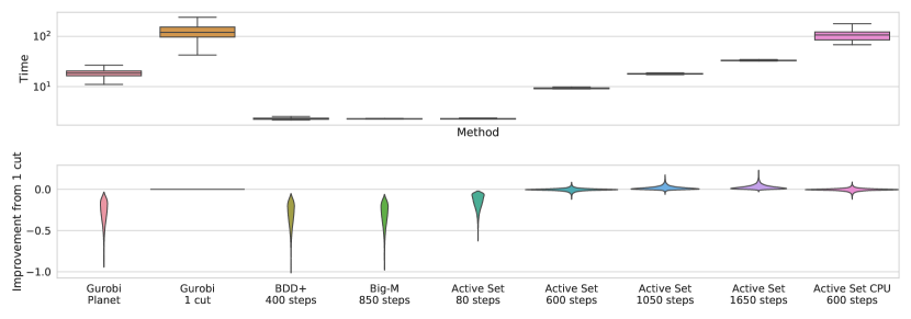
(a) Speed-accuracy trade-offs of Active Set for different iteration ranges and computing devices.

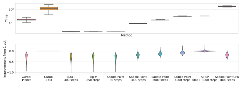
(b) Speed-accuracy trade-offs of Saddle Point for different iteration ranges and computing devices.

Figure 8: Robustness margin for the network adversarially trained with the method by  Madry et al. (2018), from Bunel et al. (2020a). Box plots: distribution of runtime in seconds. Violin plots: difference with the bounds obtained by Gurobi with a cut from $\mathcal{A}_{k}$ per neuron; higher is better, the width at a given value represents the proportion of problems for which this is the result.

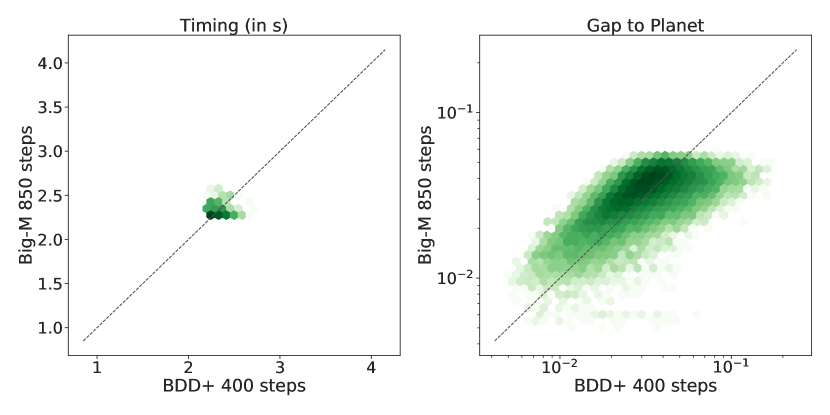
(a) Comparison of runtime (left) and gap to Gurobi Planet bounds (right). For the latter, lower is better.

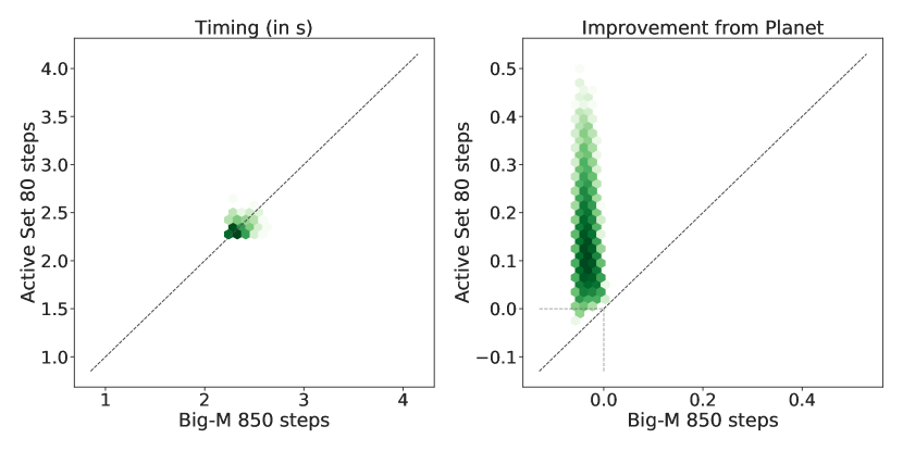
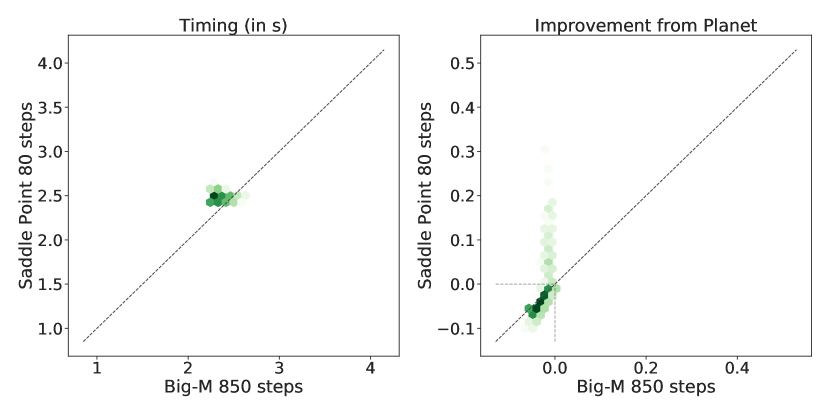
(b) Comparison of runtime (Timing) and difference with the Gurobi Planet bounds (Improvement from Planet). For the latter, higher is better.

Figure 9: Pointwise comparison for a subset of the methods on the data presented in figure 1. Darker colour shades mean higher point density (on a logarithmic scale). The oblique dotted line corresponds to the equality.

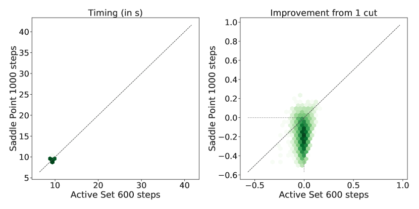
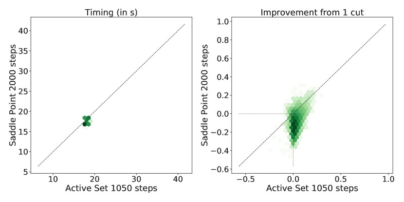
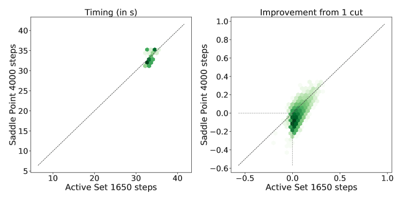
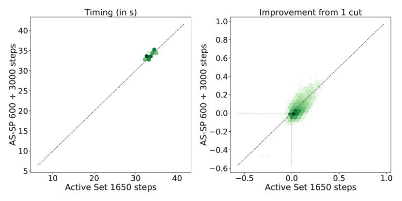
Figure 10: Pointwise comparison between our proposed solvers on the data presented in figure 8. Darker colour shades mean higher point density (on a logarithmic scale). The oblique dotted line corresponds to the equality.

In addition to the SGD-trained network in $\S$8.2, we now present results relative to the same architecture, trained with the adversarial training method by  Madry et al. (2018) for robustness to perturbations of $\epsilon_{train}=8/255$. Each adversarial sample for the training was obtained using 50 steps of projected gradient descent. For this network, we measure the robustness margin to perturbations with $\epsilon_{ver}=12/255$. Hyper-parameters are kept to the values tuned on the SGD-trained network from section 8.2.

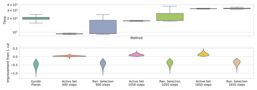
Figure 11: Upper plot: distribution of runtime in seconds. Lower plot: difference with the bounds obtained by Gurobi with a cut from $\mathcal{A}_{k}$ per neuron; higher is better. Results for the SGD-trained network from Bunel et al. (2020a). Sensitivity of Active Set to selection criterion (see $\S$4.2).

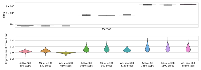
Figure 12: Upper plot: distribution of runtime in seconds. Lower plot: difference with the bounds obtained by Gurobi with a cut from $\mathcal{A}_{k}$ per neuron; higher is better. Results for the SGD-trained network from Bunel et al. (2020a). Sensitivity of Active Set to variable addition frequency $\omega$, with the selection criterion presented in $\S$4.2.

Figures 8, 9, 10 confirm most of the observations carried out for the SGD-trained network in $\S$8.2, with fewer variability around the bounds returned by Gurobi cut. Big-M is competitive with BDD+, and switching to Active Set after $500$ iterations results in much better bounds in the same time. Increasing the computational budget for Active Set still results in better bounds than Gurobi cut in a fraction of its running time, even though the performance gap is on average smaller than on the SGD-trained network. As in section 8.2 the gap between Saddle Point and Active Set, though larger here on average, decreases with the computational budget, and is further reduced when initializing with a few Active Set iterations.

H.2 Sensitivity of Active Set to selection criterion and frequency

In section 4.2, we describe how to iteratively modify $\mathcal{B}$, the active set of dual variables on which our Active Set solver operates. In short, Active Set adds the variables corresponding to the output of oracle (4) invoked at the primal minimiser of $\mathcal{L}_{\mathcal{B}}(\mathbf{x},\mathbf{z},\bm{\alpha},\bm{\beta}_{\mathcal{B}})$, at a fixed frequency $\omega$. We now investigate the empirical sensitivity of Active Set to both the selection criterion and the frequency of addition.

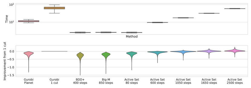
(a) Speed-accuracy trade-offs of Active Set for different iteration ranges and computing devices.

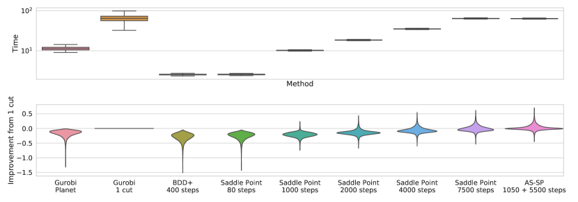
(b) Speed-accuracy trade-offs of Saddle Point for different iteration ranges and computing devices.

Figure 13: Robustness margin for the MNIST network adversarially trained with the method by  Wong and Kolter (2018), from Lu and Kumar (2020). Box plots: distribution of runtime in seconds. Violin plots: difference with the bounds obtained by Gurobi with a cut from $\mathcal{A}_{k}$ per neuron; higher is better.

We test against Ran. Selection, a version of Active Set for which the variables to add are selected at random by uniformly sampling from the binary $I_{k}$ masks. As expected, Figure 11 shows that a good selection criterion is key to the efficiency of Active Set. In fact, random variable selection only marginally improves upon the Planet relaxation bounds, whereas the improvement becomes significant with our selection criterion from $\S$4.2.

In addition, we investigate the sensitivity of Active Set (AS) to variable addition frequency $\omega$. In order to do so, we cap the maximum number of cuts at $7$ for all runs, and vary $\omega$ while keeping the time budget fixed (we test on three different time budgets). Figure 12 compares the results for $\omega=450$ (Active Set), which were presented in $\S$8.2, with the bounds obtained by setting $\omega=300$ and $\omega=600$ (respectively AS $\bm{\omega=300}$ and AS $\bm{\omega=600}$). Our solver proves to be relatively robust to $\omega$ across all the three budgets, with the difference in obtained bounds decreasing with the number of iterations. Moreover, early cut addition tends to yield better bounds in the same time, suggesting that our selection criterion is effective before subproblem convergence.

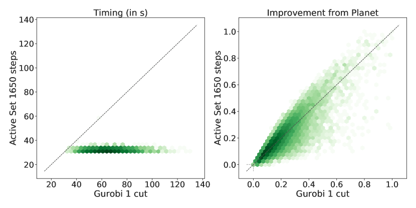
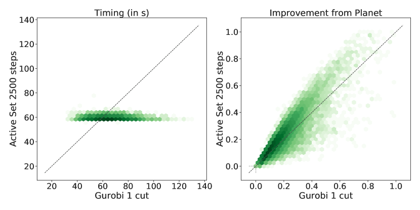
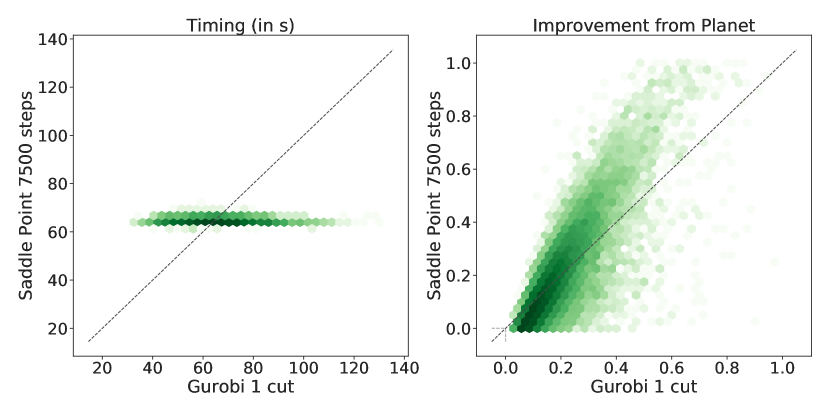
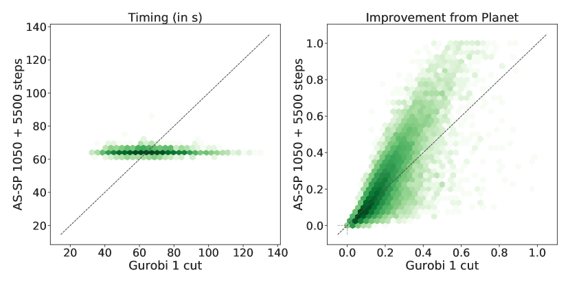
Figure 14: Pointwise comparison for a subset of the methods on the data presented in Figure 13. Comparison of runtime (left) and improvement from the Gurobi Planet bounds. For the latter, higher is better. Darker colour shades mean higher point density (on a logarithmic scale). The oblique dotted line corresponds to the equality.

H.3 MNIST Incomplete Verification

We conclude the experimental appendix by presenting incomplete verification results (the experimental setup mirrors the one employed in section 8.2 and appendix H.1) on the MNIST dataset (LeCun et al., 1998).

We report results on the “wide” MNIST network from Lu and Kumar (2020), whose architecture is identical to the “wide” network in Table 1 except for the first layer, which has only one input channel to reflect the MNIST specification (the total number of ReLU activation units is $4804$). As those employed for the complete verification experiments ($\S$8.3), and differently from the incomplete verification experiments in section 8.2 and appendix H.1, the network was adversarially trained with the method by Wong and Kolter (2018). We compute the robustness margin to $\epsilon_{ver}=0.15$ on the first $820$ images of the MNIST test set. All hyper-parameters are kept to the values employed for the CIFAR-10 networks, except the Big-M step size, which was linearly decreased from $10^{-1}$ to $10^{-3}$, and the weight of the proximal terms for BDD+, which was linearly increased from $1$ to $50$.

As seen on the CIFAR-10 networks, Figures 13, 14 show that our solvers for problem (3) (Active Set and Saddle Point) yield comparable or better bounds than Gurobi 1 cut in less average runtime. However, more iterations are required to reach the same relative bound improvement over Gurobi 1 cut (for Active Set, $2500$ as opposed to $600$ in Figures 1, 8). Finally, the smaller average gap between the bounds of Gurobi Planet and Gurobi 1 cut (especially with respect to Figure 1) suggests that the relaxation by Anderson et al. (2020) is less effective on this MNIST benchmark.

References

- Anderson et al. (2019) Ross Anderson, Joey Huchette, Christian Tjandraatmadja, and Juan Pablo Vielma. Strong mixed-integer programming formulations for trained neural networks. Conference on Integer Programming and Combinatorial Optimization, 2019.
- Anderson et al. (2020) Ross Anderson, Joey Huchette, Will Ma, Christian Tjandraatmadja, and Juan Pablo Vielma. Strong mixed-integer programming formulations for trained neural networks. Mathematical Programming, 2020.
- Balunovic and Vechev (2020) Mislav Balunovic and Martin Vechev. Adversarial training and provable defenses: Bridging the gap. 2020.
- Botoeva et al. (2020) Elena Botoeva, Panagiotis Kouvaros, Jan Kronqvist, Alessio Lomuscio, and Ruth Misener. Efficient verification of ReLU-based neural networks via dependency analysis. AAAI Conference on Artificial Intelligence, 2020.
- Bunel et al. (2018) Rudy Bunel, Ilker Turkaslan, Philip HS Torr, Pushmeet Kohli, and M Pawan Kumar. A unified view of piecewise linear neural network verification. Neural Information Processing Systems, 2018.
- Bunel et al. (2020a) Rudy Bunel, Alessandro De Palma, Alban Desmaison, Krishnamurthy Dvijotham, Pushmeet Kohli, Philip HS Torr, and M Pawan Kumar. Lagrangian decomposition for neural network verification. Conference on Uncertainty in Artificial Intelligence, 2020a.
- Bunel et al. (2020b) Rudy Bunel, Jingyue Lu, Ilker Turkaslan, P Kohli, P Torr, and M Pawan Kumar. Branch and bound for piecewise linear neural network verification. Journal of Machine Learning Research, 21(2020), 2020b.
- Candès et al. (2008) Emmanuel J. Candès, Michael B. Wakin, and Stephen P. Boyd. Enhancing sparsity by reweighted 1 minimization. Journal of Fourier Analysis and Applications, 2008.
- Carlini and Wagner (2017) Nicholas Carlini and David Wagner. Towards evaluating the robustness of neural networks. 2017 IEEE Symposium on Security and Privacy, 2017.
- De Palma et al. (2021) Alessandro De Palma, Harkirat Singh Behl, Rudy Bunel, Philip H. S. Torr, and M. Pawan Kumar. Scaling the convex barrier with active sets. International Conference on Learning Representations, 2021.
- Dvijotham et al. (2018) Krishnamurthy Dvijotham, Robert Stanforth, Sven Gowal, Timothy Mann, and Pushmeet Kohli. A dual approach to scalable verification of deep networks. Uncertainty in Artificial Intelligence, 2018.
- Dvijotham et al. (2019) Krishnamurthy Dvijotham, Robert Stanforth, Sven Gowal, Chongli Qin, Soham De, and Pushmeet Kohli. Efficient neural network verification with exactness characterization. Uncertainty in Artificial Intelligence, 2019.
- Ehlers (2017) Ruediger Ehlers. Formal verification of piece-wise linear feed-forward neural networks. Automated Technology for Verification and Analysis, 2017.
- Frank and Wolfe (1956) Marguerite Frank and Philip Wolfe. An algorithm for quadratic programming. Naval Research Logistics Quarterly, 1956.
- Gidel et al. (2017) Gauthier Gidel, Tony Jebara, and Simon Lacoste-Julien. Frank-Wolfe algorithms for saddle point problems. In Proceedings of the 20th International Conference on Artificial Intelligence and Statistics, 2017.
- Gowal et al. (2018) Sven Gowal, Krishnamurthy Dvijotham, Robert Stanforth, Rudy Bunel, Chongli Qin, Jonathan Uesato, Timothy Mann, and Pushmeet Kohli. On the effectiveness of interval bound propagation for training verifiably robust models. SECML NeurIPS, 2018.
- Gurobi Optimization (2020) LLC Gurobi Optimization. Gurobi optimizer reference manual, 2020. URL http://www.gurobi.com.
- Jaggi (2013) Martin Jaggi. Revisiting Frank-Wolfe: Projection-free sparse convex optimization. International Conference on Machine Learning, 2013.
- Jeroslow (1987) R. G. Jeroslow. Representability in mixed integer programming, i: Characterization results. Discrete Applied Mathematics, 1987.
- Katz et al. (2017) Guy Katz, Clark Barrett, David Dill, Kyle Julian, and Mykel Kochenderfer. Reluplex: An efficient SMT solver for verifying deep neural networks. International Conference on Computer-Aided Verification, 2017.
- Kingma and Ba (2015) Diederik P. Kingma and Jimmy Ba. Adam: A method for stochastic optimization. International Conference on Learning Representations, 2015.
- Krizhevsky and Hinton (2009) A. Krizhevsky and G. Hinton. Learning multiple layers of features from tiny images. Master’s thesis, Department of Computer Science, University of Toronto, 2009.
- Kurakin et al. (2017) Alexey Kurakin, Ian J. Goodfellow, and Samy Bengio. Adversarial machine learning at scale. International Conference on Learning Representations, 2017.
- LeCun et al. (1998) Yann LeCun, Léon Bottou, Yoshua Bengio, and Patrick Haffner. Gradient-based learning applied to document recognition. IEEE, 1998.
- Lemaréchal (2001) Claude Lemaréchal. Lagrangian relaxation. In Computational combinatorial optimization, pages 112–156. Springer, 2001.
- Lu and Kumar (2020) Jingyue Lu and M Pawan Kumar. Neural network branching for neural network verification. In International Conference on Learning Representations, 2020.
- Madry et al. (2018) Aleksander Madry, Aleksandar Makelov, Ludwig Schmidt, Dimitris Tsipras, and Adrian Vladu. Towards deep learning models resistant to adversarial attacks. International Conference on Learning Representations, 2018.
- Paszke et al. (2017) Adam Paszke, Sam Gross, Soumith Chintala, Gregory Chanan, Edward Yang, Zachary DeVito, Zeming Lin, Alban Desmaison, Luca Antiga, and Adam Lerer. Automatic differentiation in pytorch. NIPS Autodiff Workshop, 2017.
- Raghunathan et al. (2018) Aditi Raghunathan, Jacob Steinhardt, and Percy S Liang. Semidefinite relaxations for certifying robustness to adversarial examples. Neural Information Processing Systems, 2018.
- Salman et al. (2019) Hadi Salman, Greg Yang, Huan Zhang, Cho-Jui Hsieh, and Pengchuan Zhang. A convex relaxation barrier to tight robustness verification of neural networks. Neural Information Processing Systems, 2019.
- Sherali and Choi (1996) Hanif D. Sherali and Gyunghyun Choi. Recovery of primal solutions when using subgradient optimization methods to solve lagrangian duals of linear programs. Operations Research Letters, 1996.
- Singh et al. (2018) Gagandeep Singh, Timon Gehr, Matthew Mirman, Markus Püschel, and Martin Vechev. Fast and effective robustness certification. Neural Information Processing Systems, 2018.
- Singh et al. (2019a) Gagandeep Singh, Rupanshu Ganvir, Markus Püschel, and Martin Vechev. Beyond the single neuron convex barrier for neural network certification. Neural Information Processing Systems, 2019a.
- Singh et al. (2019b) Gagandeep Singh, Timon Gehr, Markus Püschel, and Martin Vechev. Boosting robustness certification of neural networks. International Conference on Learning Representations, 2019b.
- Singh et al. (2020) Gagandeep Singh, Jonathan Maurer, Christoph Müller, Matthew Mirman, Timon Gehr, Adrian Hoffmann, Petar Tsankov, Dana Drachsler Cohen, Markus Püschel, and Martin Vechev. ETH robustness analyzer for neural networks (ERAN), 2020. URL https://github.com/eth-sri/eran.
- Szegedy et al. (2014) Christian Szegedy, Wojciech Zaremba, Ilya Sutskever, Joan Bruna, Dumitru Erhan, Ian Goodfellow, and Rob Fergus. Intriguing properties of neural networks. International Conference on Learning Representations, 2014.
- Tjandraatmadja et al. (2020) Christian Tjandraatmadja, Ross Anderson, Joey Huchette, Will Ma, Krunal Patel, and Juan Pablo Vielma. The convex relaxation barrier, revisited: Tightened single-neuron relaxations for neural network verification. arXiv preprint arXiv:2006.14076, 2020.
- Tjeng et al. (2019) Vincent Tjeng, Kai Xiao, and Russ Tedrake. Evaluating robustness of neural networks with mixed integer programming. International Conference on Learning Representations, 2019.
- VNN-COMP (2020) VNN-COMP. International verification of neural networks competition (VNN-COMP). Verification of Neural Networks workshop at the International Conference on Computer-Aided Verification, 2020. URL https://sites.google.com/view/vnn20/vnncomp.
- Wang et al. (2018) Shiqi Wang, Kexin Pei, Justin Whitehouse, Junfeng Yang, and Suman Jana. Efficient formal safety analysis of neural networks. Neural Information Processing Systems, 2018.
- Webb et al. (2019) Stefan Webb, Tom Rainforth, Yee Whye Teh, and M Pawan Kumar. A statistical approach to assessing neural network robustness. International Conference on Learning Representations, 2019.
- Weng et al. (2018) Tsui-Wei Weng, Huan Zhang, Hongge Chen, Zhao Song, Cho-Jui Hsieh, Duane Boning, Inderjit S Dhillon, and Luca Daniel. Towards fast computation of certified robustness for relu networks. International Conference on Machine Learning, 2018.
- Wong and Kolter (2018) Eric Wong and Zico Kolter. Provable defenses against adversarial examples via the convex outer adversarial polytope. International Conference on Machine Learning, 2018.