Agglomerative Hierarchical Clustering for Selecting Valid Instrumental Variables

Abstract

We propose a procedure, which combines hierarchical clustering with a test of overidentifying restrictions for selecting valid instrumental variables (IV) from a large set of IVs. Some of these may be invalid in that they fail the exclusion restriction. We show that if the largest group of IVs is valid, our method achieves oracle properties. Unlike existing techniques, our work deals with multiple endogenous regressors, weak instruments, heterogeneous effects and near validity. In simulations our procedure outperforms the Hard Thresholding and the Confidence Interval method. The method is applied to estimating the effect of immigration on wages and the return to education.

Keywords: Causal inference, Cluster Analysis, Instrumental variables, Invalid Instruments

1 Introduction

Instrumental variables estimation is a widely used statistical method for analysing the causal effects of treatment variables on an outcome when the causal relationship between them is confounded. Consistent IV estimation requires that all instruments are valid. This requires that

1. Instruments are associated with the endogenous variables (relevance condition)

2. Instruments do not affect the outcome directly or through unobserved factors (exclusion restriction)

In practice, a main challenge in IV estimation is that some instrumental variables may be invalid in the sense that they fail the exclusion restriction. The key task therefore is to estimate the causal effect in situations where the number of IVs is large.

In this paper, we propose a new method to select the valid instruments and to estimate the causal effect. The method combines the agglomerative hierarchical clustering (AHC) algorithm, a statistical learning algorithm typically employed in cluster analysis, with the Sargan test for overidentifying restrictions. The estimator that we develop relies on the plurality rule [17] which states that the largest group of IVs consists of valid instruments. Instruments are said to form a group if their instrument-specific just-identified estimators converge to the same value. Under the plurality rule, our method achieves oracle selection. This means that the estimator works as well as if the set of true instruments were known: valid instruments can be selected consistently, and the two-stage least squares (2SLS) estimator using the instruments selected as valid has the same limiting distribution as the ideal estimator that uses the set of truly valid instruments.

Our work adds to a growing literature on valid IV selection inspired by [4] who proposes moment selection criteria and a downward testing procedure. The setting considered in this literature is one where the number of IVs is large in the sense that the number of IVs by far exceeds the number of regressors and considering all possible overidentified models becomes infeasible. However, we are not in a setting where the number of instruments grows with the number of observations. The literature we relate to is also different from the one that uses regularization to find an optimal set of instruments, as in [8] in that it does not uphold the assumption that all IVs fulfil the violation restriction.

Our method improves upon the existing methods in that it is the first to allow for multiple endogenous regressors, deal with weak instruments without calling for a first-stage selection, and accommodate heterogeneous effects and combinations of these. Moreover, it outperforms the existing methods in simulations.

A prominent example for a setting with a large number of IVs, all of which have to be valid is the estimation of the effect of immigration on wages in labor economics. To identify causal effects, researchers often rely on the lagged origin-country specific immigration pattern, measured by previous shares of immigrants. If none of the previous shares by origin country are directly or indirectly correlated with the outcome variable, the causal effect can be consistently estimated. This assumption is invoked very often in the literature. However, some of the shares may violate the exclusion restrictions, as they may affect the wage variable directly through long-term dynamic adjustment processes, or be correlated with unobserved demand shocks.

Another example where a large number of instruments are present is the estimation of the return to education. Here, interactions of quarter- and year-fixed effects have been famously used by [5]. These IVs have been shown to suffer from a weak instrument problem by [9]. In this context, our method might be helpful in selecting IVs which are strong and valid.

Another field that makes use of a large number of instruments, some of which may be invalid is Mendelian Randomization. Here, researchers use genetic variation to estimate the causal effect of an exposure on a health-related outcome. This field has also inspired much of the initial invalid IV selection literature. An example is the estimation of the effect of C-reactive protein on coronary heart disease [27].

In the applied literature, the two solutions used most often are to select valid instruments from the set of potential instruments based on economic intuition, or to directly include all the candidate instruments in IV estimation. These approaches can be problematic because including invalid instruments often leads to severely biased results. Therefore, it is important to develop data-driven IV selection methods to select invalid instruments, when complete knowledge about the candidate instruments’ validity is absent.

Previous work has tackled the IV selection problem in the single endogenous variable case. [22] propose a selection method based on the least absolute shrinkage and selection operator (LASSO). [30] make improvements by proposing an adaptive Lasso based method that has oracle properties under the assumption that more than half of the candidate instruments are valid (the majority rule). [17] propose the Hard Thresholding with Voting method (HT) that has oracle properties under the sufficient and necessary identification condition that the largest group is formed by all the valid instruments (the plurality rule). This is a relaxation to the majority rule. Under the same identification condition, [31] propose the Confidence Interval method (CIM), which has better finite sample performance.

Our research adds to the literature in five ways:

1. We combine agglomerative hierarchical clustering with a traditional statistical test, the Sargan over-identification test, to yield a novel downward testing algorithm for IV selection. This new method provides the theoretical guarantee that under the plurality rule it can select the true set of valid instruments consistently, and is computationally feasible.

2. We extend the method to settings with multiple endogenous regressors. Such an extension is not available for the aforementioned methods, but it is straightforward in our setting.

3. Our method performs well in the presence of weak valid or invalid instruments, which is an advantage over existing methods.

4. We also discuss the application of our method to a setting with heterogeneous treatment effects. Importantly, we can retrieve and inspect the entire group structure, a possibility that the previous methods do not offer.

5. Our algorithm is computationally less complex than the CI and HT methods. Also, the only pre-specified parameter for our algorithm is the critical value for the Sargan test, which has been well established in the existing literature to guarantee consistent selection.

We also discuss implications in settings with local-to-zero violations of the exclusion restriction. We conduct Monte Carlo simulations to examine the performance of our method, and compare it with two existing methods: the Hard Thresholding method and the Confidence Interval method. We compare with these two methods, because they also rely on the plurality rule. The simulation results show that our method achieves oracle performance in both single and multiple endogenous regressors settings in large samples when all the instruments are strong. Also, our method works well when some of the candidate instruments are weak, outperforming HT and CIM.

We illustrate the various strength of our method with two illustrations. We apply our method to the estimation of the short- and long-run effects of immigration on wages in the US by reproducing and revisiting the results of [7]. In this example, we have two endogenous regressors, potentially weak and invalid instruments. The results of [5] on the returns to education are also revisited. Here, the main concern is that instruments are weak. In both applications our estimator indicate that the actual effects might be much larger than suggested by the standard 2SLS estimates. In particular for the second application, the first-stage F-statistic doubles after preselection via AHC. We also provide an R-package that makes implementation of our method easy in practice.

The remainder of this paper is structured as follows. In Section 2, we state the model and assumptions and illustrate some of the well-established properties of the 2SLS just-identified estimator. In Section 3, we describe the basic method and the algorithm when there is a single endogenous variable, and investigate its asymptotic properties. In Section 4, we present extensions to settings with multiple endogenous regressors and weak instruments, and discuss our method in presence of heterogeneous treatment effects. In Section 5, we provide Monte Carlo simulation results. In Section 6, we apply our method to estimate the effects of immigration on wages and to the returns to education and add a discussion of how our method could be applied to the estimation of the effect of pollutants on human health. Section 7 concludes.

2 Model and Assumptions

In the following, we introduce notational conventions used throughout this paper. Matrices are in upper case and bold. Vectors are in lower case and bold. Scalars are in lower case and not in bold. Let $\mathbf{y}$ be an $n\times 1$-vector of the observed outcome, $\mathbf{d}_{1}$, …, $\mathbf{d}_{P}$ be $P$ endogenous regressor vectors (each $n\times 1$), which can be subsumed in an $n\times P$ - matrix $\mathbf{D}$, $\mathbf{z}_{1}$, …, $\mathbf{z}_{J}$ be $J$ instrument vectors, which can be subsumed in an $n\times J$ - matrix $\mathbf{Z}$. Let error terms be $\mathbf{u}$ and $\bm{\varepsilon_{p}}$ for $p\in\{1,...,P\}$, which are all $n\times 1$ error-vectors and are correlated with $\sigma_{up}:=cov(\mathbf{u},\bm{\varepsilon}_{p})$. The latter covariances measure the endogeneity of regressors in $\mathbf{D}$. The $P\times 1$ coefficient vector of interest is $\bm{\beta}$. The $J\times P$ matrix $\bm{\gamma}$ contains first-stage coefficients. Let $s$ be the number of instruments in the set of valid instruments, $\mathcal{I}$, $g$ be the number of instruments in the set of invalid instruments, $\mathcal{V}$, and $J=g+s$ be the total number of instruments in the overall set of instruments, $\mathcal{J}$. The arithmetic mean of a variable $x$ is defined as $\mu_{x}=\frac{\Sigma_{i=1}^{n}x_{i}}{n}$, the mean of a vector is the vector of dimension-wise arithmetic means, $\lVert\cdot\rVert$ denotes the L2-norm and $|\cdot|$ denotes cardinality, when used around a set and an absolute value, when used around a quantity. The symbol $\&$ denotes the logical conjunction, and. The $n\times n$ projection matrix is $\mathbf{P}_{X}=\mathbf{X}(\mathbf{X}^{\prime}\mathbf{X})^{-1}\mathbf{X}^{\prime}$, and the annihilator matrix is $\mathbf{M}_{X}=\mathbf{I}-\mathbf{P}_{X}$ and $\hat{\mathbf{D}}=\mathbf{P}_{Z}\mathbf{D}$ are the fitted values. Throughout the paper, we assume that $J$, $Q$ and $g$ are fixed and $P<J$.

2.1 Model Setup

We start from the model setup with a single endogenous regressor, i.e. throughout Section 2 and Section 3, $P=1$. The extension of our method to the cases with multiple endogenous regressors can be found in Section 4.1. All proofs in the Appendix are for a general $P$.

We adopt the following observed data model which takes the potentially invalid instruments into account:

$$\mathbf{y}=\mathbf{d}\beta+\mathbf{Z}\bm{\alpha}+\mathbf{u}\text{,}$$ (1)

with $\mathbf{E}[u_{i}|\mathbf{z}_{i}]=0$. The linear projection of $\mathbf{d}$ on $\mathbf{Z}$ is

$$\mathbf{d}=\mathbf{Z}\bm{\gamma}+\bm{\varepsilon}$$ (2)

The vector $\bm{\alpha}$ is $J\times 1$ and has entries $\alpha_{j}$, each of which is associated with an individual instrument. Each entry indicates which of the instruments has a direct effect on the outcome variable and hence is invalid. Following a large econometric and statistical literature, such as [23], [11], [17] or [22], we define a valid instrument as:

Definition 1.

For $j=1,...,J$, instrument $\mathbf{z}_{j}$ is valid if $\alpha_{j}=0$. If $\alpha_{j}\neq 0$, then $\mathbf{z}_{j}$ is an invalid instrument.

Following the cited literature, we restrict our attention to violations of the exclusion restriction. This could be extended to violations of exogeneity, as in $Cov(\mathbf{Z},\mathbf{e})\neq 0$, where $\mathbf{e}=\mathbf{\mathbf{Z}\bm{\alpha}+\mathbf{u}}$. The consequences of this important conceptual difference are however beyond the scope of this paper and we leave it to future work.

The ideal model which selects the truly valid instruments as valid and controls for the set of invalid instruments is the oracle model, defined as follows:

$$\mathbf{y}=\mathbf{d}\beta+\mathbf{Z}_{\mathcal{I}}\bm{\alpha}_{\mathcal{I}}+\mathbf{u}=\mathbf{X}_{\mathcal{I}}\bm{\theta}_{\mathcal{I}}+\mathbf{u}\text{.}$$ (3)

where $\mathbf{X}_{\mathcal{I}}=(\mathbf{d}\quad\mathbf{Z}_{\mathcal{I}})$ and $\bm{\theta}_{\mathcal{I}}=(\beta\quad\bm{\alpha}_{\mathcal{I}}^{\prime})^{\prime}$.

2.2 Assumptions

The assumptions that follow are the same as in [31]. The first assumption is a rank assumption.

Assumption 1.

Rank assumption.

$$E(\mathbf{z}_{i}\mathbf{z}_{i}^{\prime})=\mathbf{Q}\text{ with }\mathbf{Q}\text{ a finite and full rank matrix.}$$

The second assumption makes sure that the just-identified estimators all exist.

Assumption 2.

Existence of just-identified estimators.

$$\bm{\gamma}=(E[\mathbf{z}_{i}\mathbf{z}_{i}^{\prime}])^{-1}E[\mathbf{z}_{i}d_{i}]),\gamma_{j}\neq 0\quad j=1,...,J\textbf{.}$$

Assumption 3.

Error structure.
Let $\mathbf{w}_{i}=(u_{i}\quad\varepsilon_{i})^{\prime}$. Then, $E(\mathbf{w}_{i})=0$ and $E[\mathbf{w}_{i}\mathbf{w}_{i}^{\prime}]=\left(\begin{array}[]{rr}\sigma_{u}^{2}&\sigma_{u,\varepsilon}\\ \sigma_{u,\varepsilon}&\sigma_{\varepsilon}^{2}\end{array}\right)=\bm{\Sigma}$ with
$Var(u_{i})=\sigma_{u}^{2},\quad Var(\varepsilon_{i})=\sigma_{\varepsilon}^{2}\quad Cov(u_{i},\varepsilon_{i})=\sigma_{u,\varepsilon}$ and the elements of $\bm{\Sigma}$ are finite.

Assumption 4.

$$plim(n^{-1}\mathbf{Z}^{\prime}\mathbf{Z})=E(\mathbf{z}_{i}\mathbf{z}_{i}^{\prime})=\mathbf{Q}\quad ;\quad plim(n^{-1}\mathbf{Z}^{\prime}\mathbf{d})=E(\mathbf{z}_{i}d_{i})$$

$$plim(n^{-1}\mathbf{Z}^{\prime}\bm{u})=E(\mathbf{z}_{i}u_{i})=0\quad ;\quad plim(n^{-1}\mathbf{Z}^{\prime}\bm{\varepsilon})=E(\mathbf{z}_{i}\varepsilon_{i})=0$$

$$plim(n^{-1}\sum\limits_{i=1}^{n}\mathbf{w}_{i})=0\quad ;\quad plim(n^{-1}\mathbf{w}_{i}\mathbf{w}_{i}^{\prime})=\bm{\Sigma}\text{.}$$

Assumption 5.

$\frac{1}{\sqrt{n}}\sum\limits_{i=1}^{n}vec(\mathbf{z}_{i}\mathbf{w}_{i}^{\prime})\overset{d}{\rightarrow}N(0,\bm{\Sigma\otimes\mathbf{Q}})\text{ as }n\rightarrow\infty$.

The assumptions above will be modified when there is more than one endogenous regressor. Assumption 5 is made for ease of exposition, but the method can be easily extended to accommodate heteroskedasticity, clustering and serial correlation. From $(1)$ and $(2)$, we have the outcome-instrument reduced form

$$\mathbf{y}=\mathbf{Z}\bm{\Gamma}+\bm{\epsilon}$$

where $\Gamma_{j}=\gamma_{j}\beta+\alpha_{j}$. Each individual instrument $\mathbf{z}_{j}$ is associated with a just-identified estimator for $\beta$, denoted by $\hat{\beta}_{j}$, which is defined as the two-stage least squares (2SLS) estimator using $\mathbf{z}_{j}$ as the single valid instruments, and treating the remaining IVs as controls. There are $J$ just-identified IV estimators. We write these estimators as in [31].

$$\hat{\beta}_{j}=\frac{\hat{\Gamma}_{j}}{\hat{\gamma}_{j}}$$

where $\hat{\Gamma}_{j}$ and $\hat{\gamma}_{j}$ are the OLS estimators for $\Gamma_{j}$ and $\gamma_{j}$ respectively. Then we have

Property 1.

Properties of just-identified estimates.
Under Assumptions 2 to 5 it holds that

$$plim(\hat{\beta}_{j})=plim\left(\frac{\hat{\Gamma}_{j}}{\hat{\gamma}_{j}}\right)=\beta+\frac{\alpha_{j}}{\gamma_{j}}$$

Hence, the inconsistency of $\hat{\beta}_{j}$ is $plim(\hat{\beta}_{j})-\beta=\frac{\alpha_{j}}{\gamma_{j}}=q$. We define a group following the definition in [17] as:

Definition 2.

A group $\mathcal{G}_{q}$ is a set of IVs that has the same estimand $\beta_{j}=\beta+q$.

$$\mathcal{G}_{q}=\{j:\beta_{j}=\beta+q\}$$

Then the group consisting of all valid instruments is

$$\mathcal{G}_{0}=\{j:q=0\}$$

Let the number of groups be $Q$, which is finite because the number of IVs $J$ is also finite.

The next assumption is the key assumption for identification. It states that among the $Q$ groups formed by $\mathbf{z}_{1},...,\mathbf{z}_{J}$, the largest group is composed by all the valid IVs. A group is defined as above, as a set of instruments whose just-identified estimators converge to the same value $\beta+q$.

Assumption 6.

Plurality Rule.

$$g>\underset{q\neq 0}{max}|\mathcal{G}_{q}|$$

3 IV Selection and Estimation Method

Based on the definition of groups and the plurality rule, a natural strategy for IV selection is to find out the $Q$ IV groups and then select the largest group as the set of valid instruments. In this paper, we explore the clustering methods to discover the IV groups. First, we fit the general clustering framework to the IV selection problem, which is summarized in the minimisation problem in 4. This general method needs a pre-specified parameter $K$, which is the number of clusters. We show that when $K$ equals the number of groups, there is a unique solution to this minimization problem. This solution coincides with the true underlying partition. However, the fact that consistent selection depends on $K$ makes it difficult to implement in practice, as we do not have prior knowledge about the number of groups. If $K$ is too large (larger than the number of groups), then the largest group will be split. If $K$ is too small, then the largest group might be in a cluster with some other group. To tackle this problem, we propose a downward testing procedure which combines the agglomerative hierarchical clustering method (Ward’s method) with the Sargan test for overidentifying restrictions to select the valid instruments, which allows us to select the valid instruments without pre-specifying $K$.

3.1 Clustering Method for IV Selection

Let $\mathbf{\mathcal{S}}=\{\mathcal{S}_{1},...,\mathcal{S}_{K}\}$ be a partition of $J$ just-identified estimators $\hat{\beta}_{j}$ into $K$ cluster cells with cluster identities $k=1,...,K$. The clustering result is the solution to the following minimization problem:

$$\mathbf{\hat{\mathcal{S}}}(K)=\underset{\mathbf{\mathcal{S}}}{\operatorname*{argmin}}\sum_{k=1}^{K}\sum_{\hat{\beta}_{j}\in\mathcal{S}_{k}}||\hat{\beta}_{j}-\bar{\mathcal{S}}_{k}||^{2}\text{,}$$ (4)

where $\bar{\mathcal{S}}_{k}$ is the arithmetic mean of all just-identified estimators in cluster $\mathcal{S}_{k}$. This corresponds to the intra-cluster variance, summed over the number of clusters.
Let the clustering result $\hat{\mathcal{S}}(K)$ be an estimator of sets containing IV-estimators $\hat{\beta_{j}}$. The IV-estimators in a cluster $\hat{\mathcal{S}}_{k}$ are selected to belong to a certain group of IVs:

$$\hat{\mathcal{G}}_{k}=\{j:\hat{\beta}_{j}\in\hat{\mathcal{S}}_{k}\}$$

Based on Assumption 6, the cluster that consists of estimators that use valid IVs is estimated as the cluster that contains the largest number of just-identified estimators:

$$\hat{\mathcal{S}}_{m}(K)=\{\mathcal{S}(K):|\hat{\mathcal{S}}(K)|=\underset{k}{max}|\hat{\mathcal{S}}_{k}(K)|\}$$

The valid IVs are selected as those IVs that are used to estimate the largest cluster $\hat{\mathcal{S}}_{m}(K)$

$$\hat{\mathcal{V}}(K)=\{j:\hat{\beta}_{j}\in\hat{\mathcal{S}}_{m}(K)\}\text{.}$$

Then, the remaining IVs are selected as invalid

$$\hat{\mathcal{I}}(K)=\mathcal{J}\quad\backslash\quad\hat{\mathcal{V}}(K).$$

When the number of clusters $K$ is equal to the number of groups $Q$, $K=Q$, then there is a partition minimizing the sum in Equation 4. This occurs, when the grouping is such that $\mathcal{G}_{k}=\mathcal{G}_{q}$, i.e. each selected group $\mathcal{G}_{k}$ is in fact formed by a true group, $\mathcal{G}_{q}$. Define the partition leading to this grouping of IVs as the true partition $\mathbf{\mathcal{S}}_{0}=\{\mathcal{S}_{01},...,\mathcal{S}_{0Q}\}$.

To see that, first note that if the partition is such that $\hat{\mathcal{S}}_{k}=\mathcal{S}_{0q}\,\,\forall k,q$, i.e. $\hat{\mathbf{\mathcal{S}}}(K)=\mathbf{\mathcal{S}}_{0}$,

$$g(\hat{\mathbf{\mathcal{S}}}(K))=g(\mathbf{\mathcal{S}}_{0})=plim\{\sum_{k=1}^{K}\sum_{\hat{\beta}_{j}\in\mathcal{S}_{k}}||\hat{\beta}_{j}-\bar{\mathcal{S}}_{k}||^{2}\}=0\text{.}$$

For all $\hat{\beta}_{j}\in\mathcal{S}_{k}$, we have $plim\,\hat{\beta}_{j}=plim\,\bar{\mathcal{S}}_{k}$, and $plim\{||\hat{\beta}_{j}-\bar{\mathcal{S}}_{k}||^{2}\}=0$. This is the case for all $k\in 1,...K$, hence $g(\mathbf{\mathcal{S}}_{0})=0$. Second, if the partition is such that some $\mathcal{S}_{k}\neq\mathcal{S}_{0q}$, i.e. $\mathbf{\mathcal{S}}\neq\mathbf{\mathcal{S}}_{0}$, then $plim\,\hat{\beta}_{j}\neq plim\,\bar{\mathcal{S}}_{k}$ for some $\hat{\beta}_{j}\in\mathcal{S}_{k}$ and $g(\mathbf{\mathcal{S}})>0$. This means that when $n\rightarrow\infty$ there is a unique solution for Equation 4, which is such that $\mathbf{\mathcal{S}}=\mathbf{\mathcal{S}}_{0}$. A necessary condition for this to hold is that $K=Q$.

3.2 Ward’s Algorithm for IV Selection

To choose the correct value of $K$ without prior knowledge of the number of groups, we propose a selection method which combines Ward’s algorithm, a general agglomerative hierarchical clustering procedure proposed by [26], with the Sargan test of overidentifying restrictions. Our selection algorithm has two parts. The set of instruments selected as valid by the algorithm is denoted by $\hat{\mathcal{V}}^{dts}$.

The first part is Ward’s algorithm, as described in Algorithm 1 below. Ward’s algorithm aims to minimize the total within-cluster sum of squared error. This is achieved by minimizing the increase in within-cluster sum of squared error at each step of the algorithm. The method generates a path of cluster assignments with $K$ clusters at each step so that $K\in\{1,...,J\}$. After obtaining the clusters for each $K$, we use a downward testing procedure based on the Sargan-test to select the set of valid instruments (Algorithm 2).

Ward’s Algorithm works as follows

Algorithm 1.

Ward’s algorithm

1. Input: Each just-identified point estimate is calculated. The Euclidean distance between all of these estimates is calculated and written as a dissimilarity matrix.

2. Initialization: Each just-identified estimate has its own cluster. The total number of clusters in the beginning hence is $J$.

3. Joining: The two clusters which are closest as measured by their weighted squared Euclidean distance $\frac{|\mathcal{S}_{k}||\mathcal{S}_{l}|}{|\mathcal{S}_{k}|+|\mathcal{S}_{l}|}||\bar{\mathcal{S}}_{k}-\bar{\mathcal{S}}_{l}||^{2}$ are joined to a new cluster. $|\mathcal{S}_{k}|$ is the number of estimates in cluster $k$. $\bar{\mathcal{S}}_{k}$ denotes the mean of cluster $k$, which is the arithmetic mean of all the just-identified estimates in $\mathcal{S}_{k}$.

4. Iteration: The joining step is repeated until all just-identified point-estimates are in one cluster.

This yields a path of $S=J-1$ steps, on which there are clusters of size $K\in\{1,...,J\}$. [26] originally also allows for alternative objective functions. These are associated with different dissimilarity metrics and different ways to define the distance between clusters. Our motivation for using the Euclidean distance is that the objective function is the intra-cluster variance or the sum of residual sum of squares. We discuss alternative choices of these so-called linkage methods and dissimilarity metrics in Section 4.5.

After generating the clustering path by Algorithm 1, we select the set of valid instruments following Algorithm 2:

Algorithm 2.

Downward testing procedure

1. Starting from $K=1$, find the cluster that contains the largest number of just-identified estimators. In the first step, all estimators are in one cluster.

2. Do Sargan test on the instruments associated with the largest cluster, using the rest of IVs as controls. If there are multiple such clusters, select the one with the smallest Sargan statistic.

3. Repeat the procedure for each $K=2,...,J-1$.

4. Stop when for the first time, the model selected by the largest cluster at some $K$ does not get rejected by the Sargan test.

5. Select the instruments associated with the cluster from Step 4 as valid instruments.

The Sargan statistic in Step 4 is given by

$$Sar\left(K\right)=\frac{\widehat{\mathbf{u}}(\widehat{\bm{\theta}}_{K})^{\prime}\mathbf{Z}\left(\mathbf{Z}^{\prime}\mathbf{Z}\right)^{-1}\mathbf{Z}^{\prime}\widehat{\mathbf{u}}(\widehat{\bm{\theta}}_{K})}{\widehat{\mathbf{u}}(\widehat{\bm{\theta}}_{K})^{\prime}\widehat{\mathbf{u}}(\widehat{\bm{\theta}}_{K})/n}$$

where $\hat{\bm{\theta}}_{K}$ is the 2SLS estimator using the instruments associated with the largest cluster for each $K$ as valid instruments and controlling for the rest of the instruments, and $\widehat{\mathbf{u}}(\widehat{\bm{\theta}}_{K})$ is the 2SLS residual. We show later that to guarantee consistent selection, the critical value for the Sargan test, denoted by $\xi_{n,J-|\hat{\mathcal{I}}|-P}$ should satisfy $\xi_{n,J-|\hat{\mathcal{I}}|-P}\rightarrow\infty$ and $\xi_{n,J-|\hat{\mathcal{I}}|-P}=o(n)$. In practice, we choose the significance level $\frac{0.1}{log(n)}$ following [31].

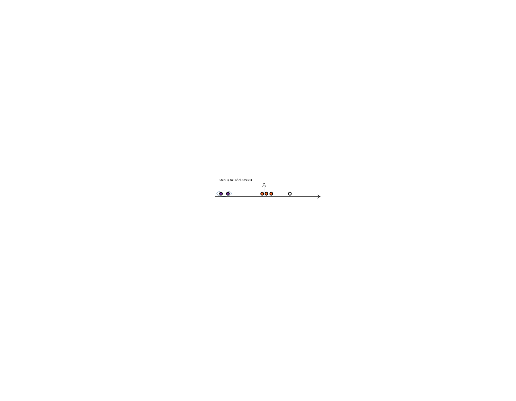
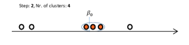
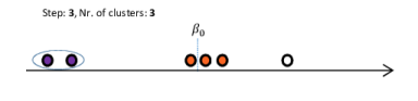
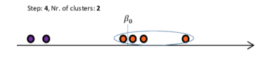
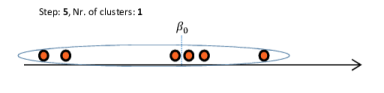
Figure 1: Illustration of the Algorithm with One Regressor

The procedure is illustrated in figure 1. Here, we have a situation with six instruments. Three of them are valid as they affect the outcome variable only through the endogenous regressor, while it is not the case for the other three invalid instruments. In the graph the circles above the real line denote the just-identified estimate for the coefficient $\beta_{0}$ estimated by each of the six instruments. From left to right, we number these estimates and their corresponding instruments as No.1 to No.6.

In the initial Step 0 of the clustering process, each just-identified estimate has its own cluster. In Step 1, we join the two estimates which are closest in terms of their weighted Euclidean distance, i.e. those estimated with instrument No.3 and No.4 (the two orange circles). These two estimates now form one cluster and we only have five clusters. We re-calculate the distances with the new cluster and merge the closest two into a new cluster. We continue with this procedure, until there is only one cluster left in the bottom right graph. We continue with Algorithm 2 and evaluate the Sargan test at each step, using the instruments contained in the largest cluster. When the p-value is larger than a certain threshold, say $0.1/log(n)$, we stop the procedure. Ideally this will be the case at Step 3 of the algorithm, because here the largest group (in orange) is formed only by valid IVs (2,3 and 4). If this is the case, only the valid IVs are selected as valid.

To make the procedure robust to heteroskedasticity, clustering and serial correlation, the Sargan test can be replaced with a robust score test, such as the Hansen J-test [18], analogously to [31].

3.3 Oracle Selection and Estimation Property

In this section, we state the theoretical properties of the IV selection results obtained by Algorithm 1 and Algorithm 2 and the post-selection estimators. See Section 4 for detailed theoretical results developed for the general case $P\geq 1$. We establish that our method can achieve oracle properties in the sense that it can select the valid instruments consistently, and that the post-selection IV estimator has the same limiting distribution as if we knew the true set of valid instruments.

Theorem 1.

Consistent selection
Let $\xi_{n}$ be the critical value for the Sargan test in Algorithm 2. Let $\hat{\mathcal{V}}^{dts}$ be the set of instruments selected from Algorithm 1 and Algorithm 2. Under Assumptions 1 - 5, for $\xi_{n}\rightarrow\infty$ and $\xi_{n}=o(n)$,

$$\underset{n\rightarrow\infty}{lim}P(\hat{\mathcal{V}}^{dts}=\mathcal{V})=1.$$

The post-selection 2SLS estimator using the selected valid instruments and controlling for the selected invalid instruments has the same asymptotic distribution as the oracle estimator:

Theorem 2.

Asymptotic oracle distribution
Let $\mathbf{Z}_{\hat{\mathcal{I}}}=\mathbf{Z}\setminus\mathbf{Z}_{\hat{\mathcal{V}}^{dts}}$ with $\mathbf{Z}_{\hat{\mathcal{I}}}$ , $\mathbf{Z}_{\hat{\mathcal{V}}^{dts}}$ being the selected invalid and valid instruments respectively. Let $\hat{\beta}_{\hat{\mathcal{V}}^{dts}}$ be the 2SLS estimator given by

$$\hat{\beta}_{\hat{\mathcal{V}}^{dts}}=(\hat{\mathbf{d}}^{\prime}\mathbf{M_{\mathbf{Z}_{\hat{\mathcal{I}}}}}\hat{\mathbf{d}})^{-1}\hat{\mathbf{d}}^{\prime}\mathbf{M_{\mathbf{Z}_{\hat{\mathcal{I}}}}}\mathbf{y}$$

Under Assumptions 1-5, the limiting distribution of $\hat{\beta}_{\hat{\mathcal{V}}^{dts}}$ is

$$\sqrt{n}(\hat{\beta}_{\hat{\mathcal{V}}^{dts}}-\beta)\overset{d}{\rightarrow}N(0,\sigma^{2}_{or})$$

where $\sigma_{or}^{2}$ is the asymptotic variance for the oracle 2SLS estimator given by

$$\sigma_{or}^{2}=\sigma_{u}^{2}\left(E\left[\mathbf{z}_{i.}d_{i}\right]^{\prime}E\left[\mathbf{z}_{i.}\mathbf{z}_{i.}^{\prime}\right]^{-1}E\left[\mathbf{z}_{i.}d_{i}\right]-E\left[\mathbf{z}_{\mathcal{I},i.}d_{i}\right]^{\prime}E\left[\mathbf{z}_{\mathcal{I},i.}\mathbf{z}_{\mathcal{I},i.}^{\prime}\right]^{-1}E\left[\mathbf{z}_{\mathcal{I},i.}d_{i}\right]\right)^{-1}.$$

with $\mathcal{I}$ being the true set of invalid instruments.

The proof of Theorem 2 follows from the proof of [17, Consistent selection leads to oracle properties, Theorem 2 ]

3.4 Computational Complexity

Recent implementations of the hierarchical agglomerative clustering algorithm have a computational cost of $O(J^{2})$ [3]. In the downward testing procedure, a maximum of $J-1$ different models needs to be tested. Therefore, the computational cost of the downward testing algorithm is $O(J^{2})$. This is an improvement on the CIM which has a time complexity of $O(J^{2}log(J))$ and where the maximal number of tests is $J(J-1)/2$.

4 Extensions

In this section, we propose extensions of the method to a setting with multiple endogenous regressors and discuss the performance of our method in presence of weak instruments as compared with the HT and CI method. We also discuss a setting with heterogeneous treatment effects.

4.1 Multiple Endogenous Regressors

One shortcoming of previous methods that try to select invalid instruments is that they only allow for one endogenous regressor. Therefore, in this section we show how our method can be naturally extended to select invalid instruments when $P>1$. First of all, the input of our method, all the just-identified estimators, are estimated by all the $P$-combinations from $\mathbf{z}_{1},...,\mathbf{z}_{J}$. Hence we now have $\binom{J}{P}$ instead of $J$ just-identified estimators. Let $[j]$ be a set of identities of any $P$ instruments such that the model is exactly identified with these $P$ instruments. Let $\mathbf{Z}_{[j]}$ denote the corresponding $n\times P$ instrument matrix. To guarantee that all the $\binom{J}{P}$ just-identified estimators exist, we modify Assumption 2 as follows:

Assumption 1.a.

Existence of just-identified estimators
For all possible values of $[j]$, let $\bm{\gamma}_{[j]}$ be the combinations of the $k_{th}$-rows of $\bm{\gamma}$ for all $k\in[j]$. Then we assume

$$rank(\bm{\gamma}_{[j]})=P.$$

The plurality assumption also needs modification for $P>1$. For $P=1$, Assumption 6 states that the valid instruments form the largest group, where instruments form a group if their just-identified estimators converge to the same value. If we find the largest set of just-identified estimators that converge to the same value, then this set is automatically the largest group of instruments as each just-identified estimator is estimated by a single instrument. However, when $P>1$, each just-identified estimator is estimated by multiple instruments, hence the equivalence between the largest set of just-identified estimators and the largest group of instruments may not hold. In this case, we modify the plurality rule so it is based on the combinations of $P$ instruments instead of individual instruments. The modification starts with revisiting the asymptotics of the just-identified estimators for $P>1$. The technical details can be found in Appendix B.

Let $\bm{\hat{\beta}}_{[j]}$ be the just-identified 2SLS estimator estimated with $\mathbf{Z}_{[j]}$, then analogously to the case with one regressor, we have the following property of just-identified estimates:

Property 2.

Properties of just-identified estimates with $P\geq 1$
Under Assumptions 1.a to 5 it holds that

$$plim\bm{\hat{\beta}}_{[j]}=\bm{\beta}_{0}+\bm{\gamma}_{[j]}^{-1}\bm{\alpha}_{[j]}=\bm{\beta}_{0}+\mathbf{q}$$

where the inconsistency of $\bm{\beta}$ is $\hat{\bm{\beta}}_{[j]}-\bm{\beta}=\bm{\gamma}_{[j]}^{-1}\bm{\alpha}_{[j]}=\mathbf{q}$ and there are $\binom{J}{P}$ inconsistency terms $\mathbf{q}$. Note that $\mathbf{q}$ is a $P\times 1$ vector. Because when $P>1$, not each IV is associated with a single scalar $q$, we introduce the concept of a family:

Definition 3.

A family is a set of just-identifying IV combinations that is associated with just-identified estimators which converge to the same value.

$$\mathcal{F}_{q}=\{[j]:\bm{\beta}_{[j]}=\bm{\beta}_{0}+\mathbf{q}\}$$

Note that each element of a family is itself a set of $P$ IVs, such that a model is just-identified. By definition, the family that consists of IV combinations which generate consistent estimators is

$$\mathcal{F}_{0}=\{[j]:\mathbf{q}=\mathbf{0}\}.$$

Let there be $Q$ families. Note that when $P=1$ a group of IVs automatically is a family.

Analogously to Assumption 6, we assume that $\mathcal{F}_{0}$ is the largest family:

$$|\mathcal{F}_{0}|>\underset{q\neq 0}{max}|\mathcal{F}_{q}|$$

We show in Appendix C, that a combination of IVs is an element of $\mathcal{F}_{0}$ if and only if all of the $P$ IVs in the combination are in fact valid. This means that the family of valid IVs consists of all combinations that use $P$ IVs from the set of valid instruments, $\mathcal{V}$, and hence $|\mathcal{F}_{0}|=\binom{g}{P}$. Therefore, the plurality assumption can be modified to

Assumption 6.a.

Family plurality

$$\binom{g}{P}>\underset{\mathbf{q}\neq\mathbf{0}}{max}|\mathcal{F}_{q}|$$

The inconsistency term of elements in $\mathcal{F}_{\mathbf{q}}$ with $\mathbf{q}\neq\mathbf{0}$ depends on the first-stage coefficient vectors and hence there is no direct relation from $\bm{\alpha}_{[j]}$ to $\mathbf{q}$. One way in which this new plurality can be fulfilled, is when the largest set of IVs has zero direct effects $\alpha_{j}=0$. Moreover, the vectors $\bm{\gamma_{[j]}^{-1}}\bm{\alpha_{[j]}}$ constituted by $P$-sets with $\bm{\alpha_{[j]}}\neq 0$ are sufficiently dispersed. Strictly speaking, the family plurality assumption can also hold when the largest group of IVs has some direct effect $\alpha_{j}=c$. If the dispersion of $\bm{\gamma_{[j]}^{-1}}\bm{\alpha_{[j]}}$ is large enough, the largest family will still be constituted by valid IVs only.

The procedure to estimate $\mathcal{V}$ is analogous to the one in the preceding section (see Appendix A for an illustration) only that now we need to account for the presence of families. Firstly, for a certain number of clusters, $K$, a unique cluster is selected by the algorithm. This works as follows: the algorithm selects the cluster which contains the largest number of point estimates, $\hat{\beta}_{[j]}$, as potentially the cluster associated with the valid instruments at $K$. Again, this largest cluster is $\hat{\mathcal{S}}_{m}(K)$.

$$\hat{\mathcal{S}}_{m}(K)=\{\hat{\mathcal{S}}(K):|\hat{\mathcal{S}}(K)|=\underset{k}{max}|\hat{\mathcal{S}}_{k}(K)|\}$$

The cluster $\hat{\mathcal{S}}_{m}(K)$ denotes a cluster of just-identified estimates. This needs to be translated to the family associated with the largest cluster, i.e. the set of IV-combinations, $\hat{\mathcal{F}}(K)$, used for the estimates that end up in the largest cluster.

$$\hat{\mathcal{F}}_{m}(K)=\{[j]:\hat{\bm{\beta}}_{[j]}\in\hat{\mathcal{S}}_{m}(K)\}$$

In the case with one regressor, each cluster is directly associated with a group of IVs. Now, the families need to be translated to sets of IVs to be tested. To achieve this, for each $K$, the potentially valid IVs are selected as those that are in combinations contained in the largest family.

$$\hat{\mathcal{V}}_{m}(K)=\{j:[j]\in\hat{\mathcal{F}}(K)\}$$

The remaining IVs are then selected as invalid.

$$\hat{\mathcal{I}}(K)=\mathcal{J}\quad\backslash\quad\hat{\mathcal{V}}_{m}(K)$$

For each $K$, there might be cases where there are multiple maximal clusters $\hat{\mathcal{S}}_{m}(K)$. Then there are multiple associated $\hat{\mathcal{V}}_{m}(K)$. Let $\hat{\mathcal{V}}^{M}(K)$ denote the set of the multiple $\hat{\mathcal{V}}_{m}(K)$. In such a case, we select the cluster in which the most IVs are involved. If there are multiple clusters with maximal number of estimates and of IVs, we select the set of IVs which leads to a lower Sargan test. Then for each $K$, the unique set of instruments to be checked by the Sargan test is:

$$\hat{\mathcal{V}}^{Sar}(K)=\{\hat{\mathcal{V}}_{m}(K):\hat{\mathcal{V}}_{m}(K)=\underset{}{max}|\hat{\mathcal{V}}^{M}(K)|\,\,\,\&\,\,\,min\,Sar(\hat{\mathcal{V}}^{M}(K))\}$$ (5)

The downward testing procedure considers the selection via $\hat{\mathcal{V}}^{Sar}(K)$, for each number of clusters $K\in\{1,...,\binom{J}{P}-1\}$, and chooses the smallest $K$ such that the selected group of IVs passes the Sargan test:

$$\hat{\mathcal{V}}^{dts}=\{\hat{\mathcal{V}}^{Sar}(K),\,K=min(1,...,\binom{J}{P}-1):Sar(\hat{\mathcal{V}}^{Sar}(K))<\xi_{n,J-|\hat{\mathcal{I}}|-P}\}$$ (6)

The method has oracle properties as stated in Theorem 1 and Theorem 2. Here, we formally establish the theoretical results for the general case with an arbitrary number of regressors, $P\geq 1$. See Appendix D for proofs of all theorems. Suppose Algorithm 1 decides whether to merge two of the three clusters $\mathcal{S}_{j}$, $\mathcal{S}_{k}$ and $\mathcal{S}_{l}$, where all the IV combinations associated with the just-identified estimators in $\mathcal{S}_{j}$ and $\mathcal{S}_{k}$ are from the same true cluster $\mathcal{S}_{0q}$. For $\mathcal{S}_{l}$, however, it contains at least one estimator such that the corresponding IV combination is from a family other than $\mathcal{F}_{q}$. The following Lemma establishes that asymptotically, Algorithm 1 merges $\mathcal{S}_{j}$ and $\mathcal{S}_{k}$.

Lemma 1.

Let $\mathcal{S}_{j}$ and $\mathcal{S}_{k}$ be two clusters such that any just-identified estimator $\hat{\bm{\beta}}_{[j]}$ that is contained in $\mathcal{S}_{j}$ and $\mathcal{S}_{k}$ satisfies $[j]\in\mathcal{F}_{q}$. Let $\mathcal{S}_{l}$ be a cluster such that $\exists\hat{\bm{\beta}}_{[l]}:\hat{\bm{\beta}}_{[l]}\in\mathcal{S}_{l}$ and $[l]\in\mathcal{F}_{r}$ with $r\neq q$. Under assumptions 1.a, 1, 3, 4, 5, 6.a in Algorithm 1, if merging two of $\mathcal{S}_{j}$, $\mathcal{S}_{k}$ and $\mathcal{S}_{l}$, then $\mathcal{S}_{j}$ and $\mathcal{S}_{k}$ are merged with probability converging to 1.

In Algorithm 1, we start from the number of clusters $K=\binom{J}{P}$. For each step onward, according to Step 3 in Algorithm 1, there would be two clusters joining with each other and forming a new cluster. Based on Lemma 1, along the path of Algorithm 1, members of different families will not be joined with each other until all the members from the same family have been merged into one family. If for each family, all the just-identified estimators associated with the IV combinations in the family have been merged into the same cluster, then we know that the total number of clusters is $K=Q$. This implies that when the number of clusters is smaller than $Q$, then at least one cluster contains estimators that use IV-combinations from different families. If the number of clusters is larger than $Q$, then the estimated families are subsets of a family.

Corollary 1.

Under assumptions 1.a to 5, in steps 3 and 4 of Algorithm 1:

$$\text{When }\binom{J}{P}\geq K\geq Q,\quad\forall k:\quad lim\,P(\hat{\mathcal{F}}_{k}\subseteq\mathcal{F}_{q})=1$$

To better understand why this is the case, consider the following analogy. There are $N$ guests ($\binom{J}{P}$ just-identified estimates) which belong to $Q$ families. These $N$ people live in a hotel, which has $N$ rooms (clusters). Each day, one room disappears, and one of the people needs to move into the room of some other guest. The people in a family have closer ties, so the person whose room disappears will move into the room of somebody from their own family. This goes on until each family is living respectively in one crowded room. The hotel now continues to shrink. Only now are people from different families merged together into the same rooms. The largest family can be detected, when all people from the same family have been merged into one room, but people from other families have not been merged into one room completely (or have just been all merged into one room respectively).

In Algorithm 1, the number of clusters starts with $K=\binom{J}{P}$ and ends with $K=1$. For each step in between, the number of clusters decreases by 1, hence there must be a step where $K=Q$. Based on Lemma 1 and Corollary 1, estimators from different families are joined together only when all elements of their own family have been completely joined to their clusters. This implies that in particular when $K=Q$, there would be a cluster such that all the just-identified estimators in this cluster are estimated by all the valid instruments. Therefore, the path generated by Algorithm 1 contains the true family with probability going to 1 as there must be one step such that $K=Q$.

Corollary 2.

When $K=Q$, $lim\,P(\hat{\mathcal{F}}_{k}=\mathcal{F}_{q})=1\quad\forall k,q$.

The theoretical results above establish that the selection path generated by Algorithm 1 covers the family which uses only valid IVs, $\mathcal{F}_{0}$. In Appendix D we show that by Algorithm 2, we can locate this $\mathcal{F}_{0}$ and select the valid instruments consistently. This consistent selection property is summarized in Theorem 1 which holds for $P\geq 1$ under Assumption 2 (1.a) to Assumption 6 (6.a). These assumptions also must hold for Theorem 2 to hold.

4.2 Weak instruments

In previous sections, we assumed that all the candidate instruments (or all the $J\choose P$ IV combinations when $P>1$) are relevant for the endogenous variables by Assumption 2 and Assumption 1.a. In practice, however, these assumptions might not be valid in the sense that some of the candidate instruments are only weakly correlated with the endogenous variables. We now relax these assumptions and allow for individually weak instruments among the candidates. To be specific, we model the weak instruments as local to zero following [25], i.e. an instrument $Z_{j}$ is defined as weak if $\gamma_{j}=C/\sqrt{n}$ where $C$ is a fixed scalar and $C\neq 0$. For consistent IV selection, we maintain the plurality assumption 6 for strong and valid instruments as in [17]: the group formed by all the strong and valid instruments is the largest group. Note that the largest group now also needs to be strong, while IVs in other groups can be weak.

Inherently, the AHC method can rule out weak and invalid instruments. This is because for these instruments, under Model 1 and 2, it can be shown that their just-identified estimators tend to infinity. Therefore, they can be separated from the just-identified estimators of the strong and valid instruments by the algorithm as the latter converge to the true value of the causal effect.

As for weak valid instruments, the result depends to a large extent on the performance of the Sargan test. If the power of the Sargan test is not asymptotically one in such a setting, it might not reject in presence of a mixture of strong and weak valid IVs and hence select valid and weak IVs as valid. Unlike the HT method which uses a first-stage hard thresholding and simply selects all weak valid instruments as invalid, the AHC therefore allows some weak and valid IVs to be classified as valid. One important addition to the method would be to use a weak instrument robust overidentification test statistic such as the Anderson-Rubin test, in the downward testing procedure, as proposed in [6].

The AHC has two advantages for valid weak instruments selection. Firstly, compare with the HT method which drops all such instruments. In settings where the largest group of IVs is still strong and there are additional weak and valid IVs which can add information, the strong with the individually weak instruments can be informative all together. Secondly, it can limit the impact of including the selected weak instruments on IV estimation. By the algorithm, it can be seen that if the weak valid instruments are classified as valid, then this indicates that their just-identified estimators are not biased too much from the true value. Also, [28] shows that the 2SLS estimator is a weighted average of all the just-identified estimates. The weights for each IV-specific estimate increase with the strength of each IV. By the plurality assumption, there are already strong valid instruments for post-selection IV estimation. In this case, the biasing effect of including additional weak valid instruments on the 2SLS estimator would be small as their weights of contribution to the 2SLS estimator are small.

In comparison, the CIM can be problematic in presence of weak instruments among the candidates as it tends to select weak invalid instruments as valid, causing severe bias of the post-selection estimator. Why is this so? With weak instruments, the confidence intervals will have very large ranges. Thus, most of them will be overlapping with all other confidence intervals, and the resulting largest group (which would be the selected set of valid instruments) will always contain some of the weak invalid instruments. At the same time, the point estimates of the strong and valid IVs are not exactly the same but their confidence intervals are narrower. This can lead to inconsistent selection of the IVs in settings where the valid IVs are strong and the invalid IVs are weak. Once the algorithm decreases the critical value of the confidence intervals, the point estimates that decay in smaller groups are the valid ones, which have narrower confidence intervals. It is noteworthy that inconsistent selection can hence arise especially in settings which seem advantageous at first sight. The AHC method does not suffer from this problem, because the confidence interval is not considered. Therefore, weakness of the instruments leads to the estimates to be scattered around more strongly and makes it easier for the algorithm to find the valid group.

As for the HT method, except for the disadvantage that there can be a potential loss of information by dropping all the weak valid instruments, it is also not clear how it chooses the optimal value of the threshold for any given sample, as noted in [31]. In Section 5.2, we provide a detailed comparison via Monte Carlo experiments.

To summarize, the AHC method can select all invalid instruments as invalid regardless of their strength, which is the key for consistent estimation of the causal effect. It treats weak valid instruments in a flexible way, retaining the moderately weak and discarding the very weak instruments and at the same time limit the bias-inducing effect of including weak instruments in IV estimation. Our simulation results are in line with this discussion. We leave additional theoretical results on the behaviour of the method with weak IVs for future work.

4.3 Local violations

A common criticism to the IV selection literature is that there is a non-uniformity issue: if the violations of validity are very small, the selection algorithms might select invalid instruments with positive probability leading to an asymptotic bias.

In this section, we show how our method can be applied in a setting with some IVs which are strongly invalid and some for which the invalidity is local-to-zero. In an influential paper, [11, CHR ] propose procedures to derive confidence intervals when the IVs are plausibly exogenous, so that the direct effect parameter $\alpha$ is near but not exactly zero. The AHC method can help improve some of these procedures. Following the asymptotic setting referred to in CHR, we write a violation as

$$\alpha=\frac{c}{n^{\kappa}}$$ (7)

and term it as mild when $\kappa=1/2$, as minor when $1/2<\kappa<\infty$, following [10], and as strong when $\kappa<1/2$.

CHR propose to use possible values of the invalidity vector $\alpha$ to create multiple confidence intervals. They then take the union of these confidence intervals, obtaining confidence intervals with conservative coverage. The main drawback of this method is that even with only one strong violation the confidence interval becomes very wide and runs the risk of not being particularly informative in practice. Similarly, [21] propose the union of CIs obtained estimating overidentified models. The drawback is again that inference can be very conservative. Moreover, in this case estimation becomes infeasible with a moderate number of IVs. In recent work, [16] proposes searching and sampling methods for uniform confidence intervals. The drawback of this method is that an initial range for the true $\beta$ is needed. As described in their Algorithm 3, TSHT and CIIV can be combined with these methods. Equally, AHC could also be used to get an initial range for $\beta$.

In a situation with a large group of violations being mild or minor our method can help improving this procedure by acting as a pre-screening that excludes strong violations. Our proposed procedure hence works as follows.

1. Run AHC

2. Use just-identified models from IVs selected as valid to compute CIs.

3. Take union of these CIs.

If there is at least one valid IV in the group selected as valid, the union of CIs will be wider than needed but still include the correct value, hence resulting in conservative coverage in the sense that for a significance level $\tau$, $P(\beta\in CI(1-\tau))\geq 1-\tau$. The presence of mild violations somewhat widens the CI but the effect of strong violation groups or outliers which might have otherwise widened the union of CIs beyond usefulness is reigned in.

4.4 Heterogeneous Treatment Effects

The instrumental variable estimator also has a local average treatment effect (LATE) interpretation, as estimating the average treatment effect of a sub-population, whose treatment can be changed by the instrument [19]. Hence, LATEs will naturally vary with the instruments. For example, an increase in minimum school-leaving age versus proximity to school will see different populations increase their schooling. In this section we show that our method can be interpreted as retrieving the the largest group associated with a given LATE or the whole set of different LATEs.

For simplicity, we look at a setting with a binary treatment $d_{i}$, a binary instrument $z_{i}$ and potential outcomes $y_{1i}$ and $y_{0i}$. The outcome and the treatments can be written as

$$y_{i} =y_{0i}(1-d_{i})+y_{1i}d_{i}$$

$$d_{i} =d_{0i}(1-z_{i})+d_{1i}z_{i}$$

Assumption 7.

Independence $\{y_{0i},y_{1i},d_{0i},d_{1i}\}\perp\!\!\!\perp z_{i}$

Assumption 8.

First Stage $P(d_{i}=1|z_{i}=1)\neq P(d_{i}=1|z_{i}=0)$

Assumption 9.

Monotonicity $d_{1i}>d_{0i}$

If the last three assumptions are fulfilled, [19] show that the IV estimand is the average treatment effect of compliers:

$$\beta_{j}=\frac{E(y_{i}|z_{i}=1)-E(y_{i}|z_{i}=0)}{E(d_{i}|z_{i}=1)-E(d_{i}|z_{i}=0)}=E(y_{1i}-y_{0i}|d_{1i}>d_{0i})$$ (8)

We are interested in a setting where the by-IV treatment effects form groups:

$$\mathcal{G}_{q}=\{j:\,\beta_{j}=q\}\text{.}$$ (9)

Note that Lemma 1 and Corollaries 1 and 2 also hold in the heterogeneous effects setting. In this case, the algorithm can find groups of heterogeneous treatment effects. Now, Algorithms 1 and 2 are altered. Instead of steps 4. and 5., in Algorithm 1 which select the largest cluster and run post-selection 2SLS, we still do the downward testing procedure, but now do the Sargan-test for all clusters and stop at the step where none of the Sargan-tests rejects. Finally, all cluster centers are reported.

In the same way as before:

Theorem 3.

Consistent selection of LATE groups
Let $\xi_{n}$ be the critical value for the Sargan test in Algorithm 2. Under Assumptions 7 - 9 and Lemma 2, for $\xi_{n}\rightarrow\infty$ and $\xi_{n}=o(n)$,

$$lim(\hat{\mathcal{G}}_{k}=\mathcal{G}_{q})=1\quad\forall k,q\text{.}$$

The proof is in the Appendix. This theorem states that we can retrieve all heterogeneous treatment effect groups, when the heterogeneity is structured in groups. The difference to the setting with invalid IVs is that in the LATE-setting not only the largest cluster contains valuable information, but also the smaller clusters contain coefficient estimates obtained with valid instruments. The researcher needs to argue that the heterogeneity in treatments comes from violations of the exclusion restriction or from treatment effect heterogeneity. Allowing for these two possibilities contemporaneously is the object of ongoing research.

4.5 Different Proximity Measures

In Algorithm 1 we have made use of the Euclidean distance to assess the proximity of clusters. One might be worried that the results are sensible to the choice of proximity measure. However, in practice this choice does not seem to play a big role.

Especially in settings with multiple regressors, there might be better choices to assess proximity. [1] discuss that the difference between the maximum and minimum distances to a given point becomes zero as the number of dimensions increases. This problem is exacerbated for higher-order norms, that is with $||\cdot||_{k}$-norms, where $k$ is large. Therefore, the authors suggest to rely on the Manhattan distance instead of the Euclidean distance, in high dimensions. Going further than this, fractional norms of the shape $\sum\limits_{d=1}^{D}[(x_{1}^{d}-x_{2}^{d})^{f}]^{1/f}$ are introduced. It is shown that these fractional distance metrics preserve the contrast better than integral distance metrics.

Therefore, we also allow to use alternative distances in Algorithm 1. We consider the Manhattan and the Minkowski distance, which is similar to the fractional distance as proposed in [1], with the difference that the absolute value of the distances is taken.

Furthermore, Algorithm 1 computes the weighted Euclidean norm to evaluate the distance between clusters. The choice of linkage and distance definition is associated with a specific choice of the objective function, as discussed in [26]. The latter aims to minimize the sum of within-cluster variation. In complete linkage, the two most distant elements of two clusters define the distance between the clusters. Alternative ways to assess proximity would be to use the medians or centroids of each cluster. We allow for alternative distance definitions and linkage methods in the R-package we provide.

In additional simulations we considered these variants of the agglomerative hierarchical clustering algorithm, and the results are very similar to those obtained by using the Euclidean distance and the Ward-linkage function. The results of these simulations are available on demand.

5 Monte Carlo Simulations

5.1 All Candidate Instruments are Strong

We conduct Monte Carlo simulation experiments to illustrate the performance of our AHC method in IV selection and estimation, and compare with that of the existing Confidence Interval Method and the Two-Stage Hard Thresholding Method in situations where Assumption 2 and Assumption 1.a are satisfied. In this set of simulations we find that our method works as well as the CIM in terms of bias and outperforms HT in small-sample settings. When there are multiple regressors, the summed bias is very close to the oracle bias and is only a fraction of the bias of the naive estimator.

We follow closely the setting in [31]: There are 21 candidate instruments, 12 of which are invalid, while 9 are valid with $\bm{\alpha}=c_{\alpha}\left(\bm{\iota}_{6}^{\prime},\,\,\,0.5\bm{\iota}_{6}^{\prime},\,\,\,\bm{0}_{9}^{\prime}\right)^{\prime}$ where $\bm{0}_{r}$ is an $r\times 1$ vector of zeros and $\bm{\iota}_{r}$ is an $r\times 1$ vector of ones. The first-stage parameters are given by $\bm{\gamma}=c_{\gamma}\times\bm{\iota}_{21}$. We set $c_{\alpha}=1$ and $c_{\gamma}=0.4$. The true $\beta$ is $0$ and $\mathbf{z}_{i}\sim N(0,\bm{\Sigma_{z}})$ with $\bm{\Sigma_{z,jk}}=0.5^{|j-k|}$. Errors are generated from

$$\left(\begin{array}[]{r}u_{i}\\ \varepsilon_{i}\end{array}\right)\sim N\left(\bm{0},\left(\begin{array}[]{cc}1&0.25\\ 0.25&1\\ \end{array}\right)\right)\text{.}$$

The IV selection and estimation results are presented in Table 1 for sample sizes $N=500,$ $1000,2000$ for $1000$ Monte Carlo replications. We report the median absolute error (MAE) and the standard deviation (SD) of the IV estimators, and the coverage rate of the $95\%$ confidence intervals (Coverage). For IV selection results we report three statistics: the number of selected invalid instruments (# invalid), the frequency of selecting all invalid instruments as invalid (p allinv) and the frequency of selecting the oracle model (p oracle).

Table 1: Simulation Results with One Regressor

	MAE	SD	# invalid	p allinv	Coverage	p oracle
N=500
oracle	0.016	0.025	12	1	0.929	1
naive	1.056	0.049	0	0	0	0
HT	1.165	0.127	12.696	0	0	0
CIM	0.017	0.267	12.023	0.987	0.906	0.966
AHC	0.016	0.179	12.049	0.989	0.912	0.983
N=1000
oracle	0.012	0.017	12	1	0.953	1
naive	1.058	0.034	0	0	0	0
HT	1.374	0.114	18.205	0	0.001	0
CIM	0.012	0.017	12.015	1	0.948	0.986
AHC	0.012	0.135	12.052	0.991	0.936	0.980
N=2000
oracle	0.008	0.012	12	1	0.943	1
naive	1.059	0.025	0	0	0	0
HT	0.010	0.384	12.679	0.885	0.864	0.708
CIM	0.008	0.012	12.013	1	0.938	0.988
AHC	0.008	0.160	12.039	0.993	0.931	0.984
This table reports median absolute error standard deviation, number of IVs selected as invalid, frequency with which all invalid IVs have been selected as invalid, coverage rate of the 95 % confidence interval and frequency with which oracle model has been selected. The true coefficient is $\beta=0$. WLHB setting and invalid weaker setting are described in the text. 1000 repetitions per setting.

For $N=500$, the oracle 2SLS estimator (oracle), which uses only the valid IVs and controls for the truly invalid ones, has the lowest MAE at $0.016$ and the coverage rate of the 95 % confidence interval is at $0.929$. The naive 2SLS estimator (naive) which treats all candidates instruments as valid irrespective of their validity, however, has a much larger median absolute error of about $1.056$ and its 95 % confidence interval never covers the true value. This does not change even when increasing the sample size to $2000$, as expected. When using the two-stage hard thresholding (HT) method with 500 observations, the MAE is even larger than that of the naive 2SLS estimator and the method never chooses the oracle model, leading none of the confidence intervals to cover the true value. This is in line with the IV selection results - the frequency of including all invalid instruments as invalid, and that of selecting the oracle model are $0$. When using CIM, the MAE is already low when $N=500$, the number of IVs chosen as invalid is close to 12, the frequency with which the oracle model is selected is at $0.966$, and the coverage rate is $0.906$. Results are very similar for our AHC method. When increasing the sample size, the performance improves for all three selection methods. For CIM and AHC, the MAE is equal to that of the oracle estimator both $N=1000$ and $N=2000$, and the probabilities to select the oracle model are close to one, while for HT it is lower, showing that CIM and AHC have better finite performance.

Table 2: Simulation Results with More Than One Regressor

	MAE	SD	# invalid	p allinv	Coverage	p oracle
P=2
N=500
Oracle	0.049	0.085	12	1	0.965	1
Naive	0.597	0.377	0	0	0.032	0
AC	0.080	0.583	12.215	0.930	0.879	0.750
N=1000
Oracle	0.044	0.068	12	1	0.952	1
Naive	0.658	0.272	0	0	0	0
AC	0.055	0.343	12.202	0.982	0.919	0.827
N=5000
Oracle	0.021	0.033	12	1	0.949	1
Naive	0.755	0.138	0	0	0	0
AC	0.024	0.037	12.109	1	0.938	0.909
P=3
N=500
Oracle	0.063	0.099	12	1	0.952	1
Naive	0.880	0.372	0	0	0.002	0
AC	0.121	0.804	12.190	0.794	0.725	0.520
N=1000
Oracle	0.050	0.078	12	1	0.934	1
Naive	0.915	0.279	0	0	0	0
AC	0.073	0.416	12.367	0.948	0.844	0.696
N=5000
Oracle	0.037	0.058	12	1	0.919	1
Naive	0.941	0.211	0	0	0	0
AC	0.049	0.307	12.261	0.976	0.853	0.797
This table reports median absolute error, standard deviation, number of IVs selected as invalid, frequency with which all invalid IVs have been selected as invalid, coverage rate of the 95 % confidence interval and frequency with which oracle model has been selected. For the first two, means over the statistic for each regressor are taken. The true coefficient is $\bm{\beta}=\bm{0}$. Settings are described in the text. 1000 repetitions per setting.

We also inspect the performance of our method when there are multiple endogenous regressors. The existing selection methods do not allow for such an extension. Again, we draw 21 IVs with $\bm{\alpha}=c_{\alpha}\left(\bm{\iota}_{6}^{\prime},\,\,\,0.5\bm{\iota}_{6}^{\prime},\,\,\,\bm{0}_{9}^{\prime}\right)^{\prime}$. The first-stage parameters are drawn from uniform distributions as $\bm{\gamma}_{1}=unif(1,2)$, $\bm{\gamma}_{2}=unif(3,4)$ and $\bm{\gamma}_{3}=unif(5,6)$, when there is a third endogenous regressor. The rest of the parameters are the same as before. With this setting we estimate $\bm{\beta}=\bm{0}$ for $m=1000$ replications. The results can be found in Table 2. It can be seen that the performance of our method approaches that of the oracle estimator as the sample size grows large. But as the number of endogenous variables increases from 1 to 3, it needs a larger sample size to achieve oracle selection.

The fact that AHC only uses the point estimates in the selection also comes with a cost. In the setting with only one regressor, the standard deviation of the AHC estimate is never the lowest as compared to CIM and HT. For example in the case with 1000 observations, the standard deviation of AHC is at 0.135, while it is at 0.114 for HT and 0.017 for CIM. It is also interesting to point out that the standard deviation of AHC is also not necessarily the worst for $N=500$ and $N=2000$. Still, caution is needed when using AHC with fairly small samples.

5.2 Some Weak Instruments Among the Candidate Instruments

Now we check the performance of the previously mentioned methods when Assumption 2 and Assumption 1.a are violated, i.e there are weak instruments among the candidates. Overall, we find that AHC clearly outperforms CIM in all settings with weak IVs and it also outperforms HT in the case where the largest group does not consist of strong and valid IVs. Moreover, with two endogenous regressors AHC is still very close to oracle performance.

For individually weak instruments, we consider the local to zero setup and set their first stage parameters as $\gamma_{j}=C/\sqrt{n}$ with $C=0.1$. Firstly, consider the same setting as in Section 5.1 with one endogenous variable but with the following variations:

• Design 1: All the 12 invalid instruments are irrelevant, and all the 9 valid instruments are relevant: $\bm{\gamma}=c_{\gamma}\left(\bm{\iota}_{12}^{\prime}C/\sqrt{n},\,\,\,\bm{\iota}_{9}^{\prime}\right)^{\prime}$.

• Design 2: All the 12 invalid instruments are irrelevant, and almost half of the valid instruments are irrelevant (4 out of 9): $\gamma=c_{\gamma}\left(\bm{\iota}_{16}^{\prime}C/\sqrt{n},\,\,\,\bm{\iota}_{5}^{\prime}\right)^{\prime}$.

• Design 3: Both the valid and invalid instruments are mixtures of irrelevant and relevant instruments.

  • a). Relevant and valid instruments still form the largest group:
    $\bm{\gamma}=c_{\gamma}\left(\bm{\iota}_{6}^{\prime},\,\,\,\bm{\iota}_{7}^{\prime}C/\sqrt{n},\,\,\,\bm{\iota}_{8}^{\prime}\right)^{\prime}$.

  • b). Relevant and valid instruments do not form the (strictly) largest group:
    $\bm{\gamma}=c_{\gamma}\left(\bm{\iota}_{6}^{\prime},\,\,\,\bm{\iota}_{9}^{\prime}C/\sqrt{n},\,\,\,\bm{\iota}_{6}^{\prime}\right)^{\prime}$.

All the other parameters are the same as in Section 5.1. We focus on the large sample performance in the presence of weak instruments and fix the sample size to $N=2000$. Simulation results are calculated based on $1000$ Monte Carlo replications. We present the results in Table 3, where MAE, # invalid and p allinv are defined in the same way as in Section 5.1. Here we report three different IV selection statistics: the frequency of selecting all valid and strong instruments as valid (strongvalid), the frequency of selecting all weak invalid instruments as invalid (weakin), and the frequency of selecting all weak valid instruments as invalid (weakva). In these designs, let the oracle models include only the strong and valid instruments as valid. Our primary focus is the selection of the invalid instruments. It is crucial that all the invalid instruments (either strong or weak) are selected as invalid, because including any invalid instruments in IV estimation can cause severe bias.

Table 3: Some Weak Instruments with One Regressor

	MAE	# invalid	p allinv	strongvalid	weakin	weakva
Design 1
oracle	0.008	12	1	1	1	-
HT	0.008	12.000	1	1	1	-
CIM	35.112	13.289	0.024	0	0.024	-
AHC	0.008	12.028	1	0.988	1	-
Design 2
oracle	0.013	16	1	1	1	1
HT	0.013	15.951	1	1	1	0.952
CIM	33.646	12.806	0.027	0	0.027	0.527
AHC	0.012	12.445	0.999	0.997	0.999	0.002
Design 3a
oracle	0.008	13	1	1	1	1
HT	0.008	13.164	1	0.842	1	0.984
CIM	14.497	16.772	0.351	0.002	0.467	0.691
AHC	0.008	12.323	0.998	0.992	1	0.306
Design 3b
oracle	0.011	15	1	1	1	1
HT	0.929	10.511	0.053	0.870	0.999	0.961
CIM	13.636	16.500	0.277	0.008	0.462	0.421
AHC	0.013	12.766	0.847	0.847	1	0.002
This table reports median absolute error, number of IVs selected as invalid, frequency of all invalid IVs selected as invalid, frequency of all valid and strong instruments selected as valid, frequency of all weak invalid instruments selected as invalid, and frequency of all weak valid instruments as invalid. 1000 repetitions per setting.

In Table 3 we can see that in the presence of weak instruments, the CI method can be very problematic - the frequencies of selecting all invalid instruments as invalid are low in all settings (lowest at $0.024$ in Design 1 and highest at $0.351$ in Design 3a), meaning that it almost always includes invalid instruments as valid. Consequently, the MAE of the post-selection estimator is very large (and much larger than those of the oracle, HT and AHC). We have provided reasons for this behavior in the discussion on weak instruments.

The HT method performs well in almost all designs. It selects all weak instruments (both valid and invalid) as invalid with probability almost equal to 1. Also, it has high frequencies of selecting all strong and valid instruments as valid. It can be seen that if the strong and valid instruments form the largest group, the voting mechanism of the HT method can select the oracle model. This is due to the pre-selection of strong IVs performed in HT and might be a further way to complement CIM (and potentially AHC).

Design 1				Design 2				Design 3
IV	$\gamma_{1}$	$\gamma_{2}$	$\alpha$	IV	$\gamma_{1}$	$\gamma_{2}$	$\alpha$	IV	$\gamma_{1}$	$\gamma_{2}$	$\alpha$
$\mathbf{z}_{1}$	$1$	$C/\sqrt{n}$	0	$\mathbf{z}_{1}$	$1$	$C/\sqrt{n}$	1	$\mathbf{z}_{1}$	$1$	$C/\sqrt{n}$	0
$\mathbf{z}_{2}$	$2$	$C/\sqrt{n}$	0	$\mathbf{z}_{2}$	$2$	$C/\sqrt{n}$	1	$\mathbf{z}_{2}$	$2$	$C/\sqrt{n}$	0
$\mathbf{z}_{3}$	$3$	$C/\sqrt{n}$	0	$\mathbf{z}_{3}$	$3$	$C/\sqrt{n}$	1	$\mathbf{z}_{3}$	$3$	$C/\sqrt{n}$	1
$\mathbf{z}_{4}$	$4$	$C/\sqrt{n}$	0	$\mathbf{z}_{4}$	$4$	$C/\sqrt{n}$	0	$\mathbf{z}_{4}$	$C/\sqrt{n}$	$C/\sqrt{n}$	1
$\mathbf{z}_{5}$	$C/\sqrt{n}$	$unif(1,2)$	0	$\mathbf{z}_{5}$	$C/\sqrt{n}$	$unif(1,2)$	0	$\mathbf{z}_{5}$	$C/\sqrt{n}$	$C/\sqrt{n}$	1
$\mathbf{z}_{6}$	$C/\sqrt{n}$	$unif(1,2)$	0	$\mathbf{z}_{6}$	$C/\sqrt{n}$	$unif(1,2)$	0	$\mathbf{z}_{6}$	$C/\sqrt{n}$	$C/\sqrt{n}$	0
$\mathbf{z}_{7}$	$C/\sqrt{n}$	$unif(1,2)$	0	$\mathbf{z}_{7}$	$C/\sqrt{n}$	$unif(1,2)$	0	$\mathbf{z}_{7}$	$C/\sqrt{n}$	$unif(3,4)$	1
$\mathbf{z}_{8}$	$C/\sqrt{n}$	$unif(1,2)$	0	$\mathbf{z}_{8}$	$C/\sqrt{n}$	$unif(1,2)$	1	$\mathbf{z}_{8}$	$C/\sqrt{n}$	$unif(3,4)$	0
$\mathbf{z}_{9}$	$C/\sqrt{n}$	$unif(1,2)$	0	$\mathbf{z}_{9}$	$C/\sqrt{n}$	$unif(1,2)$	1	$\mathbf{z}_{9}$	$C/\sqrt{n}$	$unif(3,4)$	0

Table 4: Weak IV Simulation Designs with Two Endogenous Regressors

In line with the selection performance, the MAEs of HT are identical to those of the oracle models. In Design 3b, however, the plurality rule does not hold anymore - there is a tie between the group of strong and valid instruments, and strong and invalid instruments. In this situation, the voting mechanism does not perform well as p allinv is only at $0.053$. This results in a significantly larger MAE than the oracle model.

The AHC performs well in general, because it has similar MAE as the oracle model in all settings. For Design 1, 2 and 3a, it guarantees that all the invalid instruments are selected as invalid with p allinv and weakin close to 1. In terms of valid instruments, all the strong valid instruments are included as valid with high frequencies (strongvalid close to 1). For weak valid instruments, some of them are selected as valid. This is because the just-identified estimators of the weak valid instruments may not be too far away from those of the strong and valid instruments, thus in some cases they are not totally separated by the algorithm. This is not the major concern, as for weak valid instruments, the algorithm would only keep those whose Wald ratio estimators are not severely distorted, hence the effect of the selected weak instruments on the resulting post-selection IV estimator is limited (MAEs of AHC are very close to those of the oracle models). It is noticeable that in Design 3b where there are two largest groups, AHC outperforms HT with a frequency of $0.847$ of including all the invalid instruments as invalid. Moreover, AHC can alternatively report both groups.

Table 5: Some Weak Instruments with Two Endogenous Regressors

	MAE	# invalid	p allinv	strongvalid	weakin	weakva
Design 1
oracle	0.003	0	1	1	-	-
AHC	0.003	0.018	1	0.991	-	-
Design 2
oracle	0.006	5	1	1	-	-
AHC	0.006	5.006	0.867	0.867	-	-
Design 3
oracle	0.007	5	1	1	1	1
AHC	0.007	4.215	0.929	0.904	0.997	0.122
This table reports median absolute error, number of IVs selected as invalid, frequency of all invalid IVs selected as invalid, frequency of all valid and strong instruments selected as valid, frequency of all weak invalid instruments selected as invalid, and frequency of all weak valid instruments as invalid. 1000 repetitions per setting.

We also investigate the performance of AHC in the presence of weak IVs with two endogenous variables in large samples (fix sample size $N=5000$). Simulations are conducted in four designs with $9$ candidate instruments (see Table 4). In Design 1, each instrument is valid but only strong for one endogenous variable, respectively, violating Assumption 1.a. We are interested to see if the AHC method can include all the instruments as valid. In Design 2, still all the candidate instruments are strong for only one treatment variable, but some of them are invalid. In the last design, we make some of the instruments weak for both variables and a mixture of valid and invalid instruments. Results are presented in Table 5. In all designs, AHC achieves selection results close to the oracle model and hence very similar MAEs as well. This shows that even in settings where the usual 2SLS estimator would fail, because the first-stage coefficient matrix is near rank-reduced, we can still obtain useful estimates. This is because some of the just-identified estimates use combinations of IVs that are strong, which can provide sufficient information for selecting valid instruments and hence delivering consistent estimates.

6 Applications

In this section we apply our method to the estimation of the return of education in the US and the effects of immigration on wages. We first describe the settings and then discuss the results. The first application concentrates on a setting with one regressor and shows how AHC can help tell strong valid from weak and/or invalid IVs. We compare our results with those of CIM and TSHT. The second application illustrates the three problems that our new estimator can tackle: estimating the coefficients of multiple endogenous regressors in presence of weak and invalid IVs. We add a discussion of a third possible application for which our method could be used: the estimation of the effects of pollutants on human health.

6.1 The Return to Education - [5]

Table 6: Return to Education

	OLS	2SLS	CIM	TSHT	AHC
Educ	0.0573	0.0553	-0.0639	0.0507	0.103
	(0.000298)	(0.0138)	(0.0286)	(0.0150)	(0.0180)
Nr inv		0	16	19	21
P-value		0	.0248	.0006	.7157
F		7.274	4.981	16.86	14.34
N = 486,926, L = 30. Robust standard errors in parentheses. Significance level in testing procedure: 0.0076.

In our second application, we apply our method to the estimation of the effect of years of education on log weekly wages. In the economics of education, a large literature has tried to estimate this effect. [5] estimate a positive effect. We estimate the following model

$$ln(Wages_{i}) =\alpha+Educ_{i}\beta+\sum_{t=1940}^{1949}\gamma_{t}Year_{t}+u_{i}$$

$$Educ_{i} =\alpha+\sum_{t=1940}^{1949}\sum_{q=1}^{3}Y_{t}Q_{q}\theta_{qt}+\sum_{t=1940}^{1949}\gamma_{t}Year_{t}+\varepsilon_{i}$$

where $\alpha$ is the intercept, $i$ indexes the individual, $Educ_{i}$ stands for years of schooling, $ln(Wages_{i})$ is the logarithm of weekly wages and $\beta$ denotes the coefficient of interest: the return to education. The year dummies are $Year_{t}$ and $\gamma_{t}$ are their coefficients. In the first-stage equation [5] use interactions between quarter- and year-of-birth dummies as instruments. We replicate their results using men born between 1940 and 1949 and data from the 1980 Census. This yields 30 instruments. We replicate the results in column 2 of Table VI in [5]. There are 486,926 observations of males born in the United States. The data is taken from the 5 percent samples of the 1980 Census.

The reason for using IVs is that unobserved factors such as ability might affect education and wages at the same time. However, [9] shows that this study might suffer from a weak instrument problem despite the large sample size. Therefore, in this application we try to look at the performance of our estimator in presence of a large number of weak instruments. If there is a subset of valid and strong instruments, we can still hope that corrected estimation is possible.

Table 6 shows the results of the analysis. Column 1 replicates the OLS results from column 1 in Table VI of [5]. The replication of the 2SLS estimate is in Column 2. Both coefficients are at about 0.06 and are both statistically significant. For the 2SLS estimate the p-value of the Hansen-Sargan is very close to zero. The first-stage F-statistic is 7.274 indicating a weak IV problem.

In column 3, we report the result of the CIM. Sixteen IVs are selected as invalid. The F-statistics has now become even lower. Surprisingly the coefficient is now negative and significant of similar magnitude to the 2SLS and OLS coefficient estimates. This indicates that the selection via CIM goes wrong in practice, with results that are not in line with economic theory. When using TSHT, 19 IVs are selected as invalid and the F-statistic is at almost 17. The pre-selection of strong IVs hence seems to work. The coefficient estimate is still close to the ones from OLS and 2SLS. However, the Hansen-Sargan P-value is still close to zero and suggests rejection of the Null hypothesis. This might be due to the lack of a downward testing procedure which allows to explicitly select a significance level for the Hansen-Sargan test.

Selecting the largest group of IVs with AHC we end up with 9 valid and 21 invalid IVs. This leads to a doubled coefficient of education which is still statistically significant. The IVs selected as invalid are (except for one exception) the interactions between the first three year-dummies and the quarter-dummies. When controlling for the 21 IVs selected as weak or invalid, the Hansen-Sargan p-value increases to over 0.7. Moreover, the first-stage F-statistic is at 14.34 and now exceeds the threshold of 10. Therefore, concerns about weak IVs can be moderated. Interestingly, there is a large overlap between the variables selected as invalid by TSHT and those selected by AHC: 17 out of the 21 variables selected as invalid by AHC have also been selected by TSHT. This gives us confidence that in fact the set of variables selected is not erratic. We take the rejection of the post-TSHT model as evidence that our AHC method also has the potential to improve variable selection in empirical settings and is more reliable than the other methods.

This suggests that our selection method in fact helps uncover positive higher effects of schooling on wages. The difference between these estimates is consistent with the 2SLS estimate being biased towards the OLS estimate, which is itself biased. Among the five reported estimates our post-AHC estimator can claim a slightly more credible estimate of the causal effect.

6.2 Effect of Immigration on Wages

In the preceding example, we could still compare our estimates with those from other selection methods. In the next example we show a setting where the other methods are not applicable. Many recent studies have tried to estimate the causal effects of immigration on labor market outcomes. Most papers in the literature only estimate the contemporaneous effects of immigration on labor market outcomes. [20] point out that there might be long-term adjustments that affect wages in the long run, for example because local workers and firms react to the inflow of migrants in the long-term. This calls for including lagged immigration into the regression equation.

To illustrate our new method, we estimate the following linear model:

$$\Delta y_{lt}=\beta^{short}\Delta immi_{l,t}+\beta^{long}\Delta immi_{l,t-10}+\psi_{t}+\varepsilon_{lt}\text{,}$$ (10)

as in [7].

Here, there are three years $t\in\{1990,2000,2010\}$ and 722 commuting zones $l$. The dependent variable $\Delta y_{lt}$ is the change in log weekly wages of high-skilled workers. The independent variables are $\Delta immi_{l,t}$, denoting the current change of immigrants in employment, and $\Delta immi_{l,t-10}$, denoting the same change ten years ago (note the lagged time subscript). The variables are differenced to eliminate commuting-zone fixed effects. The coefficients of interest are the short-term (contemporaneous) effect $\beta^{short}$ and the long-term effect $\beta^{long}$. Decade fixed-effects are captured by $\psi_{t}$ and $\varepsilon_{lt}$ is the error term. Commuting-zone fixed effects are eliminated through first-differencing as is standard with panel data [32, see e.g.]. This regression is canonical in migration economics. The authors use data from the Census Integrated Public Use Micro Samples and the American Community Survey [24].

The key econometric challenge is that migrants select where to live endogenously. For example, migrants might choose where to live based on economic conditions in a region. This creates a bias in the estimates. A much-used estimation strategy to address this issue is to use historical settlement patterns of migrants from many countries of origin as instruments. When earlier migrants attract migrant at later points in time, the instruments are relevant. This identification strategy dates back to [2]. The papers that use this type of instrument in this context are numerous [20].

Therefore, we use all shares of foreign-born people (we call them migrants, analogously) in working age from a certain origin country $j$ at a base period $t_{0}$ in region $l$. The share is measured relative to their total number in the country and is denoted by $s_{jlt_{0}}$. We use origin-specific shares from 19 origin country groups and base years 1970 and 1980 as separate IVs and obtain $L=38$ IVs. It is usually expected that the reasons that attracted migrants in the past are quasi-random as compared with current migration. Validity is typically defended on these grounds.

However, these previous settlement patterns might be invalid. [20] show that IV estimators that rely on this kind of exclusion restriction might be inconsistent, first, because of correlation of the IVs with unobserved demand shocks and, second, because of dynamic adjustment processes. Hence, none of these two should play a role. However, it is well plausible that some origin country groups did not locate randomly in the past or have had direct effects on the wages. The second challenge can be somewhat tackled by including lagged immigration as an additional regressor. Of course, this will also be subject to the same endogeneity problem as before and hence should also be instrumented. To circumvent these problems, we apply the new estimator, which allows for direct effects of many migrant settlement variables on wages by pre-selecting the valid instruments.

This approach is canonical and is also highly relevant in the current applied economic literature: In a recent paper, [15] discuss a class of IVs which are extensively used in labor economics. A sufficient condition for this type of IVs to be valid is that all shares are valid. Therefore, the selection method proposed here can also be used to improve the construction of this class of instruments, as shown in [6].

Table 7: Impact of Immigration

	OLS	2SLS	2SLS AHC
$\Delta immi_{lt}$	0.586	0.877	1.215
	(0.0935)	(0.460)	(0.505)
$\Delta immi_{lt-10}$	-0.197	-0.249	-0.667
	(0.0814)	(0.321)	(0.403)
Nr inv		0	2
P-value		.0126	.1137
CD		17.7088	17.9824
N = 2166 (722 CZ $\times$ 3), L = 38. Standard errors in parentheses. Observations weighted by beginning-of-period population. Significance level in testing procedure: 0.013. Variables selected as invalid: Scandinavians and North Europeans in 1980. Baltic States in 1970.

Results

The results can be found in Table 7. The first column shows results for ordinary least squares: the contemporaneous effect is 0.586, while the lagged effect is lower and negative. When using all shares as valid IVs, both effects are higher in absolute terms but only the contemporaneous effect is marginally statistically significant. The Hansen-Sargan test for this model gives a $p$-value of 0.0126, which is lower than the proposed significance level of $0.1/log(n)$.

When using AHC with this significance level in the downward testing procedure, two origin country shares are selected as invalid: the share of Scandinavians and North Europeans in the 1980s and the share of foreign-born from the Baltic States. The coefficient estimates of the short- and long-term effects increase considerably in absolute terms. Now, the coefficient estimate of the short-term effect is clearly statistically significant at the 5 percent level and the estimate of the long-term effect is significant at the 10 percent level. This indicates that the use of AHC indeed makes a big difference. Moreover, the $p$-value of the Sargan test is pushed to 0.1137, over the threshold of $0.013$ used in the testing procedure.

The two IVs that are selected are similar a priori in that they are shares from the same region. It is plausible that these shares are indeed invalid, through a combination of two reasons: invalid and weak IVs. First, as to invalidity, correlation of unobserved shocks might be the culprit. The concentration of Americans of Swedish descent is highest in the Midwest, especially in Minnesota. Cheap land attracted northern European settlers to these agricultural centers. The agricultural sector remained one of the main sectors in this region in subsequent decades. It is therefore well possible that wages or unobserved productivity shocks that have driven initial settlement are correlated over time and invalidate previous shares as instruments. Baltic migrants concentrated in the same large cities which attracted migrants with high wages in the subsequent decades. For both shares, it is therefore likely that wages or unobserved productivity shocks that have driven the initial settlement are correlated over time, invalidating the initial shares.

Second, weak instruments might exacerbate the problem of inconsistent estimates when using the two selected shares. Northern European and Baltic migration accounted for a small fraction of migration, as compared to the large migrant groups, such as Mexicans or Indians. Therefore, trying to predict more recent overall migration, where their fraction is even less empirically relevant, as is the case especially for Scandinavian migration must result in a low correlation and therefore in weak instruments.

In their application [15] show sensitivity - to - misspecification weights that illustrate how the overall bias changes as a certain share’s invalidity increases. Notably, they do not find the country groups that we estimate to be invalid in the group of shares with the five highest sensitivity-to-misspecification weights. This shows how small and unsuspicious shares might lead to misleading results and how our method can help in identifying them.

6.3 The effect of air pollutants on health

A literature in environmental and health economics estimates the effect of air pollutants on health outcomes, such as deaths, health care use and medical costs. The problem of estimating the effect of fine particulate matter (PM2.5) on health is that pollution reflects economic activity, which is correlated with the local sorting of individuals over the territory, leading to biased estimates in OLS regressions. To address this problem, environmental economists use wind direction variables to instrument for the pollutants. For example [12] examine the effect of PM2.5 on health outcomes and use wind direction for each group of pollution monitors where several counties might be in a group. [14] use a large range of altitude-weather variables derived from a climate model, yielding 328 instrumental variables.

The idea behind the use of weather variables as instruments for pollutants is that they are relevant because wind and weather variables codetermine pollution. They carry pollutants from other, potentially distant places or they codetermine the width of the planetary boundary layer, i.e. the space in which pollutants concentrate. Moreover, the exclusion restriction is fulfilled when the weather variables themselves do not have a direct effect on health outcomes, an assumption which may or may not be fulfilled.

In this application, our method is also likely to be a helpful complement, because there are many potential instruments, many of which may violate the exclusion restriction. The common criticism in this literature is that the instruments might be related with other pollutants which are not included in the model. Also, some weather-related variables, such as altitude humidity might be directly correlated with health outcomes, while others are not as mentioned in [14]. Weather variables that describe conditions close to the ground are more likely to act as controls and hence the choice of altitude is important. This also suggests there might be groups of IVs which might more credible than others: for example those further away from the ground should be more credible than those close to the ground. [14] select instrumental variables to achieve efficiency. In contrast, our approach is suited to select weather-related variables that display a strong correlation with pollutants and are not correlated with health directly. Moreover, including the effects of many separate pollutants means that there are multiple endogeneous regressors, a setting that AHC can address.

7 Conclusion

We have proposed a novel method to select valid instruments. This method can be particularly helpful in cases when the number of candidate instruments is large and tests of overidentifying restrictions reject. The method is applied to the estimation of the effect of immigration on wages in the US. The method can also be easily applied to any other overidentified setting. Another suitable example is Mendelian Randomization, the use of instrumental variables in epidemiology.

The advantages of our method are that it extends straightforwardly to the setting with multiple endogenous regressors and even without a pre-selection step the method can deal with weak instruments. In fact, one might also use our method directly to select strong IVs. We also discuss a setting with heterogeneous treatment effects. It would be worth investigating how to retrieve causal effects when there are richer forms of heterogeneity. Another way to improve the method would be to account for the variance of each just-identified estimator in the selection algorithm, and to apply it in nonlinear models. We leave these as directions for future research.

Appendix A Illustration of the IV Selection Procedure for $P=2$

In figure 2, the procedure is illustrated. Here, we have a situation with four IVs and two endogenous regressors. Instrument No. 1 is invalid, because it is directly correlated with the outcome, while the remaining three IVs (2, 3, 4) are related with the outcome only through the endogenous regressors and are hence valid.

In the first graph on the top left, we have plotted each just-identified estimate. The horizontal and vertical axes represent coefficient estimates of the effects of the first ($\beta_{1}$) and second regressor ($\beta_{2}$), respectively. Each point has been estimated with two IVs, in this case with IV pairs 1-2, 1-3, 1-4, 2-3, 2-4 and 3-4, because there are four candidate IVs.

In the initial Step (0), each just-identified estimate has its own cluster. In step 1, we join the estimates which are closest in terms of their Euclidean distance, e.g. those estimated with pairs 2-3 and 2-4. These two estimates now form one cluster and we only have five clusters. We re-estimate the distances to this new cluster and continue with this procedure, until there is only one cluster left in the bottom right graph. We evaluate the Sargan test at each step, using the IVs which are involved in the estimation of the largest group at each step. When the p-value is larger than a certain threshold, say 0.05, we stop the procedure. Ideally this will be the case at step 2 or 3 of the algorithm, because here the largest cluster (in orange) is formed only by valid IVs (2,3 and 4). If this is the case, only the valid IVs are selected as valid.

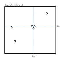
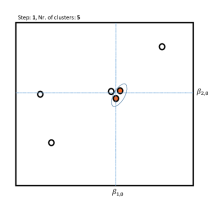
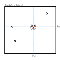
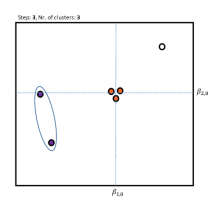
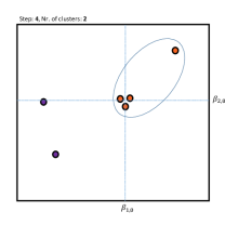
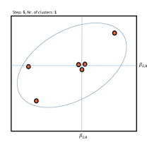
Figure 2: Illustration of the Algorithm with Two Regressors

Appendix B Properties of just-identified estimates when $P\geq 1$

There are $\binom{J}{P}$ just-identified models. We write the corresponding just-identified estimators for $\bm{\beta}$ and $\bm{\alpha}$ analogously to the proof of Proposition A.5 in [31] for the case $P=1$. First, for an arbitrary $[j]$, partition the matrix $\mathbf{Z}=(\mathbf{Z}_{1}\quad\mathbf{Z}_{2})$, where $\mathbf{Z}_{1}$ is a $n\times P$ matrix containing the $[j]$-th columns of $\mathbf{Z}$, and $\mathbf{Z}_{2}$ is a $n\times(J-P)$ matrix containing the remaining columns of $\mathbf{Z}$. $\bm{\gamma}=(\bm{\gamma}_{1}^{\prime}\quad\bm{\gamma}_{2}^{\prime})^{\prime}$ is the equivalent partition of the matrix of first-stage coefficients. $\mathbf{Z^{*}}=[\hat{\mathbf{D}}\quad\mathbf{Z}_{2}]$, then $\mathbf{Z^{*}}=\mathbf{Z}\hat{\mathbf{H}}$, with

$$\bm{\hat{H}}=\left({\begin{array}[]{cc}\hat{\bm{\gamma}}_{1}&0\\ \hat{\bm{\gamma}}_{2}&\mathbf{I}_{J-P}\\ \end{array}}\right);\quad\bm{\hat{H}^{-1}}=\left({\begin{array}[]{cc}\hat{\bm{\gamma}}_{1}^{-1}&0\\ -\hat{\bm{\gamma}}_{2}\hat{\bm{\gamma}}_{1}^{-1}&\mathbf{I}_{J-P}\\ \end{array}}\right)$$

The just-identified 2SLS estimators using $\mathbf{Z}_{[j]}$ as instruments and controlling for the remaining instruments can be written as

$$(\hat{\bm{\beta}}_{[j]}\quad\hat{\bm{\alpha}}_{[j]}^{\prime})^{\prime}=\hat{\mathbf{H}}^{-1}\hat{\bm{\Gamma}}=\hat{\mathbf{H}}^{-1}(\mathbf{Z}^{\prime}\mathbf{Z})^{-1}\mathbf{Z}^{\prime}(\mathbf{D}\bm{\beta}+\mathbf{Z}\bm{\alpha}+\mathbf{u})=\hat{\mathbf{H}}^{-1}(\hat{\bm{\gamma}}\bm{\beta}+\bm{\alpha}+(\mathbf{Z}^{\prime}\mathbf{Z})^{-1}\mathbf{Z}^{\prime}\mathbf{u})$$

Note that $\hat{\bm{\gamma}}\bm{\beta}+\bm{\alpha}$ is equal to

$$\left(\begin{array}[]{c}\hat{\bm{\gamma}}_{1}\bm{\beta}+\bm{\alpha}_{1}\\ \hat{\bm{\gamma}}_{2}\bm{\beta}+\bm{\alpha}_{2}\\ \end{array}\right)\text{.}$$

By Assumption 4, we have the following asymptotics

$$plim(\hat{\bm{\beta}}_{[j]}^{\prime}\quad\hat{\bm{\alpha}}_{[j]}^{\prime})^{\prime}=plim(\mathbf{\hat{H}^{-1}}\left(\begin{array}[]{c}\hat{\bm{\gamma}}_{1}\bm{\beta}+\bm{\alpha}_{1}\\ \hat{\bm{\gamma}}_{2}\bm{\beta}+\bm{\alpha}_{2}\end{array}\right))=\left(\begin{array}[]{c}\bm{\beta}+\bm{\gamma}_{1}^{-1}\bm{\alpha}_{1}\\ -\bm{\gamma}_{2}\bm{\gamma}_{1}^{-1}\bm{\alpha}_{1}+\bm{\alpha}_{2}\end{array}\right)$$

We denote the $\binom{J}{P}$ $P\times 1$-dimensional inconsistency terms as $plim(\hat{\bm{\beta}}_{[j]}-\bm{\beta})=\bm{\gamma}_{[j]}^{-1}\bm{\alpha}_{[j]}=\mathbf{q}$.

Appendix C $\mathcal{F}_{0}$ consists of valid IVs only

Next, we show that the family with $\mathbf{q}=\mathbf{0}$ is composed of valid IVs with $\bm{\alpha}_{1}=\mathbf{0}$, only. Let $\bm{\gamma}$, $\mathbf{Z}$ and $\bm{\alpha}$ be partitioned the same way as in Appendix B.

Remark 1.

$\bm{\alpha}_{1}=\mathbf{0}$ is necessary and sufficient for $\mathbf{q}=\mathbf{0}$.

Proof:

First prove sufficiency: Direct proof: Assume $\bm{\alpha}_{1}=\mathbf{0}$ holds. $\mathbf{q}=\bm{\gamma}_{1}^{-1}\bm{\alpha}_{1}=\mathbf{0}$ follows directly.
Second, prove necessity: Proof by contraposition: Assume $\bm{\alpha}_{1}\neq\mathbf{0}$, then $\bm{\gamma}_{1}^{-1}\bm{\alpha}_{1}\neq\mathbf{0}$. The latter inequality holds, because otherwise the columns of $\bm{\gamma}_{1}^{-1}$ are linearly dependent, and $\bm{\gamma}_{1}^{-1}$ is not invertible and hence $(\bm{\gamma}_{1}^{-1})^{-1}=\bm{\gamma}_{1}$ does not exist, which it clearly does, by Assumption 1.a. ∎

This also implies that $\mathcal{F}_{0}$ consists of valid IVs only and all combinations $[j]:\bm{\gamma}_{1}^{-1}\bm{\alpha}_{1}=\mathbf{0}$ are elements of $\mathcal{F}_{0}$. Hence, the following remark directly follows:

Remark 2.

$|\mathcal{F}_{0}|=\binom{g}{P}$.

Appendix D Oracle Properties

This section gives proofs for Lemma 1 and Theorems 1 and 3. All proofs apply for the general case that $P\geq 1$.

D.1 Proof of Lemma 1

Overall, we want to show that the probability that a cluster $\mathcal{S}_{j}$ with elements from the true underlying partition $\mathcal{S}_{0q}$ is merged with a cluster with elements from the same partition $\mathcal{S}_{0q}$ goes to 1.

The proof is structured as follows:

1. We note that the means of clusters which are associated with elements from the same family also converge to the same vector as each estimator in the cluster.
   

2. Merging two clusters which are associated only with elements from the same family is equivalent to the two clusters having minimal distance.
   

3. We show that clusters which are associated with members from the same family have distance zero and clusters which are associated with elements from different families have non-zero distance, with probability going to one.

Proof.

Part 1: Consider

$$\begin{split}[j],[k]\in\mathcal{F}_{q}\,,\quad\mathbf{q}\in\mathbb{R}^{P}\\ [l]\in\mathcal{F}_{r}\,,\quad\mathbf{r}\in\mathbb{R}^{P},\quad\mathbf{r}\neq\mathbf{q}\\ \end{split}$$

Under Assumptions 1 - 5:

$$\begin{split}plim(\hat{\bm{\beta}}_{[j]})=plim(\hat{\bm{\beta}}_{[k]})=\mathbf{q}\\ plim(\hat{\bm{\beta}}_{[l]})=\mathbf{r}\end{split}$$ (11)

Let $\mathcal{S}_{j}$ and $\mathcal{S}_{k}$ be clusters associated with elements from the same family: $\mathcal{S}_{j}$, $\mathcal{S}_{k}\subset\mathcal{S}_{0q}$ and $\mathcal{S}_{l}\subset\mathcal{S}_{0r}$.

$$plim\,\,\bar{\mathcal{S}}_{j}=\frac{\sum\limits_{\hat{\beta}_{[j]}\in\mathcal{S}_{j}}\bm{\hat{\beta}_{[j]}}}{|\mathcal{S}_{j}|}=\frac{|\mathcal{S}_{j}|\mathbf{q}}{|\mathcal{S}_{j}|}\text{ where }\mathcal{S}_{j}\subset\mathcal{S}_{0q}$$ (12)

and hence

$$plim(\bar{\mathcal{S}}_{j})=\mathbf{q}\text{.}$$

Part 2: Consider the case where the Algorithm decides whether to merge two clusters, $\mathcal{S}_{j}$ and $\mathcal{S}_{k}$, containing estimators using combinations from the same family, or to merge two clusters from different underlying partitions, $\mathcal{S}_{j}$ and $\mathcal{S}_{l}$. The two clusters which are closest in terms of their weighted Euclidean distance are merged first. Hence, we need to consider the distances between $\mathcal{S}_{j}$ and $\mathcal{S}_{k}$, $\mathcal{S}_{j}$ and $\mathcal{S}_{l}$, as well as $\mathcal{S}_{k}$ and $\mathcal{S}_{l}$.

$\mathcal{S}_{j}$ is merged with a cluster with elements of its own $\mathcal{S}_{0q}$ iff $\frac{|\mathcal{S}_{j}||\mathcal{S}_{k}|}{|\mathcal{S}_{j}|+|\mathcal{S}_{k}|}||\bar{\mathcal{S}}_{j}-\bar{\mathcal{S}}_{k}||^{2}<\frac{|\mathcal{S}_{j}||\mathcal{S}_{l}|}{|\mathcal{S}_{j}|+|\mathcal{S}_{l}|}||\bar{\mathcal{S}}_{j}-\bar{\mathcal{S}}_{l}||^{2}$. The following two are hence equivalent

$$lim\,P(\mathcal{S}_{j}\cup\mathcal{S}_{k}=\mathcal{S}_{jk}\subseteq\mathcal{S}_{0q})=1$$

$$\Leftrightarrow\quad lim\,P(\frac{|\mathcal{S}_{j}||\mathcal{S}_{k}|}{|\mathcal{S}_{j}|+|\mathcal{S}_{k}|}||\bar{\mathcal{S}}_{j}-\bar{\mathcal{S}}_{k}||^{2}<\frac{|\mathcal{S}_{j}||\mathcal{S}_{l}|}{|\mathcal{S}_{j}|+|\mathcal{S}_{l}|}||\bar{\mathcal{S}}_{j}-\bar{\mathcal{S}}_{l}||^{2})=1$$ (13)

where $\mathcal{S}_{jk}$ is the new merged cluster.

Part 3: We want to prove equation (13) in the following. We can then prove $lim\,P(\frac{|\mathcal{S}_{j}||\mathcal{S}_{k}|}{|\mathcal{S}_{j}|+|\mathcal{S}_{k}|}||\bar{\mathcal{S}}_{k}-\bar{\mathcal{S}}_{j}||^{2}<\frac{|\mathcal{S}_{k}||\mathcal{S}_{l}|}{|\mathcal{S}_{k}|+|\mathcal{S}_{l}|}||\bar{\mathcal{S}}_{k}-\bar{\mathcal{S}}_{l}||^{2})=1$ by changing the subscripts.

First, define $a=\frac{|\mathcal{S}_{j}||\mathcal{S}_{k}|}{|\mathcal{S}_{j}|+|\mathcal{S}_{k}|}||\bar{\mathcal{S}}_{j}-\bar{\mathcal{S}}_{k}||^{2}$ , $b=\frac{|\mathcal{S}_{j}||\mathcal{S}_{l}|}{|\mathcal{S}_{j}|+|\mathcal{S}_{l}|}||\bar{\mathcal{S}}_{j}-\bar{\mathcal{S}}_{l}||^{2}$ and $c=\frac{|\mathcal{S}_{j}||\mathcal{S}_{l}|}{|\mathcal{S}_{j}|+|\mathcal{S}_{l}|}(\mathbf{q}-\mathbf{r})^{\prime}(\mathbf{q}-\mathbf{r})$.

Under (12)

$$\begin{split}plim(a)&=\bm{0}\\ plim(b)&=c\\ \end{split}$$

To show: $\underset{n\rightarrow\infty}{\lim}\,P(a<b)=1$.

Proof by contradiction: Show that $\underset{n\rightarrow\infty}{\lim}\,P(b<a)\neq 0$ leads to a contradiction. Let $\lim$ imply $\underset{n\rightarrow\infty}{\lim}$ in the following. By the definitions of convergence in probability, it follows that

$$\lim\,P(a<\varepsilon)=1$$ (14)

and

$$\lim\,P(|b-c|<\varepsilon)=1\text{.}$$ (15)

for any $\varepsilon$. Therefore, $\lim\,P(a<b)\neq 0$ and $\lim\,P(a<\varepsilon)=1$ imply $\lim\,P(b<\varepsilon)\neq 0$.

Now, consider $\varepsilon<\frac{1}{2}c$.

Then,

$$\lim\,P(b<\frac{1}{2}c)\neq 0$$ (16)

Because of the absolute value $b-c$, consider two cases, $b<c$ and $b>c$. If $b<c$: $\lim\,P(c-b<\frac{1}{2}c)=1\,\Leftrightarrow\,\lim\,P(c-b>\frac{1}{2}c)=0$. $\Rightarrow\,\lim\,P(b<\frac{1}{2}c)=0$, a contradiction with (16). If $b\geq c$: $a<\varepsilon<\frac{1}{2}c<c\leq b$ and hence $\lim\,P(a<b)=1\,\Leftrightarrow\,\lim\,P(b\leq a)=0$, again a contradiction. ∎

∎

D.2 Proof of Theorem 1

Proof.

The proof for Theorem 1 is structured as follows:

1. We show that asymptotically the selection path generated by Algorithm 1 contains $\mathcal{F}_{0}$, the family formed by all the valid instrumental variables.

2. We show that Algorithm 2 can recover $\mathcal{F}_{0}$ from the selection path from Algorithm 1.

Part 1 follows from Corollary 2 directly.

Part 2: Firstly, we establish the properties of the Sargan statistic. The following two equations can be also found in WLHB (p.10). Let $\mathcal{I}$ be the true set of invalid instruments and $\mathcal{V}$ be the true set of valid instruments. The oracle model is

$$\mathbf{y}=\mathbf{D}\bm{\beta}+\mathbf{Z}_{\mathcal{I}}\bm{\alpha}_{\mathcal{I}}+\mathbf{u}=\mathbf{X}_{\mathcal{I}}\bm{\theta}_{\mathcal{I}}+\mathbf{u}$$

with $\mathbf{X}_{\mathcal{I}}=\left[\mathbf{D}\quad\mathbf{Z}_{\mathcal{I}}\right]$ and $\bm{\theta}_{\mathcal{I}}=\left[\bm{\beta}\quad\bm{\alpha}_{\mathcal{I}}^{\prime}\right]^{\prime}$, the Sargan test statistic is given by

$$S(\hat{\bm{\theta}}_{\mathcal{I}})=\frac{\hat{\mathbf{u}}(\hat{\bm{\theta}}_{\mathcal{I}})^{\prime}\mathbf{Z}_{\mathcal{I}}(\mathbf{Z}_{\mathcal{I}}^{\prime}\mathbf{Z}_{\mathcal{I}})^{-1}\mathbf{Z}_{\mathcal{I}}^{\prime}\hat{\mathbf{u}}(\hat{\bm{\theta}}_{\mathcal{I}})}{\hat{\mathbf{u}}(\hat{\theta}_{\mathcal{I}})^{\prime}\hat{\mathbf{u}}(\hat{\bm{\theta}}_{\mathcal{I}})/n}$$ (17)

where $\hat{\mathbf{u}}(\hat{\bm{\theta}})=\mathbf{y}-\mathbf{X}_{\mathcal{I}}\hat{\bm{\theta}}_{\mathcal{I}}$, with $\hat{\bm{\theta}}_{\mathcal{I}}$ the 2SLS estimator of $\bm{\theta}_{\mathcal{I}}$.

Let $\hat{\mathcal{I}}$ be the estimated set of invalid instruments and $\hat{\mathcal{V}}$ be the estimated set of valid instruments where $\hat{\mathcal{I}}=\mathcal{J}\setminus\hat{\mathcal{V}}$. Following Proposition $3.2$ in [29], the Sargan statistic has the following properties:

Property 3.

Properties of the Sargan statistic

1. For all the $|\mathcal{\hat{\mathcal{V}}}|\choose P$ combinations of the instruments from $\hat{\mathcal{V}}$, if the IVs contained in them belong to the same family, then: $S(\hat{\bm{\theta}}_{\mathcal{\hat{\mathcal{I}}}})\overset{d}{\rightarrow}\chi^{2}_{|\mathcal{J}|-|\mathcal{\hat{\mathcal{I}}}|-P}$

2. For all the $|\mathcal{\hat{\mathcal{V}}}|\choose P$ combinations of the instruments from $\hat{\mathcal{V}}$, if the IVs contained in them belong to a mixture of families, then: $S(\hat{\bm{\theta}}_{\mathcal{\hat{\mathcal{I}}}})=O_{p}(n)$.

With these properties we can show that the downward testing procedure described in Algorithm 2 selects valid instruments consistently with $\xi_{n,J-|\hat{\mathcal{I}}|-P}\rightarrow\infty\text{ for }n\rightarrow\infty\text{, and }\xi_{n,J-|\hat{\mathcal{I}}|-P}=o(n)\text{.}$ Let the number of clusters formed in Algorithm 1 at some certain step be $K$, e.g. at Step 1, $K={J\choose P}$ and at Step 2, $K={J\choose P}-1$ etc. Let the true number of families be $Q$. Consider applying the Sargan test to the model selected by the largest cluster at the each step under the following scenarios:

1. $1\leq K<Q$. For each of these steps, the largest cluster is either associated with a mixture of different families, or with one family.

   • Consider the case where the largest cluster is associated with a mixture of different families. Then by Property 3 and $\xi_{n,J-|\hat{\mathcal{I}}|-P}=o(n)$, we have

     $$\underset{n\rightarrow\infty}{lim}P(S(\hat{\bm{\theta}}_{\hat{\mathcal{I}}})<\xi_{n,J-|\hat{\mathcal{I}}|-P})=0\text{.}$$

     In this case, asymptotically the Sargan test would be rejected and the downward testing procedure moves to the next step.

   • Consider the case where the largest cluster is associated with one family. Then this family must be $\mathcal{F}_{0}$ as by Assumption 6.a, $\mathcal{F}_{0}$ is the largest family among all $Q$ families. Then following Property 3 and $\xi_{n,J-|\hat{\mathcal{I}}|-P}\rightarrow\infty$ for the Sargan test we have

     $$\underset{n\rightarrow\infty}{lim}P(S(\hat{\bm{\theta}}_{\hat{\mathcal{I}}})<\xi_{n,J-|\hat{\mathcal{I}}|-P})=1\text{.}$$ (18)

     indicating that $\mathcal{V}$ would be selected as the set of valid instruments asymptotically.

2. $K=Q$. By Corollary 2 we know that the $K$ clusters are associated with the $Q$ families respectively, and by Assumption 6.a, the cluster associated with $\mathcal{F}_{0}$ is the largest cluster. Then applying the Sargan test at this step would be testing all the valid instruments, hence we also have Equation (18) and Algorithm 2 selects $\mathcal{V}$ as the set of valid instruments.

To summarize, asymptotically, at steps $1\leq K<Q$, Algorithm 2 only stops when $\mathcal{F}_{0}$ forms the largest cluster and hence selects the oracle model, otherwise it moves to step $K=Q$ and selects the oracle model. Combine Part 1 and Part 2, we prove Theorem 1.

∎

D.3 Proof of Theorem 3

The proof of Theorem 3 works in the same way as the proof of Theorem 1.

Proof.

The proof for Theorem 3 is structured as follows:

1. We note that asymptotically the selection path generated from Algorithm 1 contains all groups $\mathcal{G}_{q}$.

2. We show that Algorithm 2 can recover all $\mathcal{G}_{q}$ from the selection path from Algorithm 1.

Part 1 again follows directly from Corollary 2.

Part 2: Firstly, we establish the properties of the Sargan statistic.

Property 4.

Properties of the Sargan statistic

1. For all combinations of instruments from $\hat{\mathcal{G}}_{k}$, if their just-identified estimators are associated with the same group, then: $S(\hat{\bm{\theta}}_{\mathcal{\hat{\mathcal{G}}}_{k}})\overset{d}{\rightarrow}\chi^{2}_{J-|\mathcal{\hat{\mathcal{G}}}_{k}|-P}$

2. For all combinations of instruments from $\hat{\mathcal{G}}_{k}$, if their just-identified estimators are associated with a mixture of groups, then: $S(\hat{\bm{\theta}}_{\mathcal{\hat{\mathcal{G}}}_{k}})=O_{p}(n)$.

As before, $\xi_{n,J-|\hat{\mathcal{I}}|-P}\rightarrow\infty\text{ for }n\rightarrow\infty\text{, and }\xi_{n,J-|\hat{\mathcal{I}}|-P}=o(n)\text{.}$ Consider applying the Sargan test to each cluster separately at the following steps under the following scenarios:

1. $1\leq K<Q$, i.e. the number of clusters is smaller than the number of groups. For each of these steps, at least one cluster is associated with a mixture of different groups.

   When one cluster is created by a mixture of different groups, by Property 4, we have

   $$\underset{n\rightarrow\infty}{lim}P(S(\hat{\bm{\theta}}_{\mathcal{G}_{q}})<\xi_{n,J-|\mathcal{G}_{q}|-P})=0\text{.}$$ (19)

   In this case, asymptotically at least one of the the Sargan tests would be rejected and the downward testing procedure moves to the next step.

2. $K=Q$. By Corollary 2 we know that the $K$ clusters are formed by the $Q$ groups respectively and $\hat{\mathcal{G}}_{k}=\mathcal{G}_{q}$ for all $q$. Then for each of the $K$ tests we have

   $$S(\hat{\bm{\theta}}_{\mathcal{\hat{\mathcal{G}}}_{k}})=S(\hat{\bm{\theta}}_{\mathcal{G}_{q}})\text{.}$$ (20)

   By Property 4 and $\xi_{n,J-|\mathcal{G}_{q}|-P}=o(n)$, we have

   $$\underset{n\rightarrow\infty}{lim}P(S(\hat{\bm{\theta}}_{\mathcal{G}_{q}})<\xi_{n,J-|\hat{\mathcal{I}}|-P})=1\text{.}$$

   In this case, Algorithm 2 stops.

   Then applying the Sargan tests to each group at this step will be testing IVs from the same group each time, hence we also have Equation (19).

To summarize, asymptotically, at steps $1\leq K<Q$, Algorithm 2 does not stop; then it moves to step $K=Q$ and selects the oracle model.

Combine Part 1 and Part 2, we prove Theorem 1. ∎

References

- [1] Charu C Aggarwal, Alexander Hinneburg and Daniel A Keim “On the Surprising Behavior of Distance Metrics in High Dimensional Space” In International Conference on Database Theory, 2001, pp. 420–434 Springer
- [2] Joseph G Altonji and David Card “The Effects of Immigration on the Labor Market Outcomes of Less-Skilled Natives” In Immigration, Trade, and the Labor Market University of Chicago Press, 1991, pp. 201–234
- [3] Renato Cordeiro Amorim, Vladimir Makarenkov and Boris Mirkin “A-Wardp: Effective hierarchical clustering using the Minkowski metric and a fast k-means initialisation” In Information Sciences 370 Elsevier, 2016, pp. 343–354
- [4] Donald WK Andrews “Consistent Moment Selection Procedures for Generalized Method of Moments Estimation” In Econometrica 67.3 Wiley Online Library, 1999, pp. 543–563
- [5] Joshua D Angrist and Alan B Krueger “Does Compulsory School Attendance Affect Schooling and Earnings?” In The Quarterly Journal of Economics 106.4 MIT Press, 1991, pp. 979–1014
- [6] Nicolas Apfel “Relaxing the Exclusion Restriction in Shift-Share Instrumental Variable Estimation” In Available at SSRN 3408682, 2021
- [7] Gaetano Basso and Giovanni Peri “The Association Between Immigration and Labor Market Outcomes in the United States” In IZA Discussion Paper 9436 IZA Discussion Paper, 2015
- [8] Alexandre Belloni, Daniel Chen, Victor Chernozhukov and Christian Hansen “Sparse Models and Methods for Optimal Instruments with an Application to Eminent Domain” In Econometrica 80.6 Wiley Online Library, 2012, pp. 2369–2429
- [9] John Bound, David A Jaeger and Regina M Baker “Problems With Instrumental Variables Estimation When the Correlation Between the Instruments and the Endogenous Explanatory Variable Is Weak” In Journal of the American Statistical Association 90.430 Taylor & Francis, 1995, pp. 443–450
- [10] Mehmet Caner “Near Exogeneity and Weak Identification in Generalized Empirical Likelihood Estimators: Many Moment Asymptotics” In Journal of Econometrics 182.2 Elsevier, 2014, pp. 247–268
- [11] Timothy G Conley, Christian B Hansen and Peter E Rossi “Plausibly Exogenous” In Review of Economics and Statistics 94.1 MIT Press, 2012, pp. 260–272
- [12] Tatyana Deryugina, Garth Heutel, Nolan H Miller, David Molitor and Julian Reif “The Mortality and Medical Costs of Air Pollution: Evidence from Changes in Wind Direction” In American Economic Review 109.12, 2019, pp. 4178–4219
- [13] Christian Dustmann, Uta Schönberg and Jan Stuhler “The Impact of Immigration: Why Do Studies Reach Such Different Results?” In Journal of Economic Perspectives 30.4, 2016, pp. 31–56
- [14] Alexandre Godzinski and Milena Suarez Castillo “Disentangling the Effects of Air Pollutants With Many Instruments” In Journal of Environmental Economics and Management 109 Elsevier, 2021, pp. 102489
- [15] Paul Goldsmith-Pinkham, Isaac Sorkin and Henry Swift “Bartik Instruments: What, When, Why, and How” In American Economic Review, 2020
- [16] Zijian Guo “Post-selection Problems for Causal Inference with Invalid Instruments: A Solution Using Searching and Sampling” In arXiv preprint arXiv:2104.06911, 2021
- [17] Zijian Guo, Hyunseung Kang, T Tony Cai and Dylan S Small “Confidence Intervals for Causal Effects with Invalid Instruments by Using Two-Stage Hard Thresholding with Voting” In Journal of the Royal Statistical Society: Series B (Statistical Methodology) Wiley Online Library, 2018
- [18] Lars Peter Hansen “Large Sample Properties of Generalized Method of Moments Estimators” In Econometrica: Journal of the Econometric Society JSTOR, 1982, pp. 1029–1054
- [19] Guido W Imbens and Joshua D Angrist “Estimation and Identification of Local Average Treatment Effects” In Econometrica 62, 1994, pp. 467–475
- [20] David A Jaeger, Joakim Ruist and Jan Stuhler “Shift-Share Instruments and the Impact of Immigration”, 2020
- [21] Hyunseung Kang, Youjin Lee, T Tony Cai and Dylan S Small “Two Robust Tools for Inference About Causal Effects With Invalid Instruments” In Biometrics 78.1 Wiley Online Library, 2022, pp. 24–34
- [22] Hyunseung Kang, Anru Zhang, Tianwen T Cai and Dylan S Small “Instrumental Variables Estimation with Some Invalid Instruments and Its Application to Mendelian Randomization” In Journal of the American Statistical Association 111.513 Taylor & Francis, 2016, pp. 132–144
- [23] Matthew A Masten and Alexandre Poirier “Salvaging falsified instrumental variable models” In Econometrica 89.3 Wiley Online Library, 2021, pp. 1449–1469
- [24] Steven Ruggles, Katie Genadek, Ronald Goeken, Josiah Grover and Matthew Sobek “Integrated Public Use Microdata Series: Version 6.0 [Dataset]” In Minneapolis: University of Minnesota 23, 2015, pp. 56
- [25] Doug Staiger and James Stock “Instrumental Variables Regression with Weak Instruments” In Econometrica 65.3 Econometric Society, 1997, pp. 557–586
- [26] Joe H Jr Ward “Hierarchical Grouping to Optimize an Objective Function” In Journal of the American Statistical Association 58.301 Taylor & Francis Group, 1963, pp. 236–244
- [27] Frances Wensley, Pei Gao, Stephen Burgess, Stephen Kaptoge, Emanuele Di Angelantonio, Tina Shah, James C Engert, Robert Clarke, George Davey-Smith and Børge G Nordestgaard “Association Between C Reactive Protein and Coronary Heart Disease: Mendelian Randomisation Analysis Based on Individual Participant Data” In BMJ 342.feb15, 2011, pp. d548
- [28] Frank Windmeijer “Two-Stage Least Squares as Minimum Distance” In The Econometrics Journal 22.1 Oxford University Press, 2019, pp. 1–9
- [29] Frank Windmeijer “Two-stage least squares as minimum distance” In The Econometrics Journal 22.1 Oxford University Press, 2019, pp. 1–9
- [30] Frank Windmeijer, Helmut Farbmacher, Neil Davies and George D Smith “On the Use of the Lasso for Instrumental Variables Estimation with Some Invalid Instruments” In Journal of the American Statistical Association 114.527 Taylor & Francis, 2019, pp. 1339–1350
- [31] Frank Windmeijer, Xiaoran Liang, Fernando Hartwig and Jack Bowden “The Confidence Interval Method for Selecting Valid Instrumental Variables” In Journal of the Royal Statistical Society: Series B Forthcoming Wiley, 2021
- [32] Jeffrey M Wooldridge “Econometric analysis of cross section and panel data” MIT press, 2010