Temporal Logic Task Allocation in Heterogeneous Multi-Robot Systems

Abstract

In this paper, we consider the problem of optimally allocating tasks, expressed as global Linear Temporal Logic (LTL) specifications, to teams of heterogeneous mobile robots. The robots are classified in different types that capture their different capabilities, and each task may require robots of multiple types. The specific robots assigned to each task are immaterial, as long as they are of the desired type. Given a discrete workspace, our goal is to design paths, i.e., sequences of discrete states, for the robots so that the LTL specification is satisfied. To obtain a scalable solution to this complex temporal logic task allocation problem, we propose a hierarchical approach that first allocates specific robots to tasks using the information about the tasks contained in the Nondeterministic B$\ddot{\text{u}}$chi Automaton (NBA) that captures the LTL specification, and then designs low-level executable plans for the robots that respect the high-level assignment. Specifically, we first prune and relax the NBA by removing all negative atomic propositions. This step is motivated by “lazy collision checking” methods in robotics and allows to simplify the planning problem by checking constraint satisfaction only when needed. Then, we extract sequences of subtasks from the relaxed NBA along with their temporal orders, and formulate a Mixed Integer Linear Program (MILP) to allocate these subtasks to the robots. Finally, we define generalized multi-robot path planning problems to obtain low-level executable robot plans that satisfy both the high-level task allocation and the temporal constraints captured by the negative atomic propositions in the original NBA. We show that our method is complete for a subclass of LTL that covers a broad range of tasks and present numerical simulations demonstrating that it can generate paths with lower cost, considerably faster than existing methods.

I Introduction

Robot motion planning traditionally consists of generating robot trajectories between a start and a goal region, while avoiding obstacles [lavalle2006planning]. More recently, new planning methods have been proposed that can handle a richer class of tasks than standard point-to-point navigation that also include temporal goals subject to time constraints. Such tasks can be captured using formal languages, such as Linear Temporal Logic (LTL) [baier2008principles], and include sequencing or coverage [fainekos2005temporal], data gathering [guo2017distributed], intermittent communication [kantaros2018distributed], and persistent surveillance [leahy2016persistent], to name a few. A survey on formal specifications and synthesis techniques for robotic systems can be found in [luckcuck2019formal].

In this paper, we consider LTL tasks that require robots of different types to collaborate to satisfy the specification. The different robot types capture the different robot capabilities, and each task may require robots of multiple types to accomplish. The specific robots assigned to each task are immaterial, as long as they are of the desired type. An example of such an LTL task is: At most five robots of type 1 pick up the mail by visiting houses in a given order. Next, visit a delivery site. Never leave the delivery site until one ground robot of type 2 is present to pick up the mail (a robot of type 2 can carry mail from at most 5 robots of type 1). Repeat this process infinitely often. In this task, several robots are required to work cooperatively and meet simultaneously at the same place. Note that the specific robots to participate in this task are not important and are not specified by the LTL formula. Instead, it is only required that no more than five robots of type 1 and exactly one robot of type 2 collaborate to accomplish this task. Therefore, there are multiple ways that this LTL task can be satisfied, which grow combinatorially with the number of robots, robot types, and the complexity of the LTL task. We refer to this problem as the Multi-Robot Task Allocation (MRTA) problem for LTL tasks, in short, LTL-MRTA. Existing control synthesis methods under temporal logic specifications, such as the ones proposed in [smith2010optimal, ulusoy2013optimality, guo2015multi, kantaros15asilomar], build a large product automaton composed of the Nondeterministic B$\ddot{\text{u}}$chi Automaton (NBA) that captures the LTL specification and the discrete transition systems describing the motion of each one of the robots in the world. Then, these methods employ graph search techniques on this product graph to find the optimal plan that satisfies the LTL specification. However, as the number of robots, the size of the environment, and the complexity of the LTL task grows, the size of this product graph grows exponentially large and, therefore, graph search methods become intractable. This is more so the case for LTL-MRTA problems as the number of possible assignments of robots to tasks increases the complexity of the LTL specification dramatically.

To mitigate the computational complexity of the LTL-MRTA problem, we propose a novel hierarchical approach that first allocates specific robots to tasks using the information about tasks provided by the Nondeterministic B$\ddot{\text{u}}$chi Automaton (NBA) that captures the LTL specification, and then designs low-level executable plans for the robots that respect the high-level assignment. Specifically, we first prune and relax the NBA by removing all negative atomic propositions. This step is motivated by ”lazy collision checking” methods in robotics [sanchez2003single, hauser2015lazy] and allows to simplify the planning problem by checking constraint satisfaction only when needed. Then, we extract sequences of subtasks from the relaxed NBA along with their temporal orders, and formulate a Mixed Integer Linear Program (MILP), inspired by the vehicle routing problem [bredstrom2008combined], to allocate these subtasks to the robots, while respecting the temporal order between subtasks. The solution to this MILP generates a time-stamped task allocation plan for each robot, which is a sequence of essential waypoints that the robot needs to visit. Finally, given this time-stamped task allocation plan for each robot, we formulate a sequence of generalized multi-robot path planning (GMRPP) problems, one for each subtask, to obtain executable paths that also respect the negative atomic propositions that were relaxed from the original NBA. We show through extensive simulations that our method can handle LTL-MRTA problems with up to $10^{90}$ states in the product graph, considerably outperforming existing methods. Moreover, we provide theoretical guarantees on the completeness and soundness of our proposed framework, under mild assumptions on the structure of the NBA that were satisfied by all meaningful LTL specifications we considered in practice, no matter their complexity. While not theoretically optimal, our method is still able to improve on the cost of the returned plans, unlike existing methods in the literature that only focus on feasibility.

I-A Related work

In existing literature on optimal control synthesis methods from LTL specifications, LTL tasks are either assigned locally to the robots in a multi-robot team, as in [guo2015multi, tumova2016multi] or a global LTL specification is assigned to the team that captures the collective behavior of all robots. In the latter case, the global LTL specification can explicitly assign tasks to the individual robots, as in [loizou2004automatic, smith2011optimal, saha2014automated, kantaros2015intermittent, kantaros2017sampling, kantaros2018distributedOpt, kantaros2018sampling, kantaros2018temporal, kantaros2020stylus, xluo_CDC19, luo2019abstraction], or it may not explicitly assign tasks to the robots as in [kloetzer2011multi, shoukry2017linear, moarref2017decentralized, lacerda2019petri], and our current work in this paper.

Global temporal logic specifications that do not explicitly allocate tasks to robots typically need to be decomposed in order to obtain the required allocation. For example, [tumova2015decomposition, kantaros2016distributed] decompose a global specification directly into local specifications and assign them to individual robots. Similarly, [camacho2017non, xluo_CDC19, camacho2019ltl, schillinger2019hierarchical] decompose a global specification into multiple subtasks by exploiting the structure of the finite automata. Particularly, [camacho2017non] convert temporal planning problems to standard planning problems by defining actions based on transitions in the NBA, while [xluo_CDC19] define subtasks associated with transitions in the NBA and synthesize plans for these subtasks which they store in a library so that they can be reused to efficiently synthesize plans for new LTL formulas. [schillinger2019hierarchical] also define subtasks associated with transitions in the automaton, but use reinforcement learning to learn plans that execute these subtasks under uncertainty. [camacho2019ltl] also use reinforcement learning but with the purpose of converting formal languages to reward machines that capture the structure of the task. Similar to these works, here too we define subtasks associated with transitions in the NBA. However, we do not assume that these subtasks are preassigned to the robots.

Temporal logic control synthesis without an explicit assignment of robots to tasks has been considered in [karaman2011linear] that combine the vehicle routing problem with metric temporal logic specifications and leverage MILP to solve this problem for heterogeneous robots. However, this approach can only handle finite horizon tasks and does not design the low-level executable paths as we do here. An alternative approach is proposed in [chen2011formal, leahy2015distributed] that decomposes a global automaton into individual automata that are assigned to the heterogeneous robots and then builds a synchronous product of these automata to synthesize parallel plans. However, the size of the synchronous product automaton grows exponentially large with the number of robots. Also, the requirement that parallel plans exist does not allow application of this method to tasks that lack such parallel executions. Furthermore, this method also focuses only on finite robot trajectories. In relevant literature, teams of homogeneous robots have also been modeled using Petri Nets as in [lacerda2019petri, kloetzer2020path]. Specifically, [lacerda2019petri] propose a job shop problem under safe temporal logic specifications, but do not consider the “eventually” operator so that liveness in terms of good future outcomes can not be guaranteed. Additionally, this approach only focuses on robot coordination at the task level without considering execution. To the contrary, [kloetzer2020path] select multiple shortest accepting runs in the NBA and for each accepting run, determine whether an executable plan exists. Finally, [schillinger2018decomposition, schillinger2018simultaneous, faruq2018simultaneous, banks2020multi] automatically decompose the automaton representation of the LTL formula into independent subtasks that can be fulfilled by different robots. However, they only consider LTL formulas that can be satisfied by finite robot trajectories, limiting the applicability of the proposed method to tasks such as recurrent sequencing and persistent monitoring. Also, subtasks subject to precedence relations can only be executed by a single robot.

Common in the above approaches is that they do not consider cooperative tasks where robots of the same or different types need to meet at a common location to complete a task, Such tasks require strong synchronization between robots. In our recent work [kantaros2018sampling, kantaros2020stylus], we have proposed a sampling-based planning method named STyLuS${}^{*}$ that incrementally builds trees to approximate the product of the NBA and the model of the team. Using the powerful biased sampling method proposed in [kantaros2020stylus], STyLuS${}^{*}$ can synthesize plans for product automata with up to $10^{800}$ states without considering collision avoidance. However, STyLuS${}^{*}$ requires global LTL specifications that explicitly assign tasks to robots. Although a subset of specifications we consider here can be converted into explicit LTL formulas by enumerating all possible task assignments and connecting them with “OR” operators, this would result in exponentially long LTL formulas. Furthermore, the biased sampling strategy in STyLuS${}^{*}$ needs a fixed assignment of robots to tasks and biases search towards finding a plan for this fixed assignment. If the assignment is not given, biased STyLuS${}^{*}$ will need to be run combinatorially many times, one for each possible assignment. With unbiased sampling, [kantaros2018sampling] show that STyLuS${}^{*}$ can only solve problems with product automata that have $10^{10}$ states. Instead, our proposed method can synthesize plans for problems with $10^{90}$ states while considering collision avoidance. On the other hand, model-checkers like NuSMV [cimatti2002nusmv], focus on finding feasible paths and are incapable of optimizing cost. As stated in [kantaros2020stylus], NuSMV can only handle problems with $10^{30}$ states, and can not easily process exponentially long LTL formulas generated by explicitly expressing task assignments.

Among other methods that focus on cooperative tasks, [moarref2017decentralized] focus on specifications capturing behaviors of homogeneous robotic swarms at the swarm and individual levels, but they can only impose universal or existential constraints, that is, all robots or some robots visit a certain region. As a result, these specifications are incapable of imposing restrictions on the number of robots that should be present at one place at the same time. This limitation is addressed in [sahin2017provably, sahin2017synchronous, sahin2019multirobot] that relies on counting linear temporal logic (cLTL+/cLTL) to capture constraints on the number of robots that must be present in different regions. Specifically, the authors formulate an Integer Linear Program (ILP) inspired by Bounded Model Checking techniques [biere2006linear], but can only guarantee feasibility of the resulting paths. Instead our hierarchical method also takes into consideration the quality of the solution at each level. A sequential planning approach is proposed in [JoLeVaSaSeTrBe-ISRR-2019] that augments the LTL specification by introducing time and, unlike our proposed approach, plans low-level plans for the robots, one at a time, while treating the other robots as obstacles. Common in the methods in [sahin2017provably, sahin2017synchronous, sahin2019multirobot, JoLeVaSaSeTrBe-ISRR-2019] is that the size of the workspace has a significant effect on the computation time. To mitigate the complexity due to the size of the workspace, [sahin2019multi] propose a hierarchical framework that abstracts the workspace by aggregating states with the same observations. As we show in Section VII, our proposed method scales better than the method in [sahin2019multi], and provides lower cost solutions with less runtime. Also, unlike our method, the completeness of solutions is not guaranteed in [sahin2019multi].

I-B Contributions

The contributions of this paper can be summarized as follows: We propose a new hierarchical approach to the LTL-MRTA problem that first assigns robots to tasks and then plans robot paths that satisfy the high level assignment. Our approach differs from common methods that rely on the product automaton [smith2010optimal, ulusoy2013optimality, guo2015multi] or on the Bounded Model Checking [biere2006linear] in that it directly operates on the NBA. Under mild assumptions on the NBA that are satisfied by a subclass of LTL formulas that cover a broad class of tasks in practice, we showed that our method is complete and sound. While not theoretically optimal, our method still incorporates optimization steps to improve on the cost of the returned plans. To the best of our knowledge, this is the first LTL-MRTA method that is both complete for a subclass of LTL and includes operations to optimize the synthesized plans. The unique aspect of our approach is a clever pruning and relaxation of the NBA that removes all negative atomic propositions, and is motivated by “lazy collision checking” methods in robotics. This step significantly simplifies the planning problem by allowing to check constraint satisfaction only when needed and, as a result, contributes to significantly increasing scalability of our method. To the best of our knowledge, this is the first time that “lazy collision checking” methods that are common in point-to-point navigation are used for high-level robot planning. Another unique aspect of our method is to infer the temporal order of tasks from the automaton, which can capture the parallel execution of subtasks. Compared to existing methods, our approach returns lower cost plans in significantly less time.

The rest of the paper is organized as follows. In Sections II and III we present preliminaries and define the problem under consideration, respectively. We describe the high-level task assignment component of our method in Sections IV and V. Specifically, in Section IV we prune and relax the NBA, identify subtasks from the NBA and infer temporal orders between them. Then, in Section V we formulate a MILP to obtain the high-level plans. In Section VI, we examine the completeness and soundness of these plans, while in Section VII we present simulation results. Finally, Section LABEL:sec:conclusion concludes the paper. For completeness, the low-level component of our method to obtain executable paths, which is based on existing multi-robot path planning techniques, is presented in Appendix LABEL:sec:solution2mrta.

II Preliminaries

II-A Linear temporal logic

Linear Temporal Logic (LTL) is composed of a set of atomic propositions $\mathcal{AP}$, the boolean operators, conjunction $\wedge$ and negation $\neg$, and temporal operators, next $\bigcirc$ and until $\mathcal{U}$ [baier2008principles]. LTL formulas over $\mathcal{AP}$ follow the grammar

$$\phi:=\top~{}|~{}\pi~{}|~{}\phi_{1}\wedge\phi_{2}~{}|~{}\neg\phi~{}|~{}\bigcirc\phi~{}|~{}\phi_{1}~{}\mathcal{U}~{}\phi_{2},$$

where $\top$ is unconditionally true and $\pi$ is the boolean-valued atomic proposition. Other temporal operators can be derived from $\mathcal{U}$. For instance, $\Diamond\phi$ means $\phi$ will be eventually satisfied sometime in the future and $\square\phi$ means $\phi$ is always satisfied from now on.

An infinite word $w$ over the alphabet $2^{\mathcal{AP}}$, the power set of the set of atomic propositions, is defined as an infinite sequence $w=\sigma_{0}\sigma_{1}\ldots\in(2^{\mathcal{AP}})^{\omega}$, where $\omega$ denotes an infinite repetition and $\sigma_{k}\in 2^{\mathcal{AP}}$, $\forall k\in\mathbb{N}$. The language $\texttt{Words}(\phi)=\left\{w|w\models\phi\right\}$ is defined as the set of words that satisfy the LTL formula $\phi$, where $\models\subseteq(2^{\mathcal{AP}})^{\omega}\times\phi$ is the satisfaction relation. An LTL $\phi$ can be translated into a Nondeterministic B$\ddot{\text{u}}$chi Automaton (NBA) defined as follows [vardi1986automata]:

Definition II.1 (NBA)

A Nondeterministic B$\ddot{\text{u}}$chi Automaton $B$ is a tuple $B=\left({\mathcal{Q}},{\mathcal{Q}}_{0},\Sigma,\rightarrow_{B},\mathcal{Q}_{F}\right)$, where ${\mathcal{Q}}$ is the set of states; ${\mathcal{Q}}_{0}\subseteq{\mathcal{Q}}$ is a set of initial states; $\Sigma=2^{\mathcal{AP}}$ is an alphabet; $\rightarrow_{B}\subseteq{\mathcal{Q}}\times\Sigma\times{\mathcal{Q}}$ is the transition relation; and ${\mathcal{Q}}_{F}\subseteq{\mathcal{Q}}$ is a set of accepting states.

An infinite run $\rho_{B}$ of $B$ over an infinite word $w=\sigma_{0}\sigma_{1}\sigma_{2}\dots$, $\sigma_{k}\in\Sigma$, $\forall k\in\mathbb{N}$, is a sequence $\rho_{B}=q_{0}q_{1}q_{2}\dots$ such that $q_{0}\in{\mathcal{Q}}_{0}$ and $(q_{k},\sigma_{k},q_{k+1})\in\rightarrow_{B}$, $\forall k\in\mathbb{N}$. An infinite run $\rho_{B}$ is called accepting if $\texttt{Inf}(\rho_{B})\cap{\mathcal{Q}}_{F}\neq\varnothing$, where $\texttt{Inf}(\rho_{B})$ represents the set of states that appear in $\rho_{B}$ infinitely often. If an LTL formula is satisfiable, then there exists an accepting run that can be written in the prefix-suffix structure such that the prefix part, connecting an initial state to an accepting state, is traversed only once and the suffix part, a cycle around the accepting state, is traversed infinitely often. The words $\sigma$ that induce an accepting run of $B$ constitute the accepted language of $B$, denoted by ${\mathcal{L}}_{B}$. It is shown in [baier2008principles] that for any given LTL formula $\phi$ over a set of atomic propositions ${\mathcal{A}}{\mathcal{P}}$, there exists a NBA $B_{\phi}$ over alphabet $\Sigma=2^{{\mathcal{A}}{\mathcal{P}}}$ such that ${\mathcal{L}}_{B_{\phi}}=\texttt{Words}(\phi)$, where $\texttt{Words}(\phi)$ is the set of words accepted by $\phi$.

II-B Partially ordered set

A finite partially ordered set or poset $P=(X,<_{P})$ is a pair consisting of a finite base set $X$ and a binary relation $<_{P}\subseteq X\times X$ that is reflexive, antisymmetric, and transitive. Let $x,y\in X$ be two distinct elements. We write $x<_{P}y$ if $(x,y)\in<_{P}$, and $x\|_{P}y$ if $x$ and $y$ are incomparable. Moreover, we say $x$ is covered by $y$ or $y$ covers $x$, denoted by $x\prec_{P}y$, if $x<_{P}y$ and there is no distinct $z\in X$ such that $x<_{P}z<_{P}y$. An antichain is a subset of a poset in which any two distinct elements are incomparable. The width of a poset is the cardinality of a maximal antichain. Similarly, the height of a poset is defined as the cardinality of a chain. Finally, a chain is a subset of a poset in which any two distinct elements are comparable. The height of a poset is the cardinality of a maximal chain.

A linear order $L_{X}=(X,<_{L})$ is a poset such that $x<_{L}y$, $x=y$ or $y<_{L}x$ holds for any pair of $x,y\in X$. A linear extension $L_{P}=(X,<_{L})$ of a poset $P$ is a linear order such that $x<_{L}y$ if $x<_{P}y$, i.e., a linear order that preserves the partial order. We define ${\mathcal{L}}_{P}$ as the set of all linear extensions of a poset $P$. Note that a poset and its linear extensions share the same base set $X_{P}$. Given a collection of linear orders $\Xi$, the poset cover problem focuses on reconstructing a single poset $P$ or a set of posets $\{P_{1},\ldots,P_{k}\}$ such that $\Xi_{P}=\Xi$ or $\cup_{i=1}^{k}\Xi_{P_{i}}=\Xi$. As shown in [heath2013poset], the poset cover problem is NP-complete. Moreover, the partial cover problem focuses on finding a single poset $P$ such that $\Xi_{P}$ contains the maximum number of linear orders in $\Xi$, i.e., $\Xi_{P}\subseteq\Xi$ and $\nexists P^{\prime}$ s.t. $\Xi_{P^{\prime}}\subseteq\Xi$ and $|\Xi_{P^{\prime}}|>|\Xi_{P}|$. It is shown in [heath2013poset] that the partial cover problem can be solved in polynomial time.

III Problem Definition

III-A Transition system

Consider a discrete workspace containing $l\in\mathbb{N}^{+}$ labeled regions of interest, so that each such region can span multiple cells in the workspace, and denote by $\mathcal{L}=\{\ell_{k}\}_{k\in[l]}$ the set of these regions, where $[l]$ is the shorthand notation for $\{1,\ldots,l\}$. We call free cells in the workspace that do not belong to any region region-free, and paths connecting two different regions that only pass through region-free cells label-free. We also assume that the workspace contains obstacles that can span multiple cells and do not overlap with the regions of interest. We represent the workspace by a graph $E=(S,\to_{E})$ where $S$ is the finite set of vertices corresponding to free cells and $\to_{E}\subseteq S\times S$ captures the adjacency relation.

Given the workspace $E$, we consider a team of $n$ heterogeneous robots. We assume that these robots are of $m$ different types and every robot belongs to exactly one type. Let $\mathcal{K}_{j},j\in[m]$, denote the set that collects all robots of type $j$, so that $\sum_{j\in[m]}|{\mathcal{K}}_{j}|=n$ and ${\mathcal{K}}_{j}\cap{\mathcal{K}}_{j^{\prime}}=\emptyset$ if $j\not=j^{\prime}$, where $|\cdot|$ is the cardinality of a set. We collect all $n$ robots in the set ${\mathcal{R}}$, i.e., ${\mathcal{R}}=\{{\mathcal{K}}_{j}\}_{j\in[m]}$. Finally, we use $[r,j]$ to represent robot $r$ of type $j$, where $r\in{\mathcal{K}}_{j},j\in[m]$. To model the motion of robot $[r,j]$ in the workspace, we define a transition system (TS) for this robot as follows.

Definition III.1 (TS)

A transition system for robot $[r,j]$ is a tuple $\textup{TS}_{r,j}=(S,s_{r,j}^{0},\to_{r,j},\Pi_{r,j},L_{r,j})$ where: (a) $S$ is the set of free cells; (b) $s_{r,j}^{0}$ is the initial location of robot $[r,j]$; (c) $\to_{r,j}\subseteq\to_{E}\bigcup\cup_{s_{r,j}\in S}\{(s_{r,j},s_{r,j})\}$ is the transition relation that allows the robots to remain idle or move between cells; (d) $\Pi_{r,j}=\cup_{k\in[l]}\{p_{r,j}^{k}\}\cup\{\epsilon\}$ where the atomic proposition $p_{r,j}^{k}$ is true if robot $[r,j]$ is at region $\ell_{k}$ and $\epsilon$ denotes the empty label; and (e) $L_{r,j}:S\to{\Pi_{r,j}}$ is the labeling function that returns the atomic proposition satisfied at location $s_{r,j}^{t}$.

Given the transition systems of all robots $[r,j]$ we can define the product transition system (PTS), which captures all possible combinations of robot behaviors.

Definition III.2 (PTS)

Given $n$ transition systems TS${}_{r,j}=(S,s_{r,j}^{0},\to_{r,j},\Pi_{r,j},L_{r,j})$, the product transition system is a tuple $\textup{PTS}=(S^{n},s^{0},\to,\Pi,L)$ where: (a) $S^{n}=S\times\cdots\times S$ is the finite set of collective robot locations; (b) $s^{0}$ are the initial locations of the robots; (c) $\to\subseteq S^{n}\times S^{n}$ is the transition relation so that $(s,s^{\prime})\in\to$ if $s_{r,j}\rightarrow_{r,j}s^{\prime}_{r,j}$ for all $r\in{\mathcal{K}}_{j},\forall\,j\in[m]$; (d) $\Pi=\cup_{i\in[|{\mathcal{K}}_{j}|],j\in[m],k\in[l]}\{\pi_{i,j}^{k}\}\cup\{\epsilon\}$, where the atomic proposition $\mathcal{\pi}_{{i},{j}}^{k}$ is true if there exist at least $i$ robots of type $j$, denoted by $\langle i,j\rangle$, at region $\ell_{k}$ at the same time, i.e., $\mathcal{\pi}_{{i},{j}}^{k}\Leftrightarrow|\{r\in{\mathcal{K}}_{j}:L_{r,j}(s_{r,j}^{t})=p_{r,j}^{k}\}|\geq i$; (e) and $L:S^{n}\to 2^{\Pi}$ is the labeling function that returns the set of atomic propositions satisfied by all robots at time $t$.

III-B Task specification

In this paper, we consider MRTA problems where the tasks are globally described by LTL formulas. Furthermore, we consider tasks in which the same fleet of robots of a certain type may need to visit different regions in sequence, e.g., to deliver objects between different regions. To capture such tasks, we define induced atomic propositions over the set $\Pi$ defined in Definition III.2 as follows.

Definition III.3 (Induced atomic propositions)

For each basic atomic proposition $\mathcal{\pi}_{{i},{j}}^{k}\in\Pi$, we define an infinite set of induced atomic propositions $\{\mathcal{\pi}_{{i},{j}}^{k,\chi}\}_{\chi\in\mathbb{N}}$, where $\chi$ is a connector that binds the truth of atomic propositions with identical $i,j$ and $\chi$. Specifically, when $\chi=0$, $\mathcal{\pi}_{{i},{j}}^{k,\chi}$ is equivalent to $\mathcal{\pi}_{{i},{j}}^{k}$ whose truth is state-dependent. When $\chi\neq 0$, the truth of $\mathcal{\pi}_{{i},{j}}^{k,\chi}$ is state-and-path-dependent, meaning that it additionally depends on other induced atomic propositions that share the same $i,j$ and $\chi$. That is, both $\mathcal{\pi}_{{i},{j}}^{k,\chi}$ and $\mathcal{\pi}_{{i},{j}}^{k^{\prime},\chi}$ with $\chi\not=0$ are true if the same $i$ robots of type $j$ visit regions $\ell_{k}$ and $\ell_{k^{\prime}}$. Furthermore, the negative atomic proposition $\neg\mathcal{\pi}_{{i},{j}}^{k,\chi}$ is equivalent to its basic counterpart $\neg\mathcal{\pi}_{{i},{j}}^{k}$, i.e., less than $\langle i,j\rangle$ robots are at region $\ell_{k}$.

Let ${\mathcal{A}}{\mathcal{P}}$ collect all basic and induced atomic propositions and denote by $\Sigma=2^{{\mathcal{A}}{\mathcal{P}}}$, its power set. In what follows, we omit the superscript $\chi$ when $\chi=0$. We denote by LTL${{}^{\chi}}$, the set of formulas defined over the set of basic and induced atomic propositions and by LTL${}^{0}$, the set of formulas defined only over basic atomic propositions, respectively. Clearly, LTL${}^{\chi}$ $\supset$ LTL${}^{0}$, which means that LTL${{}^{\chi}}$ is able to capture a broader class of tasks. While there exists literature on feasible control synthesis over LTL${}^{0}$  [sahin2017synchronous, sahin2019multirobot], to the best of our knowledge there is no work on optimal control synthesis over  LTL${}^{\chi}$ formulas. Next, we introduce the notion of valid temporal logic tasks.

Definition III.4 (Valid temporal logic task)

A temporal logic task specified by a LTL${}^{\chi}$ formula defined over ${\mathcal{A}}{\mathcal{P}}$ is valid if atomic propositions with the same nonzero connector $\chi$ involve the same number of robots of the same type.

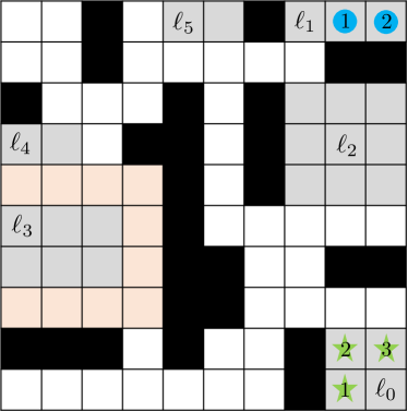
Figure 1: Illustration of the workspace for Example 1.

Example 1 (Valid temporal logic tasks)

Consider a mail delivery task amidst the COVID-19 pandemic (shown in Fig. 1) where three robots of type 1 (green stars) and two robots of type 2 (blue circles) are located at region $\ell_{0}$ and $\ell_{1}$, respectively, $\ell_{2}$ is an office building that the robots visit to pick up the mail, $\ell_{3}$ and $\ell_{5}$ are two delivery sites, and $\ell_{4}$ is a control room from where other robots are driven to the orange area between $\ell_{3}$ and $\ell_{4}$ to get disinfected and then drop off the mail at the delivery site $\ell_{3}$. We consider two delivery tasks: (i) Two robots of type 1 visit building $\ell_{2}$ to collaboratively pick up the mail and deliver it to the delivery site $\ell_{3}$, and one robot of type 2 must visit the control room $\ell_{4}$ to disinfect robots of type 1 before they get to the delivery site $\ell_{3}$. (ii) One robot of type 1 travels between building $\ell_{2}$ and the delivery site $\ell_{3}$ back and forth to transport equipment, assuming that the disinfection area operates automatically after task (i). These tasks are more complex than typical task allocation problems due to the temporal operators like “before” and “back and forth”. Observe that in Fig. 1, the atomic propositions satisfied by initial robot locations are $\mathcal{\pi}_{{3},{1}}^{0}$ and $\mathcal{\pi}_{{2},{2}}^{1}$. Moreover, tasks (i) and (ii) can be captured by the valid formulas $\phi_{1}=\lozenge\left(\left(\mathcal{\pi}_{{2},{1}}^{2,1}\wedge\neg\mathcal{\pi}_{{2},{1}}^{3}\right)\wedge\lozenge\mathcal{\pi}_{{2},{1}}^{3,1}\right)\wedge\lozenge\mathcal{\pi}_{{1},{2}}^{4}\wedge\neg\mathcal{\pi}_{{2},{1}}^{3}\,\mathcal{U}\,\mathcal{\pi}_{{1},{2}}^{4}$ and $\phi_{2}=\square\lozenge\left(\mathcal{\pi}_{{1},{1}}^{2,1}\wedge\lozenge\mathcal{\pi}_{{1},{1}}^{3,1}\right)$, respectively. Note that when binding the truth of atomic propositions, the value of $\chi$ is immaterial as long as it is the same non-zero number. Therefore, $\phi_{2}$ can also be written as $\square\lozenge\left(\mathcal{\pi}_{{1},{1}}^{2,2}\wedge\lozenge\mathcal{\pi}_{{1},{1}}^{3,2}\right)$. However, formulas $\lozenge\left(\mathcal{\pi}_{{1},{1}}^{2,1}\wedge\lozenge\mathcal{\pi}_{{2},{1}}^{3,1}\right)$ and $\lozenge\left(\mathcal{\pi}_{{2},{2}}^{2,1}\wedge\lozenge\mathcal{\pi}_{{2},{1}}^{3,1}\right)$ are two invalid formulas as they connect different numbers of robots $i$ and robot types $j$, respectively.

Let $s^{t}$ be the collective state at time $t$. A path of length $h$ is defined as $\tau=s^{0}\ldots s^{h}$ and it captures the collective behavior of the team such that $s^{t-1}\to s^{t},\forall t\in[h]$. Given a valid LTL${}^{\chi}$ formula $\phi$, a path $\tau=\tau^{\text{pre}}[\tau^{\text{suf}}]^{\omega}$ in a prefix-suffix structure that satisfies $\phi$ exists since there exists an accepting run in prefix-suffix form, where the prefix part $\tau^{\text{pre}}=s^{0}\dots s^{h_{1}}$ is executed once followed by the indefinite execution of the suffix part $\tau^{\text{suf}}=s^{h_{1}}\dots s^{h_{1}+h_{2}}s^{h_{1}+h_{2}+1}$, where $s^{h_{1}+h_{2}+1}=s^{h_{1}}$ [baier2008principles]. We say that a path $\tau$ satisfies $\phi$ if (a) the trace, defined as $\texttt{trace}(\tau):=L(s^{0})\dots L(s^{h_{1}})[L(s^{h_{1}})\dots L(s^{h_{1}+h_{2}+1})]^{\omega}$, belongs to $\texttt{Words}(\phi^{0})$, where $\phi^{0}$ is obtained by replacing all induced atomic propositions in $\phi$ by their counterparts with the zero connector and (b) it is the same $\langle i,j\rangle$ that satisfy the induced atomic propositions $\mathcal{\pi}_{{i},{j}}^{k,\chi}$ in $\phi$ sharing the same nonzero connector $\chi$. In other words, condition (a) restricts the label of the path, while condition (b) restricts the robots that participate in the satisfaction of induced atomic propositions. If $\phi\in\textup{LTL}^{0}$, the satisfaction conditions only include (a).

III-C Problem definition

Given a path $\tau_{r,j}=s_{r,j}^{0},s_{r,j}^{1},\ldots,s_{r,j}^{h}$ of length $h$ for robot $[r,j]$, we define the cost of $\tau_{r,j}$ as $J(\tau_{r,j})=\sum_{t=0}^{h-1}d(s_{r,j}^{t},s_{r,j}^{t+1})$, where $d:S\times S\to\mathbb{R}^{+}\cup\{0\}$ is a cost function that maps a pair of free cells to a non-negative value, for instance, travel distance or time. The cost of path $\tau$ that combines all robot paths $\tau_{r,j}$ of length $h$ is given by

$$J(\tau)=\sum_{{r\in{\mathcal{K}}_{j},j\in[m]}}J(\tau_{r,j}).$$ (1)

For plans written in prefix-suffix form, we get

$$J(\tau)=\beta J(\tau^{\text{pre}})+(1-\beta)J(\tau^{\text{suf}}),$$ (2)

where $\beta\in[0,1]$ is a user-specified parameter. Then, the problem addressed in this paper can be formulated as follows.

Problem 1

Consider a discrete workspace with labeled regions and obstacles, a team of $n$ robots of $m$ types, and a valid formula $\phi\in\textit{LTL}^{\chi}$. Plan a path for each robot such that the specification $\phi$ is satisfied and the cost in (2) is minimized.

We refer to Problem 1 as the Multi-Robot Task Allocation problem under LTL specifications or LTL-MRTA. This is a single-task robot and multi-robot task (ST-MR) problem, where a robot is capable of one task and a task may require multiple robots. Since the ST-MR problem is NP-hard [korsah2013comprehensive, nunes2017taxonomy], so is the LTL-MRTA problem. Consequently, existing approaches to this problem become intractable for large-scale applications [sahin2017provably, sahin2017synchronous]. In this work, we propose a new hierarchical framework to solve LTL-MRTA problems efficiently.

III-D Assumptions

In this section, we discuss assumptions on the workspace and the NBA translated from the LTL specifications that are necessary to ensure completeness of our propose hierarchical framework. As we discuss later in Section VII, these assumptions are mild and were satisfied by all tasks we tested our method on, regardless of their complexity.

III-D1 Workspace

The following assumption ensures that regions in the workspace are well-defined and mutually exclusive.

Assumption III.5 (Workspace)

Regions are disjoint, and each region spans consecutive cells. There exists a label-free path between any two regions, between any two label-free cells, and between any label-free cells and any regions.

If regions are partially overlapping or span multiple clusters of cells, we can define additional atomic propositions to satisfy Assumption III.5. Assumption III.5 implies that there are no “holes” inside regions that generate different labels, label-free cells are connected, and each region is adjacent to a label-free cell.

III-D2 Nondeterministic B$\ddot{\text{u}}$chi Automaton (NBA)

Given a team of $n$ robots and an LTL${}^{\chi}$ formula $\phi$, we can find a path $\tau$ that satisfies $\phi$ by operating on the corresponding NBA ${\mathcal{A}}_{\phi}=({\mathcal{V}},{\mathcal{E}})$, which can be constructed using existing tools, such as LTL2BA developed by [gastin2001fast]; see also Fig. 2 for the NBA of tasks (i) and (ii). Note that the NBA in Definition II.1 is essentially a graph. Thus, in the remainder of this paper, we refer to the NBA by the graph ${\mathcal{A}}_{\phi}$ for notational convenience. Before we discuss our assumptions on the structure of the NBA ${\mathcal{A}}_{\phi}$, we describe a list of pre-processing steps to obtain an ”equivalent” NBA that does not lose any feasible paths that satisfy the specification $\phi$. The goal is to remove infeasible and redundant transitions in the NBA to reduce its size.

Specifically, let the propositional formula $\gamma\in\Sigma$ associated with every transition $v_{1}\xrightarrow{\gamma}v_{2}$ in the NBA ${\mathcal{A}}_{\phi}$ be in disjunctive normal form (DNF), i.e, $\gamma=\bigvee_{p\in{\mathcal{P}}}\bigwedge_{q\in{\mathcal{Q}}_{p}}(\neg)\mathcal{\pi}_{{i},{j}}^{k,\chi}$, where the negation operator can only precede the atomic propositions and ${\mathcal{P}}$ and ${\mathcal{Q}}_{p}$ are proper index sets. Note that any propositional formula has an equivalent formula in DNF [baier2008principles]. We call ${\mathcal{C}}_{p}^{\gamma}=\bigwedge_{q\in{\mathcal{Q}}_{p}}(\neg)\mathcal{\pi}_{{i},{j}}^{k,\chi}$ the $p$-th clause of $\gamma$ that includes a set ${\mathcal{Q}}_{p}$ of positive and negative literals and each positive literal is an atomic proposition $\mathcal{\pi}_{{i},{j}}^{k,\chi}\in{\mathcal{A}}{\mathcal{P}}$. Let $\mathsf{cls}(\gamma)$ denote the set of clauses ${\mathcal{C}}_{p}^{\gamma}$ in $\gamma$. And let $\mathsf{lits}^{+}({\mathcal{C}}_{p}^{\gamma})$ and $\mathsf{lits}^{-}({\mathcal{C}}_{p}^{\gamma})$ be the positive subformula and negative subformula, consisting of all positive literals and all negative literals in the clause ${\mathcal{C}}_{p}^{\gamma}$. Those subformulas are $\top$ (constant true) if the corresponding literals do not exist. In what follows, we do not consider self-loops when we refer to edges in ${\mathcal{A}}_{\phi}$, since self-loops can be captured by vertices. We call the propositional formula $\gamma$ a vertex label if $v_{1}=v_{2}$, otherwise, an edge label. With a slight abuse of notation, let $\gamma:{\mathcal{V}}\to\Sigma$ and $\gamma:{\mathcal{V}}\times{\mathcal{V}}\to\Sigma$ be the functions that map a vertex and edge in the NBA to its vertex label and edge label, respectively. Given an edge $(v_{1},v_{2})$, we call labels $\gamma(v_{1})$ and $\gamma(v_{2})$ the starting and end vertex labels, respectively. Next, we pre-process the NBA ${\mathcal{A}}_{\phi}$ by removing infeasible clauses and merging redundant literals. In particular, given a vertex or edge label $\gamma$ in ${\mathcal{A}}_{\phi}$ we perform the following operations:

(1) Absorption in $\mathsf{lits}^{+}({\mathcal{C}}_{p}^{\gamma})$: For each clause ${\mathcal{C}}_{p}^{\gamma}\in\mathsf{cls}(\gamma)$, we delete the positive literal $\mathcal{\pi}_{{i},{j}}^{k}\in\mathsf{lits}^{+}({\mathcal{C}}_{p}^{\gamma})$, replacing it with $\top$, if another $\mathcal{\pi}_{{i^{\prime}},{j}}^{k,\chi^{\prime}}\in\mathsf{lits}^{+}({\mathcal{C}}_{p}^{\gamma})$ exists such that $i\leq i^{\prime}$. This is because if $\langle i^{\prime},j\rangle$ are at region $\ell_{k}$, i.e., $\mathcal{\pi}_{{i^{\prime}},{j}}^{k,\chi^{\prime}}$ is true, so is $\mathcal{\pi}_{{i},{j}}^{k}$. Similarly, we replace $\mathcal{\pi}_{{i},{j}}^{k}$ by $\mathcal{\pi}_{{i-i^{\prime}},{j}}^{k}$ if $i>i^{\prime}$, since $i-i^{\prime}$ additional robots are needed to make $\mathcal{\pi}_{{i},{j}}^{k}$ true if $\mathcal{\pi}_{{i^{\prime}},{j}}^{k,\chi^{\prime}}$ is true.

(2) Absorption in $\mathsf{lits}^{-}({\mathcal{C}}_{p}^{\gamma})$: We delete the negative literal $\neg\mathcal{\pi}_{{i},{j}}^{k}\in\mathsf{lits}^{-}({\mathcal{C}}_{p}^{\gamma})$, if another $\neg\mathcal{\pi}_{{i^{\prime}},{j}}^{k}\in\mathsf{lits}^{-}({\mathcal{C}}_{p}^{\gamma})$ exists such that $i^{\prime}<i$. This is because if $\neg\mathcal{\pi}_{{i^{\prime}},{j}}^{k}$ is true, so is $\neg\mathcal{\pi}_{{i},{j}}^{k}$.

(3) Mutual exclusion in $\mathsf{lits}^{+}({\mathcal{C}}_{p}^{\gamma})$: We delete the clause ${\mathcal{C}}_{p}^{\gamma}\in\mathsf{cls}(\gamma)$, replacing it with constant false $\bot$, if there exist two positive literals $\mathcal{\pi}_{{i},{j}}^{k,\chi},\mathcal{\pi}_{{i},{j}}^{k^{\prime},\chi}\in\mathsf{lits}^{+}({\mathcal{C}}_{p}^{\gamma})$ such that $k\not=k^{\prime}$ and $\chi\not=0$. The reason is that the same $i$ robots of type $j$ cannot be at different regions at the same time.

(4) Mutual exclusion in $\mathsf{lits}^{+}({\mathcal{C}}_{p}^{\gamma})$ and $\mathsf{lits}^{-}({\mathcal{C}}_{p}^{\gamma})$: We delete the clause ${\mathcal{C}}_{p}^{\gamma}\in\mathsf{cls}(\gamma)$ if there exists a positive literal $\mathcal{\pi}_{{i},{j}}^{k,\chi}\in\mathsf{lits}^{+}({\mathcal{C}}_{p}^{\gamma})$ and a negative literal $\neg\mathcal{\pi}_{{i^{\prime}},{j}}^{k}\in\mathsf{lits}^{-}({\mathcal{C}}_{p}^{\gamma})$ such that $i^{\prime}\leq i$. This is because these literals are mutually exclusive.

(5) Violation of team size: For each clause ${\mathcal{C}}_{p}^{\gamma}\in\mathsf{cls}(\gamma)$, let $\mathsf{lits}^{+}(j^{\prime})$ denote literals in $\mathsf{lits}^{+}({\mathcal{C}}_{p}^{\gamma})$ that involve robots of type $j^{\prime}$, i.e., $\mathsf{lits}^{+}(j^{\prime})=\{\mathcal{\pi}_{{i},{j}}^{k,\chi}\in\mathsf{lits}^{+}({\mathcal{C}}_{p}^{\gamma})|j=j^{\prime}\}$. We delete the clause ${\mathcal{C}}_{p}^{\gamma}$ if the total required number of robots of type $j$ exceeds the size $|{\mathcal{K}}_{j}|$, i.e., if there exists $j\in[m]$ such that $\sum_{\mathcal{\pi}_{{i},{j}}^{k,\chi}\in\mathsf{lits}^{+}(j)}i>|{\mathcal{K}}_{j}|$.

Note that these pre-processing steps merely remove infeasible clauses and merge redundant literals in the NBA ${\mathcal{A}}_{\phi}$, and they do compromise any accepting words in ${\mathcal{L}}({\mathcal{A}}_{\phi})$ that can be generated by a feasible path. Therefore, with a slight abuse of notation, we continue to use ${\mathcal{A}}_{\phi}$ to refer to the NBA associated with formula $\phi$ that is obtained after these pre-processing steps.

Consider now an edge $e=(v_{1},v_{2})$ and its starting vertex $v_{1}$ in the NBA ${\mathcal{A}}_{\phi}$ and assume that the current state of ${\mathcal{A}}_{\phi}$ is vertex $v_{1}$. For the NBA to transition to vertex $v_{2}$, certain robots need to simultaneously reach certain regions or avoid certain regions in order to make $\gamma(v_{1},v_{2})$ true, while maintaining $\gamma(v_{1})$ true en route. We assume that the transition to $v_{2}$ occurs immediately once $\gamma(v_{1},v_{2})$ becomes true. Therefore, we can define by a subtask the set of actions that need to be taken by a group of robots in order to activate a transition in the NBA. Formally, we have the following definition.

Definition III.6 (Subtask)

Given an edge $(v_{1},v_{2})$ in the NBA ${\mathcal{A}}_{\phi}$, a subtask is defined by the associated edge label $\gamma(v_{1},v_{2})$ and starting vertex label $\gamma(v_{1})$.

Subtasks can be viewed as generalized reach-avoid tasks where specific types of robots should visit or avoid certain regions (the “reach” part of the tasks) while satisfying the starting vertex labels along the way (the “avoid” part of the tasks, which here is defined in a more general way compared to the conventional definition that requires robots to stay away from given regions in space).

Note that every accepting run defined in Section II-A consists of a sequence of subtasks, as they are defined in Definition III.6. However, not all sequences of subtasks associated with an accepting run make progress towards accomplishing the task. In what follows, we restrict the accepting runs in an NBA to those that make progress towards accomplishing the task. But first, we provide some intuition using the following example.

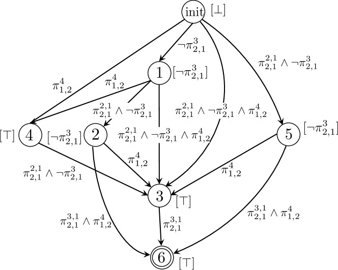
(a) NBA ${\mathcal{A}}_{\phi}$ for the task (i)

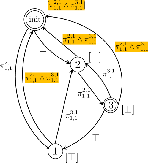
(b) NBA ${\mathcal{A}}_{\phi}$ for the task (ii)

Figure 2: NBA ${\mathcal{A}}_{\phi}$ for tasks (i) and (ii), where self-loops are omitted and the corresponding vertex labels are placed in square brackets.

Example 1

continued (Subtask progress in the pre-processed NBA ${\mathcal{A}}_{\phi}$) The pre-processed NBAs corresponding to tasks (i) and (ii) are shown in Fig. 2 where the vertex labels are placed in square brackets next to each vertex. After pre-processing, the NBA ${\mathcal{A}}_{\phi}$ for task (i) does not change whereas some labels in the NBA ${\mathcal{A}}_{\phi}$ for task (ii) become $\bot$ due to step (3). These labels are highlighted in orange.

In Fig. 2(a), $v_{\textup{init}}$ is the initial vertex and $v_{6}$ is the accepting vertex. Observe that all vertices have self-loops except for the initial vertex $v_{\textup{init}}$. In each accepting run, e.g., $v_{\textup{init}},v_{1},v_{2},v_{3},v_{6},v_{6}^{\omega}$, the satisfaction of an edge label leads to the satisfaction of its end vertex label, assuming this end vertex label is not $\bot$. For instance, label $\mathcal{\pi}_{{2},{1}}^{2,1}\wedge\neg\mathcal{\pi}_{{2},{1}}^{3}$ of edge $(v_{1},v_{2})$ implies label $\neg\mathcal{\pi}_{{2},{1}}^{3}$ of vertex $v_{2}$, and label $\neg\mathcal{\pi}_{{2},{1}}^{3}$ of edge $(v_{\textup{init}},v_{1})$ implies label $\neg\mathcal{\pi}_{{2},{1}}^{3}$ of its end vertex $v_{1}$. Intuitively, the completion of a subtask indicated by the satisfaction of its edge label, automatically activates the subtasks that immediately follow it indicated by the satisfaction of their starting vertex labels. This is because once the edge is enabled, its end vertex label should be satisfied at the next time instant; otherwise, progress in the NBA ${\mathcal{A}}_{\phi}$ will get stuck. The same observation also applies to the NBA in Fig. 2(b) where the vertex $v_{\textup{init}}$ is both an initial and accepting vertex and $v_{3}$ is another accepting vertex. The accepting run $v_{\textup{init}},v_{2},v_{3},(v_{1},v_{2},v_{3})^{\omega}$ includes one pair of initial and accepting vertices, $v_{\textup{init}}$ and $v_{3}$, and the accepting run $v_{\textup{init}},v_{2},v_{1},v_{\textup{init}}^{\omega}$ (although infeasible) includes one pair of initial and accepting vertices, $v_{\textup{init}}$ and $v_{\textup{init}}$. Note that we view the two $v_{\textup{init}}$ vertices differently, one as the initial vertex and the other as the accepting vertex. Furthermore, label $\mathcal{\pi}_{{1},{1}}^{3,1}$ of edge $(v_{1},v_{2})$ implies label $\top$ of its end vertex $v_{2}$; the same holds for the edge $(v_{2},v_{\textup{init}})$ and its end vertex $v_{\textup{init}}$ (although infeasible). It is noteworthy that even though the accepting vertex $v_{3}$ does not have a self-loop, the satisfaction of the label $\mathcal{\pi}_{{1},{1}}^{2,1}$ of its incoming edge $(v_{2},v_{3})$ leads to the satisfaction of the label $\top$ of its outgoing edge $(v_{3},v_{1})$. If the satisfaction of the incoming edge label does not imply satisfaction of the outgoing edge label, then progress in the NBA will get stuck at $v_{3}$ since the label $\mathcal{\pi}_{{1},{1}}^{2,1}\wedge\mathcal{\pi}_{{1},{1}}^{3,1}$ of edge $(v_{3},v_{\textup{init}})$ is infeasible and the transition between regions $\ell_{2}$ and $\ell_{3}$ requires more than one time steps; see Fig. 1, which makes the label $\mathcal{\pi}_{{1},{1}}^{3,1}$ of edge $(v_{3},v_{2})$ unsatisfiable at the next time instant.

Motivated by the observations in Example 1, we introduce the notions of implication and strong implication between two propositional formulas. Then, we define a restricted accepting run in the NBA ${\mathcal{A}}_{\phi}$ in a prefix-suffix structure. The completeness of our method relies on the assumption that the set of restricted accepting runs in the NBA ${\mathcal{A}}_{\phi}$ is nonempty.

Definition III.7 (Implication and strong implication)

Given two propositional formulas $\gamma$ and $\gamma^{\prime}$ over ${\mathcal{A}}{\mathcal{P}}$, we say that formula $\gamma$ implies $\gamma^{\prime}$, denoted by $\gamma\Longrightarrow\gamma^{\prime}$, if for each clause ${\mathcal{C}}_{p}^{\gamma}\in\mathsf{cls}(\gamma)$, there exists a clause ${\mathcal{C}}_{p^{\prime}}^{\gamma^{\prime}}\in\mathsf{cls}(\gamma^{\prime})$ such that ${\mathcal{C}}_{p^{\prime}}^{\gamma^{\prime}}$ is a subformula of ${\mathcal{C}}_{p}^{\gamma}$, i.e., all literals in ${\mathcal{C}}_{p^{\prime}}^{\gamma^{\prime}}$ also appear in ${\mathcal{C}}_{p}^{\gamma}$. By default, $\top$ is a subformula of any clause. In addition, formula $\gamma$ strongly implies $\gamma^{\prime}$, denoted by $\gamma\Longrightarrow_{s}\gamma^{\prime}$, if $\gamma\Longrightarrow\gamma^{\prime}$, and for each clause ${\mathcal{C}}_{p^{\prime}}^{\gamma^{\prime}}\in\mathsf{cls}(\gamma^{\prime})$, there exists a clause ${\mathcal{C}}_{p}^{\gamma}\in\mathsf{cls}(\gamma)$ such that ${\mathcal{C}}_{p^{\prime}}^{\gamma^{\prime}}$ is a subformula of ${\mathcal{C}}_{p}^{\gamma}$.

Intuitively, if $\gamma\Longrightarrow\gamma^{\prime}$ or $\gamma\Longrightarrow_{s}\gamma^{\prime}$, robot locations that satisfy $\gamma$ also satisfy $\gamma^{\prime}$.

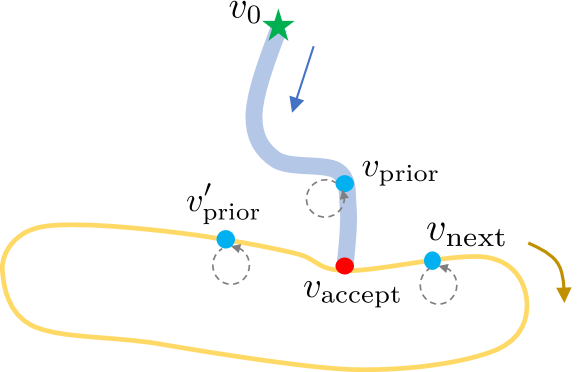
Figure 3: Graphical depiction of the accepting run in the prefix-suffix structure when $v_{\textup{accept}}$ does not have a self-loop, which resembles a lasso. The shaded blue line and the orange loop represent the prefix and suffix part, respectively. The arrow indicates the progression direction and the gray circles indicate the self-loops.

Definition III.8 (Restricted accepting run)

Given the NBA ${\mathcal{A}}_{\phi}$ (after pre-processing) corresponding to an LTL${}^{\chi}$ formula, we call any accepting run in a prefix-suffix structure $\rho=\rho^{\textup{pre}}[\rho^{\textup{suf}}]^{\omega}=v_{0},\ldots,v_{\textup{prior}},v_{\textup{accept}}[v_{\textup{next}},\ldots,v_{\textup{prior}}^{\prime},v_{\textup{accept}}]^{\omega}$ (see Fig. 3), a restricted accepting run, if it satisfies the following conditions:

• If a vertex is both an initial vertex $v_{0}$ and an accepting vertex $v_{\textup{accept}}$, we treat it as two different vertices, namely an initial vertex and an accepting vertex. The accepting vertex $v_{\textup{accept}}$ appears only once at the end in both the prefix and suffix parts. In the prefix part $v_{0},\ldots,v_{\textup{prior}},v_{\textup{accept}}$, if a vertex appears multiple times, all repetitive occurrences are consecutive. The same holds for the suffix part $v_{\textup{next}},\ldots,v_{\textup{prior}}^{\prime},v_{\textup{accept}}$;

• There only exist one initial vertex $v_{0}$ and one accepting vertex $v_{\textup{accept}}$ in the accepting run (they can appear multiple times in a row). Different accepting runs can have different pairs of initial and accepting vertices;

• In the prefix part, only initial and accepting vertices, $v_{0}$ and $v_{\textup{accept}}$, are allowed not to have self-loops, i.e., their vertex labels can be $\bot$. In the suffix part, only the accepting vertex $v_{\textup{accept}}$ is allowed not to have a self-loop;

• For any two consecutive vertices $v_{1}$, $v_{2}$ in the accepting run $\rho$, if $v_{1}\neq v_{2}$, $v_{2}\neq v_{\textup{accept}}$ and $v_{2}$ has a self-loop, then the edge label $\gamma(v_{1},v_{2})$ strongly implies the end vertex label $\gamma(v_{2})$, i.e., $\gamma(v_{1},v_{2})\Longrightarrow_{s}\gamma(v_{2})$;

• In the suffix part $\rho^{\textup{suf}}$, if $v_{\textup{accept}}=v_{\textup{next}}$ (this happens when $v_{\textup{accept}}$ has a self-loop), then $\rho^{\textup{suf}}$ only contains the vertex $v_{\textup{accept}}$. Meanwhile, the label of the edge $(v_{\textup{prior}},v_{\textup{accept}})$ implies the label of the vertex $v_{\textup{accept}}$, i.e., $\gamma(v_{\textup{prior}},v_{\textup{accept}})\Longrightarrow\gamma(v_{\textup{accept}})$;

• In the suffix part, if $v_{\textup{accept}}\neq v_{\textup{next}}$ (this can happen when $v_{\textup{accept}}$ does not have a self-loop), then the label of the edge $(v_{\textup{prior}},v_{\textup{accept}})$ implies the label of the edge $(v_{\textup{accept}},v_{\textup{next}})$, i.e., $\gamma(v_{\textup{prior}},v_{\textup{accept}})\Longrightarrow\gamma(v_{\textup{accept}},v_{\textup{next}})$. Also, the label $\gamma(v_{\textup{prior}},v_{\textup{accept}})$ implies the label of the edge $(v_{\textup{prior}}^{\prime},v_{\textup{accept}})$, i.e., $\gamma(v_{\textup{prior}},v_{\textup{accept}})\Longrightarrow\gamma(v_{\textup{prior}}^{\prime},v_{\textup{accept}})$. Note that $v_{\textup{prior}}$ and $v_{\textup{prior}}^{\prime}$ can be different.

In what follows, we discuss the conditions in Definition III.8 in more detail. Specifically, conditions (a) and (b) require that a restricted accepting run is “simple”. Specifically, condition (a) states that vertices $v_{0}$ and $v_{\textup{accept}}$ can be treated differently since they mark different progress towards accomplishing a task. The prefix and suffix parts of a restricted accepting run end once $v_{\textup{accept}}$ is reached, as in [smith2010optimal]. By aggregating consecutive identical vertices in the prefix part of a restricted accepting run into one single vertex, there are no identical vertices in the “compressed” prefix part. That is, it contains no cycles. The presence of a cycle is redundant since it implies negative progress towards accomplishing the task. The same applies to the suffix part. On the other hand, condition (b) states that a restricted accepting run is basically an accepting run defined in Section II-A that is further defined over a pair of initial and accepting vertices. In Section IV, we extract smaller sub-NBAs from the NBA ${\mathcal{A}}_{\phi}$ for each pair of initial and accepting vertices, which helps reduce complexity of the problem.

Conditions (c)-(f) require that the completion of a subtask in a restricted accepting run automatically activates the subtasks that immediately follow it; see Example 1. This ensures that robots are given adequate time to undertake subsequent subtasks after completing the current subtask. Accepting runs that do not satisfy conditions (c)-(d) are disregarded. In fact, in Section IV-A we prune vertices and edges in the NBA that violate these conditions, further reducing the size of the NBA. Finally, the implication $\gamma(v_{\textup{prior}},v_{\textup{accept}})\Longrightarrow\gamma(v_{\textup{accept}},v_{\textup{next}})$ in condition (f) requires that the robot locations enabling the last edge in the prefix part of a restricted accepting run also enable the first edge in the suffix part. As a result, we can find the prefix and suffix parts of a restricted accepting run separately. Otherwise, the progress in the NBA ${\mathcal{A}}_{\phi}$ may get stuck since these two edge labels need to be satisfied at two consecutive time instants, similar to conditions (d) and (e). Also, as the suffix part of a restricted accepting run is a loop, robots need to return to their initial locations in the suffix part after executing the suffix part once. The relation $\gamma(v_{\textup{prior}},v_{\textup{accept}})\Longrightarrow\gamma(v_{\textup{prior}}^{\prime},v_{\textup{accept}})$ requires that the initial locations in the suffix part of a restricted accepting run enable the edge $(v_{\textup{prior}}^{\prime},v_{\textup{accept}})$, which ensures that the robots can travel back to the initial locations in the suffix part and, as a result, activate the transition in ${\mathcal{A}}_{\phi}$ back to the vertex $v_{\textup{accept}}$ that allows to repeat the suffix part $\rho^{\text{suf}}$. Finally, we make the following assumption on the structure of the NBA ${\mathcal{A}}_{\phi}$.

Assumption III.9 (Existence of restricted accepting runs)

The set of restricted accepting runs in the NBA ${\mathcal{A}}_{\phi}$ is non-empty.

We note that the sets of restricted accepting runs for tasks (i) and (ii) satisfy Assumption III.9. Common robotic tasks, such as sequencing and coverage, have NBAs that contain restricted accepting runs. However, there is also a small subclass of LTL where the “next” operator directly precedes an atomic proposition that violates this assumption. For instance, $\lozenge(\pi_{1,1}^{2,1}\wedge\bigcirc\pi_{1,2}^{3,1})$ requires a second robot to visit region $\ell_{3}$ immediately after the first robot reaches $\ell_{2}$, which does not allow for any physical time between the completion of the two consecutive subtasks. On the other hand, the LTL formula $\lozenge(\pi_{1,1}^{2,1}\wedge\bigcirc(\pi_{1,1}^{2,1}\mathcal{U}\pi_{2,1}^{3}))$ satisfies the assumption.

III-D3 Robot paths

The definition of restricted accepting runs is based entirely on the structure of the NBA and logical implication relations. However, Definition III.8 does not describe how to characterize robot paths that induce restricted accepting runs. In what follows, we discuss conditions under which robot paths satisfy restricted accepting runs. We call such paths satisfying paths and we assume that such satisfying paths exist.

Definition III.10 (Satisfying paths of restricted accepting runs)

Given a team of $n$ robots and a valid specification $\phi\in\textit{LTL}^{\chi}$, a robot path $\tau$ is a satisfying path that induces a restricted accepting run, if the following conditions hold:

• If a vertex label is satisfied by the path $\tau$, it is always satisfied by the same clause that is always satisfied by the same fleet of robots;

• If a clause in an edge label is satisfied by the path $\tau$, then a clause in the end vertex label is also satisfied. Moreover, the fleet of robots satisfying the positive subformula of the clause in the end vertex label is the same as the fleet of robots satisfying the positive subformula of the clause in the corresponding edge label;

• Robot locations enabling the edges $(v_{\textup{accept}},v_{\textup{next}})$ and $(v_{\textup{prior}}^{\prime},v_{\textup{accept}})$ in the suffix part of a restricted accepting run are identical to robot locations enabling the edge $(v_{\textup{prior}},v_{\textup{accept}})$ in the prefix part.

Definition III.10 is closely related to the definition of a restricted accepting run. Specifically, condition (a) in Definition III.10 requires that once a fleet of robots satisfies a vertex label in a restricted accepting run, then these robots remain idle during the next time instant so that the same clause in this vertex label is still satisfied. This satisfies condition (a) in Definition III.8. Furthermore, condition (b) in Definition III.10 requires that once a fleet of robots satisfies an edge label in a restricted accepting run, then these robots remain idle during the next time instant so that the clause in the end vertex label that is implied by the clause that is satisfied in the edge label is also satisfied. This satisfies condition (d) in Definition III.8.

Finally, condition (c) in Definition III.10 requires that the robot locations enabling the edge $(v_{\textup{prior}},v_{\textup{accept}})$ in the prefix part of a restricted accepting run coincide with the initial locations of the robots that enable the edge $(v_{\textup{prior}}^{\prime},v_{\textup{accept}})$ in the suffix part of the restricted accepting run, as per condition (f) in Definition III.8. Therefore, condition (c) in Definition III.10 requires that the robots travel along a loop so that the suffix part of the restricted accepting run is executed indefinitely. In what follows, we make the following assumption.

Assumption III.11 (Existence of satisfying paths)

There exist robot paths that satisfy the restricted accepting runs in the NBA ${\mathcal{A}}_{\phi}$.

III-E Outline of the proposed method

An overview of our proposed method is shown in Alg. 1, which first finds prefix paths and then suffix paths. The process of finding prefix or suffix paths consists of relaxation and correction stages. Specifically, during the relaxation stage, we ignore the negative literals in the NBA ${\mathcal{A}}_{\phi}$ and formulate a MILP to allocate subtasks to robots and determine time-stamped robot waypoints that satisfy the task assignment. To this end, we first prune the NBA ${\mathcal{A}}_{\phi}$ by deleting infeasible transitions and then relax it by removing negative subformulas so that transitions in the relaxed NBA are solely satisfied by robots that meet at certain regions [line 1]; see Section IV-A. The idea to temporarily remove negative literals from the NBA is motivated by “lazy collision checking” methods in robotics and allows to simplify the planning problem as the constraints are not considered during planning and are only checked during execution, when needed. Then, since by condition (b) in Definition III.8, restricted accepting runs contain only one initial vertex and one accepting vertex, for every sorted pair of initial and accepting vertices by length in the relaxed NBA, we extract a sub-NBA of smaller size [line 1]; see Section IV-B, where ${\mathcal{A}}_{\textup{subtask}}(v_{\textup{init}},v_{\textup{accept}})$ is the sub-NBA including only initial vertex $v_{\textup{init}}$, accept vertex $v_{\textup{accept}}$ and other intermediate vertices. The sub-NBAs are used to extract subtasks and temporal orders between them captured by a set of posets ([lines 1-1], see Section IV-C), and construct routing graphs, one for each poset, that capture the regions that the robots need to visit and the temporal order of the visits so that the subtasks extracted from the sub-NBAs are satisfied; see Section V-A. Finally, given the routing graph corresponding to each poset we formulate a MILP inspired by the vehicle routing problem to obtain a high-level task allocation plan along with time-stamped waypoints that the robots need to visit to satisfy the task assignment [lines 1-1]; see Section V-B. During the correction stage, we introduce the negative literals back into the NBA and formulate a collection of generalized multi-robot path planning problems, one for each poset, to design low-level executable robot paths that satisfy the original specification ([line 1], see Section V-C). Viewing the final states of the prefix paths as the initial states, a similar process is conducted for the sub-NBA ${\mathcal{A}}_{\textup{subtask}}(v_{\textup{accept}},v_{\textup{accept}})$ to find the suffix paths. Alg. 1 can terminate after a specific number of paths is found or all possible alternatives are explored. Under the mild assumptions discussed in Section III-D, completeness of our proposed method is shown in Theorem VI.1 in Section VI.

1

2Prune and relax the NBA ;

3 foreach sorted sub-NBA ${\mathcal{A}}_{\textup{subtask}}(v_{\textup{init}},v_{\textup{accept}})$  do

       ;

        $\triangleright$ Compute the prefix path

4       Prune the sub-NBA ${\mathcal{A}}_{\textup{subtask}}(v_{\textup{init}},v_{\textup{accept}})$;

5       Infer the set of posets $\{P_{\textup{pre}}\}$;

6       foreach sorted poset $P_{\textup{pre}}$ do

7             Build the routing graph ;

8             Formulate MILP to get prefix high-level plans ;

9             Formulate generalized multi-robot path planning to get prefix low-level paths ;

             ;

              $\triangleright$ Compute the suffix path

10             Prune the sub-NBA ${\mathcal{A}}_{\textup{subtask}}(v_{\textup{accept}},v_{\textup{accept}})$;

11             Infer the set of posets $\{P_{\textup{suf}}\}$;

12             foreach sorted poset $P_{\textup{suf}}$ do

13                   Build the routing graph;

14                   Formulate MILP to get suffix high-level plans;

15                   Formulate generalized multi-robot path planning to get suffix low-level paths;

16                  

Algorithm 1 Algorithm for LTL-MRTA

Remark III.12

We note that Assumption III.11 on the existence of satisfying paths is only a sufficient condition that needs to be satisfied to show completeness of our proposed method, as shown in the theoretical analysis of Section VI. The robot path returned by our method may not be a satisfying path, although it still satisfies the specification $\phi$.

IV Extraction of Subtasks from the NBA and Inferring their Temporal Order

In this section, we first prune and relax the NBA ${\mathcal{A}}_{\phi}$ by removing infeasible transitions and negative literals. As discussed before, this step is motivated by ”lazy collision checking” methods in robotics and allows to simplify the planning problem by checking constraint satisfaction during the execution of the plans rather than their synthesis. Then, we extract sub-NBAs from the relaxed NBA and use these sub-NBAs to obtain sequences of subtasks and a temporal order between them that need to be satisfied so that the global specification is satisfied.

IV-A Pruning and relaxation of the NBA

To prune infeasible transitions from the NBA ${\mathcal{A}}_{\phi}$, we first delete all edges labeled with $\bot$, as they cannot be enabled. We also delete vertices and edges in ${\mathcal{A}}_{\phi}$ that do not belong to restricted accepting runs, as defined in Definition III.8. Specifically, we delete all vertices without self-loops except for the initial and accepting vertices, as per condition (c) in Definition III.8. Furthermore, for every vertex other than the accepting vertex, we delete all its incoming edges with edge labels that do not strongly imply its vertex label, as per condition (d) in Definition III.8. Finally, we delete every vertex, except for the initial vertex, that cannot be reached by other vertices. We note that these pruning steps do not compromise any feasible solution to Problem 1 that induces a restricted accepting run in ${\mathcal{A}}_{\phi}$, as shown in Lemma LABEL:prop:prune in Appendix LABEL:app:correctness.

We denote by ${\mathcal{A}}_{\phi}^{-}$ the resulting pruned NBA. Given the pruned NBA ${\mathcal{A}}_{\phi}^{-}$, we further relax it by replacing each negative literal in vertex or edge labels with $\top$. Let ${\mathcal{A}}_{\textup{relax}}$ denote the relaxed NBA. Note that, when the specification $\phi$ does not involve negative atomic propositions, we have ${\mathcal{A}}_{\textup{relax}}={\mathcal{A}}_{\phi}^{-}$. Furthermore, Lemma LABEL:prop:inclusion in Appendix LABEL:app:correctness states that the language accepted by ${\mathcal{A}}_{\phi}^{-}$ is included in the language accepted by ${\mathcal{A}}_{\textup{relax}}$, so this relaxation step does not remove feasible solutions to Problem 1. In other words, ${\mathcal{A}}_{\textup{relax}}$ is an over-approximation of ${\mathcal{A}}_{\phi}^{-}$. However, a solution to Problem 1 based on ${\mathcal{A}}_{\textup{relax}}$ may not satisfy the specification $\phi$. Note that ${\mathcal{A}}_{\phi}^{-}$ and ${\mathcal{A}}_{\textup{relax}}$ are sub-NBAs of ${\mathcal{A}}_{\phi}$ in terms of vertices and edges. Thus, labels and runs in ${\mathcal{A}}_{\phi}^{-}$ and ${\mathcal{A}}_{\textup{relax}}$ can be mapped to labels and runs in ${\mathcal{A}}_{\phi}$. For instance, for an edge label $\gamma$ in ${\mathcal{A}}_{\textup{relax}}$, we denote by $\gamma_{\phi}$ the corresponding label in ${\mathcal{A}}_{\phi}$ (including negative literals).

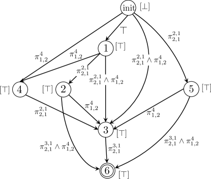
(a) ${\mathcal{A}}_{\textup{relax}}$ for task (i)

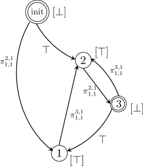
(b) ${\mathcal{A}}_{\textup{relax}}$ for task (ii)

Figure 4: The relaxed NBA ${\mathcal{A}}_{\textup{relax}}$ for tasks (i) and (ii).

Example 1

continued (Pruning and relaxation of the NBA ${\mathcal{A}}_{\phi}$) The pruned NBA ${\mathcal{A}}_{\phi}^{-}$ for the task (i) is the same as the original NBA in Fig. 2(a). The relaxed NBA ${\mathcal{A}}_{\textup{relax}}$ is shown in Fig. 4(a). The pruned NBA ${\mathcal{A}}_{\phi}^{-}$ for the task (ii) is the same as the relaxed NBA ${\mathcal{A}}_{\textup{relax}}$ which is shown in Fig. 4(b). Particularly, ${\mathcal{A}}_{\phi}^{-}$ is obtained from ${\mathcal{A}}_{\phi}$ in Fig. 2(b) by removing edges $(v_{1},v_{\textup{init}}),(v_{2},v_{\textup{init}}),(v_{3},v_{\textup{init}})$ and replacing $\gamma(v_{\textup{init}})$ with $\bot$.

IV-B Extraction of sub-NBA ${\mathcal{A}}_{\textup{subtask}}$ from ${\mathcal{A}}_{\textup{relax}}$

In this section, we extract multiple sub-NBAs from the relaxed NBA ${\mathcal{A}}_{\textup{relax}}$, one for every pair of initial and accepting vertices in ${\mathcal{A}}_{\textup{relax}}$. Then, in Section IV-C, we determine the temporal order among subtasks in every sub-NBA.

IV-B1 Sorting the pairs of initial and accepting vertices by path length

As required by condition (b) in Definition III.8, every restricted accepting run in ${\mathcal{A}}_{\textup{relax}}$ contains one pair of initial and accepting vertices. In what follows, we sort all pairs of initial and accepting vertices in ${\mathcal{A}}_{\textup{relax}}$ in an ascending order so that the pair of initial and accepting vertices connected by a restricted accepting run with the shortest length appears first. Then in Section IV-B2, we extract a sub-NBA from ${\mathcal{A}}_{\textup{relax}}$ for each pair in this ascending order. Intuitively, the sub-NBAs corresponding to restricted accepting runs of shorter length generally will contain fewer subtasks to be completed.

(a) Computation of the shortest simple prefix path

Given a pair of an initial vertex $v_{0}$ and an accepting vertex $v_{\textup{accept}}$ in ${\mathcal{A}}_{\textup{relax}}$, we first compute the shortest simple path from $v_{0}$ to $v_{\textup{accept}}$ in terms of the number of edges/subtasks, where a simple path does not contain any repeating vertices, as per condition (a) in Definition III.8 that excludes cycles from restricted accepting runs. This step corresponds to the prefix part of a restricted accepting run. To this end, we first remove all other initial vertices and accepting vertices from ${\mathcal{A}}_{\textup{relax}}$. This will not affect the restricted accepting runs in ${\mathcal{A}}_{\textup{relax}}$ associated with the pair $v_{0}$ and $v_{\textup{accept}}$ due to condition (b) in Definition III.8. Then, depending on whether the initial vertex $v_{0}$ has a self-loop, we proceed as follows.

(1) If $v_{0}$ does not have a self-loop, i.e., $\gamma(v_{0})=\bot$: We remove all outgoing edges $v_{0}$ in ${\mathcal{A}}_{\textup{relax}}$ with label $\gamma$, if the initial robot locations do not satisfy the corresponding edge label $\gamma_{\phi}$ (including the negative literals) in ${\mathcal{A}}_{\phi}$. We emphasize that we need to check satisfaction of $\gamma_{\phi}$ in the NBA ${\mathcal{A}}_{\phi}$ instead of satisfaction of $\gamma$ in the relaxed NBA ${\mathcal{A}}_{\textup{relax}}$, since if initial robot locations cannot enable an edge starting from $v_{0}$ in ${\mathcal{A}}_{\phi}$, there is no reason to consider this edge in any NBA.

(2) If $v_{0}$ has a self-loop, i.e., $\gamma(v_{0})\neq\bot$: We check whether the initial robot locations satisfy $\gamma_{\phi}(v_{0})$ in the NBA ${\mathcal{A}}_{\phi}$. If yes, we do nothing; otherwise, we proceed as in case (a) in this part and remove the self-loop of $v_{0}$ as well as all its outgoing edges in ${\mathcal{A}}_{\textup{relax}}$ if the initial robot locations do not satisfy the corresponding edge label $\gamma_{\phi}$ in ${\mathcal{A}}_{\phi}$.

Next, the shortest simple path connecting $v_{0}$ and $v_{\textup{accept}}$ can be found using Dijkstra’s algorithm. Note that if a vertex is both an initial and accepting vertex, we treat it once as the initial vertex and once as the accepting vertex, although it appears twice in the shortest simple path.

(b) Computation of the shortest simple suffix cycle

Next, we compute the shortest simple cycle around $v_{\text{accept}}$ in ${\mathcal{A}}_{\textup{relax}}$, where repeating vertices only appear at the beginning and at the end of the simple cycle. This step corresponds to the suffix part of a restricted accepting run, which is conducted in the original NBA ${\mathcal{A}}_{\textup{relax}}$. If $v_{\textup{accept}}$ in ${\mathcal{A}}_{\textup{relax}}$ has a self-loop, then the length of the shortest simple cycle is 0. Otherwise, similar to steps in Section (a) used to find the shortest simple prefix path, we first remove all other accepting vertices from ${\mathcal{A}}_{\textup{relax}}$ and then remove all initial vertices (including $v_{0}$) if they do no have self-loops. In this way, the only vertex that does not have a self-loop is the accepting vertex $v_{\textup{accept}}$. This will not affect those restricted accepting runs that are related to $v_{0}$ and $v_{\textup{accept}}$ due to conditions (b) and (c) in Definition III.8.

Finally, the length associated with the pair $v_{0}$ and $v_{\textup{accept}}$ is equal to the total length of the shortest simple prefix path and the shortest simple suffix cycle connecting these vertices in ${\mathcal{A}}_{\textup{relax}}$. By default, if no simple path or cycle exists for the pair $v_{0}$ and $v_{\textup{accept}}$, the length is infinite, which means there is no restricted accepting run for this pair. We repeat this process for all pairs of initial and accepting vertices in ${\mathcal{A}}_{\textup{relax}}$ and sort them in ascending order in terms of the total length. As discussed before, we plan first for pairs with shorter length since they contain fewer subtasks to be completed.

IV-B2 Extraction of the sub-NBA ${\mathcal{A}}_{\textup{subtask}}$

For every pair of vertices $v_{0}$ and $v_{\text{accept}}$ in ${\mathcal{A}}_{\textup{relax}}$ connected by a simple path of finite total length in the above ascending order, our goal is to determine time-stamped task allocation plans for all robots that induce the simple prefix path and simple suffix cycle in ${\mathcal{A}}_{\textup{relax}}$ connecting $v_{0}$ and $v_{\textup{accept}}$. To do this, we extract one sub-NBA from the NBA ${\mathcal{A}}_{\textup{relax}}$ that we can use to construct the prefix part of the plan and one that we can use to construct the suffix part of the plan, respectively. Here, we discuss the sub-NBA for the prefix part. The sub-NBA for the suffix part is similar and is discussed in Appendix LABEL:sec:suf.

Given the pair of vertices $v_{0}$ and $v_{\textup{accept}}$, we construct a prefix sub-NBA ${\mathcal{A}}_{\textup{subtask}}$ by the following three steps. First, we follow exactly the same steps in Section (a) that computes the shortest simple prefix path to prune the NBA ${\mathcal{A}}_{\textup{relax}}$. Next, we remove all outgoing edges from $v_{\textup{accept}}$ if $v_{\textup{accept}}\not=v_{0}$, because we focus on the prefix part. Finally, let ${\mathcal{V}}_{\text{s}}$ denote the set that contains all remaining vertices in ${\mathcal{A}}_{\textup{relax}}$ that belong to some path connecting $v_{0}$ and $v_{\textup{accept}}$. Then, we construct a sub-NBA ${\mathcal{A}}_{\textup{subtask}}=({\mathcal{V}}_{\text{s}},{\mathcal{E}}_{\text{s}})$ from ${\mathcal{A}}_{\textup{relax}}$ that includes all edges that connect the vertices in ${\mathcal{V}}_{\text{s}}$. The sub-NBA ${\mathcal{A}}_{\textup{subtask}}$ contains prefix parts of all restricted accepting runs associated with the pair $v_{0}$ and $v_{\textup{accept}}$.

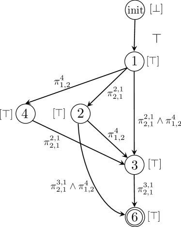
(a) ${\mathcal{A}}_{\textup{subtask}}$ for task (i)

(b) ${\mathcal{A}}_{\textup{subtask}}$ for task (ii)

Figure 5: Sub-NBA ${\mathcal{A}}_{\textup{subtask}}$ for the prefix part of tasks (i) and (ii) in Example 1, obtained from the NBA ${\mathcal{A}}_{\textup{relax}}$ in Fig. 4.

Example 1

continued (Sub-NBA ${\mathcal{A}}_{\textup{subtask}}$) The sub-NBA ${\mathcal{A}}_{\textup{subtask}}$ for the prefix parts of plans associated with tasks (i) and (ii) are shown in Fig. 5. For task (i), given the pair $v_{\textup{init}}$ and $v_{6}$ in the relaxed NBA ${\mathcal{A}}_{\textup{relax}}$ in Fig. 4(a), the total length is $3+0=3$ (edges $(v_{\textup{init}},v_{3}),(v_{\textup{init}},v_{4}),(v_{\textup{init}},v_{5})$ were removed since $v_{\textup{init}}$ does not have a self-loop and all robots initially located inside region $\ell_{1}$ do not satisfy their labels; see Fig. 1). The NBA ${\mathcal{A}}_{\textup{subtask}}$, shown in Fig. 5(a) is obtained by removing edges $(v_{\textup{init}},v_{3}),(v_{\textup{init}},v_{4}),(v_{\textup{init}},v_{5}),(v_{5},v_{3}),(v_{5},v_{6})$ and vertex $v_{5}$ from ${\mathcal{A}}_{\textup{relax}}$. For task (ii), given the pair $v_{\textup{init}}$ and $v_{\textup{init}}$, there is no cycle leading back to $v_{\textup{init}}$, so the total length is infinite and there is no corresponding sub-NBA ${\mathcal{A}}_{\textup{relax}}$. The total length for the pair $v_{\textup{init}}$ and $v_{3}$ is $2+2=4$. The NBA ${\mathcal{A}}_{\textup{subtask}}$ is shown in Fig. 5(b), where edges $(v_{\textup{init}},v_{1})$ and $(v_{1},v_{2})$ are removed since $v_{\textup{init}}$ does not have a self-loop and initial robot locations do not satisfy their labels.

Example 1

continued (Subtasks in ${\mathcal{A}}_{\textup{subtask}}$) The sub-NBA ${\mathcal{A}}_{\textup{subtask}}$ is composed of subtasks that need to be satisfied in specific orders to reach the accepting vertex. For instance, the path $v_{\textup{init}},v_{1},v_{4},v_{3},v_{6}$ in Fig. 4(a) requires that first $\langle 1,2\rangle$ visits the control room $\ell_{4}$, then $\langle 2,1\rangle$ visit the office building $\ell_{2}$ and finally the same two robots of type 1 drop off the mail at the delivery site $\ell_{3}$. By definition of task (i), the temporal order between these subtasks specifies that the time when $\langle 1,2\rangle$ visits the control room $\ell_{4}$ is independent from the time when $\langle 2,1\rangle$ pick up the mail at the building $\ell_{2}$, and that $\langle 1,2\rangle$ visiting $\ell_{4}$ and $\langle 2,1\rangle$ visiting $\ell_{2}$ should occur prior to $\langle 2,1\rangle$ visiting the delivery site $\ell_{3}$.

IV-B3 Pruning the sub-NBA ${\mathcal{A}}_{\textup{subtask}}$

Observe that the sub-NBA ${\mathcal{A}}_{\textup{subtask}}$ in Fig. 5(a) still constitutes a large portion of ${\mathcal{A}}_{\textup{relax}}$ in Fig. 4(a), which is common in practice, since there are typically many more edges than vertices in ${\mathcal{A}}_{\textup{relax}}$. However, some edges/subtasks are “redundant” in that they can be decomposed into more elementary edges/subtasks. Therefore, in what follows, we further prune the NBA ${\mathcal{A}}_{\textup{subtask}}$ by removing such redundant edges.

Recall Definition III.6 where subtasks are defined by their edge labels and starting vertex labels. Next we define the notion of equivalent subtasks.

Definition IV.1 (Equivalent subtasks)

Subtasks $(v_{1},v_{2})$ and $(v^{\prime}_{1},v^{\prime}_{2})$ in an NBA ${\mathcal{A}}_{\textup{}}$ are equivalent, denoted by $(v_{1},v_{2})\sim(v^{\prime}_{1},v^{\prime}_{2})$, if $\gamma(v_{1})=\gamma(v^{\prime}_{1})$, $\gamma(v_{1},v_{2})=\gamma(v_{1}^{\prime},v^{\prime}_{2})$ and they are not in the same path that connects the same pair of initial and accepting vertices.

The last condition in Definition IV.1 is necessary since two subtasks in the same path mark different progress towards completing a task, even if they have identical labels. Recall that in task (i) in Example 1, certain regions can be visited in parallel. To capture the parallel visits, we define the following two properties over vertices in ${\mathcal{A}}_{\textup{subtask}}$, namely, the independent diamond (ID) property adapted from [stefanescu2006automatic] and the sequential triangle (ST) property over vertices; see also Fig. 6.

Definition IV.2 (Independent diamond property)

Given four different vertices $v_{1},v_{2},v_{3},v_{4}$ in the NBA ${\mathcal{A}}_{\textup{subtask}}$, we say that these four vertices satisfy the ID property if

• $\gamma(v_{1})=\gamma(v_{2})=\gamma(v_{4})$;

• $v_{1}\xrightarrow{\gamma}_{B}v_{2}\xrightarrow{\gamma^{\prime}}_{B}v_{3}$;

• $v_{1}\xrightarrow{\gamma^{\prime}}_{B}v_{4}\xrightarrow{\gamma}_{B}v_{3}$;

• $v_{1}\xrightarrow{\gamma\wedge\gamma^{\prime}}_{B}v_{3}$;

• $\gamma_{\phi}(v_{3})=\top$ if $v_{3}=v_{\textup{accept}}$.

Intuitively, if vertices $v_{1},v_{2},v_{3}$, and $v_{4}$ in ${\mathcal{A}}_{\textup{subtask}}$ satisfy the ID property (see Fig. 6(a)), then conditions (a)-(c) in Definition IV.2 imply that the subtasks $(v_{1},v_{2})\sim(v_{4},v_{3})$ and $(v_{1},v_{4})\sim(v_{2},v_{3})$ in ${\mathcal{A}}_{\textup{subtask}}$ are equivalent, while conditions (b)-(d) in Definition IV.2 state that their order is arbitrary, i.e., one can proceed the other or they can occur simultaneously. We refer to $(v_{1},v_{3})$ as the composite subtask and $(v_{1},v_{2})$, $(v_{1},v_{4})$ as the elementary subtasks. Although both can lead to vertex $v_{3}$, composite subtasks are “redundant”, since elementary subtasks can be executed independently and, therefore, their labels are easier to satisfy, compared to composite tasks that need to be executed simultaneously and, therefore, more conditions need to hold so that their labels are satisfied. Note that we conduct the $\top$-check in condition (e) in Definition IV.2 on the NBA ${\mathcal{A}}_{\phi}$ so that condition (f) in Definition III.8 is satisfied which means that the set of restricted accepting runs is not affected if the edge $(v_{1},v_{3})$ is removed. This result is formally shown in Lemma LABEL:prop:sub-NBA in Appendix LABEL:app:correctness. In words, if $\gamma_{\phi}(v_{3})\neq\top$ with $v_{3}=v_{\textup{accept}}$, and if a restricted accepting run traverses edges $(v_{1},v_{\textup{accept}})$ and $(v_{\textup{accept}},v_{\textup{next}})$ where $v_{\textup{accept}}\neq v_{\textup{next}}$, then condition (f) in Definition III.8 states that $\gamma_{\phi}(v_{1},v_{\textup{accept}})\Longrightarrow\gamma_{\phi}(v_{\textup{accept}},v_{\textup{next}})$. However $\gamma_{\phi}(v_{2},v_{\textup{accept}})$ and $\gamma_{\phi}(v_{4},v_{\textup{accept}})$ may not imply $\gamma_{\phi}(v_{\textup{accept}},v_{\textup{next}})$ since they are subformulas of $\gamma_{\phi}(v_{1},v_{\textup{accept}})$. Therefore, removing the composite edge $(v_{1},v_{\textup{accept}})$ risks emptying the set of restricted accepting runs.

(a) ID property

(b) ST property

Figure 6: Independent diamond and sequential triangle properties.

Definition IV.3 (Sequential triangle property)

Given three different vertices $v_{1},v_{2},v_{3}$ in the NBA ${\mathcal{A}}_{\textup{subtask}}$, we say that these three vertices $v_{1},v_{2},v_{3}$ satisfy the ST property if

• $v_{1}\xrightarrow{\gamma}_{B}v_{2}\xrightarrow{\gamma^{\prime}}_{B}v_{3}$;

• $v_{1}\xrightarrow{\gamma\wedge\gamma^{\prime}}_{B}v_{3}$;

• $\gamma_{\phi}(v_{3})=\top$ if $v_{3}=v_{\textup{accept}}$.

If vertices $v_{1},v_{2}$, and $v_{3}$ in ${\mathcal{A}}_{\textup{subtask}}$ satisfy the ST property (see Fig. 6(b)), then conditions (a) and (b) in Definition IV.3 state that subtask $(v_{1},v_{2})$ should be satisfied no later than $(v_{2},v_{3})$. Note that if vertices $v_{1},v_{2},v_{3},v_{4}$ satisfy the ID property, then $v_{1},v_{2},v_{3}$ and $v_{1},v_{4},v_{3}$ satisfy the ST property. Using these two properties, we remove all edges from ${\mathcal{A}}_{\textup{subtask}}$ associated with composite subtasks and denote by ${\mathcal{A}}_{\textup{subtask}}^{-}$ the resulting pruned ${\mathcal{A}}_{\textup{subtask}}$. A composite subtask can be an elementary subtask of another composite subtask at a higher layer. Thus, removing composite subtasks is vital for reducing the size of ${\mathcal{A}}_{\textup{subtask}}$. Similar to pruning ${\mathcal{A}}_{\phi}$ to get ${\mathcal{A}}_{\phi}^{-}$, the feasibility of Problem 1 is not compromised by pruning composite subtasks from the NBA ${\mathcal{A}}_{\textup{subtask}}$, as shown in Lemma LABEL:prop:sub-NBA.

(a) ${\mathcal{A}}_{\textup{subtask}}^{-}$ for task (i)

(b) Subtasks and poset

Figure 7: The NBA ${\mathcal{A}}_{\textup{subtask}}^{-}$ and corresponding subtasks.

Example 1

continued (ID and ST properties and the resulting NBA ${\mathcal{A}}_{\textup{subtask}}^{-}$) In the NBA ${\mathcal{A}}_{\textup{subtask}}$ for task (i), shown in Fig. 5(a), the vertices $v_{1},v_{2},v_{3},v_{4}$ satisfy the ID property and the vertices $v_{2},v_{3},v_{6}$ ($\gamma_{\phi}(v_{6})=\top$ in Fig. 2(a)) satisfy the ST property. Thus we delete $(v_{1},v_{3})$ and $(v_{2},v_{6})$. The resulting ${\mathcal{A}}_{\textup{subtask}}^{-}$ is shown in Fig. 7(a). The NBA ${\mathcal{A}}_{\textup{subtask}}^{-}$ of task (ii) is the same as ${\mathcal{A}}_{\textup{subtask}}$ since there are no composite subtasks.

IV-C Inferring the temporal order between subtasks in ${\mathcal{A}}_{\textup{subtask}}^{-}$

In this section, we infer the temporal relation between subtasks in the pruned NBA ${\mathcal{A}}_{\textup{subtask}}^{-}=({\mathcal{V}}_{\text{s}},{\mathcal{E}}_{\text{s}})$. For this, we rely on partially ordered sets introduced in Section II-B. Specifically, let $\Theta$ denote the set that collects all simple paths connecting $v_{0}$ and $v_{\textup{accept}}$ in ${\mathcal{A}}_{\textup{subtask}}^{-}$. We focus on simple paths since condition (a) in Definition III.8 excludes cycles. Given a simple path $\theta\in\Theta$, let ${\mathcal{T}}(\theta)$ denote the set of subtasks in $\theta$. We say that two simple paths $\theta_{1}$ and $\theta_{2}$ have the same set of subtasks if ${\mathcal{T}}(\theta_{1})={\mathcal{T}}(\theta_{2})$. Then we partition $\Theta$ into subsets of simple paths that contain the same set of subtasks, that is, $\Theta=\cup_{e}\Theta_{e}$ where ${\mathcal{T}}(\theta_{1})={\mathcal{T}}(\theta_{2})$ for all $\theta_{1},\theta_{2}\in\Theta_{e}$ and $\theta_{1}\not=\theta_{2}$. The reason for this partition is that we want to map simple paths in ${\mathcal{A}}_{\textup{subtask}}^{-}$ to posets, and the set of linear extensions generated by a poset has the same set of elements.

Given a subset $\Theta_{e}$ of simple paths in the partition, with a slight abuse of notation, let ${\mathcal{T}}(\Theta_{e})$ denote the set of corresponding subtasks. Let the function $f_{e}:{\mathcal{T}}(\Theta_{e})\to[|{\mathcal{T}}(\Theta_{e})|]$ map each subtask to a distinct positive integer. Note that two different subtasks in two different subsets $\Theta_{e}$ and $\Theta_{e^{\prime}}$ may be mapped to the same integer; however, we treat these two subsets separately. Using $f_{e}$, we can map every path in $\Theta_{e}$ to a sequence of integers, denoted by $S_{e}$. Let $\Gamma_{e}$ collect all sequences of integers for all paths in $\Theta_{e}$, so $|\Theta_{e}|=|\Gamma_{e}|$. Moreover, all sequences of integers in $\Gamma_{e}$ are permutations of each other and we denote this base set by $X_{e}=[|{\mathcal{T}}(\Theta_{e})|]$. For every sequence $S_{e}\in\Gamma_{e}$, let $S_{e}[i]$ denote its $i$-th entry. We define a linear order $L_{X_{e}}=(X_{e},<_{L})$ such that $S_{e}[i]<_{L}S_{e}[j]$ if $i<j$. In other words, the subtask $S_{e}[i]$ should be completed prior to $S_{e}[j]$. Then, let $\Xi_{e}$ collect all linear orders over $X_{e}$ that can be defined from sequences in $\Gamma_{e}$. A poset $P_{e}=(X_{e},<_{P_{e}})$ containing the maximum number of linear orders in $\Xi_{e}$ can be found using the algorithm proposed in [heath2013poset] for the partial cover problem, where the order represents the precedence relation. Note that $\Xi_{e}$ may not be identical to ${\mathcal{L}}(P_{e})$, the set of all linear extensions of $P_{e}$. Thus, after obtaining poset $P_{e}$, each of the remaining linear orders in $\Xi_{e}$ that are not covered by $P_{e}$ are treated as separate totally ordered sets, that are posets as well. In this way, we do not discard any posets.

Finally, given a partition $\{\Theta_{e}\}$ and a corresponding set of posets $\{P_{e}\}$, we sort $\{P_{e}\}$ lexicographically first in descending order in terms of the width of posets and then in ascending order in terms of the height. Recall that the width of a poset is the cardinality of its maximal antichain, and its height is the cardinality of its maximal chain; see Section II-B. Intuitively, the wider a poset is, the more temporally independent subtasks it contains. The shorter a poset is, the fewer subtasks it has. We consider first wider posets since they impose less restrictions on the high-level plans compared to shorter posets. Every linear extension of subtasks in a poset produces a simple path connecting $v_{0}$ and $v_{\textup{accept}}$ in ${\mathcal{A}}_{\textup{subtask}}^{-}$.

Example 1

continued (Temporal constraints) For task (i), there are two simple paths in ${\mathcal{A}}_{\textup{subtask}}^{-}$ leading to $v_{6}$ and all have the same set of four edges, thus, $\Theta_{1}=\{v_{\textup{init}},v_{1},v_{4},v_{3},v_{6}$; $v_{\textup{init}},v_{1},v_{2},v_{3},v_{6}$}; see Fig 7(a). The design of equivalent subtasks, mapping function, integer sequence and the poset are shown in Fig. 7(b). The temporal relation implies that subtasks $(v_{1},v_{4})$ and $(v_{1},v_{2})$ are independent, which agrees with our observation. For task (ii), the NBA ${\mathcal{A}}_{\textup{subtask}}^{-}$ in Fig. 5(b) only has one path of two subtasks that generates a totally ordered set where every two subtasks are comparable.

Remark IV.4

If the size of sub-NBA ${\mathcal{A}}_{\textup{subtask}}^{-}$ is still large, leading to large number of simple paths, we can select a fixed number of simple paths, similar to finding a fixed number of runs in [kloetzer2020path]. This will not severely compromise the diversity of the selected simple paths since a lot of simple paths are combinations of the same set of elementary subtasks.

V Design of High-Level Task Allocation Plans and Low-Level Executable Paths

In this section, we synthesize plans that satisfy the LTL specification $\phi$ by first generating a time-stamped task allocation plan that respects the temporal order between subtasks that need to be satisfied in order to satisfy the specification, and then obtaining a low-level executable path that also satisfies the negative literals that we removed from ${\mathcal{A}}_{\textup{relax}}$ in Section IV-A. In what follows, we discuss the synthesis of a prefix path; a similar process is used to synthesize the suffix path in Appendix LABEL:sec:suf. Specifically, to synthesize high-level prefix plans, we iterate over the sorted set of posets $\{P_{\text{pre}}\}$, where $P_{\text{pre}}$ is a poset corresponding to a simple prefix path in ${\mathcal{A}}_{\textup{subtask}}^{-}$ and, for every poset in $\{P_{\text{pre}}\}$ we formulate a MILP to assign robots to tasks and determine a high-level plan, i.e., a sequence of time-stamped waypoints, that the robots need to visit to satisfy the subtasks in the corresponding simple path in ${\mathcal{A}}_{\textup{subtask}}^{-}$. Note that, given a poset $P\in\{P_{\text{pre}}\}$, every element in the corresponding base set $X_{P}$ is an integer associated with an edge/subtask in the NBA ${\mathcal{A}}_{\textup{subtask}}^{-}$. Since a solution to the proposed MILP is effectively a linear extension of the poset $P$, the corresponding plan sequentially satisfies the vertex and edge labels of all subtasks in ${\mathcal{A}}_{\textup{subtask}}^{-}$ associated with the elements in $X_{P}$. Therefore, this plan produces a simple path in ${\mathcal{A}}_{\textup{subtask}}^{-}$ that connects $v_{0}$ and $v_{\textup{accept}}$. To obtain the low-level executable path, for every subtask in this simple path, we formulate a generalized multi-path robot planning problem that considers the negative literals that were removed from ${\mathcal{A}}_{\textup{relax}}$ in Section IV-A.

The proposed MILP is inspired by the vehicle routing problem (VRP) with temporal constraints [bredstrom2008combined]. In the VRP, a fleet of vehicles traverses a given set of customers such that all vehicles depart from and return to the same depot, and each customer is visited by exactly one vehicle. Compared to the VRP with temporal constraints [bredstrom2008combined], the LTL-MRTA problem is significantly more complicated. First, robots are not required to return to their initial locations. Instead, there may exist robots that need to execute the task forever corresponding to the “always” LTL operator. Second, there may exist labeled regions that do not need to be visited at all and others that need to be visited exactly once, more than once, or infinitely many times. Finally, visits of regions and visiting times are subject to logical constraints induced by the NBA ${\mathcal{A}}_{\textup{subtask}}^{-}$.

V-A Construction of the prefix routing graph

We first construct the vertex set and then the edge set of the routing graph ${\mathcal{G}}$. Both constructions consist of four layers that iterate over the edges, then the labels, then the clauses, and finally, the literals in ${\mathcal{A}}_{\textup{subtask}}^{-}$. The outline of the algorithm is shown in Alg. 2. An illustrative graph for task (i) is shown in Fig. 8.

V-A1 Construction of the vertex set

The vertex set ${\mathcal{V}}_{\mathcal{G}}$ consists of three types of vertices, namely, location vertices related to initial robot locations, literal vertices related to edge labels in the sub-NBA ${\mathcal{A}}_{\textup{subtask}}^{-}$, and literal vertices related to vertex labels in the sub-NBA ${\mathcal{A}}_{\textup{subtask}}^{-}$. Specifically, we construct the location vertices as follows.

(a) Location vertices associated with initial robot locations

First we create $n$ vertices, collected in the set ${\mathcal{V}}_{\text{init}}\subseteq{\mathcal{V}}_{{\mathcal{G}}}$ such that each vertex points to the initial location $s^{0}_{r,j}$ of robot $[r,j]\in{\mathcal{K}}_{j},\forall j\in[m]$ [line 2, Alg. 2] (see blue dots in Fig. 8).

To obtain the set of literal vertices in ${\mathcal{V}}_{\mathcal{G}}$, we iterate over subtasks in $X_{P}$. Given a subtask $e=(v_{1},v_{2})\in X_{P}$, we construct vertices for the edge label $\gamma(v_{1},v_{2})$ and the starting vertex label $\gamma(v_{1})$, if they are neither $\top$ nor $\bot$. Specifically, we take the following steps.

(b) Literal vertices associated with edge labels

If $\gamma(v_{1},v_{2})\not=\top$, we operate on $\gamma(v_{1},v_{2})=\bigvee_{p\in{\mathcal{P}}}\bigwedge_{q\in{\mathcal{Q}}_{p}}\mathcal{\pi}_{{i},{j}}^{k,\chi}$ starting by iterating over the clauses ${\mathcal{C}}_{p}^{\gamma}\in\mathsf{cls}(\gamma)$ in the label, and then over the literals in each clause ${\mathcal{C}}_{p}^{\gamma}$ [lines 2-2, Alg. 2]. The literal $\mathcal{\pi}_{{i},{j}}^{k,\chi}\in$ $\mathsf{lits}^{+}({\mathcal{C}}_{p}^{\gamma})$ implies that at least $\langle i,j\rangle$, i.e., $i$ robots of type $j$, should visit the target region $\ell_{k}$ simultaneously. Hence, we create $i$ vertices in ${\mathcal{V}}_{\mathcal{G}}$ all associated with region $\ell_{k}$. If $\langle i,j\rangle$ visit these $i$ vertices simultaneously, one robot per vertex, then $\mathcal{\pi}_{{i},{j}}^{k,\chi}$ is true. Note that if $\chi\not=0$, the robots visiting these $i$ vertices should be the same as those visiting another $i$ vertices associated with another literal with the same nonzero connector, which is ensured by the MILP formulation; see the red, yellow, and green dots in Fig. 8.

Input: Poset $P$

;

  $\triangleright$ Create the vertex set

1 Create the vertex set ${\mathcal{V}}_{\text{init}}$ for initial locations ;

;

  $\triangleright$ vertices for labels

2 for $e=(v_{1},v_{2})\in X_{P}$  do

3       if $\gamma(v_{1},v_{2})\not=\top$  then

4             for ${\mathcal{C}}_{p}^{\gamma}\in\mathsf{cls}(\gamma)$ do

5                   for $\mathcal{\pi}_{{i},{j}}^{k,\chi}\in\mathsf{lits}^{+}({\mathcal{C}}_{p}^{\gamma})$ do

6                         Create $i$ vertices ;

7                        

8      if $\gamma(v_{1})\not=\top,\bot$  then

9             Create vertices by following lines 2-2 ;

10            

;

  $\triangleright$ Create the edge set

11 for $e=(v_{1},v_{2})\in X_{P}$  do

12       if $\gamma(v_{1},v_{2})\not=\top$  then

13             for ${\mathcal{C}}_{p}^{\gamma}\in\mathsf{cls}(\gamma)$ do

14                   for $\mathcal{\pi}_{{i},{j}}^{k,\chi}\in\mathsf{lits}^{+}({\mathcal{C}}_{p}^{\gamma})$ do

15                         $(i)$ Vertices of initial robot locations ;

16                         $(ii)$ Vertices of prior subtasks ;

17                         $(iii)$ Vertices associated with $\gamma(v_{1})$ ;

18                        

19      if $\gamma(v_{1})\not=\top,\bot$  then

20            

21            if $S_{2}^{e}=\emptyset$ then

22                   Create edges by following lines 2-2 ;

23                  

24            else if $S_{2}^{e}\neq\emptyset$ then

25                   Create edges from vertices associated with subtasks in $S_{2}^{e}$ ;

26                   if $X_{\prec_{P}}^{e}=\emptyset$ and $X_{\|_{P}}^{e}\neq\emptyset$  then

27                         Create edges from vertices associated with initial robot locations ;

Algorithm 2 Construct the routing graph

(c) Literal vertices associated with starting vertex labels

After vertices in ${\mathcal{V}}_{\mathcal{G}}$ associated with the edge label $\gamma(v_{1},v_{2})$ of subtask $e$ have been constructed, vertices in ${\mathcal{V}}_{\mathcal{G}}$ associated with the starting vertex label $\gamma(v_{1})$ can be constructed in the same manner if $\gamma(v_{1})$ is neither $\top$ nor $\bot$ [lines 2-2, Alg. 2]. Repeating steps in Appendices (b) and (c) for all subtasks in $X_{P}$ completes the construction of the vertex set ${\mathcal{V}}_{\mathcal{G}}$. Note that each vertex in ${\mathcal{V}}_{\mathcal{G}}\setminus{\mathcal{V}}_{\text{init}}$ is associated with a literal of a certain subtask in $X_{P}$. Also, each literal of a certain subtask in $X_{P}$ is associated with one or more vertices in ${\mathcal{V}}_{\mathcal{G}}\setminus{\mathcal{V}}_{\text{init}}$, and the literal specifies the region and the robot type associated with these vertices. To capture this correspondence, let ${\mathcal{M}}^{\mathcal{V}}_{e}:{\mathcal{V}}_{{\mathcal{G}}}\setminus{\mathcal{V}}_{\text{init}}\to X_{P}$ and ${\mathcal{M}}^{\mathcal{V}}_{\mathsf{lits}}:{\mathcal{V}}_{\mathcal{G}}\setminus{\mathcal{V}}_{\text{init}}\to\prod_{\mathsf{lits}}$ map a vertex in ${\mathcal{V}}_{\mathcal{G}}\setminus{\mathcal{V}}_{\text{init}}$ to its associated subtask and literal, respectively, where $\prod_{\mathsf{lits}}$ is the cartesian product $X_{P}\times\{0,1\}\times{\mathcal{P}}\times{\mathcal{Q}}_{p}$, and 0, 1 represent the label type, 0 for vertex label and 1 for edge label. Furthermore, let ${\mathcal{M}}^{\mathsf{lits}}_{{\mathcal{V}}}:\prod_{\mathsf{lits}}\to 2^{{\mathcal{V}}_{\mathcal{G}}}$ and ${\mathcal{M}}^{\mathsf{cls}}_{{\mathcal{V}}}:\prod_{\mathsf{cls}}\to 2^{{\mathcal{V}}_{\mathcal{G}}}$ map a literal and clause to the associated vertices in ${\mathcal{G}}$, respectively, where $\prod_{\mathsf{cls}}$ is the cartesian product $X_{P}\times\{0,1\}\times{\mathcal{P}}$. We also define ${\mathcal{M}}^{{\mathcal{V}}}_{\mathcal{L}}:{\mathcal{V}}_{\mathcal{G}}\to{\mathcal{L}}$ and ${\mathcal{M}}^{{\mathcal{V}}}_{\mathcal{K}}:{{\mathcal{V}}_{\mathcal{G}}}\to\{{\mathcal{K}}_{j}\}$ that map a vertex in ${\mathcal{V}}_{\mathcal{G}}$ to its associated region and robot type. Finally, if $\chi\not=0$, we define ${\mathcal{M}}_{\gamma}^{\chi}:\mathbb{N}^{+}\to 2^{X_{P}\times\{0,1\}}$ to map $\chi$ to all labels in $X_{P}$ that have literals with the same connector $\chi$, which will be used in the MILP problem in Appendix LABEL:sec:samegroup to encode the constraint that some regions are visited by the same $i$ robots of type $j$.

Example 1

continued (Mappings for task (i)) The mappings in Fig. 8 associated with the vertex $\ell_{2}^{1}$ are: $\mathcal{M}_{e}^{\mathcal{V}}(\ell_{2}^{1})=(v_{1},v_{2})=3$ and $\mathcal{M}_{\mathsf{lits}}^{\mathcal{V}}(\ell_{2}^{1})=((v_{1},v_{2}),1,1,1)$ since the vertex $\ell_{2}^{1}$ corresponds to the first literal $\mathcal{\pi}_{{2},{1}}^{2,1}$ of the first clause of the edge label of subtask $(v_{1},v_{2})$ in $X_{P}$; see also Fig. 7. $\mathcal{M}_{\mathcal{L}}^{\mathcal{V}}(\ell_{2}^{1})=\ell_{2}$ and $\mathcal{M}_{\mathcal{K}}^{\mathcal{V}}(\ell_{2}^{1})=\mathcal{K}_{1}$ since the literal $\mathcal{\pi}_{{2},{1}}^{2,1}$ requires two robots of type 1 to visit region $\ell_{2}$.

Furthermore, the literal/clause-to-vertex mappings are: $\mathcal{M}^{\mathsf{lits}}_{\mathcal{V}}(((v_{1},v_{2}),1,1,1))=\mathcal{M}^{\mathsf{cls}}_{\mathcal{V}}(((v_{1},v_{2}),1,1))=\{\ell_{2}^{1},\ell_{2}^{2}\}$; $\mathcal{M}^{\mathsf{lits}}_{\mathcal{V}}(((v_{1},v_{4}),1,1,1))=\mathcal{M}^{\mathsf{cls}}_{\mathcal{V}}(((v_{1},v_{4}),1,1))=\{\ell_{4}^{1}\}$ since the literal $\mathcal{\pi}_{{1},{2}}^{4}$, the first literal of the first clause of the edge label of subtask $(v_{1},v_{4})$, requires one robot to visit region $\ell_{4}$. Finally, the connector-to-label mapping is: ${\mathcal{M}}^{\chi}_{\gamma}(1)=\{((v_{1},v_{2}),1),((v_{3},v_{6}),1)\}$ since the connector 1 appears in the edge label of subtask $(v_{1},v_{2})$ and the edge label of subtask $(v_{3},v_{6})$.

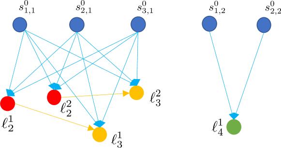
Figure 8: Routing graph ${\mathcal{G}}$ for task (i). $s^{0}_{1,1}$, $s^{0}_{2,1}$ and $s^{0}_{3,1}$ are initial locations of three robots of type 1 and $s^{0}_{1,2}$ and $s^{0}_{2,2}$ are initial locations of two robots of type 2 (see case (a)). Red dots $\ell_{2}^{1}$ and $\ell_{2}^{2}$ correspond to the edge label $\mathcal{\pi}_{{2},{1}}^{2,1}$ of element 3, i.e., edge $(v_{1},v_{2})$ in $X_{P}$; see Fig. 7(b). Yellow dots $\ell_{3}^{1},\ell_{3}^{2}$ correspond to the edge label $\mathcal{\pi}_{{2},{1}}^{3,1}$ of element 4, and green dot $\ell_{4}^{1}$ corresponds to the edge label $\mathcal{\pi}_{{1},{2}}^{4}$ of element 2 (see Appendix (b)). No dots correspond to vertex labels since all vertex labels are either $\top$ or $\bot$. The edges from $\ell_{2}^{1}$ to $\ell_{3}^{1}$ and from $\ell_{2}^{2}$ to $\ell_{3}^{2}$ are due to $3<_{P}4$.

V-A2 Construction of the edge set

The edges in ${\mathcal{G}}$ respect the partial order among subtasks captured by the poset ${P}$. We construct the edge set ${\mathcal{E}}_{\mathcal{G}}$ by following a similar procedure as that used to construct the vertex set ${\mathcal{V}}_{\mathcal{G}}$. Specifically, we iterate over the elements in $X_{P}$. For every subtask $e=(v_{1},v_{2})\in X_{P}$, if $\gamma(v_{1},v_{2})\not=\top$, we first operate on the edge label $\gamma(v_{1},v_{2})=\bigvee_{p\in{\mathcal{P}}}\bigwedge_{q\in{\mathcal{Q}}_{p}}\mathcal{\pi}_{{i},{j}}^{k,\chi}$ starting by iterating over the clauses ${\mathcal{C}}_{p}^{\gamma}\in\mathsf{cls}(\gamma)$, and then over the literals in each clause ${\mathcal{C}}_{p}^{\gamma}$ [lines 2-2, Alg. 2]. Specifically, recall from Appendix V-A1 that the literal $\mathcal{\pi}_{{i},{j}}^{k,\chi}\in\mathsf{lits}^{+}({\mathcal{C}}_{p}^{\gamma})$ corresponds to $i$ vertices in ${\mathcal{V}}_{\mathcal{G}}$ that are associated with region $\ell_{k}$ that should be visited by $i$ robots. In what follows, we identify three types of leaving vertices in ${\mathcal{V}}_{\mathcal{G}}$ from where $i$ robots can depart to reach these $i$ vertices that satisfy literal $\mathcal{\pi}_{{i},{j}}^{k,\chi}$.

(a) Location vertices

The location vertices in ${\mathcal{V}}_{\text{init}}$ associated with robots of type $j$ are leaving vertices. We add an edge from all initial vertices to every vertex associated with literal $\mathcal{\pi}_{{i},{j}}^{k,\chi}$ (see blue edges in Fig. 8). Intuitively, robots depart from initial locations to undertake certain subtasks. These edges are associated with a weight $T^{*}$ that is equal to the shortest travel time from the initial location to region $\ell_{k}$ and another weight $d$ that is equal to the smallest traveling cost between the initial location and $\ell_{k}$, which will be used in the MILP problem in Appendices LABEL:app:scheduling_constraints and LABEL:sec:objective to encode the scheduling constraints and the objective.

(b) Leaving vertices associated with prior subtasks

Let $X^{e}_{<_{P}}$, $X^{e}_{\prec_{P}}$ and $X^{e}_{\|_{P}}$ denote the sets that collect subtasks in $X_{P}$ that are smaller than, covered by, and incomparable to subtask $e$, respectively (see Section II-B). In words, $X^{e}_{<_{P}}$ contains subtasks in $X_{P}$ that should be completed prior to $e$, $X^{e}_{\prec_{P}}\subseteq X^{e}_{<_{P}}$ contains subtasks in $X^{e}_{<_{P}}$ that can be completed right before $e$, and $X^{e}_{\|_{P}}$ contains subtasks independent from $e$. To find leaving vertices, we iterate over $S_{1}^{e}=X^{e}_{<_{P}}\cup X^{e}_{\|_{P}}$ that includes all subtasks that can be completed prior to $e$, respecting the partial order between subtasks. Given a subtask $e^{\prime}=(v^{\prime}_{1},v^{\prime}_{2})\in S_{1}^{e}$, if its edge label $\gamma^{\prime}(v^{\prime}_{1},v^{\prime}_{2})\not=\top$, we iterate over all clauses in $\gamma^{\prime}$ and then over all literals in each clause. Specially, given a clause ${\mathcal{C}}^{\gamma^{\prime}}_{p^{\prime}}\in\mathsf{cls}(\gamma^{\prime})$, for any literal $\mathcal{\pi}_{{i^{\prime}},{j^{\prime}}}^{k^{\prime},\chi^{\prime}}\in\mathsf{lits}^{+}({\mathcal{C}}^{\gamma^{\prime}}_{p^{\prime}})$, if $j^{\prime}=j$, then literal vertices in ${\mathcal{V}}_{\mathcal{G}}$ associated with this literal are leaving vertices. If further $i^{\prime}=i$, we randomly create $i$ one-to-one edges starting from these $i$ vertices and ending at the $i$ vertices associated with $\mathcal{\pi}_{{i},{j}}^{k,\chi}$ (see the orange edges in Fig. 8). Because there are exactly $i$ robots of type $j$, it suffices to build $i$ one-to-one edges. Furthermore, if $\chi=\chi^{\prime}\neq 0$, then literals $\mathcal{\pi}_{{i},{j}}^{k,\chi}$ and $\mathcal{\pi}_{{i^{\prime}},{j^{\prime}}}^{k^{\prime},\chi^{\prime}}$ must have the same number of vertices. Building $i$ one-to-one edges can guarantee that the same $i$ robots of type $j$ satisfy these two literals. Otherwise, if $i^{\prime}\neq i$, we add $i\times i^{\prime}$ edges to ${\mathcal{E}}_{\mathcal{G}}$ by creating an edge from any vertex associated with $\mathcal{\pi}_{{i^{\prime}},{j^{\prime}}}^{k^{\prime},\chi^{\prime}}$ to any vertex of $\mathcal{\pi}_{{i},{j}}^{k,\chi}$. Finally, since each region may span multiple cells, the weights $T^{*}$ and $d$ of these edges are set as the shortest travel time and lowest traveling cost from $\ell_{k^{\prime}}$ to $\ell_{k}$. After creating edges associated with the edge label $\gamma^{\prime}(v^{\prime}_{1},v^{\prime}_{2})$ of $e^{\prime}$, we identify leaving vertices among literal vertices in ${\mathcal{V}}_{\mathcal{G}}$ associated with the starting vertex label $\gamma(v^{\prime}_{1})$ of $e^{\prime}$ and build edges in the same manner.

(c) Leaving vertices associated with $\gamma(v_{1})$ of $e$

When the iteration over $S_{1}^{e}$ is completed, we identify leaving vertices among literal vertices associated with the starting vertex label $\gamma(v_{1})$ of the current subtask $e$ by following the procedure in Appendix (b) for the prior subtasks. This is because $\gamma(v_{1})$ becomes true before $\gamma(v_{1},v_{2})$.

So far we have constructed three types of leaving vertices corresponding to the literal $\mathcal{\pi}_{{i},{j}}^{k,\chi}$ in $\mathsf{lits}^{+}({\mathcal{C}}_{p}^{\gamma})$ of the edge label $\gamma(v_{1},v_{2})$ [lines 2-2, Alg. 2]. We continue constructing leaving vertices for all other literals in $\mathsf{lits}^{+}({\mathcal{C}}_{p}^{\gamma})$ [line 2, Alg. 2] and clauses in $\mathsf{cls}(\gamma)$ [line 2, Alg. 2]. After constructing all edges pointing to vertices associated with literals in the edge label $\gamma(v_{1},v_{2})$ of the current subtask $e$ [line 2, Alg. 2], we construct edges pointing to vertices associated with literals in the starting vertex label $\gamma(v_{1})$, by identifying leaving vertices among location vertices and literal vertices associated with prior subtasks. Specifically, let $S_{2}^{e}=X_{\prec_{P}}^{e}\cup X_{\|_{P}}^{e}$ be the set that collects all subtasks that can occur immediately prior to subtask $e$. The satisfaction of edge labels of subtasks in $S_{2}^{e}$ can directly lead to the starting vertex $v_{1}$ of $e$. We consider the following cases.

(1) $S_{2}^{e}=\emptyset$: In this case, no subtask can be completed before subtask $e$, i.e., the subtask $e$ should be the first one among all in $X_{P}$ to be completed. Thus, $v_{1}$ is identical to the initial vertex $v_{0}$. In this case, we only identify location vertices as leaving vertices, as in Appendix (a) [lines 2, Alg. 2].

(2) $S_{2}^{e}\neq\emptyset$: We identify leaving vertices associated with prior subtasks in $S_{2}^{e}$. Given a subtask $e^{\prime}=(v_{1}^{\prime},v_{2}^{\prime})\in S^{e}_{2}$, we find all clauses ${\mathcal{C}}_{p^{\prime}}^{\gamma^{\prime}}\in\mathsf{cls}(\gamma^{\prime})$ in the edge label $\gamma^{\prime}$ of $e^{\prime}$ such that, for the considered clause ${\mathcal{C}}_{p}^{\gamma}\in\mathsf{cls}(\gamma)$ in the starting vertex label of subtask $e$, its corresponding clause $({\mathcal{C}}_{p}^{\gamma})_{\phi}$ in ${\mathcal{A}}_{\phi}$ is the subformula of their corresponding clauses $({\mathcal{C}}_{p^{\prime}}^{\gamma^{\prime}})_{\phi}$ in ${\mathcal{A}}_{\phi}$. Next, for each literal $\mathcal{\pi}_{{i},{j}}^{k,\chi}\in\mathsf{lits}^{+}({\mathcal{C}}_{p}^{\gamma})$ we create $i$ one-to-one edges, starting from those $i$ vertices associated with the counterpart of literal $\mathcal{\pi}_{{i},{j}}^{k,\chi}$ in the found clause ${\mathcal{C}}_{p^{\prime}}^{\gamma^{\prime}}\in\mathsf{cls}(\gamma^{\prime})$ and ending at the $i$ vertices associated with $\mathcal{\pi}_{{i},{j}}^{k,\chi}$ [lines 2, Alg. 2]. We create such one-to-one edges based on condition (d) in Definition III.8 and condition (b) in Definition III.10. That is, the edge label strongly implies its end vertex label, the satisfied clause in the edge label implies the satisfied clause in the end vertex label, and the fleet of robots satisfying the clause in the vertex label belongs to the fleet of robots satisfying the clause in the incoming edge label. This is also the reason why we consider prior subtasks in $S_{2}^{e}$ rather than $S_{1}^{e}$ as in Appendix (b).

(3) $X_{\prec_{P}}^{e}=\emptyset$ and $X_{\|_{P}}^{e}\neq\emptyset$: In this case, the subtask $e$ can be the first one among all to be completed. If so, its starting vertex label $\gamma(v_{1})$ should be satisfied at the beginning. However, robots cannot depart from leaving vertices that are literal vertices (see case (c) in Appendix (c)), because these edges are enabled after subtask $e$. Therefore, for the vertex label $\gamma(v_{1})$, we additionally identify leaving vertices pointing to initial robot locations, as in Appendix (a) [lines 2, Alg. 2]. Note that, if $X_{\prec_{P}}^{e}\neq\emptyset$, there are no leaving vertices associated with initial locations since there exists a subtask that should be completed before $e$ and, therefore, subtask $e$ can not be the first one. When the iteration over all subtasks in $X_{P}$ is over, we finish the construction of the edge set ${\mathcal{E}}_{\mathcal{G}}$ [line 2, Alg. 2].

Remark V.1 (Relaxation of strong implication in condition (d) in Definition III.8)

Condition (d) in Definition III.8 requires that an edge label strongly implies its end vertex label. This condition ensures both that the satisfaction of an edge label leads to the satisfaction of its end vertex label and that when constructing the routing graph ${\mathcal{G}}$, robots satisfying the positive subformula in an end vertex label belong to robots satisfying the corresponding edge label (see step (c) in Appendix (c)). This condition can be relaxed to requiring that an edge label implies its end vertex label (see Definition III.7), which can still ensure that the satisfaction of an edge label implies the satisfaction of its end vertex label, so that the previous instance of GMRPP still activates the immediately following instance of GMRPP. The only change needed in this case is in the pre-processing steps in Section III-D2 where we need to remove all clauses in an end vertex label that are not a subformula of clauses in the corresponding edge label. This way, the edge label strongly implies the remaining clauses in its end vertex label.

V-B Construction of the robot prefix plans

Given the routing graph constructed in Section V-A, the proposed MILP contains five types of constraints including routing constraints, scheduling constraints, logical constraints, temporal constraints, and transition constraints; see Appendix LABEL:app:milpformulation. The feasibility of the MILP and the properties of the resulting solutions are analyzed in Lemmas LABEL:prop:feasibility and LABEL:prop:run. Given the solution to the MILP, we first define a time axis that includes the sorted completion times of all subtasks in $X_{P}$. This time axis produces a linear extension of the poset $P$ and the plan generated by this linear extension satisfies the vertex and edge labels in a given simple path in ${\mathcal{A}}_{\textup{subtask}}^{-}$. Next, we extract a time-stamped task allocation plan, augmented with completion time of each subtask, for each robot that can be used to generate low-level paths satisfying the specification $\phi$.

V-B1 Time axis

The progress made in ${\mathcal{A}}_{\textup{subtask}}^{-}$ is directly linked to the satisfaction of edge labels which, by condition (d) in Definition III.8, implies the satisfaction of their end vertex labels, excluding $v_{\textup{accept}}$. Therefore, we collect the completion times of all subtasks in $X_{P}$ (the time when edges are enabled) and sort them in an ascending order to form a single increasing time axis, denoted by $\vec{t}$. We note that there are no identical time instants in the time axis since, by construction, the solution to the MILP is a simple path in ${\mathcal{A}}_{\textup{subtask}}^{-}$ and subtasks in any simple path are completed at different times.

V-B2 High-level robot plans

Next we extract a high-level plan for each robot, which is a sequence of waypoints that the robots need to visit to complete the subtasks in $X_{P}$ along with the time instants of these visits. Specifically, for each robot $[r,j]$, let $p_{r,j}$ denote its corresponding high-level plan and let $t_{r,j}$ denote its timeline. Consider also a vertex $v^{*}_{0}\in{\mathcal{V}}_{\text{init}}$ in the routing graph ${\mathcal{G}}$ that is associated with the initial location of robot $[r,j]$ and let $v^{*}_{1}$ be the vertex that robot $r$ traverses to. Note that robot $r$ can only travel along one outgoing edge of $v_{0}^{*}$. Note also that each vertex in the routing graph ${\mathcal{G}}$ is associated with a label captured in the mapping ${\mathcal{M}}_{\mathsf{lits}}^{{\mathcal{V}}}$. If the label associated with $v_{1}^{*}$ is a vertex label, then we proceed to the next vertex $v_{2}^{*}$ that robot $r$ reaches from $v_{1}^{*}$, until a vertex $v^{*}\in{\mathcal{V}}_{\mathcal{G}}$ associated with an edge label is found. Then, the region associated with this vertex $v^{*}$, captured by the mapping ${\mathcal{M}}^{\mathcal{V}}_{{\mathcal{L}}}(v^{*})$, constitutes the first waypoint robot $r$ needs to visit to complete a subtask. We add this region ${\mathcal{M}}^{\mathcal{V}}_{{\mathcal{L}}}(v^{*})$ to the plan $p_{r,j}$. Next, the corresponding visit time indicates the completion time of the associated subtask that is captured by the mapping ${\mathcal{M}}_{e}^{{\mathcal{V}}}(v^{*})$. We add this time instance to timeline $t_{r,j}$. Since each time instant on the time axis $\vec{t}$ corresponds to the completion of one subtask, this visit time in $t_{r,j}$ corresponds to the time instant on $\vec{t}$ that the subtask ${\mathcal{M}}_{e}^{\mathcal{V}}(v^{*})$ is completed. Continuing this process, we can construct for robot $[r,j]$ a sequence of waypoints and the corresponding timeline whose time instants appear on the time axis $\vec{t}$. Given this high-level plan $\{p_{r,j}\}$, we can design low-level executable paths that reconsider the negative literals that were originally removed from the NBA ${\mathcal{A}}_{\textup{relax}}$.

Example 1

continued (Time-stamped task allocation plan) After solving the MILP for the workspace in Fig. 1, the high-level plans and the associated timelines for robots are as follows: $p_{2,1}=p_{3,1}=\{\ell_{2},\ell_{3}\},t_{2,1}=t_{3,1}=\{6,16\},p_{2,2}=\{\ell_{4}\}$, $t_{2,2}=\{10\}$. That is, robots $[2,1]$ and $[3,1]$ visit the office building $\ell_{2}$ at time instant 6, then robot $[2,2]$ visits the control room $\ell_{4}$ at time instant 10, and finally robots $[2,1]$ and $[3,1]$ visit the delivery site $\ell_{3}$ at time instant 16. The remaining robots remain idle. Observe that the lengths of the plans differ since every robot may undertake different number of subtasks. The induced simple path in ${\mathcal{A}}_{\textup{subtask}}^{-}$ in Fig. 7(a) is $v_{\textup{init}},v_{1},v_{2},v_{3},v_{6}$. The associated time axis is $\vec{t}=\{0,6,10,16\}$, one time instant per subtask. In words, the subtask $(v_{\textup{init}},v_{1})$ is completed at time instant 0 and the subtask $(v_{1},v_{2})$ is completed at time instant 6, which corresponds to the event that robots $[2,1]$ and $[3,1]$ visit the office building $\ell_{2}$.

V-C Design of low-level prefix paths

In this section we discuss the correction stage that re-introduces the negative literals to the NBA and corrects the high-level plans designed in Section V-B (if needed) so that they satisfy the specification $\phi$. To this end, we first find the simple path in the NBA ${\mathcal{A}}_{\textup{subtask}}^{-}$ connecting $v_{0}$ and $v_{\textup{accept}}$ using the time axis and the time-stamped task allocation plan. To satisfy the specification $\phi$, for every subtask in the simple path, we formulate a generalized multi-robot path planning (GMRPP) problem. Each GMRPP is essentially a generalization of the multi-robot point-to-point navigation problem, whose goal is to determine a collection of executable paths that allow the robots to complete the current subtask (by enabling the edge label at the end while respecting the starting vertex en route) and automatically activate the next subtask, since the satisfaction of the edge label leads to the satisfaction of the starting vertex of the next subtask. The details can be found in Appendix LABEL:sec:solution2mrta, that also discusses different implementations of the proposed GMRPP (see Appendix LABEL:sec:extension_gmrpp) that depend on whether all or a subset of robots are allowed to move during the execution of the current subtask, since not all robots are responsible for the completion of this subtask, and whether the completion times of subtasks are disjoint or partially overlapping. Finally, the feasibility of the proposed GMRPP is analyzed Lemma LABEL:prop:valid in Appendix LABEL:app:correctness.

V-D Obtaining the best prefix-suffix path

After obtaining the prefix path corresponding to a poset $P\in\{P_{\text{pre}}\}$ for the given pair $v_{0}$ and $v_{\textup{accept}}$, next we find the suffix path around $v_{\textup{accept}}$. For this, we can follow a similar process as this described in Sections V-A$\sim$V-C to find the prefix path for poset $P\in\{P_{\text{pre}}\}$, with the difference that now we treat the accepting vertex $v_{\textup{accept}}$ as both the initial vertex $v_{0}$ and the accepting vertex $v_{\textup{accept}}$. This is because the suffix path is essentially a loop, i.e., the final locations in the suffix path are identical to the initial locations in the suffix path, which are also the final locations in the prefix path; see Appendix LABEL:sec:suf for more details.

Specifically, given the pair $v_{0}$ and $v_{\textup{accept}}$, we solve one MILP for each poset $P^{\prime}\in\{P_{\text{suf}}\}$ to obtain a corresponding suffix path; these MILPs can be infeasible if there are no feasible paths that induce simple paths corresponding to the poset $P^{\prime}$. Then, among all suffix paths for all posets $P^{\prime}\in\{P_{\text{suf}}\}$ we select the one with the lowest cost. This best suffix path corresponds to the prefix path generated from a poset $P\in\{P_{\text{pre}}\}$ for the given pair $v_{0}$ and $v_{\textup{accept}}$. Combining this suffix path with the corresponding prefix path we obtain the best total path associated with the poset $P$ for the given pair $v_{0}$ and $v_{\textup{accept}}$. Then, using cost function (2), we select the best total path over all posets in $\{P_{\text{pre}}\}$ for the given pair $v_{0}$ and $v_{\textup{accept}}$. Finally, by iterating over all pairs of initial and accepting vertices with finite total length, we can obtain the best total path. We highlight that our method can terminate anytime once a feasible path is found, but running the algorithm longer can lead to more optimal feasible paths. Note also that by iterating over the pairs $v_{0}$ and $v_{\textup{accept}}$ and the corresponding posets in the ascending order discussed in Section IV-C, it is more likely that the first solutions we obtain have low cost since they involve fewer subtasks that need to be accomplished. This observation is also validated numerically in Section VII.

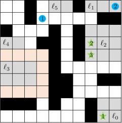
(a) $t=6$

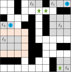
(b) $t=10$

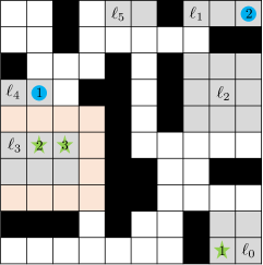
(c) $t=18$

Figure 9: Key frames demonstrating the execution of low-level paths that satisfy task (i). The initial configuration is shown in Fig. 1. Fig. 9(a) shows that at time instant 6, robots $[2,1]$ and $[3,1]$ reach the office building $\ell_{2}$, while robot $[1,2]$ is on the way to the control room $\ell_{4}$. Fig. 9(b) shows at time instant 10, robot $[1,2]$ reaches the control room $\ell_{4}$ while robots $[2,1]$ and $[3,1]$ head towards the delivery site $\ell_{3}$. Finally, they reach $\ell_{3}$ in Fig. 9(c) at time instant 18. Robots $[1,1]$ and $[2,2]$ remain idle throughout the process.

Example 1

continued (Low-level paths) When generating low-level paths for task (i), we also consider collision avoidance. Fig. 9 shows an array of three key frames where different subtasks are completed. Observe that task (i) is completed at time 15, longer than 12 given by the time-stamped task allocation plan since the high-level plan uses the shortest travel time between regions and does not consider collision avoidance.

VI Theoretical Analysis

In this section, we analyze the completeness and soundness of our method. First we show that, with mild assumptions, our method is complete for LTL${}^{0}$ specifications.

Theorem VI.1 (Completeness)

Consider a discrete workspace satisfying Assumption III.5, a team of $n$ robots of $m$ types and a valid specification $\phi\in\textit{LTL}^{0}$. Assume also that there exists a path $\tau=\tau^{\textup{pre}}[\tau^{\textup{suf}}]^{\omega}$ that induces a restricted accepting run $\rho=\rho^{\textup{pre}}[\rho^{\textup{suf}}]^{\omega}=v_{0},\ldots,v_{\textup{prior}},v_{\textup{accept}}$ $[v_{\textup{next}},\ldots,v_{\textup{prior}}^{\prime},v_{\textup{accept}}]^{\omega}$ in the pre-processed NBA ${\mathcal{A}}_{\phi}$ and satisfies Assumption III.11. Then, the proposed synthesis method can find a robot path $\tilde{\tau}=\tilde{\tau}^{\textup{pre}}[\tilde{\tau}^{\textup{suf}}]^{\omega}$ that satisfies the specification $\phi$.

The key idea in the proof of Theorem VI.1 is to first show that feasible paths still exist in ${\mathcal{A}}_{\textup{subtask}}^{-}$ and then use this fact to show feasibility of the MILP and GMRPP problems. The detailed proof can be found in Appendix LABEL:app:correctness. We emphasize that the completeness result in Theorem VI.1 is ensured for LTL${}^{0}$ rather than LTL${}^{\chi}$ formulas. This is because task allocations captured by induced atomic propositions in the prefix part may not lead to feasible allocations in the suffix part. However, when the LTL${}^{\chi}$ specification can be satisfied by finite-length paths, such as co-safe LTL [kupferman2001model] or LTL${}_{f}$ [de2013linear], then our method is complete also for LTL${}^{\chi}$ specifications; This is shown in Proposition LABEL:thm:prefix in Appendix LABEL:app:completeness as part of the proof of Theorem VI.1.

Remark VI.2

We note that the path $\tilde{\tau}$ constructed by our approach may not satisfy Assumption III.11 that requires that robots close their suffix loops at the same time the NBA ${\mathcal{A}}_{\phi}$ transitions to $v_{\textup{accept}}$. However, in our method, when the NBA ${\mathcal{A}}_{\phi}$ transitions to $v_{\textup{accept}}$, only those robots involved in the completion of the last subtask in the prefix part return to regions corresponding to their initial locations. Thereafter, trajectories are closed.

The following statement shows the soundness of our method, which is a direct consequence of Theorem VI.1.

Corollary VI.3 (Soundness)

Consider a discrete workspace, a team of $n$ robots of $m$ types and a valid specification $\phi\in\textit{LTL}^{\chi}$. Then, the path returned by the GMRPP satisfies the specification $\phi$. Also, the specific implementation of the GMRPP is not important.

VII Numerical Experiments

In this section we present three case studies, implemented in Python 3.6.3 on a computer with 2.3 GHz Intel Core i5 and 8G RAM, that illustrate the correctness and scalability of our method. The MILP is solved using Gurobi [gurobi] with big-M $M_{\text{max}}=10^{5}$. First, we compare with the optimal solution to examine the suboptimality of our proposed method when the NBA can be captured by one poset (thus, only one solution). Second, we generate multiple solutions for specifications with multiple posets, and compare the cost of the first solution corresponding to the widest poset to that of the subsequent solutions. We observe that the quality of the first solution obtained for the widest poset is generally very good. Finally, we compare our method to the approach proposed in [sahin2019multi] for large workspaces and numbers of robots and show that our method outperforms the approach in [sahin2019multi] in terms of optimality and scalability. We emphasize that the sets of restricted accepting runs of all specifications $\phi_{1}-\phi_{10}$ considered in the following simulations, are nonempty, which shows that this assumption is not restrictive in practice.

VII-A Case study I: Suboptimality

In this case study, we examine the quality of the paths constructed for the two tasks in the Example 1. Observe that in Fig. 7(a), a unique poset corresponds to the sub-NBA ${\mathcal{A}}_{\textup{subtask}}^{-}$ for task (i). A similar observation can be made for the sub-NBA ${\mathcal{A}}_{\textup{subtask}}^{-}$ in Fig. 5(b) for task (ii). In the workspace shown in Fig. 9, we randomly generate the initial locations of all robots inside label-free cells. To measure the suboptmality of our solution in terms of path length (travelled distance), we use brute-force search to find the optimal cost.

TABLE I: Statistics on the optimal cost and solutions

task	$J^{*}$	NoCol$+$Seq		Col$+$Sim
		cost	horizon	cost	horizon
(i)	36.0$\pm$5.1	36.4$\pm$5.3 (35)	23.9$\pm$4.1	38.8$\pm$5.5	19.6$\pm$2.8
(ii)	25.4$\pm$2.8	28.6$\pm$3.1 (8)	29.2$\pm$2.9	28.6$\pm$3.1	29.2$\pm$2.9

Case Study I: Column “NoCol$+$Seq” represents the case where collision avoidance is ignored and robots move sequentially, and column “Col$+$Sim” incorporates collision avoidance and simultaneous execution. The notation $J^{*}$ denotes the optimal cost without considering collision avoidance. The number of trials out of 50 trials where the cost cost is equivalent to the optimal cost $J^{*}$ are shown inside the parentheses.