[table]capposition=top

A NEW VOLATILITY MODEL: GQARCH-ITÔ MODEL

Volatility asymmetry is a hot topic in high-frequency financial market. In this paper, we propose a new econometric model, which could describe volatility asymmetry based on high-frequency historical data and low-frequency historical data. After providing the quasi-maximum likelihood estimators for the parameters, we establish their asymptotic properties. We also conduct a series of simulation studies to check the finite sample performance and volatility forecasting performance of the proposed methodologies. And an empirical application is demonstrated that the new model has stronger volatility prediction power than GARCH-Itô model in the literature.

Keywords: Volatility asymmetry; Low-frequency historical data; High-frequency historical data; Quasi-maximum likelihood estimators; Volatility prediction power.

MOS subject classification: 62M10, 62M20, 62F12

INTRODUCTION

Volatility measures plays a crucial role in modern financial markets. The wide information source of modeling the volatility is the historical data of the security, which can be further divided into low-frequency data and high-frequency data. High-frequency data and Low-frequency data are two different time scale in financial market. High-frequency data are observed at intra-day for financial assets, while low-frequency data are referred for financial assets at daily or longer time horizons. There are many important models such as Generalized autoregressive conditional heteroskedasticity (GARCH) models (Bollerslev, 1986) used in volatility analysis of low-frequency data. The standard GARCH models describe the squared daily log returns as the conditional volatilities. On the other hand, there are also several well-performing realized volatility estimators, for example, two-time scale realized volatility(TSRV) (Zhang et al., 2005), multi-scale realized volatility(MSRV) (Zhang, 2006), kernel realized volatility(KRV) (Barndorff-Nielsen et al., 2009), pre-averaging realized volatility(PRV) (Jacod et al., 2009) and quasi-maximum likelihood estimator(QMLE) (Xiu, 2010). However, these models were developed for high-frequency data and low-frequency data quite independently. In fact, high-frequency data and low-frequency data must be inter-related at different time scales, due to just these different time scales. Fortunately, there are some attempts to bridge the gap between high-frequency data and low-frequency data. Wang (2002) studies the statistical relationship between the GARCH and diffusion model. Hansen et al. (2012) studies volatilities analysis by combining the realized GARCH model and the high-frequency volatility model. Kim and Wang (2016) proposed GARCH-It$\widehat{o}$ model for merged low-frequency data and high-frequency data.

GARCH-It$\widehat{o}$ model is a unified model for both high-frequency data and low-frequency data, which is a continuous-time It$\widehat{o}$ process at high-frequency data points, and a GARCH model at integer time points. The parameters estimators based on GARCH-It$\widehat{o}$ model have better performances than the estimators using only low-frequency data by asymptotic theory and simulation study.

However, GARCH-It$\widehat{o}$ model has not introduced the volatility asymmetry. Volatility asymmetry is an important phenomenon in financial market. There are two explanation for volatility asymmetry: leverage effect and volatility feedback effect. Black (1976) and Christie (1982) first gave the description of leverage effect: when the asset prices is declining, the companies leverage (dept-to-equity ratio)become larger, so the stock becomes riskier since its volatility is increasing. Therefore, leverage effect implies a negative correlation structure between the analysed asset return and its volatility changes. On the other hand, French et al. (1987) proposed the volatility feedback effect: if volatility is priced, and anticipated increase in volatility would raise the required rate of return, in turn necessitating an immediate stock-price decline to allow for higher future returns.

In recent years, many scholars have studied volatility asymmetry based high-frequency financial data. Bouchaud et al. (2001) proposed the peak effect at the instantaneous correlation between return and volatility over fairly small time intervals. By an application of high-frequency five-minute S&P 500 futures, Bollerslev, Litvinova and Tauchen (2006) found that there exists significantly negative correlation for several days between the absolute high-frequency returns and the current and past returns, and low correlations between the volatility and lagged return. Bollerslev et al. (2009) obtained a highly accurate discrete-time daily stochastic volatility model that distinguishes between the jump and continuous-time components of price movements. Wang and Mykland (2014) proposed the new nonparametric estimators of leverage effect based on the stochastic volatility model. Kalnina and Xiu (2017) provided the integrated leverage effect estimator, and gave its the statistical properties. Curato (2019) presented the non-parameter estimator of leverage effect via Fourier transformation. Bibinger et al. (2019) explored the non-continuous leverage effect in 320 NASDAQ corporations.

As we all known, GARCH-It$\widehat{o}$ model have better statistical performance than other current volatility models. It is natural to extend GARCH-It$\widehat{o}$ model to a unified model describing the volatility asymmetry. Many empirical analysis told us that the complex models would sometimes perform worse properties, and time-consuming, therefore, we try to look for a volatility model with minor modifications for GARCH-It$\widehat{o}$ model. Fortunately, Sentana (1995) proposed Quadratic ARCH(QARCH) and Generalized QARCH(GQARCH) model, which can be integrated in economic models and provides a very simple way of calibrating and testing for dynamic asymmetries for some financial times. Inspired by this, we expand GARCH-It$\widehat{o}$ model so that features of financial data at both frequencies can be better captured as follows. First, volatility asymmetry that are described in empirical studies are allowed. Second, we explore that volatility forecasting performances for $\frac{1}{j},j=1,2,3,4,5,6$ of daily volatility. We name the proposed model as the GQARH-It$\widehat{o}$ model. The key feature of the proposed model is that its conditional volatility has integrated volatility and asymmetry as innovations.

The paper is organized as follows. Section 2 introduces the GQARCH-It$\widehat{o}$ model. Section 3 introduces quasi-likelihood estimation methods and investigates their asymptotic behaviors. Section 4 conducts the simulation studies to check the finite sample performance and different volatility forecasting performances for the proposed model. Section 5 carries out an empirical analysis with CRPS total market index to demonstrate the advantage of the proposed model in volatility forecasting. We collect the proofs in the Appendix.

GQARCH-ITÔ MODEL

2.1 GQARCH(1,1) model at discrete-time

In order to capture dynamic asymmetric that GARCH model rules out, Sentana (1995) proposed GQARCH model, which allows an asymmetric effect on the conditional variance, and GQARCH(1,1) model structure is as follows,

$$X_{t}-X_{t-1}= \mu+\xi_{t},$$

$$\xi_{t}= \sigma_{t}\varepsilon_{t},$$

$$\sigma_{t}^{2}= \kappa+\sigma_{t-1}^{2}+\varphi\xi_{t-1}^{2}+\phi\xi_{t-1},$$

where $X_{t}$ is the ture log price at integrated time $t=1,2,\cdots,n$, $\sigma_{t}$ is volatility, $\varepsilon_{t}$ is i.i.d varibles and random errors $\xi_{t}$ satisfy $E\left[\xi_{t}\bigg{|}\mathcal{F}_{t-1}^{LF}\right]=0$ a.s., $\mathcal{F}_{t}^{LF}=\sigma(X_{t},X_{t-1},\cdots)$. Therefore, their conditional variances obey,

$$E\left[\xi_{t}^{2}\bigg{|}\mathcal{F}_{t-1}^{LF}\right]=\kappa+E\left[\xi_{t-1}^{2}\bigg{|}\mathcal{F}_{t-2}^{LF}\right]+\varphi\xi_{t-1}^{2}+\phi\xi_{t-1}.$$ (2.1)

Equation (2.1) is different from the conditional variances of GARCH model, this is because GQARCH model incorporate the term $\xi_{t-1}$.

2.2 GQARCH-Itô model

In this subsection, we try to provide a volatility model that describes the volatility asymmetry by embedding a standard GQARCH(1, 1) model into an Itô process with an instantaneous volatility as follows. Noted that $\mathbb{R}_{+}=[0,\infty]$ and $\mathbb{N}$ is the set of all non-negative integers.

Definition 1.

We call a log security price $X_{t}$, $t\in[0,+\infty)$, to follow a unified GQARCH-Itô model, if it satisfies

$$\begin{array}[]{rl}dX_{t}=&\mu dt+\sigma_{t}dB_{t},\\ \sigma_{t}^{2}=&\sigma_{[t]}^{2}+(t-[t])\left\{\omega+(\gamma-1)\sigma_{[t]}^{2}\right\}+\beta\left(\displaystyle\int_{[t]}^{t}\sigma_{s}dB_{s}\right)^{2}+\alpha\displaystyle\int_{[t]}^{t}\sigma_{s}dB_{s},\end{array}$$ (2.2)

where $\mu$ is a drift, $B_{t}$ is a standard Brownian motion with respect to a filtration $\mathcal{F}_{t}$, $\sigma_{t}^{2}$ is the instantaneous volatility process adapted to $\mathcal{F}_{t}$, $[t]$ denotes the integer part of $t$, $\theta=\left(\omega,\gamma,\beta,\alpha\right)$.

According to Definition 1, GQARCH-Itô model is a continuous Itô process defined at all times $t\in\mathbb{R}_{+}$. When it is restricted to integer times $t\in\mathbb{N}$, the conditional variance of daily return $X_{t}-X_{t-1}$ follows a GQARCH(1,1) structure,

$$E\left[Z_{t}^{2}\bigg{|}\mathcal{F}_{t-1}^{LF}\right]= \omega_{1}^{g}+\gamma E\left[Z_{t-1}^{2}\bigg{|}\mathcal{F}_{t-2}^{LF}\right]+\beta_{1}^{g}Z_{t-1}^{2}+\alpha_{1}^{g}Z_{t-1},$$

$$Z_{t}= \displaystyle\int_{t-1}^{t}\sigma_{s}dB_{s},t\in\mathbb{N},$$

where $\mathcal{F}_{t}^{LF}=\sigma(X_{t},X_{t-1},\cdots)$, $\omega_{1}^{g}=\beta^{-1}\left(e^{\beta}-1\right)\omega,\beta_{1}^{g}=\beta^{-1}(\gamma-1)\left(e^{\beta}-1-\beta\right)+e^{\beta}-1,$ and $\alpha_{1}^{g}=\alpha\left(\beta^{-2}(\gamma-1)\left(e^{\beta}-1-\beta\right)+\beta^{-1}\left(e^{\beta}-1\right)\right)$ (see: Proposition 1). Therefore, our proposed GQARCH-Itô model could capture the asymmetries based on low-frequency historical data and high-frequency historical data. The asymmetry explanation is the same as GQARCH model in Sentana (1995)’ paper.

2.3 Integrated volatility for GQARCH-Itô model

In general, the trade period is about six and half hours in financial market, the financial sectors often focus on the several hours volatility prediction rather than daily volatility. Therefore, we would study the $\frac{1}{j},j=1,2,3,4,5,6$ of daily volatility obtained from the GQARCH-Itô model over consecutive integers.

Proposition 1.

(a) Under GQARCH-Itô model, we have, for any $k,n\in\mathbb{N}$ and $0<\beta<1$,

$$R(k)\equiv \int_{n-\frac{1}{j}}^{n}\frac{(n-t)^{k}}{k!}\sigma_{t}^{2}dt$$

$$= \frac{\omega+(\gamma+j(k+2)-1)\sigma_{n-\frac{1}{j}}^{2}}{(k+2)!}\left(\frac{1}{j}\right)^{k+2}+\beta R(k+1)+2\beta\int_{n-\frac{1}{j}}^{n}\frac{(n-t)^{k+1}}{(k+1)!}\int_{n-\frac{1}{j}}^{t}\sigma_{s}dB_{s}\sigma_{t}dB_{t}$$

$$+ \alpha\int_{n-\frac{1}{j}}^{n}\frac{(n-t)^{k+1}}{(k+1)!}\sigma_{t}dB_{t}.$$

In particular,

$$\int_{n-\frac{1}{j}}^{n}\sigma_{t}^{2}dt$$

$$= \sum_{k=0}^{\infty}\frac{\beta^{k}\left[\omega+(\gamma+j(k+2)-1)\sigma_{n-\frac{1}{j}}^{2}\right]}{(k+2)!}\left(\frac{1}{j}\right)^{k+2}+\sum_{k=0}^{\infty}2\int_{n-\frac{1}{j}}^{n}\frac{\left[\beta(n-t)\right]^{k+1}}{(k+1)!}\int_{n-\frac{1}{j}}^{t}\sigma_{s}dB_{s}\sigma_{t}dB_{t}$$

$$+ \sum_{k=0}^{\infty}\int_{n-\frac{1}{j}}^{n}\frac{\alpha\left(n-t\right)^{k+1}}{(k+1)!}\beta^{k}\sigma_{t}dB_{t}$$

$$= g_{n}(\theta)+D_{n},$$

where

$$g_{n}(\theta)= \omega_{j}^{g}+\frac{\gamma+j-1}{j}g_{n-\frac{1}{j}}(\theta)+\beta_{j}^{g}Z_{n-\frac{1}{j}}^{2}+\alpha_{j}^{g}Z_{n-\frac{1}{j}},$$ (2.3)

the parameters are given as

$$\omega_{j}^{g}= \beta^{-1}\left(e^{\frac{\beta}{j}}-1\right)\frac{\omega}{j},\quad\beta_{j}^{g}=\beta^{-1}(\gamma-1)\left(e^{\frac{\beta}{j}}-1-\frac{\beta}{j}\right)+e^{\frac{\beta}{j}}-1,$$

$$\alpha_{j}^{g}= \alpha\left(\beta^{-2}(\gamma-1)\left(e^{\frac{\beta}{j}}-1-\frac{\beta}{j}\right)+\beta^{-1}\left(e^{\frac{\beta}{j}}-1\right)\right),$$

and

$$D_{n}=2\int_{n-\frac{1}{j}}^{n}\left(e^{(n-t)\beta}-1\right)\int_{n-\frac{1}{j}}^{t}\sigma_{s}dB_{s}\sigma_{t}dB_{t}+\frac{\alpha}{\beta}\int_{n-\frac{1}{j}}^{n}(e^{\left(n-t\right)\beta}-1)\sigma_{t}dB_{t},$$

is a martingale difference.

(b) For any $k,n\in\mathbb{N}$ and $0<\beta<1$, we have

$$E\left[\int_{n-\frac{1}{j}}^{n}\frac{(n-t)^{k}}{k!}\sigma_{t}^{2}dt\bigg{|}\mathcal{F}_{n-1}\right]$$

$$= \frac{\omega+(\gamma+j(k+2)-1)\sigma_{n-\frac{1}{j}}^{2}}{(k+2)!}\left(\frac{1}{j}\right)^{k+2}+\beta E\left[\int_{n-\frac{1}{j}}^{n}\frac{(n-t)^{k+1}}{(k+1)!}\sigma_{t}^{2}dt\bigg{|}\mathcal{F}_{n-1}\right].$$

In particular,

$$E\left[\int_{n-\frac{1}{j}}^{n}\sigma_{t}^{2}dt\bigg{|}\mathcal{F}_{n-1}\right]=g_{n}(\theta).$$

When $j=1$, Proposition 1 denotes the daily volatility $\int_{n-1}^{n}\sigma_{t}^{2}dt$ consist of $g_{n}(\theta)$ and a martingale difference $D_{n}$. Where

$$g_{n}(\theta)= \omega_{1}^{g}+\gamma g_{n-1}(\theta)+\beta_{1}^{g}Z_{n-1}^{2}+\alpha_{1}^{g}Z_{n-1},$$ (2.4)

and

$$D_{n}=2\int_{n-1}^{n}\left(e^{(n-t)\beta}-1\right)\int_{n-1}^{t}\sigma_{s}dB_{s}\sigma_{t}dB_{t}+\frac{\alpha}{\beta}\int_{n-1}^{n}(e^{\left(n-t\right)\beta}-1)\sigma_{t}dB_{t},$$ (2.5)

According to (2.4), $g_{n}(\theta)$ includes the term $\alpha_{1}^{g}Z_{n-1}$, which denotes the volatility asymmetry.

PARAMETER ESTIMATION FOR GQARCH-ITÔ MODEL

3.1 Quasi-maximum likelihood estimation

The underlying log price process is assumed to obey the GQARCH-Itô model as described in Definition 1. Let $n$ be the total number of low-frequency observations and $m_{i}$ be the total number of high-frequency observations duiring the $i$th low-frequency period, for example, the $i$th day. Furthermore, the low-frequency historical data are observed true log prices at integer times, namely $X_{i},i=0,1,2,\cdots,n$, and the high-frequency historical data are observed log prices at time points between integer times, that is, $t_{i,j}$, $j=0,1,\cdots,m_{i}$, denote the high-frequency time points during the $i$-th period satisfying $i-1=t_{i,0}<t_{i,1}<\ldots<t_{i,m_{i}}<t_{i,m_{i}}=t_{i+1,0}=i$. As we all known, the true high-frequency log prices are not observable, and the observed high-frequency log prices are contaminated by the market micro-structure noise. In this regard, we assume that observed high-frequency log prices $Y_{t_{i,j}}$ obey the simple additive noise model,

$$Y_{t_{i,j}}=X_{t_{i,j}}+\epsilon_{t_{i,j}},$$ (3.1)

where $\epsilon_{t_{i,j}}$ is micro-structure noise independent of the process of $X_{t_{i,j}}$, and for each $i$, $\epsilon_{t_{i,j}},j=1,\cdots,m_{i}$, are independent and identically distributed (i.i.d.) with mean zero and variance $a^{2}$.

Similar to Kim and Wang (2016), we propose the quasi-likelihood function $\widetilde{L}_{n,m}^{GH}$ for GQARCH-Itô model as follows,

$$\widetilde{L}_{n,m}^{GH}(\theta)= -\frac{1}{2n}\sum_{i=1}^{n}\left(\log g_{i}(\theta)+\frac{RV_{i}}{g_{i}(\theta)}\right),$$

where $g_{i}(\theta)$ has the structure of (2.4), and the realized volatility $RV_{i}$ is computed using $m_{i}$ high-frequency historical data during the $i$-th period and is treated as an “observation”. $RV_{i}$ could be estimated by two-time scale realized volatility (TSRV) (Zhang et al., 2005), multi-scale realized volatility (MSRV) (Zhang, 2006), kernel realized volatility (KRV) (Barndorff-Nielsen et al., 2009), pre-averaging realized volatility (PRV) (Jacod et al., 2009) and quasi-maximum likelihood estimator (QMLE) (Xiu, 2010) among others.

We maximize the quasi-likelihood function $\widetilde{L}_{n,m}^{GH}(\theta)$ over parameters’ space $\theta$ and denote the maximizer as $\widetilde{\theta}^{GH}$, that is,

$$\widetilde{\theta}^{GH}=\arg\max\limits_{\theta\in\Theta}\widetilde{L}_{n,m}^{GH}(\theta).$$

$\widetilde{\theta}^{GH}=(\omega^{GH},\beta^{GH},\gamma^{GH},\alpha^{GH})$ are the quasi-maximum likelihood estimators of $\theta_{0}=(\omega_{0},\beta_{0},\gamma_{0},\alpha_{0})$.

3.2 Asymptotic theory of estimators

In this subsection, we establish consistency and asymptotic distribution for the proposed estimators $\widetilde{\theta}^{GH}=(\omega^{GH},\beta^{GH},\gamma^{GH},\alpha^{GH})$.

First, we fix some notations. Given a random variable $X$ and $p\geq 1$, let $||X||_{L_{p}}=\{E[|X|^{p}]\}^{1/p}$. For a matrix $A=(A_{i,j})_{i,j=1,\dots,k}$, and a vector $a=(a_{1},\dots,a_{k})$, define $||A||_{\max}=\max_{i,j}|A_{i,j}|$ and $||a||_{\max}=\max_{i}|a_{i}|$. Let $C$ be positive generic constants whose values are free of $\theta$, $n$ and $m_{i}$, and may change from appearance to appearance. Then, we give the following assumptions, under which the asymptotic theory is established.

Assumption 1.

(a) Let

$$\Theta= \{\theta=(\omega_{1},\beta_{1},\gamma,\alpha_{1})~{}|~{}\omega_{l}<\omega_{1}<\omega_{u},~{}\beta_{l}<\beta_{1}<\beta_{u},~{}\gamma_{l}<\gamma<\gamma_{u},~{}\alpha_{l}<\alpha_{1}<\alpha_{u},$$

where $\omega_{l}$, $\omega_{u}$, $\beta_{l}$, $\beta_{u}$, $\gamma_{l}$, $\gamma_{u}$, $\alpha_{l}$, $\alpha_{u}$,are known constants.

(b) $\left\{|D_{i}|~{}|~{}i\in\mathbb{N}\right\}$ is uniformly integrable.

(c) One of the following conditions is satisfied.

(c1) $\frac{E\left[Z_{i}^{4}|\mathcal{F}_{i-1}\right]}{g_{i}^{2}(\theta_{0})}\leq C$ a.s. for any $i\in\mathbb{N}$.

(c2) There exists a positive constant $\delta$ such that $E\left[\left(\frac{Z_{i}^{2}}{g_{i}(\theta_{0})}\right)^{2+\delta}\right]\leq C$ for $i\in\mathbb{N}$.

(d) $(D_{i},Z_{i}^{2})$ is a stationary ergodic process.

(e) Let $m=\sum_{i=1}^{n}m_{i}/n$. We have $C_{1}m\leq m_{i}\leq C_{2}m$, $\sup\limits_{1\leq j\leq m_{i}}|t_{i,j}-t_{i,j-1}|=O(m^{-1})$ and $n^{2}m^{-1}\rightarrow 0$ as $m,n\rightarrow\infty$.

(f) $\sup\limits_{i\in\mathbb{N}}\left\|RV_{i}-\int_{i-1}^{i}\sigma_{t}^{2}dt\right\|_{L_{1+\delta}}\leq C\cdot m^{-1/4}$ for some $\delta>0$.

(g) For any $i\in\mathbb{N}$, $E\left[RV_{i}|\mathcal{F}_{i-1}\right]\leq C\cdot E[\int_{i-1}^{i}\sigma_{t}^{2}dt|\mathcal{F}_{i-1}]+C$ a.s.

Comparing to the Assumption 1 in Kim and Wang (2016), we add one additional Assumption 1(a) on $\alpha_{l}<\alpha<\alpha_{u}$. Among Assumption 1, (a)-(d) are for the low-frequency part of the model, while (e)-(g) are for the high-frequency part of the model. Similar to the explanation in Kim and Wang (2016), these assumptions are also all reasonable in this paper. The following theorem would give the consistency and convergence rate for $\widetilde{\theta}^{GH}$.

Theorem 1.

(a) Under Assumption 1(a), (b), (d), (f)-(g), there is a unique maximizer of $L_{n}^{GH}(\theta)$ and as $m,n\rightarrow\infty$, $\widetilde{\theta}^{GH}\rightarrow\theta_{0}$ in probability, where

$$L_{n}^{GH}(\theta)=-\frac{1}{2n}\sum_{i=1}^{n}\log(g_{i}(\theta))-\frac{1}{2n}\sum_{i=1}^{n}\frac{g_{i}(\theta_{0})}{g_{i}(\theta)}.$$

(b) Under Assumption 1(a)-(d), (f)-(h), we have

$$\left\|\widetilde{\theta}^{GH}-\theta_{0}\right\|_{\max}=O_{p}\left(m^{-1/4}+n^{-1/2}\right).$$

Theorem 1 shows that $\widetilde{\theta}^{GH}$ has the same convergence rate as the parameter estimators in GARCH-Itô model of Kim and Wang (2016). In other words, the asymmetry information has no significant effect on the converge rate of the parameter estimators. The following theorem shows the asymptotic normality of $\widetilde{\theta}^{GH}$.

Theorem 2.

Under Assumption 1, we have as $m,n\rightarrow\infty$,

$$\sqrt{n}(\widetilde{\theta}^{GH}-\theta_{0})\xrightarrow{d}N(0,B^{-1}A^{GH}B^{-1}),$$

where

$$A^{GH}= \frac{1}{4}E\left[\frac{\partial g_{1}(\theta)}{\partial\theta}\frac{\partial g_{1}(\theta)}{\partial\theta^{T}}\bigg{|}_{\theta=\theta_{0}}g_{1}^{-4}(\theta_{0})\right.$$

$$\left.\int_{0}^{1}\left[4(e^{\beta_{0}(1-t)}-1)^{2}(X_{t}-X_{0})^{2}+\frac{4\alpha_{0}}{\beta_{0}}(e^{\beta_{0}(1-t)}-1)^{2}(X_{t}-X_{0})+\frac{\alpha_{0}^{2}}{\beta_{0}^{2}}(e^{\beta_{0}(1-t)}-1)^{2}\right]\sigma_{t}^{2}dt\right],$$

$$B= \frac{1}{2}E\left[\frac{\partial g_{1}(\theta)}{\partial\theta}\frac{\partial g_{1}(\theta)}{\partial\theta^{T}}\bigg{|}_{\theta=\theta_{0}}g_{1}^{-2}(\theta_{0})\right].$$

According to Theorem 2, we could see that $A^{GH}$ represent the influences of volatility asymmetry on the asymptotic variances of the parameter estimators.

SIMULATION STUDY

4.1 Asymptotic Performance

In this section, we generate the log prices $X_{t_{i,j}},~{}t_{i,j}=i-1+j/m,~{}i=1,\cdots,n,~{}j=1,\cdots,m$, from the GQARCH-Itô models with $\theta_{0}=(\omega_{0},\beta_{0},\gamma_{0},\alpha_{0})=(0.2,0.3,0.4,0.1)$. We further set $n=250,m=2160$, and $X_{0}=10$, which implies that $\sigma_{0}^{2}=0.667$. The high-frequency data $Y_{t_{i,j}}$ are obtained through model (3.1) by simulating $\epsilon_{t_{i,j}}$ from $N(0,0.001^{2})$. The multi-scale realized volatility estimator is used to estimate $RV_{i}$. All boxplots of estimators are displayed in Figure 1. We can see clearly that our proposed estimators have good statistical performance and the simulation confirms most of the theoretical findings in Section 3.

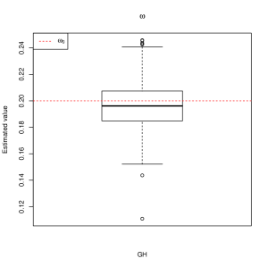
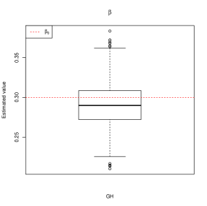
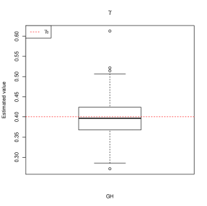
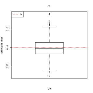
Figure 1: Boxplots of $\widetilde{\theta}^{GH}$ for estimating $\theta_{0}=(\omega_{0},\beta_{0},\gamma_{0},\alpha_{0})$ base on simulated data, where GH represents $\widetilde{\theta}^{GH}$.

4.2 Prediction Performance under different theoretical volatility models

In this subsection, we simulate the sample data from two theoretical volatility models, Heston model and Jump-diffusion model. Under each theoretical volatility model, we simulate high-frequency time interval for 10 seconds, and we report the out-of-sample prediction performances of GQARCH-Itô model for $\frac{1}{j},j=1,2,3,4,5,6$ of daily volatility.

4.2.1 Heston stochastic volatility model

In this Monte Carlo experiment, we use as the data generating process the stochastic volatility model of Heston(1993) for the instantaneous variance

$$\begin{split}dS(t)=&rS(t)dt+\sqrt{V(t)}S(t)dW_{1}(t)\\ dV(t)=&(a-bV(t))dt+\gamma\sqrt{V(t)}dW_{2}(t).\end{split}$$ (4.1)

parameter $a,b,\gamma$ is positive, $W_{1}(t),W_{2}(t)$ are Brownian motions, and $\rho$ is the correlation coefficient between $W_{1}(t)$ and $W_{2}(t)$. We set parameters $a_{0}=0.01$, $b_{0}=0.001$, $\gamma_{0}=0.075$, $\rho_{0}=-0.8$, and $r_{0}=0.02$. We further set $n=101,S_{0}=50,V_{0}=0.05$. We simulated the high-frequency data with 10 seconds interval, and $\frac{1}{2}$, $\frac{1}{3}$, $\frac{1}{4}$, $\frac{1}{5}$ and $\frac{1}{6}$ of daily volatility forecasting results are also presented in the studies. All simulation is based 1000 repetitions, and the first 100 days are used for in-sample, and the 101th day is saved for the out-of-sample forecast of daily volatility. We define the following four criteria to evaluate the forecasting error, which are mean absolute error (MAE), mean square error (MSE), adjusted mean absolute percentage error (AMAPE) and logarithmic loss (LL),

$$MAE=\frac{1}{N}\sum_{i=1}^{N}|RV_{i}-F_{i}|,\quad MSE=\frac{1}{N}\sum_{i=1}^{N}(RV_{i}-F_{i})^{2},$$

$$AMAPE=\frac{1}{N}\sum_{i=1}^{N}\left|\frac{F_{i}-RV_{i}}{F_{i}+RV_{i}}\right|,\quad LL=\frac{1}{N}\sum_{i=1}^{N}(\log(F_{i})-\log(RV_{i}))^{2},$$

where the realized volatility $RV_{i}$ is considered as the best estimation of the real integrated volatility in day $i$, $F_{i}$ is the volatility prediction in day $i$. All results are presented in Table 1.

According to Table 1, we may get some interesting findings. First, our proposed model could predict the $\frac{1}{2}$, $\frac{1}{3}$, $\frac{1}{4}$, $\frac{1}{5}$ and $\frac{1}{6}$ of daily volatility. This is very important in financial market since that a large number of securities’ practitioners would like to know the volatility performances for next half day, one-third days, one-fourth days, one-fifth days and even one-sixth days rather than future daily volatility. Second, the $\frac{1}{2}$, $\frac{1}{3}$, $\frac{1}{4}$, $\frac{1}{5}$ and $\frac{1}{6}$ of daily volatility prediction results have better performances than future daily volatility via the values of MAE, MSE, APAME and LL.

4.2.2 Jump-diffusion model

The ture price of the security is assumed to obey the following Jump-diffusion model,

$$\begin{split}dS(t)=&rS(t)dt+\sqrt{V(t)}S(t)dW_{1}(t)\\ dV(t)=&(a-bV(t))dt+\gamma\sqrt{V(t)}dW_{2}(t)+dJ_{t},\end{split}$$ (4.2)

where $J_{t}=\sum_{i=1}^{N_{{t}}}U_{i}$ is a compound Poisson process, $\{N_{t}\}$ is a Poisson process with intensity $\lambda$, and random variables $\{U_{i}\}$ are independent, following the same distribution $N(0,\sigma_{J}^{2})$. Besides choosing the same parameter values as in Heston model, we further set $\lambda=1$ and $\sigma_{J}=0.01$. The similar forecasting results are represented in Table 2.

EMPIRICAL STUDY

In this section, we try to illustrate the volatility predictor power with trading data second-by-second for CRSP total market index, and data source is from Wharton Research Data Service (WRDS). The period is from January 2, 2018 to December 31, 2018. The number of analyzed high-frequency data is 5803200, and the number of low-frequency datais 248. All high-frequency prices are transformed into log prices $\log(P_{t_{i,j}})$, $t_{i,j}=i-1+j/m$, $i=1,\ldots,n$, $j=1,\ldots,m$ with $n=228$, $m=23400$.

First, we divide the data into in-sample data and out-sample data. The in-sample period starts from January 2, 2018 to August 31, 2018, which contains 3931200 high-frequency prices and 168 days. The out-of-sample period starts from September 4, 2018 to December 31, 2018, which contains 187200 high-frequency prices and 80 days. We would explore the volatility forecasting for $\frac{1}{j},j=1,2,3,4,5,6$ of daily volatility in out-of-sample period. To illustrate the prediction power of the GQARCH-Itô model, we also compute the forecasts of GARCH-Itô model.

Because our proposed GQARCH-Itô model explains the volatility asymmetry, its volatility prediction power is stronger than the one of GARCH-Itô model via comparison Table 3 and Table 4.

CONCLUSION

In this paper, we introduce a novel GQARCH-Itô model, which could explain volatility asymmetry. Model parameters in the GQARCH-Itô model are estimated by maximizing a quasi-likelihood function. In simulation study and empirical study, we show that GQARCH-Itô model could predict $\frac{1}{j},j=1,2,3,4,5,6$ of daily volatility prediction. More importantly, the proposed GQARCH-Itô model has stronger forecasting power than GARCH-Itô model.

The proposed GQARCH-Itô model can be also extended in several other directions. First, option data is also another important information for volatility prediction. The new model would have better performance if it consists option data. Second, the parameters of GQARCH-Itô model has the same convergence rate as in GARCH-Itô model, therefore, the quasi-likelihood function should be improved in estimating the model¡¯s parameters. Machine learning is the scientific study of algorithms and statistical models that computer systems use to effectively perform a specific task without using explicit instructions, relying on patterns and inference instead. It seems that some more efficient methodologies could be proposed combining vast amounts of data and machine learning.

DATA AVAILABILITY STATEMENT

The data that support the findings of this study are available in [Wharton Research Data Services] at [https://wrds-www.wharton.upenn.edu]. Please refer to the supporting information for details.

SUPPORTING INFORMATION

The data are downloaded from CRSP total market index(January 2, 2018 to December 31, 2018) in Wharton Research Data Services, and the details may be founded online in the supporting information tab for this article.

Table 1: $\frac{1}{j},j=1,2,3,4,5,6$ of daily volatility prediction performance for GQARCH-Itô model under Heston model, the time interval is 10 seconds.

	MAE	MSE	AMAPE	LL
QGARCH-Itô(10 seconds, 1 day)	1.723e-04	6.887e-08	0.147	0.147
QGARCH-Itô(10 seconds, $\frac{1}{2}$ day)	6.601e-05	3.266e-08	0.084	0.054
QGARCH-Itô(10 seconds, $\frac{1}{3}$ day)	4.350e-05	3.661e-09	0.103	0.070
QGARCH-Itô(10 seconds, $\frac{1}{4}$ day)	3.465e-05	8.543e-09	0.107	0.071
QGARCH-Itô(10 seconds, $\frac{1}{5}$ day)	4.260e-05	4.471e-08	0.119	0.135
QGARCH-Itô(10 seconds, $\frac{1}{6}$ day)	2.831e-05	2.611e-09	0.128	0.104

Table 2: $\frac{1}{j},j=1,2,3,4,5,6$ of daily volatility prediction performance for GQARCH-Itô model under Heston jump model, the time interval is 10 seconds.

	MAE	MSE	AMAPE	LL
QGARCH-Itô(10 seconds, 1 day)	2.104e-04	1.153e-07	0.153	0.158
QGARCH-Itô(10 seconds, $\frac{1}{2}$ day)	8.763e-05	3.030e-08	0.106	0.087
QGARCH-Itô(10 seconds, $\frac{1}{3}$ day)	3.917e-05	2.500e-08	0.088	0.058
QGARCH-Itô(10 seconds, $\frac{1}{4}$ day)	2.787e-05	2.266e-08	0.089	0.068
QGARCH-Itô(10 seconds, $\frac{1}{5}$ day)	2.174e-05	1.610e-09	0.094	0.053
QGARCH-Itô(10 seconds, $\frac{1}{6}$ day)	2.246e-05	1.479e-08	0.096	0.071

Table 3: $\frac{1}{j},j=1,2,3,4,5,6$ of daily volatility prediction performance for CRSP based on GQARCH-Itô model, the time interval is 1 second.

	MAE	MSE	AMAPE	LL
QGARCH-Itô(1 day)	3.976e-05	3.501e-09	0.232	0.344
GQARCH-Itô($\frac{1}{2}$ day)	7.294e-07	4.257e-11	0.005	0.008
GQARCH-Itô($\frac{1}{3}$ day)	5.163e-07	2.132e-11	0.005	0.008
GQARCH-Itô($\frac{1}{4}$ day)	5.550e-07	2.464e-11	0.006	0.016
GQARCH-Itô($\frac{1}{5}$ day)	4.713e-07	1.777e-11	0.007	0.017
GQARCH-Itô($\frac{1}{6}$ day)	4.563e-07	1.665e-11	0.007	0.019

Table 4: $\frac{1}{j},j=1,2,3,4,5,6$ of daily volatility prediction performance for CRSP based on GARCH-Itô model, the time interval is 1 second.

	MAE	MSE	AMAPE	LL
GARCH-Itô(1 day)	4.466e-05	4.601e-09	0.255	0.422
GARCH-Itô($\frac{1}{2}$ day)	1.006e-06	8.105e-11	0.006	0.012
GARCH-Itô($\frac{1}{3}$ day)	8.523e-07	5.811e-11	0.006	0.015
GARCH-Itô($\frac{1}{4}$ day)	8.975e-07	6.444e-11	0.008	0.027
GARCH-Itô($\frac{1}{5}$ day)	5.900e-07	2.785e-11	0.007	0.022
GARCH-Itô($\frac{1}{6}$ day)	4.566e-07	1.666e-11	0.007	0.019

APPENDIX

A1. Proof of Proposition 1

Proof.

(a) By Itô Lemma, we have

$$d\beta\left(\int_{n-1}^{t}\sigma_{s}dB_{s}\right)^{2}=2\beta\left(\int_{n-1}^{t}\sigma_{s}dB_{s}\right)\sigma_{t}dB_{t}+\beta\sigma_{t}^{2}dt.$$

Then, for $n-\frac{1}{j}<t<n$, we further have

$$R(k)\equiv \int_{n-\frac{1}{j}}^{n}\frac{(n-t)^{k}}{k!}\sigma_{t}^{2}dt$$

$$= \frac{\omega+(\gamma+j(k+2)-1)\sigma_{n-\frac{1}{j}}^{2}}{(k+2)!}\left(\frac{1}{j}\right)^{k+2}+\beta R(k+1)+2\beta\int_{n-\frac{1}{j}}^{n}\frac{(n-t)^{k+1}}{(k+1)!}\int_{n-\frac{1}{j}}^{t}\sigma_{s}dB_{s}\sigma_{t}dB_{t}$$

$$+ \alpha\int_{n-\frac{1}{j}}^{n}\frac{(n-t)^{k+1}}{(k+1)!}\sigma_{t}dB_{t}.$$

By the iteration of $R(k)$ , we can obtain

$$\int_{n-\frac{1}{j}}^{n}\sigma_{t}^{2}dt$$

$$= \sum_{k=0}^{\infty}\frac{\beta^{k}\left[\omega+(\gamma+j(k+2)-1)\sigma_{n-\frac{1}{j}}^{2}\right]}{(k+2)!}\left(\frac{1}{j}\right)^{k+2}+\sum_{k=0}^{\infty}2\int_{n-\frac{1}{j}}^{n}\frac{\left[\beta(n-t)\right]^{k+1}}{(k+1)!}\int_{n-\frac{1}{j}}^{t}\sigma_{s}dB_{s}\sigma_{t}dB_{t}$$

$$+ \sum_{k=0}^{\infty}\int_{n-\frac{1}{j}}^{n}\frac{\alpha\left(n-t\right)^{k+1}}{(k+1)!}\beta^{k}\sigma_{t}dB_{t}$$

$$= g_{n}(\theta)+D_{n},$$

where

$$\begin{split}g_{n}(\theta)=&\sum_{k=0}^{\infty}\frac{\beta^{k}\left[\omega+(\gamma+j(k+2)-1)\sigma_{n-\frac{1}{j}}^{2}\right]}{(k+2)!}\left(\frac{1}{j}\right)^{k+2}\\ =&\omega_{j}^{g}+\frac{\gamma+j-1}{j}g_{n-\frac{1}{j}}(\theta)+\beta_{j}^{g}Z_{n-\frac{1}{j}}^{2}+\alpha_{j}^{g}Z_{n-\frac{1}{j}},\end{split}$$ (6.1)

and

$$\omega_{j}^{g}= \beta^{-1}\left(e^{\frac{\beta}{j}}-1\right)\frac{\omega}{j},\quad\beta_{j}^{g}=\beta^{-1}(\gamma-1)\left(e^{\frac{\beta}{j}}-1-\frac{\beta}{j}\right)+e^{\frac{\beta}{j}}-1,$$

$$\alpha_{j}^{g}= \alpha\left(\beta^{-2}(\gamma-1)\left(e^{\frac{\beta}{j}}-1-\frac{\beta}{j}\right)+\beta^{-1}\left(e^{\frac{\beta}{j}}-1\right)\right),$$

By Taylor expansion of $e^{(n-t)\beta}$ , $D_{n}$ can be written as

$$D_{n}=2\int_{n-\frac{1}{j}}^{n}\left(e^{(n-t)\beta}-1\right)\int_{n-\frac{1}{j}}^{t}\sigma_{s}dB_{s}\sigma_{t}dB_{t}+\frac{\alpha}{\beta}\int_{n-\frac{1}{j}}^{n}(e^{\left(n-t\right)\beta}-1)\sigma_{t}dB_{t},$$

As the integrand of $D_{n}$ is predictable, $D_{n}$ is a martingale difference.

(b) It is an immediate consequence of $E[D_{n}|\mathcal{F}_{n-1}]=0$. ∎

A1. Proof of Theorem 1

Let

$$\widetilde{L}_{n,m}^{GH}(\theta)=-\frac{1}{2n}\sum_{i=1}^{n}\log(g_{i}(\theta))-\frac{1}{2n}\sum_{i=1}^{n}\frac{RV_{i}}{g_{i}(\theta)}\equiv-\frac{1}{2n}\sum_{i=1}^{n}\widetilde{l}_{i}^{GH}(\theta)\quad and\quad\widetilde{\psi}_{n,m}^{GH}(\theta)=\frac{\partial\widetilde{L}_{n,m}^{GH}(\theta)}{\partial\theta},$$

$$\widetilde{L}_{n}^{GH}(\theta)=-\frac{1}{2n}\sum_{i=1}^{n}\log(g_{i}(\theta))-\frac{1}{2n}\sum_{i=1}^{n}\frac{\int_{i-1}^{i}\sigma_{t}^{2}dt}{g_{i}(\theta)}\quad and\quad\widetilde{\psi}_{n}^{GH}(\theta)=\frac{\partial\widetilde{L}_{n}^{GH}(\theta)}{\partial\theta},$$

$${L}_{n}^{GH}(\theta)=-\frac{1}{2n}\sum_{i=1}^{n}\log(g_{i}(\theta))-\frac{1}{2n}\sum_{i=1}^{n}\frac{g_{i}(\theta_{0})}{g_{i}(\theta)}\quad and\quad\psi_{n}^{GH}(\theta)=\frac{\partial{L}_{n}^{GH}(\theta)}{\partial\theta},$$

Let $(\omega_{l}^{g},\omega_{u}^{g})$, $(\beta_{l}^{g},\beta_{u}^{g})$, $(\gamma_{l}^{g},\gamma_{u}^{g})$ and $(\alpha_{l}^{g},\alpha_{u}^{g})$ be the lower bound and the upper bound of $\omega^{g}$, $\beta^{g}$, $\gamma$ and $\alpha^{g}$. To ease notations, we denote derivatives of any function $g$ at $x_{0}$ by

$$\frac{\partial g(x_{0})}{\partial x}=\frac{\partial g(x)}{\partial x}\bigg{|}_{x=x_{0}}.$$

We first provide two useful lemmas.

Lemma 1.

Under Assumption 1 (a), (b), for the GQARCH-Itô model, we have

(a). there exists a neighborhood $B(\theta_{0})$ of $\theta_{0}$ such that for any $p\geq 1$, $\sup\limits_{i\in\mathbb{N}}\left\|\sup\limits_{\theta\in B(\Theta_{0})}\frac{g_{i}(\theta_{0})}{g_{i}(\theta)}\right\|_{L_{p}}<\infty$ and $B(\theta_{0})\subset\Theta$.

(b). for any $p\geq 1$, $\sup\limits_{i\in\mathbb{N}}\left\|\sup\limits_{\theta\in\Theta}\frac{\partial g_{i}(\theta)}{\partial\theta_{j}}\right\|_{L_{p}}\leq C$, $\sup\limits_{i\in\mathbb{N}}$ $\left\|\sup\limits_{\theta\in\Theta}\frac{\partial^{2}g_{i}(\theta)}{\partial\theta_{j}\partial\theta_{k}}\right\|_{L_{p}}\leq C$, and $\sup\limits_{i\in\mathbb{N}}\left\|\sup\limits_{\theta\in\Theta}\frac{\partial^{3}g_{i}(\theta)}{\partial\theta_{j}\partial\theta_{k}\partial\theta_{v}}\right\|_{L_{p}}\leq C$ for any $j,k,v\in\{1,2,3,4\}$, where $\theta=(\theta_{1},\theta_{2},\theta_{3},\theta_{4})=(\omega,\beta,\gamma,\alpha)$;

Proof.

(a) By the iteration of $g_{i}(\theta)$, we have

$$g_{i}(\theta)=\sum_{k=0}^{i-3}(\omega_{1}^{g}+\beta_{1}^{g}Z_{i-k-1}^{2}+\alpha_{1}^{g}Z_{i-k-1})\gamma^{k}+\gamma^{i-2}g_{2}(\theta),$$

where

$$g_{2}(\theta)=\beta^{-2}(e^{\beta}-1-\beta)\omega+[\beta^{-2}(\gamma-1)(e^{\beta}-1-\beta)+\beta^{-1}(e^{\beta}-1)]\sigma_{1}^{2}<\infty.$$ (6.2)

Choose $s\in[0,1]$ such that $\sup_{i\in\mathbb{N}}E(Z_{i}^{2ps})<\infty$. Then, similar to the proof of Lemma 2(d) of Kim and Wang (2016), it is easy to obtain the following result,

$$\sup\limits_{i\in\mathbb{N}}\left\|\sup\limits_{\theta\in B(\Theta_{0})}\frac{g_{i}(\theta_{0})}{g_{i}(\theta)}\right\|_{L_{p}}<\infty.$$

(b) We first prove that the first order derivatives are finite. We have

$$\frac{\partial g_{i}(\theta)}{\partial\alpha_{1}}= \sum_{k=0}^{i-3}\beta_{1}^{-1}\beta_{1}^{g}\gamma^{k}Z_{i-k-1}+\gamma^{i-2}\frac{\partial g_{2}(\theta)}{\partial\alpha}$$

$$\leq \sum_{k=0}^{i-3}\beta_{1}^{-1}\beta_{1}^{g}\gamma^{k}Z_{i-k-1}+C.$$

By noticing that $x/(x+1)\leq x^{s}$ for any $x\geq 0$ and any $s\in[0,1]$, we can show

$$g_{i}(\theta)^{-1}\frac{\partial g_{i}(\theta)}{\partial\alpha_{1}}\leq \sum_{k=0}^{i-3}\frac{\beta_{1}^{-1}\beta_{1}^{g}Z_{i-k-1}}{\omega_{1}^{g}+\beta_{1}^{g}Z_{i-k-1}^{2}+\alpha_{1}^{g}Z_{i-k-1}}+C$$

$$\leq C\sum_{k=0}^{i-3}(\alpha_{1}^{g}Z_{i-k-2})^{s}+C.$$

Under Assumption 1 (b), we have

$$\sup\limits_{i\in\mathbb{N}}\left\|\sup\limits_{\theta\in\Theta}\frac{\partial g_{i}(\theta)}{\partial\alpha_{1}}\right\|_{L_{p}}\leq C.$$

Applying the same argument, we can also prove that

$$\sup\limits_{i\in\mathbb{N}}\left\|\sup\limits_{\theta\in\Theta}\frac{\partial g_{i}(\theta)}{\partial\omega_{1}}\right\|_{L_{p}}\leq C,\quad\sup\limits_{i\in\mathbb{N}}\left\|\sup\limits_{\theta\in\Theta}\frac{\partial g_{i}(\theta)}{\partial\beta_{1}}\right\|_{L_{p}}\leq C.$$

and

$$\sup\limits_{i\in\mathbb{N}}\left\|\sup\limits_{\theta\in\Theta}\frac{\partial g_{i}(\theta)}{\partial\gamma}\right\|_{L_{p}}\leq C.$$

Finally, we can similarly show the boundedness for the second order, and third order derivatives. ∎

Lemma 2.

Under Assumption (a), (b), (d), (f) and (g), we have

$$\sup_{\theta\in\Theta}\left|\widetilde{L}_{n,m}^{GH}(\theta)-L_{n}^{GH}(\theta)\right|=O_{p}(m^{-1/4})+o_{p}(1).$$

Proof.

The differences of integrated volatilities between the GQARCH-Itô model and the GARCH-Itô model of Kim and Wang (2016) is the martingale difference term. Furthermore, the asymmetry information only acts the variance of parameters, have no effect on the convergence rate of parameters. Therefore, similar to the proof of Lemma 3 of Kim and Wang (2016), we can obtain the result. ∎

Lemma 3.

Under Assumption (a), (b) and (h), we have

(a). there exists a neighborhood $B(\theta_{0})$ of $\theta$ such that $\sup\limits_{i\in\mathbb{N}}\left\|\sup_{\theta\in B(\theta_{0})}\frac{\partial^{3}\widetilde{l}_{i}^{GH}(\theta)}{\partial\theta_{j}\partial\theta_{k}\partial\theta_{v}}\right\|_{L_{1}}<\infty$ for any $j,k,v\in\left\{1,2,3,4\right\}$, where $\theta=(\theta_{1},\theta_{2},\theta_{3},\theta_{4})=(\omega,\beta,\gamma,\alpha)$.

(b). $-\nabla\psi_{n}^{GH}(\theta_{0})$ is a positive definite matrix for $n\geq 4$.

Proof.

(a) For any $j,k,v\in\left\{1,2,3,4\right\}$, we can obtain

$$\frac{\partial^{3}\widetilde{l}_{i}^{GH}(\theta)}{\partial\theta_{j}\partial\theta_{k}\partial\theta_{v}}= \left\{1-\frac{RV_{i}}{g_{i}(\theta)}\right\}\left\{\frac{1}{g_{i}(\theta)}\frac{\partial^{3}g_{i}(\theta)}{\partial\theta_{j}\partial\theta_{k}\partial\theta_{v}}\right\}$$

$$+\left\{2\frac{RV_{i}}{g_{i}(\theta)}-1\right\}\left\{\frac{1}{g_{i}(\theta)}\frac{\partial g_{i}(\theta)}{\partial\theta_{j}}\right\}\left\{\frac{1}{g_{i}(\theta)}\frac{\partial^{2}g_{i}(\theta)}{\partial\theta_{k}\partial\theta_{v}}\right\}$$

$$+\left\{2\frac{RV_{i}}{g_{i}(\theta)}-1\right\}\left\{\frac{1}{g_{i}(\theta)}\frac{\partial g_{i}(\theta)}{\partial\theta_{k}}\right\}\left\{\frac{1}{g_{i}(\theta)}\frac{\partial^{2}g_{i}(\theta)}{\partial\theta_{j}\partial\theta_{v}}\right\}$$

$$+\left\{2\frac{RV_{i}}{g_{i}(\theta)}-1\right\}\left\{\frac{1}{g_{i}(\theta)}\frac{\partial g_{i}(\theta)}{\partial\theta_{v}}\right\}\left\{\frac{1}{g_{i}(\theta)}\frac{\partial^{2}g_{i}(\theta)}{\partial\theta_{j}\partial\theta_{k}}\right\}$$

$$+\left\{2-6\frac{RV_{i}}{g_{i}(\theta)}\right\}\left\{\frac{1}{g_{i}(\theta)}\frac{\partial g_{i}(\theta)}{\partial\theta_{j}}\right\}\left\{\frac{1}{g_{i}(\theta)}\frac{\partial g_{i}(\theta)}{\partial\theta_{k}}\right\}\left\{\frac{1}{g_{i}(\theta)}\frac{\partial g_{i}(\theta)}{\partial\theta_{v}}\right\}$$

By Assumption 1 (h), we can get

$$E[RV_{i}|\mathcal{F}_{i-1}]\leq CE\left[\int_{i-1}^{i}\sigma_{t}^{2}dt|\mathcal{F}_{i-1}\right]+C\quad a.s..$$

Then, by Lemma 1, the tower property and Hölder’s inequality, we have

$$E\left[\sup\limits_{\theta\in B(\theta_{0})}\left|\frac{RV_{i}}{g_{i}(\theta)}\left\{\frac{1}{g_{i}(\theta)}\frac{\partial^{3}g_{i}(\theta)}{\partial\theta_{j}\partial\theta_{k}\partial\theta_{v}}\right\}\right|\right]$$

$$\leq CE\left[\sup\limits_{\theta\in B(\theta_{0})}\frac{g_{i}(\theta_{0})}{g_{i}(\theta)}\left|\frac{1}{g_{i}(\theta)}\frac{\partial^{3}g_{i}(\theta)}{\partial\theta_{j}\partial\theta_{k}\partial\theta_{v}}\right|\right]+C$$

$$\leq C\left\|\sup\limits_{\theta\in B(\theta_{0})}\frac{g_{i}(\theta_{0})}{g_{i}(\theta)}\right\|_{L_{p}}\left\|\sup\limits_{\theta\in B(\theta_{0})}\left|\frac{1}{g_{i}(\theta)}\frac{\partial^{3}g_{i}(\theta)}{\partial\theta_{j}\partial\theta_{k}\partial\theta_{v}}\right|\right\|_{L_{q}}+C\leq C<\infty$$

where $1/p+1/q=1,p>1$ and $q>1$. Similarly, we can prove that other terms are also bounded.

(b) It is easy to show that

$$-\nabla\psi_{n}^{GH}(\theta_{0})=\frac{1}{2n}\sum_{i=1}^{n}\frac{\partial g_{i}(\theta_{0})}{\partial\theta}\frac{\partial g_{i}(\theta_{0})^{T}}{\partial\theta}g_{i}(\theta_{0})^{-2}=\frac{1}{2n}\sum_{i=1}^{n}g_{\theta,i}g_{\theta,i}^{T}$$

where $g_{\theta,i}=\frac{\partial g_{i}(\theta_{0})}{\partial\theta}g_{i}(\theta_{0})^{-1}$. Suppose that $-\nabla\psi_{n}^{GH}(\theta_{0})$ is not a positive definite matrix. Then, there exists $\lambda\neq\mathbf{0}$ such that $\frac{1}{2n}\sum_{i=1}^{n}\lambda^{T}g_{\theta,i}g_{\theta,i}^{T}\lambda=0$, which further implies

$$g_{\theta,i}^{T}\lambda=0\quad a.s.\quad\mbox{ for all}\quad i=1,\ldots,n.$$

Since $g_{i}(\theta_{0})$ stays away from zero, we have

$$\begin{pmatrix}\frac{\partial g_{1}(\theta_{0})}{\partial\omega}&\frac{\partial g_{1}(\theta_{0})}{\partial\beta}&\frac{\partial g_{1}(\theta_{0})}{\partial\gamma}&\frac{\partial g_{1}(\theta_{0})}{\partial\alpha}\\ \frac{\partial g_{2}(\theta_{0})}{\partial\omega}&\frac{\partial g_{2}(\theta_{0})}{\partial\beta}&\frac{\partial g_{2}(\theta_{0})}{\partial\gamma}&\frac{\partial g_{2}(\theta_{0})}{\partial\alpha}\\ \vdots&\vdots&\vdots&\vdots\\ \frac{\partial g_{n}(\theta_{0})}{\partial\omega}&\frac{\partial g_{n}(\theta_{0})}{\partial\beta}&\frac{\partial g_{n}(\theta_{0})}{\partial\gamma}&\frac{\partial g_{n}(\theta_{0})}{\partial\alpha}\\ \end{pmatrix}\lambda=\mathbf{0}\quad a.s.,$$

where

$$\frac{\partial g_{i+1}(\theta_{0})}{\partial\omega}=\frac{\partial\omega_{0}^{g}}{\partial\omega}+\gamma\frac{\partial g_{i}(\theta_{0})}{\partial\omega},$$

$$\frac{\partial g_{i+1}(\theta_{0})}{\partial\beta}=\frac{\partial\omega_{0}^{g}}{\partial\beta}+\gamma\frac{\partial g_{i}(\theta_{0})}{\partial\beta}+\frac{\partial\beta_{0}^{g}}{\partial\beta}Z_{i}^{2}+\frac{\partial\alpha_{0}^{g}}{\partial\beta}Z_{i},$$

$$\frac{\partial g_{i+1}(\theta_{0})}{\partial\gamma}=g_{i}(\theta_{0})+\gamma\frac{\partial g_{i}(\theta_{0})}{\partial\gamma}+\frac{\partial\beta_{0}^{g}}{\partial\gamma}Z_{i}^{2}+\frac{\partial\alpha_{0}^{g}}{\partial\gamma}Z_{i},$$

$$\frac{\partial g_{i+1}(\theta_{0})}{\partial\alpha}=\gamma\frac{\partial g_{i}(\theta_{0})}{\partial\alpha}+\frac{\partial\alpha_{0}^{g}}{\partial\alpha}Z_{i},$$

and $\frac{\partial\omega_{0}^{g}}{\partial\omega}=\beta_{0}^{-1}(e^{\beta_{0}}-1)$, $\frac{\partial\omega_{0}^{g}}{\partial\beta}=\beta_{0}^{-2}(1-e^{\beta_{0}})\omega_{0}+\beta_{0}^{-1}e^{\beta_{0}}\omega_{0}$, $\frac{\partial\beta_{0}^{g}}{\partial\beta}=(\gamma_{0}-1)(\beta_{0}^{-1}e^{\beta_{0}}-\beta_{0}^{-2}e^{\beta_{0}}+\beta_{0}^{-2})+e^{\beta_{0}}$, $\frac{\partial\alpha_{0}^{g}}{\partial\beta}=(\beta_{0}^{-2}\gamma_{0}(e^{\beta_{0}}-1)-2\beta_{0}^{-3}(\gamma_{0}-1)(e^{\beta_{0}}-\beta_{0}-1)-2\beta_{0}^{-2}(e^{\beta_{0}}-1)+\beta_{0}^{-1}e^{\beta_{0}})\alpha$, $\frac{\partial\beta_{0}^{g}}{\partial\gamma}=\beta_{0}^{-1}\alpha_{0}(e^{\beta_{0}}-1-\beta_{0})$, $\frac{\partial\alpha_{0}^{g}}{\partial\gamma}=\alpha_{0}\beta_{0}^{-2}(e^{\beta_{0}}-1-\beta_{0})$, $\frac{\partial\alpha_{0}^{g}}{\partial\alpha}=\beta_{0}^{-2}(\gamma_{0}-1)(e^{\beta_{0}}-1-\beta_{0})+\beta_{0}^{-1}(e^{\beta_{0}}-1)$. Since $Z_{i}$’s and $O_{i}$’s are nondegenerate, the matrix on the left hand side is of full rank a.s., which implies $\lambda=\mathbf{0}$ a.s. Thus, it is a contradiction to the initial assumption. ∎

Proof of Theorem 1

(a) According to the definition of $L_{n}^{GH}(\theta)$, we have

$$\max\limits_{\theta\in\Theta}~{}L_{n}^{GH}(\theta)\leq-\frac{1}{2n}\sum_{i=1}^{n}\min\limits_{\theta_{i}\in\Theta}~{}\log(g_{i}(\theta_{i}))+\frac{g_{i}(\theta_{0})}{g_{i}(\theta_{i})}.$$

If $\theta_{0i}$ satisfies $g_{i}(\theta_{0i})=g_{i}(\theta_{0})$, $\theta_{0i}$ is the minimizer of $\log(g_{i}(\theta_{i}))+\frac{g_{i}(\theta_{0})}{g_{i}(\theta_{i})}$.Thus, if $\theta^{*}\in\Theta$ satisfies $g_{i}(\theta^{*})=g_{i}(\theta_{0})$ for all $i=1,2,\ldots,n$, $\theta^{*}$ is the maximizer of $L_{n}^{GH}(\theta)$. Next, we show that $\theta^{*}$ must be equal $\theta_{0}$ a.s. Since

$$g_{i}(\theta)=\omega_{1}^{g}+\gamma g_{i-1}(\theta)+\beta_{1}^{g}Z_{i-1}^{2}+\alpha_{1}^{g}Z_{i-1},$$

both $\theta^{*}$ and $\theta_{0}$ satisfy the following equation,

$$\begin{pmatrix}1&g_{1}(\theta_{0})&Z_{1}^{2}&Z_{1}\\ 1&g_{2}(\theta_{0})&Z_{2}^{2}&Z_{2}\\ \vdots&\vdots&\vdots&\vdots\\ 1&g_{n-1}(\theta_{0})&Z_{n-1}^{2}&Z_{n-1}\\ \end{pmatrix}\begin{pmatrix}\omega^{*g}-\omega_{0}^{g}\\ \gamma^{*}-\gamma_{0}\\ \beta^{*g}-\beta_{0}^{g}\\ \alpha^{*g}-\alpha_{0}^{g}\\ \end{pmatrix}\equiv M\begin{pmatrix}\omega^{*g}-\omega_{0}^{g}\\ \gamma^{*}-\gamma_{0}\\ \beta^{*g}-\beta_{0}^{g}\\ \alpha^{*g}-\alpha_{0}^{g}\\ \end{pmatrix}=\mathbf{0}\quad\mbox{a.s.},$$

where $\omega^{*g}=\beta^{*-1}(e^{\beta^{*}}-1)\omega^{*}$, $\beta^{*g}=\beta^{*-1}(\gamma^{*}-1)(e^{\beta^{*}}-1-\beta^{*})+e^{\beta^{*}}-1$, and $\alpha^{*g}=\alpha^{*}(\beta^{*-2}(\gamma-1)(e^{\beta^{*}}-1-\beta^{*})+\beta^{*-1}(e^{\beta^{*}}-1))$. Since $Z_{i}$’s are nondegenerate, $M$ is of full rank, which implies that $M^{T}M$ is invertible and

$$\begin{pmatrix}\omega^{*g}-\omega_{0}^{g}\\ \gamma^{*}-\gamma_{0}\\ \beta^{*g}-\beta_{0}^{g}\\ \alpha^{*g}-\alpha_{0}^{g}\\ \end{pmatrix}=\mathbf{0}\quad\mbox{a.s.}$$

For given $\gamma$, $\beta^{g}$ is strictly increasing function with respect to $\beta$ and for given $\beta$, $\alpha^{g}$ is strictly increasing function with respect to $\alpha$ and $\beta$. Then, we have $\theta^{*}=\theta_{0}$, i.e., there is a unique maximizer of $L_{n}^{GH}(\theta)$. Then, since $L_{n}^{GH}(\theta)$ is a continuous function, for any $\varepsilon>0$, there is a constant $c$, such that

$$L_{n}^{GH}(\theta_{0})-\max\limits_{\theta\in\Theta:\left\|\theta-\theta_{0}\right\|_{max}\geq\varepsilon}L_{n}^{GH}(\theta)>c\quad\mbox{a.s.}$$

With the help of Theorem 1 in Xiu (2010) and Lemma 2, we can derive the conclusion.

(b) Applying Taylor expansion and Rolle mean value theorem, we have

$$\widetilde{\psi}_{n,m}^{GH}(\widetilde{\theta}^{GH})-\widetilde{\psi}_{n,m}^{GH}(\theta_{0})=-\widetilde{\psi}_{n,m}^{GH}(\theta_{0})=\nabla\widetilde{\psi}_{n,m}^{GH}(\theta^{*})(\widetilde{\theta}^{GH}-\theta_{0})$$

where $\theta^{*}$ is between $\theta_{0}$ and $\widetilde{\theta}^{GH}$. According to Lemma 3 (b), $-\nabla\psi_{n}^{GH}(\theta_{0})$ is a positive matrix. If we can show $-\nabla\widetilde{\psi}_{n,m}^{GH}(\theta^{*})\xrightarrow{p}-\nabla\psi_{n}^{GH}(\theta_{0})$, the convergence rate of $\widetilde{\theta}^{GH}-\theta_{0}$ is the same as that of $\widetilde{\psi}_{n,m}^{GH}(\theta_{0})$.

We first show that

$$\widetilde{\psi}_{n,m}^{GH}(\theta_{0})=O_{p}(m^{-1/4})+O_{p}(n^{-1/2}).$$

For any $j\in\{1,2,3,4\}$, by Lemma 1 and Hölder’s inequality, we have

$$\left\|\widetilde{\psi}_{n,m}^{GH}(\theta_{0})-\widetilde{\psi}_{n}^{GH}(\theta_{0})\right\|_{L_{1}}= \left\|\frac{1}{2n}\sum_{i=1}^{n}\frac{\partial g_{i}(\theta_{0})}{\partial\theta_{j}}g_{i}(\theta_{0})^{-2}\left(RV_{i}-\int_{i-1}^{i}\sigma_{s}^{2}dt\right)\right\|_{L_{1}}$$

$$\leq C\frac{1}{n}\sum_{i-1}^{n}\left\|\frac{\partial g_{i}(\theta_{0})}{\partial\theta_{j}}g_{i}(\theta_{0})^{-1}\right\|_{L_{q}}\left\|RV_{i}-\int_{i=1}^{i}\sigma_{s}^{2}dt\right\|_{L_{p}}$$

$$\leq Cm^{-1/4}$$ (6.3)

where $1<p\leq 1+\delta$ and $1/p+1/q=1$ and the last inequality is due to Assumption 1 (g). Then, we have

$$\widetilde{\psi}_{n,m}^{GH}(\theta_{0})=\frac{1}{2n}\sum_{i=1}^{n}\frac{\partial g_{i}(\theta_{0})}{\partial\theta}g_{i}(\theta_{0})^{-1}\frac{D_{i}}{g_{i}(\theta_{0})}+O_{p}(m^{-1/4})$$

Applying Itô’s lemma and Itô isometry, we have for any $j\in\{1,2,3,4\}$,

$$E\left[\left(\frac{1}{2n}\sum_{i=1}^{n}\frac{\partial g_{i}(\theta_{0})}{\partial\theta_{j}}g_{i}(\theta_{0})^{-1}\frac{D_{i}}{g_{i}(\theta_{0})}\right)^{2}\right]$$

$$= \frac{1}{4n^{2}}\sum_{i=1}^{n}E\left[\left(\frac{\partial g_{i}(\theta_{0})}{\partial\theta_{j}}\right)^{2}g_{i}(\theta_{0})^{-2}\frac{D_{i}^{2}}{g_{i}^{2}(\theta_{0})}\right]$$

$$= \frac{1}{4n^{2}}\sum_{i=1}^{n}E\left[\left(\frac{\partial g_{i}(\theta_{0})}{\partial\theta_{j}}\right)^{2}g_{i}(\theta_{0})^{-2}\frac{E[D_{i}^{2}|\mathcal{F}_{i-1}]}{g_{i}^{2}(\theta_{0})}\right]$$

$$\leq C\frac{1}{n^{2}}\sum_{i=1}^{n}E\left[\left(\frac{\partial g_{i}(\theta_{0})}{\partial\theta_{j}}\right)^{2}g_{i}(\theta_{0})^{-2}\frac{E[Z_{i}^{4}|\mathcal{F}_{i-1}]}{g_{i}^{2}(\theta_{0})}\right].$$ (6.4)

According to Assumption (c) and Lemma 2 (b), we know that (6.4) is of order $n^{-1}$. Thus, we further have

$$\widetilde{\psi}_{n,m}^{GH}(\theta_{0})=O_{p}(m^{-1/4})+O_{p}(n^{-1/2}).$$

Then, we show that

$$\left\|\nabla\widetilde{\psi}_{n,m}^{GH}(\theta^{*})-\nabla\psi_{n}^{GH}(\theta_{0})\right\|_{\max}=o_{p}(1).$$

By the triangular inequality, we have

$$\left\|\nabla\widetilde{\psi}_{n,m}^{GH}(\theta^{*})-\nabla\psi_{n}^{GH}(\theta_{0})\right\|_{\max}\leq \left\|\nabla\widetilde{\psi}_{n,m}^{GH}(\theta^{*})-\nabla\widetilde{\psi}_{n,m}^{GH}(\theta_{0})\right\|_{\max}+\left\|\nabla\widetilde{\psi}_{n,m}^{GH}(\theta_{0})-\nabla\psi_{n}^{GH}(\theta_{0})\right\|_{\max}.$$ (6.5)

For the first term on the right side of (6.5), noticing Theorem 1 (a) and Lemma 3 (a), we have

$$\left\|\nabla\widetilde{\psi}_{n,m}^{GH}(\theta^{*})-\nabla\widetilde{\psi}_{n,m}^{GH}(\theta_{0})\right\|_{\max}\leq \frac{C}{n}\sum_{i=1}^{n}\max_{j,k,v\in{(1,2,3,4)}^{3}}\sup_{\theta\in B(\theta_{0})}\left|\frac{\partial^{3}\widetilde{l}_{i}^{GH}(\theta)}{\partial\theta_{j}\partial\theta_{k}\partial\theta_{v}}\right|\left\|\theta^{*}-\theta_{0}\right\|_{\max}=o_{p}(1).$$

For the second term on the right side of (6.5), similar to the proof of (6.3), by Hölder’s inequality and Lemma 1, we have

$$\left\|\nabla\widetilde{\psi}_{n,m}^{GH}(\theta_{0})-\nabla\widetilde{\psi}_{n}^{GH}(\theta_{0})\right\|_{\max}= O_{p}(m^{-1/4})$$

Therefore, we derive that

$$\nabla\widetilde{\psi}_{n,m}^{GH}(\theta_{0})=\nabla\widetilde{\psi}_{n}^{GH}(\theta_{0})+O_{p}(m^{1/4})=\nabla\psi_{n}^{GH}(\theta_{0})+\zeta_{n}+O_{p}(m^{-1/4})\quad\mbox{a.s.},$$

where $\zeta_{n}=\frac{1}{2n}\sum_{i=1}^{n}\left(\frac{\partial^{2}g_{i}(\theta_{0})}{\partial\theta\partial\theta^{T}}g_{i}(\theta_{0})^{-1}\frac{-D_{i}}{g_{i}(\theta_{0})}+\frac{\partial g_{i}(\theta_{0})}{\partial\theta}\left(\frac{\partial g_{i}(\theta_{0})}{\partial\theta}\right)^{T}g_{i}(\theta_{0})^{-2}\frac{2D_{i}}{g_{i}(\theta_{0})}\right)$ is a martingale. Similar to the proof of (6.4), we can show $\left\|\zeta_{n}\right\|_{\max}=O_{p}(n^{-1/2})$. Thus, we obtain

$$\left\|\nabla\widetilde{\psi}_{n,m}^{GH}(\theta^{*})-\nabla\psi_{n}^{GH}(\theta_{0})\right\|_{\max}=o_{p}(1).$$

Finally, with the help of the above two results, we have $\left\|\widetilde{\theta}^{GH}-\theta_{0}\right\|_{\max}=O_{p}\left(m^{-1/4}+n^{-1/2}\right).$

A3. Proof of Theorem 2

Proof.

As

$$\widetilde{\psi}_{n,m}^{GH}(\widetilde{\theta}^{GH})-\widetilde{\psi}_{n,m}^{GH}(\theta_{0})=-\widetilde{\psi}_{n,m}^{GH}(\theta_{0})=\nabla\widetilde{\psi}_{n,m}^{GH}(\theta^{*})(\widetilde{\theta}^{GH}-\theta_{0}),$$

where $\theta^{*}$ is between $\theta_{0}$ and $\widetilde{\theta}^{GH}$, we have

$$\sqrt{n}(\widetilde{\theta}^{GH}-\theta_{0})= -\sqrt{n}\left(\nabla\widetilde{\psi}_{n,m}^{GH}(\theta^{*})\right)^{-1}\widetilde{\psi}_{n,m}^{GH}(\theta_{0})$$

$$= -\sqrt{n}\left(\nabla\widetilde{\psi}_{n,m}^{GH}(\theta^{*})\right)^{-1}\left(\widetilde{\psi}_{n}^{GH}(\theta_{0})+O_{p}(m^{-1/4})\right)$$

$$= -\sqrt{n}\left(\nabla\psi_{n}^{GH}(\theta_{0})+o_{p}(1)\right)^{-1}\widetilde{\psi}_{n}^{GH}(\theta_{0})+o_{p}(1),$$

where the second and third equality is due to the proof of Theorem 1(b).

As $\lambda^{T}\frac{\partial g_{i}(\theta_{0})}{\partial\theta}g_{i}(\theta_{0})^{-1}\frac{D_{i}}{g_{i}(\theta_{0})}$ is stationary and ergodic, we have

$$\sqrt{n}\widetilde{\psi}_{n}^{GH}(\theta_{0})=\sqrt{n}\frac{1}{2n}\sum_{i=1}^{n}\frac{\partial g_{i}(\theta_{0})}{\partial\theta}g_{i}(\theta_{0})^{-1}\frac{D_{i}}{g_{i}(\theta_{0})}\xrightarrow{d}N(0,A^{GH}),$$

by using Cramér-Wold device and the martingale central limit theorem.

On the other hand, by the proof of Theorem 1(b),

$$-\nabla\psi_{n}^{GH}(\theta_{0})= \frac{1}{2n}\sum_{i=1}^{n}\left(\frac{1}{g_{i}^{2}(\theta_{0})}\frac{\partial g_{i}(\theta_{0})}{\partial\theta}\left(\frac{\partial g_{i}(\theta_{0})}{\partial\theta}\right)^{T}\right)\rightarrow B\quad\mbox{in probability}.$$

Therefore,

$$\sqrt{n}(\widetilde{\theta}^{GH}-\theta_{0})\xrightarrow{d} N(0,B^{-1}A^{GH}B^{-1}).$$

∎

REFERENCES

• Barndorff-Nielsen et al. (2009) Barndorff-Nielsen OE, Hansen PR, Lunde A, Shephard N. 2009. Designing realized kernels to measure the ex post variation of equity prices in the presence of noise. Econometrica 76:1481-1536.
• Bibinger et al. (2019) Bibinger M, Neely C, Winkelmann L. 2019. Estimation of the discontinuous leverage effect: Evidence from the NASDAQ order book. Journal of Econometrics 209: 158-184.
• Black (1976) Black F. 1976. Studies of stock price volatility changes. In: Proceedings of the 1976 Meetings of the American Statistical Association 171-181.
• Bollerslev (1986) Bollerslev T. 1986. Generalized autoregressive conditional heteroskedasticity. Journal of Econometrics 31: 307-327.
• Bollerslev, Litvinova and Tauchen (2006) Bollerslev T, Litvinova J, Tauchen G. 2006. Leverage and Volatility Feedback Effects in High-Frequency Data. Journal of Financial Econometrics 4: 353-384.
• Bollerslev et al. (2009) Bollerslev T, Kretschmer U, Pigorsch C, Tauchena G. 2009. A discrete-time model for daily S&P500 returns and realized variations: Jumps and leverage effects. Journal of Econometrics 150: 151-166.
• Bouchaud et al. (2001) Bouchaud JP, Matacz A, Potters M. 2001. The Leverage Effect in Financial Markets: Retarded Volatility and Market Panic. Science & Finance, The Research Division of Capital Fund Management 198:109-111.
• Christie (1982) Christie AA. 1982. The stochastic behavior of common stock variances: value, leverage and interest rate effects. Journal of Financial Economics 10: 407-432.
• Curato (2019) Curato I. 2019. Estimation of the stochastic leverage effect using the Fourier transform method. Stochastic Process and their Applications 129: 3207-3238.
• French et al. (1987) French KR, Schwert GW, Stambaugh RF. 1987. Expected stock returns and volatility. Journal of Financial Economics 19: 3-29.
• Hansen et al. (2012) Hansen PR, Huang Z, Shek HH. 2012. Realized GARCH: a joint model for returns and realized measures of volatility. Journal of Applied Econometrics 27: 877-906.
• Jacod et al. (2009) Jacod J, Li YY, Mykland PA, Podolskij M, Vetter M. 2009. Microstructure noise in the continuous case: the pre-averaging approach. Stochastic Process and their Application 119: 2249-2276.
• Kalnina and Xiu (2017) Kalnina I, Xiu D. 2017. Nonparametric Estimation of the Leverage Effect: A Trade-off between Robustness and Efficiency. Journal of the American Statistical Association 112: 384-396.
• Kim and Wang (2016) Kim D, Wang Y. 2016. Unified discrete-time and continuous-time models and statistical inferences for merged low-frequency and high-frequency financial data. Journal of Econometrics 194: 220-230.
• Sentana (1995) Sentana E. 1995. Quadratic ARCH models. Review of Economic Studies 62: 639-661.
• Wang and Mykland (2014) Wang DC, Mykland PA. 2014. The estimation of the leverage effect with high frequency data. Journal of the American Statistical Association 109: 197-215.
• Wang (2002) Wang Y. 2002. Asymptotic nonequivalence of GARCH models and diffusions. The Annals of Statistics 30: 754-783.
• Xiu (2010) Xiu D. 2010. Quasi-maximum likelihood estimation of volatility with high frequency data. Journal of Econometrics 159: 235-250.
• Zhang (2006) Zhang L. 2006. Efficient estimation of stochastic volatility using noisy observations: a multiscale approach. Bernoulli 12: 1019-1043.
• Zhang et al. (2005) Zhang L, Mykland PA, Aït-Sahalia Y. 2005. A tale of two time scales: Determining integrated volatility with noisy high-frequency data. Journal of the American Statistical Association 100: 1394-1411.