The falling pencil:
a Divertimento in four movements

Abstract

The dynamics of a simple pencil with a tip laid on a rough table and set free to fall under the action of gravity is scrutinized as a pedagogic case study. The full inquiry is anticipated by a review of three other simplified movements foreshadowing its main features. A few exact and general results about the sliding angles and the critical static coefficient of friction are established

Keywords: Newton laws; Rigid bodies; Friction

1 Prelude

When he was a beginner in his physics studies the author of these lines was not very adroit in solving exercises. That notwithstanding he managed to pass his exams and he subsequently acquired the usual skills – and even some zest – in designing and answering problems: this was of course also a result of his first acquaintance with the teaching. In those years he posed to himself some seemingly simple questions that he could not immediately answer and that he did not happen to find discussed on his handbooks; but then he dropped them and went along his way without caring too much, even if every now and again they popped up in his head. He remembers in particular asking himself what exactly happens to a simple pencil with a tip laid on a table and set free to fall under the action of gravity: would the tip on the table stay put at its initial position, or will it begin to slide, and when? And what is its subsequent movement? The author didn’t spend in fact too much effort on that, and he eventually gave up, but for some unrelated reason this query resurfaced recently in his thoughts and now – being today retired – he decided to devote some time in finding an elementary, but satisfactory answer: a pursuit prompted by sheer curiosity and to him comparable to a Divertimento that hopefully could also be of some interest for students and scholars

In order to tackle this case study in a pedagogic style the discussion has been articulated in four sections corresponding to different possible movements of growing difficulty: in the first one (Section 2) the pencil tip is hinged in a point and the system is free to rotate without friction around it sweeping an arbitrary fall angle $0\leq\theta\leq 2\pi$ (in this section there is no table to speak about). This simplified setting will lend the possibility of studying the hinge reaction forces without making any reference to the friction. This smoothness requirement is carried on also in the two subsequent sections where the second and third movement are investigated: in the Section 3 the pen tip is restrained to slide along a horizontal frictionless rail (here again $\theta$ is allowed to go from $0$ to $2\pi$) so that a first idea of what happens in this limiting case is acquired. Then in the Section 4 the horizontal table appears (so that now $0\leq\theta\leq\,^{\pi}/_{2}$): it is still frictionless, but featuring a step that forbids an early sliding of the pencil on one side. This third movement allows to recognize that beyond an angle $\theta_{r}=\arccos\,^{2}/_{3}\simeq 0.268\,\pi$ the pencil tip begins to slide on the step-free side. In the Section 5 we finally turn our attention to the fourth movement of the free pencil on a rough table where $\mu_{s}$ and $\mu_{\kappa}$ respectively are the static and kinetic coefficients of friction. In this case it is found that there is a precise critical value $\overline{\mu}_{s}=2^{-\,^{13}/_{2}}\cdot 3\cdot 5^{\,{}^{3}/_{2}}\simeq 0.371$ of the static coefficient beyond which no early sliding is allowed (much as if the step of the third movement was in place). A further fallout of this finding is that there are exact angles

$$\overline{\theta}=\arccos\frac{9}{11}\simeq 0.195\,\pi\qquad\qquad\overline{\overline{\theta}}=\arccos\frac{48\sqrt{14}-35}{231}\simeq 0.285\,\pi$$

such that an early sliding (for $\mu_{s}\leq\overline{\mu}_{s}$) can happen only at $\theta^{*}\leq\overline{\theta}$, while a later sliding on the opposite side (for $\mu_{s}\geq\overline{\mu}_{s}$) only starts at $\theta^{**}\geq\overline{\overline{\theta}}$. It is worthwhile to remark that the values of $\theta_{r},\overline{\mu}_{s},\overline{\theta}$ and $\overline{\overline{\theta}}$ are universal for every idealized bar used as a pencil and for every kind of rough table used to perform the experiment. The values either of $\theta^{*}$ or of $\theta^{**}$ on the other hand apparently depend on $\mu_{s}$. The trajectories of the center of mass of the pencil for the third and fourth movement are also investigated, those for the first and second movement being utterly trivial. A few final remarks are ultimately added in the last Section 6

2 First movement: The hinge

Consider a homogeneous, rigid rod (the pencil) of mass $m$ and length $L$ with one of its extremities in contact with a horizontal surface ((the table) and suppose that $\mu_{s}$ and $\mu_{\kappa}$ respectively are the static and kinetic friction coefficients (see Figure 1). Let $\theta$ be the angle between the pencil and the vertical to the surface, and $x,y$ the coordinates of the middle point (the center of mass, CM) in a plan containing the pencil and the vertical so that (when the pencil tip stays still in the axes origin)

$$x=\frac{L}{2}\,\sin\theta\qquad\quad y=\frac{L}{2}\,\cos\theta\qquad\qquad 0\leq\theta\leq\,^{\pi}/_{2}$$ (1)

We will denote in the following as $N$ and $F$ respectively the vertical and horizontal components of the ground reaction force: apparently $F$ is non-zero only if a friction is there. The aim of the present paper is a discussion of the dynamics of the falling pencil, and in particular of its behavior when it also possibly slips on the surface before touching the ground

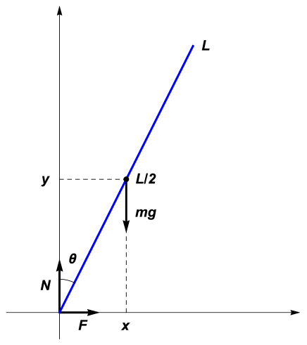
Figure 1: The falling pencil.

We will suppose for simplicity at first that the pencil is not allowed to move along the surface: for instance we can imagine it hinged at the axes origin and free to rotate without friction around it. We will also admit that it can go full circle – as if the table were not there – so that now $0\leq\theta\leq 2\pi$. This would enable us to study the reaction forces $N$ and $F$ in detail in an initially simplified setting that will be useful in the subsequent discussion. We have indeed in this case just a physical pendulum (an extended rigid body) performing swings of arbitrary amplitude. The topic is very well known and has been widely studied, for instance as inverted pendulum w.r.t. the stabilization of its equilibrium (see for instance [1], [2] and [3]): we will however skip these topics altogether by confining ourselves just to a simplified discussion of the circular pendulum.

The Newton equations of motion, with a fixed point in the origin, can be simply written in this case as

$$m\ddot{x}=F\qquad\quad m\ddot{y}=N-mg\quad\qquad I_{0}\ddot{\theta}=mgx=mg\frac{L}{2}\sin\theta$$ (2)

where $I_{0}=\,^{mL^{2}}/_{3}$ is the moment of inertia of the pencil w.r.t. its fixed end. Neglecting for the time being the first two equations, we focus our attention on the third that can be written as

$$\ddot{\theta}=\frac{\omega_{\perp}^{2}}{2}\,\sin\theta\qquad\quad\omega_{\perp}=\sqrt{\frac{3g}{L}}$$ (3)

There is not an explicit elementary solution of this non linear equation, but that notwithstanding we can study it in some detail. It is easy to see indeed that

$$\frac{d}{dt}\big{(}\dot{\theta}^{2}\big{)}=2\dot{\theta}\ddot{\theta}=\omega_{\perp}^{2}\,\dot{\theta}\sin\theta=-\omega_{\perp}^{2}\frac{d}{dt}\left(\cos\theta\right)$$

and therefore

$$\dot{\theta}^{2}=-\omega_{\perp}^{2}\,\cos\theta+c$$ (4)

where $c$ is an arbitrary integration constant depending on the initial conditions. Let us make at first (a bit naively) what seems to be the simplest choice, namely

$$\theta(0)=0\qquad\qquad\dot{\theta}(0)=0$$ (5)

In this case apparently we have $c=\omega_{\perp}^{2}$ and hence

$$\dot{\theta}^{2}=\omega_{\perp}^{2}(1-\cos\theta)\geq 0\qquad\quad 0\leq\theta\leq 2\pi$$

or in another form

$$\omega(\theta)=\frac{d\theta}{dt}=\omega_{\perp}\sqrt{1-\cos\theta}$$

This non-linear, first order equation – which also shows that $\omega_{\perp}$ is the angular velocity at $\theta=\,^{\pi}/_{2}$ – can be easily solved by separating the variables, namely

$$\int_{0}^{\theta}\frac{d\phi}{\sqrt{1-\cos\phi}}=\omega_{\perp}\int_{0}^{t}ds=\omega_{\perp}t$$

but it can be seen that the left hand integral diverges because the integrand function has a non integrable singularity in the origin:

$$\frac{1}{\sqrt{1-\cos\phi}}=O\big{(}\phi^{-1}\big{)}\qquad\quad\phi\to 0$$

We have indeed from L’Hôpital rule that

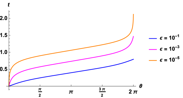
Figure 2: The time $t$ (in seconds) needed to reach an angle $\theta$ according to (9) for three different values of $\epsilon$ and $\omega_{\perp}=10\;\text{{sec}}^{-1}$ (corresponding to an $L$ of roughly $30$ cm). The pencil is allowed to go full circle from $0$ to $2\pi$.

$$\lim_{\phi\to 0}\frac{\phi}{\sqrt{1-\cos\phi}}=2\lim_{\phi\to 0}\frac{\sqrt{1-\cos\phi}}{\sin\phi}=2\lim_{\phi\to 0}\sqrt{\frac{1-\cos\phi}{1-\cos^{2}\phi}}=2\lim_{\phi\to 0}\frac{1}{\sqrt{1+\cos\phi}}=\sqrt{2}$$

As a matter of fact this behavior is rather understandable and can be traced back to our awkward choice of the initial conditions: when indeed we assume (5) we are putting the system in its position of unstable equilibrium, and therefore the pencil would ideally stand up forever so that the time needed to reach a position $\theta\neq 0$ would diverge. We need therefore to take a slightly different (and more realistic) initial condition, for instance with a gentle push onward

$$\theta(0)=0\qquad\qquad\dot{\theta}(0)=\omega_{0}>0$$ (6)

where $\omega_{0}$ can be chosen small and even infinitesimal to approach the ideal (but singular) condition (5). With this new assumption the integration constant in (4) becomes $c=\omega_{o}^{2}+\omega_{\perp}^{2}$ and the equation takes the form

$$\dot{\theta}^{2}=\omega_{0}^{2}+\omega_{\perp}^{2}(1-\cos\theta)$$ (7)

to wit

$$\omega(\theta)=\frac{d\theta}{dt}=\omega_{\perp}\sqrt{2\epsilon+1-\cos\theta}\qquad\qquad 2\epsilon=\frac{\omega_{0}^{2}}{\omega_{\perp}^{2}}$$

This equation can be solved again by separating the variables

$$\int_{0}^{\theta}\frac{d\phi}{\sqrt{1+2\epsilon-\cos\phi}}=\omega_{\perp}\int_{0}^{t}ds=\omega_{\perp}t$$ (8)

but now (see [4] 2.571.5) the left hand side integral converges for $\epsilon>0$ and we have

$$\sqrt{\frac{2}{1+\epsilon}}F\left(\arcsin\sqrt{(1+\epsilon)\frac{1-\cos\theta}{1+2\epsilon-\cos\theta}},\,\sqrt{\frac{1}{1+\epsilon}}\right)=\omega_{\perp}t$$ (9)

where (see [4] 8.111.2)

$$F(\varphi,b)=\int_{0}^{\varphi}\frac{d\alpha}{\sqrt{1-b^{2}\sin^{2}\alpha}}\qquad\quad b^{2}<1$$

is the elliptic integral of the first kind. As a matter of fact the equation (9) gives the function $\theta(t)$ in an implicit form that is not easy to invert, and this form moreover is not much more manageable than the original integral formulation (8) because the function $F(\varphi,b)$ is nothing else than a name for another integral. Since however these integrals are nowadays numerically performed by the usual mathematical software, the results (8) and (9) can easily be used to plot the function $t(\theta)$, time needed to reach an angle $\theta$, as in the Figure 2 where, with an exchange of the coordinate axes, we would also get a graphical representation of $\theta(t)$

We can next take advantage of the first two equations (2) to find the reaction forces $N$ and $F$: since from (1) it is

$$\ddot{x}=\frac{L}{2}\left(\ddot{\theta}\cos\theta-\dot{\theta}^{2}\sin\theta\right)\qquad\quad\ddot{y}=-\frac{L}{2}\left(\ddot{\theta}\sin\theta+\dot{\theta}^{2}\cos\theta\right)$$ (10)

from the first two equations in (2) we have

$$F=\frac{mL}{2}\left(\ddot{\theta}\cos\theta-\dot{\theta}^{2}\sin\theta\right)\qquad\quad N=mg-\frac{mL}{2}\left(\ddot{\theta}\sin\theta+\dot{\theta}^{2}\cos\theta\right)$$

and, since we know that, with the initial conditions (6), the equations (3) and (7) hold, after a little algebra we find how the reaction forces vary as functions of $\theta$

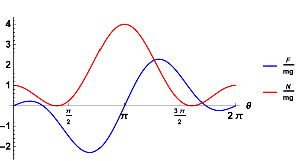
Figure 3: The dimensionless reaction forces $\,{}^{F}/_{mg}$ and $\,{}^{N}/_{mg}$ of (14) and (15) (for $\epsilon=0$) as functions of the position $\theta$.

$$F(\theta) = \frac{3\,mg}{2}\left(\frac{3}{2}\cos\theta-1-2\epsilon\right)\sin\theta$$ (11)

$$N(\theta) = \frac{mg}{4}+\frac{3\,mg}{2}\left(\frac{3}{2}\cos\theta-1-2\epsilon\right)\cos\theta$$ (12)

From (7) moreover it is also possible to show that the angular velocity $\omega=\dot{\theta}$ varies with the position $\theta$ according to the formula

$$\omega(\theta)=\omega_{\perp}\sqrt{2\epsilon+1-\cos\theta}$$ (13)

It is interesting to remark at this point that, while the time formula (8) is singular for $\epsilon\to 0^{+}$, the equations (11), (12) and (13) continuously go into their $\epsilon=0$ forms

$$F(\theta) = \frac{3\,mg}{2}\left(\frac{3}{2}\cos\theta-1\right)\sin\theta$$ (14)

$$N(\theta) = \frac{mg}{4}+\frac{3\,mg}{2}\left(\frac{3}{2}\cos\theta-1\right)\cos\theta$$ (15)

$$\omega(\theta) = \omega_{\perp}\sqrt{1-\cos\theta}$$ (16)

corresponding to the null initial conditions (5): these limiting formulas can now be properly used to represent the simplest behavior of the reaction forces and of the angular velocity at every possible position $\theta$. In the Figure 3 we have plotted the dimensionless functions $\,{}^{F}/_{mg}$ and $\,{}^{N}/_{mg}$ of (14) and (15) (with $\epsilon=0$), while the velocity (13) of (16) in its dimensionless form $\,{}^{\omega}/_{\omega_{\perp}}$ is plotted in the Figure 4 in the interval $[0,4\pi]$: for $\epsilon>0$, $\omega(\theta)$ turns out to be a smooth function even at the angles $\theta=0,2\pi,4\pi\ldots$ Apparently when we also plug into these formulas the function $\theta(t)$ implicitly defined in (9) we also get the time dependence of $F,N$ and $\omega$, but, needless to say, this would be a cumbersome task that we will neglect here

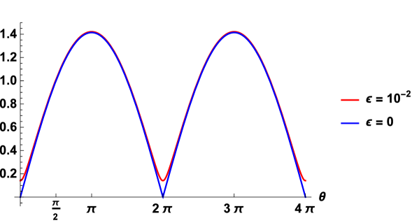
Figure 4: The dimensionless angular velocity ${}^{\omega}/_{\omega_{\perp}}$ of (13) as a function of $\theta$ for two different values of $\epsilon$.

It is worthwhile to remark finally that the two reaction components $N,$ and $F$ also take negative values: for $F$ this is apparent from the Figure 3 and we see from (14) that – even with $\epsilon=0$ and remaining just in the interval $[0,\,^{\pi}/_{2}]$ – we have $F<0$ provided that

$$\frac{2}{3}>\cos\theta\geq 0\qquad\arccos\left(\,{}^{2}/_{3}\right)<\theta\leq\frac{\pi}{2}\qquad\arccos\left(\,{}^{2}/_{3}\right)\simeq 0.268\,\pi$$

As for the normal component we find instead from (12) that $N$ can be negative only if $\epsilon>0$: more precisely we have $N\leq 0$ when

$$\frac{1}{3}+\frac{2}{3}\left(\epsilon+\sqrt{\epsilon(1+\epsilon)}\right)\geq\cos\theta\geq\frac{1}{3}+\frac{2}{3}\left(\epsilon-\sqrt{\epsilon(1+\epsilon)}\right)$$

namely for $\theta$ falling in an interval that shrinks to the single point $\arccos(\,^{1}/_{3})\simeq 0.392\,\pi$ for $\epsilon=0^{+}$. These negative values will be of some consequence in the sequel because they will suggest where an un-hinged pencil will begin a sliding movement when the available constraints will be unable to provide a negative reaction

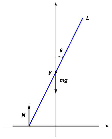
Figure 5: The pencil tip sliding along a frictionless rail.

3 Second movement: The rail

Before going ahead to our pencil with one end laid on a horizontal rough table and free to move along it, we will stop for a while to consider two more frictionless cases. In order to allow again for a full swing of the system from $0$ to $2\pi$, moreover, in the first of these examples we will suppose that the pencil tip on the $x$ axis in the Figure 5 is in fact constrained to slide along a rail without leaving it while the center of mass goes from $\,{}^{L}/_{2}$ to $\,{}^{-L}/_{2}$ and back again. At variance with the case of the previous section, however, now there is no horizontal force $F$ because neither friction nor hinges in the axes origin are present. As a consequence the pencil CM will simply move along the $y$ axis with $x=0$, if its movement starts with this initial condition. On the other hand there is no longer a fixed point of the system so that now its rotational dynamics is better accounted for by looking at its motion around the CM. Therefore the Newton equations now are

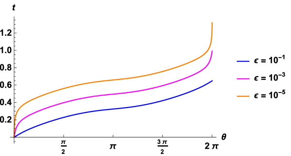
Figure 6: The time $t$ (in seconds) needed to reach an angle $\theta$ according to (23) for three different values of $\epsilon$ and $\omega_{\perp}=10\;\text{{sec}}^{-1}$. The pencil is allowed to go full circle from $0$ to $2\pi$.

$$m\ddot{x}=0\qquad\quad m\ddot{y}=N-mg\quad\qquad I_{CM}\ddot{\theta}=N\frac{L}{2}\sin\theta$$ (17)

where $I_{CM}=\,^{mL^{2}}/_{12}$ is the moment of inertia of the pencil w.r.t. its CM, while the geometrical relations among the coordinates become

$$x=0\qquad\qquad y=\frac{L}{2}\,\cos\theta$$ (18)

To tackle our problem we can now retrace a path similar to that followed in the Section 2: from (17) the rotational acceleration around the CM is

$$\ddot{\theta}=\frac{6N}{mL}\sin\theta$$ (19)

while on the other hand again from (17) and from (10) we find

$$N=m\left(\ddot{y}+g\right)=mg-\frac{mL}{2}\left(\ddot{\theta}\sin\theta+\dot{\theta}^{2}\cos\theta\right)$$ (20)

so that altogether it is

$$\ddot{\theta}=\sin\theta\left[2\omega_{\perp}^{2}-3\left(\ddot{\theta}\sin\theta+\dot{\theta}^{2}\cos\theta\right)\right]$$

It is easy to see now that

$$\frac{d}{dt}\big{(}\dot{\theta}^{2}\big{)} = 2\dot{\theta}\ddot{\theta}\;=\;2\dot{\theta}\sin\theta\left[2\omega_{\perp}^{2}-3\left(\ddot{\theta}\sin\theta+\dot{\theta}^{2}\cos\theta\right)\right]$$

$$= -\frac{d}{dt}\left[4\omega_{\perp}^{2}\cos\theta+3\left(\dot{\theta}\sin\theta\right)^{2}\right]$$

to wit

$$\dot{\theta}^{2}\left(1+3\sin^{2}\theta\right)+4\omega_{\perp}^{2}\cos\theta=c$$ (21)

and since with the slightly off-equilibrium initial conditions (6), and keeping the same notations, it is

$$c=4\omega_{\perp}^{2}+\omega_{o}^{2}=4\omega_{\perp}^{2}\left(1+\frac{\epsilon}{2}\right)\qquad\qquad\epsilon=\frac{\omega_{0}^{2}}{2\omega_{\perp}^{2}}$$

we finally have

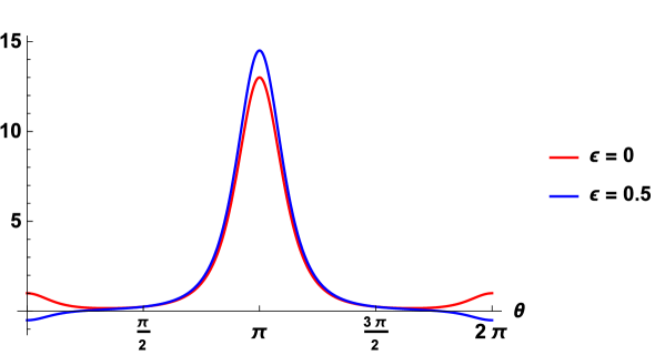
Figure 7: The dimensionless reaction force $\,{}^{N}/_{mg}$ of (24) and (25) as a function of the position $\theta$ for two values of $\epsilon$.

$$\dot{\theta}^{2}=\omega_{\perp}^{2}\,\frac{2\epsilon+4(1-\cos\theta)}{1+3\sin^{2}\theta}=\omega_{\perp}^{2}\,\frac{2\epsilon+4(1-\cos\theta)}{4-3\cos^{2}\theta}$$ (22)

This equation can be integrated again by separating the variables giving

$$\int_{0}^{\theta}\sqrt{\frac{4-3\cos^{2}\phi}{2\epsilon+4(1-\cos\phi)}}\,d\phi=\omega_{\perp}t=t\sqrt{\frac{3g}{L}}$$ (23)

and while this implicit solution has no elementary inverse function it is possible to numerically evaluate the integral to calculate the time $t$ needed to reach an angle $\theta$: the results plotted in the Figure 6 show a qualitative behavior similar to that of the Figure 2. Here too, however, the time $t$ diverges when $\epsilon\to 0^{+}$

To study next the reaction force $N$ we plug (19) and (22) into (20) obtaining the equation

$$N=mg-\frac{mL}{2}\left(\frac{6N}{mL}\sin^{2}\theta+\frac{3g}{L}\,\frac{2\epsilon+4(1-\cos\theta)}{1+3\sin^{2}\theta}\cos\theta\right)$$

that is easily solved providing

$$N=mg\,\frac{4+3\cos^{2}\theta-3(\epsilon+2)\cos\theta}{(4-3\cos^{2}\theta)^{2}}$$ (24)

For $\epsilon=0$ this simply becomes

$$N=mg\,\frac{4+3\cos^{2}\theta-6\cos\theta}{(4-3\cos^{2}\theta)^{2}}$$ (25)

The dimensionless function $\,{}^{N}/_{mg}$ is plotted in the Figure 7 for two different initial conditions $\epsilon$, and it is interesting to remark that now – at variance with the case discussed in the Section 2 – its values are always positive, and that to have also negative values the initial angular velocity $\omega_{0}$ should in fact exceed a fairly large threshold. More precisely it would be possible to see that the Mexican-hat shaped red curve of the Figure 7 bends its tails under the $x$-axis only for $\epsilon>\,^{1}/_{3}$, namely for $\omega_{0}>\sqrt{\,{}^{2g}/_{L}}\;\,\text{sec}^{-1}$: for example, for $L=0.2\;\text{m}$, this approximately means $\omega_{0}>10\;\text{sec}^{-1}$. Finally from (22) we have the angular velocity

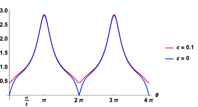
Figure 8: The dimensionless angular velocities $\,{}^{\omega}/_{\omega_{\perp}}$ of (26)and (27) as a function of $\theta$ for two values of $\epsilon$.

$$\omega(\theta)=\dot{\theta}=\omega_{\perp}\,\sqrt{\frac{2\epsilon+4(1-\cos\theta)}{1+3\sin^{2}\theta}}$$ (26)

that is for $\epsilon=0$

$$\omega(\theta)=2\omega_{\perp}\,\sqrt{\frac{1-\cos\theta}{1+3\sin^{2}\theta}}$$ (27)

In its dimensionless form $\,{}^{\omega}/_{\omega_{\perp}}$ this angular velocity is reproduced in the Figure 8 for two values of $\epsilon$, and the functions turn out to be smooth again even at $\theta=0,2\pi,4\pi,\ldots$ for every non-zero $\epsilon>0$

4 Third movement: The step

In our third frictionless case we begin first by looking back to the reaction forces discussed in the Section 2. When it begins to fall, indeed, the hinged pencil rotates as in the Figure 1 with a fixed point and hence the reaction forces vary with $\theta$ as in the Figure 3. To be more precise we have reproduced in the Figure 9 the forces $\,{}^{F(\theta)}/_{mg}$ and $\,{}^{N(\theta)}/_{mg}$ in the interval $0\leq\theta\leq\,^{\pi}/_{2}$ in the limiting case of $\epsilon=0$ presented in (14) and (15).

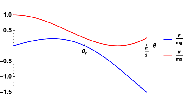
Figure 9: The dimensionless reaction forces $\,{}^{F}/_{mg}$ and $\,{}^{N}/_{mg}$ (14) and (15) of the hinged pencil of the Section 2 as functions of the position $0\leq\theta\leq\,^{\pi}/_{2}$ for $\epsilon=0$. From (14) we see that the force $F$ reverses its sign when $\theta\geq\theta_{r}=\arccos\,^{2}/_{3}$.

From this picture and the corresponding equations we see in particular that, while $N$ never goes negative, the horizontal component $F$ of the reactions in the Figure 1 reverses its sign beyond an angle $\theta_{r}=\arccos\,^{2}/_{3}\simeq 0.268\,\pi$ suggesting that some force is needed to keep the pencil tip from moving to the right when $\theta>\theta_{r}$. Suppose then now that – without being hinged at the origin – our pencil is just laid on a frictionless table and allowed to fall as in the Figure 1, but also that its contact tip is forbidden to slide leftwards (as instead it was allowed in the Section 3) by the presence of some obstacle, for instance a step as in the Figure 10. From the previous remarks it follows then that when $\theta$ exceeds $\theta_{r}$ the pencil tip starts sliding rightwards because – being now unhinged – no negative horizontal reaction force can arise to prevent that. The pencil reaches the angle $\theta_{r}$ at a time $t_{r}$ that can be explicitly calculated from the integral (8) for a small initial destabilizing condition $\epsilon>0$, while at that point its angular velocity from (16) is

$$\omega_{r}=\omega(\theta_{r})=\frac{\omega_{\perp}}{\sqrt{3}}=\sqrt{\frac{g}{L}}$$

We will now investigate the movement of our system for $\theta_{r}<\theta<\,^{\pi}/_{2}$ from the time $t_{r}$ until the instant $T$ of the impact on the table.

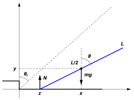
Figure 10: When $\theta>\theta_{r}=\arccos\,^{2}/_{3}$ on a frictionless surface with a step the pencil also starts drifting rightwards.

If, according to the Figure 10, $z$ is the position of the contact point on the table the relationships among the variables are now

$$x=z+\frac{L}{2}\,\sin\theta\qquad\quad y=\frac{L}{2}\,\cos\theta\qquad\qquad 0\leq\theta\leq\,^{\pi}/_{2}$$ (28)

while the Newton equations of motion are

$$m\ddot{x}=0\qquad\quad m\ddot{y}=N-mg\quad\qquad I_{CM}\ddot{\theta}=N\frac{L}{2}\sin\theta$$ (29)

where again $I_{CM}=\,^{mL^{2}}/_{12}$. As a consequence the second equation (10) together with the equations (19) and (20) still hold, and hence also (21) can be deduced. Imposing then the conditions at $t=t_{r}$ we find that the integration constant now is

$$c=\omega_{r}^{2}(1+3\sin^{2}\theta_{r})+3\omega_{\perp}^{2}\cos\theta_{r}=\frac{32}{9}\,\omega_{\perp}^{2}$$

and therefore we get

$$\dot{\theta}^{2}=\frac{4\,\omega_{\perp}^{2}}{9}\,\frac{8-9\cos\theta}{4-3\cos^{2}\theta}$$ (30)

with its new corresponding time equation

$$\int_{\theta_{r}}^{\theta}\sqrt{\frac{4-3\cos^{2}\phi}{8-9\cos\phi}}\,d\phi=\frac{2\,\omega_{\perp}}{3}\,(t-t_{r})$$ (31)

that can be numerically evaluated to calculate the time $t$ needed to reach an angle $\theta\in[\theta_{r},\,^{\pi}/_{2}]$: for instance the time $T$ when the pencil hits the floor will be

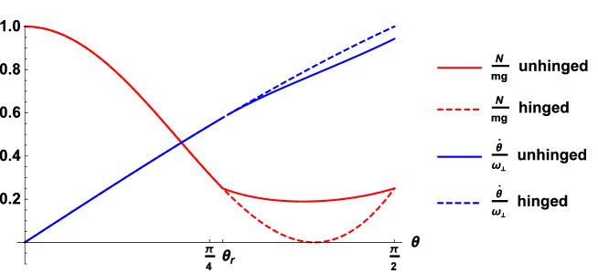
Figure 11: Dimensionless reaction force $\,{}^{N}/_{mg}$ and angular velocity $\,{}^{\dot{\theta}}/_{\omega_{\perp}}$ (continuous lines when $\theta\geq\theta_{r}$) on a frictionless surface with a step, compared with the same quantities in the case of the hinged pencil (dashed lines) that also accounts for the movement when $\theta<\theta_{r}$.

$$T=t_{r}+\frac{3}{2\omega_{\perp}}\int_{\theta_{r}}^{{}^{\pi}/_{2}}\sqrt{\frac{4-3\cos^{2}\phi}{8-9\cos\phi}}\,d\phi\simeq t_{r}+\frac{0.971}{\omega_{\perp}}\quad\qquad\omega_{\perp}=\sqrt{\frac{3g}{L}}$$ (32)

where $t_{r}$ comes from (8) choosing a small initial condition $\epsilon>0$. As for the reaction force $N$ on the other hand, from (19), (20) and (30) we have that

$$N=mg-\frac{mL}{2}\left(\frac{6N}{mL}\sin^{2}\theta+\frac{4g}{3L}\,\frac{8-9\cos\theta}{4-3\cos^{2}\theta}\cos\theta\right)$$

that eventually gives

$$N=mg\,\frac{3\cos^{2}\theta-\frac{16}{3}\cos\theta+4}{(4-3\cos^{2}\theta)^{2}}$$ (33)

The plot of $\,{}^{N}/_{mg}$ in the Figure 11 shows in particular that $N$ always stays positive even in the interval $[\theta_{r},\,^{\pi}/_{2}]$ signaling that the pencil tip never leaves the table surface. In the same Figure 11 also the dimensionless angular velocity $\,{}^{\dot{\theta}}/_{\omega_{\perp}}$ is displayed in the same interval.

To investigate next the behavior of $x,y$ and $z$ of (28) we begin by remarking that the first equation in (29), $m\ddot{x}=0$, clearly entails that $\dot{x}=c$ for $t\geq t_{r}$, while to find the integration constant $c$ it is enough to remark that

$$\dot{x}(t)=c=\dot{x}(t_{r})=\frac{L}{2}\,\omega_{r}\cos\theta_{r}=\frac{\omega_{\perp}L}{3\sqrt{3}}\qquad\quad t_{r}\leq t\leq T$$ (34)

As a consequence we will have

$$x(t)=\frac{L}{2}\,\cos\theta_{r}+\frac{\omega_{\perp}L}{3\sqrt{3}}(t-t_{r})=\frac{L}{3}+\frac{\omega_{\perp}L}{3\sqrt{3}}(t-t_{r})\qquad\quad t_{r}\leq t\leq T$$

The chronological equations of $y$ and $z$, instead, can not be deduced so simply: the second equations (29) for $y$, for instance, would be nothing new w.r.t. the angular equation, in the sense that if we know $\theta(t)$ we also can find $y(t)$ by taking advantage of the second equation (28). But we have seen that the angular equation (30) can not be integrated in an elementary way, and hence even $y(t)$ has not a manageable form. Shunning however this chronological issue, we can at least gain some insight into the shape of the trajectory of the CM of coordinates $x$ and $y$.

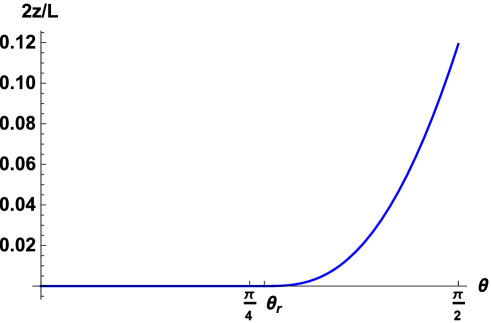
Figure 12: Dimensionless position $\,{}^{2z(\theta)}/_{L}$ of the pencil tip laid on a frictionless table with a step, as a function of $\theta$: as long as $\theta\leq\theta_{r}$ it is $\,{}^{2z(\theta)}/_{L}=0$, but when $\theta\geq\theta_{r}$ the function $z(\theta)=\zeta(\cos\theta)$ should be calculated from (36).

It is apparent indeed that until the sliding begins (namely when $0\leq t\leq t_{r}$ and $0\leq\theta\leq\theta_{r}$) the CM follows a circular path of radius $\,{}^{L}/_{2}$ around the origin; as soon as $t>t_{r}$ and $\theta>\theta_{r}$, however, the CM parts way from the aforementioned circumference following a different flight that can be scrutinized by looking again into the equations (28): by eliminating indeed $\cos\theta$ between the equations

$$(x-z)^{2}=\frac{L^{2}}{4}\sin^{2}\theta=\frac{L^{2}}{4}(1-\cos^{2}\theta)\qquad\quad y^{2}=\frac{L^{2}}{4}\cos^{2}\theta$$

we have

$$y=\sqrt{\frac{L^{2}}{4}-(x-z)^{2}}$$

pointing to the fact that now the CM treads along a circle, but with a moving center in $z$. The $t$-parametric equations of this trajectory then are

$$x(t)=z(t)+\frac{L}{2}\sqrt{1-\cos^{2}\theta(t)}\qquad\quad y(t)=\frac{L}{2}\,\cos\theta(t)$$

and if we define a function $\zeta(s)$ such that

$$z(t)=\zeta\big{(}s(t)\big{)}\qquad\quad s(t)=\cos\theta(t)$$

by adopting $s$ as a new parameter the parametric equations become

$$x(s)=\zeta(s)+\frac{L}{2}\sqrt{1-s^{2}}\qquad\quad y(s)=\frac{L}{2}\,s\qquad\quad s=\cos\theta\in[0,1]$$ (35)

We are therefore prompted to study $\zeta(s)$: from (28), (30) and (34) we know that

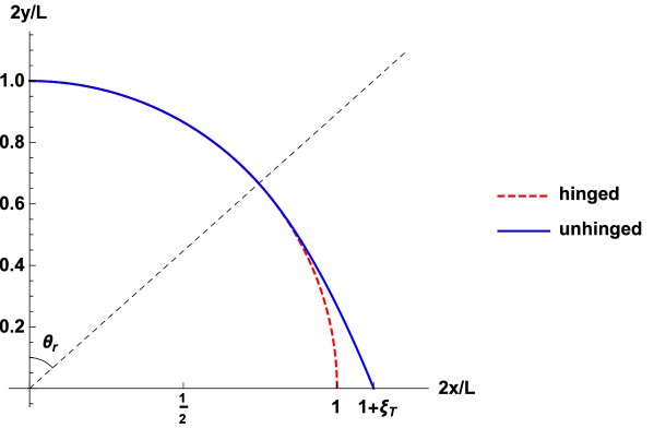
Figure 13: Dimensionless CM $xy$-trajectory: it coincides with the circular path of the hinged pencil for $\theta\leq\theta_{r}$, but as soon as $\theta\geq\theta_{r}$ it follows a different flight with the parametric equations (35).

$$\dot{z}=\dot{x}-\frac{L}{2}\,\dot{\theta}\cos\theta=\frac{\omega_{\perp}L}{3\sqrt{3}}\left(1-\sqrt{3\cos^{2}\theta\,\frac{8-9\cos\theta}{4-3\cos^{2}\theta}}\right)$$

and since $\dot{z}=\zeta\,^{\prime}(s)\,\dot{s}=-\zeta^{\prime}(s)\,\dot{\theta}\sin\theta$, using (30) again we find

$$\zeta\,^{\prime}(s)=-\frac{L}{2\sqrt{3}}\left(\sqrt{\frac{4-3s^{2}}{(1-s^{2})(8-9s)}}-\sqrt{\frac{3s^{2}}{1-s^{2}}}\right)\qquad\quad 0\leq s\leq\,^{2}/_{3}$$

namely

$$\zeta(s)=\frac{L}{2\sqrt{3}}\int_{s}^{\,{}^{2}/_{3}}\left(\sqrt{\frac{4-3u^{2}}{(1-u^{2})(8-9u)}}-\sqrt{\frac{3u^{2}}{1-u^{2}}}\right)du\qquad\quad 0\leq s\leq\,^{2}/_{3}$$ (36)

This integral, that can be performed at least numerically, lends now the possibility of plotting both $z(\theta)=\zeta(\cos\theta)$ (Figure 12), and the trajectory parametric equations (35) (Figure 13) where it is understood that $\zeta(s)=0$ when $\,{}^{2}/_{3}\leq s\leq 1$. Remark that from (36) we can also assess the value $x_{T}$ of $x$ when the pencil finally hits the floor: if $T$, as provided by (32), is the impact time, we of course have $\theta(T)=\,^{\pi}/_{2}$, namely $s(T)=0$ and therefore the CM $x$-coordinate when the pencil lands on the table is

$$x_{T}=z_{T}+\frac{L}{2}=\frac{L}{2}(1+\xi_{T})\qquad\quad z_{T}=z(T)=\zeta\left(s(T)\right)=\zeta(0)=\frac{L}{2}\,\xi_{T}$$

where

$$\xi_{T}=\frac{1}{\sqrt{3}}\int_{0}^{\,{}^{2}/_{3}}\left(\sqrt{\frac{4-3u^{2}}{(1-u^{2})(8-9u)}}-\sqrt{\frac{3u^{2}}{1-u^{2}}}\right)du\simeq 0.12$$

can be numerically evaluated: if for instance $L=20\;\text{cm}$, this roughly means that $z_{T}\simeq 1.2\;\text{cm}$

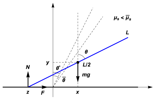
Figure 14: The pencil tip on the table starts to drift leftward past an angle $\theta^{*}<\overline{\theta}=\arccos\,^{9}/_{11}\simeq 0.195\,\pi$ if the static friction coefficient is not large enough ($\mu_{s}<\overline{\mu}_{s}\simeq 0.37$) to forbid it.

5 Fourth movement: The rough surface

We finally go back to our initial problem of a pencil with one end laid on a horizontal rough table and free to slide along it while falling, Because of the presence of friction, when the pencil starts its movement the extremity in contact with the surface does not move, but it can possibly slide (on both sides as we shall see) at a later time $t^{*}$ when it passes beyond a position $\theta^{*}$: to understand how this happens we must therefore first of all look again at the reaction forces discussed in the Section 2 and 4. When it begins to fall, indeed, the pencil rotates as in the Figure 1 with a fixed point and hence the reaction forces – in the limiting case of $\epsilon=0$ presented in (14) and (15) – vary with $\theta$ as in the Figure 9 with $0\leq\theta\leq\,^{\pi}/_{2}$. We already remarked in the Section 4 that $F$ (the horizontal component of the reactions in the Figure 1) is supposed to reverse its sign beyond an angle $\theta_{r}=\arccos\,^{2}/_{3}\simeq 0,268\,\pi$ (suggesting that some force is needed to keep the pencil tip from moving to the right when $\theta>\theta_{r}$), but only if it does not start to slide to the left at an earlier time $t^{*}$ at an angle $\theta^{*}$ as in the Figure 14. This second occurrence must indeed be taken into account because now – in absence of the step of the Section 4 – the static friction force must always satisfy the condition $|F|\leq\mu_{s}N$, and it may happen that this requirement is not met beyond some angle $\theta^{*}<\theta_{r}$.

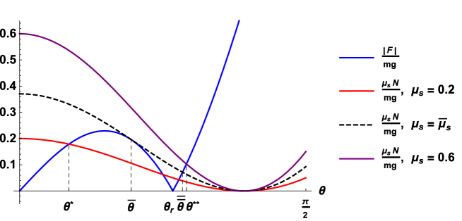
Figure 15: The absolute value of the friction forces $\,{}^{|F|}/_{mg}$ may exceed its maximum $\,{}^{\mu_{s}N}/_{mg}$ at several possible angles according to the value of $\mu_{s}$. If $\mu_{s}<\overline{\mu}_{s}$ a slipping takes place toward the left beyond an angle $\theta^{*}$; when instead $\mu_{s}>\overline{\mu}_{s}$ the pencil tip starts sliding toward the right at a later time past the angle $\theta^{**}$.

In order to understand if and when this happens, a (dimensionless) comparison between $|F|$ and $\mu_{s}N$ has been displayed in the Figure 15 wherefrom we see that whenever $\mu_{s}$ is smaller than a critical value $\overline{\mu}_{s}$ the pencil starts slipping to the left at an angle $\theta^{*}$. From the equation (8) it is also possible to find the time $t^{*}$ of this occurrence for every non zero initial condition $\epsilon>0$. When instead $\mu_{s}>\overline{\mu}_{s}$, the slipping happens toward the right at a later time $t^{**}$ when the absolute value of the (now reversed) friction force exceeds the critical value at a larger angle $\theta^{**}$.

To find the numerical values of these quantities we must first of all look (with a given $\mu_{s}$) for the values of the angle $\theta$ such that $|F|=\mu_{s}N$ namely, from (14) and (15), such that

$$\left|\frac{3}{2}\left(\frac{3}{2}\cos\theta-1\right)\sin\theta\,\right|=\mu_{s}\left(\frac{1}{4}+\frac{3}{2}\left(\frac{3}{2}\cos\theta-1\right)\cos\theta\right)$$ (37)

when $0\leq\theta\leq\,^{\pi}/_{2}$. Squaring both sides and defining for simplicity $s=\cos\theta\in[0,1]$, after a little algebra the previous equation becomes

$$(1-s^{2})(9s-6)^{2}=\mu_{s}^{2}(3s-1)^{4}$$ (38)

and to search for its solutions in $[0,1]$ we recast it in the form

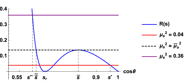
Figure 16: The solutions of the equation (38) correspond to the values of $s=\cos\theta$ such that $R(s)=\mu_{s}^{2}$. The critical friction coefficient $\overline{\mu}_{s}$ – beyond which no left-slipping takes place – coincides with the maximum of $R(s)$. The particular values and the notation are carried over from those of the Figure 15.

$$R(s)=\frac{(1-s^{2})(9s-6)^{2}}{(3s-1)^{4}}=\mu_{s}^{2}$$ (39)

that is represented in the Figure 16 with the same values of $\mu_{s}$ adopted in the Figure 15. It is apparent therefrom that $s^{*}=\cos\theta^{*}$ and $s^{**}=\cos\theta^{**}$ are the values for slipping toward the left and toward the right respectively, while $s_{r}=\cos\theta_{r}=\,^{2}/_{3}$ corresponds to the sign inversion of $F$ in the case of the hinged pencil discussed in the Section 2. The critical value $\overline{\mu}_{s}$ of the friction coefficient, beyond which no left-slipping is possible, can moreover be deduced as the maximum value of $R(s)$ by requiring that $R\,^{\prime}(s)=0$: a little algebra would show indeed that the maximum of $R(s)$ is attained at $\overline{s}=\,^{9}/_{11}$, namely at $\overline{\theta}=\arccos\,^{9}/_{11}\simeq 0.195\,\pi$ corresponding to the following critical value of the static coefficient of friction

$$\overline{\mu}_{s}^{2}=R\left(\,{}^{9}/_{11}\right)=2^{-13}3^{2}5^{3}\simeq 0.1373\qquad\quad\overline{\mu}_{s}=\frac{15}{64}\sqrt{\frac{5}{2}}\simeq 0.3706$$ (40)

The values of the slipping angles $\theta^{*},\theta^{**}$ can finally be deduced by numerically solving the equation (38): it is easy to show for instance that with the values of $\mu_{s}$ used in the Figures 15 and 16 we would have

$$\mu_{s}=0.20<\overline{\mu}_{s}\simeq 0.37 \cos\theta^{*}\simeq 0.964\;\qquad\theta^{*}\simeq 0.086\,\pi$$

$$\mu_{s}=0.60>\overline{\mu}_{s}\simeq 0.37 \cos\theta^{**}\simeq 0.609\qquad\theta^{**}\simeq 0.292\,\pi$$

It is also possible to see by direct calculation that at the critical friction coefficient $\overline{\mu}_{s}$ of (40) the equation (39) in $[0,1]$ also has its smallest solution in

$$\overline{\overline{s}}=\frac{48\sqrt{14}-35}{231}$$

corresponding to the the largest solution of (37)

$$\overline{\overline{\theta}}=\arccos\frac{48\sqrt{14}-35}{231}\simeq 0.285\,\pi$$

By summarizing: the limiting angles are

$$0<\overline{\theta}<\theta_{r}<\overline{\overline{\theta}}<\,^{\pi}/_{2}\qquad\left\{\begin{array}[]{l}\overline{\theta}=\arccos\,^{9}/_{11}\simeq 0.195\,\pi\\ \theta_{r}=\arccos\,^{2}/_{3}\simeq 0.268\,\pi\\ \overline{\overline{\theta}}=\arccos\frac{48\sqrt{14}-35}{231}\simeq 0.285\,\pi\end{array}\right.$$

and when $\mu_{s}<\overline{\mu}_{s}$ the pencil tip slips leftwards past an angle $\theta^{*}\leq\overline{\theta}$, while if $\mu_{s}>\overline{\mu}_{s}$ a rightward sliding starts only later beyond an angle $\theta^{**}\geq\overline{\overline{\theta}}$: the particular values of $\theta^{*}$ and $\theta^{**}$ depend on $\mu_{s}$ and can be calculated numerically from the equation (38). It also goes without saying that $\theta^{*}$ grows from $0$ to $\overline{\theta}$ when $\mu_{s}$ grows from $0$ to $\overline{\mu}_{s}$, while subsequently $\theta^{**}$ starts growing from $\overline{\overline{\theta}}>\overline{\theta}$ when $\mu_{s}$ exceeds $\overline{\mu}_{s}$: no slipping angle (either $\theta^{*}$ or $\theta^{**}$) can be found instead in the interval $[\overline{\theta},\overline{\overline{\theta}}\,]$, namely between $\arccos\,^{9}/_{11}\simeq 0.195\,\pi$ and $\arccos\frac{48\sqrt{14}-35}{231}\simeq 0.285\,\pi$

Beyond these slipping angles, either $\theta^{*}$ or $\theta^{**}$, the pencil dynamics is rather different and we will study in some detail only the case $\mu_{s}<\overline{\mu}_{s}$ with a leftward slipping beyond $\theta^{*}$ represented in the Figure 14: the case $\mu_{s}>\overline{\mu}_{s}$ with a rightward slipping beyond $\theta^{**}$ is not really different ad its discussion – combining elements of the following treatment and of the case of Section 4 – is left to the interested reader. When $\mu_{s}<\overline{\mu}_{s}$ we already know that the leftward sliding of the pen tip begins past an angle $\theta^{*}=\arccos s^{*}$ where $s^{*}$ is the largest solution of the equation (38) in $[0,1]$. We also know that this happens at a time $t^{*}$ that can be calculated from (8) with $\theta=\theta^{*}$ and in fact depends on the initial conditions: we recall from the discussion of the Section 2 that in fact $t^{*}$ diverges when we choose the zero initial condition $\epsilon\to 0^{+}$, but also that this is not an insurmountable hindrance if we leave aside the complete chronological equations and focus instead on the trajectory shape.

In order to analyze the movement in the intervals $t^{*}\leq t\leq T$ and $\theta^{*}\leq\theta\leq\,^{\pi}/_{2}$ we recall first that the coordinates of the system of Figure 14 still satisfy the relations (28) where however we now have $z=0$ for $0\leq\theta\leq\theta^{*}$, and $z\leq 0$ for $\theta^{*}\leq\theta\leq\,^{\pi}/_{2}$. If moreover $\mu_{\kappa}$ is the kinetic coefficient of friction between the pencil and the rough surface, the Newton equations of motion now are

$$m\ddot{x}=\mu_{\kappa}N\qquad\quad m\ddot{y}=N-mg\quad\qquad I_{CM}\ddot{\theta}=N\frac{L}{2}\sin\theta$$ (41)

with $I_{CM}=\,^{mL^{2}}/_{12}$: these equations coincide with the (29) of Section 4 but for the first one that now accounts for the kinetic friction force. Therefore the second equation (10) and the equations (19) and (20) still hold and hence we can deduce the equation (21) again as we did in the Sections 3 and 4: here however, to find the integration constant $c$, we must impose new conditions at $t=t^{*}$. We have indeed first from (16) that

$$\theta(t^{*})=\theta^{*}\qquad\quad\dot{\theta}(t^{*})=\omega^{*}=\omega(t^{*})=\omega_{\perp}\sqrt{1-\cos\theta^{*}}\qquad\quad\omega_{\perp}=\sqrt{\frac{3g}{L}}$$

and then that

$$x(t^{*})=\frac{L}{2}\sin\theta^{*} \dot{x}(t^{*})=\frac{L}{2}\omega_{\perp}\cos\theta^{*}\sqrt{1-\cos\theta^{*}}$$

$$y(t^{*})=\frac{L}{2}\cos\theta^{*} \dot{y}(t^{*})=-\frac{L}{2}\omega_{\perp}\sin\theta^{*}\sqrt{1-\cos\theta^{*}}$$

$$z(t^{*})=0 \dot{z}(t^{*})=0$$

We are therefore able to calculate $c$ and after a little algebra we find

$$\dot{\theta}^{2}=\frac{4\,\omega_{\perp}^{2}}{9}\,\frac{9-\frac{27}{4}\cos^{2}\theta^{*}(1-\cos\theta^{*})-9\cos\theta}{4-3\cos^{2}\theta}$$ (42)

that replaces (30) with its corresponding time equation which is now

$$\int_{\theta^{*}}^{\theta}\sqrt{\frac{4-3\cos^{2}\phi}{9-\frac{27}{4}\cos^{2}\theta^{*}(1-\cos\theta^{*})-9\cos\phi}}\,d\phi=\frac{2\,\omega_{\perp}}{3}\,(t-t^{*})$$ (43)

This integral can be numerically evaluated to calculate the time $t$ needed to reach an angle $\theta\in[\theta^{*},\,^{\pi}/_{2}]$: for instance, if we take $\cos\theta^{*}=0.95>\,^{9}/_{11}=\cos\overline{\theta}$ (that corresponds to $\mu_{s}\simeq 0.233<0.371=\overline{\mu}_{s}$), the time $T$ when the pencil hits the floor now becomes

$$T=t^{*}+\frac{3}{2\omega_{\perp}}\int_{\theta^{*}}^{\,{}^{\pi}/_{2}}\sqrt{\frac{4-3\cos^{2}\phi}{9-\frac{27}{4}\cos^{2}\theta^{*}(1-\cos\theta^{*})-9\cos\phi}}\,d\phi\simeq t^{*}+\frac{2.029}{\omega_{\perp}}$$ (44)

where $t^{*}$ comes from (8) choosing a small initial condition $\epsilon>0$. As for the reaction force $N$ on the other hand, from (41) (namely (19) and (20) as in the Sections 3 and 4) and from (42) we have now

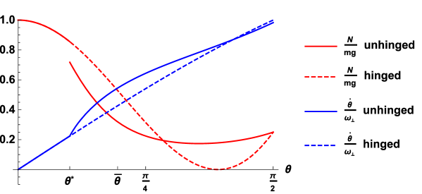
Figure 17: Dimensionless reaction force $\,{}^{N}/_{mg}$ and angular velocity $\,{}^{\dot{\theta}}/_{\omega_{\perp}}$ (continuous lines) on a rough surface with $\mu_{s}<\overline{\mu}_{s}$, compared with the same quantities in the case of the hinged pencil (dashed lines): the values coincide when $\theta<\theta^{*}$. Here we took $\cos\theta^{*}=0.95$ corresponding to $\mu_{s}\simeq 0.233$

$$N=mg\,\frac{3\cos^{2}\theta-\big{[}6-\frac{9}{2}(1-\cos\theta^{*})\cos^{2}\theta^{*}\big{]}\cos\theta+4}{(4-3\cos^{2}\theta)^{2}}\quad\qquad\theta^{*}\leq\theta\leq\,^{\pi}/_{2}$$ (45)

while for $0\leq\theta\leq\theta^{*}$ it takes the same values of the hinged case of Section 2. The plot of $\,{}^{N}/_{mg}$ in the Figure 17 shows in particular that $N$ is discontinuous at $\theta^{*}$ signaling the transition from the static to the kinetic friction. In the same Figure 17 also the dimensionless angular velocity $\,{}^{\dot{\theta}}/_{\omega_{\perp}}$ is displayed in the same intervals.

We come finally to give some detail about the CM trajectory and the position $z$ of the tip, but at variance with the discussion of the Section 4, $\dot{x}(t)$ no longer is a constant as in (34) since we must now take into account the kinetic friction force in the first equation (41). A quest for a simple chronological equation $x(t)$, however, would still be doomed because of the rather involuted form (45) of $N$. We can nevertheless gain some insight into the trajectories by looking again to our quantities rather as functions of the angle $\theta$, as we already did in the previous sections. While apparently for $0\leq\theta\leq\theta^{*}$ it is $z=0$ and the CM follows a circular path of radius $\,{}^{L}/_{2}$ around the origin, as soon as $\theta>\theta^{*}$ it will follow a path of parametric equations (35) with $\zeta(s)=0$ for $s=\cos\theta\in[s^{*},1]$ ($s^{*}=\cos\theta^{*}$): in order to complete the trajectory we are therefore left just with the task of calculating $\zeta(s)$ for $s\in[0,s^{*}]$. In order to do that we first remark that from (28) we have

$$\dot{z}=\dot{x}-\frac{L}{2}\dot{\theta}\cos\theta$$

On the other hand, within the notations of the Section 4 with $s=\cos\theta$, it is

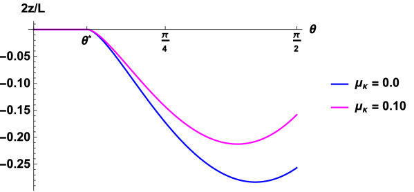
Figure 18: Dimensionless position $\,{}^{2z(\theta)}/_{L}$ of the pencil tip laid on a rough table for two different kinetic friction coefficients $\mu_{k}$, as a function of $\theta$: as long as $\theta\leq\theta^{*}$ it is $\,{}^{2z(\theta)}/_{L}=0$, but when $\theta\geq\theta^{*}$ the function $z(\theta)=\zeta(\cos\theta)$ should be calculated from (48): its value is now in the negative. Here again we have chosen $\cos\theta^{*}=0.95$.

$$\dot{z}=\zeta\,^{\prime}\dot{s}=-\zeta\,^{\prime}\dot{\theta}\sin\theta=-\zeta\,^{\prime}\dot{\theta}(s)\sqrt{1-s^{2}}$$

so that, defining a function $v(s)$ such that $\dot{x}(t)=v\big{(}s(t)\big{)}$, we get

$$\zeta\,^{\prime}(s)=-\frac{v(s)}{\dot{\theta}(s)\sqrt{1-s^{2}}}+\frac{L}{2}\,\frac{s}{\sqrt{1-s^{2}}}\qquad\quad\zeta(s^{*})=0$$ (46)

We see moreover from the definitions that

$$\ddot{x}=v^{\prime}\dot{s}=-v^{\prime}(s)\dot{\theta}(s)\sqrt{1-s^{2}}$$

and hence the first dynamical equation (41) becomes

$$v^{\prime}(s)=-\frac{\mu_{\kappa}}{m}\,\frac{N(s)}{\dot{\theta}(s)\sqrt{1-s^{2}}}\qquad\quad v(s^{*})=v^{*}=\frac{L\,\omega_{\perp}}{2}s^{*}\sqrt{1-s^{*}}$$

to wit

$$v(s)=v^{*}+\frac{\mu_{\kappa}}{m}\int_{s}^{s^{*}}\frac{N(r)}{\dot{\theta}(r)\sqrt{1-r^{2}}}\,dr$$ (47)

By assembling (46) and (47) we finally have

$$\zeta(s)=\int_{s}^{s^{*}}\left[\frac{1}{\dot{\theta}(q)\sqrt{1-q^{2}}}\left(v^{*}+\frac{\mu_{\kappa}}{m}\int_{q}^{s^{*}}\frac{N(r)}{\dot{\theta}(r)\sqrt{1-r^{2}}}\,dr\right)-\frac{L}{2}\,\frac{q}{\sqrt{1-q^{2}}}\right]dq$$ (48)

where, with $\beta^{*}=s^{*}\sqrt{1-s^{*}}$, it is understood from (42) and (45) that

$$\dot{\theta}(s)=\omega_{\perp}\sqrt{\frac{4-3\beta^{*\,2}-4s}{4-3s^{2}}}\qquad\quad N(s)=mg\frac{6s^{2}-3(4-3\beta^{*\,2})s+8}{2(4-3s^{2})}$$

The integral (48) can be calculated numerically and lends again the possibility of plotting both $z(\theta)=\zeta(\cos\theta)$ (Figure 18), and the trajectory parametric equations (35) together with (48) (Figure 19) where it is understood that $\zeta(s)=0$ when $s^{*}\leq s\leq 1$. In both the plots we have chosen $\theta^{*}=\arccos 0.95$ (corresponding to the static coefficient of friction $\mu_{s}\simeq 0.233$), and two possible values for the kinetic coefficient of friction: the limiting value $\mu_{\kappa}^{0}=0.0$ and $\mu_{\kappa}=0.10\,$. Remark that now, at variance with what we have found in the similar discussion of the Section 4, $z(s)$ takes negative values for $0\leq s\leq s^{*}$ accounting for the fact that the pencil tip slides leftward. From (48) we can also calculate the point $x_{T}$ where the pencil CM hits the floor at the time $T$: since it is $\theta(T)=\,^{\pi}/_{2}$, namely $s(T)=0$ we will have

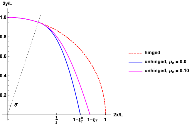
Figure 19: Dimensionless CM $xy$-trajectory: it coincides with the circular path of the hinged pencil for $\theta\leq\theta^{*}$, but as soon as $\theta\geq\theta^{*}$ it follows different flight according to the kinetic coefficient of friction: the parametric equations are (35) together with (48) to calculate $\zeta(s)$.

$$x_{T}=z_{T}+\frac{L}{2}=\zeta(0)+\frac{L}{2}=\frac{L}{2}(1-\xi_{T})\qquad\quad\xi_{T}=-\frac{2\zeta(0)}{L}\geq 0$$

where, with $\theta^{*}=\arccos 0.95$, it is

$$\left\{\begin{array}[]{ll}\xi_{T}^{0}\simeq 0.257,&\quad\hbox{for $\mu_{\kappa}^{0}=0.0$}\\ \xi_{T}\simeq 0.158,&\quad\hbox{for $\mu_{\kappa}=0.10$}\end{array}\right.$$

6 Epilogue

In this paper we have given an elementary treatment of a mechanical case study: the dynamics of a pencil with a tip laid on a rough table and set free to fall under the action of gravity. Despite its seeming modesty and lack of pretention we have shown that a discussion of this simple problem still conceals many details of (maybe) unexpected – but never unsurmountable – intricacy that may turn out to be pedagogically edifying. Along our exploration we also had the occasion to point out a few small results of a broader scope, as for instance some critical values of the sliding angles and of the static coefficients of friction. We hope that this Divertimento could eventually prove to be both profitable and entertaining for all those willing to stop for a while to listen at it

References

[1]G.F. Franklin, J.D. Powell and A. Emami-Naeini, Feedback Control of Dynamic Systems
(Pearson, Boston 2015)
[2]D. Liberzon, Switching in Systems and
Control (Birkhäuser, Boston, 2003)