Superconducting critical temperature in the extended diffusive SYK model

Abstract

Models for strongly interacting fermions in disordered clusters forming an array, with electron hopping between sites, reproduce the linear dependence on temperature of the resistivity, typical of the strange metal phase of High Temperature Superconducting materials (Extended Sachdev-Ye-Kitaev (SYK) models). We identify the low energy collective excitations as neutral, energy excitations, diffusing in the lattice of the thermalized, non Fermi liquid phase. However, the diffusion is heavily hindered by coupling to the pseudo Goldstone modes of the conformal broken symmetry SYK phase, which are local in space. The imaginary time evolution of the extended model in the strong interaction and $1/N$ expansion limit is presented, in the incoherent non chaotic regime. On the other hand, a Fermi electronic liquid at low energy becomes marginal when perturbed by the SYK dots. A critical temperature for superconductivity is derived, which is not BCS-like, in case the collective excitations are assumed to mediate an attractive Cooper-pairing.

I Introduction

Understanding the physics of copper-oxide materials, which undergo the superconducting transition at higher temperature, is still an unsettled topic of Condensed Matter Physics. Recent work suggests the breakdown of the Fermi Liquid (FL) theory at intermediate temperatures in these metals, while FL is the conventional starting point for low critical temperature superconductivity Hill et al. (2001); Jain and Anderson (2009). New approaches to study high-temperature superconductivity are recently investigated, in particular lattice fermionic models with a strong local interaction Chowdhury and Berg (2020a); Lantagne-Hurtubise et al. (2021).

Recently a $(0+1)-$ dimensional model, the Sachdev-Ye-Kitaev (SYK)Sachdev and Ye (1993); Kitaev ; Kitaev and Suh (2018) model, describing random all-to-all ${\cal{J}}-$interaction between $N$ Majorana fermions, has been extensively studied. In the infrared (IR) limit, when $N$ is large and the temperature $T$ is low, the model has an emergent approximate conformal symmetry and has become quite popular for its large-$N$ "melons" diagrammatics, which allows for a simple representation of the power-law decay in time of the correlation functions and for the analysis of the thermodynamic and chaotic propertiesKitaev and Suh (2018); Maldacena and Stanford (2016), providing a holographic dual for gravity theoriesSachdev (2010); Diaz et al. (2018).

Generalized SYK models have been proposed with extension to higher space dimensions Gu et al. (2017); Davison et al. (2017); Song et al. (2017); Berkooz et al. (2017); Chew et al. (2017); Haldar and Shenoy (2018); Patel et al. (2018a); Chowdhury et al. (2018) also having in mind applications to High Critical Temperature ($HT_{c}$) superconducting materials. Indeed, there seems to be widespread consensus that inhomogeneity and strong coupling could be distinguished factors for the cuprates and their $2-d$ $CuO$ planes. Moreover, universal features emerge in the high temperature "strange metal" phase, which is recognized as a Non Fermi Liquid (NFL) phaseParcollet and Georges (1999); Hill et al. (2001); Varma et al. (2002); Jain and Anderson (2009); Ben-Zion and McGreevy (2018); Patel et al. (2018b). The most striking of these is the linear increase with temperature of the electrical conductivityGurvitch and Fiory (1987); Daou et al. (2008); Cha et al. (2020a).

The conformal symmetry of the SYK model is spontaneously broken down to the $\widetilde{SL}(2,\mathbb{R})$ group symmetryKitaev (2018) and Goldstone modes arise which are only approximately gapless, when ultraviolet (UV) corrections are taken into account. The nature and the role of these collective excitations has not been satisfactorily investigated, to our knowledge, up to now, in phenomenological approaches for the description of the low temperature metal phases of extended SYK modelsGu et al. (2017).

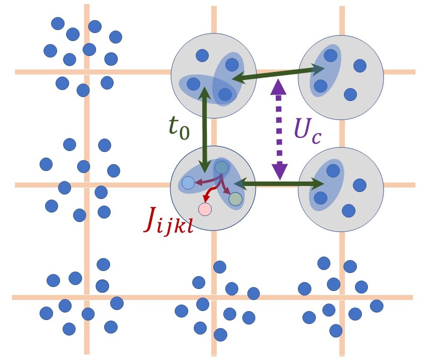
Figure 1: A cartoon of the SYK model extended to include hopping between $2-d$ square lattice sites. The neutral fermions are depicted as small blue circles, grouped on the lattice sites (their number is $N$ on each site). In the right upper part of the picture, a magnification of four sites with just four Majorana particles at each site, to represent the all-to-all four fermion interaction $J_{ijkl}$ [red arrows] and the residual interaction $U_{c}$ between quasiparticles (complex superposition of intra-cluster pairs of majoranas) [dashed arrow] hopping between sites (with hopping matrix element $t_{0}$ [full dark green arrows]).

We consider a lattice of $(0+1)-d$ SYK clusters (or dots), each composed of strongly correlated $N$ neutral fermions, via the SYK interaction. A sketch of the lattice, in two space dimensions, is depicted in Fig.1. The first part of this work discusses the collective bosonic excitations in the lattice, which arise from the intradot SYK fermionic pseudo-Goldstone modes ($pGm$) in the incoherent highly thermalized phase above some threshold temperature $T_{0}$. We propose that these excitations, nicknamed Q-excitations, could drive the transition to superconductivity, when lowering $T$ below some temperature $T_{coh}$, at which coherence is established in tunnelling across the lattice, but not necessarily in the SYK dots. To discuss the superconducting critical temperature $T_{c}$ of the coherent phase, we adopt, in the second part of this work, an hydrodynamical picture consisting of a two component system: the two space dimensional lattice of (0+1)-d SYK clusters and a fermionic low energy liquid, weakly interacting with it. The electronic, one-band fluid is turned into a Marginal Fermi Liquid (MFL) by the perturbation. The SYK dots act as charge and momentum sinks. By contrast the Q-excitations conserve momentum in the lattice, while the quasiparticles of the MFL are badly defined. In driving the superconductive instability, the Q-excitations could play the same role as the magnons in the ${}^{3}He$ superfluidityBunkov and Volovik (2009), though via an unknown mechanism. As argued in the Conclusions of Section VII, the validity of this hypothesis can be experimentally tested because it could produce anomalous intervortex interaction in presence of magnetic field. However, we are unable to describe the crossover between the high temperature and the low temperature phase, which should be further investigated, resorting to the various extended SYK models which have appeared in the literatureHaldar and Shenoy (2018); Zhang (2017).

Our approach to the high temperature phase is one of the possible extensions of the SYK modelSong et al. (2017); Chowdhury et al. (2018), which assumes the SYK properties of the local critical two-point functions on the local scale, but introduces the U(1) symmetry for the ("interdot") dynamics in the lattice. It is not really a complex fermion version of the SYK modelFu and Sachdev (2016); Cha et al. (2020b); Davison et al. (2017); Klebanov et al. (2020). Indeed, charge is conserved only at low energies, while the ("intradot") excitations in the SYK clusters are non conserving and neutral. In this respect, we ignore the possibility of charging of the clusters at the sites of the lattice as if their capacity were infinite.

Disorder is a distinct feature of the SYK model. Disorder averages make the SYK and its generalizations solvable. We assume random hopping in the lattice and we assume that self-averaging restores space translational invariance. In our description, the bilocal auxiliary fields $G_{x}(\tau_{1},\tau_{2})$ and $\Sigma_{x}(\tau_{1},\tau_{2})$, in imaginary timeSong et al. (2017); Gu et al. (2017), acquire a slowly varying phase $\varphi_{p}(\tau)$. Here the subscript $x$ denotes the space coordinate and the wavevector $p=k\tilde{a}$ ($\tilde{a}$ is the lattice parameter) is used as a quantum number in the continuum space limit. $G_{x}(\tau_{1},\tau_{2})\equiv G_{x}(\tau_{12},\tau_{+})$ acts as an order parameter which characterizes the SYK-phase in the scaling to strong interaction ${\cal{J}}\to\infty,N\to\infty$ with finite $\beta{\cal{J}}/N$ ratio. Here $\tau_{12}$ is the relative time coordinate, which takes care of the "intradot" dynamics, while $\tau_{+}$ is the center of mass coordinate of the "slow" interdot dynamics. The first task (Section III) is to study the correlations of the $pGm$’s, when minimal coupling to the compact dynamical $U(1)$ gauge boson $\varphi_{x}(\tau_{+})$ is established. Fig.3 displays a "dressed" correlator, $\langle\delta G_{x}(\tau_{12},\tau_{+})\delta G_{x^{\prime}}^{*}(\tau_{34},0)\rangle\approx\langle\delta G_{x}(0^{+},\tau_{+})\delta G_{x^{\prime}}^{*}(0,0)\rangle$ compared with a zero order, "naked" one, continued to real time and in the limit $k\tilde{a}<<1$. The naked correlation can be derived with a real time approach in appendix C. Both correlators decay with real time, but the dressed one decays by far faster. This confirms that the extended SYK model at hand describes incoherent dynamics. However, Fig.3 proves that, as long as the gauge boson lacks its own dynamics, correlations cannot be said to be diffusive over the lattice. Actually, diffusivity on a temperature dependent (and scaling-dependent) space distance $\tilde{a}_{\ell}(T)$, much larger than the lattice parameter, is expected. In fact, the presence of impurities, low dimensionality, strong interaction and disorder, usually makes the collective excitations diffusive at low frequencies and small momentumVarma et al. (2002).

The $pGm$ fermionic excitations of the SYK dots generate fluctuations of the chemical potential in the lattice $\langle\partial_{\tau}\varphi_{p}(\tau_{+})\partial_{\tau}\varphi_{p}(0)\rangle$, driven by quasiparticle hopping between lattice sites, parametrized by the matrix element $t_{0}$ and produce the bosonic Q-excitations.

Our aim is twofold. On the one hand we want to characterize the quantum diffusion of the Q-excitations in the latticeGu et al. (2017). On the other hand we want to study the response $D^{\beta}(p,\Omega_{n})$, of these modes to interdot tunnelling, a $J_{Q}-J_{Q}$ response, where $J_{Q}$ is an energy flux density which is somehow canonical conjugate to $\partial_{\tau}\varphi_{p}(\tau_{+})$. The latter plays the role of a space dependent chemical potential across the latticeTagliacozzo (2021).

The probability of quantum diffusion, involving retarded and advanced Green’s function in real time, $G^{R}$ and $G^{A}$ respectively, is written in the form:

$$\textit{P}\left(r,r^{\prime};\Omega\right)\propto\int d\omega\>\overline{G^{R}(r,r^{\prime};\omega)G^{A}(r^{\prime},r;\omega-\Omega)},$$ (1)

where overline denotes disorder average. On the other hand the retarded density response function $D^{R}_{J_{Q}J_{Q}}$ involves the retarded $G^{R}$ and the Keldysh $G^{K}$ Green’s function. Our approach will be in imaginary time, but correct time ordering is crucial to guarantee a correct analytical continuation to real times. A relevant quantity typical of the diffusion processes is its Fourier transform in time, denoted as the heat kernelAkkermans and Montambaux (2007), which is defined as the probability $z(t)$ to return to the origin, integrated over the point of departure. In Section V we derive a form of it, $z(t)\sim e^{\tilde{D}_{Q}\>t\>\nabla^{2}}$, after the Q-excitations have been integrated out (Eq.(36)) and we determine how the diffusion parameter $\tilde{D}_{Q}$ depends on the scaling to strong interaction.

In dealing with the "bad" metal at finite temperature $T$, we concentrate on two temperature scales involved in the extended SYK model, $T_{0}$ and $T_{coh}$. At $T\lesssim T_{coh}\sim t_{0}^{2}/N{\cal{J}}$, transport in the lattice is assumed to acquire coherence. This crossover is out of reach in the present work. We expect that the Q-excitations merge into the particle hole (p-h) continuum of the low energy MFL. A derivation of the Landau damped acoustic plasmon embedded in the p-h continuum, is reported in the appendix E. At $T\gtrsim T_{0}$, thermalization in the system is very effective and diffusion is incoherent. $pGm$’s are the intradot excitations which drive the incoherence. This is a feature of the SYK model and is attained in the present extended version of the model. The relaxation time is $\sim\hbar\beta$Hartnoll (2015). At later times the system evolves toward the scrambled phase and the chaotic dynamics, as the analysis of the out-of-time ordered correlator (OTOC) shows. The fate of the chaotic single dot regime in the extended model deserves specific concernHaldar et al. (2018); Ben-Zion and McGreevy (2018); Zhang (2017); Khveshchenko (2018) beyond the present paper.

Usual hydrodynamical approaches to the response function $D^{R}$ do not involve the role of the $pGm$’s at energies $\sim k_{B}T_{0}$. This is highly questionable, because the diffusion constant, $\tilde{D}_{Q}$, is strongly renormalized by the inverse of four point function of the SYK dots, ${\cal{F}}^{-1}$. Indeed the first UV correction plays the role of keeping the $pGm$ propagator ${\cal{F}}$ finite. A brief presentation of this approximation to $D^{R}$, which does not go beyond the conformal limit Song et al. (2017) and uses the real time Keldysh contour, is reported in the appendix C. By contrast, our approach is quite simple and even naive, but it aims to stress the parameter renormalization in the scaling process. In fact, the separation in energy of $T_{0}$ and $T_{coh}$ allows us to perform a kind of adiabatic factorization, between the "fast" intradot $pGm$’s and the "slow" interdot Q-fluctuations. We discuss the UV local space-time correction and show how they influence the time correlation of the Q-excitations.

Physically, we concentrate in distinguishing the two regimes $T\lessgtr T_{0}$. The $T\gtrsim T_{0}$ regime, being characterized by strong thermalization, is governed by the order parameter of the SYK model which, in the UV corrected form, is described by a complex field $\phi$ in Section IV. The Q-excitations, arising from the minimal coupling with the gauge mode, are interpreted as energy excitations induced by the fluctuations of the chemical potential. Energy density ${\cal{N}}$ and energy flux density $\dot{{\cal{N}}}\sim J_{Q}$ are the physical dynamical variablesDavison et al. (2017). The corresponding parameters which rule the response are thermal capacitance $C_{\cal{V}}$ and the thermal conductivity $\kappa$.

The structure of the paper is as follows.

In Section II the extended SYK model is presented. In the conformal symmetry limit of our approach, the SYK clusters acquire an hopping dependent selfenergy of the kind $\sim t_{0}^{2}G_{c}G_{c}$, where $G_{c}(\tau_{1},\tau_{2})$ is the fermionic propagator of the SYK modelSong et al. (2017). A term of this kind is suggested by a simple derivation of the hopping between two neighbouring SYK sites. The local correlations arising from the kinetic term are obtained by gaussian integration of the $\delta g_{m}$ fluctuations in presence of a source term, the chemical potential $\partial_{\tau}\varphi_{x}(\tau_{+})$. They are derived in Section III. In Section IV we clarify that the proper dynamics of the chemical potential fluctuations should be added to account for the UV corrections which, by giving mass to the $pGm$’s, make the partition functional convergent. This implies a renormalization of the correlations provided by the $pGm$ propagator ${\cal{F}}$, in which the first UV correction is included. To this end we introduce a complex local order parameter $\phi(x,\tau_{+})$, which is promoted to a bosonic coherent field in Section IV, by means of a more conventional model for the Q-excitations. The inclusion of the dynamics via the local action $\tilde{S}_{2}[\partial_{\tau}\varphi(x,\tau_{+})]$ of Eq.s(28,29) implies that the short range, exponentially decaying dependence on real time $t_{+}$ of the correlators turns into a diffusive dynamics for $T\gtrsim T_{0}$, the energy window in which our approximations are justified (Section V.A). Section V.B discusses qualitatively how the transport parameters evolve with scaling in the incoherent and coherent energy ranges. They can be used to qualify the diffusion parameter $\tilde{D}_{Q}$ by means of the Einstein relation. In Section VI we show how a coherent low energy FL, when perturbed by a higher energy SYK-type environment, becomes marginal. A conventional Eliashbergmar (2020); Chowdhury and Berg (2020b) approach to the gap equation is presented in Section VI, where the Q-excitations constitute a bosonic virtual pairing mechanism but with diffusive dynamics. The self-consistent equation for the non BCS critical temperature $T_{c}$ is derived. Additional remarks and a summary are reported in the Conclusions (Section VII). The Appendices give details of the derivations.

II the extended SYK model

Let the Hamiltonian for the extended model be ${\cal{H}}_{0}+{\cal{H}}_{K}$. ${\cal{H}}_{0}$ is the sum of the neutral fermion Hamiltonians of uncoupled $0+1$-d SYK dots, ${\cal{H}}_{a}$, in a two-dimensional lattice with intradot random interaction, labeled by the lattice site $a$, and ${\cal{H}}_{K}$ adds the kinetic energy of electrons with interdot random hopping between neighbouring dots. ${\cal{H}}_{K}$ (given by Eq.(6)) is derived in this Section. The Hamiltonian ${\cal{H}}_{0}$ for the uncoupled $0+1$-d SYK dots is:

$${\cal{H}}_{0}=\sum_{a}H_{a}=\frac{1}{4!}\>\sum_{a}\sum_{klmn}{\cal{J}}_{aklmn}\chi_{a,k}\chi_{a,l}\chi_{a,m}\chi_{a,n},$$ (2)

where $\chi_{a,l}$ are Majorana fermion operators on site $a$ (${klmn}\in 1,..,N$).

Electronic quasiparticles hop from site $a$ to a neighbouring site $b$. $c_{j}^{\dagger},c_{j}(j=a,b)$ are the complex fermionic spinless operators for the electrons, which can be represented in terms of two flavours of the neutral fermions on the same site:

$$c_{b}=\frac{1}{\sqrt{2}}\left(\chi_{b1}+i\>\chi_{b2}\right),\>\>\>c_{b}^{\dagger}=\frac{1}{\sqrt{2}}\left(\chi_{b1}-i\>\chi_{b2}\right).$$ (3)

The kinetic term describing the hopping can be written as $h_{K}=t_{0}\>c_{b}^{\dagger}c_{a}+h.c.$, where $t_{0}$ is a constant hopping energy.

The time dependence of the operator $c^{\dagger}_{b}$ in the interaction picture is:

$$-\frac{\partial}{\partial\tau}c^{\dagger}_{b}=e^{\tau(H_{b}+H_{a})}\left[c^{\dagger}_{b},{\cal{H}}_{0}\right]\>e^{-\tau(H_{b}+H_{a})}.$$ (4)

The commutator with the Hamiltonian can be performed by applying the commutation relations for neutral fermions: $\chi_{a,k}\chi_{a,l}+\chi_{a,l}\chi_{a,k}=\delta_{l,k}$ and $\chi_{a,k}\chi_{b,l}+\chi_{b,l}\chi_{a,k}=0$ for $a\neq b$, exploiting the antisymmetry of ${\cal{J}}_{bklmn}$ in the permutation of the ${klmn}$ indices. From Eq.(4) we get:

$$\frac{\partial}{\partial\tau}c^{\dagger}_{b}(\tau)=i\>\frac{1}{3!}\sum_{lm}\"{\i}\textquestiondown\textonehalf J_{b12lm}\chi_{b,l}(\tau)\chi_{b,m}(\tau)\>c^{\dagger}_{b}(\tau).$$ (5)

$c^{\dagger}_{a}$ commutes with $H_{b}$ so that it can be added afterwards. The hermitian conjugate term $c^{\dagger}_{b}c_{a}$ gives the same result with $b\to a$, $i\to-i$.

This allows to identify the hopping Hamiltonian term in the interaction representation, from the evolution operator in a single hopping process, $\delta U(\tau,0)$, to lowest order:

$${\cal{H}}_{K}(\tau)=i\>\frac{1}{3!}\sum_{lm,j}\"{\i}\textquestiondown\textonehalf J_{j12lm}\chi_{j,l}(\tau)\chi_{j,m}(\tau)+h.c..$$ (6)

Here $J_{j12lm}$ is random interdot hopping for hopping onto site $j$. Eq.(6) shows that, starting from the neutral fermions of the SYK model, a symmetric description of conserving and non-conserving charge processes is provided. This feature sets charge (and spin) dynamics free with respect to energy dynamics, which is the premise for NFL behavior.

The disorder average of the standard SYK model includes here the gaussian average of $J_{j12lm}$. The next step is the integration over the Majorana fields $\chi_{j,l}(\tau)$, with the help of Hubbard-Stratonovich fields which become complex due to an additional $U(1)$ minimal coupling. The final result is the action in terms of the complex bilocal auxiliary fields $G_{x}(\tau_{1},\tau_{2})$ and $\Sigma_{x}(\tau_{1},\tau_{2})$, with a phase $\varphi_{x}$ introduced in the next Section Song et al. (2017):

$$\frac{I_{ex}}{N}=\sum_{x}\left[-\ln Det\left[\partial_{\tau}\!-\Sigma_{x}\right]\!+\!\int\!d\tau\>d\tau^{\prime}\!\left\{\!-\frac{J^{2}}{4}\left|G_{x}(\tau,\tau^{\prime})\right|^{4}\!+\!\Sigma_{x}(\tau,\tau^{\prime})G_{x}^{*}(\tau,\tau^{\prime})-\frac{t_{0}^{2}}{N}\!\sum_{x^{\prime}\in nn}G_{x}(\tau,\tau^{\prime})G_{x^{\prime}}^{*}(\tau,\tau^{\prime})\!\right\}\right].$$ (7)

The last term of the action is the interdot kinetic term. The expansion up to quadratic terms of this action in $\delta\Sigma_{x},\>\delta G_{x},\>\partial_{\tau}\varphi_{x}$ is discussed in Section III and in the appendix A. The single dot $0-1$-d SYK action can be recovered by dropping $\delta\Sigma_{x}$, the last term and the sum over sites. The auxiliary fields are now real and the Det has to be substituted with a Pfaffian. In this case the IR limit corresponds to the dropping of $\partial_{\tau}$ in the Pfaffian. On the contrary, $\partial_{\tau}$ plays an important role in the extended model.

III Kinetic correlations of the extended SYK model

The single particle Green’s function of the SYK model, in the conformal symmetry limit, is local in space (i.e. wavevector independent) and, assuming particle-hole (p-h) symmetry and low temperature, it is given by:

$$G_{c}(i\omega_{n})=i\>\frac{sign(\omega_{n})}{\sqrt{{\cal{J}}}\sqrt{|\omega_{n}|}},$$ (8)

where $\omega_{n}$ are fermionic frequencies.

Our aim is to include correlations between sites of the lattice, here denoted by the subscript $x$. The Green function and the self-energy become complex fields, $G_{x}(\vartheta_{1},\vartheta_{2}),\>\Sigma_{x}(\vartheta_{1},\vartheta_{2})$. They include space dependent fluctuations of the modulus and of the phase, close to the saddle point $G_{c}(\vartheta_{12}),\>\Sigma_{c}(\vartheta_{12})$:

$$G_{x}(\vartheta_{1},\vartheta_{2})=\left[G_{c}(\vartheta_{12})+\delta G(x,\vartheta_{12},\vartheta_{+})\right]\>e^{i\>\varphi_{x}(\vartheta_{+})},$$

$$\Sigma_{x}(\vartheta_{1},\vartheta_{2})=\left[\Sigma_{c}(\vartheta_{12})+\delta\Sigma(x,\vartheta_{12},\vartheta_{+})\right]\>e^{i\varphi_{x}(\vartheta_{+})},$$ (9)

where $\vartheta_{12}=\vartheta_{1}-\vartheta_{2}$ and $\vartheta_{+}=(\vartheta_{1}+\vartheta_{2})/2$ . We have moved to the center of mass time coordinate $\vartheta_{+}$ and the relative time coordinate $\vartheta_{12}$ of the incoming particles and of the outgoing ones. Here $\vartheta=2\pi\tau/\beta$ is a dimensionless time and the Green’s functions and selfenergy are also dimensionless, everywhere, except when explicitly stated. Nevertheless we will most of the times denote the dimensionless time as $\tau$, unless differently specified. To spell out the structure of the kinetic term, we calculate the correlator of the $\delta G$ fluctuations between neighbouring sites and Fourier transform it with respect to space. Ignoring the relevant role of the $pGm$’s, we neglect, in the IR limit, the local correction $\delta G\left(x,\tau_{1}-\tau_{2},\tau_{+}\right)\>e^{i\>\varphi_{x}(\tau_{+})}$ appearing in Eq.(9) and we consider just nearest neighbour $x,x^{\prime}$ terms in a lattice of spacing ${\tilde{a}}$. We get:

$$\delta G_{c,x}(\tau_{12},\tau_{+})\delta G_{c,x^{\prime}}^{*}(\tau_{34},\tau_{+}^{\prime})\hskip 28.45274pt$$

$$=\left[G_{x}(\tau_{1},\tau_{2})\>G_{x^{\prime}}^{*}(\tau_{3},\tau_{4})-G_{c}(\tau_{1}-\tau_{2})\>G_{c}(\tau_{3}-\tau_{4})\right]$$

$$\approx\frac{1}{2}\>G_{c}(\tau_{12})\>\left(e^{-i{\tilde{a}}\cdot\nabla_{x}\left[\varphi_{x}(\tau_{+})-\varphi_{x}(\tau_{+}^{\prime})\right]}-1\right)\>G_{c}(\tau_{34}),$$

$$+c.c.\hskip 170.71652pt$$

where we have qualified the lowest order, originating from the conformal Green’s functions, with the label $c$. Only the quadratic terms of the exponential are included in the expansion, to account for the additional complex conjugate contribution, giving

$$\approx-\frac{1}{2}\>G_{c}(\tau_{12})\left({\tilde{a}}\cdot\nabla_{x}\left[\varphi_{x}(\tau_{+})-\varphi_{x}(\tau_{+}^{\prime})\right]\right)\!\!^{2}\>G_{c}(\tau_{34}).$$ (10)

We now approximate (91) $\left[\varphi_{x}(\tau_{+})-\varphi_{x}(\tau_{+}^{\prime})\right]\approx\left(\tau_{+}-\tau_{+}^{\prime}\right)\partial_{\tau}\varphi_{x}(\tau_{+})$ and define

$$R_{c}^{-1}\Lambda_{c}R_{c}^{-1}=$$

$$\frac{1}{2}({\tilde{a}}\cdot\overset{\leftarrow}{\nabla}_{x})G_{c}(\tau_{12})(\tau_{+}-\tau_{+}^{\prime})^{2}G_{c}(\tau_{34})({\tilde{a}}\cdot\overset{\rightarrow}{\nabla}_{x^{\prime}}).$$ (11)

Owing to the self-averaging established for the SYK model at large N, translational invariance allows space Fourier transform:

$$\frac{1}{N}FT_{p}\left[\delta G_{c,x}(\tau_{12},\tau_{+})\delta G_{c,x^{\prime}}(\tau_{34},\tau_{+}^{\prime})\right]$$

$$=\frac{\delta^{2}}{\delta\partial_{\tau}\varphi_{p}(\tau_{+})\>\delta\partial_{\tau}\varphi_{p}(\tau_{+}^{\prime})}\frac{1}{N}\langle\partial_{\tau}\varphi_{p}|R_{c}^{-1}\Lambda_{c}R_{c}^{-1}|\partial_{\tau}\varphi_{p}\rangle$$ (12)

($FT_{p}$ denotes Fourier Transform with respect to the space coordinate of lattice spacing ${\tilde{a}}$, with $p=k{\tilde{a}}$). We now express Eq.(12) in the frequency space. The matrix elements of the kernel are labeled by $m,m^{\prime},\ell$ indices. $m,m^{\prime}$ indices refer to the intradot fluctuations $\delta g$ which are fermionic in the origin, while $\ell$ labels bosonic frequencies $\Omega_{\ell}$, corresponding to the spectrum of the Q-fluctuations. We get

$$\frac{1}{N}FT\left[\delta G_{c,x}(\tau_{12},\tau_{+})\delta G_{c,x^{\prime}}(\tau_{34},0)\right]|_{k\neq 0}=\frac{\beta t_{0}^{2}}{N}\>k^{2}\tilde{a}^{2}\>$$

$$\times\sum_{\ell}\sum_{m,m^{\prime}}e^{i\Omega_{\ell}\tau_{+}}\left(\widehat{{R_{c}^{-1}\Lambda_{c}R_{c}^{-1}}}\right)_{m,m^{\prime}}^{\ell}e^{i\>\omega_{m}\tau_{12}}e^{i\>\omega_{m^{\prime}}\tau_{34}}\!.$$ (13)

Restricting ourselves to the IR limit, we plot in Fig.2 the time Fourier transform, keeping just the dependence on the relative coordinate $\tau_{12}-\tau_{34}\>\>\>mod.\>\>2\pi$ ($\omega_{m^{\prime}}=-\omega_{m}$),

$$FT_{k}\left[\delta G_{c,x}(\tau,\tau_{+})\>\delta G_{c,x^{\prime}}(0,0)\right]$$

$$\approx k^{2}\tilde{a}^{2}\>\frac{t_{0}^{2}}{N}\>\frac{\beta}{{\cal{J}}}\sum_{\ell\geq 2}\frac{e^{i\Omega_{\ell}\tau_{+}}}{\Omega_{\ell}^{2}}\>\sum_{m}\frac{1}{\pi(2m+1)}\>e^{i\>\omega_{m}\tau},$$ (14)

where Eq.(8) has been used. It is denoted as $\langle\delta G_{c}(\tau,0^{+})\delta G_{c}(0,0)\rangle_{k}$ in Fig.2. This quantity, together with the dressed correlator of Eq.(35) (blue curves), is plotted for $\tau_{+}\to 0^{+}$. The prefactors $k^{2}{\tilde{a}}^{2}\>\beta t_{0}^{2}/(2\pi{\cal{J}})$ have been dropped in the plots. The real part of the continuation of Eq.(14) to real time $t_{+}$, when $\tau\to 0^{+}$, $\Re e\langle\delta G_{c}(0^{+},t_{+})\delta G_{c}(0,0)\rangle_{k}$, is plotted in Fig.3. Note the difference in the scale of decay between this correlation derived from the naked kinetic term and the one of Eq.(35), including UV corrections, which we are going to discuss in detail in the next Section.

Integrating out the $\delta\Sigma$ fluctuations (see (92)), the functional integral in terms of the fluctuations $\delta g(\tau_{12},\tau_{+})$ is

$${\cal{Z}}\left[\partial_{\tau}\varphi_{p}(\tau_{+})\right]=\int\left(\Pi\delta g^{*}_{\tau_{12},\tau_{+}}\right)\left(\Pi\delta g_{\tau_{12},\tau_{+}}\right)\>e^{\frac{N}{4}\left[\langle\delta g|K_{c}^{-1}-1|\delta g\rangle\right]}\>e^{-\frac{N}{2}\Re e\left\{\left\langle-i\>R_{c}^{-1}\partial_{\tau}\varphi_{p}|\delta g\right\rangle\right\}}$$

$$\times e^{\frac{N}{4}\frac{{t_{0}}^{2}}{N}p^{2}\left[\langle-i\>R_{c}^{-1}\partial_{\tau}\varphi_{p}|\Lambda_{c}|-i\>R_{c}^{-1}\partial_{\tau}\varphi_{p}\rangle\right]},$$ (15)

$$K_{c}(\vartheta_{1},\vartheta_{2},\vartheta_{3},\vartheta_{4})=R_{c}(\vartheta_{1},\vartheta_{2}){G}_{c}(\vartheta_{1},\vartheta_{3}){G}_{c}(\vartheta_{4},\vartheta_{2})R_{c}(\vartheta_{3},\vartheta_{4})\hskip 85.35826pt$$

$$=(\beta{\cal{J}})^{2}\>(q-1)\left|{G}_{c}(\vartheta_{1},\vartheta_{2})\right|^{\frac{q-2}{2}}{G}_{c}(\vartheta_{1},\vartheta_{3}){G}_{c}(\vartheta_{4},\vartheta_{2})\left|{G}_{c}(\vartheta_{3},\vartheta_{4})\right|^{\frac{q-2}{2}},$$

$$R_{c}^{-1}\Lambda_{c}R_{c}^{-1}=FT_{p}\left[\delta G_{c,x}(\tau_{12},\tau_{+})\>\delta G_{c,x^{\prime}}^{*}(\tau_{12},\tau_{+})\right].$$ (16)

The forks $\langle...\rangle$ in Eq.(15) include integration over $\tau_{12}$ and $\tau_{+}$. Here $g(\tau_{1},\tau_{2})=R_{c}(\tau_{1},\tau_{2})\>G(\tau_{1},\tau_{2})$ and $R_{c}(\tau_{1},\tau_{2})=\beta{\cal{J}}\sqrt{(q-1)}\left|{G}_{c}(\tau_{1},\tau_{2})\right|$ (with $q=4$ in the usual notation).

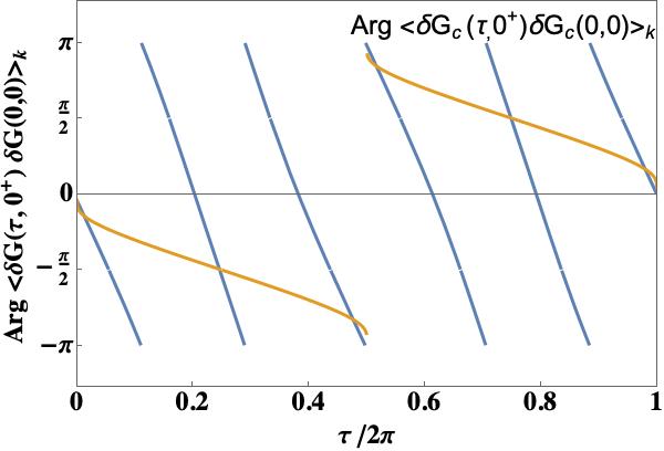
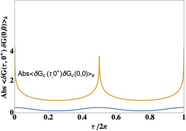
-55pt+55pt

Figure 2: The modulus and the phase of $\langle\delta G(\tau,0^{+})\delta G(0,0)\rangle_{k}$ (blue curves), obtained in Eq.(35), by averaging with the density matrix of Eq.(32), are plotted vs the dimensionless intradot imaginary time $\tau_{12}-\tau_{34}\equiv\tau$, in comparison with the naked one from Eq.(14) (orange curves). The prefactor $k^{2}{\tilde{a}}^{2}\>\beta t_{0}^{2}/(2\pi{\cal{J}})$, which contains the $k$ dependence, has been dropped in the plots.

Integrating out $\delta g_{\tau_{12},\tau_{+}},\delta g^{*}_{\tau_{12},\tau_{+}}$, the generating functional of the $\delta g$ fluctuations reads:

$${\cal{Z}}\left[\partial_{\tau}\varphi_{p}(\tau_{+})\right]=e^{-\frac{N}{2}\left\langle-i\>\partial_{\tau}\varphi_{p}\left|\left({\cal{F}}+\>\ \frac{t_{0}^{2}}{N}{p^{2}}R_{c}^{-1}\Lambda_{c}R_{c}^{-1}\right)\right|-i\>\partial_{\tau}\varphi_{p}\right\rangle}$$

(17)

where

$${\cal{F}}\left(\tau_{1},\tau_{2},\tau_{3},\tau_{4}\right)={R}_{c}^{-1}\>K_{c}\left[1-K_{c}\right]^{-1}{R}_{c}^{-1}$$ (18)

is the four point function of the $0+1$$-d$ SYK model. Integration over intermediate times is intended. Hereord ${\cal{F}}$ is ${\cal{O}}(1)$, with the meaning of ${\cal{O}}\left(\left[\frac{\beta{\cal{J}}}{N}\right]^{0}\right)$. As $R_{c}^{-1}\Lambda_{c}R_{c}^{-1}\propto G_{c}G_{c}$ is ${\cal{O}}(N/\beta{\cal{J}})$, it appears from Eq.(17) that we can define a physical parameter $\beta t_{0}^{2}/N{\cal{J}}$ of ${\cal{O}}(1)$, to guarantee that the hopping across the lattice is not irrelevant in the scaling. It turns out however that both ${\cal{F}}$ and $\frac{\beta t_{0}^{2}}{N{\cal{J}}}$ become of ${\cal{O}}\left(\frac{\beta{\cal{J}}}{N}\right)$ when the UV correction is included, which is crucially important to give sense to the functional integration of Eq.(15), as we explain here below.

Actually, the functional integral of Eq.(15) includes a divergent contribution due to the Goldstone modes $\delta g_{c}$ corresponding to eigenvalues of $K_{c}\to 1$, which has to be regularized resorting to the first UV correction $\langle\delta g|K_{c}^{-1}-1|\delta g\rangle\sim\beta{\cal{J}}$. The Faddeev Popov regularization provides an integration performed in the orthogonal space with respect to the $pGm$, while the smallest eigenvalue of the kernel $1-K_{c}$ is approximated with its UV correction, given by $1-k_{c}(h=2,n)\approx\frac{\alpha_{K}}{\beta{\cal{J}}}|n|+...$ ($\alpha_{K}\approx 3$ is a constant)Maldacena and Stanford (2016). It follows that the large, but finite contribution to ${\cal{F}}$ in Eq.(18) with this UV correction (i.e. for $\tau\sim 1/{\cal{J}}$) is not ${\cal{O}}(1)$ as stated here above, but ${\cal{O}}\left(\frac{\beta{\cal{J}}}{N}\right)$ and the same has to occur for $\frac{\beta t_{0}^{2}}{N{\cal{J}}}$. We will discuss this point in the next Section. The temperature threshold for coherence defined here, $T_{coh}=\frac{t_{0}^{2}}{N{\cal{J}}}$, is recurrent in the next.

If we ignore this matter for the time being, the generating functional of Eq.(17) provides the correlator $\frac{1}{N}FT\left[\delta g_{x}(\tau_{12},\tau_{+})\delta g_{x^{\prime}}(\tau_{34},0)\right]|_{k\neq 0}$ in imaginary time, inclusive of the hopping in the lattice:

$$\frac{\delta^{2}}{\delta\partial_{\tau}\varphi_{p}(\tau_{+})\>\delta\partial_{\tau}\varphi_{p}(\tau_{+}^{\prime})}\frac{1}{N}\sum_{p^{\prime}}\ln{{\cal{Z}}\left[\partial_{\tau}\varphi_{p^{\prime}}(\tau_{+})\right]}$$

$$\propto\frac{1}{2}\left(1+\>\frac{t_{0}^{2}}{2\>N}{p^{2}}R_{c}^{-1}\Lambda_{c}R_{c}^{-1}{\cal{F}}^{-1}\right){\cal{F}}.$$ (19)

This result adds to the naked correlator ${\cal{F}}$ the contribution coming from Eq.(13), so that the two dynamics are just added together in this approximation. However, one can envisage the present one as the lowest order of a ladder resummation which will appear more clearly in the next Section. The operator $\widehat{G_{c}G_{c}}\hat{{\cal{F}}}^{-1}$ appearing in the Kernel of Eq.(19) is the inverse matrix of Maldacena and Stanford (2016)

$${\cal{F}}\{G_{c}G_{c}\}^{-1}=\frac{6\alpha_{0}\beta{\cal{J}}}{\pi^{2}\alpha_{K}}\!\!\!$$

$$\times\sum_{|n|\geq 2,even}\!\!\!\!\!\frac{e^{i\>n(y_{12}-y_{34})}}{n^{2}(n^{2}-1)}\>f_{n}(\tau_{12})f_{n}(\tau_{34}),$$ (20)

where $y_{ij}\equiv(\tau_{i}+\tau_{j})/2$ in unit of $\hbar\beta/2\pi$. The basis functions $f_{n}(\tau_{12})$ are defined in appendix B, together with the spectral representation of the kernel $K_{c}^{-1}\>[1-K_{c}]$, as well as with their Fourier transform.

IV dressed correlator of ${pGm}$ modes

The derivation of the previous Section has assumed that $\varphi_{x}(\tau_{+})$ is given as an external source. However, continuation to real time requires that $\varphi_{x}(\tau_{+})$ acquires a dynamics. Meanwhile, the symmetry breaking induced by the UV perturbation source $\sim\partial_{\tau}$, couples to $G_{IR}$. $G_{IR}$ is derived from a time reparametrization under the diffeomorphism $e^{i\vartheta}\to e^{i\>\varphi_{x}(\vartheta)}$ of the conformal Green’s function ($\Delta=\frac{1}{4}$):

$$G_{IR}(\vartheta_{1},\vartheta_{2})=G_{c}\left(\!\varphi_{x}(\vartheta_{1}),\varphi_{x}(\vartheta_{2})\right)\!\varphi_{x}^{\prime}(\vartheta_{1})^{\Delta}\!\varphi_{x}^{\prime}(\vartheta_{2})^{\Delta},$$ (21)

where $\vartheta=2\pi\tau/\beta$ and $\varphi^{\prime}\equiv\partial_{\vartheta}\varphi$.

The leading correction to the conformal action arising from this reparametrization (apart for a shift of the ground state energy) is the SchwarzianKitaev :

$$\frac{I_{local}}{N}[\partial_{\tau}\varphi]=-2\pi\>\alpha_{S}\varepsilon\>\int\frac{d\vartheta}{2\pi}\left[\frac{1}{2}-\frac{(\varphi^{\prime\prime})^{2}-(\varphi^{\prime})^{2}}{2}\right].$$ (22)

Here $\alpha_{S}$ is a constantMaldacena and Stanford (2016) and $\varepsilon=1/\beta{\cal{J}}$. Hence, the full action in place of the one appearing in Eq.(17) reads:

$$I_{\partial\varphi}=\sum_{p}\left\{I_{local}[\partial_{\tau}\varphi_{p}]-\frac{N}{2}\int d\tau_{12}\left\langle-i\>\partial_{\tau}\varphi_{p}\left|\left({\cal{F}}+\>\ \frac{t_{0}^{2}}{N}{p^{2}}R_{c}^{-1}\Lambda_{c}R_{c}^{-1}\right)\right|-i\>\partial_{\tau}\varphi_{p}\right\rangle\right\}.$$ (23)

Now the field $\partial_{\tau}\varphi_{x}$ has its own dynamics and could be integrated out, possibly after adding a source term to get a generating functional of $\langle\partial\varphi\partial\varphi\rangle$ correlators. However, the action of Eq.(23) is essentially a "phase only" model for hopping of $\partial_{\tau}\varphi_{x}$ across the lattice. This is so, because we have neglected $\delta G\!\left(x,\tau_{12},\tau_{+}\right)$ appearing in Eq.(9). So as it stands, $I_{local}[\partial_{\tau}\varphi_{p}]\sim{\cal{O}}(N/\beta{\cal{J}})$, while the other term is ${\cal{O}}(1)$. Hence, the local action $I_{local}[\partial_{\tau}\varphi_{p}]$ is irrelevant in the $\beta{\cal{J}}\to\infty$ limit and the phase lacks its own dynamics. Writing down a partition function for the order parameter given by Eq.(9),with inclusion of its modulus, gives the chance of extracting correlation functions with include the UV correction and can be extended to real time. Let us denote the complex order parameter in two space dimension $\phi(x,\tau_{12},\tau_{+})=\sqrt{\rho_{0}+\delta\rho}\>e^{i\theta}$, for each degree of freedom. The functional integral, with $\tau$ of the dimension $time$ in the following, reads:

$$\int D\phi(x,\tau_{12},\tau_{+})^{*}D\phi(x,\tau_{12},\tau_{+})\>e^{-\tilde{S}\left[\phi^{*},\phi\right]}.$$ (24)

The action leading to the one of Eq.(23) can involve also space derivatives:

$$\tilde{S}=-\int^{\beta}\!\!\!\!d\tau_{12}\>\!\!\int\!d^{2}x\!\!\int^{\beta}\!\!\!\!d\tau\>\frac{1}{2}\left[-v^{2}\partial_{x}\partial_{\tau}\phi^{*}\partial_{x}\partial_{\tau}\phi\!+\!\left(\phi^{*}\partial_{\tau}\phi-\phi\partial_{\tau}\phi^{*}\right)\!-\!\frac{1}{2\pi\alpha_{S}\epsilon}\"{\i}\textquestiondown\textonehalf|\phi|^{4}\right]$$ (25)

(an expression for the velocity $v$ appearing here, derived from a Hamiltonian approach, is presented in Eq.(40) of the next Section and in the appendix D). In fact, expanding to quadratic order in $\theta$ and $\delta\rho$, we get (we imply $\int^{\beta}d\tau_{12}$ in the notation in what follows)

$$\tilde{S}_{2}=-\int d^{2}x\>\int^{\beta}d\tau\frac{1}{2}\left[-\rho_{0}v^{2}(\partial_{x}\partial_{\tau}\theta)^{2}\right.$$

$$\left.+2i\>\delta\rho\>\partial_{\tau}\theta-\frac{1}{2\pi\alpha_{S}\epsilon}\"{\i}\textquestiondown\textonehalf\delta\rho^{2}\right].$$ (26)

Integrating out the fast field $\delta\rho$ in the functional integral,

$$\int D\delta\rho\>e^{\int d^{2}x\>\int^{\beta}d\tau\left[i\>\delta\rho\>\partial_{\tau}\theta-\frac{1}{2\pi\alpha_{S}\epsilon}\"{\i}\textquestiondown\textonehalf\delta\rho^{2}\right]}$$

$$=e^{-\pi\alpha_{S}\epsilon\int d^{2}x\>\int^{\beta}d\tau\>\frac{1}{2}(\partial_{\tau}\theta)^{2}},$$ (27)

we obtain

$$\tilde{S}_{2}=-\int\!\!d^{2}x\!\!\int^{\beta}\!\!\!\!\!d\tau\!\!\left[-\rho_{0}\frac{v^{2}}{2}(\partial_{x}\partial_{\tau}\theta)^{2}+\pi\alpha_{S}\epsilon\frac{1}{2}(\partial_{\tau}\theta)^{2}\right],$$

(28)

which can be identified with $\frac{I_{local}}{N}\"{\i}\textquestiondown\textonehalf[\partial_{\tau}\varphi]$ of Eq.(22) provided we also introduce space non locality there, by trading $\frac{G_{c}(\tau_{12})}{\tilde{a}}v\>\partial_{x}$, which appears in Eq.(28), for $\partial_{\tau}$. Identification requires that

$$\rho_{0}=|\phi_{0}|^{2}=\frac{\pi\alpha_{S}\varepsilon}{\tilde{a}^{2}}\left|G_{c}(\tau_{12})\right|^{2},\>\>\>\>\>\partial_{\tau}\theta\equiv\partial_{\tau}\varphi$$ (29)

(an extra factor $N$ pops up from the number of flavours in the first equality). Introducing $\tilde{R}_{c}=\left|G_{c}(\tau_{12})\right|$ and substituting $-i\>\partial_{\tau}\varphi_{p}\to\>e^{-i\theta}\partial_{\tau}\phi_{p}\tilde{R}_{c}^{-1}\left[\frac{\pi\alpha_{S}\varepsilon}{\tilde{a}^{2}}\right]^{-1/2}$, the functional integral becomes

$$\int D\phi(x,\tau_{12},\tau_{+})^{*}D\phi(x,\tau_{12},\tau_{+})\>e^{-\tilde{S}\left[\phi^{*},\phi\right]}\>e^{-\frac{1}{2\pi\>\alpha_{S}\varepsilon}\sum_{p}\left\langle\phi_{p}\tilde{R}_{c}^{-1}\left|\overset{\rightarrow}{\partial_{\tau}}\left({\cal{F}}+\>\ \frac{t_{0}^{2}}{N}{p^{2}}R_{c}^{-1}\Lambda_{c}R_{c}^{-1}\right)\overset{\leftarrow}{\partial_{\tau}}\right|\phi_{p}\tilde{R}_{c}^{-1}\right\rangle},$$ (30)

where $\tilde{S}$ is given by Eq.(25). It is useful to ridefine the $\tilde{\phi}=\phi\>\tilde{R}_{c}^{-1}$ in the functional integral. In the change of the integration field, the action $\tilde{S}\left[\phi^{*},\phi\right]\to\tilde{S}\left[\tilde{\phi}^{*},\tilde{\phi}\right]$ acquires a factor $\left(G_{c}(\tau_{12})\right)^{2}$, except for the $|\phi|^{4}$ term which acquires the fourth power. Note, however, that in the UV domain is $\tau_{12}\sim{\cal{J}}^{-1}$, so that, withMaldacena and Stanford (2016) $b^{-2}=\sqrt{4\pi}{\cal{J}}$,

$$\left(G_{c}(\tau_{12})\right)^{2}=\frac{b^{2}}{|\tau_{12}|}\sim{\cal{O}}(1).$$ (31)

Hence, the last term of the full action from Eq.(30) is ${\cal{O}}(\beta{\cal{J}})$ in the large $\beta{\cal{J}}$ limit, while the first contribution to the full action, given by $\tilde{S}$, is ${\cal{O}}(1)$. Actually the $|\phi|^{4}$ term in $\tilde{S}$ is also ${\cal{O}}(\beta{\cal{J}})$, but we stick to zero order in the anharmonic functional integration. The evolution of Eq.(30) is characterized by an interplay between the dynamics of the intradot fluctuations and the dynamics of the interdot $\partial_{\tau}\varphi_{p}$ fluctuations, which is mostly represented by the action $\tilde{S}$. If $\tilde{S}$ is dropped alltogether, because it becomes irrelevant in the scaling, the gaussian integration of Eq.(30) can be easily performed, giving rise to a density matrix ${{\rho}}_{\delta g}$ of the intradot fluctuations at each given time $\tau_{+}$. When Fourier transformed with respect to the intradot times $\tau_{12},\tau_{34}$, stripping off the unperturbed evolution $\hat{{\cal{F}}}$, the result of the functional integration of Eq.(30), in the absence of $\tilde{S}$ is (again, $y_{ij}$ are center-of-mass times in unit of $\hbar\beta/2\pi$ and here $\tau\equiv\tau_{+}=y_{12}-y_{34}$ in unit of $\hbar\beta/2\pi$):

$${{\rho}}_{\delta g}\left(y_{12}-y_{34};p\right)_{m,m^{\prime}}\>\>\>\>\>\>\>\>\>\>\>\>$$

$$\sim\frac{1}{N}\left.\left\{1+\>\ \frac{t_{0}^{2}}{N}\frac{{p^{2}}}{2}\overset{\rightarrow}{\partial_{\tau}}\!\left(\left[\widehat{R_{c}^{-1}\Lambda_{c}R_{c}^{-1}}\right]\hat{{\cal{F}}}^{-1}\right)\!\overset{\leftarrow}{\partial_{\tau}}\right\}^{-1}\right|_{\tau_{+},m,m^{\prime}}\!\!\!\!\!\!\!\!\!\!\!\!\!\!\!\!\!\!.$$ (32)

We define

$$\hat{{\cal{B}}}_{m,m^{\prime}}(\tau_{+})\equiv\left[\overset{\rightarrow}{\partial_{\tau}}\!\left(\left[\widehat{R_{c}^{-1}\Lambda_{c}R_{c}^{-1}}\right]\hat{{\cal{F}}}^{-1}\right)\!\overset{\leftarrow}{\,}{\partial_{\tau}}\right]_{m,m^{\prime}},$$ (33)

which will be used in the following.

The correlation function $\left.\langle FT\left[\delta G_{x}(\tau_{12},\tau_{+})\delta G_{x^{\prime}}(\tau_{34},0)\right]\rangle\right|_{k\neq 0}$, corresponding to Eq.(13), but including the ladder resummation, is obtained by tracing on the density matrix of Eq.(32), after the $p=0$ term has been subtracted. To lowest order, we get:

$$\left.\langle FT\left[\delta G_{x}(0^{+},\tau_{+})\delta G_{x^{\prime}}(0,0)\right]\rangle\right|_{k\neq 0}$$

$$\approx\sum_{mm^{\prime}}G_{c}(\omega_{m})\>{{\rho}}_{\delta g}\!\left(\tau_{+};k\right)_{m,m^{\prime}}\>G_{c}(\omega_{m^{\prime}}).$$ (34)

where $G_{c}(\omega_{m})$ is given by Eq.(8). When $k\tilde{a}<<1$, the contribution of the ladder can be dropped and the unnormalized correlator $\langle\delta G(\tau_{12},\tau_{+})\delta G(\tau_{34},0)\rangle_{k\neq 0}$ reads:

$$\langle\delta G(\tau_{12},\tau_{+})\delta G(\tau_{34},0)\rangle_{k\neq 0}$$

$$\equiv FT_{k\neq 0}\langle\left[\delta G_{x}(\tau_{12},\tau_{+})\delta G_{x^{\prime}}(\tau_{34},0)\right]\rangle$$

$$=\frac{1}{N}\sum_{m}\frac{t_{0}^{2}}{2\>N}\>k^{2}\tilde{a}^{2}\left[\widehat{G_{c}{\cal{B}}G_{c}}\right]_{y,m,-m}\!\!\!e^{i\>\omega_{m}(\tau_{12}-\tau_{34})}.$$ (35)

Only the dependence on the relative coordinate $\tau_{12}-\tau_{34}\>\>mod.\>2\pi$ has been retained.

In Fig.2, the correlator $\langle\delta G(\tau,0^{+})\delta G(0,0)\rangle_{k}$ from Eq.(35) is plotted and compared with the naked $\langle\delta G_{c}\delta G_{c}\rangle_{k}$ correlator given by Eq.(14). The main panel of Fig.2 displays the modulus while the phase appears in the inset of Fig.2. The prefactor $k^{2}{\tilde{a}}^{2}\>\beta t_{0}^{2}/(2\pi{\cal{J}})$ has been dropped.

The correlator $\langle\delta G(\tau,0^{+})\delta G(0,0)\rangle_{k}$ has been calculated as reported in appendix B, using the Fourier Transform of Eq.20, with the inclusion of ${\cal{F}}^{-1}$ in the evolution. We had to truncate the sum over the (even) indices $n$ up to $n=12$, and consequently the sum over internal (odd) indices just includes up to $m,m^{\prime}=5$. Its modulus and phase, compared to those of the corresponding naked $\langle\delta G_{c}\delta G_{c}\rangle_{k}$ correlator, are plotted in Fig.2. The modulus of the naked correlator is exponentially decaying at the intradot time $\tau\sim 0,\>mod[2\pi]$, while the dressed one is powerlaw, highlighting the criticality of the phase, when the UV correction is included. The Fourier transform of the sawtooth phase oscillations of $\langle\delta G\delta G\rangle_{k}$ (blue curves) appearing in Fig.2 is not simply $\propto 1/i\>\omega_{m}$, revealing the "fast" intradot time scale induced by the UV correction, with respect to the phase of the naked correlator. They could have acquired further structure, if larger $n,m$ values had been retained.

The real part of the analytic continuation to real times of the center of mass coordinate $t_{+}$ in $\langle\delta G(0^{+},\tau_{+})\delta G(0,0)\rangle_{k}$ is plotted in the main panel of Fig.3 and compared to the corresponding naked correlation of Eq.(14). The same correlators, but keeping the dependence on the relative imaginary time coordinate $\tau_{12}-\tau_{34},\>\>mod[2\pi]$ as in Eq.(35), are plotted for various values of $\tau=\tau_{12}-\tau_{34}\>$ in the inset panel. The dependence on $\tau$ is oscillating and we have chosen values for $\tau$ within a single oscillation. The prefactor $k^{2}{\tilde{a}}^{2}\>\beta t_{0}^{2}/(2\pi{\cal{J}})$ has been dropped again. The $\langle\delta G(0^{+},\tau_{+})\delta G(0,0)\rangle_{k}$’s appearing in Fig.3 are scaled by $\times 10$ with respect to the correlators arising from the naked kinetic term of Eq.(14). The $t_{+}$ dependence in the presence of UV corrections appears very localized and highly variable with the intradot time, as compared with the naked one. The UV corrections squeeze the interdot correlations in time, increasing their "local" nature. This drastic drop in time of the correlations cannot guarantee quantum diffusion on an extended spae scale, much larger than the lattice spacing, and we have to resort to a better approximation which retains the dynamics entailed by the action $\tilde{S}$, which was lost in this result.

Besides, the strong dependence of the dressed correlations on the intradot imaginary time, with a relatively stable interdot real time dependence, confirms that the UV correction introduces a sizeable time scale separation between the intradot and interdot correlations. This is the basis of the factorization of the two dynamics, which we use to approximate the quantum diffusion discussed in the next Section.

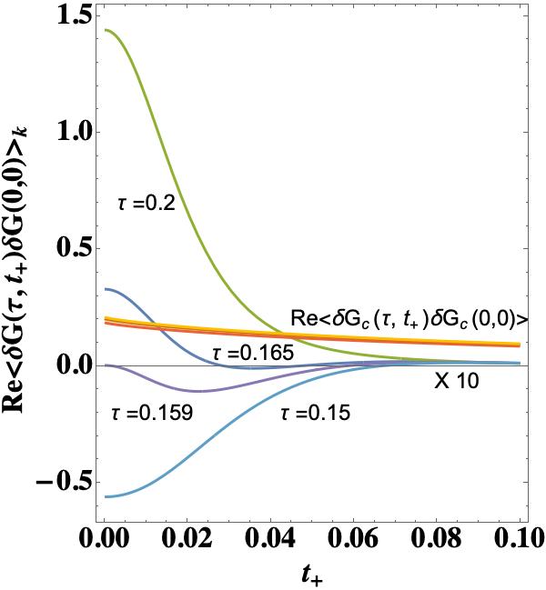
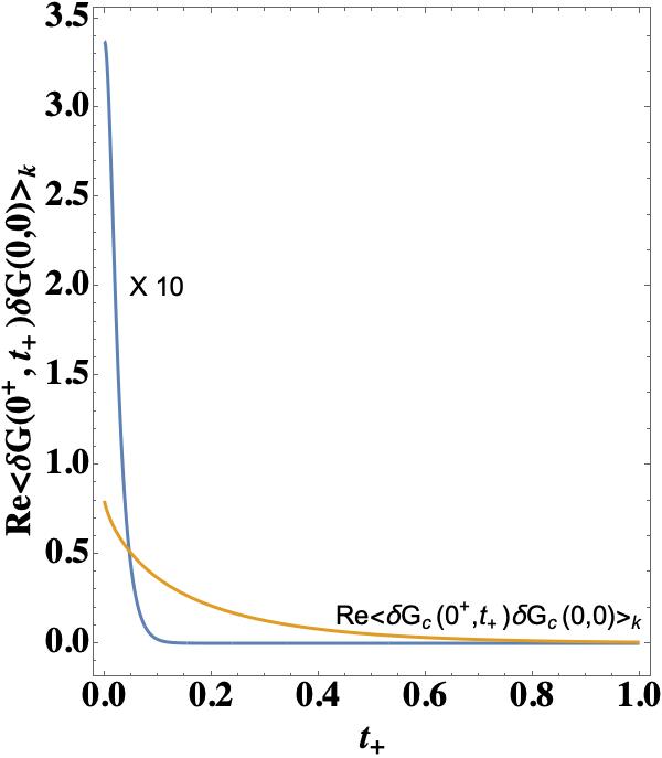
-22pt+60pt

Figure 3: The real part of the analytic continuation to real time of the correlator, $\Re e\langle\delta G(0^{+},t_{+})\delta G(0,0)\rangle_{k}$, given by Eq.(34) (blue curves), compared with the the naked correlator $\Re e\langle\delta G_{c}(\tau,t_{+})\delta G_{c}(0,0)\rangle_{k}$ from Eq.(14)(orange curves), are plotted vs the dimensionless interdot time $t_{+}$. While the intradot time $\tau_{12}-\tau_{34}\equiv\tau=0^{+}$ appears in the main panel, the curves for $\tau=0.15,0.159,0.165,0.2$ are plotted in the inset in an expanded scale. The oscillations of $\Re e\langle\delta G(\tau,t_{+})\delta G(0,0)\rangle_{k}$ in $\tau$ follow those appearing in Fig.2, while the naked correlator $\langle\delta G_{c}(\tau,t_{+})\delta G_{c}(0,0)\rangle_{k}$ has negligible dependence on $\tau$. The prefactor $k^{2}{\tilde{a}}^{2}\>\beta t_{0}^{2}/(2\pi{\cal{J}})$, which contains the $k$ dependence, has been dropped in the plots.

V quantum diffusion

In this Section, we attempt a better approximation for evaluating the partition function of Eq.(30), to investigate the quantum diffusion of the Q-excitations across the lattice, induced by the intradot $pGm$’s. We want to extract a diffusion coefficient $\tilde{D}_{Q}$ out of the scaling flow, to be related to the thermal conductance $\kappa$ of the "electronic" carriers and to the thermal "electronic" capacitance $C$ in the lattice. In turn, they are connected to a relaxation time ${\cal{T}}_{Q}$ and to the inverse lifetime of the Q-excitations, $\Gamma$.

V.1 Partition function of the Q-excitations

In Section IV we have shown that, to improve the $t_{+}$-dependence of the correlator $\Re e\langle\delta G(\tau,t_{+})\delta G(0,0)\rangle_{k}$ of Eq.(34), the UV local time corrections should be included more carefully. In fact, the result of the previous Section is unsatisfactory, because, in the flowing to the fixed point of the partition function of Eq.(30), we had to drop the order parameter dynamics entailed by the action ${\tilde{S}}$ of Eq.(25). A semiclassical approach to the diffusion process can be still envisaged, however, in the results of the previous Section. When the trace over the intradot frequencies is performed, the density matrix of Eq.(32), appropriately continued to real time, ${{\rho}}_{\delta g}\left(y_{12}-y_{34};k\right)_{m,m^{\prime}}\to{\cal{P}}\!\left(r,r^{\prime},t_{+}\right)$, takes the form of a heat kernel $z(t)$, typical of a diffusion processAkkermans and Montambaux (2007), defined as the probability to return to the origin, integrated over the point of departure. From Eq.(32), in the $k\tilde{a}<<1$ limit, we have :

$$z(t_{+})=\frac{1}{N}\int_{\cal{A}}\left[{\cal{F}}\cdot{\cal{P}}\right]\!\left(r,r,t_{+}\right)\>d^{2}r$$

$$\propto\sum_{m}\sum_{p}\>e^{-\left.\frac{\beta t_{0}^{2}}{N}\frac{{p^{2}}}{\hbar}\hat{{\cal{B}}}(t_{+})\right|_{m,m}},$$ (36)

where we have restored the free intradot evolution.

Now that we know what the drawback is, we reconsider the UV correction to the action given by Eq.(22). Its variation with respect to $\varphi^{\prime}$ gives a simple equation of motion $\partial_{\tau}^{2}\varphi^{\prime}=-\varphi^{\prime}$. When derived from the action of Eq.(28), this motion equation is rewritten in the form of lattice space oscillations. In the following we quantize these space extended excitations by means of a phenomenological 2-d Lagrangian with canonical conjugate variables, introduced in appendix B:

$$\dot{\theta}=\left(\frac{\kappa C}{\hbar T}\right)^{1/2}\!\!\frac{J_{Q}{\cal{T}}_{Q}}{k_{B}},\>\>\nabla\theta=\left(\frac{\hbar}{\kappa C\>T}\right)^{1/2}\!\!\frac{\kappa}{T}\nabla T.$$ (37)

Here $J_{Q}$ is the thermal energy current density. The corresponding Lagrangian is

$${\cal{L}}=\frac{1}{2}\int d^{2}x\>\left[\frac{k_{B}}{T}\>\left(\frac{J_{Q}{\cal{T}}_{Q}}{k_{B}}\right)^{2}+\frac{\hbar}{\kappa C}\>\left(\frac{\kappa}{T}\nabla T\right)^{2}\right]$$

$$\equiv\frac{1}{2}\int d^{2}x\>\left[\frac{\hbar k_{B}}{\kappa C}\>\dot{\theta}^{2}+T\>(\nabla\theta)^{2}\right].$$ (38)

The terms in the square brackets have dimension ${\cal{E}}/\ell^{2}$ (${\cal{E}}\equiv\>energy,\>\ell\equiv\>length$).

This Lagrangian is of course conserving, but we have introduced the relaxation time ${\cal{T}}_{Q}$, so that we can reproduce a diffusive motion equation of the form $J_{Q}=-\kappa\>\nabla T$, if we approximate the time derivative of the energy current fluctuations $\dot{J}_{Q}\approx{J}_{Q}/{\cal{T}}_{Q}$. Here $\kappa=\frac{C\>v\>\ell}{\tilde{a}_{\ell}^{2}}$ is the thermal conductivity in $2-d$, where $\ell$ and $v$ are typical mean free path and velocity, respectively, while $\tilde{a}_{\ell}^{2}\sim\tilde{D}_{Q}{\cal{T}}_{Q}$ is the area over which the thermal capacitance $C$ is defined and will be introduced here below.

We quantize the corresponding Hamiltonian, in terms of the creation and destruction bosonic operators ${a}^{\dagger}_{k},{a}_{k}$:

$$\pi_{k}=-i\>T^{1/2}\frac{1}{(2\Omega_{k})^{1/2}}|k|\>\left(a_{-k}-{a}^{\dagger}_{k}\right),$$

$$\theta_{k}=T^{-1/2}\frac{(2\Omega_{k})^{1/2}}{|k|}\>\left(a_{k}+{a}^{\dagger}_{-k}\right)$$

$$\Omega_{k}=\tilde{a}\left[\frac{\kappa}{k_{B}}\frac{CT}{\hbar}\right]^{1/2}|k|\equiv v\>|k|,$$ (39)

$${H}_{0}^{\tilde{D}}=\sum_{k}\Omega_{k}\>{a}^{\dagger}_{k}a_{k}+cnst.$$ (40)

$\Omega_{k}$ is the linear dispersion law of these modes with velocity $v$ defined in Eq.(39). From the damped fluctuations of these modes, the response function $D^{\beta}(\omega)$ is derived in eq (179), within this Lagrangian approach. On the contrary, here in the following, we aim to deriving the quantum diffusion probability, stressing the interplay between intradot $\delta g_{m}$ modes and the kinetics of the Q-fluctuations in the lattice.

From Eq.(30), we recognize the coupling Hamiltonian $\hat{{\cal{H}}}_{\tilde{D}}$, which, in the interaction representation of $\hat{H}_{0}^{\tilde{D}}$, takes the form:

$$\hat{{\cal{H}}}_{\tilde{D}}(\tau)=-\frac{\tilde{a}^{2}}{\pi\alpha_{S}N\varepsilon}\sum_{p\neq 0}{p^{2}}\>\frac{\beta t_{0}^{2}}{2N}\times\>\>\>\>$$ (41)

$$\sum_{k}\!\hat{{\cal{B}}}(\tau)\>{a}^{\dagger}_{k+p}(\tau){a}_{k}(\tau).$$

$\hat{{\cal{H}}}_{\tilde{D}}(\tau_{+})$ of Eq.(41) represents an "effective interaction Hamiltonian" for energies in the incoherent phase. We remind that $\hat{{\cal{B}}}(\tau)$, defined in Eq.(33), is $\sim{\cal{O}}\left(\frac{N}{\beta{\cal{J}}}\right)$ and that the $hat$ denotes the $m\times m^{\prime}$ matrix structure. As $\frac{\beta t_{0}^{2}}{2N}\sim{\cal{O}}\left(\frac{\beta{\cal{J}}}{N}\right)$, the additional factor $(\pi\alpha_{s}N\epsilon)^{-1}$ in Eq.(41) makes ord $\hat{{\cal{H}}}_{\tilde{D}}$ of ${\cal{O}}\left(\frac{\beta{\cal{J}}}{N}\right)$ and allows us to define a scaled length $\tilde{a}_{\ell}\sim\tilde{a}\>(\pi\alpha_{s}N\epsilon)^{-1/2}>>\tilde{a}$, which is the length scale for diffusion in the lattice.

The partition function of Eq.(30), represented in the bosonic coherent field $\tilde{\phi}=\phi R_{c}^{-1}$, can be expressed as

$${\bf Tr}\>e^{-\beta H^{0}_{SYK}}\!\!\left\{\!{\large\bf tr_{\tilde{\phi}}}\!\!\left(e^{-\beta H_{0}^{\tilde{D}}}\!{\bf T_{\tau_{+}}}\!\!\left[e^{-\int_{0}^{\beta}\hat{{\cal{H}}}_{\tilde{D}}(\tilde{\phi}^{*},\tilde{\phi},\tau_{+})\>d\tau_{+}}\right]\!\right)\!\right\}$$

(42)

and the full quantum dynamics, is included (we drop the tilde on $\phi$ henceforth). Here ${\bf tr_{\phi}}$ denotes the trace of a time ordered functional integral (${\bf T_{\tau_{+}}}$ is time ordering in $\tau_{+}$), while we keep the symbol ${\bf Tr}$ for the trace of the $m\times m$ matrices. $\hat{{\cal{H}}}_{\tilde{D}}(\phi^{*},\phi,\tau_{+})$ is the matrix element derived from Eq.(41), in the coherent basis representation. In performing the trace, we assume $\hat{{\cal{H}}}_{\tilde{D}}\!(\phi_{p}^{*},\phi_{p},\tau)$ to be diagonal in the $p$ label.

As we are dropping the $|\phi|^{4}$ term appearing in the original action $\tilde{S}$ of Eq.(30), our toy model involves non interacting bosonic fields only. The partition function can be written down straightforwardly by slicing the trace ${\bf tr_{\tilde{\phi}}}$ into $\frac{\beta}{M}$ time slices ($M$ integer)Negele and Orland (1987):

$${\cal{Z}}=\lim_{M\to\infty}{\bf Tr}\left\{e^{-\beta H^{0}_{SYK}}\right.$$

$$\times\left.\prod_{k}\left[1-\left\{e^{\frac{\beta}{M}k^{2}\frac{\tilde{a}^{2}}{\pi\alpha_{S}N\epsilon}\frac{\beta t_{0}^{2}}{N}\>\hat{{\cal{B}}}\left(\frac{\beta}{M}\right)}\right\}^{M}\right]^{-1}\right\}.$$ (43)

In Eq.(43) the dynamics of the intradot fluctuations $\delta g_{m}$ and their interdot extension to the lattice are fully entangled. In view of some simplification, we limit ourselves to the regime in which the inverse timescale of the Q-fluctuations in the lattice, $\overline{\tau}^{-1}\equiv-i\>{\cal{T}}_{Q}^{-1}$, is much smaller than the typical frequency scale of the intradot evolution (which includes the dominant term of the UV corrections). In this regime we factorize the $\left(\frac{\beta}{M}\right)$ slices of the intradot propagator generated by $H^{0}_{SYK}$ which is $\hat{{\cal{F}}}$, while $\hat{{\cal{B}}}$ includes the kernel $\widehat{G_{c}G_{c}{\cal{F}}^{-1}}$ of the Q-fluctuations. The factorization amounts to a kind of "non interacting blip approximation"Chakravarty and Leggett (1984); Roman (1969) and can be justified as long as the thermalization is very effective.

With this approximation, the functional integration of the partition function of Eq.(43) can be cast in the form:

$$\lim_{M\to\infty}\prod_{k}\!{\bf Tr}\!\left\{\hat{{\cal{F}}}(\beta)\left[1\!-\!\left(1-\frac{\beta}{M}k_{B}T_{0}\hat{f}_{\overline{\tau}}(k)\right)^{M}\right]^{-1}\!\right\},\>\>\>\>$$ (44)

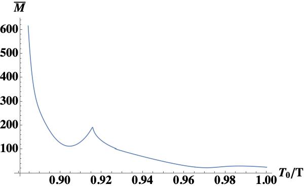
Figure 4: Plot of the approximate lowest $\overline{M}$ value which fulfills the unitarity condition of the partition function in Eq.(46), up to $10^{-5}$, vs. $T_{0}/T$ values, for $k\tilde{a}=1$.

where $\frac{\beta}{M}k_{B}T_{0}\>\hat{f}_{\overline{\tau}}\left(k\right)$ is a linearized $m\times m$ matrix, for a small increment $\frac{\beta}{M}$ of $\tau_{+}$, arising from the correspondence

$$-k^{2}\frac{\tilde{a}^{2}}{\pi\alpha_{S}N\epsilon}\frac{\beta t_{0}^{2}}{N}\>\hat{{\cal{B}}}\left(\frac{\beta}{M}\right)\to\frac{\beta}{M}k_{B}T_{0}\>{\hat{f}}_{\overline{\tau}}\!\left(k\right)\!.$$ (45)

The subscript $\overline{\tau}$ is to remind that the factorization of the traces is only justified in a limited temperature range in which the separation of the time scales holds. We have extracted a temperature scale $T_{0}$ from the left hand side, of ${\cal{O}}\!\left(\frac{\beta{\cal{J}}}{N}\right)$, and introduced the function $\hat{f}_{\overline{\tau}}$ of ${\cal{O}}\left(1\right)$.

As we are on a closed time contourKamenev and Levchenko (2009), the partition function should be unity. The intradot propagation should be periodic in $\tau_{+}$, as well: ${\bf Tr}\left\{\hat{{\cal{F}}}(\beta)\right\}=1$. As both $\hat{{\cal{F}}}(\beta)$ and ${\hat{f}}_{\overline{\tau}}$ in Eq.(44) are $m\times m$ matrix of rank $\tilde{r}_{m}$, the limit of the trace is costly from the numerical point of view. It can be done straightforwardly if we trade $1/\tilde{r}_{m}$ for the stripping of $\hat{{\cal{F}}}(\beta)$ off the trace. Once done this, we have checked what is the minimal $M$ value, $\overline{M}$, which fulfills unitarity, at a given approximation order:

$${\bf z}_{\overline{M}}\left(k\right)=\frac{1}{\tilde{r}_{m}}{\bf Tr}\left\{\frac{1}{\hat{1}-\frac{1}{\tilde{r}_{m}}\>\left(e^{-\frac{1}{\overline{M}}\frac{T_{0}}{T}{{\hat{f}}}_{\overline{\tau}}}\right)^{\overline{M}}}\right\}\approx 1.$$ (46)

In Fig.4, we plot an interpolated smoothed curve of the (approximate) lowest $\overline{M}$ value, which satisfies Eq.(46), vs. $T_{0}/T$, for $k^{2}\tilde{a}_{\ell}^{2}=1$. Precision is up to $>10^{-5}$. $\overline{M}$ is practically constant, when $\frac{T_{0}}{T}\gtrapprox 1$, but it increases strongly when $T$ takes values $T>T_{0}$. The trend is only meaningful for $T_{0}/T\sim 1$, because $T$ values larger than $T_{0}$ require $n>12$ in the spectral representation of Eq.(20) and matrices $m\times m$ of rank $\tilde{r}>3$, i.e. higher than the ones used here. Fig.4 is the numerical proof that $T_{0}$ represents the temperature above which the thermalization is more efficient and our factorization between evolutions breaks down. The threshold temperature scale $T_{0}$ introduced in Eq.(45) and the space scale $\tilde{a}_{\ell}$ defined after Eq.(41) are discussed in Subsection C.

V.2 $\langle\overline{\delta G^{R}\delta G^{A}}\rangle$ diffusion probability

The generating functional to obtain the correlator of the field $\phi_{p}(\tau)$ at different times $y^{r}-y^{s}$ ($y^{r}\equiv 2\pi r/\overline{M};\>r,s\>integers$) can be derived from Eq.(42) by adding a source term. Its ${r,s}$ matrix element can be denoted as ${\bf Tr}\left(\left[\partial_{\tau}+\hat{{\cal{H}}}_{\tilde{D}}\right]^{-1}\right)_{r,s}$:

$$\lim_{M\to\infty}{\bf Tr}\left(\left[\partial_{\tau}+\hat{{\cal{H}}}_{\tilde{D}}\right]^{-1}\right)_{r,s}\approx\lim_{M\to\infty}{\bf Tr}\left\{\left[\hat{{\cal{F}}}\left(\frac{\beta}{M}\right)\right]^{r-s}\frac{\left(1-\frac{1}{M}\ \frac{T_{0}}{T}\hat{f}_{\overline{\tau}}\right)^{(r-s)}}{1-\left[\hat{{\cal{F}}}\!\left(\frac{\beta}{M}\right)\left(1-\frac{1}{M}\frac{T_{0}}{T}\hat{f}_{\overline{\tau}}\right)^{M}\right]}\right\}$$

$$\approx\lim_{M\to\infty}{\bf Tr}\left\{\left[\hat{{\cal{F}}}\!\left(\frac{\beta}{M}\right)\right]^{r-s}\right\}\>{\bf Tr}\left\{\frac{\left[e^{-\frac{T_{0}}{T}\hat{f}_{\overline{\tau}}}\right]^{(y^{r}-y^{s})}}{\hat{1}-\frac{1}{\tilde{r}_{m}}\left[e^{-\frac{T_{0}}{T}\hat{f}_{\overline{\tau}}}\right]}\right\}\!\!\approx\lim_{M\to\infty}{\bf Tr}\left\{\left[\hat{{\cal{F}}}\!\left(\frac{\beta}{M}\right)\right]^{r-s}\right\}\>{\bf Tr}\left\{\left[e^{-\frac{T_{0}}{T}\hat{f}_{\overline{\tau}}}\right]^{(y^{r}-y^{s})}\right\},$$ (47)

to be compared with the correlators of Eq.(34) and Eq.(35) ( here the term $k=0$ has not been subtracted, yet).

According to Eq.(36), our aim is to define a scalar diffusion coefficient $\tilde{D}_{Q}$ such that, when moving from euclidean to real time, ${\bf Tr}\left[e^{-\frac{T_{0}}{T}\hat{f}_{\overline{\tau}}}\right]\to e^{-i\>\tilde{D}_{Q}\>k^{2}{\cal{T}}_{Q}}$. To accomplish this, we have to check that ${\bf Tr}\left[e^{-\frac{T_{0}}{\overline{M}T}\hat{f}_{\overline{\tau}}}\right]$ provides an exponential with a $k^{2}$ factor in the exponent, when the trace has been performed. In Fig.5, we plot , vs $(k\tilde{a}_{\ell})^{2}$, the logarithm of the last term of the propagator on the right hand side of Eq.(47) for $y^{r}-y^{s}=1$,

$$\ln\left({\bf Tr}\left[e^{-\frac{T_{0}}{\overline{M}T}\hat{f}_{\overline{\tau}}}\right]^{1}\right),$$ (48)

for $\frac{T_{0}}{\overline{M}T}=0.005,\>0.01,\>0.03$ and we see that it is a linear function of $(k\tilde{a}_{\ell})^{2}$, for $(k\tilde{a}_{\ell})^{2}>0.5$. The linear dependence confirms that, not only the single matrix element contributions of Eq.(45), but also the logarithm of the trace appearing in Eq.(48) has the linear dependence on $(k\tilde{a}_{\ell})^{2}$. This linear dependence on $(k\tilde{a}_{\ell})^{2}$ is the signature of the diffusivity of the Q-excitation modes which sets in at larger values of $(k\tilde{a}_{\ell})^{2}$. The scale $k\tilde{a}_{\ell}>1$ characterizes the virtual Q-fluctuations, which we are investigating, by including the UV corrections.

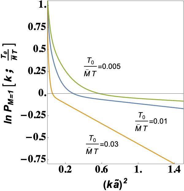
Figure 5: Plot of the logarithm of the propagator appearing in Eq.(48) for $y^{r}-y^{s}=1$ (i.e.. $M=1$) , $\ln\left({\bf Tr}\left[e^{-\frac{T_{0}}{\overline{M}T}\hat{f}_{\overline{\tau}}}\right]^{1}\right)$, vs $(k\tilde{a}_{\ell})^{2}$, for $\frac{T_{0}}{\overline{M}T}=0.005,\>0.01,\>0.03$, displaying an approximately linear behavior as a function of $(k\tilde{a})^{2}$, for $(k\tilde{a})^{2}>0.5$.

To sum up, the steps of the logical inference starting from Eq.(45) are

$$\left.-k^{2}\frac{\tilde{a}^{2}}{\pi\alpha_{S}N\epsilon}\frac{\beta t_{0}^{2}}{N}\>\hat{{\cal{B}}}\>\right|_{\tau_{+}=\beta/M}\to\frac{\beta}{M}k_{B}T_{0}\>{\hat{f}}_{\overline{\tau}}\!\left(k;\frac{\beta}{M}\right)$$

$$\to\ln\left({\bf Tr}\left[e^{-\frac{T_{0}}{\overline{M}T}\hat{f}_{\overline{\tau}}}\right]^{\frac{\beta}{M}=1}\right)\to\frac{T_{0}}{\overline{M}T}\>{\overline{f}}_{\overline{\tau}}\to\tilde{D}_{Q}\>k^{2}\frac{{\cal{T}}_{Q}}{\overline{M}}.$$ (49)

As the left hand side is ${\cal{O}}\left(\frac{\beta{\cal{J}}}{N}\right)$, the product $\tilde{D}_{Q}{\cal{T}}_{Q}$ is ${\cal{O}}\left(\frac{\beta{\cal{J}}}{N}\right)$, as well. In fact we will put $\tilde{D}_{Q}{\cal{T}}_{Q}=\tilde{a}_{\ell}^{2}=\tilde{a}^{2}T_{0}/T$. The diffusion coefficient $\tilde{D}_{Q}$ and the relaxation time scale of the diffusion process $i\>{\cal{T}}_{Q}\equiv\overline{\tau}$ are discussed in Subsection C.

Our simplified approach to the diffusive constant ${\tilde{D}}_{Q}$ provides an analytical approximate expression for $\langle\delta G(0^{+},\tau_{+})\delta G(0,0)\rangle_{k}$. From the left hand side of the second line of Eq.(47) we write:

$$\left.\langle\delta G(0^{+},y)\delta G(0,0)\rangle\right|_{k\neq 0}\propto\frac{e^{-{\overline{f}_{k}}^{\prime}\>y}}{1-e^{-2\pi\>{\overline{f}_{k}}^{\prime}}},$$ (50)

with ${\overline{f}_{k}}^{\prime}=\beta\tilde{D}_{Q}k^{2}/2\>\pi$. By Fourier transforming to Matsubara Bose frequencies ($n$ stands here for $\beta\Omega_{n}/2\>\pi$) we obtain:

$$\int_{0}^{2\pi}dy\frac{e^{-{\overline{f}_{k}}^{\prime}y}}{1-e^{-2\pi\>{\overline{f}_{k}}^{\prime}}}\>e^{i\>n\>y}=\frac{1-e^{-2\pi\>{\overline{f}_{k}}^{\prime}+2\pi\>i\>n}}{{\overline{f}_{k}}^{\prime}-i\>n}\frac{1}{1-e^{-2\pi\>{\overline{f}_{k}}^{\prime}}}$$

so that:

$$\left.\left\{\langle\delta G(0^{+},\tau_{+})\delta G(0,0)\rangle\right\}\right|_{k\neq 0,n}\propto\frac{2\pi}{\beta}\frac{1}{\tilde{D}_{Q}k^{2}-i\>\Omega_{n}}.$$ (51)

This result highlights the diffusive pole in the Fourier transform of the Q-fluctuation correlatorGu et al. (2017).

Identifications of the threshold temperature, $T_{0}$, and of the space parameters, $\tilde{a}_{\ell}$, $\tilde{D}_{Q}{\cal{T}}_{Q}$, introduced as scales in the previous derivation, require a modelization of the damped dynamics of the Q-excitations, which we derive in the next Subsection C. While these parameters, in the course of the derivation, have been recognized as marginal in a renormalization group sense, as they are ${\cal{O}}\left(\frac{\beta{\cal{J}}}{N}\right)$ (in the limit ${\cal{J}},N\to\infty$, ${\cal{J}}/N\to cnst$), they should rest on phenomenological fundamental quantities, like the thermal capacitance $C$ per unit mass and the thermal conductivity $\kappa$. These quantities will be related to two parameters, i.e. the damping of the neutral Q-excitations, $\Gamma$, and their propagation velocity $v$, given by Eq.(39) in our model. The velocity $v$, appears in the linear spectrum of the Q- excitations given by Eq.(40), while $\Gamma$ is introduced as a broadening of their spectral peak. Subsection C is devoted to the presentation and discussion of these relations.

V.3 Thermalized and coherent energy processes

In the previous Sections we have shown how the $pGm$ within each SYK dot, $\delta g_{m}$, generate energy modes diffusing in the lattice of the extended SYK model. The validity of our approach, involving the partial factorization that we have adopted in our traces, rests on different temporal dependence scales of the center of mass times $y^{r}-y^{s}$ on one side and of the intradot fluctuations on the other. The "interdot" dynamical time scale is discussed phenomenologically in this Subsection.

The "interdot" time scale is the thermalization time ${\cal{T}}_{Q}$, introduced in Eq.(49). ${\cal{T}}_{Q}$, the threshold temperature scale for thermalization $T_{0}$, and the space scale $\tilde{a}_{\ell}$, are connected with the velocity $v$, given by Eq.(39), and with the phenomenological damping $\Gamma$, which is the inverse lifetime of the Q-excitations. In turn, these quantities depend on the thermal capacitance $C$ per unit mass and the thermal conductivity $\kappa$, which are the phenomenological, experimentally measurable quantities.

When adopting our rough approximations, we cannot ignore that these parameters depend on temperature. In particular, the two sets of scales should be considered, $(T_{coh},{\cal{T}}_{Q})$ related to particle transport in the coherent phase and $\left(T_{0}\cdot\left(\frac{N}{\beta{\cal{J}}}\right),\hbar\beta\right)$ for a thermalized system in the incoherent phase, when $T\gtrsim T_{0}>T_{coh}$. The parameters $T_{coh},{\cal{T}}_{Q},T_{0}$ and $\tilde{a}_{\ell}^{2}$ are ${\cal{O}}\left(\frac{\beta{\cal{J}}}{N}\right)$. We will discuss the two regimes in this Subsection. At finite $T$ the small gap of the $Q-$excitations can be disregarded. We assume that both regimes have gapless and chargeless bosonic excitation modes of energy $\Omega_{k}=\hbar v|k|$, given by Eq.(39). Indeed, we exclude charging effects in transport. In the incoherent regime the gaussian action of Eq.(28) involves energy density ${\cal{N}}\propto\partial_{\tau}\theta$ fluctuations and energy flux density $\dot{{\cal{N}}}\propto J_{Q}$ fluctuationsDavison et al. (2017), the Q-excitations. In the coherent phase, bosonic excitations are particle-hole excitations with fluctuations of the particle number $N_{e}$ and first sound excitations. In the appendix E we show that the sound mode survives when the interaction with the SYK dots is turned on perturbatively, embedded in the p-h continuum. We attribute an inverse lifetime $\Gamma\propto T$ to these excitations.

We proceed with the incoherent regime first, at $T\approx T_{0}$. The thermal conductivity, in presence of a damping $\Gamma$, is derived in Eq. (181) from the $J_{Q}-J_{Q}$ response:

$$\kappa=k_{B}\>\Gamma\>\left(\frac{h\>\Gamma}{CT}\"{\i}\textquestiondown\textonehalf\right)^{1/2}.$$ (52)

From one of the Einstein relations, the diffusivity $\tilde{D}_{Q}$ is related to the thermal capacitance $C$ and to the density $\rho_{0}$, according to (p-h symmetry is assumed)

$$\tilde{D}_{Q}=\frac{\kappa}{C\rho_{0}}.$$ (53)

As the chemical potential $\mu$ is assumed to vanish, the 2-d particle density $\rho_{0}$ involved in these excitations, given by Eq.(29), is not well phenomenologically defined. We will estimate it as $\rho_{0}=\Gamma^{2}/v^{2}$, a choice that will turn out to be consistent with our results of this Subsection. We proceed now by deriving an estimate of $T_{0}$. In this case, energy diffusion is mainly due to heat transport in a highly thermalizable environment and we use the first temperature dependent correction to the energy of the SYK modelMaldacena and Stanford (2016): $\delta E=c/(2\beta^{2})=CT$ in Eq.(52), where $c=4\pi^{2}\alpha_{S}N/{\cal{J}}$. From Eq.(52), we get:

$$\kappa=k_{B}\>\Gamma^{3/2}\left(\hbar\beta\right)^{1/2}\>\left(\frac{\beta{\cal{J}}}{\pi\alpha_{S}N}\"{\i}\textquestiondown\textonehalf\right)^{1/2},$$ (54)

which, inserted in Eq.(53), with $\rho_{0}=\Gamma^{2}/v^{2}$ gives:

$$\tilde{D}_{Q}=\Gamma\left(\frac{\beta{\cal{J}}}{\pi\alpha_{S}N}\"{\i}\textquestiondown\textonehalf\right)\>\tilde{a}^{2},$$ (55)

where Eq.(39) has been used. On the other hand, the last inference in Eq.(49), together with Eq.(45), suggests that ${\overline{f}}_{\overline{\tau}}\propto k^{2}\tilde{a}^{2}$, with $\tilde{a}_{\ell}^{2}\sim\tilde{a}^{2}{T_{0}}/{T}$. We conclude from Eq.(55) that $\tilde{D}_{Q}\propto\Gamma\>\tilde{a}_{\ell}^{2}$ and, as $\tilde{D}_{Q}{\cal{T}}_{Q}=\tilde{a}^{2}_{\ell}$, the relaxation timeHartnoll (2015) ${\cal{T}}_{Q}\sim\Gamma^{-1}\sim\hbar\beta$. Thermalization is better handled in euclidean time. Putting ${\cal{T}}_{Q}\to\hbar\beta$ in $\tilde{a}^{2}\frac{T_{0}}{T}\sim\tilde{D}_{Q}{\cal{T}}_{Q}$ and using Eq.(55), we conclude that

$$k_{B}T_{0}\sim 2\pi\>\hbar\>\Gamma\left(\frac{\beta{\cal{J}}}{N\pi\alpha_{S}}\"{\i}\textquestiondown\textonehalf\right).$$ (56)

This equation qualifies $k_{B}T_{0}$ as a threshold energy for efficient thermalization and confirms that $T_{0}$ is ${\cal{O}}\!\left(\frac{\beta{\cal{J}}}{N\pi\alpha_{S}}\"{\i}\textquestiondown\textonehalf\right)$, if just the zero order for $\Gamma$ is retained. As we have assumed that $\Gamma\propto T$, both $\tilde{D}_{Q}$ of Eq.(55) and $T_{0}$ of Eq.(56) are temperature independent.

Our approximations, which involve some kind of adiabatic factorization, do not allow us to discuss the coherent carrier transport regime, $T\lesssim\Omega_{n}\ \lesssim T_{coh}<T_{0}$, except for a very qualitative bird’s eye. Indeed, the convergence of the ’normalization’ of Eq.(46) in Fig.4 is misleading, as one should keep in mind that just the dominant UV contribution of ${\cal{F}}$ has been retained and all the regular contributions (belonging to the fluctuation domain orthogonal to the $pGm$’s) have been neglected. These include low energy contributions and their evolution cannot be factorized. Anyhow, back to Eq.(53) for this case, an approximated expression for the specific heat arising from the gapless modes of the model given by Eq.s(39,40) is given by Eq (D):

$$C_{{\cal{V}}}=k_{B}\frac{1}{2\pi}\left(\frac{k_{B}T}{\hbar v}\right)^{2}\>6\>\zeta[3],$$ (57)

where $\zeta[n]$ is the Riemann function. When the velocity $v$ is inserted in this expression, we get an equation for $1/C_{{\cal{V}}}^{2}$, which can be related to Eq.(52) to give:

$$\left(\frac{\kappa}{k_{B}\Gamma}\right)^{4}\frac{1}{(h\Gamma)^{2}}\"{\i}\textquestiondown\textonehalf=\frac{1}{C_{{\cal{V}}}^{2}T^{2}}\"{\i}\textquestiondown\textonehalf=\frac{2\pi}{k_{B}}\>\frac{\hbar}{(k_{B}T)^{3}}\>\frac{\kappa}{6\>\zeta[3]}.$$ (58)

Inserting this result in Eq.(53), with $v$ given by Eq.(39) and $\rho_{0}=\Gamma^{2}/v^{2}$we obtain:

$$\tilde{D}_{Q}=\frac{\kappa^{2}}{\Gamma^{2}}\frac{T}{\hbar k_{B}}\tilde{a}^{2}=\frac{\hbar^{2}\Gamma^{2}}{\hbar}\frac{1}{k_{B}T}\left(\frac{1}{6\>\zeta[3]}\right)^{1/3}\tilde{a}^{2}.$$ (59)

Assuming again $\Gamma\sim T$, Eq.(59) shows that the diffusion constant is in this case $\propto T$ as in the Einstein -Smoluchowski formula. At least formally, it can be put in the form of a bound on the diffusion rate, which has been conjectured for strongly interacting systems at zero chemical potentialKovtun et al. (2005); Hartnoll (2015):

$$\tilde{D}_{Q}\gtrsim\hbar\frac{\Gamma^{2}\tilde{a}^{2}}{k_{B}T}.$$ (60)

In this case the velocity which arises here is not $v_{F}$ but $\tilde{v}\sim\tilde{a}\Gamma$. Eq.(60) is non universal.

Now we proceed just by analogy with the previous case and we assume that, just by replacing $T_{0}$ with $T_{coh}$, we can put here

$$\tilde{a}^{2}_{\ell}\sim\tilde{D}_{Q}{\cal{T}}_{Q}=\tilde{a}^{2}T_{coh}/T.$$ (61)

From Eq.(59) it follows that:

$$\tilde{a}^{2}\frac{T_{coh}}{T}\sim\frac{\hbar^{2}\Gamma^{2}}{\hbar}\frac{1}{k_{B}T}\left(\frac{1}{6\>\zeta[3]}\right)^{1/3}\tilde{a}^{2}{\cal{T}}_{Q}^{coh},$$ (62)

what implies:

$${\cal{T}}_{Q}^{coh}\sim\left(6\>\zeta[3]\right)^{1/3}\frac{k_{B}T_{coh}}{\hbar\Gamma^{2}}.$$ (63)

Given $T_{coh}\propto t_{0}^{2}/N{\cal{J}}\sim{\cal{J}}/N$ , is ${\cal{T}}_{Q}^{coh}\propto T^{-2}$ as in the Fermi liquid case.

VI superconductive coupling at low temperature

In this Section we present an Eliashberg approach to the superconducting instability of a quantum electron liquid that contains the Q-excitations in its energy spectrum. As explained in the Introduction, we consider a model with two components: a lattice of local $0+1-d$ SYK dots and an underlying FL which interacts with the dot lattice perturbatively. Higher dimensional complex SYK models with non-random intersite hopping have been constructed with fascinating NFL propertiesHaldar et al. (2018); Lantagne-Hurtubise et al. (2021). We use a perturbative approachChowdhury et al. (2018) in Subsection A and derive the selfenergy of the coherent phase of the quantum liquid, which turns out to be a MFL with short lived and ill defined quasiparticles. In Subsection B we assume an attractive pairing among the quasiparticles, mediated by the virtual Q-excitations, and we derive the critical temperature $T_{c}$, which is non BCS-like.

VI.1 Marginal Fermi liquid

The quasiparticles of a low energy $2-d$ FL have a quasiparticle residue $Z$ and a single particle energy $\epsilon_{\vec{k}}=\tilde{v_{F}}k$ in the continuum limit, with a renormalized physical velocity $v_{F}^{*}=Z\tilde{v}_{F}$ and a residual local interaction of strength $U_{c}$, which is dealt with perturbatively. The isotropic self-energy arising from the interaction, for $k$ on the Fermi surface, is:

$$\Sigma(k_{F},i\omega)\hskip 170.71652pt$$

$$=U_{c}\sum_{\vec{q}}\int\frac{d\Omega}{2\pi}\>G(\epsilon_{\vec{k}_{F}+\vec{q}}-\epsilon_{\vec{k}_{F}},i\omega+i\>\Omega)\>\Pi(q,i\>\Omega)$$

$$\approx U_{c}\sum_{\vec{q}}\int\frac{d\Omega}{2\pi}\>\frac{1}{iZ^{-1}(\omega+\Omega)-\tilde{v}_{F}q\cos\theta}\>\Pi(q,i\>\Omega).$$ (64)

In Eq.(64), $\theta$ is the angle between $\vec{q}$ and $\vec{k}=\vec{k}_{F}$ and, for $|q|<<k_{F}$, we have approximated $\epsilon_{\vec{k}_{F}-\vec{q}}-\epsilon_{\vec{k}_{F}}\approx\tilde{v}_{F}q\cos\theta$.

$\Pi(q,i\>\Omega)$ is the polarization function

$$\Pi(q,i\>\Omega)=\sum_{p}\sum_{\omega_{n}}G(\epsilon_{p},i\omega_{n})\>G(\epsilon_{p+q},i\>\omega_{n}+i\>\Omega_{m}).$$

In the range of frequencies $\Omega<\Omega^{*}=W^{2}/U_{c}$, where $W$ is the bandwidth, there are two contributions to the polarization, one (labeled by $i=1$) coming from the residual FL interaction and a second one ($i=2$) coming from hybridization with the incoherent disordered SYK clusters of $0+1-d$ neutral fermions, interacting at energy ${\cal{J}}$, one at each lattice site (see Fig.1). While $\Pi^{1}(q,i\>\Omega)$ uses the Green’s function which appears in Eq.(64) with a simple pole, $\Pi^{2}(i\>\Omega)$ is evaluated from the single particle Green’s of the SYK model, in the conformally symmetric limit, which is local in space (i.e. $q-$ independent) and reported in Eq.(8). Approximately, isChowdhury et al. (2018):

$$\Pi^{1}(q,i\>\Omega)\approx Z\nu_{0}\>\left[1-\frac{\Omega\>sign(\Omega)}{\sqrt{\Omega^{2}+\left(Z\tilde{v}_{F}\>q\right)^{2}}}\right],$$ (65)

$$\Pi^{2}(i\>\Omega)\approx-\frac{4}{{\cal{J}}}\>\ln\left(\frac{{\cal{J}}}{max[\Omega,\Omega^{*}]}\right)\to-\frac{8}{{\cal{J}}}\>\ln\left(\frac{{\cal{J}}}{W}\right).$$ (66)

Here $\nu_{0}=k_{F}/(2\pi\hbar\tilde{v}_{F})$ is the density of states at the Fermi surface and $Z\nu_{0}\sim U_{c}^{-1}$. In performing the integral over momenta $p$, we have assumed that, at low temperatures $T<<\Omega^{*}$ , the difference in occupation numbers $n_{F}\left(Z\epsilon_{\vec{k}+\vec{q}}\right)-n_{F}\left(Z\epsilon_{\vec{k}}\right)\approx-\delta\left(\epsilon_{\vec{k}}\right)\>\tilde{v}_{F}q\cos\theta$.

Moving to real frequencies we get:

$$\Sigma(k_{F},\omega)=-\omega Z^{-1}-i\>\alpha\nu_{0}|\omega|^{2}\>\ln\frac{Z\tilde{v}_{F}k_{F}}{|\omega|}\>sign(\omega)$$

$$-i\>\frac{\epsilon_{F}}{2\Omega^{*}}\>|\omega|\>\ln\left(\frac{{\cal{J}}}{W}\right)\>sign(\omega).\>\>\>\>$$ (67)

For $T>\Omega^{*}=W^{2}/U_{c}$ we should put $2\>\ln({\cal{J}}/W)\to\ln({\cal{J}}/T)$ in Eq.(67). $\Sigma(k_{F},\omega)$ changes sign at $\omega=0$ when the quasi-particle becomes a quasi-hole. The first term is the real part, while the second term is the imaginary part, $\propto\omega^{2}\times\>\log|\omega|$, from the well known instability of the FL in $2-d$. The third term arises from the coupling to the high energy modes and is beyond the Landau Fermi Liquid theory. Indeed, the quasiparticle relaxation rate is:

$$\frac{1}{\tau}\sim-Z\>\Im m\Sigma(k_{F},\omega)$$

$$=\left[|\omega|\frac{\epsilon_{F}}{\Omega^{*}}\ln\left(\frac{{\cal{J}}}{W}\right)\!+\!\frac{\alpha}{Z}\frac{\nu_{0}|\omega|^{2}}{\hbar}\ln\frac{Z\tilde{v}_{F}k_{F}}{|\omega|}\right]\>sign(\omega)$$

(68)

($\alpha$ is a parameter of order one), which shows that to the lowest approximation, the perturbed FL is a Marginal Fermi Liquid. The interaction of the electronic quantum liquid (qL) delocalized over the $2-d$ lattice with the SYK clusters, makes the quasiparticles not well defined, but still with a well defined Fermi surface. In the appendix E, we derive the lowest lying collective excitations in the present perturbative frame. The hydrodynamic collective excitation, the would-be acoustic plasmon, is also rather well defined. At strong coupling, in the limit $U_{c}\to{\cal{J}}$, its dispersion tends to the boundary of the p-h continuum and the imaginary part, which blurs the mode, vanishes. The acoustic plasmon is on the verge to emerge as a bound state at low energies, splitted off the p-h continuum.

VI.2 Superconductive critical Temperature

We outline here the derivation of the superconducting critical temperature $T_{c}$, of a $2-d$ qL in interaction with the SYK lattice, using the Eliashberg approachEliashberg ; mar (2020). Although we are unable to discuss the nature of the microscopic low temperature electron-electron interactions driven by the virtual Q-fluctuations, we assume that Cooper pairing is induced in a qL of bandwidth $W$, by virtual coupling with the diffusive energy Q-modes in the lattice, which, in turn, are generated by the $pGm$ of the SYK clusters, as discussed in the previous Sections. Three energy scales come into play in this context. The energy scale $t_{0}^{2}/{\cal{J}}\sim W^{2}/{\cal{J}}$, associated with the temperature threshold $T_{coh}$, below which coupling between the SYK clusters and the qL is perturbative. Two more energies associated to the coupling between the qL and the Q-excitations, the coupling strength $g$ and the energy cutoff of the interaction $U>U_{c}$, which also appears in the typical frequency for the attractive interaction $\Omega^{*}=t_{0}^{2}/U\sim W^{2}/U$ (in this Subsection is $\hbar=1$). This assumptions immediately implies an electronic energy scale, as the reference scale for the superconducting transition. Our standard approach to the superconducting transition within the Eliashberg theoryChowdhury and Berg (2020b) gives rise to a non BCS-like phase transition. The non BCS critical temperature is a direct consequence of the quantum liquid to be marginal and of the excitation modes to be diffusive.

In a mean field superconducting Hamiltonian, in the Nambu representation, the one electron Green’s function and the electronic self-energy $\Sigma(p,i\>\omega_{\nu})$ are $2\times 2$ matrices defined by the Dyson equation

$$[{\cal{G}}(p,i\>\omega_{\nu})]^{-1}=[G_{0}(p,i\>\omega_{\nu})]^{-1}-\Sigma(p,i\>\omega_{\nu}),$$ (69)

where $G_{0}(p,i\>\omega_{\nu})$ is the one-electron Green’ s function for the non interacting system ($\left[G_{0}(p,i\>\omega_{\nu})\right]^{-1}=i\>\omega_{\nu}-\xi_{p}\sigma_{3}$) and the approximation used for the self-energy is (see appendix F):

$$\Sigma(p,i\>\omega_{\nu})=-\frac{1}{\beta}\frac{1}{N_{q}}\sum_{q}\sum_{p^{\prime}\nu^{\prime}}\sigma_{3}\>G(p^{\prime},i\>\omega_{\nu^{\prime}})\>\sigma_{3}\>\left|g(p\>p^{\prime};q)\right|^{2}{\cal{D}}\left(q,i\>\omega_{\nu}-i\>\omega_{\nu^{\prime}}\right)\hskip 28.45274pt$$

$$=-\frac{1}{\beta}\sum_{p^{\prime}\nu^{\prime}}\sigma_{3}\>G(p^{\prime},i\>\omega_{\nu^{\prime}})\>\sigma_{3}\>\int d\Omega\frac{1}{4\pi\>}\frac{\tilde{a}^{2}_{\ell}}{\tilde{D}_{Q}}\int d\Omega_{q}\left|g_{p,p^{\prime}}(\Omega_{q})\right|^{2}{\cal{B}}(\Omega_{q},\Omega)\>\left\{\"{\i}\textquestiondown\textonehalf\frac{1}{i\>\omega_{\nu}-i\>\omega_{\nu^{\prime}}-\Omega}-\"{\i}\textquestiondown\textonehalf\frac{1}{i\>\omega_{\nu}-i\>\omega_{\nu^{\prime}}+\Omega}\right\}.\hskip 28.45274pt$$ (70)

Here $\vec{q}=\vec{p}-\vec{p}\>^{\prime}$ is the transferred momentum and $\Omega_{q}=\tilde{D}_{Q}q^{2}$ is the energy of the collective excitations. An isotropic coupling density $g(p\>p^{\prime})$ is assumed and, in place of the sum over $p^{\prime}$ vectors, we integrate over $\Omega_{q}$, with the energy density of the $q$ momenta $\frac{1}{4\pi}\frac{\tilde{a}^{2}_{\ell}}{\tilde{D}_{Q}}$. The imaginary part of the retarded energy flux density response function is

$${\cal{B}}(\Omega_{q},\Omega)=-\frac{1}{\pi}\Im m\left\{{\cal{D}}^{R}\left(\Omega_{q},\Omega\right)\right\}$$

$$=-\frac{1}{\pi}\>\left[\frac{\Omega_{q}\>\Omega}{\Omega^{2}+\Omega_{q}^{2}}\right]\>{\cal{T}}_{Q}.$$ (71)

Note the difference, due to diffusivity, with respect to the usual Eliashberg approach, in which ${\cal{B}}(q,\Omega)\sim\frac{\Omega_{q}}{\Omega_{q}^{2}+\Omega^{2}}$. We take $\tilde{D}_{Q}{\cal{T}}^{coh}_{Q}=\tilde{a}_{\ell}^{2}=\tilde{a}^{2}{T_{coh}}/{T}$, as in Eq.(61) (we drop the label ^coh from ${\cal{T}}^{coh}_{Q}$ in the following).

Using Eq.(67), Eq.(69), we write $\left[{\cal{G}}(p,i\>\omega_{\nu})\right]^{-1}=i\>Z^{-1}\omega-\left(\tilde{\xi}_{p}-i\>\Im m\Sigma(k_{F},\omega)\right)\sigma_{3}-\Xi\>\sigma_{1}$, in which the mean pairing field $\Xi$ has to be self-consistently determined:

$$\left[{\cal{G}}(p,\omega)\right]^{-1}=Z^{-1}\>{\omega}{\bf 1}-\left\{\xi_{p}-i\>Z^{-1}\left[|\omega|\>\frac{\epsilon_{F}}{\Omega^{*}}\>\ln\left(\frac{{\cal{J}}}{W}\right)+\frac{\alpha}{Z}\>\nu_{0}|\omega|^{2}\>\ln\frac{Z\tilde{v}_{F}k_{F}}{|\omega|}\right]\>sign(\omega)\right\}\sigma_{3}-\Xi(\omega)\sigma_{1}.$$ (72)

The final result for Eq.(70) is:

$$\Sigma(k_{F},\omega)=\nu_{0}\int_{-\infty}^{\infty}d\omega^{\prime}\>\Re e\left\{\frac{Z^{-1}\omega^{\prime}{\bf 1}-\Xi(\omega^{\prime})\>\sigma_{1}}{\left[{\cal{P}}(\omega^{\prime})\right]^{1/2}}\right\}\>\int_{0}^{\infty}d\Omega\frac{\tilde{a}^{2}_{\ell}}{\tilde{D}}\int\frac{d\Omega_{q}}{4\pi}\left|g_{k_{F},\omega^{\prime}}(\Omega_{q})\right|^{2}{\cal{B}}(\Omega_{q},\Omega)$$

$$\times\left[\frac{f(-\omega^{\prime})}{\omega-\omega^{\prime}-\Omega+i\>0^{+}}+\frac{f(\omega^{\prime})}{\omega-\omega^{\prime}+\Omega+i\>0^{+}}+\frac{N(\Omega)}{\omega-\omega^{\prime}-\Omega+i\>0^{+}}+\frac{N(\Omega)}{\omega-\omega^{\prime}+\Omega+i\>0^{+}}\right]$$

$${\cal{P}}(\omega)=Z^{-2}\>{\omega}^{2}+Z^{-2}\>\left[|\omega|\>\frac{\epsilon_{F}}{\Omega^{*}}\>\ln\left(\frac{{\cal{J}}}{W}\right)+\frac{\alpha}{Z}\>\nu_{0}|\omega|^{2}\>\ln\frac{Z\tilde{v}_{F}k_{F}}{|\omega|}\right]^{2}-\Xi^{2}(\omega)$$

$$N(\Omega)=\frac{1}{e^{\beta\Omega}-1},\>\>\>f(\omega)=\frac{1}{e^{\beta\omega}+1},$$ (73)

where $N(\Omega)$ and $f(\omega)$ are the Bose and Fermi occupation probabilities. The term in curly brackets arises from $\Im m\left\{\nu_{0}\int_{-\infty}^{+\infty}d\xi_{p^{\prime}}\>\sigma_{3}{\cal{G}}(p^{\prime},\omega)\>\sigma_{3}\right\}$ which turns into a real part by working out the inverse of Eq.(72). A limited region contributes to the integral $\int d\xi_{p^{\prime}}$, but we can extend the integration limits to infinity with no big error.

Following McMillan McMillan (1968), we want to find an approximate solution to the gap equation ($\Delta(\omega)=Z(\omega)\Xi(\omega)$). At the critical temperature, $\Delta\sim 0$ and can be dropped in the denominator, but the gap equation has to be satisfied. From Eq.s(72), the term multiplied by $\sigma_{1}$ gives

$$\Delta(\omega)=Z\nu_{0}\int_{0}^{\infty}\frac{d\omega^{\prime}}{\left[{\omega^{\prime}}^{2}+\left(\frac{1}{\tau(\omega^{\prime})}\right)^{2}\right]^{1/2}}\>\Re e\left\{\Delta(\omega^{\prime})\right\}\>\int_{0}^{\infty}d\Omega\>\frac{\tilde{a}^{2}_{\ell}}{\tilde{D}_{Q}}\int\frac{d\Omega_{q}}{4\pi}\left|g_{k_{F},\omega^{\prime}}(\Omega_{q})\right|^{2}{\cal{B}}(\Omega_{q},\Omega)$$

$$\times\left\{\left[N(\Omega)+f(-\omega^{\prime})\right]\left[\frac{1}{\omega+\omega^{\prime}+\Omega}+\frac{1}{-\omega+\omega^{\prime}+\Omega}\right]-\left[N(\Omega)+f(\omega^{\prime})\right]\left[\frac{1}{\omega-\omega^{\prime}+\Omega}+\frac{1}{-\omega-\omega^{\prime}+\Omega}\right]\right\}.$$ (74)

$\tau(\omega^{\prime})$ is the lifetime of the quasiparticles from Eq.(68).

In the rest of the calculation we neglect the thermal excitations and drop $N(\Omega)$. Two energy ranges contribute to $\Delta(\omega)$:

$$\Delta(\omega)=\left\{\begin{array}[]{cc}\Delta_{0}&\>\>\>\>\>0<\omega<\Omega^{*}\\ \Delta_{\infty}&\>\>\>\>\>\Omega^{*}<\omega\end{array}\right..$$ (77)

The first, $\Delta_{a}(\omega)$, arises from integration over $0<\omega^{\prime}<\Omega^{*}$ and the second, $\Delta_{b}(\omega)$, from the integration over $\Omega^{*}<\omega^{\prime}<U$ ($U$ is the cutoff energy) . Hence $\Delta(\omega)=\Delta_{a}+\Delta_{b}$.

While $\Delta_{0}$, can be assumed as the usual order parameter in the lattice, it is unclear what $\Delta_{\infty}$ is, when $\omega>\Omega^{*}$ and incoherence is established at these energies. In the mean field approach, $\Delta_{\infty}$ can be thought of some kind of intradot field induced by the ordering of the low energy system. Of course we concentrate on the ordering transition for $\omega<\Omega^{*}$, but both $\Delta$’s should be non vanishing.

Observing that the integration variable $\Omega_{q}$ has the meaning of the diffusive energy (see Eq.(71)), it is clear that it cannot be integrated at energies above $\Omega$. We also use the parameter equality $Z\nu_{0}=U_{c}^{-1}$ and we take $\left|g_{k_{F},\omega^{\prime}}(\Omega_{q})\right|^{2}=g^{2}$ constant ($[g]^{-1}\sim\>time\>\>(\hbar=1\>$ here)):

$$\Delta(\omega)\approx\frac{\tilde{a}^{2}_{\ell}}{\tilde{D}_{Q}}\int_{0}^{\infty}\frac{d\omega^{\prime}}{\left[{\omega^{\prime}}^{2}+\left(\frac{1}{\tau(\omega^{\prime})}\right)^{2}\right]^{1/2}}\>\Re e\left\{\Delta(\omega^{\prime})\right\}\>\frac{1}{U_{c}}\int_{0}^{U}d\Omega\>\int_{0}^{\Omega}\frac{d\Omega_{q}}{4\pi}\left|g_{k_{F},\omega^{\prime}}(\Omega_{q})\right|^{2}$$

$$\times\left(\frac{1}{\pi}\>\left[\frac{\Omega_{q}\>\Omega}{\Omega^{2}+\Omega_{q}^{2}}\right]\>{\cal{T}}_{Q}\right)\>2\left\{f(-\omega^{\prime})\frac{1}{\Omega+\omega^{\prime}}-f(\omega^{\prime})\frac{1}{\Omega-\omega^{\prime}}\right\}.$$ (78)

In the case of $\Delta_{a}(\omega^{\prime})$, the range of $\omega^{\prime}$ values cannot be larger than $\Omega^{*}$, as well. However, Fermi functions select $\omega^{\prime}\sim 0$ and we neglect $\omega^{\prime}$ in the denominators of the curly bracket, obtaining Tinkham (2004):

$$\Delta_{a}(0)=\frac{\tilde{a}_{\ell}^{2}}{\tilde{D}_{Q}}\int_{0}^{\Omega^{*}}d\omega^{\prime}\>\frac{\Delta_{o}}{\omega^{\prime}\>\frac{\epsilon_{F}}{\Omega^{*}}\>\ln\left(\frac{{\cal{J}}}{W}\right)}\>$$

$$\times\>\frac{|g|^{2}\ln 2}{4\>U_{c}}\int_{0}^{U}\frac{d\Omega}{2\pi}\>\>{\cal{T}}_{Q}\left\{f(-\omega^{\prime})-f(\omega^{\prime})\right\}$$

$$\approx\frac{\tilde{a}_{\ell}^{2}}{\tilde{D}_{Q}}{\cal{T}}_{Q}\>\frac{|g|^{2}W\ln 2}{8\pi U_{c}}\frac{\Delta_{o}}{\ln\left(\frac{{\cal{J}}}{W}\right)}\>\ln{\beta_{c}\Omega^{*}}.$$ (79)

Now the contribution that is coming from $\Delta_{b}(\omega^{\prime})$ . We neglect $\Omega$ in the denominator in the curly bracket and we keep the FL contribution to the lifetime for large $\omega^{\prime}$:

$$\Delta_{b}(0)=\frac{\tilde{a}_{\ell}^{2}}{\tilde{D}_{Q}}\>\frac{|g|^{2}\ln 2}{4\pi}\>{\cal{T}}_{Q}\hskip 113.81102pt$$

$$\>\times\>\int^{U}_{\Omega^{*}}d\omega^{\prime}\>\frac{\Delta_{\infty}}{\frac{\alpha}{Z}\>\nu_{0}|\omega^{\prime}|^{3}\>\left|\ln\frac{|\omega^{\prime}|}{Z\tilde{v}_{F}k_{F}}\right|}\>\>\frac{1}{U_{c}}\int_{0}^{U}d\Omega\>\Omega\>,\hskip 28.45274pt$$

$$\approx\frac{\tilde{a}_{\ell}^{2}}{\tilde{D}_{Q}}\>\frac{|g|^{2}\>\ln 2}{8\pi}\>{\cal{T}}_{Q}\>\frac{\Delta_{\infty}}{\alpha}\left(Z\frac{U^{2}}{W^{2}}\right)^{2}\>\frac{1}{\ln\frac{\Omega^{*}}{Z\tilde{v}_{F}k_{F}}},\hskip 56.9055pt$$

where $\ln\frac{\Omega^{*}}{Z\tilde{v}_{F}k_{F}}\approx\ln\frac{U_{c}}{U}<0$, as $\nu_{0}W\sim 1$. Summing the two contributions together $\Delta_{0}=\Delta_{a}(0)+\Delta_{b}(0)$ we have:

$$\Delta_{0}\left[\frac{8\pi}{|g|^{2}\ln 2}\>\frac{\tilde{D}_{Q}}{\tilde{a}_{\ell}^{2}}\>\frac{1}{{\cal{T}}_{Q}}\>-\frac{W}{U_{c}\>\ln\left(\frac{{\cal{J}}}{W}\right)}\>\ln{\beta_{c}\Omega^{*}}\right]$$

$$=\>\frac{\Delta_{\infty}}{\alpha}\left(Z\frac{U^{2}}{W^{2}}\right)^{2}\>\frac{1}{\ln\frac{\Omega^{*}}{Z\tilde{v}_{F}k_{F}}}.$$ (80)

Using the definition of ${{\cal{T}}_{Q}}\equiv{{\cal{T}}_{Q}}^{coh}$ given by Eq.(63), the pairing parameter takes the form:

$$\frac{\tilde{D}_{Q}}{|g|^{2}\tilde{a}_{\ell}^{2}}\frac{1}{{\cal{T}}_{Q}}\sim\frac{1}{|g|^{2}{\cal{T}}_{Q}^{2}}=\left[\frac{\Gamma}{|g|}\frac{\hbar\Gamma}{k_{B}T_{coh}}\frac{1}{\left({6\>\zeta[3]}\right)^{1/3}}\right]^{2}.$$ (81)

As ${\cal{T}}_{Q},T_{coh}\sim{\cal{O}}\!\left(\frac{\beta{\cal{J}}}{N\pi\alpha_{S}\>}\right)$, it follows that $|g|\sim{\cal{O}}\!\left(\frac{N\pi\alpha_{S}\>}{\beta{\cal{J}}}\right)$, so that $|g|{T}_{coh}\sim{\cal{O}}(1)$. Assuming both $\Delta_{0}$ and ${\Delta_{\infty}}$ to be non zero, Eq.(80) gives:

$$\frac{k_{B}T_{c}}{\Omega^{*}}=\left(\frac{{\cal{J}}}{W}\right)^{\frac{1}{\alpha\ln\frac{\Omega^{*}}{Z\tilde{v}_{F}k_{F}}}\frac{U_{c}}{W}\frac{\Delta_{\infty}}{\Delta_{0}}\>\left(\frac{1}{\nu_{0}\Omega^{*}}\right)^{2}\>-\frac{8\pi U_{c}}{W}\frac{1}{\left(|g|{\cal{T}}_{Q}\right)^{2}\ln 2}}.$$

(82)

Eq.(82) provides the value of $T_{c}$ on a scale of $\Omega^{*}$, which is a power of ${\cal{J}}/W$, which is difficult to determine, because it requires the full quantitative charcterization of the model. However, qualitatively, the non-BCS behavior is fully apparent. Indeed, ${\cal{T}}_{Q}$ itself is a function of the temperature, because the energy width of the mode relaxation, $\Gamma$, appearing in Eq.(81), is expected to be $\sim T$. In this case, Eq.(82) defines $T_{c}$ only implicitely. Dropping the first negative exponent and writing the second exponent as $u^{4}/{\lambda}$ where $u=\frac{k_{B}T_{c}}{\Omega^{*}}$, the zeros of the function $F[u]=u-\Theta^{\left({u^{4}}/{\lambda}\right)}$ give the $T_{c}$ value. In the prefactor $\Theta\sim W/{\cal{J}}$, all the unknown features of the pairing interaction is lumped. $\Theta$ strongly depends on the cutoff energy $U_{c}/W$ and on ${\cal{J}}/W$, as well as on the lifetime of the quasiparticles in $2-d$ at higher energy $\sim W$ (see Eq.(72)). $F[u]$ is plotted in Fig.6 vs $u$, at $\Theta=0.1$, for $\lambda=5,0.5,0.2$. Increasing the pairing strength $\propto|g|^{2}$, $\lambda$ increases, and so does $T_{c}$.

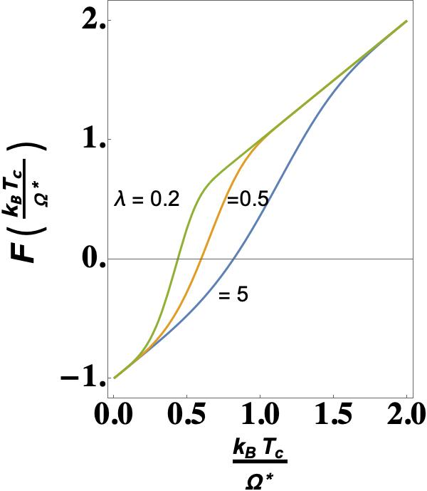
Figure 6: Plot of the function $F[u]=u-\Theta^{\left({u^{4}}/{\lambda}\right)}$ of Eq.(82), vs $u=\frac{k_{B}T_{c}}{\Omega^{*}}$, for various values of the exponent $u^{4}/\lambda$, where $\lambda\propto W\>|g|^{2}{\cal{T}}_{Q}^{2}/U_{c}$ $(=5,0.5,0.2)$ is defined in the text. The plot is for $\Theta=0.1$. The zeros of $F[u]$ provide the critical temperature $T_{c}$.

VII Conclusions

Hopefully, the intriguing high temperature "strange metal" phase of materials undergoing a HTc superconducting transition is at a turning point, since attention was drawn to the "universal" linear dependence on $T$ of the resistivity and to features like the possible violation of the Wiedemann and Franz lawHill et al. (2001); Lavasani et al. (2019). The Wiedemann and Franz universal ratio unambiguously rests on the coexistence of heat and charge transport typical of weakly interacting electronic Fermi Liquids. It is accepted that interactions in these systems are strong and play a nonperturbative role. This gives credit to a Non Fermi Liquid (NFL) perspective for the high temperature normal "bad metal" phase. Consensus in the physics community increases on the use of the doped Mott insulator paradigm as an interpretation ground for the copper oxide HTc materialsCarlson et al. (2002). On the other hand, strong crystal anisotropy and doping tend to privilege the role of copper-oxide planes and the role of collective fluctuations. Even when clean single crystals are availableSreedhar et al. (2020), the doping and the chemistry of the charge reservoir layers separating the CuO2 plane(s) from one another could induce inhomogeneities.

It was really a twist the discovery that the Su-Ye-Kitaev model, in the limit of strong interactions and strong disorder, can be solved exactly in 0+1 dimension displaying a NFL incoherent toy system, with non trivial properties as a zero temperature finite entropy and a chaotic behavior at long times. Moreover, hydrodynamical extensions to higher space dimensions provides the linear dependence of the resistivity which has attracted a flurry of interest from the condensed matter community. By contrast, a conventional Eliashberg approach, typical of FL systems has not been seriously questionedChowdhury and Berg (2020b).

On one side we enquire on the influence of a hopping term between neighbouring SYK clusters organized in a $2-d$ lattice. Hopping is assumed to be marginal in a $1/N$ expansion and strong coupling ${\cal{J}}$ limit, with $\beta{\cal{J}}/N$ kept finite. On the other side we study the perturbative effect that the SYK lattice exerts on a FL with delocalized electrons (in the continuum hydrodynamical limit), displaying a well defined Fermi surface and a large Fermi energy. The aim is to characterize the collective excitations of the SYK system in view of identifying the latter as responsible for the superconducting instability via an unidentified mechanism.

There are various ways to extend the SYK model to a lattice and we use one of themSong et al. (2017); Chowdhury et al. (2018); Gu et al. (2017). All of them rest on a disorder average and we assume that self-averaging allows for a translationally invariant approach with wavevector $k\tilde{a}<<1$, where $\tilde{a}$ is the lattice spacing. We focus on the role of the collective fermionic excitations of a SYK dot $\delta g_{m}$ of Matsubara frequency $\omega_{m}$. Among these, there are also incipient Goldstone Modes, which originate from the spontaneous breaking of the conformal symmetry. However, they acquire mass when the first UV correction $\sim{\cal{O}}\left(\frac{N}{\beta{\cal{J}}}\right)$ is included. They are denoted as pseudo Goldstone modes ($pGm$’s) in the textKitaev ; Maldacena and Stanford (2016). The UV correction forces locality in space and time. The real fermionic propagator $\delta g_{m}$ of the IR limit acquires a complex local phase in the extended SYK action, due to minimal compact $U(1)$ coupling. The energy fluctuations driven by these dressed excitations across the lattice can be monitored by investigating the correlations of a local space-time UV "order parameter" of the incoherent phase, an extension of the bilocal two-point propagator $G_{c}$ of the conformal symmetric limit. In a NFL system they can be interpreted as energy density excitations, better than chemical potential fluctuations. In this work our focus was on the nature of these dressed bosonic fluctuations which we nickname as "Q-excitations" and on the response $D^{\beta}$ of the lattice system to perturbations which excite them. In the recent past, the scaling of U(1) RVB models with a gap to both charge and spin excitations has been studiedYe (1998).

We take advantage of the fact that two time (or temperature) scales come into play, the "fast" intradot fermionic $\delta g_{m}$ modes and the "slow" interdot bosonic energy density fluctuations originating from the Q-excitations. This allows us to characterize the dynamics in a range of energies $\sim T_{0}$, where $T_{0}$ is a threshold temperature for efficient thermalization. In this temperature range the Q-excitations are proved to be diffusive when the dynamics induced by the UV correction is appropriately accounted for. Diffusivity arises from the combination of disorder in the SYK dots and hopping in the superlattice. We find the mode-mode correlations in imaginary time $\propto G_{c}G_{c}{\cal{F}}^{-1}$ where ${\cal{F}}$ is the bilocal 4-point propagator, which diverges in the conformal limit, but is made finite when the UV dominant correction is included. The presence of ${\cal{F}}^{-1}$ in the diffusion parameter is the signature of the presence of the $pGm$ and is the main result of this work. The corresponding retarded response function in real time can be derived from the correlations, by analytic continuation to real frequencies $i\>\omega_{m}\to\omega+i0^{+}$. A similar result was derived directly in real timeSong et al. (2017), but without including the role of the $pGm$ and is reproduced in the appendix C. In the real time approach, the factor ${\cal{F}}^{-1}$ does not appear as part of the diffusive pole. The scaling rinormalizes the thermalization temperature $T_{0}$ and the diffusion constant $\tilde{D}_{Q}$, by introducing a lattice length $\tilde{a}_{\ell}\sim\tilde{a}\>T_{0}/T$ and a diffusion time ${\cal{T}}_{Q}$, such that $\tilde{D}_{Q}{\cal{T}}_{Q}\sim\tilde{a}_{\ell}$. A simple quantum approach to the dynamics of the energy fluctuations in presence of damping $\Gamma$ allows for their explicit determination. $\Gamma\sim T$ is the energy broadening of the Q-fluctuation excitation due to relaxation in the lattice. If we resort to the Einstein relations which connects the diffusion coefficient $\tilde{D}_{Q}$ to the transport coefficientsHartnoll (2015), we derive the temperature dependence of these quantities and obtain Eq.(60) which refers to $\tilde{v}\sim\tilde{a}\Gamma$ as a physical (non universal) diffusion velocity. Eq.(60) has to be contrasted with a bound for incoherent systems that has been conjecturedKovtun et al. (2005).

In the study of the correlations, it emerges clearly (see Fig.4) that our approach to the partition function and to the generating functional is only valid for $T\sim T_{0}$, an energy range which we conclude to be well separated with respect to the one $\sim T_{coh}$, the temperature which marks the prevail of the low energy Fermi Liquid. For $T<T_{0}$, entanglement of the dynamics of the $pGm$’s in the SYK dots with the dynamics of the energy fluctuations across the lattice require more sophisticated methods than the factorization used here, in the calculation of the thermodynamic functionals. Still, some qualitative hint is presented in Subsection V.B.

In Section VI.B we assume that the Q-excitations have a role in the superconductive instability at low temperature. A dispersive self-energy for an electronic quantum liquid perturbed by a SYK dot with a local interaction ${\cal{J}}$ turns the FL into a marginal FLShekhter and Varma (2009), with inverse lifetime of the quasiparticles close to the Fermi surface $\propto\omega$. The quasiparticle lifetime influences the mean field superconductive order parameter $\Delta_{\infty}$ at energies above $\Omega^{*}\sim W^{2}/U_{c}$, where $U_{c}$ is cutoff energy for the pairing interaction. The topic, whether the Q-excitations could really play the role of virtual excitations inducing pairing, provided an appropriate attractive coupling is active Lee (2014); Kopnický and Hlubina (2020); Chowdhury and Berg (2020a), is beyond the present state of the art. It is an old idea that an incipient Goldstone mode of an ordered phase can accomplish this task. This possibility was examined in the past and it was concluded that the fluctuations involved would lead to a depression of $T_{c}$Schrieffer (1995). We think that this pattern may not work here for various reasons. Here, indeed, the vertex corrections vanish to lowest approximation order. However, the fluctuations driving the transition do not arise from an incipient order but are non local in time, in a fully disordered system. What we call "order parameter" here is energy relaxational modes which are effectively non local in space and non number conserving in nature, as phonons would be. We have also omitted the influence of long-range Coulomb interactions, which certainly modifies the spectrum of boson density fluctuationsCarlson et al. (2002).

Of course, if the Q-modes play a role, the temperature scale of the superconducting $T_{c}$ is of electronic origin, $\sim\Omega_{c}^{*}$, defined in Eq.(82). $T_{c}$, as derived using the EliashbergEliashberg and McMillanMcMillan (1968) approaches, is not BCS-like and appears as the zeros of a function $F\left[\frac{k_{B}T_{c}}{\Omega_{c}^{*}}\right]$, which is plotted in Fig.6. It also depends on the "low" energy scale $\sim{{\cal{T}}_{Q}^{coh}}^{-1}$, on the lifetime at higher energies of the Cooper-pairing electron charges and on the diffusion length of the Q-excitations. Indeed, the correlation length of the pairs $\xi$ depends on the effective mean square length $\tilde{a}_{\ell}^{2}\sim D_{Q}{\cal{T}}_{Q}$ which identifies the $2-d$ range of the pairing attractive potential. In our model, its temperature dependence is $\tilde{a}_{\ell}^{2}\sim T_{coh}/T$. This suggests a possible experimental check for the surmise that the superconductive instability is driven by the Q-modes in the CuO2 planes. Two possibilities arise: $a)$ multiple order parameters could provide different intervortex interactions for different magnetic field strengths in lowering the temperature. However this possibility requires a two-component Ginzburg-Landau formalism, even when only one divergent length scale is associated with the transition at $T_{c}$Babaev and Speight (2005); Silaev and Babaev (2012). $b)$ a second superconducting phase transition to $Type\>I$ superconductivity takes place, a rather unlikely possibility. Discussion related to case $a)$ arose in connection with superconductivity in the two band $MgB_{2}$Ernst Helmut Brandt and Das (2011); Kogan and Schmalian (2012); Babaev and Silaev (2012).

Appendices

Appendix A Expansion of the action up to second order

We expand Eq.(7) of the Main Text (MT),

$$\frac{I_{a}}{N}=\sum_{x}\left[-\ln Det(G_{o}^{-1}-\Sigma_{x})+\frac{1}{2}\int d\theta_{1}d\theta_{2}\left(\Sigma_{x}(\theta_{1},\theta_{2})\>G_{x}^{*}(\theta_{1},\theta_{2})-\frac{(\beta{\cal{J}})^{2}}{4}\left|G_{x}(\theta_{1},\theta_{2})\right|^{4}\right)\right.$$

$$\left.+\frac{(\beta t_{0})^{2}}{N}\sum_{x^{\prime}nn}\int d\theta_{1}d\theta_{2}\>G_{x}(\theta_{1},\theta_{2})\>G_{x^{\prime}}^{*}(\theta_{1},\theta_{2})\right]$$ (83)

to second order in $\delta\Sigma_{x},\>\delta G_{x},\>\partial_{\tau}\varphi_{x}$:

$$G_{x}(\theta_{1},\theta_{2})=\left(G_{c}(\theta_{1}-\theta_{2})+\delta G(x,\theta_{1}-\theta_{2},\theta_{+}\right))\>e^{i\>\varphi_{x}(\theta_{+})},$$

$$\Sigma_{x}(\theta_{1},\theta_{2})=\left(\Sigma_{c}(\theta_{1}-\theta_{2})+\delta\Sigma(x,\theta_{1}-\theta_{2},\theta_{+})\right)\>e^{i\varphi_{x}(\theta_{+})}.$$

where $\theta_{+}=(\theta_{1}+\theta_{2})/2$. Gauge invariance is exploited, transforming $\Sigma_{x}(\tau_{1},\tau_{2})$ in such a way that the time derivative $\partial_{\tau}\varphi_{x}(\tau)$ appears in the Det, so that the variation of the Det term reads:

$$\frac{1}{2}\ln\>Det\left[G_{o}^{-1}-\Sigma_{c}\right]-\frac{1}{4}{\bf Tr}\left(\left[G_{o}^{-1}-\Sigma_{c}\right]^{-1}\left|i\>\partial_{\tau}\varphi_{x}+\delta\Sigma\right|\right)^{2}\hskip 199.16928pt$$

$$\to\frac{1}{2}\ln\>det\left[G_{o}^{-1}-\Sigma_{c}\right]-\frac{1}{4}{\bf Tr}\left[2\>\Re e\left\{G_{c}\>i\>\partial_{\tau}\varphi_{x}G_{c}\>\delta\Sigma\right\}-\left(G_{c}\partial_{\tau}\varphi_{x}\right)^{2}+\left(G_{c}\delta\Sigma\right)^{2}\right]$$ (84)

Integrals in time are intended in the second term. Close to the conformal symmetry point (using the saddle point equality $\Sigma_{c}={\cal{J}}^{2}G_{c}^{3}$) the second term in the action of Eq.(83) gives:

$$(\Sigma_{c}+\delta\Sigma)(G_{c}+\delta G)-\frac{{\cal{J}}^{2}}{4}(G_{c}+\delta G)^{4}$$

$$\sim\frac{3{\cal{J}}^{2}}{4}G_{c}^{4}+\delta\Sigma\delta G-\frac{3{\cal{J}}^{2}}{2}G_{c}^{2}\delta G^{2}.$$ (85)

Only second order terms will be retained.

We introduce a dimensionless approach: $\theta=2\pi\tau/\beta$ with the substitutions proposed by Kitaev Kitaev and define $K_{c}(\theta_{1},\theta_{2},\theta_{3},\theta_{4})$:

$$g(\tau_{1},\tau_{2})=R_{c}(\tau_{1},\tau_{2})\>G(\tau_{1},\tau_{2}),$$

$$f(\tau_{1},\tau_{2})=R_{c}^{-1}(\tau_{1},\tau_{2})\>\Sigma(\tau_{1},\tau_{2})$$

$$R_{c}(\theta_{1},\theta_{2})=\beta J\sqrt{(q-1)}\left|\tilde{G}_{c}(\theta_{1},\theta_{2})\right|^{\frac{q-2}{2}},$$

$$K_{c}=R_{c}(\theta_{1},\theta_{2})\tilde{G}_{c}(\theta_{1},\theta_{3})\tilde{G}_{c}(\theta_{4},\theta_{2})R_{c}(\theta_{3},\theta_{4})$$ (86)

For $q=4$, the saddle point bilocal field is:

$$G_{c}(\tau)=b\left[\frac{\pi}{\beta\sin\frac{\pi\>\tau}{\beta}}\right]^{\"{\i}\textquestiondown\textonehalf 1/2}\!\!\!\!sign(\tau),\>\>\>\>b^{2}=\frac{1}{2\>J\pi^{1/2}}.$$ (87)

Excluding for the time being the hopping term, the action $I_{a}$ of Eq.(83), expanded up to second order, reads:

$$\frac{\tilde{I}_{2}}{N}=-\frac{1}{2}\langle\delta f|\delta g\rangle-\frac{1}{4}\left[\langle\delta f|K_{c}|\delta f\rangle+2\>\Re e\left\{\langle\delta f|K_{c}|i\>R_{c}^{-1}\partial_{\tau}\varphi_{x}\rangle\right\}+\langle R_{c}^{-1}\partial_{\tau}\varphi_{x}|K_{c}|R_{c}^{-1}\partial_{\tau}\varphi_{x}\rangle\right]-\frac{1}{4}\langle\delta g|\delta g\rangle$$ (88)

We integrate out $\delta f^{\prime}=\delta f+i\>R_{c}^{-1}\>\partial_{\tau}\varphi_{x}$:

$$\sim e^{-\frac{N}{4}\sum_{x}\left[\langle\delta f^{\prime}|K_{c}|\delta f^{\prime}\rangle+2\langle\delta f^{\prime}|\delta g\rangle-2\langle i\>R_{c}^{-1}\>\partial_{\tau}\varphi_{x}|\delta g\rangle\right]}e^{-\frac{1}{4}\langle\delta g|\delta g\rangle}\sim\prod_{x}\>e^{\frac{N}{2}\langle i\>R_{c}^{-1}\>\partial_{\tau}\varphi_{x}|\delta g\rangle}\>e^{\frac{N}{4}\left[\langle\delta g|K_{c}^{-1}-1|\delta g\rangle\right]}.$$ (89)

The second variation of the hopping term (third term in Eq.(83) ), to lowest order can be expanded as follows:

$$\delta G_{c,x}(\tau_{12},\tau_{+})\delta G_{c,x^{\prime}}^{*}(\tau_{34},\tau_{+}^{\prime})=\left[G_{x}(\tau_{1},\tau_{2})\>G_{x^{\prime}}^{*}(\tau_{3},\tau_{4})-G_{c}(\tau_{1}-\tau_{2})\>G_{c}(\tau_{3}-\tau_{4})\right]$$

$$\approx\frac{1}{2}\>G_{c}(\tau_{12})\>\left(e^{-i{\tilde{a}}\cdot\nabla_{x}\left[\varphi_{x}(\tau_{+})-\varphi_{x}(\tau_{+}^{\prime})\right]}-1\right)\>G_{c}(\tau_{34})+c.c.\hskip 170.71652pt$$

$$\to-\frac{1}{2}\>G_{c}(\tau_{12})\left({\tilde{a}}\cdot\nabla_{x}\left[\varphi_{x}(\tau_{+})-\varphi_{x}(\tau_{+}^{\prime})\right]\right)\!\!^{2}\>G_{c}(\tau_{34}),$$ (90)

where only quadratic terms of the exponential have been included, to account for the additional complex conjugate contribution. We approximate $\left[\varphi_{x}(\tau_{+})-\varphi_{x}(\tau_{+}^{\prime})\right]=\left(\tau_{+}-\tau_{+}^{\prime}\right)\partial_{\tau}\varphi_{x}(\tau_{+})$ and define $R_{c}^{-1}\Lambda_{c}R_{c}^{-1}=\frac{1}{2}({\tilde{a}}\cdot\overset{\leftarrow}{\nabla}_{x})G_{c}(\tau_{12})(\tau_{+}-\tau_{+}^{\prime})^{2}G_{c}(\tau_{34})({\tilde{a}}\cdot\overset{\rightarrow}{\nabla}_{x^{\prime}})$, so that, with relative time integrals traced out,

$$\int\!d\tau\!\!\int\!d\tau^{\prime}\>\partial_{\tau}\varphi_{x}(\tau)R_{c}^{-1}\>\Lambda_{c}(\tau-\tau^{\prime})\>R_{c}^{-1}\partial_{\tau}\varphi_{x}(\tau^{\prime}).$$ (91)

Fourier transform of the time dependences gives $\ \Lambda_{c}\left(\omega_{m},\omega_{m^{\prime}};\Omega_{\ell}\right)$. Fourier transforming the hopping term w.r.to $x$ we obtain the kinetic term added to the action of Eq.(88) so that the full functional integral is:

$$\propto\prod_{p}\int\left(\Pi_{m}\delta g^{*}_{m}\right)\left(\Pi_{m^{\prime}}\delta g_{m^{\prime}}\right)\>e^{\frac{N}{2}\langle i\>R_{c}^{-1}\>\partial_{\tau}\varphi_{x}|\delta g\rangle}\>e^{\frac{N}{4}\left[\langle\delta g|K_{c}^{-1}-1|\delta g\rangle\right]}\>e^{-\frac{N}{2}{t_{0}}^{2}k^{2}\tilde{a}^{2}\left[\langle-i\>R_{c}^{-1}\partial_{\tau}\varphi_{p}|\Lambda_{c}|-i\>R_{c}^{-1}\partial_{\tau}\varphi_{p}\rangle\right]}$$ (92)

where the forks $\langle...\rangle$ denote integration over $(\tau(12)_{+}-\tau(34)_{+})$.

In the conformal limit $i\>\omega_{m}$ can be dropped in $G_{0}^{-1}$in Eq.(83) and the functional integral of Eq.(92) is just a gaussian form, so that, integrating out the $\delta g$’s we have:

$$\sim\prod_{p}e^{-\frac{N}{2}\left\langle-i\>R_{c}^{-1}\>\partial_{\tau}\varphi_{p}\left|\left[K_{c}^{-1}-1\right]^{-1}\right|-i\>R_{c}^{-1}\>\partial_{\tau}\varphi_{p}\right\rangle}\>e^{\frac{N}{4}\>\frac{{t_{0}}^{2}}{N}\>p^{2}\left[\langle-i\>R_{c}^{-1}\partial_{\tau}\varphi_{p}|\Lambda_{c}|-i\>R_{c}^{-1}\partial_{\tau}\varphi_{p}\rangle\right]}$$

$$\sim\prod_{p}e^{-\frac{N}{2}\left\langle-i\>R_{c}^{-1}\>\partial_{\tau}\varphi_{p}\left|\left(1-\frac{{t_{0}}^{2}}{N}p^{2}\Lambda_{c}[1-K_{c}]\right)K_{c}\left[1-K_{c}\right]^{-1}\right|-i\>R_{c}^{-1}\>\partial_{\tau}\varphi_{p}\right\rangle}\>$$

$$\sim\prod_{p}e^{-\frac{N}{2}\left\langle-i\>\partial_{\tau}\varphi_{p}\left|\left(1-\>\ \frac{t_{0}^{2}}{N}{p^{2}}R_{c}^{-1}\Lambda_{c}R_{c}^{-1}{\cal{F}}^{-1}\right){\cal{F}}\right|-i\>\partial_{\tau}\varphi_{p}\right\rangle}.$$ (93)

Here we have defined ${\cal{F}}=R_{c}^{-1}\>K_{c}[K_{c}-1]^{-1}\>R_{c}^{-1}$, and in the Kernel of Eq.(93) we write:

$$R_{c}^{-1}K_{c}[1-K_{c}]^{-1}R_{c}^{-1}-\frac{t_{0}^{2}}{N}R_{c}^{-1}\Lambda_{c}[1-K_{c}]K_{c}^{-1}K_{c}[1-K_{c}]^{-1}R_{c}^{-1}=\left(1-\>\ \frac{t_{0}^{2}}{N}{p^{2}}R_{c}^{-1}\Lambda_{c}R_{c}^{-1}{\cal{F}}^{-1}\right){\cal{F}}.\hskip 28.45274pt$$ (94)

The numerical evaluation of this kernel is discussed in B.

Appendix B Numerical evaluation of the Kernel of Eq.(94)

The correlator ${\cal{F}}=R_{c}^{-1}\>K_{c}[K_{c}-1]^{-1}\>R_{c}^{-1}$ has been defined after Eq.(93). It diverges in the conformal limit because $[K_{c}-1]$ has zero eigenvalues due to the spontaneous symmetry breaking. We will keep just the series of these eigenvalues (usually denoted by $h=2$), which make the largest contribution to the correlator functions. The spectral representation in imaginary time of the regularized form of the kernel, obtained by shifting the zero eigenvalues, $k(h=2,n)\approx 1-\frac{\alpha_{K}}{\beta{\cal{J}}}|n|+...$($\alpha_{K}\approx 3$), thus including the UV correction at ${\cal{O}}\left(N/\beta{\cal{J}}\right)$ is Maldacena and Stanford (2016)

$$K_{c}[1-K_{c}]^{-1}=\frac{1}{2}R_{c}(\tau_{12})\>{\cal{F}}\left(\tau_{12},\tau_{34}\right)\>R_{c}(\tau_{34})$$

$$=\sum_{h,n}\Psi_{h,n}(\tau_{12})\frac{k(h,n)}{1-k(h,n)}\Psi_{h,n}^{*}(\tau_{34}).$$

The basis functions for $h=2$ are

$$\Psi_{2\>n}(x,y)=\gamma_{n}\frac{e^{-i\>ny}}{2\sin\frac{x}{2}}\>f_{n}(x),$$

$$f_{n}(x)=\frac{\sin\frac{nx}{2}}{\tan\frac{x}{2}}-n\>\cos\frac{nx}{2},\>\>\>\gamma_{n}^{2}=\frac{3}{\pi^{2}|n|(n^{2}-1)},$$ (95)

with $x_{12}=\tau_{1}-\tau_{2},\>\>\>\>y_{12}=\frac{\tau_{1}+\tau_{2}}{2}$. We Fourier transform the variables $\tau_{12}$ and $\tau_{34}$. In full generality:

$${\cal{O}}_{m,m^{\prime}}=\sum_{n\geq 2}e^{i\>n(y_{12}-y_{34})}\Phi_{n}(\omega_{m})\left\langle 2,n\left|{\cal{O}}\right|2,n\right\rangle\Phi_{n}^{*}(\omega_{m^{\prime}}),$$

where $\omega_{m},\omega_{m^{\prime}}$ are the fermionic Matsubara frequencies. We ridefine variables in such a way that $\omega_{m}\to m$ with $m$ integer. The basis functions are:

$$\Phi_{n}(m)=\int_{0}^{2\pi}\frac{d\tau}{2\pi}\>\frac{1}{\sin\frac{\tau}{2}}\>f_{n}(\tau)\>e^{i\>m\>\tau}.$$ (96)

It can be shown that the Fourier transforms $\Phi_{n}(m)$ have a factor $-\frac{1}{2}\left(1+e^{2\>i\>m\pi}\right)$ or $-\frac{1}{2}\left(1-e^{2\>i\>m\pi}\right)$, depending on $n$ being even or odd, respectively. It follows that odd $m$ imply even $n$ as expected because the $\tau_{+}$ time dependence has to be with $n$ even, i.e. bosonic-like. $\Phi_{n}(m)$ have a maximum at increasing values of $m$ when $n$ increases and eventually go to zero.

The largest contribution ${\cal{O}}(\beta{\cal{J}}/N)$ of $\left[1-K_{c}\right]^{-1}$ appearing in Eq.(93), gives $R_{c}^{-1}K_{c}\left[1-K_{c}\right]^{-1}R_{c}^{-1}\sim{\cal{O}}(1)$ and, as $G_{c}G_{c}\sim 1/\beta{\cal{J}}$, to have the same order of the kinetic term $t_{0}\sim{\cal{O}}([\beta{\cal{J}}/N]^{1/2})$.

In the definition of the matrix function $R_{c}^{-1}\Lambda_{c}R_{c}^{-1}$ from Eq.(11), the matrix $\widehat{G_{c}G_{c}}\hat{{\cal{F}}}^{-1}$ appears, which is the inverse of $\frac{{\cal{F}}}{G_{c}G_{c}}$.

The dominant expression for $\frac{{\cal{F}}}{G_{c}G_{c}}(\tau_{1}...\tau_{4})$ in imaginary times, on the subspace orthogonal to the $pGm$ fluctuations is Maldacena and Stanford (2016):

$$\frac{{\cal{F}}}{G_{c}G_{c}}(\tau_{1}...\tau_{4})=\frac{6\alpha_{0}}{\pi^{2}\alpha_{K}}\beta{\cal{J}}\!\!\sum_{n\geq 2}\!\frac{e^{i\>n(y_{12}-y_{34})}}{n^{2}(n^{2}-1)}\>f_{n}(\tau_{12})\>f_{n}(\tau_{34}).$$ (97)

Its Fourier transform requires the transformed basis functions:

$$\phi_{n}(m)=\int_{0}^{2\pi}\frac{d\tau}{2\pi}\>f_{n}(\tau)\>e^{i\>m\>\tau}.$$

All of them have a factor $\sin{m\pi}$ which vanishes for $m$ odd integer. However, this zero can be compensated by a zero in the denominator. Consider the case $n=2$ for example:

$$\phi(n=2,m)=\frac{\sin{m\pi}}{\pi\>m(m-1)(m+1)}\>e^{im\pi},$$

We give a finite expression to this vector element using the limit:

$$\lim_{x=\pm 1}\frac{\sin x\pi}{(x-1)(x+1)}=\frac{1}{2}(\mp\pi),$$ (98)

However, all $m>1$ give zero for $n=2$, because there is no other factor of the kind $(m-3),(m-5),...$(only odd $m$ are considered) in the denominator. We get $\phi_{n}(m)=\>sign(m)\times$:

$$n=2\>\>\>\quad\quad\mathbf{\Rightarrow}\quad \left\{\begin{array}[]{cc}m=1&\frac{1}{2\>m^{2}}\>e^{im\pi},\\ m=3,5,7,...&0\end{array}\right.$$ (101)

$$n=4\>\>\>\quad\quad\mathbf{\Rightarrow}\quad \left\{\begin{array}[]{cc}m=1&-2\>\frac{(5m^{2}-2)}{(m-2)(m+2)}\>\frac{1}{2\>m^{2}}\>e^{im\pi}\\ m=3,5,7,...&0\end{array}\right.$$ (104)

$$n=6\>\>\>\quad\quad\mathbf{\Rightarrow}\quad \left\{\begin{array}[]{cc}m=1&-\>\frac{(36-119m^{2}+35m^{4})}{(m-3)(m-2)(m+2)(m+3)}\>\frac{1}{2\>m^{2}}\>e^{im\pi}\\ m=3&-\>\frac{(36-119m^{2}+35m^{4})}{(m-2)(m-1)(m+1)(m+2)}\>\frac{1}{2\>m^{2}}\>e^{im\pi}\\ m=5,7,9,...&0\end{array}\right.$$ (108)

$$n=8\>\>\>\quad\quad\mathbf{\Rightarrow}\quad \left\{\begin{array}[]{cc}m=1&-\>\frac{2\>(-288+1068m^{2}-462m^{4}+42m^{6})}{(m-4)(m-3)(m-2)(m+2)(m+3)(m+4)}\>\frac{1}{2\>m^{2}}\>e^{im\pi}\\ m=3&-\>\frac{2\>(-288+1068m^{2}-462m^{4}+42m^{6})}{(m-4)(m-2)(m-1)(m+1)(m+2)(m+4)}\>\frac{1}{2\>m^{2}}\>e^{im\pi}\\ m=5,7,9,...&0\end{array}\right.$$ (112)

$$n=10\>\>\>\quad\quad\mathbf{\Rightarrow}\quad \left\{\begin{array}[]{cc}m=1&-\>\frac{3\>(-4800+18964m^{2}-9735m^{4}+1386m^{6}+55m^{8})}{(m-5)(m-4)(m-3)(m-2)(m+2)(m+3)(m+4)(m+5)}\>\frac{1}{2\>m^{2}}\>e^{im\pi}\\ m=3&-\>\frac{3\>(-4800+18964m^{2}-9735m^{4}+1386m^{6}+55m^{8})}{(m-5)(m-4)(m-2)(m-1)(m+1)(m+2)(m+4)(m+5)}\>\frac{1}{2\>m^{2}}\>e^{im\pi}\\ m=5&-\>\frac{3\>(-4800+18964m^{2}-9735m^{4}+1386m^{6}+55m^{8})}{(m-4)(m-3)(m-2)(m-1)(m+1)(m+2)(m+3)(m+4)}\>\frac{1}{2\>m^{2}}\>e^{im\pi}\\ m=7,9,11,...&0\end{array}\right.$$ (117)

$$n=12\>\>\>\quad\quad\mathbf{\Rightarrow}\quad \left\{\begin{array}[]{cc}m=1&=-\>\frac{2(-259200+1066104m^{2}-603746m^{4}+105963m^{6}-6864m^{8}+143m^{10})}{(m-5)(m-4)(m-3)(m-2)(m+2)(m+3)(m+4)(m+5)}\>\frac{1}{2\>m^{2}}\>e^{im\pi}\\ m=3&-\>\frac{2(-259200+1066104m^{2}-603746m^{4}+105963m^{6}-6864m^{8}+143m^{10})}{(m-5)(m-4)(m-2)(m-1)(m+1)(m+2)(m+4)(m+5)}\>\frac{1}{2\>m^{2}}\>e^{im\pi}\\ m=5&-\>\frac{2(-259200+1066104m^{2}-603746m^{4}+105963m^{6}-6864m^{8}+143m^{10})}{(m-4)(m-3)(m-2)(m-1)(m+1)(m+2)(m+3)(m+4)}\>\frac{1}{2\>m^{2}}\>e^{im\pi}\\ m=7,9,11,...&0\end{array}\right.$$ (122)

Also the polynomials in the numerator could have been factorized but the roots are non-integer. We normalize each $n-$vector of the basis but we do not orthogonalize these basis vectors. We define matrices $W^{n}_{m,m^{\prime}}$, by multiplying $column\times row$ each $n-$vector.To the elements with $m,m^{\prime}=1$, all vectors $n=2,4,6,8,10,12$ contribute. To the elements with $m,m^{\prime}=3$, vectors with $n=4,6,8,10,12$ contribute. To the elements with $m,m^{\prime}=5$ only vector with $n=10,12$ contributes. The final result for $n\leq 12$ is a $3\times 3$matrix. Each $3\times 3$ matrix $\hat{W}^{n}$ has eigenvalues $1,0,0$. Computations leading to Fig.2,3,4 of the MT have been performed with $3\times 3$ matrices up to $n=12$. The starting point is Eq.(20) of the text:

$$\left.\frac{{\cal{F}}}{G_{c}G_{c}}\left(y_{12}-y_{34}\right)\right|_{m,m^{\prime}}=\frac{6\alpha_{0}}{\pi^{2}\alpha_{K}}\beta{\cal{J}}\sum_{n\geq 2,even}^{10}\frac{\cos{n(y_{12}-y_{34})}}{n^{2}(n^{2}-1)}\>W^{n}_{m,m^{\prime}}.$$

where $y$ are center-of-mass times: $y=y_{12}-y_{34}$.

In Fig.4 of the MT we plot an interpolated smoothed curve of the (approximate) lowest $\overline{M}$ value which fulfills unitarity of the partition function of Eq.(46) of MT vs. $T_{0}/T$, for $k\tilde{a}=1$. Precision is up to $>10^{-5}$. The trend is only meaningful for $T_{0}/T\sim 1$, because larger values require $n>12$ in the spectral representation of Eq.(97) and matrices $m\times m$ of rank $\tilde{r}>3$, i.e. higher than the ones used here.

Appendix C Real time approach to the correlation functions

The response function in real time is derived from extension of the imaginary time along the Keldysh contour. The present approachSong et al. (2017) is only semiclassical. In setting up the functional we disregard the $q-q$ term and neglect variation with respect to the saddle point solutions for the $G$ and $\Sigma$ of the SYK dots. This means that, in going back to the action in Eq.(88), terms with $\delta g$ and $\delta f$ are disregarded, so that only an extra term is added here, taken from the imaginary time action, that is $-\frac{N}{4}\langle R_{c}^{-1}\partial_{\tau}\varphi_{x}|K_{c}|R_{c}^{-1}\partial_{\tau}\varphi_{x}\rangle=-\frac{N}{4}\langle\partial_{\tau}\varphi_{x}|G_{c}G_{c}|\partial_{\tau}\varphi_{x}\rangle$, which we denote as the kinetic energy term.

As for the non local phase fluctuations, Fourier transforming with respect to time the non local fluctuation part of the action (i.e. the "hopping" term of Eq.(91)) is of a similar form:

$${\scriptstyle\int dp\>\tilde{D}\>p^{2}\>\sum_{ss^{\prime}}\int d\omega\>\varphi_{s}(\omega)\>ss^{\prime}\>G_{ss^{\prime\prime}}(\omega)\>G_{s^{\prime\prime}s^{\prime}}(-\omega)\>\varphi_{s^{\prime}}(-\omega)}.$$ (124)

With respect to the Fourier transform of the kinetic energy term, the present one has a factor $\omega^{2}$ lacking, so that we merge the two together, by defining a function

$$\left[\frac{\tilde{D}\>p^{2}\>h(\omega)}{\omega^{2}}-1\right]\>G_{c}G_{c}\equiv\zeta\>G_{c}G_{c}.$$ (125)

which defines the function $\zeta(\omega)$. $h(\omega)$ excludes the $\omega=0$ term. Its retarded form is defined as

$$\tilde{D}\>\>h_{R}(\omega)\>G^{R}_{\omega}G^{K}_{-\omega}=\tilde{D}\>\int_{-\infty}^{\infty}dt\>G^{R}(t)G^{K}(-t)\>\left[e^{i\>\omega t}-1\right]$$

$$\sim i\>\tilde{D}\>\>\omega\>\int_{-\infty}^{\infty}dt\>G^{R}(t)G^{K}(-t)\approx i\>\tilde{D}\>\>\omega\>G^{R}_{0}G^{K}_{0}.$$

When writing $h(\omega)$, we will not specify the label $R/A$ for the retarded or advanced form, in the following, as long as no ambiguity arises. Transforming from the branches $s,s^{\prime}=+,-$ to the combined $\alpha,\beta\equiv cl,q$Kamenev and Levchenko (2009); Belzig et al. (1999), we get:

$$\varphi^{cl/q}(t_{j})=\frac{1}{\sqrt{2}}\left(\varphi_{+}(t_{j})\pm\varphi_{-}(t_{j})\right),$$

$$\frac{1}{2}\left(\begin{array}[]{cc}1&1\\ 1&-1\end{array}\right)\>\left(\begin{array}[]{cc}G_{++}&G_{+-}\\ G_{-+}&G_{--}\end{array}\right)\>\left(\begin{array}[]{cc}1&1\\ 1&-1\end{array}\right)=\left(\begin{array}[]{cc}0&G^{A}\\ G^{R}&G^{K}\end{array}\right).$$ (134)

The $cl-cl$ component is zero in the matrices on the right. It reflects the fact that for a pure classical field configuration ($\varphi^{q}=0$), the action is zero. Indeed, in this case $\varphi_{+}=\varphi_{-}$ and the action on the forward part of the contour is canceled by that on the backward part (safe for the boundary terms, that may be omitted in the continuum limit), because the circuit is closedKamenev and Levchenko (2009).

The integrand of Eq.(124) becomes Song et al. (2017):

$$\begin{array}[]{cc}\left(\>\varphi^{c}_{\omega}\right.&\left.\varphi^{q}_{\omega}\right)\\ &\end{array}\>\left(\begin{array}[]{cc}G^{A}_{\omega}\>G^{R}_{-\omega}&G^{A}_{\omega}G^{K}_{-\omega}\\ G^{K}_{\omega}G^{R}_{-\omega}&G^{R}_{\omega}G^{A}_{-\omega}+G^{K}_{\omega}G^{K}_{-\omega}\end{array}\right)\left(\begin{array}[]{c}\varphi^{c}_{-\omega}\\ \varphi^{q}_{-\omega}\end{array}\right)$$ (141)

The resulting matrix can be rewritten as matrix of the self-energies ${\Sigma}_{D}$ due to the $\tilde{D}\>$ coupling, which shows the same causality structure:

$$\left(\begin{array}[]{cc}G^{A}_{\omega}\>G^{R}_{-\omega}&G^{A}_{\omega}G^{K}_{-\omega}\\ G^{K}_{\omega}G^{R}_{-\omega}&G^{R}_{\omega}G^{A}_{-\omega}+G^{K}_{\omega}G^{K}_{-\omega}\end{array}\right)=\left(\begin{array}[]{cc}G^{A}_{\omega}\>G^{R}_{-\omega}&{\Sigma}_{{D}}^{A}\\ {\Sigma}_{{D}}^{R}&{\Sigma}_{{D}}^{K}\end{array}\right).$$ (146)

We neglect the ${qq}$ term and write the functional:

$$\int{\cal{D}}\varphi^{c}_{\omega}{\cal{D}}\varphi^{q}_{\omega}\>e^{\begin{array}[]{cc}-\frac{i}{2}\int d\omega\>\left(\omega\>\varphi^{c}_{\omega}\right.&\left.\omega\>\varphi^{q}_{\omega}\right)\\ &\end{array}\>\left(\begin{array}[]{cc}G^{A}_{\omega}\>G^{R}_{-\omega}&\zeta^{A}\>G^{A}_{\omega}G^{K}_{-\omega}\\ \zeta^{R}\>G^{K}_{\omega}G^{R}_{-\omega}&0\end{array}\right)\left(\begin{array}[]{c}\omega\varphi^{c}_{-\omega}\\ \omega\varphi^{q}_{-\omega}\end{array}\right)},$$ (153)

where we have also added the kinetic energy term of the semiclassical approach.

The field ${\dot{\cal{N}}}(x,t)$ is the source of $\partial_{t}\varphi(x,t)$. We want the response written along the Keldysh contour:

$$D_{{\dot{\cal{N}}}{\dot{\cal{N}}}}(x,t)=i\>\theta(t)\langle\left[{\dot{\cal{N}}}(x,t),{\dot{\cal{N}}}(0,0)\right]\rangle$$

$$=\frac{i}{2}\langle\left\{{\dot{\cal{N}}}^{c}(x,t){\dot{\cal{N}}}^{q}(0,0)+{\dot{\cal{N}}}^{q}(x,t){\dot{\cal{N}}}^{c}(0,0)\right\}\rangle.$$ (154)

To get the generating functional of the $\varphi-\varphi$ fluctuations we invert the kernel of Eq.(153), obtaining the matrix:

$$\left(\begin{array}[]{cc}0&(\zeta^{R}G^{K}_{\omega}G^{R}_{-\omega})^{-1}\\ (\zeta^{A}G^{A}_{\omega}G^{K}_{-\omega})^{-1}&-(G^{K}_{\omega}G^{K}_{-\omega})^{-1}\end{array}\right)$$ (157)

The $[G^{-1}]^{K}$ component for the free field is only a regularization factor, originating from the (time) boundary terms. It is, in general, non-local in $x$ and $x^{\prime}$, however, being a pure boundary term, it is frequently omittedKamenev and Levchenko (2009). In our case this should apply because $[G^{-1}]^{K}(t,t^{\prime})=[G^{-1}]^{R}\circ F-F\circ[G^{-1}]^{A}=[G^{R}]^{-1}\circ F-F\circ[G^{A}]^{-1}=[G^{K}]^{-1}$ . Integrating out the $\varphi$ fields and ignoring again the $q-q$ term, we get:

$$\propto\exp\left\{\begin{array}[]{cc}-\frac{1}{2}\int d\omega\>\left({\dot{\cal{N}}}^{c}(\omega)\right.&\left.{\dot{\cal{N}}}^{q}(\omega)\right)\\ &\end{array}\left(\begin{array}[]{cc}0&(\zeta^{R}G^{K}_{\omega}G^{R}_{-\omega})^{-1}\\ (\zeta^{A}G^{A}_{\omega}G^{K}_{-\omega})^{-1}&0\end{array}\right)\>\left(\begin{array}[]{c}{\dot{\cal{N}}}^{c}(-\omega)\\ {\dot{\cal{N}}}^{q}(-\omega)\end{array}\right)\right\}.$$ (164)

Functional derivation with respect to the sources provides the cross contributions (we keep just the lowest order in $\omega$). Using the definition of Eq.(125):

$$N\omega^{2}\langle\varphi^{cl}(\omega)\>\varphi^{q}(-\omega)\rangle\approx\>(G^{K}_{0}G^{R}_{0})^{-1}\>\frac{\omega^{2}}{i\>\tilde{D}\>p^{2}\omega-\omega^{2}}$$

$$N\omega^{2}\langle\varphi^{q}(\omega)\>\varphi^{cl}(-\omega)\rangle\approx\left(G^{A}_{0}G^{K}_{0}\right)^{-1}\>\frac{\omega^{2}}{-i\>\tilde{D}\>p^{2}\omega-\omega^{2}}.$$

Now, the retarded energy flux density response of Eq.(154) can be estimated, considering that $\delta\dot{\varphi}^{c,q}$ and ${\dot{\cal{N}}}^{c/q}$ are conjugate variables ${\dot{\cal{N}}}^{c/q}(t)=\frac{\delta S_{\varphi}}{\delta\dot{\varphi}^{c,q}},$ so that, keeping just the $\omega^{2}-$term in Eq.(153),

$${\dot{\cal{N}}}^{cl}(\omega)=-N\>G^{A}_{0}G^{K}_{0}\omega\varphi_{q}(-\omega),$$

$${\dot{\cal{N}}}^{q}(\omega)=-N\>G^{K}_{0}G^{R}_{0}\omega\varphi_{cl}(-\omega)$$

we get

$$\langle{\dot{\cal{N}}}^{cl}(\omega)\>{\dot{\cal{N}}}^{q}(-\omega)\rangle=-N^{2}\>G^{A}_{0}G^{K}_{0}\>G^{K}_{0}\>G^{R}_{0}\>\omega^{2}\times\langle\varphi^{q}(-\omega)\varphi^{cl}(\omega)\rangle\>$$

$$=-N^{2}\>\frac{\omega^{2}}{i\>t_{0}^{2}p^{2}\omega-\omega^{2}}\>G^{A}_{0}G^{K}_{0},\>$$

$$\langle{\dot{\cal{N}}}^{q}(\omega)\>{\dot{\cal{N}}}^{cl}(-\omega)\rangle=-N^{2}\>G^{K}_{0}G^{R}_{0}\>\omega^{2}\times\>\langle\varphi^{cl}(-\omega)\varphi^{q}(\omega)\rangle\>G^{A}_{0}G^{K}_{0}\>$$

$$=-N^{2}\>\frac{\omega^{2}}{-i\>t_{0}^{2}p^{2}\omega-\omega^{2}}\>G^{K}_{0}G^{R}_{0}.$$

The symmetrized correlation is:

$$\frac{1}{2}\>\left(\langle{\dot{\cal{N}}}^{cl}(\omega)\>{\dot{\cal{N}}}^{q}(-\omega)\rangle+\langle{\dot{\cal{N}}}^{q}(\omega)\>{\dot{\cal{N}}}^{cl}(-\omega)\rangle\right)=N^{2}\>\Re e\left\{\frac{\omega^{2}}{i\>t_{0}^{2}p^{2}\omega+\omega^{2}}\>G^{K}_{0}G^{R}_{0}\right\}$$

$$\approx N^{2}\>\frac{t_{0}^{2}p^{2}\omega\>}{(t_{0}^{2}p^{2})^{2}+\omega^{2}}\>\Im m[G^{K}_{0}G^{R}_{0}].$$ (165)

This result can be rewritten as

$$sign(\omega)\>\Im m\left\{\frac{\omega}{i\>t_{0}^{2}p^{2}-\omega}\>\Im m[G^{K}_{0}G^{R}_{0}]\right\}.$$

Subtracting the $p=0$ term, we recognize $\Im m\{D^{R}(p,\omega)\}$, the imaginary part of the density response functionWen (2010)

$$\Im m\left\{D^{R}_{{\dot{\cal{N}}}{\dot{\cal{N}}}}(p,\omega)\right\}=-sign(\omega)\>\Im m\left\{\left(\frac{D\>p^{2}}{i\>\omega-D\>p^{2}}\right)\>\Im m[G^{K}_{0}G^{R}_{0}]\right\}.$$ (166)

This result should be compared with Eq.(51) of the MT. Apart for the matrix structure of the function in Eq.(47) of the MT, the important point is that ${\cal{F}}^{-1}$ is absent here in the definition of the diffusion parameter.

We add here the important consequence on the electrical conductivity. In the conformal limit, the electrical conductivity is Song et al. (2017):

$$Re\{\sigma\}=-\lim_{\omega\to 0}\>\frac{1}{\omega}\Im m\left\{D^{R\beta}(\omega)\right\}\propto-\frac{\beta}{2\pi^{2}}\>\frac{t_{0}^{2}}{N}\int d\omega\>{\rm sech}^{2}\frac{\beta\omega}{2}\>\left(\Im m\left\{G^{R\beta}(\omega)\right\}\right)^{2}$$

$$=-\frac{1}{2\pi^{3/2}}\>\frac{t_{0}^{2}}{N\epsilon}\>\int dx\>{\rm sech}^{2}(\pi x)\>\left[\Re e\left\{\frac{\Gamma\left(\frac{1}{4}-i\>x\right)}{\Gamma\left(\frac{3}{4}-i\>x\right)}\right\}\right]^{2}\propto\left(\frac{\beta{\cal{J}}}{\pi\alpha_{S}N}\"{\i}\textquestiondown\textonehalf\right).\hskip 156.49014pt$$ (167)

Resistivity is $\propto T$ in this approach.

Appendix D Quantization of gapless diffusive excitation mode

$J_{\cal{Q}}=-\kappa\nabla T$ is a classical diffusion equation of a non conserving system. We now construct a Hamiltonian of the excitation modes which is conserving but we ask that, introducing a relaxation time $\tau_{0}=\hbar/\Gamma$ for these modes, the equation of motion reproduces $J_{\cal{Q}}=-\kappa\nabla T$. We will quantize this Hamiltonian and derive the response function from the fluctuations of these modes. The canonical conjugate variables and the corresponding Lagrangian (in 2-d) are:

$$\dot{\theta}=\left(\frac{\kappa C}{\hbar T}\right)^{1/2}\!\!\frac{J_{\cal{Q}}\tau_{0}}{k_{B}},\>\>\nabla\theta=\left(\frac{\hbar}{\kappa C\>T}\right)^{1/2}\!\!\frac{\kappa}{T}\nabla T$$ (168)

Here $C$ is the thermal capacitance, $\kappa$ is the thermal conductance and $J_{Q}$ is is the thermal energy current . The corresponding Lagrangian is

$${\cal{L}}=\frac{1}{2}\int d^{2}x\>\left[\frac{k_{B}}{T}\>\left(\frac{J_{\cal{Q}}\tau_{0}}{k_{B}}\right)^{2}+\frac{\hbar}{\kappa C}\>\left(\frac{\kappa}{T}\nabla T\right)^{2}\right]$$

$$\equiv\frac{1}{2}\int d^{2}x\>\left[A\>\dot{\theta}^{2}+B\>(\nabla\theta)^{2}\right]$$ (169)

with $A=\frac{\hbar k_{B}}{\kappa C}$ and $B=T$. These choices provide terms in the square brackets which have dimension ${\cal{E}}/\ell^{2}$ (${\cal{E}}\equiv\>energy$).

With the approximation $\tau_{0}\dot{J}_{\cal{Q}}\approx{J}_{\cal{Q}}$, the equation of motion,

$$\frac{d}{dt}\left(\frac{\partial L}{\partial\dot{\theta}}\right)-\frac{\partial L}{\partial\nabla\theta}=A\ddot{\theta}+B\nabla\theta=0,$$ (170)

boils down to the diffusion equation:

$$\frac{\hbar}{\kappa C}\>J_{\cal{Q}}=-\frac{\hbar}{\kappa C}\>\kappa\nabla T.$$

Although $\hbar$ is already in the Lagrangian, we proceed with quantization of the theory Wen (2010). Fourier transforming, the canonical momentum for $\theta_{k}$ is

$$\pi_{k}=\frac{\partial{\cal{L}}}{\partial\dot{\theta}_{k}}=A\dot{\theta}_{-k},\>\>\>\left[\theta_{k},\pi_{k^{\prime}}\right]=i\>\delta_{kk^{\prime}}.$$ (171)

The Hamiltonian

$${\cal{H}}=\frac{1}{2}\sum_{k}\left[\frac{1}{A}\pi_{-k}\pi_{k}+Bk^{2}\>\theta_{-k}\theta_{k}\right].$$

is second quantized according to $\hat{a}_{k}=u_{k}\theta_{k}+i\>v_{k}\>\pi_{-k}$, with

$$u_{k}=\frac{1}{\sqrt{2}}\left(AB\right)^{1/4},\>\>v_{k}=\frac{1}{\sqrt{2}}\left(AB\right)^{-1/4},$$

$$\epsilon_{k}=\sqrt{\frac{B\>k^{2}}{A}}=\left[\frac{\kappa}{k_{B}}\frac{CT}{\hbar}\right]^{1/2}|k|\equiv v\>|k|,$$ (172)

$$\pi_{k}=-i\>T^{1/2}\frac{1}{(2\epsilon_{k})^{1/2}}|k|\>\left(\hat{a}_{-k}-{\hat{a}}^{\dagger}_{k}\right),$$

$$\theta_{k}=T^{-1/2}\frac{(2\epsilon_{k})^{1/2}}{|k|}\>\left(\hat{a}_{k}+{\hat{a}}^{\dagger}_{-k}\right)$$ (173)

$${\cal{H}}=\sum_{k}\epsilon_{k}\>{\hat{a}}^{\dagger}_{k}\hat{a}_{k}+cnst$$ (174)

In Eq.(172) we have defined the velocity $v$ of these modes. The approach is similar to the one for phonons. $\pi(x)$ plays the role of the space displacement $d(x,t)$, while $\nabla\theta$ plays the role of the phonon impulse $\Pi(x,t)$. The thermal conductance used in the text is given by

$$\"{\i}\textquestiondown\textonehalf\Re e\{\kappa(\omega)\}=-\frac{1}{\omega}\Im m\!\!\left\{\frac{1}{2}\left\langle\left\{J^{{\cal{Q}}}_{-k}(-\omega),J^{{\cal{Q}}}_{k}(\omega)\right\}\right\rangle\right\}_{(\omega,k=0)}\!\!\!\!\!\!\!\!\!\!\!\!,\>\>$$ (175)

where

$$\frac{1}{2}\left\langle\left\{J^{{\cal{Q}}}_{-k},J^{{\cal{Q}}}_{k}\right\}\right\rangle_{\omega}=\frac{1}{\tau_{0}^{2}}\frac{\kappa CT}{2\hbar}\left\langle\left\{\pi_{-k},\pi_{k}\right\}\right\rangle_{\omega}.$$ (176)

The symmetrized correlation on the right hand side, $D^{\beta}(\omega)=\left\langle\left\{\pi_{-k},\pi_{k}\right\}\right\rangle_{\omega,k=0}$, apart of the prefactor $T$, can be evaluated at zero temperature in a standard way Wen (2010). Eq.(175) gives:

$$\Re e\{\kappa(\omega)\}=\pi^{2}\>k_{B}\frac{\omega\tau_{0}}{v^{2}\tau_{0}^{2}}.$$ (177)

If $\Re e\{\kappa(\omega)\}\sim\kappa\>\tau_{0}$ we get, from Eq.(172),

$$v^{2}\tau_{0}^{2}=\frac{\kappa\tau_{0}}{k_{B}}\>\frac{CT}{\hbar/\tau_{0}}\quad\quad\mathbf{\Rightarrow}\quad\kappa=\frac{\pi k_{B}}{\tau_{0}}\left(\frac{\hbar\omega}{CT}\"{\i}\textquestiondown\textonehalf\right)^{1/2}.$$ (178)

However, introducing the damping of the mode in $D^{\beta}$, by adding an energy broadening $\Gamma$, we get

$$D^{\beta}(\omega)=\frac{\pi T}{v^{4}\Gamma}\int_{0}^{+\infty}\frac{2\>e^{-\epsilon 0^{+}}\>\epsilon}{\epsilon^{2}-\left(\omega+i\>\Gamma\right)^{2}}\>\epsilon^{2}d\epsilon$$ (179)

and

$$\Im m\left\{D^{\beta}(\omega)\right\}=-\frac{2\pi T\>\omega^{2}}{v^{4}\Gamma}\>\left\{\left(1-\frac{\Gamma^{2}}{\omega^{2}}\right)\arctan\frac{\Gamma}{\omega}\"{\i}\textquestiondown\textonehalf+\frac{\Gamma}{\omega}\>\ln\left(1+\frac{\Gamma^{2}}{\omega^{2}}\right)\right\},$$

which, in the limit $\Gamma/\omega<<1$ gives:

$$\Im m\left\{D^{\beta}(\omega)\right\}=-\frac{2\pi T}{v^{4}}\>\omega.$$ (180)

Posing again $\Re e\{\kappa(\omega)\}\sim\kappa\>\tau_{0}$, in place of Eq.(178) we have:

$$v^{2}\tau_{0}^{2}=\frac{\kappa\tau_{0}}{k_{B}}\>\frac{CT}{\hbar/\tau_{0}}\quad\quad\mathbf{\Rightarrow}\quad\kappa=k_{B}\Gamma\left(\frac{h\>\Gamma}{CT}\"{\i}\textquestiondown\textonehalf\right)^{1/2}.$$ (181)

Using the $\kappa=C\>v_{F}\ell=C\>v_{F}^{2}\tau_{0}$, the gapless bosonic excitations of energy $\hbar v\>k$ generate a specific heat at fixed $2-d$ volume:

$$\frac{C_{{\cal{V}}}}{\tilde{a}^{2}}=\frac{d}{dT}\frac{1}{2\pi}\left(\frac{k_{B}T}{\hbar v}\right)^{3}\hbar v\int_{0}^{+\infty}\frac{z^{2}\>dz}{e^{z}-1}$$

$$=k_{B}\frac{1}{2\pi}\left(\frac{k_{B}T}{\hbar v}\right)^{2}6\>\zeta[3]$$ (182)

and the thermal conductivity

$$\kappa=\frac{k_{B}}{\pi}\left(\frac{k_{B}T}{\hbar v}\right)^{2}3\>\zeta[3]\>v\>\ell.$$ (183)

Here $\zeta[n]$ is the Riemann functionAbramowitz and Stegun (1970). This is the Stefan-Boltzmann relation in two dimensionsPientka et al. (2017).

In the case of the SYK model, based on the saddle point contribution to energyMaldacena and Stanford (2016):

$$\ln{\cal{Z}}=-\beta E_{0}+S_{0}+\frac{c}{2\beta}+...,\>\>\mbox{with }\>\>\frac{c}{2}=\frac{2\pi^{2}\alpha_{S}N}{{\cal{J}}},$$

the first energy correction in temperature is $E=c/(2\beta^{2})$ ($c\approx 0.396N/{\cal{J}}$), so that, by taking $CT\sim c/(2\beta^{2})$ in Eq.(181), we get:

$$\kappa=k_{B}\>\Gamma\>\left(\frac{h\>\Gamma}{CT}\"{\i}\textquestiondown\textonehalf\right)^{1/2}\to k_{B}\>\Gamma^{3/2}\left(\hbar\beta\right)^{1/2}\>\left(2\pi\frac{2\>\beta}{c}\"{\i}\textquestiondown\textonehalf\right)^{1/2}$$

$$=k_{B}\>\Gamma^{3/2}\left(\hbar\beta\right)^{1/2}\>\left(\frac{\beta{\cal{J}}}{\pi\alpha_{S}N}\"{\i}\textquestiondown\textonehalf\right)^{1/2}$$ (184)

(dimensions are $[C/t]$ as always).

The thermal conduction response in the conformal limit Song et al. (2017) requires the energy current response function ${G_{c}}^{R\beta}_{Q}(\omega)$

$$\frac{\Re e\{\kappa\}}{NT}=-\lim_{\omega\to 0}\>\frac{1}{\omega NT}\Im m\left\{D_{\cal{Q}}^{R\beta}(\omega)\right\}$$

$$=\frac{1}{NT\pi^{2}}\>\int d\omega\>\tanh\frac{\beta\omega}{2}\>\frac{\partial}{\partial\omega}\left(\omega\>\Im m\left\{{G_{c}}^{R\beta}_{Q}(\omega)\right\}\right)^{2}\propto\left(\frac{\beta{\cal{J}}}{N}\right).\hskip 170.71652pt$$

In the Fermi liquid case, $\tau_{0}\sim T^{-2}$ and $C\sim T$, so that $\kappa\sim T^{-1}$.

Appendix E The acoustic plasma mode in the marginal Fermi Liquid

To characterize the MFL phase, it is important to check the nature of the collective excitations, in particular the particle-hole continuum, under the action of the increasing coupling to the high energy localized modes. We will show that, within our approximations, the real part of the $\omega(q)$ dispersion of the density excitations is linear, but with a small reduction of the physical velocity $d\omega/dq$ at small $q$, and, most of all, a peculiar imaginary part. We also find that, at large couplings, the interaction pulls a linearly dispersed, well defined acoustic plasmon mode out of the particle-hole continuum.

When the residual interaction is turned on, the vertex function $\Gamma(p,p-q;q,i\>\Omega)$ satisfies the Bethe-Salpeter equationAlexander L. Fetter (2003),

$$\>\Gamma(p,p+q;q,\omega) =\ n_{-\vec{q}}+i\>g\>U_{c}\frac{1}{{\cal{V}}}\>\sum_{p^{\prime}}D_{p^{\prime},q}(\omega)\>\Gamma(p^{\prime},p+q,q;\omega).$$ (185)

$$D_{p,q}(i\>\Omega) =\sum_{\omega_{n}}G(\epsilon_{p-q},i\>\omega_{n})\>G(\epsilon_{p},i\>\omega_{n}+i\>\Omega_{m})$$

$$G(\epsilon_{\vec{p}},i\>\Omega) =\frac{1}{iZ^{-1}(\omega+\Omega)-\epsilon_{\vec{p}}}.\hskip 71.13188pt$$

The functions $D_{p^{\prime},q}(\omega)$ are related to the polarization functions of Eq.(65,66) of the MT, when frequency is continued to real values and $p^{\prime}\sim p_{F}$. We define

$$\tilde{\Pi}^{1,2}(q,\omega)=-i\>\nu_{0}D^{1,2}_{q}(\omega)\>\Gamma_{1,2}(p_{F},p_{F}-q;q,\omega)$$ (186)

where, in place of the $\sum_{p^{\prime}}$ appearing in Eq.(185) we multiply by $\nu_{0}$ after having put $|\vec{p^{\prime}}|=p_{F}$. The resulting functions $D^{1,2}_{q}$ of Eq.(186) are redefined as ($\frac{\omega}{Z\tilde{v}_{F}\>q}<1$)

$$\nu_{0}D^{1}_{q}(\omega)=Z\nu_{0}\>\left[1-i\>\frac{\omega}{Z\tilde{v}_{F}\>q\sqrt{1-\frac{\omega^{2}}{\left(Z\tilde{v}_{F}\>q\right)^{2}}}}\right],$$

$$\nu_{0}{\cal{D}}^{2}_{q}(\omega)=\left.\nu_{0}\int\frac{d\theta}{2\pi}\>(1-\cos\theta)\>D^{2}_{\vec{k},\vec{q}}(\omega)\right|_{k=p_{F}}.$$ (187)

In fact, following [Chowdhury et al., 2018], we consider two ranges of energy values: a low energy one ($\omega<\Omega_{c}^{*}$), ($i=1$), and an high energy one ($\omega<\Omega_{c}^{*}$), ($i=2$), with $\nu_{0}D^{i}_{k_{F},q}(q,\omega)=\Pi^{i}(q,\omega)$.

Limiting ourselves to the FL energy range, $i=1$, for the moment, Eq.(186), becomes

$$i\>\tilde{\Pi}^{1}(q,\omega)=-i\>\nu_{0}D^{1}_{p_{F},q}(\omega)\Gamma(p_{F},p_{F}-q;q,\omega),$$ (188)

$${\rm where}\>\>\>\>\>\>\nu_{0}\>{\cal{A}}=\frac{1}{(2\pi)^{2}}\>2\pi k_{F}\frac{{\cal{A}}}{\hbar v_{F}^{*}}=\frac{1}{\pi}\frac{k_{F}\>{\cal{A}}}{\hbar v_{F}^{*}}.$$

$\nu_{0}$ is the 2-d density of states at $\epsilon_{F}$ per unit volume ${\cal{A}}$ .

Here we are assuming that, in this energy range, $\>\Gamma(p,p-q;q,i\>\Omega)$ does not depend on the angle $\theta_{p^{\prime},q}=\widehat{p^{\prime}q}$ except for an average of $\sin^{2}\theta/2\sim(q/(2k_{F}))^{2}\sim 1/2$ . We have also put $|p|,|p^{\prime}|=k_{F}$, so that the only $\Gamma$ dependence is $\Gamma(q,i\>\Omega)$. This choice, together with that of the onsite interaction $U_{c}$, provides the reference result we are looking for.

We expect a collective mode of compressibility type embedded in the particle-hole excitation continuum. In the low temperature Fermi liquid limit, the p-h continuum has a boundary of the kind $min\left\{\epsilon_{k+q}-\epsilon_{k}\right\}=Z\tilde{v}_{F}q$. We find a collective mode $\omega=Z\>z\tilde{v}_{F}q$ with $z$ complex and $\Re e\{z\}<1$ and negative imaginary part which is related to the lifetime of the mode.

Here

$$\Pi^{1}(q,\omega)=Z\nu_{0}\>\left[1-i\>\frac{\omega}{Z\tilde{v}_{F}\>q\sqrt{1-\frac{\omega^{2}}{\left(Z\tilde{v}_{F}\>q\right)^{2}}}}\right],$$

So that

$$\left\{{\left[\nu_{0}D^{1}_{p_{F},q}(\omega)\right]}^{-1}-i\>g\>U_{c}\right\}\left[i\>\tilde{\Pi}(q,\omega)\right]=-i\>n_{-\vec{q}}$$

This provides the equation for the FL collective excitation mode ( $Z\nu_{0}=U_{c}^{-1}$):

$$\left[1-i\>\frac{z}{\sqrt{1-z^{2}}}\right]^{-1}-i\>g=0,\>\>\>\>z=\frac{\omega}{Z\tilde{v}_{F}\>q}<1$$

$$\quad\quad\mathbf{\Rightarrow}\quad 1-i\>g=g\frac{z}{\sqrt{1-z^{2}}}.$$ (190)

The homogeneous equation can be cast in the form: $1/\chi^{(0)}-U=0$ if

$$i\>\nu_{0}D^{1}_{k_{F},q}(q,\omega)=i\>\Pi^{1(0)}(q,\omega)=-i\>\chi^{(0)}.$$ (191)

The contribution to the polarization function from high-energy excitations $\Pi^{2}(q,i\>\Omega)$ has a completely local q-independent form and is given by

$$\Pi^{2}(i\>\Omega)\approx-\frac{8}{{\cal{J}}}\>\ln\left(\frac{{\cal{J}}}{W}\right).\>\>\>\>\>\>\>\>\>\>\>\>(\Omega^{*}_{c}>>\Omega>0)$$

In the case of $\nu_{0}D^{1}_{p^{\prime},q}$, it was enough to put $p^{\prime}\to p_{F}$, but, in the case of $\tilde{\Pi}^{2}_{q}(\omega)$, it is important to keep a dependence on the scattering angle $\theta_{\vec{k},\vec{q}}=\widehat{\vec{k},\vec{q}}$ explicitely, and to integrate over it. In fact, we cannot neglect the dependence of the vertex $\Gamma$ appearing in the Bethe-Salpeter Eq.(185) on the scattering angle $\theta_{\vec{k},\vec{q}}=\widehat{\vec{k},\vec{q}}$. As it is usual when calculating the dc conductivity in metalsAshcroft and Mermin (1976), we assume that this angular dependence is $\sim(1-\cos\theta)$ in Eq.(187). The factor $\left(1-\cos\theta_{\vec{k},\vec{q}}\"{\i}\textquestiondown\textonehalf\right)$ expresses the growing predominance of forward scattering with declining temperature, which contributes less than wide angle scattering, to the effective "collision rates". A $q-$dependence has been added in $D^{2}_{\vec{k},\vec{q}}(\omega)$ of Eq.(187) by including a $k-$dependent correction to the conformal local SYK Green function $G_{c}$:

Here we use $G_{c}(i\>\omega_{n})$, extended to include a $k$ dependence

$$G^{2}(\vec{k},i\omega_{n})\approx-\frac{1}{\Sigma_{c}^{0}(i\>\omega_{n})}+\frac{\epsilon_{\vec{k}}}{\left|\Sigma_{c}^{0}(i\>\omega_{n})\right|^{2}},$$ (192)

Here $\Sigma_{c}^{0}(i\>\omega_{n})=\left[G_{c}^{0}(i\>\omega_{n})\right]^{-1}$ is the self-energy corresponding to the zero order approximation. Eq.(192) can be viewed as an expansion of the high energy total Green function to lowest order in $\epsilon_{k}$Chowdhury et al. (2018), or can be obtained, by assuming random hopping between sites.so that, according to Eq.(186), the propagator is:

$$\nu_{0}D^{2}_{,q}(i\>\Omega_{m})=\left(\frac{1}{{\cal{V}}}\>\sum_{k}\right)\sum_{\omega_{n}}\frac{1}{\Sigma_{c}^{0}(i\>\omega)}\frac{1}{\Sigma_{c}^{0}(i\>\omega+i\Omega)}$$

$$\left[1+\left(\frac{\epsilon_{k-q}}{{\Sigma_{c}^{0}}^{*}(i\>\omega)}+\frac{\epsilon_{k}}{{\Sigma_{c}^{0}}^{*}(i\>\omega+i\Omega)}\right)+\frac{\epsilon_{k-q}}{{\Sigma_{c}^{0}}^{*}(i\>\omega)}\frac{\epsilon_{k}}{{\Sigma_{c}^{0}}^{*}(i\>\omega+i\Omega)}\right]$$

The $\omega_{n}$ sum can be transformed into an integral. A lengthy but straightforward calculation provides a function of $k$,$q$, $\vec{k}\cdot\vec{q}=k\>q\cos\theta$ and $i\>\Omega$:

$$f(k,q,\cos\theta;i\Omega)=-\frac{8}{U_{c}}\>\ln\frac{U_{c}}{W}+\frac{\epsilon_{k}\>\epsilon_{k-q}}{U_{c}^{2}}\>\frac{2}{\Omega}\>{\rm arctanh}\frac{\Omega}{\Omega_{c}^{*}}+\frac{2\>i}{U_{c}}\>\left\{-\frac{\left(\epsilon_{k-q}-\epsilon_{k}\right)}{W}+\frac{\left(\epsilon_{k-q}+\epsilon_{k}\right)}{W}\sqrt{\frac{\Omega_{c}^{*}}{\Omega}}\>{\rm arctanh}\frac{\Omega}{\Omega_{c}^{*}}\right\}$$

We neglect the second and the fourth term ( for a p-h pair in a p-h symmetric system is $\epsilon_{k-q}+\epsilon_{k}=0$), obtaining

$$f(k,q,\cos\theta;\Omega)\approx-\frac{8}{U_{c}}\>\ln\frac{U_{c}}{W}+\frac{2\>i}{U_{c}}\>\left\{-\frac{\left(\epsilon_{k-q}-\epsilon_{k}\right)}{W}\right\}.$$

We finally get:

$$\nu_{0}{\textit{D}}^{2}_{,q}(\omega)=-\nu_{0}W\frac{8}{U_{c}}\>\ln\frac{U_{c}}{W}\>\left[1+i\>\frac{1}{8\>\ln\frac{U_{c}}{W}}\>\frac{\tilde{v}_{F}q}{W}\right].$$ (194)

We now rewrite Eq.(185) for the vertex as follows ( $i=1,2$):

$$\>\Gamma(p_{F},p_{F}-q;q,\omega)=n_{-\vec{q}}+U_{c}\>\left[g_{i1}\>\nu_{0}D^{1}_{,q}(\omega)+g_{i2}\>\nu_{0}{\cal{D}}^{2}_{,q}(\omega)\right]\>\Gamma(p_{F},p_{F}-q;q,\omega).$$

By posing

$$\tilde{\Pi}^{1,2}(q,\omega)=-i\>\nu_{0}D^{1,2}_{,q}(\omega)\>\Gamma(p_{F},p_{F}-q;q,\omega)$$ (195)

we get a system, which, using $Z\nu_{o}U_{c}=1$ and $z=\omega/(Z\tilde{v}_{F}\>q)$, takes the form:

$$\left(\begin{array}[]{cc}\left[1-i\>\frac{z}{\sqrt{1-z^{2}}}\right]^{-1}-i\>g_{11}&i\>g_{12}\\ i\>g_{12}&-\frac{Z}{8\>\frac{W}{U_{c}}\>\ln\frac{U_{c}}{W}}\left[1+i\>\frac{1}{8\>\ln\frac{U_{c}}{W}}\>\frac{\tilde{v}_{F}q}{W}\right]^{-1}-i\>g_{22}\end{array}\right)\left(\begin{array}[]{c}i\>\tilde{\Pi}^{1}(q,\omega)\\ i\>\tilde{\Pi}^{2}(q,\omega)\end{array}\right)=-i\>n_{-q}\left(\begin{array}[]{c}1\\ 1\end{array}\right)$$ (202)

The results are given in Fig.1,2 for real and imaginary part of $\omega/(Z\tilde{v}_{F}q)$ vs $g=U/U_{c}$.

When $q$ increases there is a monotonic flattening of $\Im m\{\omega_{q}\}$ with $Z\tilde{v}_{F}q/W$ with a saturation at large $q$, as can be seen by plotting $d\omega_{q}/dq$ vs. $q$. As $\Re e\{\omega\}$ is strictly linear with $q$ in a large range of values of $q$, the plot of Fig.(10) shows the behavior of this derivative.

The polarization function of the coupled system, given by Eq.(186), satisfies the equation:

$$\left(\begin{array}[]{cc}\left[\nu_{0}D^{1}_{q}(\omega)\right]^{-1}-i\>g_{11}\>U_{c}&i\>g_{12}\>U_{c}\\ i\>g_{12}\>U_{c}&\left[\nu_{0}{D}^{2}_{q}(\omega)\right]^{-1}-i\>g_{22}\>U_{c}\end{array}\right)\left(\begin{array}[]{c}i\>\tilde{\Pi}^{1}(q,\omega)\\ i\>\tilde{\Pi}^{2}(q,\omega)\end{array}\right)=-i\>n_{-q}\left(\begin{array}[]{c}1\\ 1\end{array}\right).$$ (209)

Given a transferred momentum $q$, the energy of the corresponding collective excitation makes the determinant of the matrix on the left hand side of Eq.(209) vanish. Here, $g_{11}U_{c}$ is assumed to be the residual interaction within the low energy FL due to the SYK cluster, $g_{22}U_{c}\sim{\cal{J}}$ parametrizes the interaction within the SYK cluster, while $g_{12}U_{c}$ provides the coupling between the two.

To zero order in perturbation, $\chi^{(0)}=\nu_{0}D^{1}_{q}(\omega)$, in the limit $g\to 0$ the solution is $z\to 1$, giving a strictly linear dispersion, $\omega\propto v_{F}^{*}q$.

When the couplings are non vanishing, the mode dispersion keeps being substantially linear, but the physical velocity is renormalized and an imaginary part arises. The real and imaginary part of the function $z=\omega/({v}_{F}^{*}q)$ are plotted in Fig.s(7,8) as a function of $g_{11}$ and $g_{22}$, for ${v}_{F}^{*}q/W=0.1$. Plots are reported for $U_{c}/W=10$ and $Z=0.1$. The limitation $z=\frac{\omega}{{v}_{F}^{*}\>q}<1$ implies that we track the collective excitation mode inside the p-h continuum only. In Fig.(7) we plot the real part $\Re e\{z\}$ vs $g_{11}$, choosing $g_{22}=2$, when the ratio of the couplings between the two systems $b=g_{12}/g_{11}$is $b=0,0.4,0.6,0.8$.

The effective velocity of the excitation mode, $\Re e\{z\}$, decreases with respect to the unperturbed value $v_{F}^{*}$ and saturates to about $90\%$ of the unperturbed value when $g_{12}$ increases. As shown in the inset, the saturation is even faster, when $g_{11}$ is kept fixed (in our case at the value $g_{11}=1$) and $g_{22}>g_{11}$ is increased.

The imaginary part of the energy of the mode $\Im m\{\frac{\omega}{{v}_{F}^{*}\>q}\}$ is zero at $g_{11}=0$ and increases mildly, in absolute value, with increasing of $g_{11}$, as reported in Fig.(8) vs $g_{11}$ at $g_{22}=1.8$. It is remarkable that, when $g_{11}>g_{22}$, $\Im m\{z\}$ vanishes. Simultaneously the slope of the mode increases up to value one, for $b\to 1$. This appears in Fig.(8) and, more explicitely, in Fig.(9) which is a plot vs $b$ with $g_{11}=g_{22}$ for various values $g_{ii}=0.8,1.2,1,8$ and ${v}_{F}^{*}q/W=0.8$. When $g_{12}$ increases in Eq.(209), a real term $-g_{12}^{2}$ grows in the determinant, which reduces $\Im m\{z\}$. In these conditions, the dispersion tends to the boundary of the particle-hole continuum ($\Re e\{z\}\to 1$), while the corresponding imaginary part in Fig.8 vanishes. This feature appears clearly in Fig.s 9 a),b) and is the signature of the splitting of a bound state out of the particle-hole continuum with linear dispersion and velocity $>{v}_{F}^{*}$. We interpret this as an acoustic plasmon which, however, requires strong coupling of the MFL to the SYK cluster, to be tackled even further, far beyond the present perturbative approach. When $q$ increases, there is a monotonic increase of $\Im m\{\omega_{q}\}$ with ${v}_{F}^{*}q/W$ and a saturation at large $q$, as can be seen by plotting $d\omega_{q}/dq$ vs. $q$ (see Fig. 10 ).

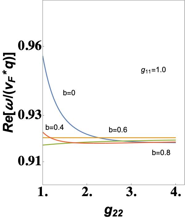
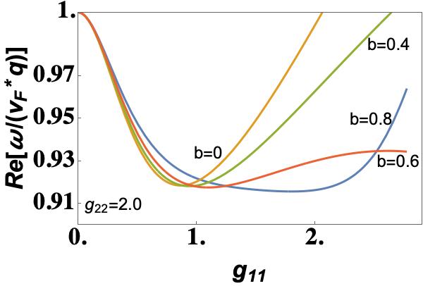
-30pt+65pt

Figure 7: Renormalization of the velocity of the linear dispersion $v_{F}^{*}$ in presence of coupling to high energy correlations. Here we plot the real part of $\omega/(v_{F}^{*}q)$ versus $g_{11}$ at $g_{22}=1.8$ and $v_{F}^{*}q/W=0.1$. Here $g_{12}=b\>g_{11}$ is the coupling strength to the high energy SYK fluctuations ($b=0,0.4,0.6,0.8$, respectively, with $U_{c}/W=10$ and $Z=0.1$).

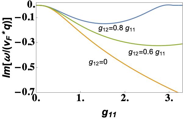
Figure 8: Imaginary part of $\omega/(v_{F}^{*}q)$ versus $g_{11}$ corresponding to the real part of Fig.7 ($g_{12}=bg_{11}$, with $b=0,0.6,0.8$, respectively), at $g_{22}=1.8$ and $v_{F}^{*}q/W=0.1$. Note the flattening at zero for $g_{11}>3.0$, when $b\to 1$.

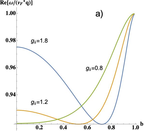
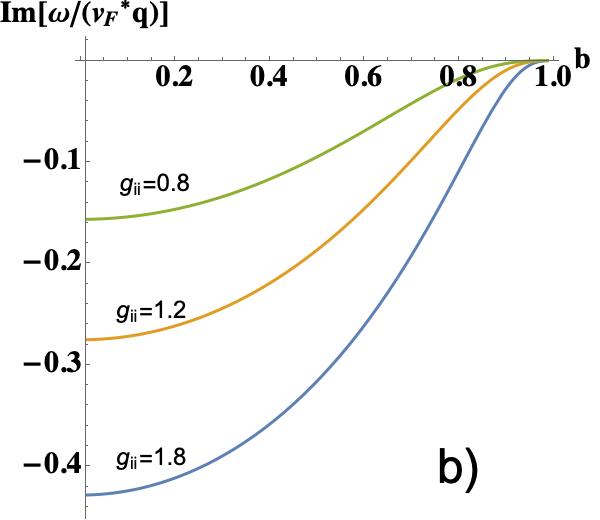
Figure 9: Real [a)] ad Imaginary [b)] part of $\omega/({v}_{F}^{*}q)$ versus $b=g_{12}/g_{11}$ for various values of $g_{ii}\equiv g_{11}=g_{22}$, with $g_{ii}=0.8,1.2,1.8$, respectively, at ${v}_{F}^{*}q/W=0.8$.

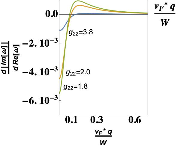
Figure 10: Plot of $\frac{\partial\Im m\{\omega\}}{\partial\Re e\{\omega\}}$ vs ${v}_{F}^{*}q/W$. As $\Re e\{\omega\}$ is strictly linear with $q$ in a large range of values of $q$, the derivative with respect to $\Re e\{\omega\}$ can be interpreted as derivative with respect to $q$. Here $g_{11}=g_{22}=1.8$ and $g_{12}=0.8\times g_{11}$ ($Z=0.1,\>U_{c}/W=10.$, as always)

To sum up the results of this Appendix, we can conclude that the low energy FL on the lattice appears quite robust with respect to interaction with incoherent local disordered SYK clusters, when only the lowest perturbative order is included and no disorder, in the continuum, $k\to 0$, limit. The Fermi surface is still well defined, but the liquid becomes a MFL. The hydrodynamic collective excitation, the would-be acoustic plasmon, is also rather well defined. At strong coupling, in the limit $U_{c}\to{\cal{J}}$, its dispersion tends to the boundary of the p-h continuum and the imaginary part, which blurs the mode, vanishes. We expect that a well defined acoustic plasmon is on the verge to emerge as a bound state at low energies, splitted off the p-h continuum.

Appendix F The superconducting critical temperature at low temperature

In this Appendix we use an EliasbergEliashberg approach to the superconducting critical temperature, $T_{c}$, assuming that pairing is driven by the diffusive excitation modes introduced in Section D. As explained in the main text, $\Omega_{c}^{*}$ is the energy scale of $T_{c}$ and the dependence on the coupling strength turns out to be non BCS-like. We report here the derivation.

In the mean field Hamiltonian, in the NambuNambu (1960) representation,

$$H(k)\equiv\sum_{ij}\>\left[h_{ij}\>\hat{c}^{\dagger}_{i}\>\hat{c}_{j}+\Delta_{ij}c^{\dagger}_{i}c^{\dagger}_{j}+h.c.\right]$$

$$=\sum_{k}\begin{array}[]{c}\left(c_{\vec{k}}\>^{\dagger}\>\>c_{-\vec{k}}\right)\\ \end{array}\>\left(\begin{array}[]{cc}\xi_{k}&\Delta\\ \Delta&-\xi_{k}\end{array}\right)\left(\begin{array}[]{cc}c_{\vec{k}}\\ c_{-\vec{k}}\>^{\dagger}\end{array}\right)$$ (216)

the one electron Green’s function ${\cal{G}}(p,i\>\omega_{\nu})$ and the electronic self-energy $\Sigma(p,i\>\omega_{\nu})$ are $2\times 2$ matrix defined by the Dyson equation

$$\left[{\cal{G}}(p,i\>\omega_{\nu})\right]^{-1}=[G_{0}(p,i\>\omega_{\nu})]^{-1}-\Sigma(p,i\>\omega_{\nu}),$$ (217)

$$=i\>Z^{-1}\omega_{\nu}-\tilde{\xi}_{p}\sigma_{3}-\phi(p,i\>\omega_{\nu})\>\sigma_{1},$$ (218)

where $G_{0}(p,i\>\omega_{\nu})$ is the one-electron Green’ s function for the non interacting system, $\sigma_{i}$ are Pauli matrices and $\xi_{k}=\epsilon_{k}-\mu$. The $\epsilon_{k}$’s are single particle electron energies and $\mu$ is the chemical potential. We do not include Coulomb electron-electron interaction, so that the self-energy $\Sigma\propto\sigma_{1}$ is just offdiagonal. The approximation used for the self-energy is Fiore (2017):

$$\Sigma(p,i\>\omega_{\nu})=-\frac{1}{\beta}\sum_{p^{\prime}\nu^{\prime}}\sigma_{3}\>G(p^{\prime},i\>\omega_{\nu^{\prime}})\>\sigma_{3}\>\left|g(p,\>p^{\prime})\right|^{2}{\cal{D}}\left(p-p^{\prime},i\>\omega_{\nu}-i\>\omega_{\nu^{\prime}}\right),$$ (219)

where $g(p,\>p^{\prime})$ is the coupling with the bosonic modes and ${\cal{D}}\left(p-p^{\prime},i\>\Omega_{n}\right)$ is the response function in imaginary frequency to the bosonic modes. The latter can be represented in terms of its imaginary part, ${\cal{B}}(q,i\>\Omega_{n})=-\frac{1}{\pi}\Im m\left\{{\cal{D}}\left(q,i\>\Omega_{n}\right)\right\}$ as

$${\cal{D}}\left(q,i\>\omega_{\nu}-i\>\omega_{\nu^{\prime}}\right)=\int_{0}^{\infty}d\Omega\>{\cal{B}}(q,\Omega)\left\{\"{\i}\textquestiondown\textonehalf\frac{1}{i\>\omega_{\nu}-i\>\omega_{\nu^{\prime}}-\Omega}-\"{\i}\textquestiondown\textonehalf\frac{1}{i\>\omega_{\nu}-i\>\omega_{\nu^{\prime}}+\Omega}\right\}$$

where ( $\Omega_{q}=\tilde{D}_{Q}q^{2}$ ) and, in our case

$${\cal{B}}(q,i\>\Omega)=-\frac{1}{\pi}\>\left[\frac{\Omega_{q}\>\Omega}{\Omega^{2}+\Omega_{q}^{2}}\right]\>{\cal{T}}_{Q}$$ (220)

To make matches with the usual Eliashberg theory, the isotropic gap model which we consider here provides the dimensionless coupling function :

$$\alpha^{2}F(\Omega)=\!\frac{1}{N_{q}}\!\!\sum_{q}\!\delta(\Omega-\Omega_{q})\nu(0)\!\!\!\int d\omega^{\prime}\left|g(k_{F},\omega^{\prime};q)\right|^{2}\!\!\!,$$ (221)

as an integral over the transferred momentum $q$. We have to integrate over all $q^{\prime}s$:

$$\frac{1}{N_{q}}\>\sum_{q}\quad\quad\mathbf{\Rightarrow}\quad\frac{\tilde{a}^{2}}{(2\pi)^{2}}2\pi\>\int q\frac{d\>q}{d\Omega_{q}}\>d\Omega_{q}=\frac{\tilde{a}^{2}}{2\pi}\frac{1}{2\>\tilde{D}_{Q}}\int d\Omega_{q},$$

where $\tilde{a}^{2}$ is the average diffusion area. We obtain

$$\Sigma(p,i\>\omega_{\nu})=-\frac{1}{\beta}\sum_{p^{\prime}\nu^{\prime}}\sigma_{3}\>{\cal{G}}(p^{\prime},i\>\omega_{\nu^{\prime}})\>\sigma_{3}\>\int d\Omega\frac{1}{4\pi\>}\frac{\tilde{a}^{2}}{\tilde{D}_{Q}}\int d\Omega_{q}\left|g_{p,p^{\prime}}(\Omega_{q})\right|^{2}{\cal{B}}(\Omega_{q},\Omega)\>\left\{\"{\i}\textquestiondown\textonehalf\frac{1}{i\>\omega_{\nu}-i\>\omega_{\nu^{\prime}}-\Omega}-\"{\i}\textquestiondown\textonehalf\frac{1}{i\>\omega_{\nu}-i\>\omega_{\nu^{\prime}}+\Omega}\right\}$$

with

$$\left[{\cal{G}}(p,\omega)\right]^{-1}=Z^{-1}\>{\omega}{\bf 1}-\left\{\xi_{p}-i\>Z^{-1}\left[|\omega|\>\frac{\epsilon_{F}}{\Omega^{*}}\>\ln\left(\frac{{\cal{J}}}{W}\right)+\frac{\alpha}{Z}\>\nu_{0}|\omega|^{2}\>\ln\frac{Z\tilde{v}_{F}k_{F}}{|\omega|}\right]\>sign(\omega)\right\}\sigma_{3}-\Xi(\omega)\sigma_{1}$$ (222)

The mean field $\Delta(\omega)=Z(\omega)\Xi(\omega)$ has to be determined in the following.

In Eq.(222) the inverse lifetime of the quasiparticles of Eq.(68) of MT appears. Here $\alpha$ is a numerical factor of order one.

Note the difference with the usual approach: diffusivity implies Eq.(220) here, while usually is ${\cal{B}}(q,\Omega)\sim\frac{\Omega_{q}}{\Omega_{q}^{2}+\Omega^{2}}$ in the Eliashberg approach.

On the other hand, from Eq.(217): The final form of the selfenergy is:

$$\Sigma(p,\omega)=\nu_{0}\int_{-\infty}^{\infty}d\omega^{\prime}\>\Re e\left\{\frac{Z^{-1}\omega^{\prime}{\bf 1}-\Xi(\omega^{\prime})\>\sigma_{1}}{\left[{\cal{P}}(\omega^{\prime})\right]^{1/2}}\right\}\>\int_{0}^{\infty}d\Omega\int\frac{d\Omega_{q}}{4\pi}\left|g_{p,p^{\prime}}(\Omega_{q})\right|^{2}{\cal{B}}(\Omega_{q},\Omega)$$

$$\times\left[\frac{f(-\omega^{\prime})}{\omega-\omega^{\prime}-\Omega+i\>0^{+}}+\frac{f(\omega^{\prime})}{\omega-\omega^{\prime}+\Omega+i\>0^{+}}+\frac{N(\Omega)}{\omega-\omega^{\prime}-\Omega+i\>0^{+}}+\frac{N(\Omega)}{\omega-\omega^{\prime}+\Omega+i\>0^{+}}\right],$$

$${\cal{P}}(\omega)=Z^{-2}\>{\omega}^{2}+Z^{-2}\>\left[|\omega|\>\frac{\epsilon_{F}}{\Omega^{*}}\>\ln\left(\frac{{\cal{J}}}{W}\right)+\frac{\alpha}{Z}\>\nu_{0}|\omega|^{2}\>\ln\frac{Z\tilde{v}_{F}k_{F}}{|\omega|}\right]^{2}-\Xi^{2}(\omega),$$ (223)

where $N(\Omega)=\left[e^{\beta\Omega}-1\right]^{-1}$ and $f(\omega)=\left[e^{\beta\omega}+1\right]^{-1}$ are the Bose and Fermi occupation probabilities. The term in curly brackets arises from $\Im m\left\{\nu_{0}\int_{-\infty}^{+\infty}d\xi_{p^{\prime}}\>\sigma_{3}{\cal{G}}(p^{\prime},\omega)\>\sigma_{3}\right\}$, which turns into a real part from the inverse of $\left[{\cal{G}}(p^{\prime},\omega)\right]^{-1}$ given in Eq.(222). The critical temperature is the one at which $\Delta\sim 0$ and can be dropped in the denominator, but the gap equation has to be satisfied.

In all the further calculations we neglect the thermal excitations and drop $N(\Omega)$. Observing that the integration variable $\Omega_{q}$ has the meaning of the diffusive energy (see Eq.(220)) it is clear that it cannot be integrated at energies above $\Omega$. We also use the parameter equality $Z\nu_{0}=U_{c}^{-1}$ and we take $\left|g_{k_{F},\omega^{\prime}}(\Omega_{q})\right|^{2}=g^{2}$ constant ($[g]^{-1}\sim\>time\>\>(\hbar=1\>$ here)). We get:

$$\Delta(\omega)\approx\frac{\tilde{a}^{2}}{\tilde{D}_{Q}}\int_{0}^{\infty}\frac{d\omega^{\prime}}{|\omega^{\prime}|\>\frac{U_{c}\epsilon_{F}}{W^{2}}\>\ln\left(\frac{U_{c}}{W}\right)}\>\Re e\left\{\Delta(\omega^{\prime})\right\}\>\>\frac{1}{U_{c}}\int_{0}^{U_{c}}d\Omega$$

$$\times\int_{0}^{\Omega}\frac{d\Omega_{q}}{4\pi}\left|g_{k_{F},\omega^{\prime}}(\Omega_{q})\right|^{2}\left(\frac{1}{\pi}\>\left[\frac{\Omega_{q}\>\Omega}{\Omega^{2}+\Omega_{q}^{2}}\right]\>{\cal{T}}_{Q}\right)\>2\left\{f(-\omega^{\prime})\frac{1}{\Omega+\omega^{\prime}}-f(\omega^{\prime})\frac{1}{\Omega-\omega^{\prime}}\right\}.$$ (224)

We concentrate on $\omega=0$ and we deal with two contributions to $\Delta(\omega^{\prime})$ separately, $\Delta(\omega^{\prime})=\Delta_{a}+\Delta_{b}$, where the first arises from integration over $0<\omega^{\prime}<\Omega^{*}\sim W^{2}/U_{c}$ and the second from integration over $\Omega^{*}<\omega^{\prime}<U_{c}$.

In the first case, observing that the range of $\omega^{\prime}$ cannot be larger than $\Omega^{*}$, but the Fermi function selects $\omega^{\prime}\sim 0$, we neglect $\omega^{\prime}$ in the denominators of the curly bracket obtaining Tinkham (2004):

$$\Delta_{a}(0)=\frac{\tilde{a}_{\ell}^{2}}{\tilde{D}_{Q}}\int_{0}^{\Omega^{*}}d\omega^{\prime}\>\frac{\Delta_{o}}{\omega^{\prime}\>\frac{\epsilon_{F}}{\Omega^{*}}\>\ln\left(\frac{{\cal{J}}}{W}\right)}\>\>\frac{|g|^{2}\ln 2}{4\>U_{c}}\int_{0}^{U_{c}}\frac{d\Omega}{2\pi}\>\>{\cal{T}}_{Q}\left\{f(-\omega^{\prime})-f(\omega^{\prime})\right\}$$

$$\approx\frac{\tilde{a}_{\ell}^{2}}{\tilde{D}_{Q}}{\cal{T}}_{Q}\>\frac{|g|^{2}\ln 2}{8\pi}\frac{\Delta_{o}}{\frac{\epsilon_{F}}{\Omega^{*}}\>\ln\left(\frac{{\cal{J}}}{W}\right)}\>\int_{0}^{\Omega^{*}}\frac{d\omega^{\prime}}{\omega^{\prime}}\>\tanh\frac{\beta\omega^{\prime}}{2}\approx\frac{\tilde{a}_{\ell}^{2}}{\tilde{D}_{Q}}{\cal{T}}_{Q}\>\frac{|g|^{2}\ln 2}{8\pi}\frac{\Delta_{o}}{\frac{\epsilon_{F}}{\Omega^{*}}\>\ln\left(\frac{{\cal{J}}}{W}\right)}\>\ln{\beta_{c}\Omega^{*}}.$$

Now the $\Delta_{b}$ contribution. We neglect $\Omega$ in the denominator in the curly bracket of Eq.(224) and we include the ${\omega^{\prime}}^{2}$ term of the inverse lifetime, only.

$$\Delta_{b}(0)=\frac{\tilde{a}^{2}}{\tilde{D}_{Q}}\int^{U_{c}}_{\Omega_{c}^{*}}d\omega^{\prime}\>\frac{\Delta_{\infty}}{\frac{\alpha}{Z}\>\nu_{0}|\omega^{\prime}|^{2}\>\ln\frac{Z\tilde{v}_{F}k_{F}}{|\omega^{\prime}|}}\>\>\frac{1}{U_{c}}\int_{0}^{U_{c}}d\Omega\int_{0}^{\Omega}\frac{d\Omega_{q}}{4\pi}\left|g_{k_{F},\omega^{\prime}}(\Omega_{q})\right|^{2}$$

$$\times\left(\frac{1}{\pi}\>\left[\frac{\Omega_{q}\>\Omega}{\Omega^{2}+\Omega_{q}^{2}}\right]\>{\cal{T}}_{Q}\right)\>2\left\{f(-\omega^{\prime})\frac{1}{\Omega+\omega^{\prime}}-f(\omega^{\prime})\frac{1}{\Omega-\omega^{\prime}}\right\}$$

$$=\frac{\tilde{a}^{2}}{\tilde{D}_{Q}}\>\frac{|g|^{2}\ln 2}{4\pi^{2}}\>{\cal{T}}_{Q}\>\int^{U_{c}}_{\Omega_{c}^{*}}d\omega^{\prime}\>\frac{\Delta_{\infty}}{\frac{\alpha}{Z}\>\nu_{0}|\omega^{\prime}|^{2}\>\ln\frac{Z\tilde{v}_{F}k_{F}}{|\omega^{\prime}|}}\>\>\frac{1}{U_{c}}\int_{0}^{U_{c}}2\Omega\>d\Omega\>\frac{1}{\Omega+\omega^{\prime}}$$

where we have disregarded the terms $\propto e^{-\beta\omega^{\prime}}$ in the last integral. The rest of the derivation can be found in the main text.

References

- Hill et al. (2001) R. W. Hill, C. Proust, L. Taillefer, P. Fournier, and R. L. Greene, Nature 414, 711 (2001), URL https://doi.org/10.1038/414711a.
- Jain and Anderson (2009) J. K. Jain and P. W. Anderson, Proceedings of the National Academy of Sciences 106, 9131 (2009), ISSN 0027-8424, eprint https://www.pnas.org/content/106/23/9131.full.pdf, URL https://www.pnas.org/content/106/23/9131.
- Chowdhury and Berg (2020a) D. Chowdhury and E. Berg, Phys. Rev. Research 2, 013301 (2020a), URL https://link.aps.org/doi/10.1103/PhysRevResearch.2.013301.
- Lantagne-Hurtubise et al. (2021) E. Lantagne-Hurtubise, V. Pathak, S. Sahoo, and M. Franz, arXiv:2012.12491 (2021).
- Sachdev and Ye (1993) S. Sachdev and J. Ye, Phys. Rev. Lett. 70, 3339 (1993).
-
(6)
A. Kitaev,
A simple model of quantum holography,
entanglement in StronglyCorrelated Quantum Matter - KITP
Program 2015,
URL https://online.kitp.ucsb.edu/online/entangled15/kitaev/
https://online.kitp.ucsb.edu/online/entangled15/kitaev2/. - Kitaev and Suh (2018) A. Kitaev and S. J. Suh, Journal of High Energy Physics 2018, 183 (2018), ISSN 1029-8479.
- Maldacena and Stanford (2016) J. Maldacena and D. Stanford, Phys. Rev. D 94, 106002 (2016).
- Sachdev (2010) S. Sachdev, Phys. Rev. Lett. 105, 151602 (2010), URL https://link.aps.org/doi/10.1103/PhysRevLett.105.151602.
- Diaz et al. (2018) P. Diaz, S. Das, and M. Walton, International Journal of Modern Physics D 27, 1850090 (2018).
- Gu et al. (2017) Y. Gu, X.-L. Qi, and D. Stanford, Journal of High Energy Physics 2017, 125 (2017), ISSN 1029-8479, URL https://doi.org/10.1007/JHEP05(2017)125.
- Davison et al. (2017) R. A. Davison, W. Fu, A. Georges, Y. Gu, K. Jensen, and S. Sachdev, Phys. Rev. B 95, 155131 (2017), URL https://link.aps.org/doi/10.1103/PhysRevB.95.155131.
- Song et al. (2017) X.-Y. Song, C.-M. Jian, and L. Balents, Phys. Rev. Lett. 119, 216601 (2017), URL https://link.aps.org/doi/10.1103/PhysRevLett.119.216601.
- Berkooz et al. (2017) M. Berkooz, P. Narayan, M. Rozali, and J. Simón, Journal of High Energy Physics 2017, 138 (2017), ISSN 1029-8479.
- Chew et al. (2017) A. Chew, A. Essin, and J. Alicea, Phys. Rev. B 96, 121119 (2017), eprint 1703.06890.
- Haldar and Shenoy (2018) A. Haldar and V. B. Shenoy, Phys. Rev. B 98, 165135 (2018).
- Patel et al. (2018a) A. A. Patel, J. McGreevy, D. P. Arovas, and S. Sachdev, Phys. Rev. X 8, 021049 (2018a), URL https://link.aps.org/doi/10.1103/PhysRevX.8.021049.
- Chowdhury et al. (2018) D. Chowdhury, Y. Werman, E. Berg, and T. Senthil, Phys. Rev. X 8, 031024 (2018), URL https://link.aps.org/doi/10.1103/PhysRevX.8.031024.
- Parcollet and Georges (1999) O. Parcollet and A. Georges, Phys. Rev. B 59, 5341 (1999), URL https://link.aps.org/doi/10.1103/PhysRevB.59.5341.
- Varma et al. (2002) C. Varma, Z. Nussinov, and W. van Saarloos, Physics Reports 361, 267 (2002), ISSN 0370-1573, URL http://www.sciencedirect.com/science/article/pii/S0370157301000606.
- Ben-Zion and McGreevy (2018) D. Ben-Zion and J. McGreevy, Phys. Rev. B 97, 155117 (2018).
- Patel et al. (2018b) A. A. Patel, M. J. Lawler, and E.-A. Kim, Phys. Rev. Lett. 121, 187001 (2018b), URL https://link.aps.org/doi/10.1103/PhysRevLett.121.187001.
- Gurvitch and Fiory (1987) M. Gurvitch and A. T. Fiory, Phys.Rev.Lett. 59, 1337 (1987).
- Daou et al. (2008) R. Daou, N. Doiron-Leyraud, D. LeBoeuf, S. Li, F. Laliberté, O. Cyr-Choiniére, Y. Jo, L. Balicas, J.-Q. Yan, J.-S. Zhou, et al., Nature Physics 5, 31 (2008).
- Cha et al. (2020a) P. Cha, N. Wentzell, O. Parcollet, A. Georges, and E.-A. Kim, Proceedings of the National Academy of Sciences 117, 18341 (2020a), ISSN 0027-8424, eprint https://www.pnas.org/content/117/31/18341.full.pdf, URL https://www.pnas.org/content/117/31/18341.
- Kitaev (2018) A. Kitaev, Notes on representations (2018), eprint 1711.08169.
- Bunkov and Volovik (2009) Y. M. Bunkov and G. E. Volovik, Magnon BEC and Spin Superfluidity: a 3He primer (2009), eprint 0904.3889.
- Zhang (2017) P. Zhang, Phys. Rev. B 96, 205138 (2017).
- Fu and Sachdev (2016) W. Fu and S. Sachdev, Phys. Rev. B 94, 035135 (2016), URL https://link.aps.org/doi/10.1103/PhysRevB.94.035135.
- Cha et al. (2020b) P. Cha, A. A. Patel, E. Gull, and E.-A. Kim, Phys. Rev. Research 2, 033434 (2020b), URL https://link.aps.org/doi/10.1103/PhysRevResearch.2.033434.
- Klebanov et al. (2020) I. Klebanov, A. Milekhin, G. Tarnopolsky, and et al, J. High Energ. Phys. 2020, 162 (2020).
- Tagliacozzo (2021) A. Tagliacozzo, arXiv:2106.05383 (2021), URL https://arxiv.org/abs/2106.05383.
- Akkermans and Montambaux (2007) E. Akkermans and G. Montambaux, Mesoscopic Physics of Electrons and Photons (Cambridge University Press, 2007).
- Hartnoll (2015) S. A. Hartnoll, Nature Physics 11, 54 (2015).
- Haldar et al. (2018) A. Haldar, S. Banerjee, and V. B. Shenoy, Phys. Rev. B 97, 241106 (2018).
- Khveshchenko (2018) D. V. Khveshchenko, SciPost Phys. 5, 12 (2018).
- mar (2020) Annals of Physics 417, 168102 (2020), ISSN 0003-4916, eliashberg theory at 60: Strong-coupling superconductivity and beyond.
- Chowdhury and Berg (2020b) D. Chowdhury and E. Berg, Annals of Physics 417, 168125 (2020b), ISSN 0003-4916, URL http://www.sciencedirect.com/science/article/pii/S0003491620300580.
- (39) Checking : Green’s function has a with so that . . because .
- Negele and Orland (1987) J. Negele and H. Orland, Quantum Many-Particle Systems (Addison Wesley Publishing Company, 1987).
- Chakravarty and Leggett (1984) S. Chakravarty and A. Leggett, Physical Review Letters 52 (1984).
- Roman (1969) P. Roman, Introduction to Quantum Field Theory (Wiley - 1st Ed., 1969).
- Kamenev and Levchenko (2009) A. Kamenev and A. Levchenko, Advances in Physics 58, 197 (2009), eprint https://doi.org/10.1080/00018730902850504, URL https://doi.org/10.1080/00018730902850504.
- Kovtun et al. (2005) P. K. Kovtun, D. T. Son, and A. O. Starinets, Phys. Rev. Lett. 94, 111601 (2005).
- (45) G. M. Eliashberg (????).
- McMillan (1968) W. L. McMillan, Phys. Rev. 167, 331 (1968).
- Tinkham (2004) M. Tinkham, Introduction to Superconductivity (Dover Publications, 2004), 2nd ed.
- Lavasani et al. (2019) A. Lavasani, D. Bulmash, and S. Das Sarma, Phys. Rev. B 99, 085104 (2019).
- Carlson et al. (2002) E. W. Carlson, V. J. Emery, S. A. Kivelson, and D. Orgad, Concepts in high temperature superconductivity (2002), eprint 0206217.
- Sreedhar et al. (2020) S. A. Sreedhar, A. Rossi, J. Nayak, Z. W. Anderson, Y. Tang, B. Gregory, M. Hashimoto, D.-H. Lu, E. Rotenberg, R. J. Birgeneau, et al., Phys. Rev. B 102, 205109 (2020).
- Ye (1998) J. Ye, Phys. Rev. B 58, 9450 (1998).
- Shekhter and Varma (2009) A. Shekhter and C. M. Varma, Phys. Rev. B 79, 045117 (2009).
- Lee (2014) P. A. Lee, Phys. Rev. X 4, 031017 (2014), URL https://link.aps.org/doi/10.1103/PhysRevX.4.031017.
- Kopnický and Hlubina (2020) L. c. v. Kopnický and R. Hlubina, Phys. Rev. B 101, 024502 (2020), URL https://link.aps.org/doi/10.1103/PhysRevB.101.024502.
- Schrieffer (1995) J. R. Schrieffer, Journal of Low Temperature Physics 99, 397 (1995), ISSN 1573-7357.
- Babaev and Speight (2005) E. Babaev and M. Speight, Phys. Rev. B 72, 180502 (2005), URL https://link.aps.org/doi/10.1103/PhysRevB.72.180502.
- Silaev and Babaev (2012) M. Silaev and E. Babaev, Phys. Rev. B 85, 134514 (2012), URL https://link.aps.org/doi/10.1103/PhysRevB.85.134514.
- Ernst Helmut Brandt and Das (2011) E. Ernst Helmut Brandt and M. P. Das, J Supercond Nov Magn 24, 57 (2011).
- Kogan and Schmalian (2012) V. G. Kogan and J. Schmalian, Phys. Rev. B 86, 016502 (2012).
- Babaev and Silaev (2012) E. Babaev and M. Silaev, Phys. Rev. B 86, 016501 (2012), URL https://link.aps.org/doi/10.1103/PhysRevB.86.016501.
- Belzig et al. (1999) W. Belzig, F. K. Wilhelm, C. Bruder, G. Schon, and A. D. Zaikin, Superlattices and Microstructures 25, 1251 (1999), ISSN 0749-6036, URL http://www.sciencedirect.com/science/article/pii/S0749603699907103.
- Wen (2010) X.-G. Wen, Quantum Field Theory of Many-Body Systems (Oxford University Press Inc, 2010).
- Abramowitz and Stegun (1970) M. Abramowitz and I. A. Stegun, Handbook of Mathematical Functions (Dover Publications, 1970).
- Pientka et al. (2017) F. Pientka, J. Waissman, P. Kim, and B. I. Halperin, Phys. Rev. Lett. 119, 027601 (2017), URL https://link.aps.org/doi/10.1103/PhysRevLett.119.027601.
- Alexander L. Fetter (2003) J. D. W. Alexander L. Fetter, Quantum Theory of Many-Particle Systems (Dover Publications, 2003).
- Ashcroft and Mermin (1976) N. W. Ashcroft and N. D. Mermin, Solid State Physics (Brooks Cole, 1976), 1st ed.
- Nambu (1960) Y. Nambu, Phys. Rev. 117, 648 (1960), URL https://link.aps.org/doi/10.1103/PhysRev.117.648.
- Fiore (2017) S. Fiore, Master’s thesis, Universita’ di Napoli, "Federico II", Napoli (2017).