Design of borehole resistivity measurement acquisition systems using deep learning

Abstract

Borehole resistivity measurements recorded with logging-while-drilling (LWD) instruments are widely used for characterizing the earth’s subsurface properties. They facilitate the extraction of natural resources such as oil and gas. LWD instruments require real-time inversions of electromagnetic measurements to estimate the electrical properties of the earth’s subsurface near the well and possibly correct the well trajectory.

Deep Neural Network (DNN)-based methods are suitable for the rapid inversion of borehole resistivity measurements as they approximate the forward and inverse problem offline during the training phase and they only require a fraction of a second for the evaluation (aka prediction). However, the inverse problem generally admits multiple solutions. DNNs with traditional loss functions based on data misfit are ill-equipped for solving an inverse problem. This can be partially overcome by adding regularization terms to a loss function specifically designed for encoder-decoder architectures. But adding regularization seriously limits the number of possible solutions to a set of a priori desirable physical solutions. To avoid this, we use a two-step loss function without any regularization [1].

In addition, to guarantee an inverse solution, we need a carefully selected measurement acquisition system with a sufficient number of measurements. In this work, we propose a DNN-based iterative algorithm for designing such a measurement acquisition system. We illustrate our DNN-based iterative algorithm via several synthetic examples. Numerical results show that the obtained measurement acquisition system is sufficient to identify and characterize both resistive and conductive layers above and below the logging instrument. Numerical results are promising, although further improvements are required to make our method amenable for industrial purposes.

Keywords: logging-while-drilling (LWD), resistivity measurements, real-time inversion, deep learning, well geosteering, deep neural networks, measurement acquisition system.

1 Introduction

One of the motivations for the geophysical exploration of the earth’s subsurface is to facilitate the extraction of natural resources such as oil and gas. Other applications include geothermal exploration and CO₂-sequestration. To this end, there exist a wide variety of techniques intended to estimate different subsurface properties. Here, we focus on resistivity measurements [2, 3], which intend to determine electrical resistivity (and sometimes dielectric permittivity) of subsurface materials.

We characterize resistivity measurements depending on the acquisition location as: a) on the surface, which includes those acquired with controlled source electromagnetic (CSEM) [4, 5, 6, 7, 8] and magnetotellurics (MT) [9]; and b) in the borehole, often recorded with logging while drilling (LWD) devices [10, 11]. In this work, we focus on borehole resistivity measurements recorded with LWD instruments.

In LWD, a well logging tool conveys down into the well borehole, records electromagnetic measurements and transmits the data in real-time to evaluate the formation and subsequently adjust the inclination and azimuth of the well trajectory [12]. This strategy to determine a well trajectory is known as geosteering and it is crucial for maximizing the extraction of oil and gas.

The main challenge when dealing with geosteering is the need to interpret borehole resistivity measurements rapidly, i.e., we need to invert these measurements in real-time. Traditional inversion methods are often computationally expensive [13, 14]. For example, gradient-based methods [15, 13] require simulating the forward problem dozens of times per logging positions. These methods need to evaluate derivatives of measurements with respect to the inversion variables, which is often challenging and time-consuming [13, 14]. An alternative to gradient-based techniques is to apply statistics-based methods [15, 13, 16], which search for a global minima rather than a local one. However, these methods aggravate the problem of high computation time since these techniques often require a large number of forward simulations. Moreover, for each new set of measurements, i.e., for each logging position, one needs to repeat the entire inversion process, which could be computationally intensive.

These difficulties can be partially overcome by using deep neural networks (DNNs), as shown in recent works [17, 1, 18]. While DNNs involve generating a large dataset for the training of the neural network, the biggest advantage of DNN methods is that they approximate the forward and inverse problem offline. Once the training process is completed, online prediction (evaluation) takes a fraction of a second. This makes DNN methods powerful candidates for real-time inversion [17, 1]. Unlike gradient-based and statistics-based methods, DNN methods do not require the solution of the forward problem after recording each new set of measurements.

For two and three-dimensional earth subsurface models, we need to employ numerical techniques such as the finite element method (FEM) [19, 4, 9], the finite volume (FV) [20], or the finite difference method (FDM) [10, 21, 22] to solve the forward problem. Thus, producing a dataset for DNNs may lead to prohibitively expensive computational costs. We can lower the costs by restricting to $1$D layered earth models [23]. In multiple realistic scenarios, $1$D earth models approximate the geological earth formation reasonably well, and it is often used for borehole resistivity inversion in the oil and gas industry. This technique takes small simulation time (typically, a fraction of a second) due to the availability of a semi-analytical method [24]. In this work, we restrict to 1D earth models for the sake of computational efficiency, although the method proposed here can be easily extended to 2D and 3D, provided sufficient computational resources are available.

As illustrated in [1], DNNs equipped with a traditional loss function based on the data misfit exhibit serious limitations when predicting some physically realistic solutions to the inverse problems. Such limitations occur because inverse problems often admit multiple solutions. The performance of a DNN for solving an inverse problem could be drastically improved with a loss function specifically designed for encoder-decoder architectures or a two-step loss function [1]. Regularization terms added to the loss function can guide the solution towards an a priori “desirable” physical solution; however, they often hide the fact that other “physical” solutions may also co-exist [1].

Herein, we consider the two-step loss function based on the measurement misfit described in [1] without regularization terms. The main advantage of this choice is that we can recover all possible solutions of the inverse problem (in the sense that they satisfy the measurements), and not simply those dictated by the regularization term. This opens the door to analyze how many inverse solutions satisfy all measurements of a given measurement acquisition system. Alternatively, we can enrich the measurement acquisition system until guaranteeing that the inverse solution is unique. This is the approach we take in this work.

The main goal of the present work is to design a measurement acquisition system that guarantees a solution of practical interest. For that purpose, we propose a DNN-based iterative method. We start by considering a large set of borehole logging resistivity measurements from which we first select a single one. Then, we iteratively add a new measurement such that it minimizes the number of existing inverse solutions. To select the new measurement in each step of the iterative algorithm, we employ the coefficient of determination (also known as $R^{2}$ or $R$-squared statistic) [25].

In the following, we describe a DNN-based algorithm for designing a measurement acquisition system, and we illustrate its performance with several synthetic examples, analyzing its benefits and limitations. Improvement of some technical aspects such as optimal data sampling techniques and selection of DNN architecture [26, 14] can make the DNN-based inversion method more robust. However, for simplicity, we do not analyze those aspects here. We neither consider noisy measurements, which will be the subject of future work.

The remainder of this paper is organized as follows. Section 2 provides an abstract formulation of the problem. Section 3 describes the deep learning algorithm used in this work. Section 4 details the measuring devices, measured components, and data space. Section 5 discusses the algorithm for designing the measurement acquisition system. The numerical implementation is discussed in Section 6. Section 7 demonstrates the applicability of our method with some examples. Section 8 is devoted to conclusions and a brief discussion including possible future work.

2 Problem formulation

We introduce two different mathematical problems associated with borehole resistivity measurements: forward and inverse (see Figure 1).

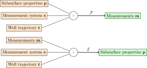
Figure 1: Schematic diagram of a forward and an inverse problem.

Forward problem.

Given an earth model $\mathbf{p}\in\mathbb{R}^{n_{p}}$, a well trajectory $\mathbf{t}\in\mathbb{R}^{n_{t}}$ and a measurement acquisition system $\mathbf{s}\in\mathbb{R}^{n_{s}}$, the forward problem $\cal F$ delivers the corresponding measurements $\mathbf{m}({\mathbf{s}})\in\mathbb{R}^{n_{m}}$; the variables are parameterized by real-valued vectors with $n_{(\cdot)}$ dimensions. Mathematically, we have:

$${\mathcal{F}}({\mathbf{s}},{\mathbf{t}},{\mathbf{p}}) ={\mathbf{m}}({\mathbf{s}})\quad\text{(Forward)}.$$ (1)

The forward operator $\cal F$ is governed by partial differential equations (PDEs), in this case, Maxwell’s equations in the frequency domain with the corresponding boundary conditions governing the electromagnetic wave propagation phenomena [19].

Inverse problem.

Given a set of measurements $\mathbf{m}$ obtained with a specific measurement acquisition system $\mathbf{s}$ and logging trajectory $\mathbf{t}$, the inverse operator $\cal{I}$ determines a plausible earth model $\mathbf{p}$, in the sense that it satisfies the recorded measurements. The earth model is characterized by a material subsurface distribution. We have:

$$\mathcal{I}({\mathbf{s}},{\mathbf{t}},{\mathbf{m}}({\mathbf{s}})) ={\mathbf{p}},\quad\text{(Inverse)}$$ (2)

An inverse problem often exhibits multiple solutions [13, 15] since different earth models may satisfy the recorded measurements.

Earth parametrization.

We restrict to a $1$D layered model of the earth. This assumption is common for geosteering applications [7, 11] since it allows to simulate a problem in a fraction of a second using a semi-analytic method [23, 19]. We further assume the earth model to be a three-layer medium [24], as illustrated in Figure 2. This medium is generally characterized by seven parameters, namely:

1. Horizontal resistivity $\rho_{h}$ of the layer containing the mid-point of the logging instrument.

2. Vertical resistivity $\rho_{v}$ of of the layer containing the mid-point of the logging instrument. Often, instead of two different resistivities, $\rho_{v}$ is replaced by anisotropy factor $a$, i.e. $\frac{\rho_{v}}{\rho_{h}}$.

3. The resistivity of the layer located below the current layer $\rho_{l}$.

4. The resistivity of the layer located above the current layer $\rho_{u}$.

5. Vertical distance from the current logging position to the upper bed boundary $d_{u}$.

6. Vertical distance from the current logging position to the lower bed boundary $d_{l}$.

7. The dip angle ($\beta$) of the formation.

In this work, for simplicity, we assume earth model $E_{5}\mathrel{\mathop{\mathchar 58\relax}}=\{\rho_{v},~{}\rho_{l},~{}\rho_{u},~{}d_{u},~{}d_{l}\}$, i.e., we assume isotropic formations $\rho_{h}=\rho_{v}$ and formation dip angle $\beta=0$. However, our algorithm for designing measurement acquisition systems can be applied to other earth parameterizations.

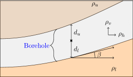
Figure 2: 1D media and a trajectory. The black circle indicates the current position of the midpoint of the logging instrument.

3 Deep learning loss function

We briefly describe here the deep learning approach adopted for this work. The interested reader can find a more detailed discussion on other deep learning algorithms in books (e.g [27]) and review articles ( e.g. [28]).

Our target is to approximate the inverse operator $\mathcal{I}\mathrel{\mathop{\mathchar 58\relax}}~{}\mathbb{R}^{n_{s}}\times\mathbb{R}^{n_{t}}\times\mathbb{R}^{n_{m}}\mapsto\mathbb{R}^{n_{p}}$ using a DNN. After the model architecture is created, we optimize a loss function to train our DNN. The simplest loss function is based on data misfit and optimized in $l_{1}$ or $l_{2}$ norm, given by:

$$\mathcal{I}_{\alpha^{\ast}} \mathrel{\mathop{\mathchar 58\relax}}=\arg\min_{\alpha}\mathinner{\!\left\lVert\mathcal{I}_{\alpha}(\mathbf{s},\mathbf{t},\mathbf{m})-\mathbf{p}\right\rVert},$$ (3)

where $\alpha$ is the set of weights associated to the DNN.

However, due to the non-uniqueness of the solution in inverse problems, this loss function produces an average of various plausible solutions. Hence, it may produce incorrect results in the sense that the forward simulation of the average of several solutions may not satisfy the measurements [1].

We can overcome this limitation by optimizing a loss function based on the misfit of measurements [29], given by:

$$\mathcal{I}_{\alpha^{\ast}}\mathrel{\mathop{\mathchar 58\relax}}=\arg\min_{\alpha}\mathinner{\!\left\lVert(\mathcal{F}\circ\mathcal{I}_{\alpha})(\mathbf{s},\mathbf{t},\mathbf{m})-\mathbf{m}\right\rVert},$$ (4)

where $\alpha$ is the set of weights associated to the DNN.

Although the above loss function produces accurate results, it has some critical limitations [1]. First, the requirement of evaluating the forward problem multiple times during training may result in a prohibitively high computational time. Second, although sophisticated and GPU-compatible libraries like Tensorflow [30] are available for training of a DNN, the forward problem is generally solved in a CPU. This produces a communication bottleneck between CPU and GPU. We can remove this bottleneck by making the forward solver GPU-compatible, but this involves additional implementation challenges.

A suitable alternative is to solve the following optimization problem [1]:

$$({\cal F}_{\alpha^{\ast}},\mathcal{I}_{\beta^{\ast}})\mathrel{\mathop{\mathchar 58\relax}}=\arg\min_{\alpha,\beta}\big{(} \mathinner{\!\left\lVert(\mathcal{F}_{\alpha}\circ\mathcal{I}_{\beta})(\mathbf{s},\mathbf{t},\mathbf{m})-\mathbf{m}\right\rVert}+\mathinner{\!\left\lVert\mathcal{F}_{\alpha}(\mathbf{s},\mathbf{t},\mathbf{p})-\mathbf{m}\right\rVert}\big{)},$$ (5)

where $\alpha$ and $\beta$ are the set of weights associated to the DNNs which we use to approximate the forward function and inverse operator respectively.

The above loss function consists of two terms. The first one constitutes an encoder-decoder architecture [31] and ensures that $\mathcal{I}_{\beta}$ is an inverse of $\mathcal{F}_{\alpha}$. The second one guarantees that the forward DNN approximates the measurements.

We can also split the previous minimization problem into two steps [1]. In the first step, we approximate the forward operator:

$${\cal F}_{\alpha^{\ast}}(\mathbf{s})\mathrel{\mathop{\mathchar 58\relax}}=\arg\min_{\alpha}\mathinner{\!\left\lVert{\cal F}_{\alpha}(\mathbf{s},\mathbf{t},\mathbf{p})-\mathbf{m}({\mathbf{s}})\right\rVert}.$$ (6)

Next, we determine the inverse operator:

$${\cal I}_{\beta^{\ast}}(\mathbf{s})\mathrel{\mathop{\mathchar 58\relax}}=\arg\min_{\beta}\mathinner{\!\left\lVert({\cal F}_{\alpha^{\ast}}\circ{\cal I}_{\beta})(\mathbf{s},\mathbf{t},\mathbf{m}({\mathbf{s}}))-\mathbf{m}({\mathbf{s}})\right\rVert}.$$ (7)

We use this two-step approach for our deep learning algorithm.

Remark.

In the above expressions, $\mathinner{\!\left\lVert\cdot\right\rVert}$ denotes some suitable matrix norm. For details, see [1].

4 Databases with multiple measurements

4.1 Borehole resistivity measurements

Logging instrument.

Modern borehole resistivity instruments can measure all possible (nine) couplings of the magnetic field $H_{ij}$, where $i$ indicates the orientation of the transmitter and $j$ stands for the receiver orientation. We obtain different measurements combining one or more $H_{ij}$. The measurements further depend on the number and locations of the transmitters and receivers along the logging instrument. We consider two different types of logging instruments:

1. Conventional LWD. We consider an instrument that incorporates a pair of receivers and three pairs of transmitters, as illustrated in Figure 3. We refer to them as short-spaced, medium-spaced, and long-spaced depending on the distance to the receiver. In this case, each measurement is specified by a pair of transmitters, a specific operator frequency, and the pair of receivers (Table 1).

   

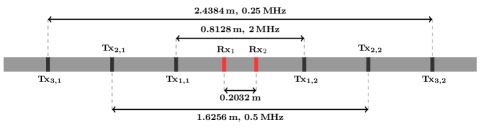
   Figure 3: Conventional LWD. Tx_i,j, j=1,2 denote the transmitters and i=1,2,3 specifies the spacing between the transmitters. Rx₁, Rx₂ stands for the two receivers.

2. A deep azimuthal instrument. We consider an instrument that incorporates one transmitter that can operate at two different frequencies and two associated receivers, as depicted in Figure 4. Using a deep azimuthal instrument, each measurement is specified by the transmitter with an operating frequency and the corresponding receiver (Table 1).

   

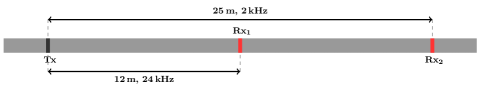
   Figure 4: Deep azimuthal instrument. It has one transmitter Tx operating at two different frequencies and two receivers Rx₁, Rx₂.

   Measurement Systems	$n_{T}$	$n_{R}$	Spacing	$p_{T}~{}[$\mathrm{m}$]$	$p_{R}~{}[$\mathrm{m}$]$	$\nu~{}[$\mathrm{kHz}$]$
   Conventional LWD	$6$	$2$	short	$\pm 0.4064$	$\pm 0.1016$	2000
   			medium	$\pm 0.8128$	$\pm 0.1016$	500
   			long	$\pm 1.2192$	$\pm 0.1016$	250
   Deep azimuthal instrument	$1$	$2$	short	$-12.0$	$0.0$	$24$
   			long	$-12.0$	$13.0$	$2$

   Table 1: Different measurement systems and their configurations. We list here the number of transmitters $n_{T}$ and receivers $n_{R}$, the positions of the transmitters ($p_{T}$) and the receivers ($p_{R}$), and the frequency of the emitted pulse ($\nu$).

Measured component.

We record certain components of the electromagnetic field with different instruments, as listed in Table 2. Measurement logs vary depending on the number of receivers and transmitters [17].

Let $m_{c}$ be a measured component. When using a conventional LWD instrument, we record $m_{c}$ at both receivers (and denote it as $m_{c}^{1}$ and $m_{c}^{2}$), and postprocess them to compute the attenuation and phase difference as follows:

$$\ln\frac{m^{1}_{c}}{m^{2}_{c}}=\underbrace{\ln\frac{\mathinner{\!\left\lvert m^{1}_{c}\right\rvert}}{\mathinner{\!\left\lvert m^{2}_{c}\right\rvert}}}_{\times 20\log(e)=\mathrel{\mathop{\mathchar 58\relax}}\text{attenuation }(dB)}+i\underbrace{\left(ph({m}^{1}_{c})-ph({m}^{2}_{c})\right)}_{\times\dfrac{180}{\pi}=\mathrel{\mathop{\mathchar 58\relax}}\text{phase difference (degree)}},$$

where $ph(\cdot)$ and $\mathinner{\!\left\lvert\cdot\right\rvert}$ are the modulus and phase of a complex number. For an azimuthal instrument, $m_{c}^{2}=1$.

We measure attenuation and phase difference for the two logging instruments listed in Table 1 in combination with every measurement listed in Table 2. In total, this amounts to $45$ different cases. In this work, we propose an algorithm to select a few of these measurements for inversion.

Name	Measured Component	LWD	Deep Azimuthal
zz	$H_{zz}$	✓	✓
xx	$H_{xx}$	✓	✓
yy	$H_{yy}$	✓	✓
xxyyzz+	$H_{xx}+H_{yy}+H_{zz}$	✓	✓
Geosignal	$\displaystyle\frac{H_{zz}-H_{zx}}{H_{zz}+H_{zx}}$	✓	✓
Symmetrized directional	$\displaystyle\frac{H_{zz}+H_{zx}}{H_{zz}-H_{zx}}\cdot\frac{H_{zz}-H_{xz}}{H_{zz}+H_{xz}}$	✓	✓
Antisymmetrized directional	$\displaystyle\frac{H_{zz}+H_{zx}}{H_{zz}-H_{zx}}\cdot\frac{H_{zz}+H_{xz}}{H_{zz}-H_{xz}}$	✓	✓
Harmonic resistivity	$\displaystyle\frac{H_{xx}+H_{yy}}{2~{}H_{zz}}$	✓	✓
Harmonic anisotropy	$\displaystyle\frac{H_{xx}}{H_{yy}}$	✓	✓

Table 2: Different measurement components and their definitions. For all $H_{ij}$, $i$ and $j$ indicate the orientations of transmitters and receivers, respectively.

4.2 Databases for the earth subsurface properties

Data normalization.

Data normalization is generally applied as part of data preparation for deep learning. The purpose is to rescale the numerical values in the dataset within a common or at least comparable range. We rescale the relevant geophysical variables into two categories using either a linear or a log-linear rescaling. In both cases, we rescale the values of the variables to the interval $\mathinner{\left[0.5,1.5\right]}$. In the log-linear case, the linear rescaling is preceded by taking the logarithm of the given variable (see [1] for details). Table 3 describes the variables, their domain, and corresponding rescaling.

Geophysical Variables	Category	Domain	Rescaling
Angles, attenuations,	linear	$\mathbb{R}^{n}$	${\cal R}_{lin}({\bf x})$
phases, and geosignals
Apparent resistivities,	log-linear	$(a,\infty)^{n}$	${\cal R}_{lin}({\cal R}_{\ln}({\bf x}))$
resistivities, and distances		$a>0$

Table 3: Two categories of geophysical variables: we apply a different normalization to each of them.

Data space.

We consider a piecewise 1D layered model of the earth, as depicted in Figure 2. Moreover, we assume isotropic formations and zero dip angle $\beta$ of the formation. After that, we select random samples of material properties in the logarithmic scale within the specified ranges mentioned in Table 4 and generate a dataset of $300,000$ samples.

Material properties	Range	Log(Range)
$\rho_{u}$	$1{10}^{3}\text{\,}\mathrm{\SIUnitSymbolOhm}\text{\,}\mathrm{m}$	$03\text{\,}$
$\rho_{l}$	$1{10}^{3}\text{\,}\mathrm{\SIUnitSymbolOhm}\text{\,}\mathrm{m}$	$03\text{\,}$
$\rho_{v}$	$1{10}^{3}\text{\,}\mathrm{\SIUnitSymbolOhm}\text{\,}\mathrm{m}$	$03\text{\,}$
$d_{u}$	${10}^{-2}10\text{\,}\mathrm{m}$	$-21\text{\,}$
$d_{l}$	${10}^{-2}10\text{\,}\mathrm{m}$	$-21\text{\,}$

Table 4: Relevant material properties of earth subsurface and their range of values.

Dataset.

We select $80\text{\,}\mathrm{\char 37\relax}$ of the data for training. The remaining data are divided equally for validation and test. We formally define the training, validation, and test datasets:

$$D_{\textnormal{train}} \mathrel{\mathop{\mathchar 58\relax}}=\{(\mathbf{\tilde{p}}_{i},\mathbf{\tilde{m}}_{i}({\mathbf{s}}),\mathbf{\tilde{t}}_{i})\}_{i=1}^{n_{\textnormal{train}}},$$

$$D_{\textnormal{test}} \mathrel{\mathop{\mathchar 58\relax}}=\{(\mathbf{\tilde{p}}_{i},\mathbf{\tilde{m}}_{i}({\mathbf{s}}),\mathbf{\tilde{t}}_{i})\}_{i=n_{\textnormal{train}}+1}^{n_{\textnormal{train}}+n_{\textnormal{test}}},$$

$$D_{\textnormal{validation}} \mathrel{\mathop{\mathchar 58\relax}}=\{(\mathbf{\tilde{p}}_{i},\mathbf{\tilde{m}}_{i}({\mathbf{s}}),\mathbf{\tilde{t}}_{i})\}_{i=n_{\textnormal{train}}+n_{\textnormal{test}}+1}^{n_{\textnormal{train}}+n_{\textnormal{test}}+n_{\textnormal{validation}}},$$

where $n_{\textnormal{train}}$, $n_{\textnormal{validation}}$, $n_{\textnormal{test}}$ are the number of training, validation, and test samples, respectively.

Hence, using Equations 6 and 7, the forward function and inverse operator are defined as the minimizers of the following problems:

$${\cal F}_{\alpha^{\ast}}(\mathbf{s})\mathrel{\mathop{\mathchar 58\relax}}=\arg\min_{\alpha}\sum_{i=1}^{n_{\textnormal{train}}}\mathinner{\!\left\lvert{\cal F}_{\alpha}(\mathbf{\tilde{s}},\mathbf{\tilde{t}}_{i},\mathbf{\tilde{p}}_{i})-\mathbf{\tilde{m}}_{i}({\mathbf{s}})\right\rvert},$$ (8)

$${\cal I}_{\beta^{\ast}}(\mathbf{s})\mathrel{\mathop{\mathchar 58\relax}}=\arg\min_{\beta}\sum_{i=1}^{n_{\textnormal{train}}}\mathinner{\!\left\lvert{\cal F}_{\alpha^{\ast}}\circ{\cal I}_{\beta}(\mathbf{\tilde{s}},\mathbf{\tilde{t}}_{i},\mathbf{\tilde{m}}_{i}({\mathbf{s}}))-\mathbf{\tilde{m}}_{i}({\mathbf{s}})\right\rvert}.$$ (9)

Remark.

In the above expressions, $\mathinner{\!\left\lvert\cdot\right\rvert}$ denotes some suitable vector norms. For details, see [1].

5 Algorithm for designing the measurement acquisition system

We define a measurement acquisition system $\mathbf{s}\mathrel{\mathop{\mathchar 58\relax}}=\{{s}_{i}\}_{i=1}^{n}$ as a set of measurements recorded by a logging instrument. Each measurement $s_{i}$ records a quantity that corresponds to a specific component of the electromagnetic fields and a particular mode of operation of a logging instrument. When the system is properly trained, we have:

$${\cal F}({\bf s},{\bf t},{\cal I}_{\beta^{\ast}}({\bf s}))\approx{\cal F}({\bf s},{\bf t},{\cal I}({\bf s}))={\bf m}({\bf s}).$$ (10)

However, the correlation of inverse operator $\cal{I}(\bf s)$ and its approximation ${\cal I}_{\beta^{\ast}}({\bf s})$ may stay below an optimal threshold value, which implies that our DNN provides a different output of the inverse operator than the actual one.

In our iterative algorithm, we denote the measurement acquisition system at $i$-th iteration by $\mathbf{s}^{i}$. We start with a single measurement $s_{1}$. Therefore, our initial measurement acquisition system $\mathbf{s}^{0}=\{s_{1}\}$. In our first iteration, we train a DNN based on this measurement and obtain an estimation of ${\cal I}_{\beta^{*}}$. We form the set ${\bf s}^{\textnormal{all}}=\{s_{i}\}_{i=1}^{n_{s}}$ with all the available measurements and iterate over every measurement from ${\bf s}^{\textnormal{all}}$ to calculate how accurately the model fits the data when applied to the validation dataset $D_{\textnormal{validation}}$. We measure this using $R^{2}$ statistics, defined as [25] :

$$R^{2}({\mathbf{s}}^{0},s_{i}) \mathrel{\mathop{\mathchar 58\relax}}=1-\frac{SS_{\textnormal{res}}}{SS_{\textnormal{tot}}},$$ (11)

where

$$\begin{split}SS_{\textnormal{res}}({\bf s}^{0},s_{i})&\mathrel{\mathop{\mathchar 58\relax}}=\sum^{n_{\textnormal{validation}}}_{j=1}\left({\cal F}(s_{i},t_{j},p_{j})-{\cal F}(s^{i},t_{j},{\cal I}_{\beta^{\ast}}({\bf s}^{0},t_{j},{\bf m}_{j}({\bf s}^{0})))\right)^{2}\\ SS_{\textnormal{tot}}({\bf s}^{0},s_{i})&\mathrel{\mathop{\mathchar 58\relax}}=\sum^{n_{\textnormal{validation}}}_{j=1}\left({\cal F}(s_{i},t_{j},p_{j})-\overline{{\cal F}(s_{i},t_{j},p_{j})}\right)^{2}\\ \overline{{\cal F}(s_{i},t_{j},p_{j})}&\mathrel{\mathop{\mathchar 58\relax}}=\frac{1}{n_{\textnormal{validation}}}\sum^{n_{\textnormal{validation}}}_{j=1}{\cal F}(s_{i},t_{j},p_{j})\end{split}$$ (12)

After computing ${\cal I}_{\beta^{*}}$, we calculate $R^{2}({\bf s}^{0},s_{i})$ for every $s_{i}\in\bf s^{\textnormal{all}}$ using (12). We select the worst correlated measurement $i^{*}\mathrel{\mathop{\mathchar 58\relax}}=\arg\min_{i}R^{2}({\bf s}^{0},s_{i})$ and form a new set of measurement ${\bf s}^{1}\mathrel{\mathop{\mathchar 58\relax}}={\bf s}^{0}\cup s_{i^{\ast}}$. Iterating this procedure, we obtain Algorithm 1. We stop the algorithm when the $R^{2}$ coefficient of $i^{*}$ is above a certain threshold level $r_{a}$ (in our case, $0.8$), which indicates that all measurements are properly approximated.

Remark.

We generally take an average of $R^{2}$ values associated with both attenuation and phase difference. However, some measurements produce phase differences close to $-\pi$ or $\pi$. As any phase $\phi$ is equivalent to a phase value $\phi+2\pi$, the phase can exhibit an artificial discontinuity. For illustration, we select $100$ samples of a specific measurement – $yy$ component with the short-spaced deep azimuthal instrument– and plot the phase difference in Figure 5. As the phase at the bottom is possibly close to a point near the top of the figure, a DNN approximation of the phase difference of this dataset would result in an erroneous approximation. We identified such measurements and ignore the $R^{2}$ values of phase data associated with them. In those cases, we only consider $R^{2}$ associated with attenuation data.

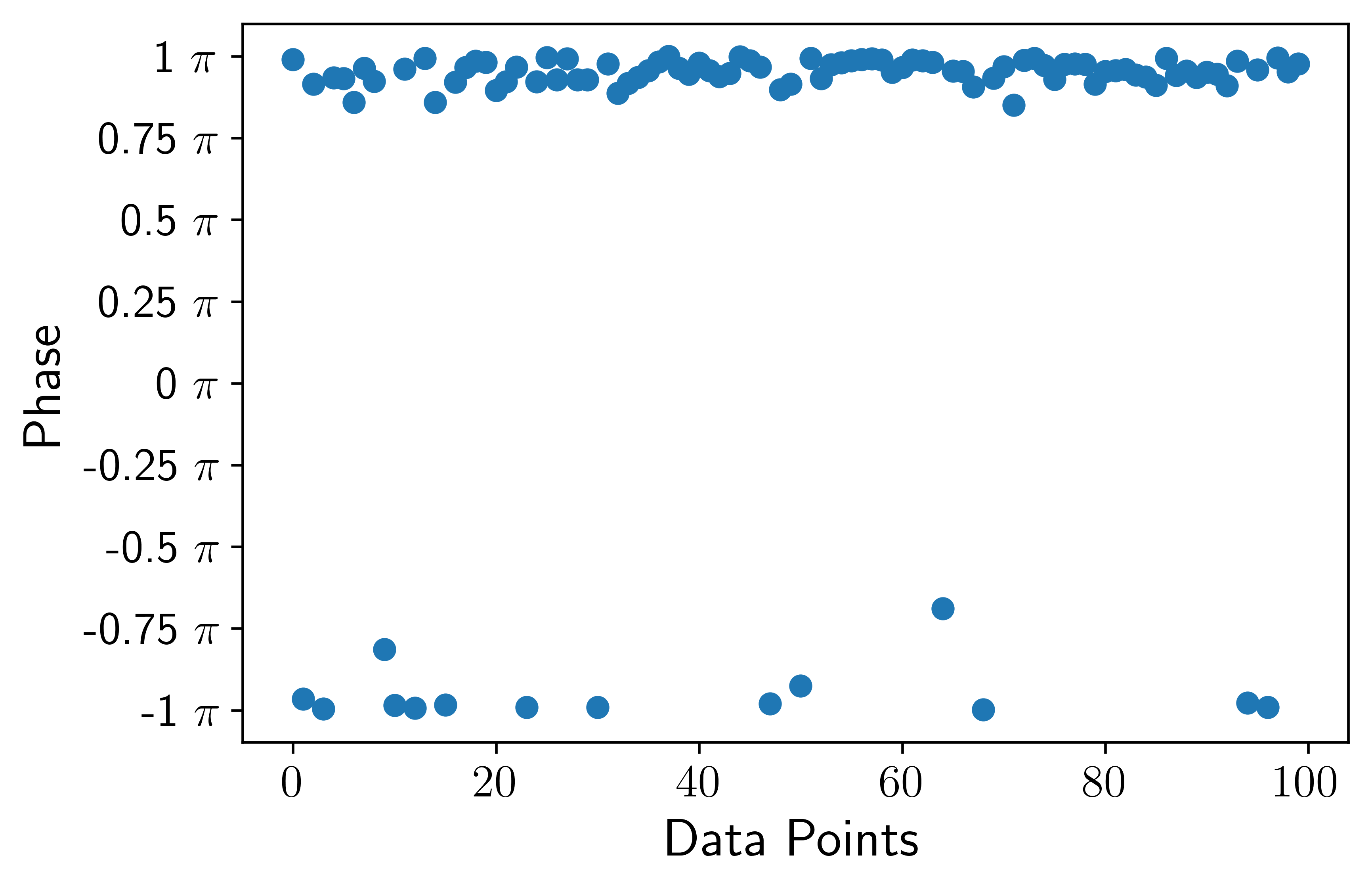
Figure 5: Phase discontinuity. Phase difference can produce an artificial discontinuity.

Input: ${\bf s}^{\textnormal{all}}=\{s_{i}\}_{i=1}^{n_{s}}$

Output: ${\bf{s}}^{k},~{}{\cal I}_{\beta^{\ast}}$

Select ${\bf s}^{0}$;

Train a DNN to obtain ${\cal I}_{\beta^{\ast}}$ using ${\bf s}^{0}$;

while $1<=k<=n_{s-1}$ do

        $i^{\ast}\mathrel{\mathop{\mathchar 58\relax}}=\arg\min_{i}R^{2}({\bf s}^{k-1},s_{i})$;

        if $R^{2}({\bf s}^{k-1},{s}_{i^{\ast}})<r_{a}$ then

               ${\bf s}^{k}={\bf s}^{k-1}\cup{s}_{i^{\ast}}$;

               Train a DNN to obtain ${\cal I}_{\beta^{\ast}}$ using ${\bf s}^{k}$;

              

       else

               exit;

              

        end if

       $k=k+1$;

end while

Algorithm 1 Selection of measurement acquisition system.

6 Implementation

We solve our forward problem employing a semi-analytic method [23, 24]. The method is implemented in an in-house Fortran 90 code [19]. Using the earth model $E_{5}$ and $45$ different measurements, we produce a large dataset (ground truth) of $300,000$ samples. Computations take almost two days to produce such dataset using a personal computer.

We use Tensorflow 2.0 [32, 30] and Keras [33] libraries to build our DNN model architecture for training. We employ the two-step loss function described in Equations 6 and 7. First, we train a DNN to produce the forward approximate ${\cal F}_{\alpha^{\ast}}$ following Equation 6, and then use the trained DNN and Equation 7 to produce the approximate inverse operator ${\cal I}_{\beta^{\ast}}$. We employ a simpler DNN architecture to approximate ${\cal F}$ than the one to approximate ${\cal I}$ since the forward function $\cal F$ is well-posed and continuous, while the inverse operator $\cal{I}$ is not even well-defined. The full architecture is described in [1]. We use an NVIDIA Quadro GV100 GPU for training.

To reduce the computational cost of Algorithm 1, we first execute it using $30,000$ samples. Once we obtain our final measurement acquisition system, we train our DNN with the entire dataset. The algorithm needs seven iterations with this reduced dataset and almost $44$ hours of processing time to obtain the final measurement acquisition system. In the last iteration, we spend $53$ hours for training using the entire dataset composed of $300,000$ samples. The details of processing time is given in Table 5. We can afford these $96$ hours, i.e., $4$ days of processing time for entire simulation as it is offline. Once we obtain the trained DNN, we need a fraction of a second to evaluate the inverse solution.

problem	data size	iterations	epochs	processing time [$\mathrm{h}$]
Forward and inverse	$30,000$	$7$	$1200$	$43.77$
Forward	$300,000$	$1$	$1200$	$18.69$
Inverse	$300,000$	$1$	$3000$	$34.41$

Table 5: Training times of the DNN.

7 Numerical Results

In this section, we describe our iterative algorithm for designing the measurement acquisition system. At each iteration, we evaluate the performance of the DNN-based inversion with an updated measurement acquisition system. For evaluation of the DNN approximation, different varieties of cross-plots of DNN-predicted measurement against ground truth provide us with important information [1]. We focus here on two types of cross-plots that are crucial for the assessment of DNN-based inversions:

Cross-plots 1:	$\mathcal{F}\circ\mathcal{I}$	vs	$\mathcal{F}\circ\mathcal{I}_{\beta^{\ast}}$
Cross-plots 2:	$\mathcal{I}$	vs	$\mathcal{I}_{\beta^{\ast}}$

Cross-plots of type 1 depict how well the composition of predicted inverse operator and forward function approximates the original measurements $\mathbf{m}$. These cross-plots indicate the quality of the inverse approximation. When the correlation is high, we can state that the DNN training has been successful. On the other side, cross-plots of type 2 also reflect on the non-uniqueness of $\cal I$. It is possible to obtain low-correlated cross-plots of type 2 due to non-uniqueness of $\cal I$ while cross-plots 1 exhibit high correlation.

7.1 Optimization of measurement acquisition system

We start our training with the coaxial measurement with short-spaced LWD instrument because they provide a fair assessment of the resistivity of the formation near the well. This measurement is essential to characterize $\rho_{h}$, which is a basic quantity needed to obtain a good inversion result.

Iteration 1.

In this iteration, we obtain the first approximation of ${\cal I}_{\beta^{\ast}}$ using a measurement acquisition system with the coaxial measurement with the short-spaced LWD instrument. After that, we calculate the $R^{2}$ factor of all other measurements. The algorithm selects the worst correlated measurement, which corresponds to the symmetrized directional measurement with the short-spaced deep azimuthal instrument, as depicted in Figure 6. We only display attenuation in the figures for brevity. However, the algorithm considers $R^{2}$ values of both phase difference and attenuation except for those measurements where phase differences show an artificial discontinuity.

This selection is consistent with the known physics of borehole resistivity logging instruments since the symmetrized directional measurement in a horizontal well can differentiate between the top and bottom, while co-axial measurements are unable to make such a distinction. Thus, a directional measurements is needed to distinguish between the upper and lower layers.

We observe the predicted values for subsurface material properties for each iteration in the corresponding row of Figures 10 and 11. We select three properties $\rho_{h},~{}\rho_{u},~{}d_{u}$ for illustration. The poor correlation in the first iteration hints at the inadequacy of a single measurement acquisition system.

Iteration 2.

In this iteration, the dataset with the worst correlated measurement from the previous iteration, i.e., the symmetrized directional measurement with short-spaced deep azimuthal instrument, is selected. After training, the algorithm finds that the worst correlated measurement corresponds to the symmetrized directional measurement with short-spaced LWD instrument.

Iteration $1$

0ptCoaxial measurement with the short-spaced LWD instrument

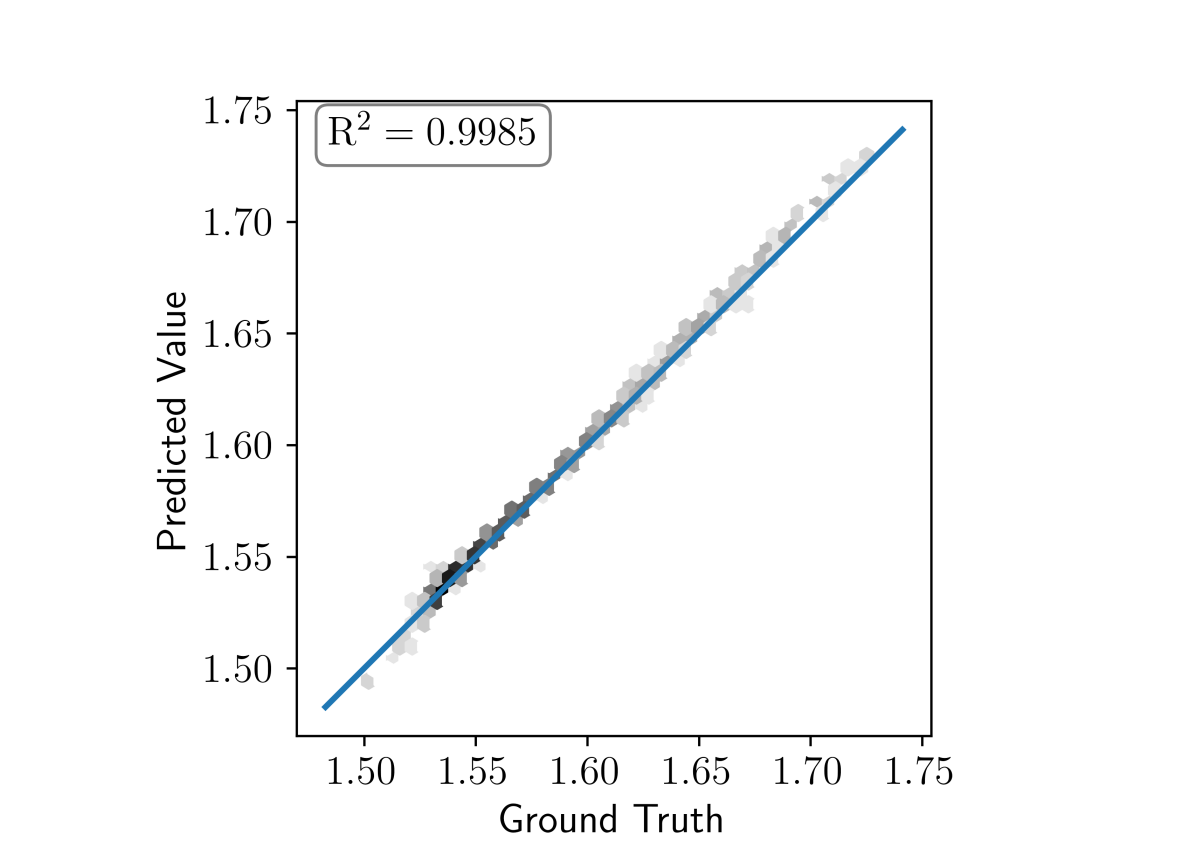
(a) *

0ptSymmterized directional measurement with the short-spaced deep azimuthal instrument

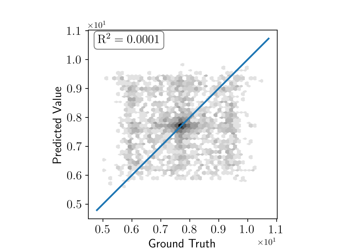
(b) *

Iteration $2$

0ptSymmterized directional measurement with the short-spaced deep azimuthal instrument

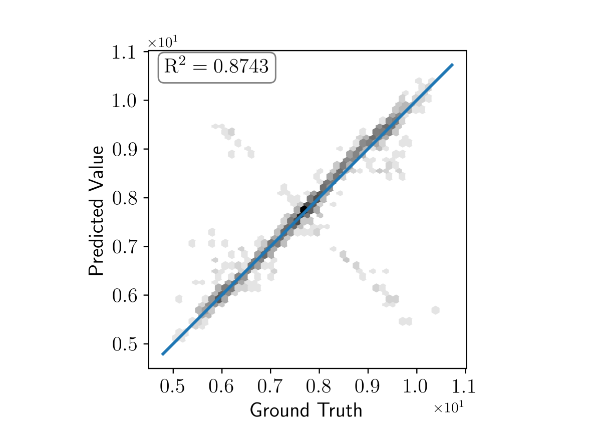
(c) *

0ptSymmetrized directional measurement with the short-spaced LWD instrument

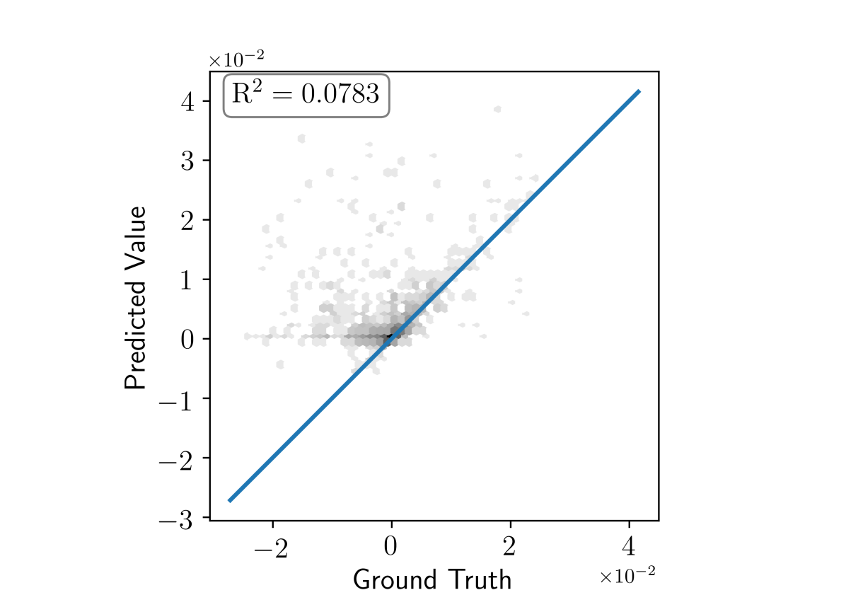
(d) *

Figure 6: Cross-plots of type 1. Predicted value vs. ground truth for attenuation – iterations $12$. First column corresponds to the last added measurement and second column is associated with the measurement with the worst $R^{2}$ value (after averaging the $R^{2}$ values of attenuation and phase).

Iteration 3.

The algorithm selects the symmetrized directional measurement with the short-spaced LWD instrument and train the DNN in this iteration. Using this trained DNN, the worst correlated measurement corresponds to the geosignal measurement with the short-spaced LWD instrument.

Iteration 4.

In this iteration, the algorithm adds the geosignal measurement with the short-spaced LWD instrument and trains the DNN. Using this trained DNN, the worst correlated measurement corresponds to the coaxial measurement with the long-spaced deep azimuthal instrument.

Iteration $3$

0ptSymmetrized directional measurement with the short-spaced LWD instrument

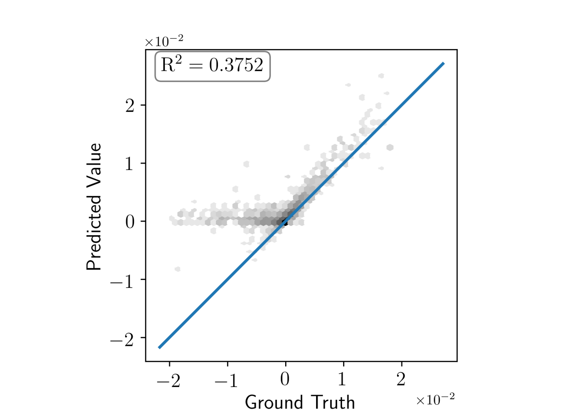
(a) *

0ptGeosignal measurement with the short-spaced LWD instrument

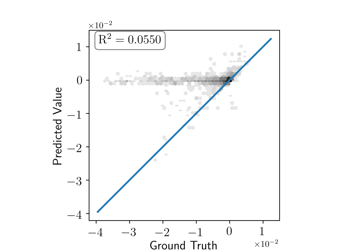
(b) *

Iteration $4$

0ptGeosignal measurement with the short-spaced LWD instrument

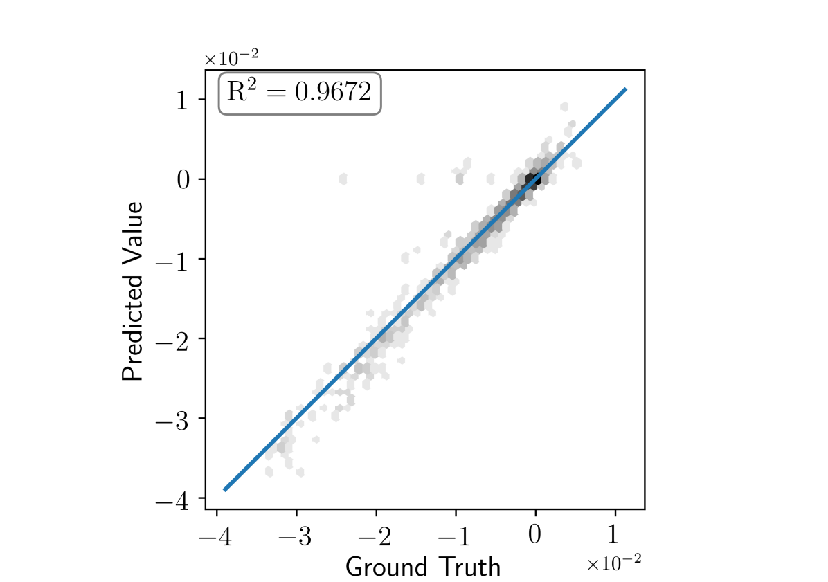
(c) *

0ptCoaxial measurement with the long-spaced deep azimuthal instrument

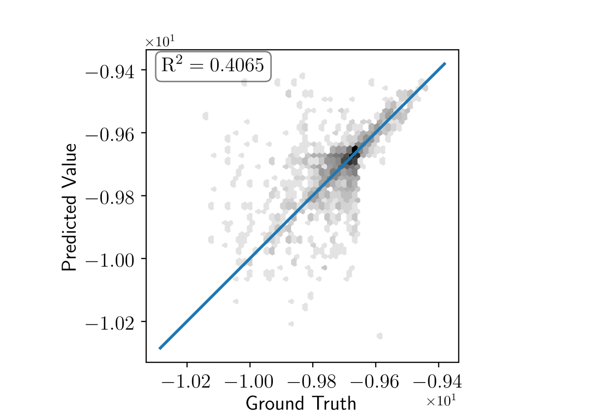
(d) *

Figure 7: Cross-plots of type 1. Predicted value vs. ground truth for attenuation–iterations $34$. First column corresponds to the last added measurement and second column is associated with the measurement with the worst $R^{2}$ value (after averaging the $R^{2}$ values of attenuation and phase).

Iteration 5.

The algorithm selects the coaxial measurement with the long-spaced deep azimuthal instrument for further training the DNN. We find that the worst averaged correlation corresponds to the symmetrized directional measurement with the long-spaced LWD instrunent.

Iteration 6.

In this iteration, the dataset with the symmetrized directional measurement using the long-spaced LWD instrument is added for further training. Using this trained DNN, we find that the worst averaged correlation corresponds to the yy-measurement using the short-spaced LWD instrument. Although the $R^{2}$ value for attenuation is high for the yy-measurement using the short-spaced LWD instrument (right panel of the third row of Figure 8), low $R^{2}$ value of phase difference makes this measurement the worst correlated one.

Iteration $5$

0ptCoaxial measurement with the long-spaced deep azimuthal instrument

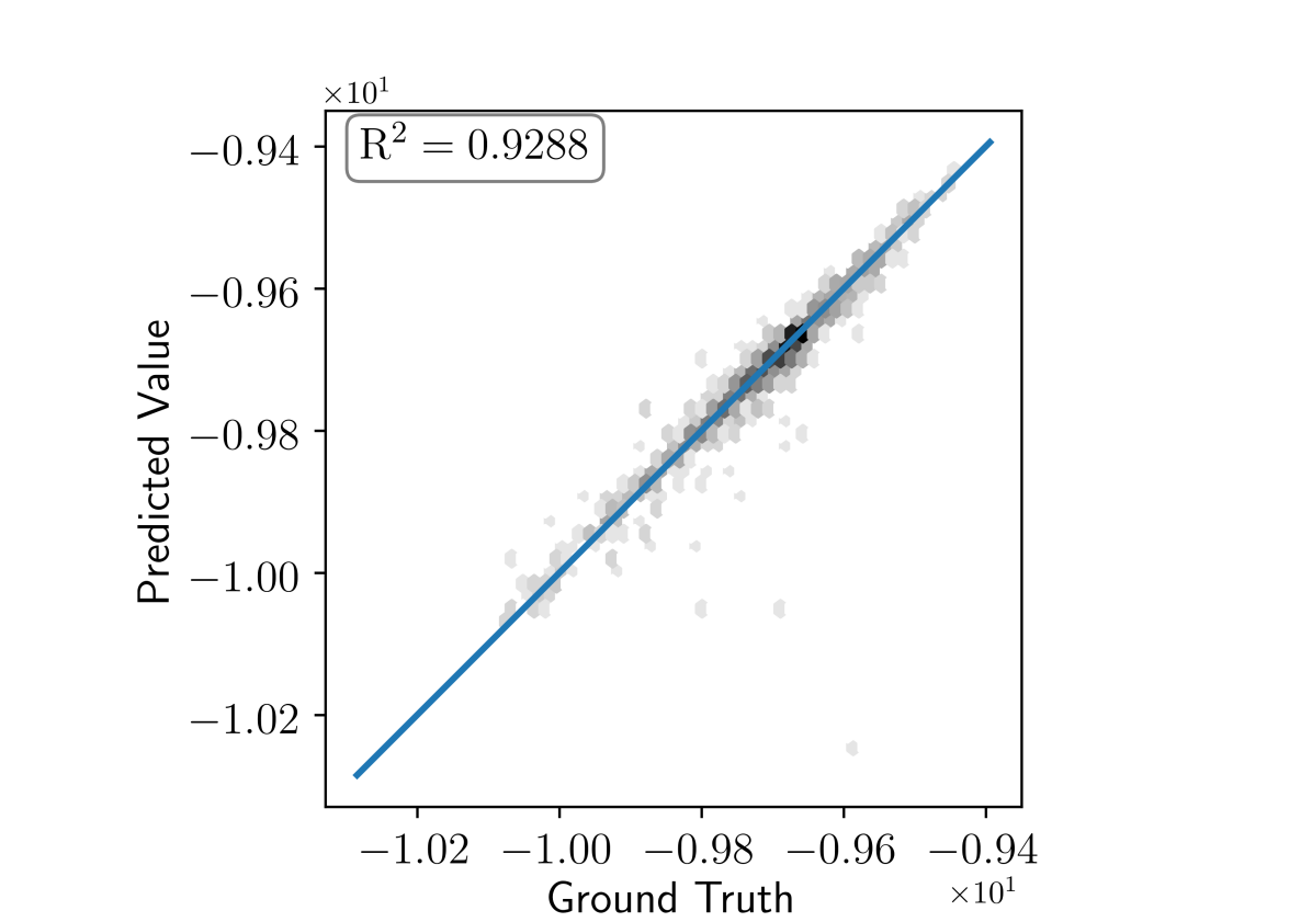
(a) *

0ptSymmterized directional measurement with the long-spaced LWD instrument

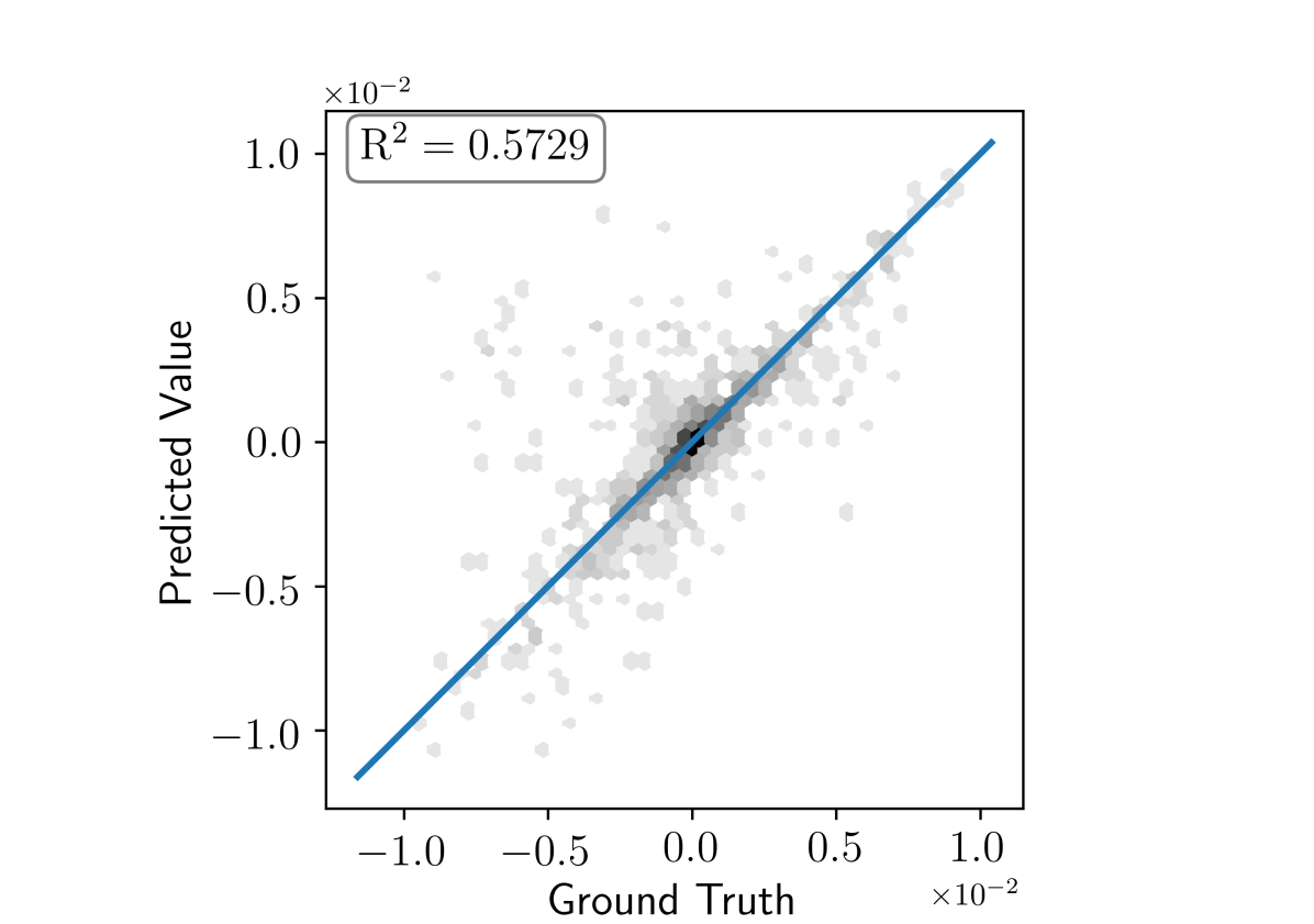
(b) *

Iteration $6$

0ptSymmterized directional measurement with the long-spaced LWD instrument

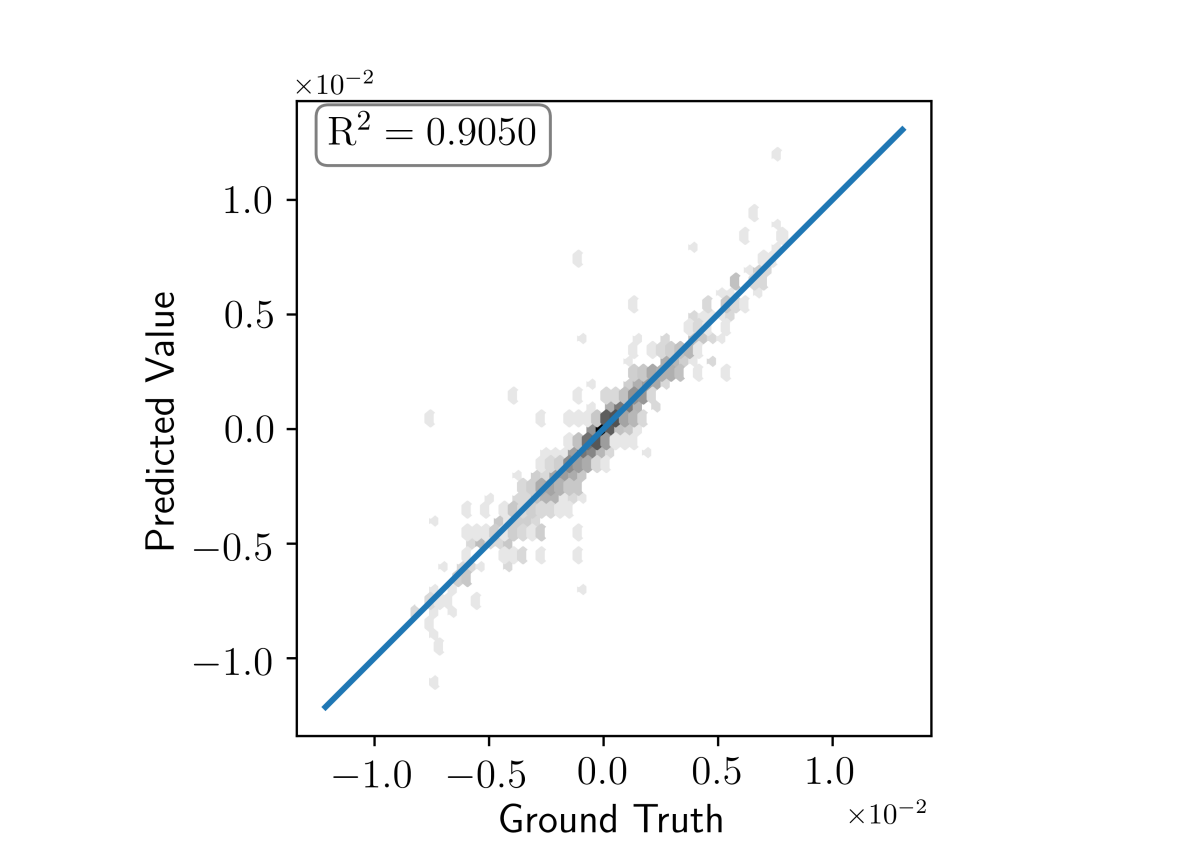
(c) *

0ptyy-measurement with the short-spaced LWD instrument

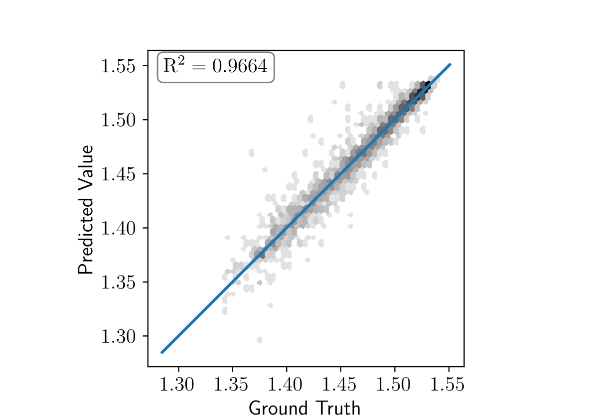
(d) *

Figure 8: Cross-plots of type 1. Predicted value vs. ground truth for attenuation–iterations $56$. First column corresponds to the last added measurement and second column is associated with the measurement with the worst $R^{2}$ value (after averaging the $R^{2}$ values of attenuation and phase).

Iteration 7.

In this iteration, the yy-measurement with the short-spaced LWD instrument is added for further training. Using this trained DNN, we find that the worst averaged correlation corresponds to the xxyyzz-measurement using the short-spaced deep azimuthal instrument. The correlation improves over the previous iteration and the average $R^{2}$ value of the worst correlation is above $0.8$. At this point, we stop adding measurements and fix our final measurement acquisition system.

Iteration 8.

In this iteration, we retrain our DNN using our last upgraded acquisition system with the entire dataset, and we observe that the average $R^{2}$ value of the worst correlation is above $0.9$.

Iteration $7$

0ptyy-measurement with the short-spaced LWD instrument

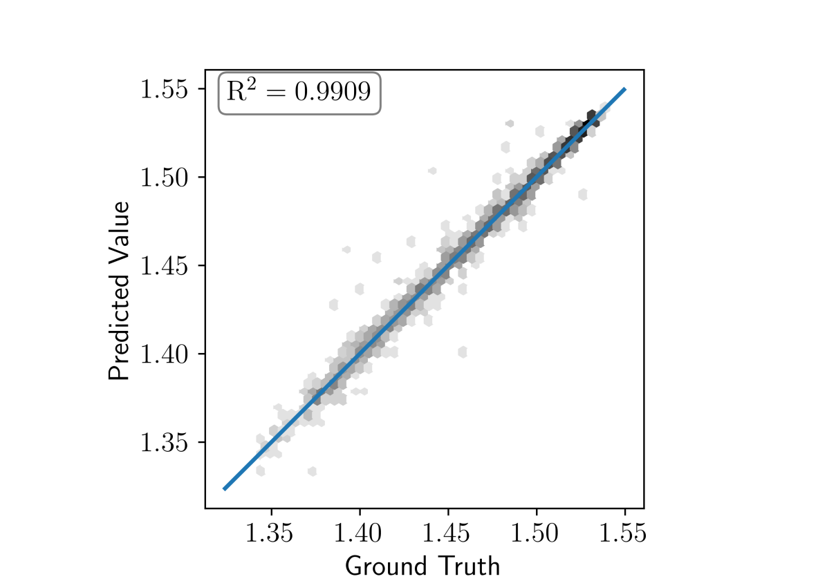
(a) *

0ptxxyyzz-measurement with the short-spaced deep azimuthal instrument

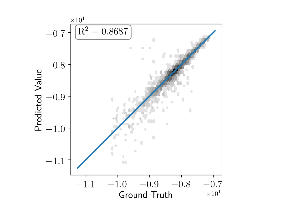
(b) *

Final Iteration

0ptyy-measurement with the short-spaced LWD instrument

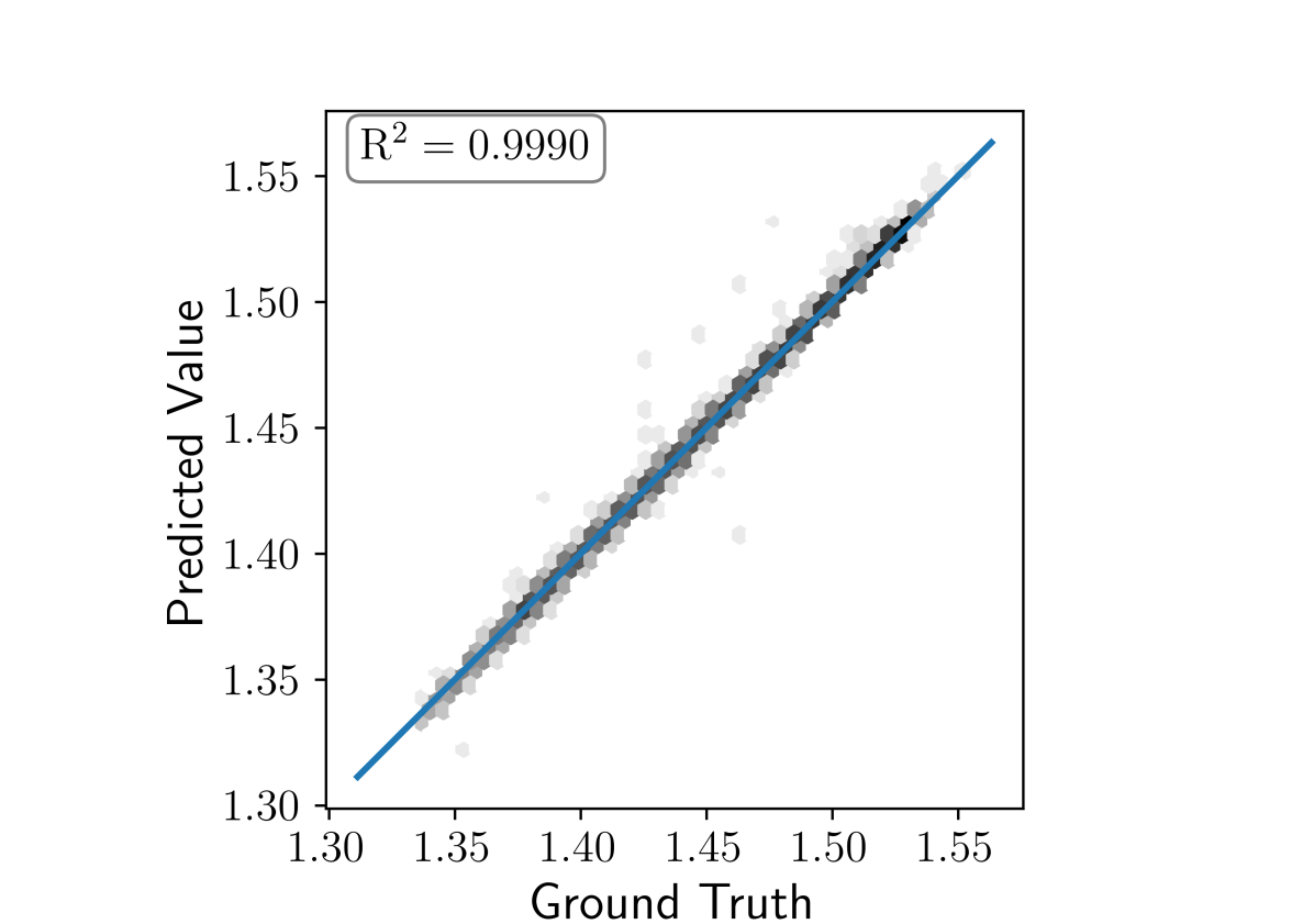
(c) *

0ptxxyyzz-measurement with the short-spaced deep azimuthal instrument

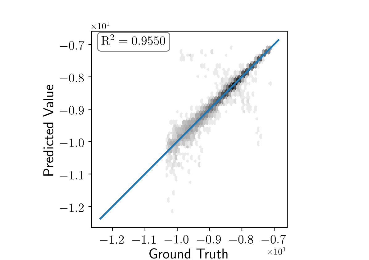
(d) *

Figure 9: Cross-plots of type 1. Predicted value vs. ground truth of attenuation for iteration $7$ and the final. First column corresponds to the last added measurement and second column is associated with the measurement with the worst $R^{2}$ value (after averaging the $R^{2}$ values of attenuation and phase).

Figures 10 and 11 compare the ground truth vs. predicted values of the inversion variables and show the improvements of predictions over different iterations. The bottom row in Figure 11 shows the final comparison between estimated and real values of subsurface properties. We observe from different rows in Figures 10 and 11 that although the resistivity predictions improve rapidly, the distance prediction $d_{u}$ takes a larger number of iterations to reach a high correlation with the ground truth. This is consistent with the physics of the problem: it is more challenging to determine bed boundary locations than resistivities.

Iteration $1$

$\rho_{h}$

$\rho_{u}$

$d_{u}$

Iteration $2$

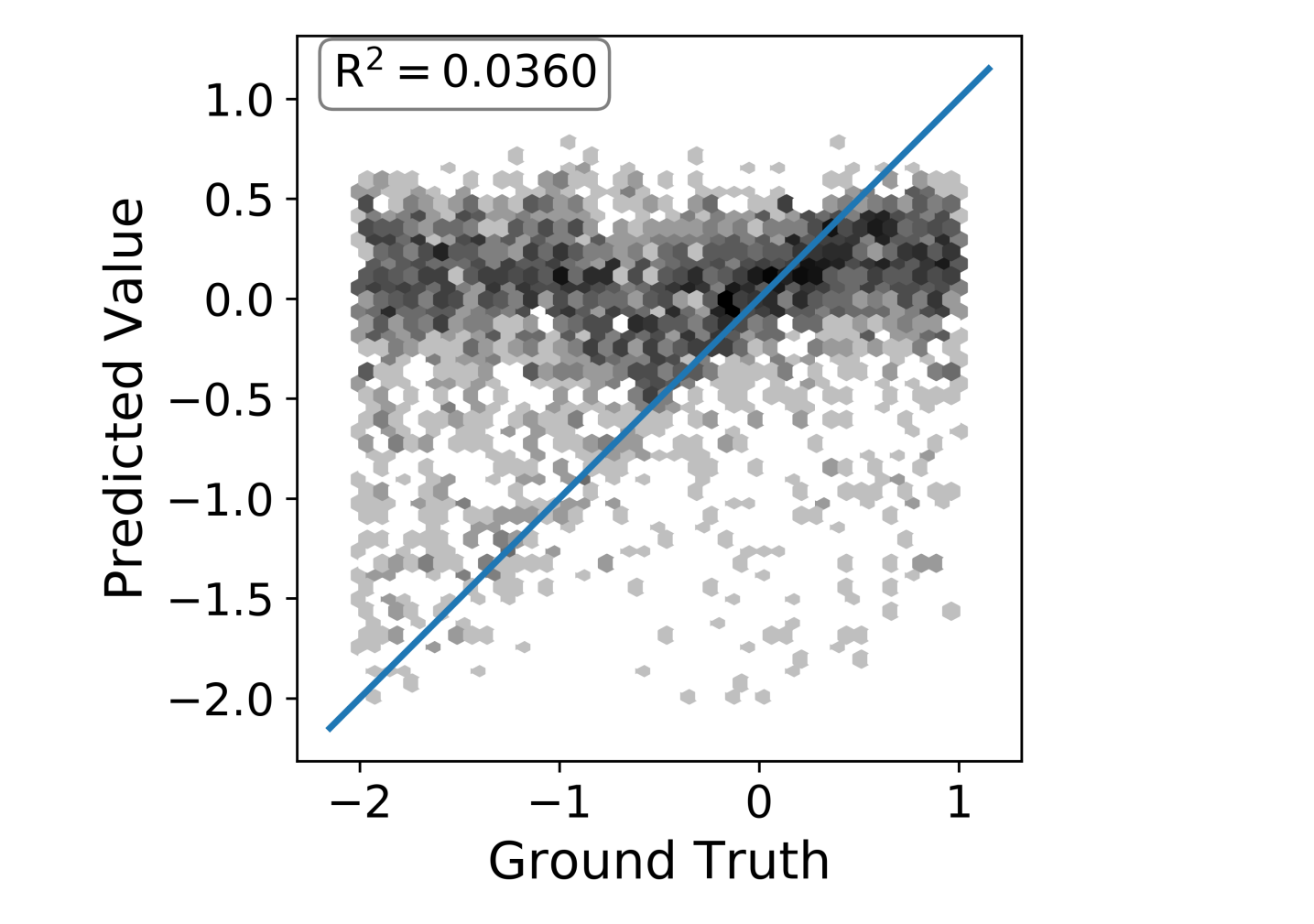
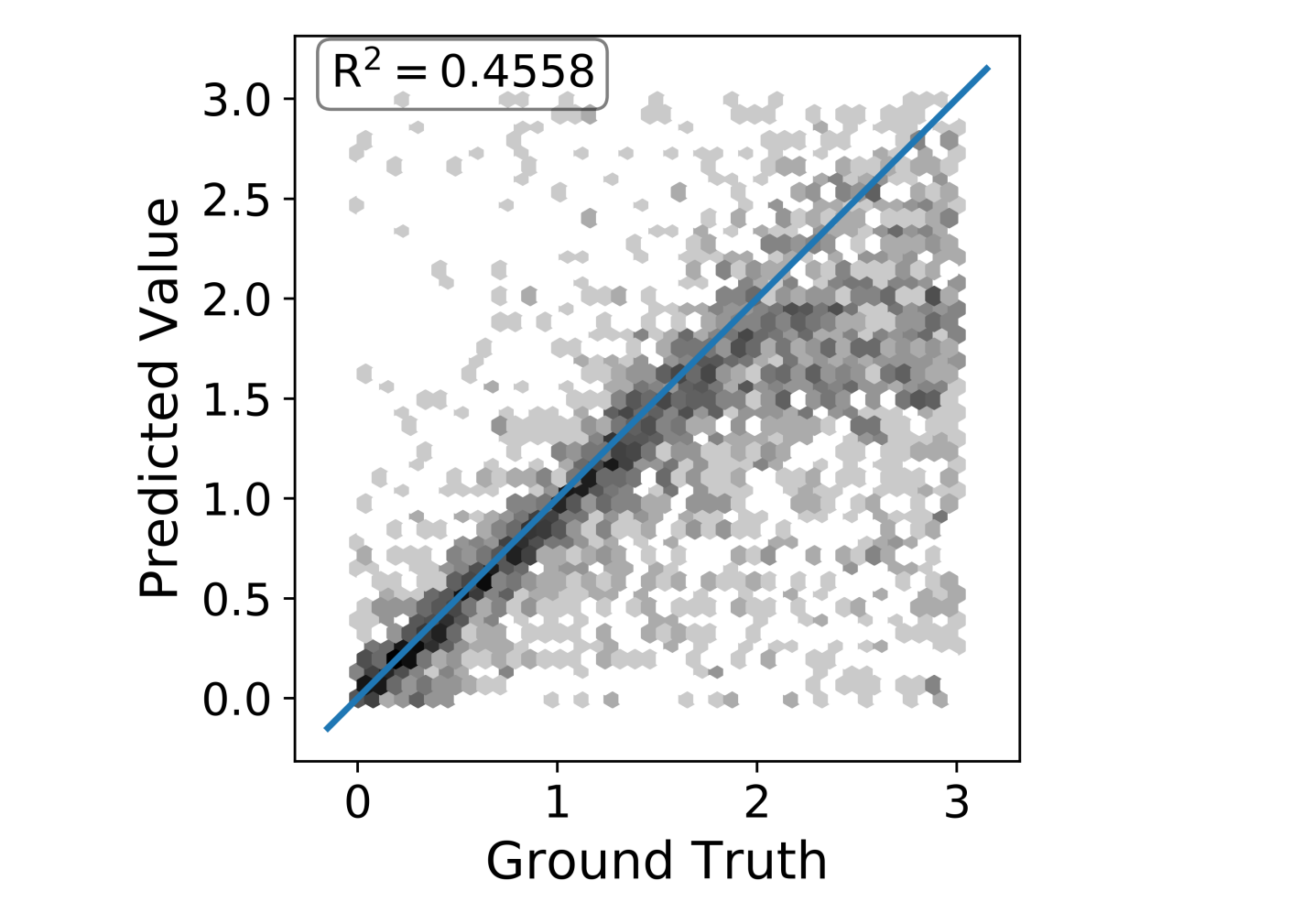
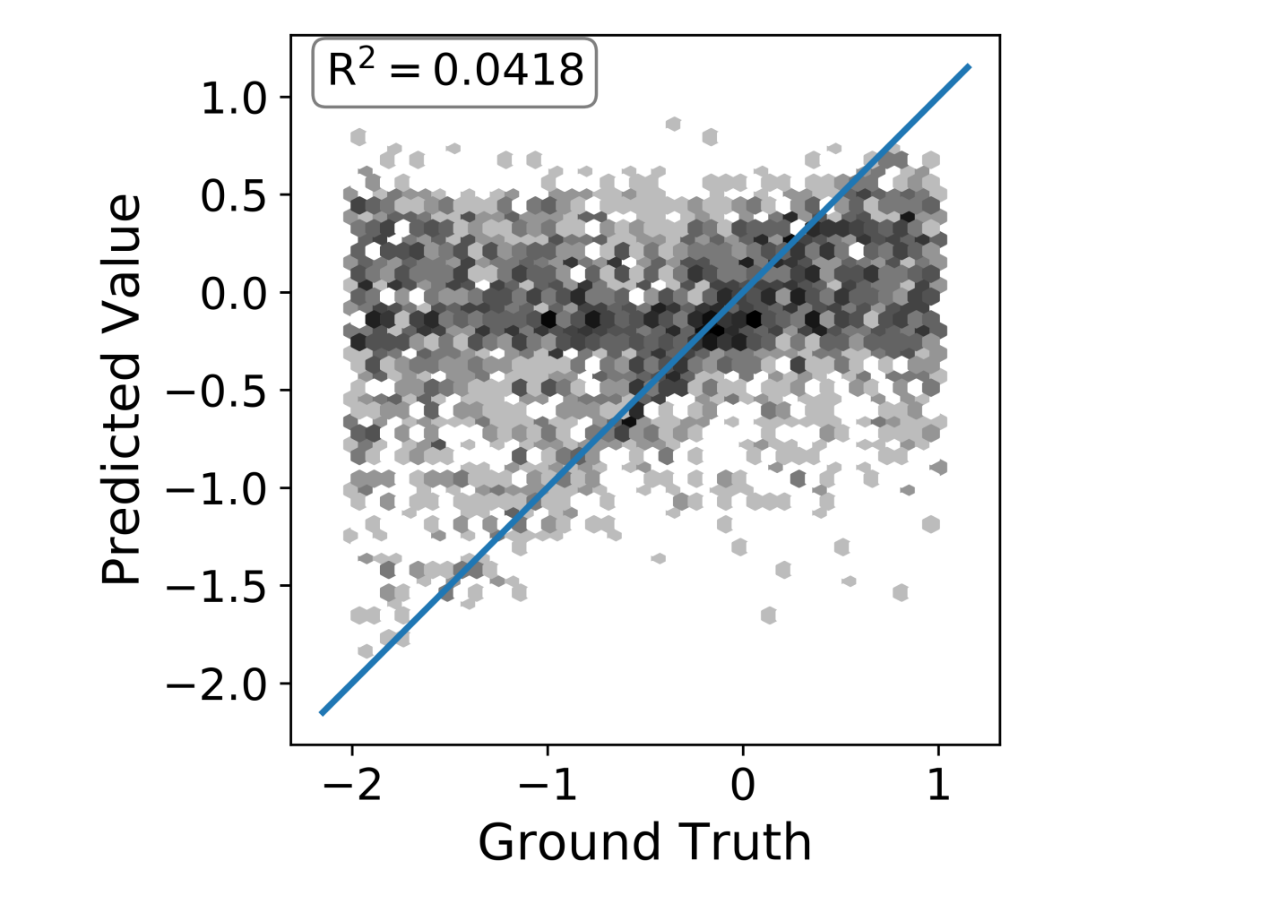
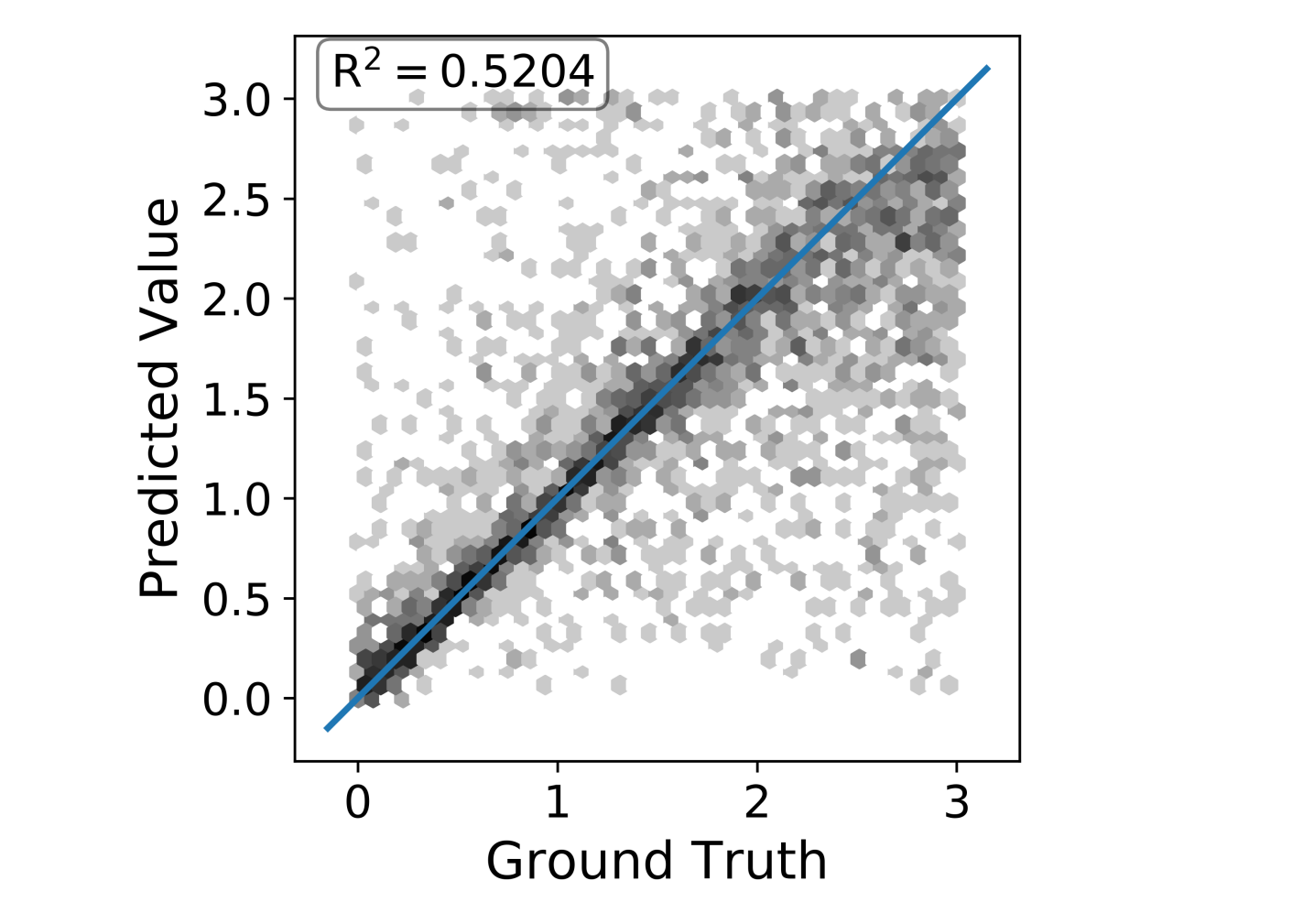
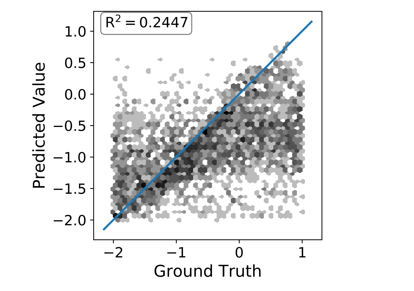
Figure 10: Predicted value vs ground truth for three subsurface material properties. Horizontal resistivity $\rho_{h}$, resistivity of layer located above the current layer $\rho_{u}$, and vertical distance from the current logging position to the upper boundary $d_{u}$ .

Iteration $3$

      Iteration $4$

Iteration $5$

$\rho_{h}$

$\rho_{u}$

$d_{u}$

Iteration $6$

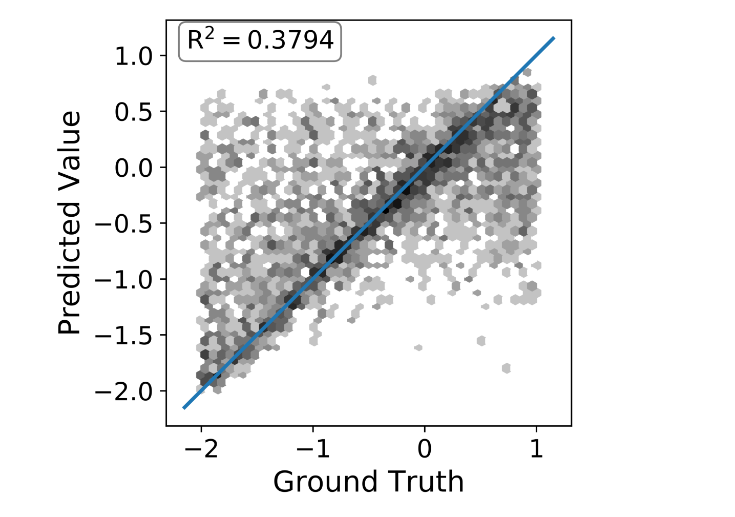
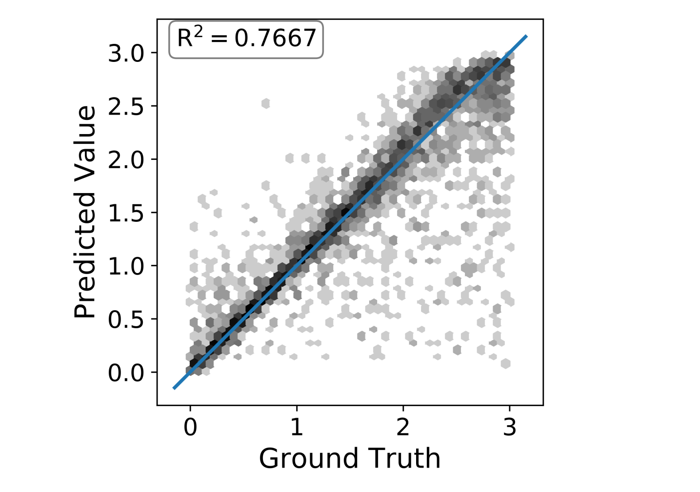
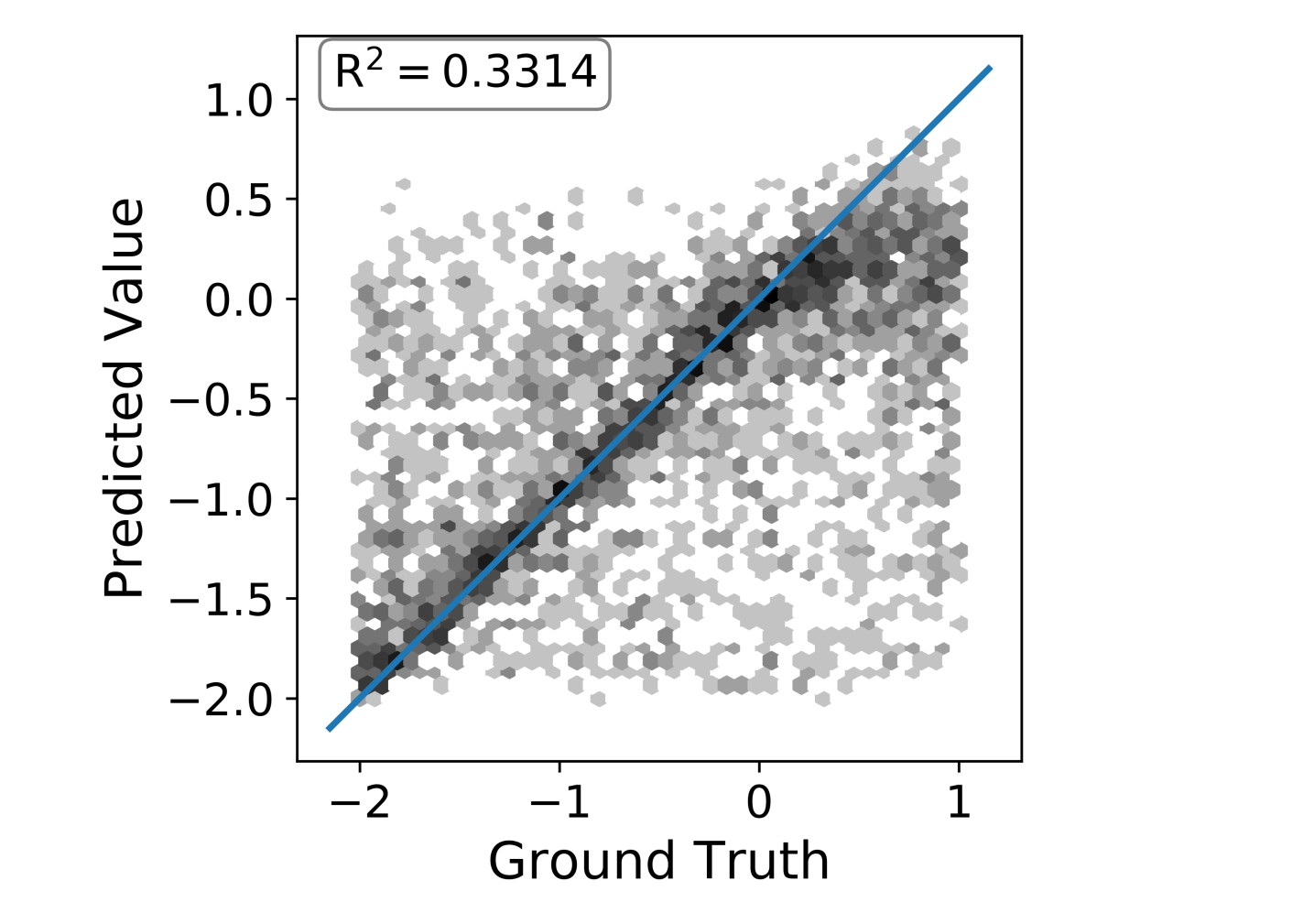
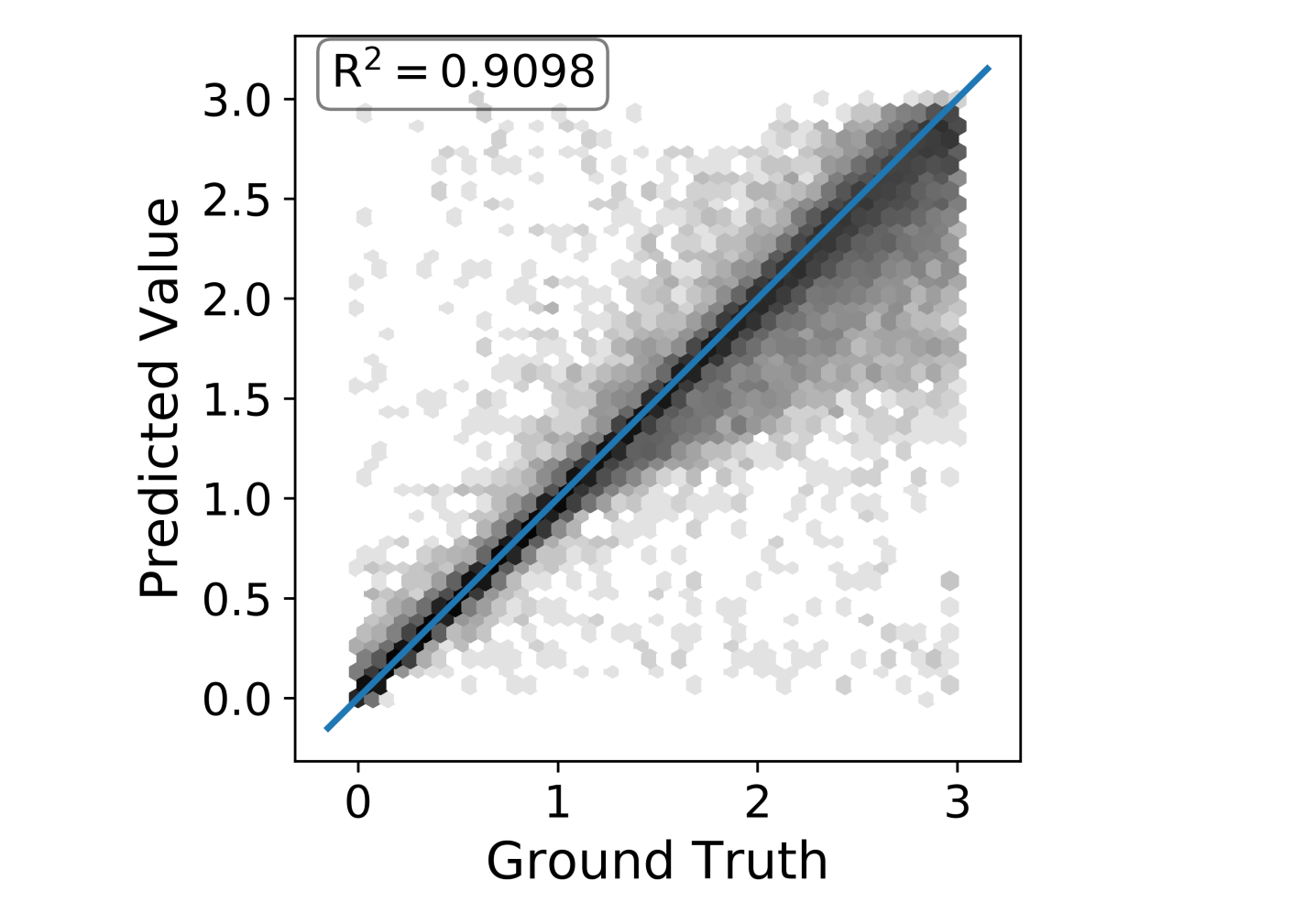
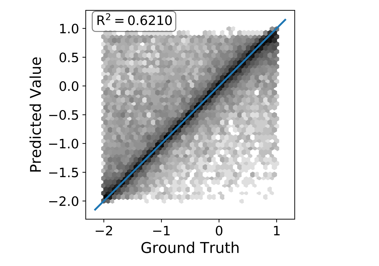
Figure 11: Predicted value vs ground truth for three subsurface material properties: horizontal resistivity $\rho_{h}$, resistivity of layer located above the current layer $\rho_{u}$, and vertical distance from the current logging position to the upper boundary $d_{u}$ for different iterations.

Iteration $7$
      Final Iteration

7.2 Inversion of realistic synthetic model

We assess the performance of the inversion process with two realistic synthetic test cases:

Model problem 1.

We create a model with realistic geological features as depicted on the top panel of Figure 12. The model has a resistive layer with a water-saturated layer underneath in the bottom left and right and it exhibits two geological faults. The trajectory dip angle varies from $82\mathrm{°}$ to $96\mathrm{°}$.

In subsequent rows of Figure 12, we observe the improvements in predictions with different iterations. We conclude that the final prediction with the final upgraded measurement acquisition system and larger dataset can properly predict the formation resisitivity at a distance of up to $57\text{\,}\mathrm{m}$ from the logging instrument.

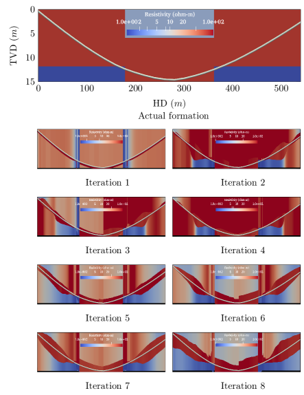
Figure 12: Model problem 1. The evolution of the inverted formation at each iteration compared to the actual formation. The gray line indicates the well trajectory.

Model problem 2.

We consider a geological formation with a conductive layer surrounded by two different resistive layers on top and bottom. The top panel of Figure 13 displays the original model. The trajectory dip angle varies from $82\mathrm{°}$ to $96\mathrm{°}$.

We conclude that the final prediction with the final upgraded measurement acquisition system can predict the targeted resistive layer from a few meters distance.

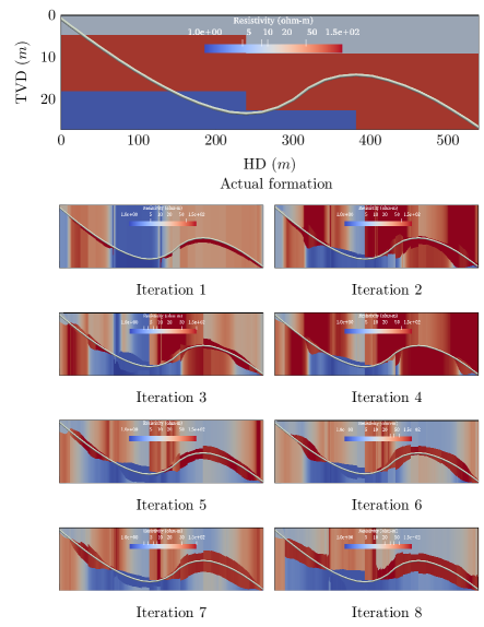
Figure 13: Model problem 2. The evolution of the inverted formation at each iteration compared to the actual formation. The gray line indicates the well trajectory.

8 Discussion and Conclusion

This paper focuses on the use of deep neural networks (DNNs) for the inversion of borehole resistivity measurements for geosteering applications. Specifically, we propose an iterative method for designing a measurement acquisition system and illustrate the effectiveness of the method with several benchmark examples.

Prior work [1] shows that a loss function based on data misfit is unsuitable for inversion due to the non-uniqueness of the inverse problem. As a remedy to that, it is possible to use a loss function specifically designed for encoder-decoder architectures with regularization. However, regularization terms hide some of the possibly existing solutions of the inverse problem. Here, we avoid regularization and employ a two-step loss function.

We then design a measurement acquisition system. We start with a single measurement and iteratively select a minimal set of measurements from a large set. By analyzing the inversion of borehole resistivity measurements, we encounter that seven carefully selected measurements is enough to uniquely determine the earth subsurface with the selected parameterization. Numerical results show that the resulting measurement acquisition system is sufficient to identify both resistive and conductive layers above and below the logging instrument. It also allows to anticipate the presence of a water-bearing layer a few vertical meters in advance, as well as to provide a proper distance estimation from that layer to the logging instrument.

Future work includes: (a) to consider noisy measurements (b) to use more general earth subsurface parameterizations (c) to consider statistics other than $R^{2}$ [34] for driving the algorithm that selects an optimal measurement acquisition system (d) to use transfer learning for inversion of 2D and 3D geometries (e) to automate different tasks in the ML pipeline using AutoML [35, 36] techniques for data processing, DNN architecture optimization, feature selection and hyperparameter tuning.

References

- [1] M. Shahriari et al. “Error Control and Loss Functions for the Deep Learning Inversion of Borehole Resistivity Measurements” doi: https://doi.org/10.1002/nme.6593 In International Journal for Numerical Methods in Engineering, 2020 DOI: https://doi.org/10.1002/nme.6593
- [2] Anatja Samouëlian et al. “Electrical resistivity survey in soil science: a review” In Soil and Tillage research 83.2 Elsevier, 2005, pp. 173–193
- [3] BR Spies “Electrical and electromagnetic borehole measurements: A review” In Surveys in Geophysics 17.4 Springer, 1996, pp. 517–556
- [4] S.. Bakr, D. Pardo and T. Mannseth “Domain decomposition Fourier FE method for the simulation of 3D marine CSEM measurements” In J. Comput. Phys. 255, 2013, pp. 456–470
- [5] S. Constable and L.. Srnka “An introduction to marine controlled-source electromagnetic methods for hydrocarbon exploration” In Geophysics 72 (2), 2007, pp. WA3–WA12
- [6] Rita Streich “Controlled-source electromagnetic approaches for hydrocarbon exploration and monitoring on land” In Surveys in geophysics 37.1 Springer, 2016, pp. 47–80
- [7] K. Key “1D inversion of multicomponent, multifrequency marine CSEM data: Methodology and synthetic studies for resolving thin resistive layers” In Geophysics 74 (2), 2009, pp. F9–F20
- [8] K. Key “Is the fast Hankel transform faster than quadrature?” In Computer Physics Communications 77 (3), 2012, pp. F21–F30
- [9] J. Alvarez-Aramberri and D. Pardo “Dimensionally adaptive hp-finite element simulation and inversion of 2D magnetotelluric measurements” In Journal of Computational Science 18, 2017, pp. 95–105
- [10] S. Davydycheva and T. Wang “A fast modelling method to solve Maxwell’s equations in 1D layered biaxial anisotropic medium” In Geophysics 76 (5), 2011, pp. F293–F302
- [11] O. Ijasana, C. Torres-Verdín and W.. Preeg “Inversion-based petrophysical interpretation of logging-while-drilling nuclear and resistivity measurements” In Geophysics 78 (6), 2013, pp. D473–D489
- [12] Sergey Alyaev et al. “A decision support system for multi-target geosteering” In Journal of Petroleum Science and Engineering 183, 2019, pp. 106381 DOI: https://doi.org/10.1016/j.petrol.2019.106381
- [13] A. Tarantola “Inverse Problem Theory and Methods for Model Parameter Estimation” Society for IndustrialApplied Mathematics, 2005
- [14] V. Puzyrev “Deep learning electromagnetic inversion with convolutional neural networks” In Geophysical Journal International 218.2, 2019, pp. 817–832
- [15] C. Vogel “Computational Methods for Inverse Problems” Society for IndustrialApplied Mathematics, 2002
- [16] D. Watzenig “Bayesian inference for inverse problems- statistical inversion” In Elektrotechnik & Informationstechnik 124, 2007, pp. 240–247
- [17] Mostafa Shahriari et al. “A deep learning approach to the inversion of borehole resistivity measurements” In Computational Geosciences 24 Springer, 2020, pp. 971–994
- [18] Aymeric-Pierre Peyret, Joaquı́n Ambía, Carlos Torres-Verdín and Joachim Strobel “Automatic Interpretation of Well Logs with Lithology-Specific Deep-Learning Methods” In SPWLA 60th Annual Logging Symposium, 2019 Society of PetrophysicistsWell-Log Analysts
- [19] M. Shahriari et al. “A numerical 1.5D method for the rapid simulation of geophysical resistivity measurements” In Geosciences 8(6), 2018, pp. 1–28
- [20] Marcela S Novo, Luiz C Da Silva and Fernando L Teixeira “Three-dimensional finite-volume analysis of directional resistivity logging sensors” In IEEE transactions on geoscience and remote sensing 48.3 IEEE, 2009, pp. 1151–1158
- [21] S. Davydycheva, D. Homan and G. Minerbo “Triaxial induction tool with electrode sleeve: FD modeling in 3D geometries” In Journal of Applied Geophysics 67, 2004, pp. 98–108
- [22] Hwa Ok Lee, Fernando L Teixeira, Luis E San Martin and Michael S Bittar “Numerical modeling of eccentered LWD borehole sensors in dipping and fully anisotropic Earth formations” In IEEE Transactions on Geoscience and Remote Sensing 50.3 IEEE, 2011, pp. 727–735
- [23] L.. Loseth and B. Ursin “Electromagnetic fields in planarly layered anisotropic media” In Geophysical Journal International 170, 2007, pp. 44–80
- [24] D. Pardo and C. Torres-Verdín “Fast 1D inversion of logging-while-drilling resistivity measurements for the improved estimation of formation resistivity in high-angle and horizontal wells” In Geophysics 80 (2), 2014, pp. E111–E124
- [25] Jay L Devore “Probability and Statistics for Engineering and the Sciences” Cengage learning, 2011
- [26] D. Moghadas “One-dimensional deep learning inversion of electromagnetic induction data using convolutional neural network” In Geophysical Journal International 222.1, 2020, pp. 247–259
- [27] Ian Goodfellow, Yoshua Bengio, Aaron Courville and Yoshua Bengio “Deep learning” MIT press Cambridge, 2016
- [28] C.. Higham and D.. Higham “Deep learning: An introduction for applied mathematicians” In Computing Research Repository abs/1801.05894, 2018
- [29] Yuchen Jin, Xuqing Wu, Jiefu Chen and Yueqin Huang “Using a Physics-Driven Deep Neural Network to Solve Inverse Problems for LWD Azimuthal Resistivity Measurements” In SPWLA 60th Annual Logging Symposium, 2019 Society of PetrophysicistsWell-Log Analysts
- [30] Martín Abadi et al. “TensorFlow: A System for Large-Scale Machine Learning” In Proceedings of the 12th USENIX Conference on Operating Systems Design and Implementation, OSDI’16 Savannah, GA, USA: USENIX Association, 2016, pp. 265–283
- [31] V. Badrinarayanan, A. Kendall and R. Cipolla “SegNet: A Deep Convolutional Encoder-Decoder Architecture for Image Segmentation” In IEEE Transactions on Pattern Analysis and Machine Intelligence 39.12, 2017, pp. 2481–2495
- [32] Martı́n Abadi et al. “TensorFlow: Large-Scale Machine Learning on Heterogeneous Systems” Software available from tensorflow.org, 2015
- [33] François Chollet “Keras” In GitHub repository GitHub, https://github.com/fchollet/keras, 2015
- [34] Tarald O Kvålseth “Cautionary note about ” In The American Statistician 39.4 Taylor & Francis, 1985, pp. 279–285
- [35] Xin He, Kaiyong Zhao and Xiaowen Chu “AutoML: A survey of the state-of-the-art” In Knowledge-Based Systems 212, 2021, pp. 106622 DOI: https://doi.org/10.1016/j.knosys.2020.106622
- [36] Frank Hutter, Lars Kotthoff and Joaquin Vanschoren “Automated machine learning: methods, systems, challenges” Springer Nature, 2019