Lattice ground states for embedded-atom models in 2D and 3D

Abstract.

The Embedded-Atom Model (EAM) provides a phenomenological description of atomic arrangements in metallic systems. It consists of a configurational energy depending on atomic positions and featuring the interplay of two-body atomic interactions and nonlocal effects due to the corresponding electronic clouds. The purpose of this paper is to mathematically investigate the minimization of the EAM energy among lattices in two and three dimensions. We present a suite of analytical and numerical results under different reference choices for the underlying interaction potentials. In particular, Gaussian, inverse-power, and Lennard-Jones-type interactions are addressed.

1. Introduction

Understanding the structure of matter is a central scientific and technological quest, cutting across disciplines and motivating an ever increasing computational effort. First-principles calculations deliver accurate predictions but are often impeded by the inherent quantum complexity, as systems size up [30]. One is hence led to consider a range of approximations. The minimization of empirical atomic pair-potentials represents the simplest of such approximations being able to describe specific properties of large-scaled atomic systems. Still, atomic pair-interactions fall short of describing the basic nature of metallic bonding, which is multi-body by nature, and often deliver inaccurate predictions of metallic systems.

The Embedded-Atom Model (EAM) is a semi-empirical, many-atom potential aiming at describing the atomic structure of metallic systems by including a nonlocal electronic correction. Introduced by Daw and Baskes [17], it has been used to address efficiently different aspects inherent to atomic arrangements including defects, dislocations, fracture, grain boundary structure and energy, surface structure, and epitaxial growth. Proving capable of reproducing experimental observations and being relatively simple to implement, the Embedded-Atom Model is now routinely used in molecular dynamic simulations [19, 28]. In particular, it has been applied in a variety of metallic systems [22], including alkali metals Li, Na, K [20, 27, 38], transition metals Fe, Ni, Cu, Pd, Ag, Pt, Au [14, 23, 27, 28], post-transition metals Al, Pb [14, 25, 35], the metalloid Si [4], and some of their alloys [14, 26].

In the case of a metallic system with a single atomic species, the EAM energy is specified as

$$\sum_{i}F(\overline{\rho}_{i})+\sum_{i\not=j}\phi(|x_{i}-x_{j}|)\quad\text{with}\quad\overline{\rho}_{i}=\sum_{j\not=i}\rho(|x_{i}-x_{j}|).$$

Here, $\{x_{i}\}$ indicate atomic positions in ${\mathbb{R}}^{d}$ and the long-range interaction potential $\phi\colon\mathbb{R}_{+}:=(0,\infty)\to\mathbb{R}_{+}$ modulates atomic pair-interactions. Atomic positions induce electronic-cloud distributions. The function $\rho\colon\mathbb{R}_{+}\to\mathbb{R}_{+}$ models the long-range electron-cloud contribution of an atom placed at $x_{j}$ on an atom placed at $x_{i}$. The sum $\overline{\rho}_{i}$ describes the cumulative effect on the atom placed at $x_{i}$ of the electronic clouds related to all other atoms. Eventually, the function $F\colon\mathbb{R}_{+}\to\mathbb{R}_{+}$ describes the energy needed to place (embed) an atom at position $x_{i}$ in the host electron gas created by the other atoms at positions $\{x_{j}\}$.

Purely pair-interaction potentials can be re-obtained from the EAM model by choosing $F=0$ and have been the subject of intense mathematical research under different choices for $\phi$. The reader is referred to [13] for a survey on the available mathematical results. The setting $F=0$ corresponds indeed to the so-called Born-Oppenheimer approximation [30], which is well adapted to the case of very low temperatures and is based on the subsequent solution of the electronic and the atomic problem. As mentioned, this approximation turns out to be not always appropriate for metallic systems at finite temperatures [35, 8] and one is asked to tame the quantum nature of the problem. This is however very challenging from the mathematical viewpoint and rigorous optimality results for point configurations in the quantum setting are scarce [12, 11]. The EAM model represents hence an intermediate model between zero-temperature phenomenological pair-interaction energies and quantum systems. Electronic effects are still determined by atomic positions, but in a more realistic nonlocal fashion when $F$ is nonlinear, resulting in truly multi-body interaction systems, see [17, 21, 35] and [19] for a review.

The aim of this paper is to investigate point configurations minimizing the EAM energy. Being interested in periodic arrangements, we restrict our analysis to the class of lattices, namely infinite configurations of the form $L=\oplus_{i=1}^{d}\mathbb{Z}u_{i}$ where $\{u_{i}\}_{i=1}^{d}$ is a basis of $\mathbb{R}^{d}$. This reduces the optimality problem to finite dimensions, making it analytically and numerically amenable. In particular, the EAM energy-per-atom of the lattice $L$ takes the specific form

$$\mathcal{E}[L]=F\Big{(}\sum_{q\in L\setminus\{0\}}\rho(|q|)\Big{)}+\sum_{q\in L\setminus\{0\}}\phi(|q|).$$

In the classical pair-interaction case $F=0$, the lattice energy $\mathcal{E}$ has already received attention and a variety of results are available, see [29, 32, 15, 5, 10, 9] and the references therein. Such results are of course dependent on the choice of the potential $\phi$. Three reference choices for $\phi$ are the Gaussian $\phi(r)=e^{-\pi\delta r^{2}}$ for $\delta>0$, the inverse-power law $\phi(r)=r^{-s}$ for $s>d$, and the Lennard-Jones-type form $\phi(r)=ar^{-\alpha}-br^{-\beta}$ for $d<\beta<\alpha$ and $a,\,b>0$. In the Gaussian case, it has been shown by Montgomery [29] that, for all $\delta>0$, the triangular lattice of unit density is the unique minimizer (up to isometries) of $\mathcal{E}$ with $F=0$ among unit-density lattices. The same can be checked for the the inverse-power-law case by a Mellin-transform argument. More generally, the minimality of the triangular lattice of unit density is conjectured by Cohn and Kumar in [15, Conjecture 9.4] to hold among all unit-density periodic configurations. This fact is called universal optimality and has been recently proved in dimension $8$ and $24$ for the lattice $\mathsf{E}_{8}$ and the Leech lattice $\Lambda_{24}$, respectively [16]. In the Lennard-Jones case, the minimality in 2d of the triangular lattice at fixed density has been investigated in [11, 5], the minimality in 3d of the cubic lattice is proved in [7], and more general properties in arbitrary dimensions have been investigated in [10]. A recap of the main properties of the Lennard-Jones case is presented in Subsection 2.3. These play a relevant role in our analysis.

In this paper, we focus on the general case $F\not=0$, when $F$ is nonlinear. More precisely, we discuss the reference cases of embedding functions $F$ of the form

$$F(r)=r^{t}\log(\gamma r)\quad\text{or}\quad F(r)=r^{t}$$

for $t,\,\gamma>0$. The first, logarithmic choice is the classical one chosen to fit with the so-called Universal Binding Curve (see e.g., [31]) and favoring a specific minimizing value $r_{0}>0$, see [2, 14]. The second, power-law form favors on the contrary $r_{0}=0$ and allows for a particularly effective computational approach. Let us mention that other choices for $F$ could be of interest. In particular, the form $F(r)=-c\sqrt{r}$, $c>0$, is related to the Finnis-Sinclair model [21] and is discussed in Remark 4.3. Some of our theory holds for general functions $F$, provided that they are minimized at a sole value $r_{0}$. We call such functions of one-well type.

The electronic-cloud contribution function $\rho\colon\mathbb{R}_{+}\to\mathbb{R}_{+}$ is assumed to be decreasing and integrable. We specifically focus on the Gaussian and inverse-power law

$$\rho(r)=e^{-\delta r^{2}}\quad\text{or}\quad\rho(r)=r^{-s}$$

for $\delta>0$ and $s>d$, discussed, e.g., in [39] and [17, 21, 35], respectively.

As for the pair-interaction potential $\phi\colon\mathbb{R}_{+}\to\mathbb{R}_{+}$, we assume a Lennard-Jones-type form [3, 34] or an inverse-power law [17, 35], i.e.,

$$\phi(r)=ar^{-\alpha}-br^{-\beta}\quad\text{or}\quad\phi(r)=r^{-\alpha}$$

for $d<\beta<\alpha$ and $a,\,b>0$. Note that short-ranged potentials $\phi$ have been considered as well [17, 18].

Our main theoretical results amount at identifying minimizers in the specific reference case of $F(r)=r\log r$ and $\rho(r)=r^{-s}$. More precisely, we find the following:

• (Inverse-power law) If $\phi(r)=r^{-\alpha}$, the minimizers of $\mathcal{E}$ coincide with those of the Lennard-Jones potential $r\mapsto r^{-\alpha}-r^{-s}$, up to rescaling (Theorem 4.1);
  

• (Lennard-Jones) If $\phi(r)=ar^{-\alpha}-br^{-\beta}$, under some compatibility assumptions on the parameters, the minimizers of $\mathcal{E}$ coincide with those of the Lennard-Jones potential $r\mapsto r^{-\alpha}-r^{-s}$ (Theorem 5.2).

Actually, both results hold for more general embedding functions $F$, see (4.1) and Remarks 4.2–4.5. With this at hand, the problem can be reduced to the pure Lennard-Jones case (i.e., $F=0$) which is already well understood. In particular, in the two dimensional case we find that the triangular lattice, up to rescaling and isometries, is the unique minimizer of $\mathcal{E}$ in specific parameters regimes. These theoretical findings are illustrated by numerical experiments in two and three dimensions. By alternatively choosing the Gaussian $\rho(r)=e^{-\delta r^{2}}$, in two dimensions we additionally observe the onset of a phase transition between the triangular and an orthorhombic lattice, as $\delta$ decreases. In three dimensions, both in the inverse-power-law case $\rho(r)=r^{-s}$ and in the Gaussian case $\rho(r)=e^{-\delta r^{2}}$, the simple cubic lattice $\mathbb{Z}^{3}$ is favored against the face-centered and the body-centered cubic lattice for $s$ or $\delta$ small, respectively.

In the power-law case $F(r)=r^{t}$, for $\rho$ of inverse-power-law type and $\phi$ of Lennard-Jones type and specific, physically relevant choices of parameters, one can conveniently reduce the complexity of the optimization problem from the analytical standpoint. This reduction allows to explicitly compute the EAM energy for any lattice of unit density, hence allowing to investigate numerically minimality in two and three dimensions. Depending on the parameters, the relative minimality of the triangular, square, and orthorhombic lattices in two dimensions and the simple cubic, body-centered cubic, and face-centered cubic lattices in three dimension is ascertained.

This is the plan of the paper: Notation on potentials and energies are introduced in Subsections 2.1 and 2.2. The two subcases $F=0$ and $\phi=0$ are discussed in Subsection 2.3 and in Section 3, respectively. In particular, known results on Lennard-Jones-type interactions are recalled in Subsection 2.3. The inverse-power-law case $\phi(r)=r^{-\alpha}$ is investigated in Section 4. The Lennard-Jones case $\phi(r)=ar^{-\alpha}-br^{-\beta}$ is addressed theoretically and numerically in Section 5. In particular, Subsection 5.1 contains the classical case $F(r)=r\log r$, and Subsection 5.2 discusses the power-law case $F(r)=r^{t}$.

2. Notation and preliminaries

2.1. Lattices

For any dimension $d$, we write $\mathcal{L}_{d}$ for the set of all lattices $L=\bigoplus_{i=1}^{d}\mathbb{Z}u_{i}$, where $\{u_{i}\}_{i=1}^{d}$ is a basis of $\mathbb{R}^{d}$. We write $\mathcal{L}_{d}(1)\subset\mathcal{L}_{d}$ for the set of all lattices with unit density, which corresponds to $|\det(u_{1},\ldots,u_{d})|=1$.

In dimension two, any lattice $L\in\mathcal{L}_{2}(1)$ can be written as

$$L:=\mathbb{Z}\left(\frac{1}{\sqrt{y}},0\right)\oplus\mathbb{Z}\left(\frac{x}{\sqrt{y}},\sqrt{y}\right),$$

for $(x,y)\in\mathcal{D}$, where

$$\mathcal{D}=\big{\{}(x,y)\in\mathbb{R}^{2}\,:\,0\leq x\leq 1/2,\,y>0;\,x^{2}+y^{2}\geq 1\big{\}}$$ (2.1)

is the so-called (half) fundamental domain for $\mathcal{L}_{2}(1)$ (see, e.g., [29, Page 76]). In particular, the square lattice $\mathbb{Z}^{2}$ and the triangular lattice with unit density, denoted by $\mathsf{A}_{2}\in\mathcal{L}_{d}(1)$, are given by the respective choices $(x,y)=(0,1)$ and $(x,y)=\left(1/2,{\sqrt{3}}/{2}\right)$, i.e.,

$$\mathbb{Z}^{2}=\mathbb{Z}(1,0)\oplus\mathbb{Z}(0,1)\quad\text{ and }\quad\mathsf{A}_{2}:=\sqrt{\frac{2}{\sqrt{3}}}\left[\mathbb{Z}(1,0)\oplus\mathbb{Z}\left(\frac{1}{2},\frac{\sqrt{3}}{2}\right)\right].$$

In dimension three, the fundamental domain of $\mathcal{L}_{3}(1)$ is much more difficult to describe (see e.g., [36, Section 1.4.3]) and its 5-dimensional nature makes it impossible to plot compared to the 2-dimensional $\mathcal{D}$ defined in (2.1). The Face-Centered Cubic (FCC) and Body-Centered Cubic (BCC) lattices with unit density are respectively indicated by $\mathsf{D}_{3}\in\mathcal{L}_{3}(1)$ and $\mathsf{D}_{3}^{*}\in\mathcal{L}_{3}(1)$, and are defined as

$$\mathsf{D}_{3}:=2^{-\frac{1}{3}}\left[\mathbb{Z}(1,0,1)\oplus\mathbb{Z}(0,1,1)\oplus\mathbb{Z}(1,1,0)\right];$$

$$\mathsf{D}_{3}^{*}:=2^{\frac{1}{3}}\left[\mathbb{Z}(1,0,0)\oplus\mathbb{Z}(0,1,0)\oplus\mathbb{Z}\left(\frac{1}{2},\frac{1}{2},\frac{1}{2}\right)\right].$$

Remark 2.1 (Periodic configurations).

All results in this paper are stated in terms of lattices, for the sake of definiteness. Let us however point out that the same statements hold in the more general setting of periodic configurations in dimensions $d\in\{8,24\}$, on the basis of the recently proved optimality results from [16]. In dimension $d=2$, universal optimality is only known among lattices, see [29]. Still, the validity of the Cohn-Kumar conjecture (see [15, Conjecture 9.4]) would allow us to consider more general periodic configurations as well.

2.2. Potentials and energies

For any dimension $d$, let $\mathcal{S}_{d}$ be the set of all functions $f\colon\mathbb{R}_{+}\to\mathbb{R}$ such that $|f(r)|={\rm O}(r^{-d-\eta})$ for some $\eta>0$ as $r\to\infty$. By $\mathcal{S}_{d}^{+}\subset\mathcal{S}_{d}$ we denote the subset of nonnegative functions. We say that a continuous function $F\colon\mathbb{R}_{+}\to\mathbb{R}$ is a one-well potential if there exists $r_{0}>0$ such that $F$ is decreasing on $(0,r_{0})$ and increasing on $(r_{0},\infty)$.

For any $\phi\in\mathcal{S}_{d}$, we define the interaction energy $E_{\phi}\colon\mathcal{L}_{d}\to\mathbb{R}$ by

$$E_{\phi}[L]:=\sum_{q\in L\backslash\{0\}}\phi(|q|).$$ (2.2)

If $\phi(r)=r^{-s}$, $s>d$, $E_{\phi}[L]$ actually corresponds to the Epstein zeta function, which is defined by

$$\zeta_{L}(s):=\sum_{q\in L\backslash\{0\}}\frac{1}{|q|^{s}}.$$ (2.3)

For any function $F\colon\mathbb{R}_{+}\to\mathbb{R}$ and for any $\rho\in\mathcal{S}_{d}^{+}$, we define the embedding energy $E_{F,\rho}\colon\mathcal{L}_{d}\to\mathbb{R}$ by

$$E_{F,\rho}[L]:=F(E_{\rho}[L])\quad\text{with}\quad E_{\rho}[L]:=\sum_{q\in L\backslash\{0\}}\rho(|q|).$$ (2.4)

Finally, for any $\phi\in\mathcal{S}_{d}$, any $\rho\in\mathcal{S}_{d}^{+}$, and any $F\colon\mathbb{R}_{+}\to\mathbb{R}$, we define the total energy $\mathcal{E}\colon\mathcal{L}_{d}\to\mathbb{R}$ by

$$\mathcal{E}[L]:=E_{F,\rho}[L]+E_{\phi}[L]=F(E_{\rho}[L])+E_{\phi}[L].$$ (2.5)

In the following, we investigate $\mathcal{E}$ under different choices of the potentials $F$, $\rho$, and $\phi$. In some parts, we will require merely abstract conditions on the potentials, such as a monotone decreasing $\rho$ or a one-well potential $F$. In other parts, we will consider more specific potentials. In particular, we will choose, for $\gamma,\delta,t,a,b>0$, $s>d$, and $\alpha>\beta>d$,

$$F(r)\in\{r^{t},r^{t}\log(\gamma r)\},\quad\rho(r)\in\{r^{-s},e^{-\delta r^{2}}\},\quad\phi(r)\in\{r^{-\alpha},ar^{-\alpha}-br^{-\beta}\}.$$

Note that the choice of $s$, $\delta$, $\alpha$, and $\beta$ implies that $\phi\in\mathcal{S}_{d}$ and $\rho\in\mathcal{S}_{d}^{+}$, so that the sums in (2.2) and (2.4) are well defined.

For any $L\in\mathcal{L}_{d}(1)$, any $\phi\in\mathcal{S}_{d}$, any $\rho\in\mathcal{S}_{d}^{+}$, and any $F\colon\mathbb{R}_{+}\to\mathbb{R}$, we define, if they uniquely exist, the following optimal scaling parameters for the energies:

$$\lambda^{\mathcal{E}}_{L}:=\mathop{\rm argmin}\nolimits_{\lambda>0}\mathcal{E}[\lambda L],\quad\lambda^{F,\rho}_{L}:=\mathop{\rm argmin}\nolimits_{\lambda>0}E_{F,\rho}[\lambda L],\quad\lambda^{\phi}_{L}:=\mathop{\rm argmin}\nolimits_{\lambda>0}E_{\phi}[\lambda L].$$ (2.6)

2.3. A recap on the Lennard-Jones-type energy

A classical problem is to study the $F=0$ case for a Lennard-Jones-type potential

$$\phi(r)=ar^{-\alpha}-br^{-\beta},\quad\alpha>\beta>d,\quad a,\,b>0.$$ (2.7)

Let us recap some known facts in this case [5, 10], which will be used later on. We start by reducing the minimization problem on all lattices to a minimization problem on lattices of unit density only. This is achieved by computing the optimal scaling parameter of the energy $\lambda^{\phi}_{L}$ , see (2.6), for each $L\in\mathcal{L}_{d}(1)$, which in turn allows to find the minimum of the energy among dilations of $L$. More precisely, in case (2.7), for all $\lambda>0$ and all lattices $L\in\mathcal{L}_{d}(1)$, one has

$$E_{\phi}[\lambda L]=a\lambda^{-\alpha}\zeta_{L}(\alpha)-b\lambda^{-\beta}\zeta_{L}(\beta),$$

where we use (2.3). (This energy was studied first in [5, Section 6.3].) Then, we find the unique minimizer

$$\lambda^{\phi}_{L}=\left(\frac{\alpha a\zeta_{L}(\alpha)}{\beta b\zeta_{L}(\beta)}\right)^{\frac{1}{\alpha-\beta}},$$ (2.8)

and therefore the energy is given by

$$\min_{\lambda>0}E_{\phi}[\lambda L]=E_{\phi}[\lambda^{\phi}_{L}L]=\frac{b^{\frac{\alpha}{\alpha-\beta}}\zeta_{L}(\beta)^{\frac{\alpha}{\alpha-\beta}}}{a^{\frac{\beta}{\alpha-\beta}}\zeta_{L}(\alpha)^{\frac{\beta}{\alpha-\beta}}}\left(\left(\frac{\beta}{\alpha}\right)^{\frac{\alpha}{\alpha-\beta}}-\left(\frac{\beta}{\alpha}\right)^{\frac{\beta}{\alpha-\beta}}\right)<0.$$

The latter inequality follows from the fact that $\alpha>\beta$. Consequently, for any lattices $L,\Lambda\in\mathcal{L}_{d}(1)$, we have that

$$E_{\phi}[\lambda_{L}^{\phi}L]\leq E_{\phi}[\lambda^{\phi}_{\Lambda}\Lambda]\iff\frac{\zeta_{L}(\alpha)^{\beta}}{\zeta_{L}(\beta)^{\alpha}}\leq\frac{\zeta_{\Lambda}(\alpha)^{\beta}}{\zeta_{\Lambda}(\beta)^{\alpha}}.$$

This means that finding the lattice with minimal energy amounts to minimizing the function

$$L\mapsto e^{*}(L):=\frac{\zeta_{L}(\alpha)^{\beta}}{\zeta_{L}(\beta)^{\alpha}}$$ (2.9)

on $\mathcal{L}_{d}(1)$. This is particularly effective in dimension two where for fixed $(\alpha,\beta)$ the minimizer can be found numerically by plotting $L\mapsto\min_{\lambda}\mathcal{E}[\lambda L]$ in the fundamental domain $\mathcal{D}$. Figure 1 shows the case $(\alpha,\beta)=(12,6)$, i.e., when $\phi$ is the classical Lennard-Jones potential. The global minimum of $E_{\phi}$ in $\mathcal{L}_{2}$ appears to be the triangular lattice $\lambda^{\phi}_{\mathsf{A}_{2}}\mathsf{A}_{2}$.

For a certain range of parameters $(\alpha,\beta)$, this observation can be rigorously ascertained. Indeed, for $d=2$, it is shown in [5, Theorem 1.2.B.] that the global minimum of $E_{\phi}$ is uniquely achieved by a triangular lattice $\lambda_{\mathsf{A}_{2}}^{\phi}\mathsf{A}_{2}$ if

$$H(\alpha)<H(\beta),\quad\textnormal{where}\quad H(t):=\frac{1}{2}\pi^{-t/2}\Gamma\left(\frac{t}{2}\right)t,$$ (2.10)

and $\Gamma$ is the classical Gamma function $\Gamma(r)=\int_{0}^{\infty}x^{r-1}e^{x}\,{\rm d}x$ for $r>0$. (In the sequel, all statements on uniqueness are intended up to isometries, without further notice.) In fact, under condition (2.10) one has that [5]

• $\mathsf{A}_{2}$ is the unique minimizer in $\mathcal{L}_{2}(1)$ of $\displaystyle L\mapsto\lambda^{\phi}_{L}=\left(\frac{\alpha a\zeta_{L}(\alpha)}{\beta b\zeta_{L}(\beta)}\right)^{\frac{1}{\alpha-\beta}}$,

• $\mathsf{A}_{2}$ is the unique minimizer in $\mathcal{L}_{2}(1)$ of $e^{*}$ defined in (2.9).

As pointed out in [5, Remark 6.18], it is necessary to choose $2<\beta<\alpha<M\approx 9.2045818$ in order to obtain these optimality results by using the method developed there. In particular, this means that the following pairs of integer exponents can be chosen: $(\alpha,\beta)\in\{(4,3);(5,3);(6,3);(5,4);(6,4)\}$. Note that the classical Lennard-Jones potential $(\alpha,\beta)=(12,6)$ is not covered by [5, Theorem 1.2.B.].

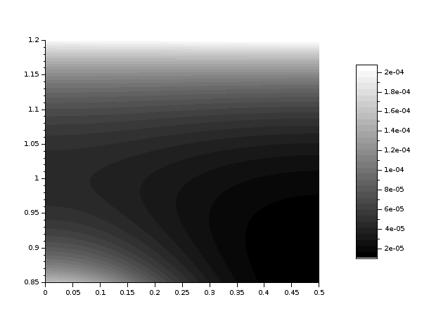
Figure 1. Contour plot of $L\mapsto e^{*}(L)=\frac{\zeta_{L}(12)^{6}}{\zeta_{L}(6)^{12}}$ in the fundamental domain $\mathcal{D}$. The triangular lattice $\mathsf{A}_{2}$ with coordinates $(1/2,\sqrt{3}/2)$ appears to be the unique minimizer. Moreover, $\mathbb{Z}^{2}$ with coordinates $(0,1)$ appears to be a saddle point.

We now ask ourselves what is the minimal scaling parameter $\lambda$ and the corresponding lattice $L\in\mathcal{L}_{d}(1)$ for which $E_{\phi}[\lambda L]$ is minimized. Physically, this would correspond to identifying the first minimum of $E_{\phi}$ starting from a high-density configuration by progressively decreasing the density. We have the following.

Proposition 2.2 (Smallest volume meeting the global minimum).

Let $\phi$ be a Lennard-Jones-type potential as in (2.7). If $L_{d}\in\mathcal{L}_{d}(1)$ is the minimizer of $L\mapsto\zeta_{L}(\beta)$ on $\mathcal{L}_{d}(1)$ and $\lambda_{L_{d}}^{\phi}L_{d}$ is the unique global minimizer of $E_{\phi}$ on $\mathcal{L}_{d}$, then $\lambda_{L_{d}}^{\phi}$ is the unique minimizer of $L\mapsto\lambda^{\phi}_{L}$ on $\mathcal{L}_{d}(1)$.

Proof.

As discussed above, if $\lambda_{L_{d}}^{\phi}L_{d}$ is a global minimizer of $E_{\phi}$ on $\mathcal{L}_{d}$, then $L_{d}$ minimizes the function $e^{*}$ defined in (2.9) on $\mathcal{L}_{d}(1)$. This yields

$$\frac{\zeta_{L_{d}}(\alpha)^{\beta}}{\zeta_{L_{d}}(\beta)^{\alpha}}\leq\frac{\zeta_{L}(\alpha)^{\beta}}{\zeta_{L}(\beta)^{\alpha}}$$ (2.11)

for all $L\in\mathcal{L}_{d}(1)$. We thus have

$$\left(\frac{\zeta_{L}(\beta)\zeta_{L_{d}}(\alpha)}{\zeta_{L}(\alpha)\zeta_{L_{d}}(\beta)}\right)^{\beta}=\frac{\zeta_{L}(\beta)^{\alpha}\zeta_{L_{d}}(\alpha)^{\beta}}{\zeta_{L}(\alpha)^{\beta}\zeta_{L_{d}}(\beta)^{\alpha}}\left(\frac{\zeta_{L_{d}}(\beta)}{\zeta_{L}(\beta)}\right)^{\alpha-\beta}\leq\left(\frac{\zeta_{L_{d}}(\beta)}{\zeta_{L}(\beta)}\right)^{\alpha-\beta}.$$

As we are assuming that $\zeta_{L_{d}}(\beta)\leq\zeta_{L}(\beta)$ for all $L\in\mathcal{L}_{d}(1)$, we further get

$$\frac{\zeta_{L}(\beta)\zeta_{L_{d}}(\alpha)}{\zeta_{L}(\alpha)\zeta_{L_{d}}(\beta)}\leq\left(\frac{\zeta_{L_{d}}(\beta)}{\zeta_{L}(\beta)}\right)^{\frac{\alpha-\beta}{\beta}}\leq 1,$$ (2.12)

where we use that $\alpha>\beta$. In view of (2.8), this shows that $\lambda^{\phi}_{L}\geq\lambda_{L_{d}}^{\phi}$ for all $L\in\mathcal{L}_{d}(1)$. If $\lambda^{\phi}_{L}=\lambda_{L_{d}}^{\phi}$, then we have a double equality in (2.12). This implies also equality in (2.11) which is equivalent to $e^{*}(L)=e^{*}(L_{d})$. Therefore, it follows that $L=L_{d}$ up to rotation, by uniqueness of the minimizer $L_{d}$ of $e^{*}$. ∎

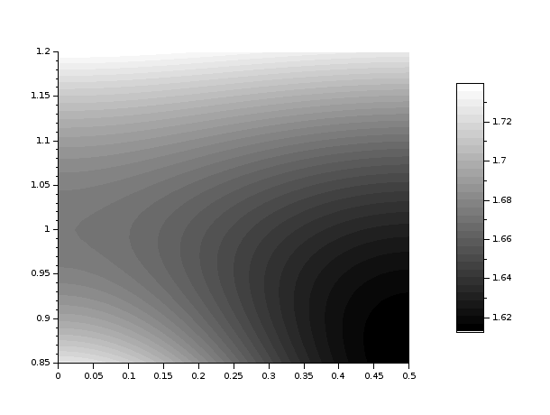
Figure 2. Contour plot of $L\mapsto(b/a)^{1/6}\lambda_{L}^{\phi}=\left(\frac{12\zeta_{L}(12)}{6\zeta_{L}(6)}\right)^{1/6}$, see (2.8), in the fundamental domain $\mathcal{D}$. The triangular lattice $\mathsf{A}_{2}$ with coordinates $(1/2,\sqrt{3}/2)$ is the unique minimizer for any choice of $a,\,b>0$.

We refer to Figure 2 for an illustration in the two-dimensional case $(\alpha,\beta)=(12,6)$. Note that in this case the global minimum is not known. Still, the triangular lattice appears to be the first stable structure reached by increasing the volume (decreasing the density). This is in agreement with Figure 1 and Proposition 2.2. Recall that the triangular lattice also minimizes $L\mapsto\zeta_{L}(\beta)$ on $\mathcal{L}_{d}(1)$, as required in the statement of Proposition 2.2, see [29].

Notice that in dimension $d=3$ there is no rigorous result concerning the minimizer of $E_{\phi}$ in $\mathcal{L}_{3}$. Only local minimality results for cubic lattices $\mathbb{Z}^{3},\mathsf{D}_{3},\mathsf{D}_{3}^{*}$ have been derived in [7]. Numerical investigations suggest that $\lambda_{\mathsf{D}_{3}}^{\phi}\mathsf{D}_{3}$ is the unique minimizer of $E_{\phi}$ in $\mathcal{L}_{3}$ for any values $\alpha>\beta>d$ of the exponents, see, e.g., [40, Figure 5], [10, Figures 5 and 6] and [7, Conjecture 1.7]. Therefore, we can conjecture that $\mathsf{D}_{3}$ is the unique minimizer of $L\mapsto\lambda_{L}^{\phi}$ in $\mathcal{L}_{3}(1)$ by application of Proposition 2.2.

3. Properties of the embedding energy $E_{F,\rho}$

In this section we focus on the properties of the embedding energy $E_{F,\rho}$ given in (2.4). Although other choices for the potential $F$ may been considered (see, e.g., [21, 19]), we concentrate ourselves on the one-well case (see, e.g., [14] and references therein). In that case, it is clear that the global minimum of $E_{F,\rho}$ in $\mathcal{L}_{d}$ can be achieved for any $L$ by simply choosing $\lambda$ such that $E_{\rho}[\lambda L]=r_{0}=\mathop{\rm argmin}\nolimits_{r>0}F(r)$. We now ask ourselves what is the minimal scaling parameter $\lambda$ and the corresponding lattice $L\in\mathcal{L}_{d}(1)$ for which $E_{F,\rho}[\lambda L]$ achieves $\min F$. In other words, what is the minimizer of $L\mapsto\lambda^{F,\rho}_{L}$ in $\mathcal{L}_{d}(1)$ (recall (2.6)). Physically, this would correspond to reach the ground state of the embedding energy $\min F$ starting from a high-density configuration by progressively decreasing the density.

Theorem 3.1 (Smallest volume meeting the global minimum).

Let $F\colon\mathbb{R}_{+}\to\mathbb{R}$ be a one-well potential and let $\rho\in\mathcal{S}^{+}_{d}$ be strictly decreasing. Then, $\lambda^{F,\rho}_{L}$ exists and $\min F$ is achieved by choosing $\lambda^{F,\rho}_{L}L$ for all $L\in\mathcal{L}_{d}(1)$. Furthermore, if $L_{d}$ is the unique minimizer in $\mathcal{L}_{d}(1)$ of $L\mapsto E_{\rho}[\lambda_{L_{d}}^{F,\rho}L]$, then $L_{d}$ is the unique minimizer in $\mathcal{L}_{d}(1)$ of $L\mapsto\lambda^{F,\rho}_{L}$.

Proof.

Let $r_{0}>0$ be the unique minimizer of $F$, namely, $F(r_{0})=\min F$. Given any $L\in\mathcal{L}_{d}(1)$, the fact that $\rho\in\mathcal{S}_{d}^{+}$ is strictly decreasing implies that $\lambda\mapsto E_{\rho}[\lambda L]$ is strictly decreasing and goes to $0$ at infinity and to $\infty$ at $0$. Therefore, there exists a unique $\lambda>0$ such that $E_{\rho}[\lambda L]=r_{0}$. Such $\lambda$ obviously coincides with $\lambda_{L}^{F,\rho}$ given in (2.6). This shows the first part of the statement.

Suppose now that $L_{d}$ is the unique minimizer in $\mathcal{L}_{d}(1)$ of $L\mapsto E_{\rho}[\lambda_{L_{d}}^{F,\rho}L]$. Assume by contradiction that there exists $L\in\mathcal{L}_{d}(1)$, $L\neq L_{d}$, with $\lambda^{F,\rho}_{L}\leq\lambda_{L_{d}}^{F,\rho}$. By using that $\lambda\mapsto E_{\rho}[\lambda L]$ is decreasing, this would imply

$$E_{\rho}[\lambda^{F,\rho}_{L}L]\geq E_{\rho}[\lambda_{L_{d}}^{F,\rho}L]>E_{\rho}[\lambda_{L_{d}}^{F,\rho}L_{d}]=r_{0}=E_{\rho}[\lambda^{F,\rho}_{L}L],$$

a contradiction. We thus deduce that $\lambda_{L_{d}}^{F,\rho}\leq\lambda^{F,\rho}_{L}$ for all $L\in\mathcal{L}_{d}(1)$, with equality if and only if $L=L_{d}$. ∎

We note that Theorem 3.1 can be applied to the choice $\rho(r)=r^{-s}$, $s>d$, and the triangular lattice $\mathsf{A}_{2}$, the $\mathsf{E}_{8}$ lattice, or the Leech lattice $\Lambda_{24}$ in dimensions $2$, $8$, and $24$, respectively. In fact, these lattices are the unique minimizer of $L\mapsto E_{\rho}[\lambda L]$ for all $\lambda>0$, see [29, 16].

Let us mention that, in this setting, asking $F$ to be one-well is not restrictive. In fact, if $F$ is a strictly increasing (resp. decreasing) function, no optimal scaling parameters $\lambda>0$ can be found since, for any $L\in\mathcal{L}_{d}(1)$, $E_{F,\rho}[\lambda L]$ will be minimized for $\lambda\to 0$ (resp. $\lambda\to\infty$).

4. The EAM energy with inverse-power interaction $\phi(r)=r^{-\alpha}$

In this section, we study the energy $\mathcal{E}$ defined in (2.5) when $\phi$ is given by the inverse-power interaction $\phi(r)=r^{-\alpha}$. The main result of this section is the following.

Theorem 4.1 (EAM energy for inverse-power interaction).

For any $\alpha>s>d$, let $\rho(r)=r^{-s}$, let $\phi(r)=r^{-\alpha}$, and let $F\in C^{1}(\mathbb{R}_{+})$. We assume that the functions

$$g(r):=r^{1-{\alpha}/{s}}F^{\prime}(r)\quad\textnormal{and}\quad h(r):=F(r)-\frac{s}{\alpha}rF^{\prime}(r)\quad\quad\text{for $r>0$}$$ (4.1)

satisfy that $g$ is strictly increasing on $I:=\{F^{\prime}<0\}$, that $g(I)=(-\infty,0)$, and that $h\circ g^{-1}$ is strictly decreasing on $(-\infty,0)$. (Note that $g^{-1}$ exists on $(-\infty,0)$ and takes values in $\mathbb{R}_{+}$.) Then, $\lambda^{\mathcal{E}}_{L}$ exists for all $L\in\mathcal{L}_{d}(1)$ and the following statements are equivalent:

• $L_{d}$ is the unique minimizer in $\mathcal{L}_{d}(1)$ of $L\mapsto e^{*}(L)=\frac{\zeta_{L}(\alpha)^{s}}{\zeta_{L}(s)^{\alpha}}$, see (2.9);

• $\lambda^{\mathcal{E}}_{L_{d}}L_{d}$ is the unique minimizer of $\mathcal{E}$ in $\mathcal{L}_{d}$;

• $\lambda_{L_{d}}^{\bar{\phi}}L_{d}$ is the unique minimizer in $\mathcal{L}_{d}$ of $E_{\bar{\phi}}$ for $\bar{\phi}(r)=r^{-\alpha}-r^{-s}$, see (2.7).

In particular, when $d=2$ and $H(\alpha)<H(s)$ where $H$ is defined by (2.10), then the unique minimizer of $\mathcal{E}$ in $\mathcal{L}_{2}$ is the triangular lattice $\lambda_{\mathsf{A}_{2}}^{\mathcal{E}}\mathsf{A}_{2}$.

Furthermore, if $L_{d}$ is the unique minimizer of $L\mapsto\zeta_{L}(s)$ in $\mathcal{L}_{d}(1)$ as well as a minimizer of $e^{*}$ in $\mathcal{L}_{d}(1)$, then $L_{d}$ is the unique minimizer of $L\mapsto\lambda^{\mathcal{E}}_{L}$ in $\mathcal{L}_{d}(1)$, where $\lambda^{\mathcal{E}}_{L}$ is defined in (2.6).

The gist of this result is the coincidence of the minimizers of $\mathcal{E}$ with those of $E_{\bar{\phi}}$ for $\bar{\phi}(r)=r^{-\alpha}-r^{-s}$ (up to proper rescaling), under quite general choices of $F$. This results in a simplification of the minimality problem for $\mathcal{E}$ as one reduces to the study of minimality for the Lennard-Jones-type potential $\bar{\phi}$, which is already well known, see Subsection 2.3. In particular, in two dimensions and under condition $H(\alpha)<H(s)$, the unique minimizer is a properly rescaled triangular lattice.

Before proving the theorem, let us present some applications to specific choices of $F$.

Remark 4.2 (Application 1 - The classical case $F(r)=r\log r$).

We can apply this theorem to $F(r)=r^{t}\log(\gamma r)$ for $t\in(0,\alpha/s)$ and $\gamma>0$ which is a one-well potential with minimum attained at point $r_{0}^{t}:=\frac{1}{\gamma}e^{-1/t}$. In particular, the case $F(r)=r\log r$ is admissible since $s<\alpha$. In fact, we have $I=(0,r_{0}^{t})$ and

$$g(r)=r^{t-\alpha/s}\big{(}t\log(\gamma r)+1),\quad g^{\prime}(r)=r^{t-\alpha/s-1}\left(\left(t-\frac{\alpha}{s}\right)(t\log(\gamma r)+1)+t\right),$$

$$h(r)=r^{t}\left(\left(1-\frac{ts}{\alpha}\right)\log(\gamma r)-\frac{s}{\alpha}\right),\quad h^{\prime}(r)=r^{t-1}\left(t\left(1-\frac{ts}{\alpha}\right)\log(\gamma r)-\frac{2ts}{\alpha}+1\right).$$

Since $g$ is strictly increasing on $(0,r_{1}^{t})$ for $r_{1}^{t}:=\frac{1}{\gamma}e^{\frac{2ts-\alpha}{t(\alpha-ts)}}$ and $r_{0}^{t}<r_{1}^{t}$ we have that $g$ is strictly increasing on $I$. Moreover, $g(I)=(-\infty,0)$. On the other hand, $h$ is strictly decreasing on $(0,r_{1}^{t})$. Therefore, also $h\circ g^{-1}$ is strictly decreasing on $(-\infty,0)$. Hence, Theorem 4.1 applies.

Remark 4.3 (Application 2 - Finnis-Sinclair model).

Theorem 4.1 can also be applied to $F(r)=-c\sqrt{r}$ for $c>0$. This case is known as the long-range Finnis-Sinclair model defined in [35], based on the work of Finnis and Sinclair [21] on the description of cohesion in metals and also used as a model to test the validity of machine-learning algorithms [24]. In this case, we obtain

$$g(r)=-\frac{c}{2r^{\frac{\alpha}{s}-\frac{1}{2}}}\quad\textnormal{and}\quad h(r)=c\sqrt{r}\left(\frac{s}{2\alpha}-1\right).$$

Since $s<\alpha<2\alpha$, $g$ is strictly increasing on $I=\{F^{\prime}<0\}=\mathbb{R}_{+}$, $g(I)=(-\infty,0)$, and $h$ is strictly decreasing on $\mathbb{R}_{+}$. Therefore, Theorem 4.1 applies.

Remark 4.4 (Application 3 - inverse-power law).

Also the inverse-power law $F(r)=r^{-t}$ for $t>0$ satisfies the assumption of the theorem. In fact, we have

$$g(r)=-tr^{-t-{\alpha}/{s}}\quad\text{and}\quad h(r)=\left(1+\frac{st}{\alpha}\right)r^{-t}.$$

In particular, $g$ is strictly increasing on $I=\{F^{\prime}<0\}=\mathbb{R}_{+}$ and $g(I)=(-\infty,0)$. Moreover, $h$ is strictly decreasing on $\mathbb{R}_{+}$ and therefore also $h\circ g^{-1}$ is strictly decreasing on $(-\infty,0)$.

Remark 4.5 (Application 4 - negative-logarithm).

We can apply Theorem 4.1 to the inverse-logarithmic case $F(r)=-\log r$. Indeed, we compute

$$g(r)=-r^{-\alpha/s}\quad\text{and}\quad h(r)=-\log r+\frac{s}{\alpha}.$$

We hence have that $g$ is strictly increasing on $I=\{F^{\prime}<0\}=\mathbb{R}_{+}$ and $g(I)=(-\infty,0)$. As $h$ is strictly decreasing on $\mathbb{R}_{+}$, we have that $h\circ g^{-1}$ is strictly decreasing on $(-\infty,0)$.

Proof of Theorem 4.1.

In view of (2.3) and (2.5), for any $\lambda>0$ and $L\in\mathcal{L}_{d}(1)$ we have that

$$\mathcal{E}[\lambda L]=F(\lambda^{-s}\zeta_{L}(s))+\lambda^{-\alpha}\zeta_{L}(\alpha).$$

The critical points of $\lambda\mapsto\mathcal{E}[\lambda L]$ for fixed $L$ are the solutions of

$$\partial_{\lambda}\mathcal{E}[\lambda L]=-s\lambda^{-s-1}\zeta_{L}(s)\,F^{\prime}(\lambda^{-s}\zeta_{L}(s))-\alpha\lambda^{-\alpha-1}\zeta_{L}(\alpha)=0.$$ (4.2)

This is equivalent to

$$g(\lambda^{-s}\zeta_{L}(s))=-\frac{\alpha}{s}\frac{\zeta_{L}(\alpha)}{\zeta_{L}(s)^{\frac{\alpha}{s}}}=-\frac{\alpha}{s}e^{*}(L)^{\frac{1}{s}},\quad$$

where $g$ is given in (4.1), and $e^{*}(L)=\frac{\zeta_{L}(\alpha)^{s}}{\zeta_{L}(s)^{\alpha}}$ was defined in (2.9). Since $g^{-1}$ is positive and strictly increasing on $(-\infty,0)$, we have that the unique critical point is given by

$$\lambda^{*}:=\left(\frac{\zeta_{L}(s)}{g^{-1}\left(-\frac{\alpha}{s}e^{*}(L)^{\frac{1}{s}}\right)}\right)^{\frac{1}{s}}.$$ (4.3)

In view of (4.2), we also have that $\partial_{\lambda}\mathcal{E}[\lambda L]\geq 0$ if and only if $g(\lambda^{-s}\zeta_{L}(s))\leq-\frac{\alpha}{s}e^{*}(L)^{\frac{1}{s}}$, which is equivalent to $\lambda\geq\lambda^{*}$. In particular, $\lambda\mapsto\mathcal{E}[\lambda L]$ is decreasing on $(0,\lambda^{*})$ and increasing on $(\lambda^{*},\infty)$. This shows that $\lambda^{*}$ is a minimizer and thus $\lambda^{*}=\lambda^{\mathcal{E}}_{L}$, where $\lambda^{\mathcal{E}}_{L}$ is defined in (2.6).

By using the fact that $(\lambda^{\mathcal{E}}_{L})^{-\alpha}\zeta_{L}(\alpha)=-\frac{s}{\alpha}(\lambda^{\mathcal{E}}_{L})^{-s}\zeta_{L}(s)F^{\prime}((\lambda^{\mathcal{E}}_{L})^{-s}\zeta_{L}(s))$ from (4.2) and the identity $\lambda^{*}=\lambda^{\mathcal{E}}_{L}$, the minimal energy among dilated copies $\lambda L$ of a given lattice $L$ can be checked to be

$$\mathcal{E}[\lambda^{\mathcal{E}}_{L}L] =F\big{(}(\lambda^{\mathcal{E}}_{L})^{-s}\zeta_{L}(s)\big{)}+(\lambda^{\mathcal{E}}_{L})^{-\alpha}\zeta_{L}(\alpha)$$

$$=F\big{(}(\lambda^{\mathcal{E}}_{L})^{-s}\zeta_{L}(s)\big{)}-\frac{s}{\alpha}(\lambda^{\mathcal{E}}_{L})^{-s}\zeta_{L}(s)F^{\prime}\big{(}(\lambda^{\mathcal{E}}_{L})^{-s}\zeta_{L}(s)\big{)}$$

$$=h\big{(}(\lambda^{\mathcal{E}}_{L})^{-s}\zeta_{L}(s)\big{)}$$

$$=h\circ g^{-1}\left(-\frac{\alpha}{s}e^{*}(L)^{\frac{1}{s}}\right),$$

where $h$ is defined in (4.1). By assumption $h\circ g^{-1}$ is strictly decreasing on $(-\infty,0)$. Hence, $L_{d}$ minimizes $L\mapsto\mathcal{E}[\lambda^{\mathcal{E}}_{L}L]$ in $\mathcal{L}_{d}(1)$ (uniquely) if and only if $L_{d}$ minimizes $e^{*}$ (uniquely). This shows the equivalence of the first two items in the statement. The equivalence to the third item has already been addressed in the discussion before (2.9). The two-dimensional case is a simple application of [5, Theorem 1.2.B.] which ensures that $\mathsf{A}_{2}$ is the unique minimizer of $e^{*}$ in $\mathcal{L}_{2}(1)$, as it has been already recalled in Subsection 2.3.

To complete the proof, it remains to show the final statement in $d$ dimensions. Assume that $L_{d}$ is the unique minimizer of $L\mapsto\zeta_{L}(s)$ in $\mathcal{L}_{d}(1)$ as well as a minimizer of $e^{*}$ in $\mathcal{L}_{d}(1)$. In this case, by using (4.3) and the identity $\lambda^{*}=\lambda^{\mathcal{E}}_{L}$, it indeed follows that $L_{d}$ is the unique minimizer of $L\mapsto\lambda^{\mathcal{E}}_{L}$ in $\mathcal{L}_{d}(1)$, since $g^{-1}$ is positive and increasing on $(-\infty,0)$. ∎

5. The EAM energy with Lennard-Jones-type interaction $\phi(r)=ar^{-\alpha}-br^{-\beta}$

We now move on to consider the full EAM energy $\mathcal{E}$ defined in (2.5) for Lennard-Jones-type potentials $\phi$ as in (2.7). We split this section into two parts. At first, we address the classical case $F(r)=r\log r$ analytically and numerically. Afterwards, we provide some further numerical studies for the power law case $F(r)=r^{t}$.

5.1. The classical case $F(r)=r\log r$

We start with two theoretical results and then proceed with several numerical investigations.

5.1.1. Two theoretical results

The following corollary is a straightforward application of Theorem 3.1.

Corollary 5.1 (Existence of parameters for the optimality of $\mathsf{A}_{2}$).

Let

$$F(r)=r^{t}\log(\gamma r),\quad\rho(r)=r^{-s},\quad\textnormal{and}\quad\phi(r)=ar^{-\alpha}-br^{-\beta},$$

for $\gamma,t>0$, $s>2$, $\alpha>\beta>2$, and $a,b>0$. Then, given parameters $(\alpha,\beta,\gamma,s,{t})$ such that $H(\alpha)<H(\beta)$, where $H$ is defined in (2.10), one can find coefficients $a$ and $b$ such that the unique global minimizer in $\mathcal{L}_{2}$ of $\mathcal{E}$ is the triangular lattice $\lambda_{\mathsf{A}_{2}}\mathsf{A}_{2}$ where

$$\lambda_{\mathsf{A}_{2}}=e^{\frac{t^{-1}+\log\gamma}{s}}\zeta_{\mathsf{A}_{2}}(s)^{\frac{1}{s}}.$$

Moreover, $\mathsf{A}_{2}$ is the unique minimizer of $L\mapsto\lambda^{\mathcal{E}}_{L}$ in $\mathcal{L}_{2}(1)$.

Proof.

We first remark that $F$ and $\rho$ satisfy the assumption of Theorem 3.1. By recalling (2.3), (2.6) and using the fact that $\mathop{\rm argmin}\nolimits F=\frac{1}{\gamma}e^{-1/t}$, we have

$$\lambda_{\mathsf{A}_{2}}^{F,\rho}=e^{\frac{t^{-1}+\log\gamma}{s}}\zeta_{\mathsf{A}_{2}}(s)^{\frac{1}{s}},$$

and $E_{F,\rho}[\lambda_{\mathsf{A}_{2}}^{F,\rho}\mathsf{A}_{2}]=F((\lambda_{\mathsf{A}_{2}}^{F,\rho})^{-s}\zeta_{\mathsf{A}_{2}}(s))=\min F$. On the other hand, we know from [5, Theorem 1.2] that $E_{\phi}$ is uniquely minimized in $\mathcal{L}_{2}$ by $\lambda_{\mathsf{A}_{2}}^{\phi}\mathsf{A}_{2}$ where

$$\lambda_{\mathsf{A}_{2}}^{\phi}=\left(\frac{\alpha a\zeta_{\mathsf{A}_{2}}(\alpha)}{\beta b\zeta_{\mathsf{A}_{2}}(\beta)}\right)^{\frac{1}{\alpha-\beta}},$$

see (2.8). Hence, if $\lambda_{\mathsf{A}_{2}}^{F,\rho}=\lambda_{\mathsf{A}_{2}}^{\phi}$, then $\lambda_{\mathsf{A}_{2}}^{F,\rho}\mathsf{A}_{2}=\lambda_{\mathsf{A}_{2}}^{\phi}\mathsf{A}_{2}$ is the unique minimizer of the sum of the two energies $E_{F,\rho}$ and $E_{\phi}$. The identity $\lambda_{\mathsf{A}_{2}}^{F,\rho}=\lambda_{\mathsf{A}_{2}}^{\phi}$ is equivalent to equation

$$\frac{a}{b}=\frac{\beta\zeta_{\mathsf{A}_{2}}(\beta)}{\alpha\zeta_{\mathsf{A}_{2}}(\alpha)}\zeta_{\mathsf{A}_{2}}(s)^{\frac{\alpha-\beta}{s}}e^{\frac{\alpha-\beta}{s}(t^{-1}+\log\gamma)}.$$

For this choice of $a$ and $b$, we thus get that the unique global minimizer in $\mathcal{L}_{2}$ of $\mathcal{E}$ is the triangular lattice $\lambda^{\mathcal{E}}_{\mathsf{A}_{2}}\mathsf{A}_{2}$ with $\lambda^{\mathcal{E}}_{\mathsf{A}_{2}}=\lambda_{\mathsf{A}_{2}}^{F,\rho}=\lambda_{\mathsf{A}_{2}}^{\phi}$. The last statement follows by applying Proposition 2.2 to $L_{d}=\mathsf{A}_{2}$. ∎

The drawback of the result is that it is not generic in the sense that it holds only for specific coefficients $a$ and $b$. We now give a result which holds in any dimension for all coefficients $a,\,b>0$, at the expense of the fact that $\phi$ and $\rho$ need to have the same decay ${\rm O}(r^{-s})$. In this regard, the result is in the spirit Theorem 4.1 but under the choice $\phi(r)=ar^{-\alpha}-br^{-s}$.

Theorem 5.2 (EAM energy for Lennard-Jones-type interaction).

Let $F$ be as in Theorem 4.1 and additionally suppose that $F$ is convex and in $C^{2}(\mathbb{R}_{+})$. Let

$$\rho(r)=r^{-s},\quad\phi(r)=ar^{-\alpha}-br^{-s},\quad\text{ for }\ d<s<\alpha\quad\text{and}\quad a,\,b>0.$$

Then, $\lambda^{\mathcal{E}}_{L}$ exists for all $L\in\mathcal{L}_{d}(1)$ and the following statements are equivalent:

• $L_{d}$ is the unique minimizer of $L\mapsto e^{*}(L)=\frac{\zeta_{L}(\alpha)^{s}}{\zeta_{L}(s)^{\alpha}}$, see (2.9);

• $\lambda_{L_{d}}^{\mathcal{E}}L_{d}$ is the unique minimizer of $\mathcal{E}$ in $\mathcal{L}_{d}$;

• $\lambda_{L_{d}}^{\phi}L_{d}$ is the unique minimizer in $\mathcal{L}_{d}$ of $E_{{\phi}}$.

In particular, when $d=2$ and $H(\alpha)<H(s)$ where $H$ is defined by (2.10), then the unique minimizer of $\mathcal{E}$ in $\mathcal{L}_{2}$ is the triangular lattice $\lambda_{\mathsf{A}_{2}}^{\mathcal{E}}\mathsf{A}_{2}$.

Furthermore, if $L_{d}$ is the unique minimizer of $L\mapsto\zeta_{L}(s)$ in $\mathcal{L}_{d}(1)$ as well as a minimizer of $e^{*}$ in $\mathcal{L}_{d}(1)$, then $L_{d}$ is the unique minimizer of $L\mapsto\lambda^{\mathcal{E}}_{L}$ in $\mathcal{L}_{d}(1)$.

Proof.

In view of (2.3), the energy $\mathcal{E}$ can be written as

$$\mathcal{E}[L]=F(\zeta_{L}(s))+a\zeta_{L}(\alpha)-b\zeta_{L}(s)=a\big{(}\tilde{F}(\zeta_{L}(s))+\zeta_{L}(\alpha)\big{)},$$

where $\tilde{F}(r)=a^{-1}(F(r)-br)$. In a similar fashion to (4.1), we define

$$\tilde{g}(r):=r^{1-{\alpha}/{s}}\tilde{F}^{\prime}(r)=a^{-1}g(r)-\frac{b}{a}r^{1-{\alpha}/{s}},\quad\tilde{h}(r):=\tilde{F}(r)-\frac{s}{\alpha}r\tilde{F}^{\prime}(r)=a^{-1}h(r)-\frac{b}{a}\Big{(}1-\frac{s}{\alpha}\Big{)}r,$$

where $g$ and $h$ are defined in (4.1). We first check that $\tilde{g}$ is strictly increasing on $\tilde{I}:=\{\tilde{F}^{\prime}<0\}$. Indeed, since $F$ (and hence $\tilde{F}$) is convex and $\alpha>s$, we get that

$$\tilde{g}^{\prime}(r)=\left(1-\frac{\alpha}{s}\right)r^{-{\alpha}/{s}}\tilde{F}^{\prime}(r)+r^{1-{\alpha}/{s}}\tilde{F}^{\prime\prime}(r)\geq\left(1-\frac{\alpha}{s}\right)r^{-{\alpha}/{s}}\tilde{F}^{\prime}(r)>0$$

for all $r\in\tilde{I}$. Since by assumption $g(\{F^{\prime}<0\})=(-\infty,0)$ and $\tilde{I}=\{\tilde{F}^{\prime}<0\}\supset\{{F}^{\prime}<0\}$, we find $\tilde{g}(\tilde{I})=(-\infty,0)$. Eventually, $\tilde{h}\circ\tilde{g}^{-1}$ is strictly decreasing on $(-\infty,0)$, as well. We can hence apply Theorem 4.1 and obtain the assertion. ∎

Remark 5.3.

As a consequence of Remark 4.2, the previous result can be applied to $F(r)=r\log r$. Already for this $F$, in the case of a more general Lennard-Jones potential $\phi(r)=ar^{-\alpha}-br^{-\beta}$, the equation for the critical points of $\lambda\mapsto\mathcal{E}[\lambda L]$ for a fixed lattice $L$ is

$$\log\lambda=\frac{a^{\prime}}{b^{\prime}}\lambda^{s-\alpha}-\frac{d^{\prime}}{b^{\prime}}\lambda^{s-\beta}+\frac{c^{\prime}}{b^{\prime}}$$

for $a^{\prime}=\alpha a\zeta_{L}(\alpha)$, $b^{\prime}=s^{2}\zeta_{L}(s)$, $c^{\prime}=s\zeta_{L}(s)(1+\log\zeta_{L}(s))$, and $d^{\prime}=\beta b\zeta_{L}(\beta)$. This is generically not solvable in closed form when $s\neq\beta$, and makes the computation of $\mathcal{E}[\lambda^{\mathcal{E}}_{L}L]$ more difficult. This is why we choose $s=\beta$ in the above result.

5.1.2. Numerical investigation in 2d

We choose $s$ as parameter and fix $t=\gamma=a=b=1$, and $\alpha=12$, $\beta=6$, i.e.,

$$F(r)=r\log r,\quad\rho(r)=r^{-s},\quad\phi(r)=\frac{1}{r^{12}}-\frac{1}{r^{6}}.$$ (5.1)

We employ here a gradient descent method, which is rather computationally intensive. Note that a more efficient numerical method will be amenable in Subsection 5.2, as an effect of a different structure of the potentials. Numerically, we observe the following (see Figure 3):

• For $s>s_{1}$, $s_{1}\approx 5.14$, the triangular lattice $\lambda_{\mathsf{A}_{2}}^{\mathcal{E}}\mathsf{A}_{2}$ is apparently the unique global minimizer of $\mathcal{E}$.

• For $s<s_{1}$, the energy does not seem to have a global minimizer.

Furthermore, for $s>s_{0}$, $s_{0}\approx 5.09$, we have checked (see Figure 4) that

$$\min_{\lambda}\mathcal{E}[\lambda\mathbb{Z}^{2}]=\mathcal{E}[\lambda_{\mathbb{Z}^{2}}^{\mathcal{E}}\mathbb{Z}^{2}]>\mathcal{E}[\lambda_{\mathsf{A}_{2}}^{\mathcal{E}}\mathsf{A}_{2}]=\min_{\lambda}\mathcal{E}[\lambda\mathsf{A}_{2}],$$

whereas the inequality is reversed if $s<s_{0}$.

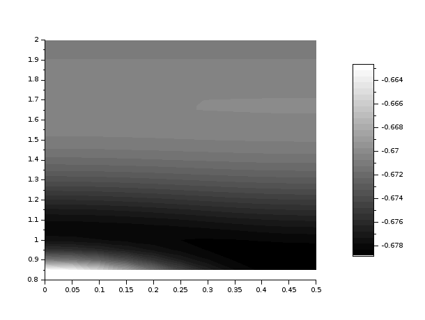
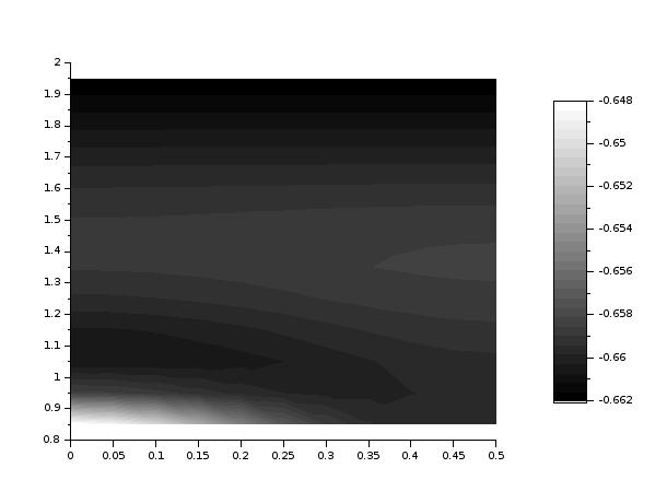
Figure 3. Case (5.1) in two dimensions. Plot of $L\mapsto\min_{\lambda}\mathcal{E}[\lambda L]$ in the fundamental domain $\mathcal{D}$ for $s=6$ (up left), $s=5.3$ (up right), $s=5.15$ (down left) and $s=5.07$ (down right).

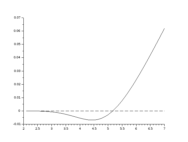
Figure 4. Case (5.1) in two dimensions. Plot of $s\mapsto\min_{\lambda}\mathcal{E}[\lambda\mathbb{Z}^{2}]-\min_{\lambda}\mathcal{E}[\lambda\mathsf{A}_{2}]$ for $s\in[2.1,7]$.

We now replace $\rho$ by a Gaussian function. Namely, we consider the case

$$F(r)=r\log r,\quad\rho(r)=e^{-\delta r^{2}},\quad\phi(r)=\frac{1}{r^{12}}-\frac{1}{r^{6}}.$$ (5.2)

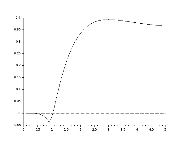
Figure 5. Case (5.2) in two dimensions. Plot of $\delta\mapsto\min_{\lambda}\mathcal{E}[\lambda\mathbb{Z}^{2}]-\min_{\lambda}\mathcal{E}[\lambda\mathsf{A}_{2}]$ for $\delta\in[0.1,5]$.

In this case, the triangular lattice $\lambda_{\mathsf{A}_{2}}^{\mathcal{E}}\mathsf{A}_{2}$ still seems to be minimizing $\mathcal{E}$ for large $\delta$, see Figure 6. More precisely:

• There exists $\delta_{0}\approx 1.04$ such that, for $\delta>\delta_{0}$, the triangular lattice $\lambda_{\mathsf{A}_{2}}^{\mathcal{E}}\mathsf{A}_{2}$ is the global minimizer of $\mathcal{E}$ in $\mathcal{L}_{2}$.

• For $\delta<\delta_{0}$, the global minimizer of $\mathcal{E}$ seems to move (continuously) in $\mathcal{D}$ increasingly following the $y$-axis as $\delta$ decreases to $0$. For instance,

  • If $\delta=1$, then the minimizer is $(0,y_{1})$ where $y_{1}\approx 1.014$.

  • If $\delta=0.95$, then the minimizer is $(0,y_{0.95})$ where $y_{0.95}\approx 1.665$.

• Furthermore, we have checked that, for $\delta>\delta_{0}$,

  $$\min_{\lambda}\mathcal{E}[\lambda\mathbb{Z}^{2}]=\mathcal{E}[\lambda_{\mathbb{Z}^{2}}^{\mathcal{E}}\mathbb{Z}^{2}]>\mathcal{E}[\lambda_{\mathsf{A}_{2}}^{\mathcal{E}}\mathsf{A}_{2}]=\min_{\lambda}\mathcal{E}[\lambda\mathsf{A}_{2}],$$

  whereas the inequality is reversed if $\delta<\delta_{0}$ (see Figure 5).

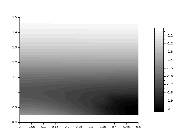
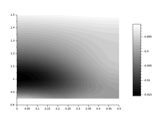
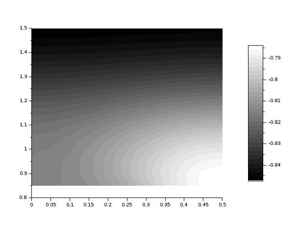
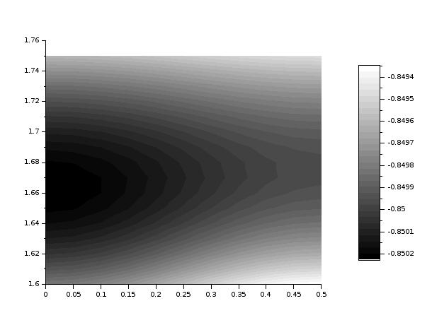
Figure 6. Case (5.2) in two dimensions. Plot of $L\mapsto\min_{\lambda}\mathcal{E}[\lambda L]$ when $\delta=2$ (up left), $\delta=1$ (up right) and $\delta=0.95$ (down left and right) in the fundamental domain $\mathcal{D}$.

5.1.3. Numerical investigation in 3d

Let us go back to case (5.1), now in three dimensions. We investigate the difference of energies between the Simple Cubic (SC), Face-Centered Cubic (FCC), and Body-Centered Cubic (BCC) lattices, namely, $\mathbb{Z}^{3},\mathsf{D}_{3},\mathsf{D}_{3}^{*}$, as $s$ increases. Examples of FCC and BCC metals are Al, Cu, Ag, Au, Ni, Pd, Pt, and Nb, Cr, V, Fe, respectively [37]. Po is the only metal crystallizing in a SC structure [33].

Before giving our numerical results, let us remark that the lattices $\mathbb{Z}^{3}$, $\mathsf{D}_{3}$, and $\mathsf{D}_{3}^{*}$ are critical points of $\mathcal{E}$ in $\mathcal{L}_{3}(1)$. Moreover, recall the following conjectures:

• Sarnak-Strombergsson’s conjecture (see [32, Equation (44)]): for all $s\geq 3/2$ (and in particular for $s>3$, so that $r\mapsto r^{-s}\in\mathcal{S}_{3}^{+}$), $\mathsf{D}_{3}$ is the unique minimizer of $L\mapsto\zeta_{L}(s)$ in $\mathcal{L}_{3}(1)$.

• The global minimizer of the Lennard-Jones energy $E_{\phi}$ is $\lambda_{\mathsf{D}_{3}}^{\phi}\mathsf{D}_{3}$ (see e.g. [40, Figure 5] and [7, Conjecture 1.7]).

We have numerically studied the following function

$$s\mapsto\min_{\lambda>0}\mathcal{E}[\lambda L],\quad L\in\{\mathsf{D}_{3},\mathsf{D}_{3}^{*},\mathbb{Z}^{3}\}$$

for $s>3$, see Figure 7. We have found that there exist $s_{0}<s_{1}<s_{2}$ where $s_{0}\approx 5.4985$, $s_{1}\approx 5.576$, and $s_{2}\approx 5.584$ such that

• For $s\in(3,s_{0})$, $\min_{\lambda>0}\mathcal{E}[\lambda\mathbb{Z}^{3}]<\min_{\lambda>0}\mathcal{E}[\lambda\mathsf{D}_{3}^{*}]<\min_{\lambda>0}\mathcal{E}[\lambda\mathsf{D}_{3}]$;

• For $s\in(s_{0},s_{1})$, $\min_{\lambda>0}\mathcal{E}[\lambda\mathbb{Z}^{3}]<\min_{\lambda>0}\mathcal{E}[\lambda\mathsf{D}_{3}]<\min_{\lambda>0}\mathcal{E}[\lambda\mathsf{D}_{3}^{*}]$;

• For $s\in(s_{1},s_{2})$, $\min_{\lambda>0}\mathcal{E}[\lambda\mathsf{D}_{3}]<\min_{\lambda>0}\mathcal{E}[\lambda\mathbb{Z}^{3}]<\min_{\lambda>0}\mathcal{E}[\lambda\mathsf{D}_{3}^{*}]$;

• For $s>s_{2}$, $\min_{\lambda>0}\mathcal{E}[\lambda\mathsf{D}_{3}]<\min_{\lambda>0}\mathcal{E}[\lambda\mathsf{D}_{3}^{*}]<\min_{\lambda>0}\mathcal{E}[\lambda\mathbb{Z}^{3}]$.

It is remarkable that for small values of $s$ the simple cubic lattice $\mathbb{Z}^{3}$ has lower energy with respect to the usually energetically favored $\mathsf{D}_{3}$ and $\mathsf{D}_{3}^{*}$.

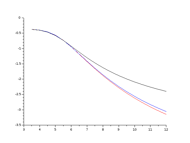
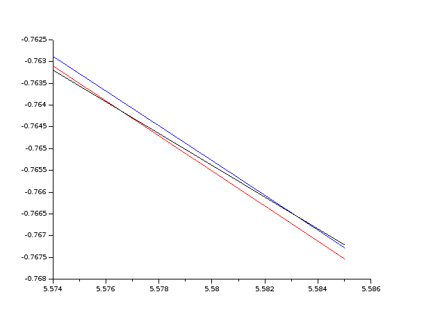
Figure 7. Case (5.1) in three dimensions. Plots of $s\mapsto\min_{\lambda}\mathcal{E}[\lambda L]$ for $L=\mathsf{D}_{3}$ (red), $L=\mathsf{D}_{3}^{*}$ (blue) and $L=\mathbb{Z}^{3}$ (black) on two different intervals.

Consider now the Gaussian case (5.2) in three dimensions. The total energy then reads

$$\mathcal{E}[L]:=\theta_{L}(\delta)\log\theta_{L}(\delta)+\zeta_{L}(12)-\zeta_{L}(6),\quad\textnormal{where}\quad\theta_{L}(\delta):=\sum_{p\in L\backslash\{0\}}e^{-\delta|p|^{2}}.$$

In the following, we will call $\theta_{L}(\delta)$ the lattice theta function with parameter $\delta>0$. Note however that under this name one usually refers to such sum including the term for $p=0$ and with weight $e^{-\delta\pi|p|^{2}}$.

We recall the following conjectures:

• Sarnak-Strombergsson’s conjecture (see [32, Equation (43)]): if $\delta<\pi$, then $\mathsf{D}_{3}^{*}$ minimizes $L\mapsto\theta_{L}(\delta)$ in $\mathcal{L}_{3}(1)$. If $\delta>\pi$, then $\mathsf{D}_{3}$ minimizes the same lattice theta function in $\mathcal{L}_{3}(1)$ (with a coexistence phase around $\pi$ actually).

• As mentioned before, the unique minimizer of the Lennard-Jones energy $E_{\phi}$ in $\mathcal{L}_{3}$ is $\lambda_{\mathsf{D}_{3}}^{\phi}\mathsf{D}_{3}$ (see e.g. [7] and [40, Figure 5]).

In Figure 8 we plot the functions $\delta\mapsto\min_{\lambda>0}\mathcal{E}[\lambda L]$ for $L\in\{\mathsf{D}_{3},\mathsf{D}_{3}^{*},\mathbb{Z}^{3}\}$. We numerically observe that there exist $0<\delta_{1}<\delta_{2}<\delta_{3}$, where $\delta_{1}\approx 1.13$, $\delta_{2}\approx 1.21$, and $\delta_{3}\approx 1.223$ such that

• for all $\delta\in(0,\delta_{1})$, $\min_{\lambda>0}\mathcal{E}[\lambda\mathbb{Z}^{3}]<\min_{\lambda>0}\mathcal{E}[\lambda\mathsf{D}_{3}^{*}]<\min_{\lambda>0}\mathcal{E}[\lambda\mathsf{D}_{3}]$;

• for all $\delta\in(\delta_{1},\delta_{2})$, $\min_{\lambda>0}\mathcal{E}[\lambda\mathbb{Z}^{3}]<\min_{\lambda>0}\mathcal{E}[\lambda\mathsf{D}_{3}]<\min_{\lambda>0}\mathcal{E}[\lambda\mathsf{D}_{3}^{*}]$;

• for all $\delta\in(\delta_{2},\delta_{3})$, $\min_{\lambda>0}\mathcal{E}[\lambda\mathsf{D}_{3}]<\min_{\lambda>0}\mathcal{E}[\lambda\mathbb{Z}^{3}]<\min_{\lambda>0}\mathcal{E}[\lambda\mathsf{D}_{3}^{*}]$;

• for all $\delta>\delta_{3}$, $\min_{\lambda>0}\mathcal{E}[\lambda\mathsf{D}_{3}]<\min_{\lambda>0}\mathcal{E}[\lambda\mathsf{D}_{3}^{*}]<\min_{\lambda>0}\mathcal{E}[\lambda\mathbb{Z}^{3}]$.

It is indeed important that the EAM energy favors $\mathsf{D}_{3}$ or $\mathsf{D}_{3}^{*}$ for some specific choice of parameters. In fact, FCC and BCC lattices are commonly emerging in metals. It is also remarkable that the simple cubic lattice $\mathbb{Z}^{3}$ (up to rescaling) is favored with respect to $\mathsf{D}_{3}$ or $\mathsf{D}_{3}^{*}$ for some other choice of parameters. In [7], we were able to identify a range of densities such that cubic lattices are locally optimal at fixed density, but it is the first time – according to our knowledge – that such phenomenon is observed at the level of the global minimizer.

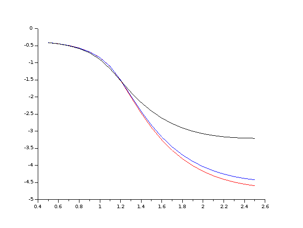
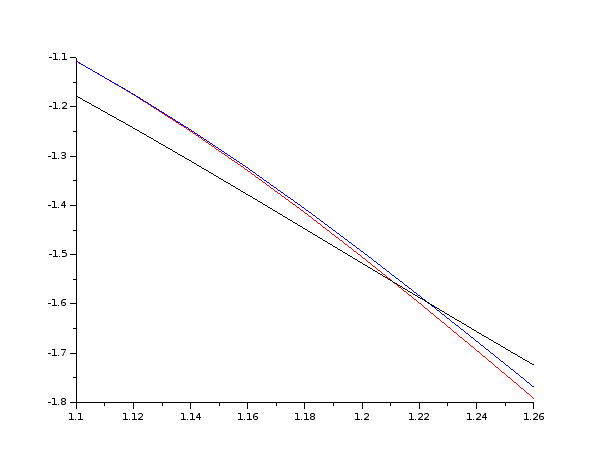
Figure 8. Case (5.2) in three dimensions. Plot of $\delta\mapsto\min_{\lambda}\mathcal{E}[\lambda L]$ for $L=\mathsf{D}_{3}$ (red), $L=\mathsf{D}_{3}^{*}$ (blue) and $L=\mathbb{Z}^{3}$ (black) on two different intervals.

5.2. The power-law case $F(r)=r^{t}$

In this subsection, we study the case where $F(r)=r^{t}$, $t>0$. Although $F$ is not a one-well potential, this case turns out to be mathematically interesting. Indeed, we are able to present a special case where we can explicitly compute $\min_{\lambda}\mathcal{E}[\lambda L]$ for any $L\in\mathcal{L}_{d}(1)$. As we have seen above, this dimension reduction is extremely helpful when one looks for the ground state of $\mathcal{E}$ in $\mathcal{L}_{d}$, especially for $d=2$, since we can plot $L\mapsto\min_{\lambda}\mathcal{E}[\lambda L]$ in the fundamental domain $\mathcal{D}$.

5.2.1. A special power-law case

Let us now assume that

$$F(r)=r^{t},\quad\rho(r)=r^{-s},\quad\phi(r)=ar^{-\alpha}-br^{-\beta},$$

for $t>0$, $s>d$, $\alpha>\beta>d$, and $a,\,b>0$. Therefore, by (2.3) we have, for any $\lambda>0$ and any $L\in\mathcal{L}_{d}(1)$, that

$$\mathcal{E}[\lambda L]=\lambda^{-st}\zeta_{L}(s)^{t}+a\lambda^{-\alpha}\zeta_{L}(\alpha)-b\lambda^{-\beta}\zeta_{L}(\beta).$$

For a fixed lattice $L$, the critical points of $\lambda\mapsto\mathcal{E}[\lambda L]$ are the solutions of the following equation

$$b\beta\zeta_{L}(\beta)\lambda^{st+\alpha}-st\zeta_{L}(s)^{t}\lambda^{\alpha+\beta}-a\alpha\zeta_{L}(\alpha)\lambda^{st+\beta}=0.$$ (5.3)

Solving this equation in closed form is impracticable out of a discrete set of parameter values. Correspondingly, comparing energy values is even more complicated than in the pure Lennard-Jones-type case, which is already challenging when treated in whole generality.

Having pointed out this difficulty, we now focus on some additional specifications of the parameters, allowing to proceed further with the analysis. We have the following.

Theorem 5.4 (Special power-law case).

Let $\alpha,\beta,s$, and $t$ such that

$$d<s,\quad d<\beta<st<\alpha,\quad\textnormal{and}\quad\alpha=2st-\beta.$$ (5.4)

Then, $\lambda^{\mathcal{E}}_{L}$ exists for all $L\in\mathcal{L}_{d}(1)$. Moreover, $\lambda^{\mathcal{E}}_{L_{d}}L_{d}$ is a global minimizer in $\mathcal{L}_{d}$ of $\mathcal{E}$, now reading

$$\mathcal{E}[L]=\zeta_{L}(s)^{t}+a\zeta_{L}(\alpha)-b\zeta_{L}(\beta),$$

if and only if $L_{d}$ is a minimizer in $\mathcal{L}_{d}(1)$ of

$$e_{*}(L): =-\frac{\displaystyle C_{1}\frac{\zeta_{L}(s)^{2t}}{\zeta_{L}(\beta)}+C_{2}\zeta_{L}(s)^{t}\sqrt{c_{1}\frac{\zeta_{L}(s)^{2t}}{\zeta_{L}(\beta)^{2}}+c_{2}\frac{\zeta_{L}(\alpha)}{\zeta_{L}(\beta)}}+C_{3}\zeta_{L}(\alpha)}{\displaystyle\left(\sqrt{c_{1}}\frac{\zeta_{L}(s)^{t}}{\zeta_{L}(\beta)}+\sqrt{c_{1}\frac{\zeta_{L}(s)^{2t}}{\zeta_{L}(\beta)^{2}}+c_{2}\frac{\zeta_{L}(\alpha)}{\zeta_{L}(\beta)}}\right)^{\frac{\alpha}{\alpha-st}}},$$

where $C_{i},c_{j}$, $i\in\{1,2,3\}$, $j\in\{1,2\}$, are positive constants defined by

$$C_{1}:=\frac{st}{2b\beta}\left(\frac{st}{\beta}-1\right),\quad C_{2}:=\frac{st}{\beta}-1,\quad C_{3}:=a\left(\frac{\alpha}{\beta}-1\right),\quad c_{1}:=\frac{s^{2}t^{2}}{4b^{2}\beta^{2}},\quad c_{2}:=\frac{a\alpha}{b\beta}.$$ (5.5)

Proof.

For any $L\in\mathcal{L}_{d}(1)$, any critical point of $\lambda\mapsto\mathcal{E}[\lambda L]$ satisfies (see (5.3))

$$\lambda^{st+\beta}\left(b\beta\zeta_{L}(\beta)\lambda^{\alpha-\beta}-st\zeta_{L}(s)^{t}\lambda^{\alpha-st}-a\alpha\zeta_{L}(\alpha)\right)=0.$$

Since $\lambda>0$, by writing $X=\lambda^{\alpha-st}$ and using (5.4) we want to solve

$$b\beta\zeta_{L}(\beta)X^{2}-st\zeta_{L}(s)^{t}X-a\alpha\zeta_{L}(\alpha)=0,\quad X>0,$$

for which the unique solution is

$$X=\frac{st\zeta_{L}(s)^{t}+\sqrt{s^{2}t^{2}\zeta_{L}(s)^{2t}+4ab\alpha\beta\zeta_{L}(\alpha)\zeta_{L}(\beta)}}{2b\beta\zeta_{L}(\beta)}.$$

Since $\alpha-st>0$ and $b\beta\zeta_{L}(\beta)>0$, we find that the critical point is a minimizer and thus coincides with $\lambda^{\mathcal{E}}_{L}$ defined in (2.6). More precisely, we have

$$\lambda^{\mathcal{E}}_{L}=\left(\frac{st\zeta_{L}(s)^{t}+\sqrt{s^{2}t^{2}\zeta_{L}(s)^{2t}+4ab\alpha\beta\zeta_{L}(\alpha)\zeta_{L}(\beta)}}{2b\beta\zeta_{L}(\beta)}\right)^{\frac{1}{\alpha-st}}.$$

We hence get, for any $L\in\mathcal{L}_{d}(1)$, that

$$\min_{\lambda}\mathcal{E}[\lambda L]=\mathcal{E}[\lambda^{\mathcal{E}}_{L}L]$$

$$=(\lambda^{\mathcal{E}}_{L})^{-st}\zeta_{L}(s)^{t}+a(\lambda^{\mathcal{E}}_{L})^{-\alpha}\zeta_{L}(\alpha)-b(\lambda^{\mathcal{E}}_{L})^{-\beta}\zeta_{L}(\beta)$$

$$=(\lambda^{\mathcal{E}}_{L})^{-\alpha}\left\{\zeta_{L}(s)^{t}(\lambda^{\mathcal{E}}_{L})^{\alpha-st}-b\zeta_{L}(\beta)(\lambda^{\mathcal{E}}_{L})^{\alpha-\beta}+a\zeta_{L}(\alpha)\right\}$$

$$=(\lambda^{\mathcal{E}}_{L})^{-\alpha}\left\{\zeta_{L}(s)^{t}(\lambda^{\mathcal{E}}_{L})^{\alpha-st}-\frac{st\zeta_{L}(s)^{t}(\lambda^{\mathcal{E}}_{L})^{\alpha-st}+a\alpha\zeta_{L}(\alpha)}{\beta}+a\zeta_{L}(\alpha)\right\}$$

$$=(\lambda^{\mathcal{E}}_{L})^{-\alpha}\left\{\zeta_{L}(s)^{t}\left(1-\frac{st}{\beta}\right)(\lambda^{\mathcal{E}}_{L})^{\alpha-st}+a\zeta_{L}(\alpha)\left(1-\frac{\alpha}{\beta}\right)\right\}$$

$$=(\lambda^{\mathcal{E}}_{L})^{-\alpha}\left\{\zeta_{L}(s)^{t}\left(1-\frac{st}{\beta}\right)\left(\frac{st\zeta_{L}(s)^{t}+\sqrt{s^{2}t^{2}\zeta_{L}(s)^{2t}+4ab\alpha\beta\zeta_{L}(\alpha)\zeta_{L}(\beta)}}{2b\beta\zeta_{L}(\beta)}\right)+a\zeta_{L}(\alpha)\left(1-\frac{\alpha}{\beta}\right)\right\}$$

$$=(\lambda^{\mathcal{E}}_{L})^{-\alpha}\left\{\frac{st}{2b\beta}\left(1-\frac{st}{\beta}\right)\frac{\zeta_{L}(s)^{2t}}{\zeta_{L}(\beta)}+\left(1-\frac{st}{\beta}\right)\zeta_{L}(s)^{t}\sqrt{\frac{s^{2}t^{2}\zeta_{L}(s)^{2t}}{4b^{2}\beta^{2}\zeta_{L}(\beta)^{2}}+\frac{a\alpha\zeta_{L}(\alpha)}{b\beta\zeta_{L}(\beta)}}+a\left(1-\frac{\alpha}{\beta}\right)\zeta_{L}(\alpha)\right\},$$

where in the fourth line we have used the fact that $\lambda^{\mathcal{E}}_{L}$ is a critical point of $\lambda\mapsto\mathcal{E}[\lambda L]$, i.e., $b\beta\zeta_{L}(\beta)(\lambda^{\mathcal{E}}_{L})^{\alpha-\beta}-st\zeta_{L}(s)^{t}(\lambda^{\mathcal{E}}_{L})^{\alpha-st}-a\alpha\zeta_{L}(\alpha)=0$. Note that by assumption we have

$$1-\frac{st}{\beta}<0,\quad 1-\frac{\alpha}{\beta}<0.$$

It follows that, defining the positive constants $C_{i},c_{j}$, $i\in\{1,2,3\}$, $j\in\{1,2\}$, as in (5.5), that

$$\min_{\lambda}\mathcal{E}[\lambda L] =-(\lambda^{\mathcal{E}}_{L})^{-\alpha}\left\{C_{1}\frac{\zeta_{L}(s)^{2t}}{\zeta_{L}(\beta)}+C_{2}\zeta_{L}(s)^{t}\sqrt{c_{1}\frac{\zeta_{L}(s)^{2t}}{\zeta_{L}(\beta)^{2}}+c_{2}\frac{\zeta_{L}(\alpha)}{\zeta_{L}(\beta)}}+C_{3}\zeta_{L}(\alpha)\right\}$$

$$=-\frac{\displaystyle C_{1}\frac{\zeta_{L}(s)^{2t}}{\zeta_{L}(\beta)}+C_{2}\zeta_{L}(s)^{t}\sqrt{c_{1}\frac{\zeta_{L}(s)^{2t}}{\zeta_{L}(\beta)^{2}}+c_{2}\frac{\zeta_{L}(\alpha)}{\zeta_{L}(\beta)}}+C_{3}\zeta_{L}(\alpha)}{\displaystyle\left(\sqrt{c_{1}}\frac{\zeta_{L}(s)^{t}}{\zeta_{L}(\beta)}+\sqrt{c_{1}\frac{\zeta_{L}(s)^{2t}}{\zeta_{L}(\beta)^{2}}+c_{2}\frac{\zeta_{L}(\alpha)}{\zeta_{L}(\beta)}}\right)^{\frac{\alpha}{\alpha-st}}},$$

which completes the proof. ∎

5.2.2. Numerical investigations of the special power-law case in 2d and 3d

We let $t\in(0,9/d)$ vary and fix

$$a=b=1,\quad\alpha=12,\quad\beta=6,\quad s=9/t,$$

so that

$$F(r)=r^{t},\quad\rho(r)=r^{-{9}/{t}},\quad\phi(r)=\frac{1}{r^{12}}-\frac{1}{r^{6}}.$$ (5.6)

Note that (5.4) holds under these assumptions. In two dimensions, by testing as $t\in(0,4.5)$ increases, we observe numerically the following:

• If $t\in(0,t_{1})$, $t_{1}\approx 1.605$, then $\mathsf{A}_{2}$ minimizes $e_{*}$ (see Figures 9 and 10);

• If $t\in(t_{1},t_{2})$, where $t_{2}\approx 1.633$, then $\mathbb{Z}^{2}$ is a local minimizer of $e_{*}$ but there seems to be no minimizer for $e_{*}$ (see Figure 11);

• if $t\in(t_{2},4.5)$, there seems to be no minimizer for $e_{*}$, and $\mathbb{Z}^{2}$ is a saddle point (see Figure 12).

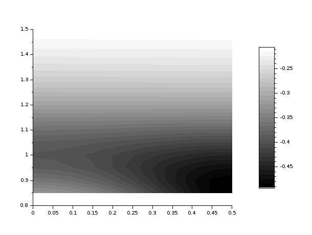
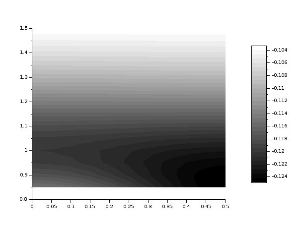
Figure 9. Special power-law case (5.6) in two dimensions. Plot of $e_{*}$ on the fundamental domain $\mathcal{D}$. For $t=1$ (left) and $t=1.5$ (right), the minimizer of $e_{*}$ is the triangular lattice $\mathsf{A}_{2}$ given by the point $(1/2,\sqrt{3}/2)$.

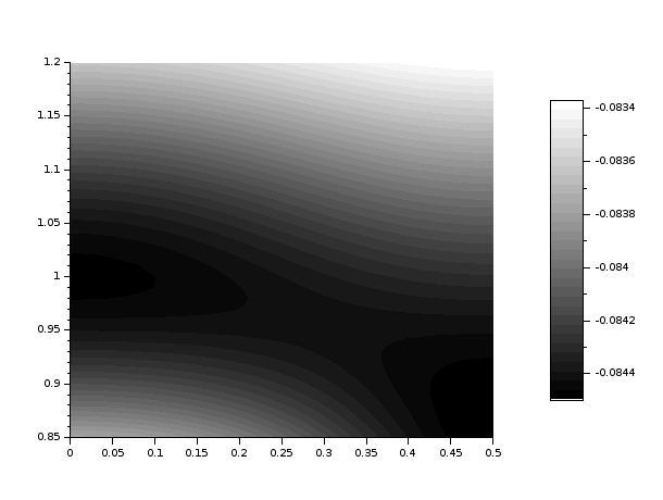
Figure 10. Special power-law case (5.6) in two dimensions. Plot of $e_{*}$ on the fundamental domain $\mathcal{D}$ for $t=1.605$. The triangular lattice is the global minimizer of $e_{*}$ whereas $\mathbb{Z}^{2}$ (given by the point $(0,1)$) is a local minimizer.

Similarly to the discussion of Subsection 5.1, for some choice of parameters, a square lattice seems to be locally minimizing the EAM energy, at least within the range of our numerical testing. In [6], we have identified a range of densities for which a square lattice is optimal at fixed density. This seems however to be the first occurrence of such minimality among all possible lattices, without a density constraint. Indeed, when minimizing among all lattices, the square lattice $\mathbb{Z}^{2}$ usually happens to be a saddle point, see, e.g., Figure 1 for the Lennard-Jones case.

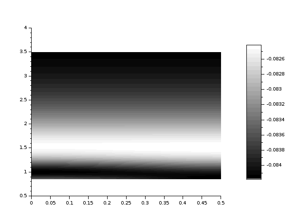
Figure 11. Special power-law case (5.6) in two dimensions. Plot of $e_{*}$ on the fundamental domain $\mathcal{D}$ for $t=1.606$. The square lattice is a local minimizer of $e_{*}$ which does not have any global minimizer. Still, $\mathsf{A}_{2}$ is a local minimizer.

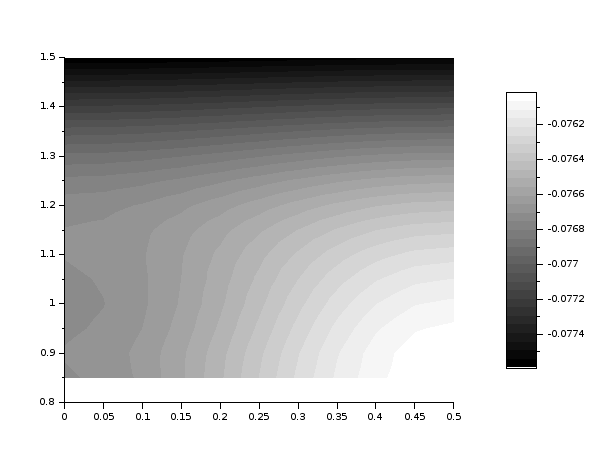
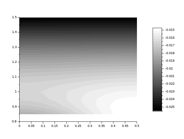
Figure 12. Special power-law case (5.6) in two dimensions. Plot of $e_{*}$ on the fundamental domain $\mathcal{D}$. For $t=1.632$ (left) the square lattice is a local minimizer of $e_{*}$ whereas $\mathsf{A}_{2}$ is a local maximizer. For $t=2$ (right) it seems that $e_{*}$ does not have any local minimizer and $\mathsf{A}_{2}$ stays a local maximizer. In both cases, there is no global minimum.

We have numerically investigated the three-dimensional case as well, comparing the energies of $L\in\{\mathbb{Z}^{3},\mathsf{D}_{3},\mathsf{D}_{3}^{*}\}$. Figure 13 illustrates the numerical results. We observe that there exist $t_{1},t_{2},t_{3}$, where $t_{1}\approx 1.5505$, $t_{2}\approx 1.5515$, and $t_{3}\approx 1.5647$ such that:

• If $t\in(0,t_{1})$, $e_{*}(\mathsf{D}_{3})<e_{*}(\mathsf{D}_{3}^{*})<e_{*}(\mathbb{Z}^{3})$;

• If $t\in(t_{1},t_{2})$, $e_{*}(\mathsf{D}_{3})<e_{*}(\mathbb{Z}^{3})<e_{*}(\mathsf{D}_{3}^{*})$;

• If $t\in(t_{2},t_{3})$, $e_{*}(\mathbb{Z}^{3})<e_{*}(\mathsf{D}_{3})<e_{*}(\mathsf{D}_{3}^{*})$;

• If $t\in(t_{3},3)$, $e_{*}(\mathbb{Z}^{3})<e_{*}(\mathsf{D}_{3}^{*})<e_{*}(\mathsf{D}_{3})$.

When $t\to 0$, since $s=9/t\to\infty$ and $r^{t}\to 1$ for fixed $r>0$, it is expected that the global minimizer of $\mathcal{E}$ in $\mathcal{L}_{3}$ converges to the one of $E_{\phi}$, which in turn is expected to be a FCC lattice. This is supported by our numerics for $t<t_{1}$.

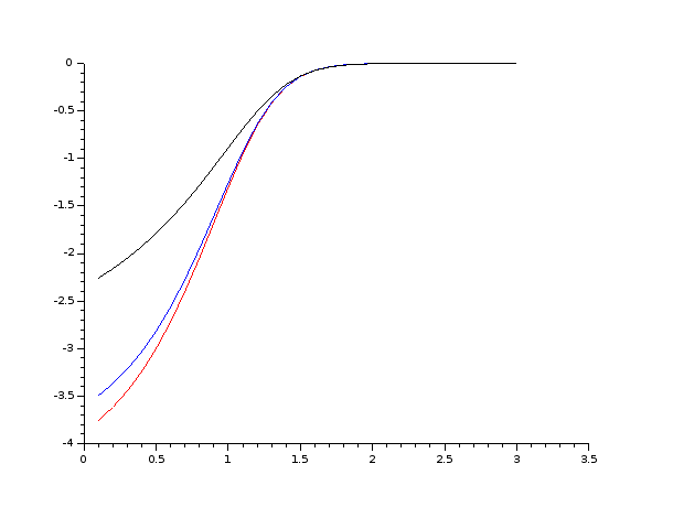
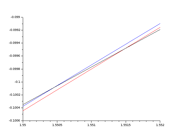
Figure 13. Special power-law case (5.6) in three dimensions. Plot of $t\mapsto e_{*}(L)$ for $L=\mathsf{D}_{3}$ (red), $L=\mathsf{D}_{3}^{*}$ (blue) and $L=\mathbb{Z}^{3}$ (black) for $t\in(0,3)$. The graph on the right is a close-up of the two transitions at $t_{1}$ and $t_{2}$.

References

- [1]
- [2] A. Banerjea and J. R. Smith. Origins of the universal binding-energy relation. Phys. Rev. B, 37(12):6632–6645, 1988.
- [3] M. I. Baskes. Many-body effects in fcc metals: a Lennard-Jones embedded-atom potential. Phys. Rev. Lett., 83(13):2592–2595, 1983.
- [4] M. I. Baskes. Application of the Embedded-Atom Method to covalent materials: a semiempirical potential for silicon. Phys. Rev. Lett., 59(23):2666–2669, 1987.
- [5] L. Bétermin. Two-dimensional Theta Functions and crystallization among Bravais lattices. SIAM J. Math. Anal., 48(5):3236–3269, 2016.
- [6] L. Bétermin. Local variational study of 2d lattice energies and application to Lennard-Jones type interactions. Nonlinearity, 31(9):3973–4005, 2018.
- [7] L. Bétermin. Local optimality of cubic lattices for interaction energies. Anal. Math. Phys., 9(1):403–426, 2019.
- [8] L. Bétermin. Minimizing lattice structures for Morse potential energy in two and three dimensions. J. Math. Phys., 60(10):102901, 2019.
- [9] L. Bétermin. Effect of periodic arrays of defects on lattice energy minimizers. Preprint. arXiv:2008.00676, 2020.
- [10] L. Bétermin and M. Petrache. Optimal and non-optimal lattices for non-completely monotone interaction potentials. Anal. Math. Phys., 9(4):2033–2073, 2019.
- [11] L. Bétermin and P. Zhang. Minimization of energy per particle among Bravais lattices in : Lennard-Jones and Thomas-Fermi cases. Commun. Contemp. Math., 17(6):1450049, 2015.
- [12] X. Blanc and C. Le Bris. Periodicity of the infinite-volume ground state of a one-dimensional quantum model. Nonlinear Anal., 48(6):791–803, 2002.
- [13] X. Blanc and M. Lewin. The Crystallization Conjecture: a review. EMS Surv. Math. Sci., 2:255–306, 2015.
- [14] J. Cai and Y. Y. Ye. Simple analytical embedded-atom-potential model including a long-range force for fcc metals and their alloys. Phys. Rev. B, 54(12):8398–8410, 1996.
- [15] H. Cohn and A. Kumar. Universally optimal distribution of points on spheres. J. Amer. Math. Soc., 20(1):99–148, 2007.
- [16] H. Cohn, A. Kumar, S. D. Miller, D. Radchenko, and M. Viazovska. Universal optimality of the and Leech lattices and interpolation formulas. Preprint. arXiv:1902:05438, 2019.
- [17] M. S. Daw and M. I. Baskes. Semiempirical, Quantum Mechanical Calculation of Hydrogen Embrittlement in Metals. Phys. Rev. Lett., 50(17):1285–1288, 1983.
- [18] M. S. Daw and M. I. Baskes. Embedded-atom method: Derivation and application to impurities, surfaces and other defects in metals. Phys. Rev. B, 29(12):6443–6453, 1984.
- [19] M. S. Daw, S. M. Foiles, and M. I. Baskes. The embedded-atom method: a review of theory and applications. Materials Science Reports, 9(7-8):251–310, 1993.
- [20] J. Dorrell and L. B. Pártay. Pressure-temperature phase diagram of lithium, predicted by Embedded Atom Model potentials. J. Phys. Chem. B, 124:6015–6023, 2020.
- [21] M. W. Finnis and J. E. Sinclair. A simple empirical n-body potential for transition metals. Philosophical Magazine A, 50(1):45–55, 1984.
- [22] S. Foiles. Embedded-Atom and related methods for modeling metallic mystems. MRS Bulletin, 21(2):24–28, 1996.
- [23] G. Grochola, S. P. Russo, and I. K. Snook On fitting a gold embedded atom method potential using the force matching method. J. Chem. Phys., 123:204719, 2005.
- [24] A. Hernandez, A. Balasubramanian, F. Yuan et al. Fast, accurate, and transferable many-body interatomic potentials by symbolic regression. npj Comput Mater, 5:112, 2019.
- [25] J. E. Jaffe, R. J. Kurtz, and M. Gutowski. Comparison of embedded-atom models and first-principles calculations for Al phase equilibrium. Computational Materials Science, 18(2):199–204, 2000.
- [26] R. A. Johnson. Alloy models with the embedded-atom method. Phys. Rev. B, 39, 12554, 1989.
- [27] R. A. Johnson and D. J. Oh. Analytic embedded atom method model for bcc metals. J. Mater. Res., 4(5):1195–1201, 1989.
- [28] R. LeSar. Introduction to Computational Materials Science. Fundamentals to Applications. Cambridge University Press, 2013.
- [29] H. L. Montgomery. Minimal Theta functions. Glasg. Math. J., 30(1):75–85, 1988.
- [30] C. Poole. Encyclopedic Dictionary of Condensed Matter Physics. Elsevier, 1st edition edition, 2004.
- [31] J. H. Rose, J. R. Smith, F. Guinea, and J. Ferrante. Universal features of the equation of state of metals. Phys. Rev. B, 29(6):2963–2969, 1984.
- [32] P. Sarnak and A. Strömbergsson. Minima of Epstein’s Zeta Function and heights of flat tori. Invent. Math., 165:115–151, 2006.
- [33] A. Silva and J. van Wezel. The simple-cubic structure of elemental Polonium and its relation to combined charge and orbital order in other elemental chalcogens. SciPost Phys., 4 (2018), 028.
- [34] S. G. Srinivasan and M. I. Baskes. On the Lennard-Jones EAM potential. Proc. R. Soc. London, Ser. A, 460:1649–1672, 2004.
- [35] A. P. Sutton and J. Chen. Long-range Finnis-Sinclair potentials. Philosophical Magazine Letters, 61(3):139–146, 1990.
- [36] A. Terras. Harmonic analysis on symmetric spaces and applications II. Springer New York, 1988.
- [37] A. F. Wells. Structural Inorganic Chemistry. Clarendon Press, Oxford, 1975.
- [38] X.-J. Yuan, N.-X. Chen, and J. Shen. Construction of embedded-atom-method interatomic potentials for alkaline metals (Li, Na, and K) by lattice inversion Chin. Phys. B, 21(5):053401, 2012
- [39] Y. Zhang, C. Hu, and B. Jiang. Embedded-atom neural network potentials: efficient and accurate machine learning with a physically inspired representation J. Phys. Chem. Lett., 10(17):4962-4967, 2019
- [40] M. Zschornak, T. Leisegang, F. Meutzner, H. Stöcker, T. Lemser, T. Tauscher, C. Funke, C. Cherkouk, and D. C. Meyer. Harmonic principles of elemental crystals — from atomic interaction to fundamental symmetry. Symmetry, 10(6):228, 2018.