Local classical MAX-CUT algorithm outperforms p=2p=2 QAOA on high-girth regular graphs

Kunal Marwaha OrcID: 0000-0001-9084-6971 Email: marwahaha@berkeley.edu Affiliation: Berkeley Center for Quantum Information and Computation, University of California, Berkeley, California 94720, USA
Abstract

The pp-stage Quantum Approximate Optimization Algorithm (QAOAp) is a promising approach for combinatorial optimization on noisy intermediate-scale quantum (NISQ) devices, but its theoretical behavior is not well understood beyond p=1p=1. We analyze QAOA2 for the maximum cut problem (MAX-CUT), deriving a graph-size-independent expression for the expected cut fraction on any DD-regular graph of girth >5>5 (i.e. without triangles, squares, or pentagons).

We show that for all degrees D2D\geq 2 and every DD-regular graph GG of girth >5>5, QAOA2 has a larger expected cut fraction than QAOA1 on GG. However, we also show that there exists a 22-local randomized classical algorithm AA such that AA has a larger expected cut fraction than QAOA2 on all GG. This supports our conjecture that for every constant pp, there exists a local classical MAX-CUT algorithm that performs as well as QAOAp on all graphs.

1 Introduction

The pp-stage Quantum Approximate Optimization Algorithm (QAOAp) [FGG14] is a protocol to use near-term quantum computers for combinatorial optimization [Pre18]. The number pp is called the algorithm’s depth, with small values of pp realizable on current devices [AAB+20] [ZWC+20], often called noisy intermediate-scale quantum (NISQ) devices. The performance of the algorithm is difficult to analyze, even for small values of pp and in restricted settings [FGG14] [WL20]. In this work we analyze QAOA2 for the maximum cut problem (MAX-CUT) and compare it with local classical algorithms. There is a classical algorithm (the Goemans-Williamson semidefinite program [GW95]) that, under certain computational complexity assumptions, achieves the optimal worst-case approximation ratio for MAX-CUT among all polynomial-time classical and quantum algorithms [Kho02].aa a Specifically, this holds assuming Khot’s Unique Games Conjecture and the widely-believed conjecture that 𝐍𝐏𝐁𝐐𝐏{\mathbf{NP}\not\subseteq\mathbf{BQP}}. However, this is a worst-case ratio; there may be inputs where QAOAp outperforms the Goemans-Williamson program. Moreover, the Goemans-Williamson program is a global algorithm, for which the assignment of each vertex depends on the entire graph; by contrast, QAOAp is a pp-local algorithm, where the assignment depends only on the vertex’s radius pp neighborhood. Does there exist a local classical algorithm that performs as well as QAOAp on every graph? In this work we answer this question positively for p=2p=2 on regular graphs of girth above 5.

1.1 Related work

QAOA is thought to be competitive with classical approximation algorithms. Initially, QAOA1 was the best known approximate algorithm for MAX-3-LIN-2 [FGG15], although an improved classical algorithm was quickly found [BMO+15]. For MAX-CUT, QAOA1 guarantees an expected cut fraction of >12+0.3032D>\frac{1}{2}+\frac{0.3032}{\sqrt{D}} on triangle-free DD-regular graphs [WHJR18], outperforming the lower bound of the best known local classical algorithm, the threshold algorithm [HRSS14]. However, a direct calculation by Hastings [Has19] shows that this lower bound is not tight: The threshold algorithm with optimal parameter value outperforms QAOA1 on triangle-free DD-regular graphs for all but 44 choices of 2D<10002\leq D<1000, and likely for all larger DD. Hastings also introduces a family of local classical optimization algorithms, identifying algorithms from this family that outperform QAOA1 for each of the remaining 44 choices of DD.

QAOA has very few proven results about its performance, and QAOAp’s optimal parameters are only known for small pp or for severely restricted problems. [WHJR18] derives a graph-size-independent expression of the expected cut fraction for QAOA1 on any graph, determining the maximum for any triangle-free DD-regular graph. [WHJR18] and [Sze19] use separate approaches to derive the expected and maximum expected cut fraction for QAOA2 on any 22-regular graph. [WL20] shows that QAOA2 has a maximum expected cut fraction of approximately 0.75590.7559 on 33-regular graphs. For larger pp, the creators of QAOA have proposed a hybrid algorithm to find optimal parameters, alternating between the quantum circuit and a classical parameter optimizer; unfortunately, this approach involves non-convex classical optimization, making its runtime difficult to analyze [MRBAG16].

1.2 Our results

This work studies QAOA2 and local classical algorithms for MAX-CUT on DD-regular graphs of girth >5>5. We derive a graph-size-independent expression for the expected cut fraction of QAOA2 on these graphs. We numerically optimize this expression over QAOA’s input parameters to find the maximum expected cut fraction for each D<500D<500. We then generalize the 11-local threshold algorithm with one parameter τ\tau to the nn-step threshold algorithm, an nn-local algorithm with nn parameters (τ1,,τn)(\tau_{1},\cdots,\tau_{n}). We derive the performance of the 22-step threshold algorithm on these graphs as a function of (τ1,τ2)(\tau_{1},\tau_{2}). When τ1=τ2\tau_{1}=\tau_{2}, a direct calculation shows that the optimal 22-step threshold algorithm outperforms QAOA2 for all 41<D<50041<D<500, and likely for all larger DD based on asymptotic behavior. Another direct calculation on D<50D<50 shows that the optimal 22-step threshold algorithm outperforms QAOA2 for all 5<D<505<D<50. We identify the 22-step threshold algorithm with the family of 2-local classical algorithms in [Has19], specifying instances that outperform QAOA2 for the remaining 4 choices. This shows that for all D2D\geq 2, there is a 22-local classical MAX-CUT algorithm that outperforms QAOA2 on all DD-regular graphs of girth above 5.

Why the restriction on girth? This condition massively simplifies the analysis of local algorithms. Consider an \ell-local algorithm, where a vertex’s assignment depends on its radius \ell neighborhood. When girth >2+1>2\ell+1, the neighborhood looks like a tree. Previous analyses of QAOA1 and the 1-step threshold algorithm use this property when studying triangle-free graphs (i.e. girth >3>3). Similarly, our analysis of QAOA2 and the 2-step threshold algorithm considers graphs of girth above 55 (no triangles, squares, or pentagons). Our analysis could be extended beyond =2\ell=2; we suspect that the pp-step threshold algorithm performs as well as QAOAp on every graph of girth >2p+1>2p+1.

2 QAOA2 performance on MAX-CUT

Given a combinatorial problem on a graph G(V,E)G(V,E), QAOA is an algorithm on |V||V| qubits, where each vertex in GG corresponds to a qubit. QAOA involves two Hamiltonians: the mixing Hamiltonian J=iVσixJ=\sum_{i\in V}\sigma_{i}^{x} and the problem Hamiltonian CC, where each eigenstate of CC encodes a possible solution scored by its eigenvalue. The algorithm approximates adiabatic evolution from the maximal eigenstate of JJ to the maximal eigenstate of CC, the optimal solution. Precisely, QAOAp takes 2p2p parameters (γ1,β1,,γp,βp)(\gamma_{1},\beta_{1},\cdots,\gamma_{p},\beta_{p}) and evolves the initial state ρ0=iV(I/2+σix/2)\rho_{0}=\bigotimes_{i\in V}(I/2+\sigma_{i}^{x}/2) with a unitary U=eiβpJeiγpCeiβ1Jeiγ1CU=e^{-i\beta_{p}J}e^{-i\gamma_{p}C}\cdots e^{-i\beta_{1}J}e^{-i\gamma_{1}C}. The state is then measured in the eigenbasis of CC, which gives an approximate solution. More information on QAOA can be found in [FGG14] and [WHJR18].

For MAX-CUT, let C=(u,v)ECuvC=\sum_{(u,v)\in E}C_{uv} where Cuv=0.5(1σuzσvz)C_{uv}=0.5(1-\sigma_{u}^{z}\sigma_{v}^{z}). The maximal eigenvalue of CC is the maximum number of edges that can be cut on the graph GG; an edge is “cut” if the qubits corresponding to its vertices do not agree when measured in the zz-basis. The expected number of edges cut by QAOA is Tr[CUρ0U]=(u,v)ETr[ρ0UCuvU]\Tr[CU\rho_{0}U^{\dagger}]=\sum_{(u,v)\in E}\Tr[\rho_{0}U^{\dagger}C_{uv}U].

Let fp,uvf_{p,uv} represent the chance that QAOAp cuts the edge (u,v)(u,v) of graph GG. For p=2p=2:

f2,uv(γ1,β1,γ2,β2)=Tr[ρ0eiγ1Ceiβ1Jeiγ2Ceiβ2JCuveiβ2Jeiγ2Ceiβ1Jeiγ1C]f_{2,uv}(\gamma_{1},\beta_{1},\gamma_{2},\beta_{2})=\Tr[\rho_{0}e^{i\gamma_{1}C}e^{i\beta_{1}J}e^{i\gamma_{2}C}e^{i\beta_{2}J}C_{uv}e^{-i\beta_{2}J}e^{-i\gamma_{2}C}e^{-i\beta_{1}J}e^{-i\gamma_{1}C}]

This is hard to evaluate in general because of the dependence on CC and JJ. However, fp,uvf_{p,uv} only involves terms within the radius pp subgraph from vertices uu and vv. If this subgraph is identical for every edge, fp,uv=fpf_{p,uv}=f_{p} represents the expected cut fraction of QAOAp on the graph. For example, this happens for graphs of girth >2p+1>2p+1.

Theorem.

Consider any DD-regular graph of girth >5>5. Then:

f2(γ1,β1,γ2,β2)=12+c2rtyD1zcs2α(γ1,β1,γ2)s2tz4κ(γ1,β1,γ2)f_{2}(\gamma_{1},\beta_{1},\gamma_{2},\beta_{2})=\frac{1}{2}+c^{2}rty^{D-1}z-\frac{cs}{2}\alpha(\gamma_{1},\beta_{1},\gamma_{2})-\frac{s^{2}tz}{4}\kappa(\gamma_{1},\beta_{1},\gamma_{2})

where

c\displaystyle c =cos(2β2)\displaystyle=\cos(2 \beta_2) m\displaystyle m =cos(γ2)\displaystyle=\cos(\gamma_2) r\displaystyle r =cos(2β1)\displaystyle=\cos(2 \beta_1) y\displaystyle y =cos(γ1)\displaystyle=\cos(\gamma_1)
s\displaystyle s =sin(2β2)\displaystyle=\sin(2 \beta_2) n\displaystyle n =sin(γ2)\displaystyle=\sin(\gamma_2) t\displaystyle t =sin(2β1)\displaystyle=\sin(2 \beta_1) z\displaystyle z =sin(γ1)\displaystyle=\sin(\gamma_1)

and

κ(γ1,β1,γ2)\displaystyle\kappa(\gamma_{1},\beta_{1},\gamma_{2}) =((1+r)(mynrz)D1(1r)(my+nrz)D1)\displaystyle=\big((1+r)(my-nrz)^{D-1}-(1-r)(my+nrz)^{D-1}\big)
×((m+intyD1z)D1+(mintyD1z)D1)\displaystyle\times\big((m+inty^{D-1}z)^{D-1}+(m-inty^{D-1}z)^{D-1}\big)

and

α(γ1,β1,γ2)=(1+r)(mrzny)(mynrz)D1+(1r)(mrzny)(my+nrz)D1+t((mtyD1z+in)(m+intyD1z)D1+(mtyD1zin)(mintyD1z)D1)\alpha(\gamma_{1},\beta_{1},\gamma_{2})=(1+r)(-mrz-ny)(my-nrz)^{D-1}+(1-r)(mrz-ny)(my+nrz)^{D-1}\\ +t\big((mty^{D-1}z+in)(m+inty^{D-1}z)^{D-1}+(mty^{D-1}z-in)(m-inty^{D-1}z)^{D-1}\big)

This formula notably does not depend on graph size |V||V| or the Hilbert space; it does not require evaluating a trace. See Appendix B for a proof. We also validate this formula by simplifying to known expressions; see Appendix C for details.

Using SciPy [VGO+20], we numerically optimize the above formula for each 2D<5002\leq D<500. Figure 2 shows the optimized performance of QAOA2 for D<500D<500. In all cases, QAOA2 outperforms both optimal QAOA1 and the 1-local classical algorithms described in Section III of [Has19]. See Appendix A for the numerical values at small DD. The values at D=2D=2 and D=3D=3 reproduce known results by [WHJR18], [Sze19], and [WL20]. For D=3D=3, [WL20] finds the full set of optimal input parameters; we verify that our input parameters are in this set.

3 Local classical algorithms

Below is a simplified description of the 1-step threshold algorithm, first presented in [HRSS14].

Consider a graph and threshold τ\tau. Randomly assign each vertex a spin +1+1 or 1-1 with equal probability. Then, consider any vertices with the same spin as τ\geq\tau of its neighbors. Flip the spin of those vertices. Cut the graph into “spin +1+1” and “spin 1-1” partitions.

We propose a nn-step variation of the threshold algorithm, where the “Consider” and “Flip” commands are run nn times before making a cut, using threshold τi\tau_{i} for i{1,,n}i\in\{1,\ldots,n\}.

Consider a graph and thresholds τ1,,τn\tau_{1},\cdots,\tau_{n}. Randomly assign each vertex a spin +1+1 or 1-1 with equal probability. Then, for i=1ni=1\ldots n: consider any vertices with the same spin as τi\geq\tau_{i} of its neighbors, and flip the spin of those vertices. Cut the graph into “spin +1+1” and “spin 1-1” partitions.

The independence condition that simplifies triangle-free analysis of 1-local algorithms gets more restrictive with many steps. A similar condition on the nn-step threshold algorithm requires the graph to have girth >2n+1>2n+1, i.e. no cycles of length less than 2n+22n+2. However, unlike QAOAn, the nn-step threshold algorithm has no guarantee of achieving the maximum cut fraction as nn\to\infty.

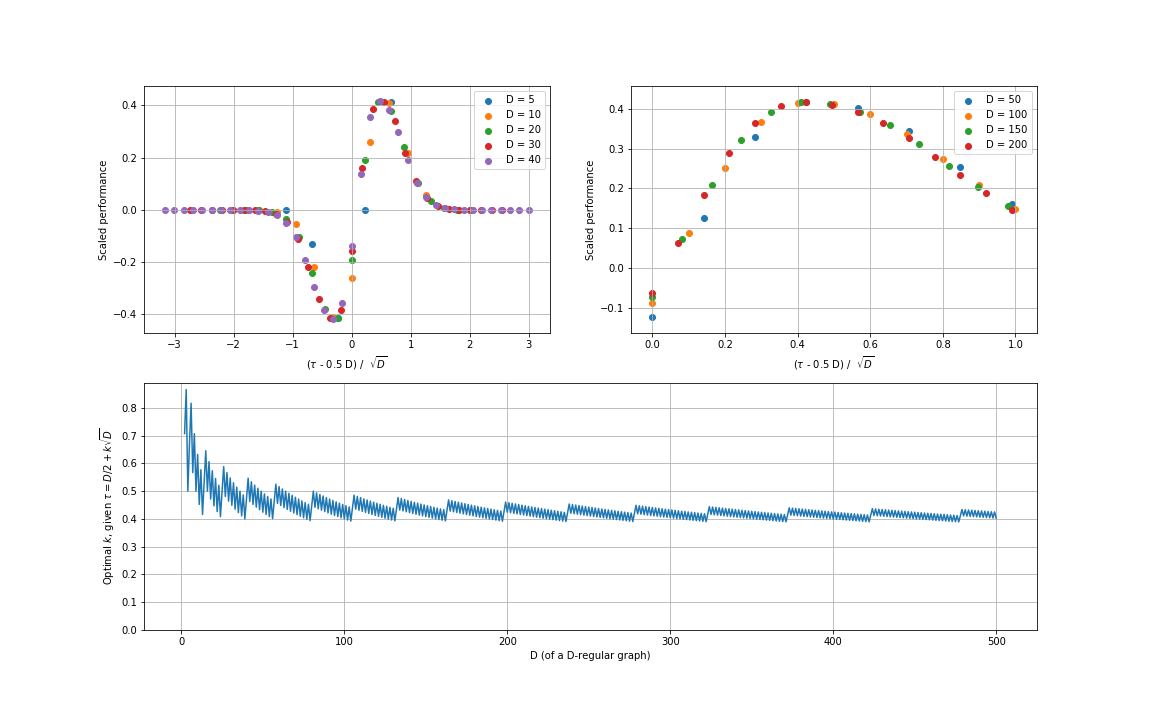
We derive an expression for the performance of the 2-step threshold algorithm on graphs of girth >5>5 as a function of τ1,τ2\tau_{1},\tau_{2}. The derivation is in Appendix D. We directly calculate the maximum value across all thresholds for small values of DD, first assuming τ1=τ2\tau_{1}=\tau_{2}. The optimal threshold approximately matches the value given in [HRSS14]: τ=D/2+kD\tau=D/2+k\sqrt{D}, where k0.4k\approx 0.4. For intermediate values of DD up to 500, we limit our search of optimal τ1,τ2\tau_{1},\tau_{2}. See Figure 1 for details.

Refer to caption
Figure 1: Top: Scaled performance of the 2-step threshold algorithm compared to threshold τ1=τ2\tau_{1}=\tau_{2}. The scaled performance is bb such that the cut fraction is 1/2+bD0.51/2+bD^{-0.5}. The left plot matches results from the 1-step threshold algorithm, as shown in Figure 6 of [HRSS14]. The right plot uses larger values of DD with a comparatively smaller region of thresholds. Note that the optimal threshold is near D/2+0.4DD/2+0.4\sqrt{D} for any DD-regular graph. This informed our search space to locate the optimal threshold at larger DD. Bottom: Optimal threshold for the 2-step threshold algorithm where τ1=τ2\tau_{1}=\tau_{2}. Notice the convergence on a value close to D/2+0.4DD/2+0.4\sqrt{D}. We use a limited search space at larger DD: within (D/2+kminDD/2+k_{min}\sqrt{D}, D/2+kmaxDD/2+k_{max}\sqrt{D}), where (kmin,kmax)=(0.3,0.6)(k_{min},k_{max})=(0.3,0.6) for 60<D15060<D\leq 150, and (kmin,kmax)=(0.35,0.52)(k_{min},k_{max})=(0.35,0.52) for D>150D>150. The optimal kk at large DD is quite close to that for the 1-step threshold algorithm, as presented in Figures 7-8 of [HRSS14].

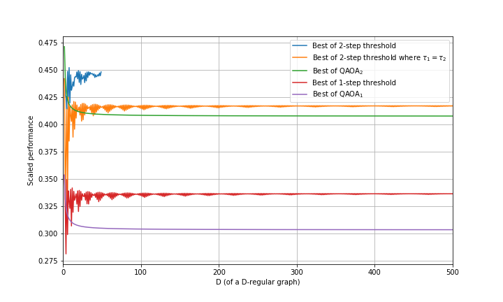
When the thresholds match, the performance of this algorithm stabilizes at 0.5+b/D0.5+b/\sqrt{D}, where b0.417b\approx 0.417. This outperforms QAOA2 for all 41<D<50041<D<500. Considering Figure 2 in a similar spirit to Figure 3 of [Has19], we expect the 2-step threshold algorithm to outperform QAOA2 for all D500D\geq 500. Note the oscillations that decrease in value for large DD, similar to those of the 1-step threshold algorithm. As [Has19] suggests, this likely happens from optimizing a discrete parameter τ\tau instead of a continuous one. We also consider thresholds where τ1\tau_{1} may not equal τ2\tau_{2} in general for all 2D<502\leq D<50; when D>5D>5, there are choices of τ1,τ2\tau_{1},\tau_{2} that outperform QAOA2. See Figure 2 for a comparison.

For D[2,3,4,5]D\in[2,3,4,5], we draw inspiration from modifications made to the 1-step threshold algorithm in Section III of [Has19]. Using the local algorithm description from [Has19], we consider a 2-step linear algorithm with entries of v0\vec{v_{0}} chosen randomly from [1,1][-1,1]. Because there are a finite number of initial values, we can exactly calculate the expected performance on a local subgraph. We search for values of (c0,c1)(c_{0},c_{1}) that outperform QAOA2. This was successful for D[3,4,5]D\in[3,4,5], but did not work for D=2D=2. In this case, we also searched over choices of initial values to find parameters that outperform QAOA2. In particular, given initial values [0.49,0.45,0.01,0.03,0.29,0.85][-0.49,-0.45,0.01,0.03,0.29,0.85], a D=2D=2 local classical algorithm has expected performance 0.33430.3343 over random assignment, whereas QAOA2 has at most 1/31/3 over random assignment [MFS19]. Many choices of initial values give a D=2D=2 classical algorithm with maximum expected performance near this value; we are unsure why this is the case.

Thus, there exists a local classical MAX-CUT algorithm that, on average, finds a larger cut than QAOA2 on every DD-regular graph of girth above 5 when D<500D<500, and likely for all DD. The expected performance values at small DD are reproduced in Appendix A. An interactive notebook [PG07] with all relevant code and figures is available online.

Refer to caption
Figure 2: Performance of approximate MAX-CUT algorithms on DD-regular graphs of girth >5>5. This plot reproduces and extends Figure 3 of [Has19]. The scaled performance bb is such that the cut fraction is 1/2+bD0.51/2+bD^{-0.5}. For QAOA2, the plot is smooth and similar in shape to QAOA1, while the 2-step threshold algorithm oscillates like the 1-step variant. At large degree, b0.417b\approx 0.417 for the 2-step threshold algorithm, which outperforms b0.407b\approx 0.407 for QAOA2, itself an improvement over both b0.33b\approx 0.33 for the 1-step threshold algorithm and b0.303b\approx 0.303 for QAOA1. Judging by the convergence at larger DD, we expect the 2-step classical algorithm to outperform QAOA2 for all D500D\geq 500.

4 Discussion

QAOAp’s optimal performance is guaranteed to increase with increasing pp. At p=2p=2, this value was previously known only in a few cases [WHJR18] [WL20]. Our approach is to directly calculate a graph-size-independent formula and optimize over parameters, which requires careful accounting of all terms. Hypothetically, Appendix B can be extended to remove the high-girth and regularity constraints. Without the regularity constraint, a graph cannot be described with a single parameter DD; without the high-girth constraint, there may be implicit combinatorial sums as in Appendix A of [WHJR18].

We wonder if QAOAp’s optimal performance on high-girth graphs is more connected to “locality” than “quantumness”. The high-girth condition makes the graph look like a tree to any local algorithm. Given any constant pp, we expect that a graph-size-independent expression can be efficiently calculated for both QAOAp and the pp-step threshold algorithm on regular graphs of girth >2p+1>2p+1; we suspect the pp-local classical algorithm, on average, will find a larger cut than QAOAp on every such graph.

Importantly, we compare QAOA2 with local classical MAX-CUT algorithms. This constraint may be useful in distributed settings, where computing nodes do not have access to the entire graph and communication between computing nodes is limited. Even so, this work suggests that QAOAp is outperformed by a local classical algorithm of similar depth. We conjecture that for every constant pp, there exists a local classical algorithm that, on average, finds a cut at least as large as QAOAp on every possible graph.

We only study DD-regular graphs. If the graph has instead maximum degree DD, one can still use this analysis by instituting “phantom vertices”, where random data is generated for each missing vertex. We first learned of this idea from [She92] but do not think it is optimal. We also compare graphs only of girth above 5. If there are a small number of short cycles, we do not expect this result to change; however, threshold algorithms are not very effective on highly connected graphs, a topic we plan to study further.

Acknowledgements

Thanks to Ryan Avery and Sangeeta Marwaha for helpful discussions. Thanks to Boaz Barak for detailed comments on the abstract and introduction. Thanks to Patrick Lutz, Bryan O’Gorman, and Akshay Ramachandran for reading a draft and providing suggestions. Thanks to Birgitta Whaley and everyone at BQIC for listening to a talk of preliminary results.

References

  • [AAB+20] F. Arute, K. Arya, R. Babbush, et al. Quantum approximate optimization of non-planar graph problems on a planar superconducting processor. 2004.04197, doi:10.1038/s41567-020-01105-y.
  • [BMO+15] B. Barak, A. Moitra, R. O’Donnell, et al. Beating the random assignment on constraint satisfaction problems of bounded degree. 1505.03424.
  • [FGG14] E. Farhi, J. Goldstone, and S. Gutmann. A quantum approximate optimization algorithm. 1411.4028.
  • [FGG15] E. Farhi, J. Goldstone, and S. Gutmann. A quantum approximate optimization algorithm applied to a bounded occurrence constraint problem. 1412.6062.
  • [GW95] M. X. Goemans and D. P. Williamson. Improved approximation algorithms for maximum cut and satisfiability problems using semidefinite programming. Journal of the ACM (JACM), 42(6):1115–1145, 1995. doi:10.1145/227683.227684, URL http://www-math.mit.edu/~goemans/PAPERS/maxcut-jacm.pdf.
  • [Has19] M. B. Hastings. Classical and quantum bounded depth approximation algorithms. 1905.07047.
  • [HRSS14] J. Hirvonen, J. Rybicki, S. Schmid, and J. Suomela. Large cuts with local algorithms on triangle-free graphs. 1402.2543.
  • [Kho02] S. Khot. On the power of unique 2-prover 1-round games. In Proceedings of the Thiry-Fourth Annual ACM Symposium on Theory of Computing, STOC ’02, page 767–775, New York, NY, USA, 2002. Association for Computing Machinery. doi:10.1145/509907.510017.
  • [MFS19] G. B. Mbeng, R. Fazio, and G. Santoro. Quantum annealing: a journey through digitalization, control, and hybrid quantum variational schemes. 1906.08948.
  • [MRBAG16] J. R. McClean, J. Romero, R. Babbush, and A. Aspuru-Guzik. The theory of variational hybrid quantum-classical algorithms. New Journal of Physics, 18(2):023023, feb 2016. doi:10.1088/1367-2630/18/2/023023.
  • [MSP+17] A. Meurer, C. P. Smith, M. Paprocki, et al. Sympy: symbolic computing in python. PeerJ Computer Science, 3:e103, Jan. 2017. doi:10.7717/peerj-cs.103.
  • [PG07] F. Pérez and B. E. Granger. IPython: a system for interactive scientific computing. Computing in Science and Engineering, 9(3):21–29, May 2007. doi:10.1109/MCSE.2007.53, URL https://ipython.org.
  • [Pre18] J. Preskill. Quantum computing in the nisq era and beyond. Quantum, 2:79, Aug 2018. doi:10.22331/q-2018-08-06-79.
  • [She92] J. B. Shearer. A note on bipartite subgraphs of triangle-free graphs. Random Structures & Algorithms, 3(2):223–226, 1992. doi:10.1002/rsa.3240030211.
  • [Sze19] M. Szegedy. What do qaoa energies reveal about graphs? 1912.12277.
  • [VGO+20] P. Virtanen, R. Gommers, T. E. Oliphant, et al. SciPy 1.0: Fundamental Algorithms for Scientific Computing in Python. Nature Methods, 17:261–272, 2020. doi:10.1038/s41592-019-0686-2.
  • [WHJR18] Z. Wang, S. Hadfield, Z. Jiang, and E. G. Rieffel. Quantum approximate optimization algorithm for maxcut: A fermionic view. Phys. Rev. A, 97:022304, Feb 2018. doi:10.1103/PhysRevA.97.022304.
  • [WL20] J. Wurtz and P. J. Love. Bounds on maxcut qaoa performance for p>>1. 2010.11209.
  • [ZWC+20] L. Zhou, S.-T. Wang, S. Choi, et al. Quantum approximate optimization algorithm: Performance, mechanism, and implementation on near-term devices. Physical Review X, 10(2), Jun 2020. doi:10.1103/physrevx.10.021067.

Appendix A Listing of performance values at small DD

D QAOA1 Threshold1 (τ\tau) Modified Threshold1 QAOA2 Threshold2 (τ1\tau_{1}, τ2\tau_{2}) Modified Threshold2 (c0c_{0}, c1c_{1})
2 0.2500 0.2500 (2) 0.3333 0.3125 (2, 2) 0.3343 (17.96, 0.56)
3 0.1925 0.1875 (3) 0.1980 0.2559 0.2461 (2, 3) 0.2703 (7.22, 0.58)
4 0.1624 0.1406 (3) 0.2161 0.1693 0.2128 (3, 4) 0.2309 (0.38, 11.20)
5 0.1431 0.1562 (4) 0.1907 0.1851 (4, 4) 0.2045 (5.44, 0.33)
6 0.1294 0.1221 (5) 0.1302 0.1726 0.1832 (4, 5)
7 0.1190 0.1282 (5) 0.1589 0.1607 (5, 5)
8 0.1108 0.1166 (6) 0.1480 0.1599 (5, 6)
9 0.1040 0.1077 (6) 0.1391 0.1399 (5, 7)
10 0.0984 0.1077 (7) 0.1317 0.1409 (6, 7)
11 0.0936 0.0925 (7) 0.0986 0.1253 0.1301 (7, 8)
12 0.0894 0.0987 (8) 0.1197 0.1254 (7, 8)
13 0.0858 0.0886 (9) 0.1149 0.1218 (8, 9)
14 0.0825 0.0905 (9) 0.1106 0.1163 (8, 10)
15 0.0796 0.0853 (10) 0.1067 0.1143 (9, 10)
16 0.0770 0.0833 (10) 0.1032 0.1110 (9, 11)
17 0.0747 0.0816 (11) 0.1001 0.1076 (10, 11)
18 0.0725 0.0771 (11) 0.0972 0.1056 (10, 12)
19 0.0705 0.0778 (12) 0.0945 0.1014 (11, 12)
Table 1: Improvement over random assignment for MAX-CUT on regular graphs of girth above 5. The degree DD is shown in the first column. “Threshold1 (τ\tau)”, “Modified Threshold1” and “QAOA1” are reproduced from Table I of [Has19]. The QAOA2 and 2-step threshold outperform all previously known values at each listed DD, and all D<500D<500 as shown numerically. “Threshold2” refers to the best 2-step threshold algorithm with τ1\tau_{1} and τ2\tau_{2} possibly unequal. It does not outperform QAOA2 when D[2,3,4,5]D\in[2,3,4,5], but a related 2-step local classical algorithm using [Has19]’s framework does.

Appendix B Proof of the p=2p=2 QAOA formula

This analysis follows the approach given in Appendix A of [WHJR18]. Assume the graph is DD-regular, and has no triangles, squares, or pentagons (girth >5>5). In addition to the variables defined in 2, let p=cos(γ1/2)p=\cos(\gamma_1 / 2), q=sin(γ1/2)q=\sin(\gamma_1 / 2), k=cos(β1)k=\cos(\beta_1), and l=sin(β1)l=\sin(\beta_1). Then, by double-angle formulas, r=k2l2r=k^{2}-l^{2}, t=2klt=2kl, y=p2q2y=p^{2}-q^{2}, and z=2pqz=2pq. We start with the expression for f2(γ1,β1,γ2,β2)f_{2}(\gamma_{1},\beta_{1},\gamma_{2},\beta_{2}), simplifying CuvC_{uv} as in Appendix A of [WHJR18]:

f2(γ1,β1,γ2,β2)=1212Tr[ρ0eiγ1Ceiβ1Jeiγ2C(c2σuzσvz+cs(σuyσvz+σuzσvy)+s2σuyσvy)eiγ2Ceiβ1Jeiγ1C]f_{2}(\gamma_{1},\beta_{1},\gamma_{2},\beta_{2})=\frac{1}{2}-\frac{1}{2}\Tr[\rho_{0}e^{i\gamma_{1}C}e^{i\beta_{1}J}e^{i\gamma_{2}C}\Big(c^{2}\sigma_{u}^{z}\sigma_{v}^{z}+cs(\sigma_{u}^{y}\sigma_{v}^{z}+\sigma_{u}^{z}\sigma_{v}^{y})+s^{2}\sigma_{u}^{y}\sigma_{v}^{y}\Big)e^{-i\gamma_{2}C}e^{-i\beta_{1}J}e^{-i\gamma_{1}C}]

We compute each of the four terms inside the trace separately, labeled so that f2=0.50.5(A+B1+B2+E)f_{2}=0.5-0.5(A+B_{1}+B_{2}+E).

B.1 Calculating AA

Since CC commutes with σuzσvz\sigma_{u}^{z}\sigma_{v}^{z}, f1=0.50.5A/c2f_{1}=0.5-0.5A/c^{2}. As the graph is DD-regular and has no triangles:

A/c2=sin(4β1)sin(γ1)cosD1(γ1)=2rtyD1zA/c^{2}=-\sin(4\beta_1)\sin(\gamma_1)\cos^{D-1}(\gamma_{1})=-2rty^{D-1}z

B.2 Calculating B1B_{1} and B2B_{2}

B.2.1 Evaluating exponentials

Since the graph is identical from uu and vv’s perspective, B1=B2B_{1}=B_{2}.

B1/cs=Tr[ρ0eiγ1Ceiβ1Jeiγ2Cσuyσvzeiγ2Ceiβ1Jeiγ1C]B_{1}/cs=\Tr[\rho_{0}e^{i\gamma_{1}C}e^{i\beta_{1}J}e^{i\gamma_{2}C}\sigma_{u}^{y}\sigma_{v}^{z}e^{-i\gamma_{2}C}e^{-i\beta_{1}J}e^{-i\gamma_{1}C}]

The only terms of CC that do not commute with σuyσvz\sigma_{u}^{y}\sigma_{v}^{z} involve nodes w1,wD1,vw_{1},...w_{D-1},v adjacent to uu.

B1/cs=Tr[ρ0eiγ1Ceiβ1J(i=1D1eiγ2σuzσwiz)eiγ2σuzσvzσuyσvzeiβ1Jeiγ1C]B_{1}/cs=\Tr[\rho_{0}e^{i\gamma_{1}C}e^{i\beta_{1}J}\big(\prod_{i=1}^{D-1}e^{-i\gamma_{2}\sigma_{u}^{z}\sigma_{w_{i}}^{z}}\big)e^{-i\gamma_{2}\sigma_{u}^{z}\sigma_{v}^{z}}\sigma_{u}^{y}\sigma_{v}^{z}e^{-i\beta_{1}J}e^{-i\gamma_{1}C}]

The only terms of JJ that do not commute with the inner expression reference the nodes u,v,w1,,wD1u,v,w_{1},...,w_{D-1}.

B1/cs=Tr[ρ0eiγ1Ceiβ1σux(i=1D1eiβ1σwixeiγ2σuzσwizeiβ1σwix)(eiβ1σvxeiγ2σuzσvzeiβ1σvx)eiβ1σuxσuyσvzeiγ1C]B_{1}/cs=\Tr[\rho_{0}e^{i\gamma_{1}C}e^{i\beta_{1}\sigma_{u}^{x}}\big(\prod_{i=1}^{D-1}e^{i\beta_{1}\sigma_{w_{i}}^{x}}e^{-i\gamma_{2}\sigma_{u}^{z}\sigma_{w_{i}}^{z}}e^{-i\beta_{1}\sigma_{w_{i}}^{x}}\big)\big(e^{i\beta_{1}\sigma_{v}^{x}}e^{-i\gamma_{2}\sigma_{u}^{z}\sigma_{v}^{z}}e^{i\beta_{1}\sigma_{v}^{x}}\big)e^{i\beta_{1}\sigma_{u}^{x}}\sigma_{u}^{y}\sigma_{v}^{z}e^{-i\gamma_{1}C}]

The terms in parentheses can be simplified.

eiβ1σwixeiγ2σuzσwizeiβ1σwix=eiβ1σwix(minσuzσwiz)eiβ1σwix=mine2iβ1σwixσuzσwize^{i\beta_{1}\sigma_{w_{i}}^{x}}e^{-i\gamma_{2}\sigma_{u}^{z}\sigma_{w_{i}}^{z}}e^{-i\beta_{1}\sigma_{w_{i}}^{x}}=e^{i\beta_{1}\sigma_{w_{i}}^{x}}(m-in\sigma_{u}^{z}\sigma_{w_{i}}^{z})e^{-i\beta_{1}\sigma_{w_{i}}^{x}}=m-ine^{2i\beta_{1}\sigma_{w_{i}}^{x}}\sigma_{u}^{z}\sigma_{w_{i}}^{z}
eiβ1σvxeiγ2σuzσvzeiβ1σvx=eiβ1σvx(minσuzσvz)eiβ1σvx=e2iβ1σvxminσuzσvze^{i\beta_{1}\sigma_{v}^{x}}e^{-i\gamma_{2}\sigma_{u}^{z}\sigma_{v}^{z}}e^{i\beta_{1}\sigma_{v}^{x}}=e^{i\beta_{1}\sigma_{v}^{x}}(m-in\sigma_{u}^{z}\sigma_{v}^{z})e^{i\beta_{1}\sigma_{v}^{x}}=e^{2i\beta_{1}\sigma_{v}^{x}}m-in\sigma_{u}^{z}\sigma_{v}^{z}
B1/cs=Tr[ρ0eiγ1Ceiβ1σux(i=1D1mine2iβ1σwixσuzσwiz)(e2iβ1σvxminσuzσvz)eiβ1σuxσuyσvzeiγ1C]B_{1}/cs=\Tr[\rho_{0}e^{i\gamma_{1}C}e^{i\beta_{1}\sigma_{u}^{x}}\big(\prod_{i=1}^{D-1}m-ine^{2i\beta_{1}\sigma_{w_{i}}^{x}}\sigma_{u}^{z}\sigma_{w_{i}}^{z}\big)\big(e^{2i\beta_{1}\sigma_{v}^{x}}m-in\sigma_{u}^{z}\sigma_{v}^{z}\big)e^{i\beta_{1}\sigma_{u}^{x}}\sigma_{u}^{y}\sigma_{v}^{z}e^{-i\gamma_{1}C}]

B.2.2 Breaking apart into terms

The only terms of CC that may not commute involve edges connected to a node in S={u,v,w1,,wD1}S=\{u,v,w_{1},...,w_{D-1}\}. Terms of eiγ1Ce^{i\gamma_{1}C} that connect jj and kk have the form piqσjzσkzp-iq\sigma_{j}^{z}\sigma_{k}^{z}. Consider edges where both j,kSj,k\in S; we discuss the other edges in Appendix B.2.3.

B1/cs=Tr[ρ0(piqσuzσvz)(i=1D1(piqσuzσwiz))eiβ1σux(i=1D1(mine2iβ1σwixσuzσwiz))(e2iβ1σvxminσuzσvz)eiβ1σux(piqσuzσvz)(i=1D1(piqσuzσwiz))σuyσvz]B_{1}/cs=\text{Tr}\Bigg[\rho_{0}(p-iq\sigma_{u}^{z}\sigma_{v}^{z})\big(\prod_{i=1}^{D-1}(p-iq\sigma_{u}^{z}\sigma_{w_{i}}^{z})\big)\\ e^{i\beta_{1}\sigma_{u}^{x}}\big(\prod_{i=1}^{D-1}(m-ine^{2i\beta_{1}\sigma_{w_{i}}^{x}}\sigma_{u}^{z}\sigma_{w_{i}}^{z})\big)\big(e^{2i\beta_{1}\sigma_{v}^{x}}m-in\sigma_{u}^{z}\sigma_{v}^{z}\big)e^{i\beta_{1}\sigma_{u}^{x}}\\ (p-iq\sigma_{u}^{z}\sigma_{v}^{z})\big(\prod_{i=1}^{D-1}(p-iq\sigma_{u}^{z}\sigma_{w_{i}}^{z})\big)\sigma_{u}^{y}\sigma_{v}^{z}\Bigg]

We will expand the products carefully. Many terms do not contribute to trace. Only half include an even number of σvz\sigma_{v}^{z}; the rest will not contribute to trace because of the definition of ρ0\rho_{0}. Note that each of these terms includes an odd number of σuz\sigma_{u}^{z}, correctly cancelling out the rightmost σuy\sigma_{u}^{y} in the trace. Consider the terms that include σvz\sigma_{v}^{z}:

(piqσuzσvz)(e2iβ1σvxminσuzσvz)(piqσuzσvz)σvz(p-iq\sigma_{u}^{z}\sigma_{v}^{z})\cdots(e^{2i\beta_{1}\sigma_{v}^{x}}m-in\sigma_{u}^{z}\sigma_{v}^{z})\cdots(p-iq\sigma_{u}^{z}\sigma_{v}^{z})\sigma_{v}^{z}
  1. 1.

    (iqσuzσvz,e2iβ1σvxm,pσvz)V1=impqe2iβ1σvx(-iq\sigma_{u}^{z}\sigma_{v}^{z},e^{2i\beta_{1}\sigma_{v}^{x}}m,p\sigma_{v}^{z})\to V_{1}=-impqe^{-2i\beta_{1}\sigma_{v}^{x}}

  2. 2.

    (p,inσuzσvz,pσvz)V2=inp2(p,-in\sigma_{u}^{z}\sigma_{v}^{z},p\sigma_{v}^{z})\to V_{2}=-inp^{2}

  3. 3.

    (p,e2iβ1σvxm,iqσuzσvzσvz)V3=impqe2iβ1σvx(p,e^{2i\beta_{1}\sigma_{v}^{x}}m,-iq\sigma_{u}^{z}\sigma_{v}^{z}\sigma_{v}^{z})\to V_{3}=-impqe^{2i\beta_{1}\sigma_{v}^{x}}

  4. 4.

    (iqσuzσvz,inσuzσvz,iqσuzσvzσvz)V4=inq2(-iq\sigma_{u}^{z}\sigma_{v}^{z},-in\sigma_{u}^{z}\sigma_{v}^{z},-iq\sigma_{u}^{z}\sigma_{v}^{z}\sigma_{v}^{z})\to V_{4}=inq^{2}

Similarly, of the expressions that include σwiz\sigma_{w_{i}}^{z}, only half include an even number. Only these corresponding terms can contribute to trace. Note that each of these terms includes an even number of σuz\sigma_{u}^{z}, which will cancel out. Sometimes the exponential sign flips when commuting with σz\sigma^{z}.

(piqσuzσwiz)(mine2iβ1σwixσuzσwiz)(piqσuzσwiz)(p-iq\sigma_{u}^{z}\sigma_{w_{i}}^{z})\cdots(m-ine^{2i\beta_{1}\sigma_{w_{i}}^{x}}\sigma_{u}^{z}\sigma_{w_{i}}^{z})\cdots(p-iq\sigma_{u}^{z}\sigma_{w_{i}}^{z})
  1. 1.

    (p,m,p)W1=mp2(p,m,p)\to W_{1}=mp^{2}

  2. 2.

    (p,ine2iβ1σwixσuzσwiz,iqσuzσwiz)W2=npqe2iβ1σwix(p,-ine^{2i\beta_{1}\sigma_{w_{i}}^{x}}\sigma_{u}^{z}\sigma_{w_{i}}^{z},-iq\sigma_{u}^{z}\sigma_{w_{i}}^{z})\to W_{2}=-npqe^{2i\beta_{1}\sigma_{w_{i}}^{x}}

  3. 3.

    (iqσuzσwiz,m,iqσuzσwiz)W3=mq2(-iq\sigma_{u}^{z}\sigma_{w_{i}}^{z},m,-iq\sigma_{u}^{z}\sigma_{w_{i}}^{z})\to W_{3}=-mq^{2}

  4. 4.

    (iqσuzσwiz,ine2iβ1σwixσuzσwiz,p)W4=npqe2iβ1σwix(-iq\sigma_{u}^{z}\sigma_{w_{i}}^{z},-ine^{2i\beta_{1}\sigma_{w_{i}}^{x}}\sigma_{u}^{z}\sigma_{w_{i}}^{z},p)\to W_{4}=-npqe^{-2i\beta_{1}\sigma_{w_{i}}^{x}}

The last step is to consider the expression eiβ1σux=k+ilσuxe^{i\beta_{1}\sigma_{u}^{x}}=k+il\sigma_{u}^{x}. Each combination of terms is matched with its contribution to trace. If the first expression eiβ1σuxe^{i\beta_{1}\sigma_{u}^{x}} includes ilσuxil\sigma_{u}^{x}, it will flip the sign of V1,V4,W3,W4V_{1},V_{4},W_{3},W_{4}. If the second expression eiβ1σuxe^{i\beta_{1}\sigma_{u}^{x}} includes ilσuxil\sigma_{u}^{x}, it will flip the sign of V1,V2,W2,W3V_{1},V_{2},W_{2},W_{3}.

  1. 1.

    (k,k)Tr[(k)(k)(V1+V2+V3+V4)(W1+W2+W3+W4)D1σuzσuy](k,k)\to\Tr[(k)(k)(V_{1}+V_{2}+V_{3}+V_{4})(W_{1}+W_{2}+W_{3}+W_{4})^{D-1}\sigma_{u}^{z}\sigma_{u}^{y}]

  2. 2.

    (k,l)Tr[(k)(il)(V1V2+V3+V4)(W1W2W3+W4)D1σuzσuy](k,l)\to\Tr[(k)(il)(-V_{1}-V_{2}+V_{3}+V_{4})(W_{1}-W_{2}-W_{3}+W_{4})^{D-1}\sigma_{u}^{z}\sigma_{u}^{y}]

  3. 3.

    (l,k)Tr[(il)(k)(V1+V2+V3V4)(W1+W2W3W4)D1σuzσuy](l,k)\to\Tr[(il)(k)(-V_{1}+V_{2}+V_{3}-V_{4})(W_{1}+W_{2}-W_{3}-W_{4})^{D-1}\sigma_{u}^{z}\sigma_{u}^{y}]

  4. 4.

    (l,l)Tr[(il)(il)(V1V2+V3V4)(W1W2+W3W4)D1σuzσuy](l,l)\to\Tr[(il)(il)(V_{1}-V_{2}+V_{3}-V_{4})(W_{1}-W_{2}+W_{3}-W_{4})^{D-1}\sigma_{u}^{z}\sigma_{u}^{y}]

The VV and WW sums can then be simplified. Any expressions using eiaσxe^{ia\sigma^{x}} will become eiae^{ia} after taking the trace. Here are the VV sums:

V1+V2+V3+V4\displaystyle V_{1}+V_{2}+V_{3}+V_{4} =impqe2iβ1+inp2+impqe2iβ1+inq2=impq(2r)in(p2q2)=imrziny\displaystyle=-impqe^{-2i\beta_{1}}+-inp^{2}+-impqe^{2i\beta_{1}}+inq^{2}=-impq(2r)-in(p^{2}-q^{2})=-imrz-iny
V1V2+V3+V4\displaystyle-V_{1}-V_{2}+V_{3}+V_{4} =impqe2iβ1inp2+impqe2iβ1+inq2=impq(2it)+in(p2+q2)=mtz+in\displaystyle=--impqe^{-2i\beta_{1}}--inp^{2}+-impqe^{2i\beta_{1}}+inq^{2}=-impq(2it)+in(p^{2}+q^{2})=mtz+in
V1+V2+V3V4\displaystyle-V_{1}+V_{2}+V_{3}-V_{4} =impqe2iβ1+inp2+impqe2iβ1inq2=impq(2it)in(p2+q2)=mtzin\displaystyle=--impqe^{-2i\beta_{1}}+-inp^{2}+-impqe^{2i\beta_{1}}-inq^{2}=-impq(2it)-in(p^{2}+q^{2})=mtz-in
V1V2+V3V4\displaystyle V_{1}-V_{2}+V_{3}-V_{4} =impqe2iβ1inp2+impqe2iβ1inq2=impq(2r)+in(p2q2)=imrz+iny\displaystyle=-impqe^{-2i\beta_{1}}--inp^{2}+-impqe^{2i\beta_{1}}-inq^{2}=-impq(2r)+in(p^{2}-q^{2})=-imrz+iny

Here are the WW sums:

W1+W2+W3+W4\displaystyle W_{1}+W_{2}+W_{3}+W_{4} =mp2+npqe2iβ1+mq2+npqe2iβ1\displaystyle=mp^{2}+-npqe^{2i\beta_{1}}+-mq^{2}+-npqe^{-2i\beta_{1}} =m(p2q2)npq(2r)\displaystyle=m(p^{2}-q^{2})-npq(2r) =mynrz\displaystyle=my-nrz
W1W2W3+W4\displaystyle W_{1}-W_{2}-W_{3}+W_{4} =mp2npqe2iβ1mq2+npqe2iβ1\displaystyle=mp^{2}--npqe^{2i\beta_{1}}--mq^{2}+-npqe^{-2i\beta_{1}} =m(p2+q2)+npq(2it)\displaystyle=m(p^{2}+q^{2})+npq(2it) =m+intz\displaystyle=m+intz
W1+W2W3W4\displaystyle W_{1}+W_{2}-W_{3}-W_{4} =mp2+npqe2iβ1mq2npqe2iβ1\displaystyle=mp^{2}+-npqe^{2i\beta_{1}}--mq^{2}--npqe^{-2i\beta_{1}} =m(p2+q2)npq(2it)\displaystyle=m(p^{2}+q^{2})-npq(2it) =mintz\displaystyle=m-intz
W1W2+W3W4\displaystyle W_{1}-W_{2}+W_{3}-W_{4} =mp2npqe2iβ1+mq2npqe2iβ1\displaystyle=mp^{2}--npqe^{2i\beta_{1}}+-mq^{2}--npqe^{-2i\beta_{1}} =m(p2q2)+npq(2r)\displaystyle=m(p^{2}-q^{2})+npq(2r) =my+nrz\displaystyle=my+nrz

We sum all terms. Notice that any ViWjV_{i}W_{j} will include an odd number of σuz\sigma_{u}^{z}, which combined with σuy\sigma_{u}^{y} will add a factor of i-i to each term in the trace:

B1/cs=(i)(k2(imrziny)(mynrz)D1+ikl(mtz+in)(m+intz)D1CLOSEOPEN+ikl(mtzin)(mintz)D1l2(imrz+iny)(my+nrz)D1)B_{1}/cs=(-i)\Big(k^{2}(-imrz-iny)(my-nrz)^{D-1}+ikl(mtz+in)(m+intz)^{D-1}\\ +ikl(mtz-in)(m-intz)^{D-1}-l^{2}(-imrz+iny)(my+nrz)^{D-1}\Big)

In a simplified form,

B1/cs=0.5((1+r)(mrzny)(mynrz)D1+t(mtz+in)(m+intz)D1CLOSEOPEN+t(mtzin)(mintz)D1+(1r)(mrzny)(my+nrz)D1)B_{1}/cs=0.5\Big((1+r)(-mrz-ny)(my-nrz)^{D-1}+t(mtz+in)(m+intz)^{D-1}\\ +t(mtz-in)(m-intz)^{D-1}+(1-r)(mrz-ny)(my+nrz)^{D-1}\Big)

B.2.3 Effect of the crossover terms

Now we consider the crossover terms. For edges that introduced a new node kk, the associated σzk\sigma_{z}^{k} must be cancelled. Since the graph has girth above 5, any neighbor kSk\notin S to S\ell\in S has a unique neighbor \ell. So, the above expression is modified by

Tr[(piqσjzσkz)(p+iqσjzσkz)]=p2Tr[]+q2[σjzσjz]\Tr[(p-iq\sigma_{j}^{z}\sigma_{k}^{z})\cdots(p+iq\sigma_{j}^{z}\sigma_{k}^{z})]=p^{2}\Tr[\cdots]+q^{2}[\sigma_{j}^{z}\cdots\sigma_{j}^{z}]

For =v\ell=v, the only term that does not commute with σvz\sigma_{v}^{z} is e2iβ1σvxme2iβ1σvxme^{2i\beta_{1}\sigma_{v}^{x}}m\to e^{-2i\beta_{1}\sigma_{v}^{x}}m. This swaps V1V_{1} and V3V_{3}, which only adjusts mtzmtzmtz\to-mtz in the 2nd and 3rd term of the above expression. Thus, mtz(p2q2)mtz=mtyzmtz\to(p^{2}-q^{2})mtz=mtyz. All other terms are T(p2+q2)T=TT\to(p^{2}+q^{2})T=T. This process happens D1D-1 times (once for each neighbor xjux_{j}\neq u of vv).

B1/cs=0.5((1+r)(mrzny)(mynrz)D1+t(mtyD1z+in)(m+intz)D1+CLOSEOPENt(mtyD1zin)(mintz)D1+(1r)(mrzny)(my+nrz)D1)B_{1}/cs=0.5\Big((1+r)(-mrz-ny)(my-nrz)^{D-1}+t(mty^{D-1}z+in)(m+intz)^{D-1}+\\ t(mty^{D-1}z-in)(m-intz)^{D-1}+(1-r)(mrz-ny)(my+nrz)^{D-1}\Big)

Consider =wi\ell=w_{i} for i{1,,D1}i\in\{1,\cdots,D-1\}. The only term that does not commute with σwiz\sigma_{w_{i}}^{z} is e2iβ1σwixe2iβ1σwixe^{2i\beta_{1}\sigma_{w_{i}}^{x}}\to e^{-2i\beta_{1}\sigma_{w_{i}}^{x}}. This swaps W2W_{2} and W4W_{4}, which converts (m±intz)(m\pm intz) to (mintz)(m\mp intz). Thus, (m±intz)(p2(m±intz)+q2(mintz)=(m±intyz)CLOSE(m\pm intz)\to(p^{2}(m\pm intz)+q^{2}(m\mp intz)=(m\pm intyz). All other terms are T(p2+q2)T=TT\to(p^{2}+q^{2})T=T. This process happens D1D-1 times (once for each neighbor xjux_{j}\neq u of wiw_{i}). There are D1D-1 nodes of the form wiw_{i}.

B1/cs\displaystyle B_{1}/cs =0.5((1+r)(mrzny)(mynrz)D1+t(mtyD1z+in)(m+intyD1z)D1CLOSE\displaystyle=0.5\big((1+r)(-mrz-ny)(my-nrz)^{D-1}+t(mty^{D-1}z+in)(m+inty^{D-1}z)^{D-1}
OPEN+t(mtyD1zin)(mintyD1z)D1+(1r)(mrzny)(my+nrz)D1)\displaystyle+t(mty^{D-1}z-in)(m-inty^{D-1}z)^{D-1}+(1-r)(mrz-ny)(my+nrz)^{D-1}\big)
:=0.5α(γ1,β1,γ2)\displaystyle:=0.5\alpha(\gamma_{1},\beta_{1},\gamma_{2})

B.3 Calculating EE

B.3.1 Evaluating exponentials

Most terms of CC commute with σuyσvy\sigma_{u}^{y}\sigma_{v}^{y}. The ones that do not correspond to the other D1D-1 neighbors of uu and vv.

E/s2=Tr[ρ0eiγ1Ceiβ1J(i=1D1eiγ2σuzσwiz)(j=1D1eiγ2σvzσχjz)σuyσvyeiβ1Jeiγ1C]E/s^{2}=\Tr[\rho_{0}e^{i\gamma_{1}C}e^{i\beta_{1}J}\big(\prod_{i=1}^{D-1}e^{-i\gamma_{2}\sigma_{u}^{z}\sigma_{w_{i}}^{z}}\big)\big(\prod_{j=1}^{D-1}e^{-i\gamma_{2}\sigma_{v}^{z}\sigma_{\chi_{j}}^{z}}\big)\sigma_{u}^{y}\sigma_{v}^{y}e^{-i\beta_{1}J}e^{-i\gamma_{1}C}]

The only terms of JJ that do not commute with the inner expression involve u,v,w1,,wD1,χ1,,χD1u,v,w_{1},...,w_{D-1},\chi_{1},...,\chi_{D-1}.

E/s2=Tr[ρ0eiγ1Ceiβ1σuxeiβ1σvx(i=1D1eiβ1σwixeiγ2σuzσwizeiβ1σwix)(j=1D1eiβ1σχjxeiγ2σvzσχjzeiβ1σχjx)eiβ1σuxeiβ1σvxσuyσvyeiγ1C]E/s^{2}=\text{Tr}\Bigg[\rho_{0}e^{i\gamma_{1}C}e^{i\beta_{1}\sigma_{u}^{x}}e^{i\beta_{1}\sigma_{v}^{x}}\big(\prod_{i=1}^{D-1}e^{i\beta_{1}\sigma_{w_{i}}^{x}}e^{-i\gamma_{2}\sigma_{u}^{z}\sigma_{w_{i}}^{z}}e^{-i\beta_{1}\sigma_{w_{i}}^{x}}\big)\\ \big(\prod_{j=1}^{D-1}e^{i\beta_{1}\sigma_{\chi_{j}}^{x}}e^{-i\gamma_{2}\sigma_{v}^{z}\sigma_{\chi_{j}}^{z}}e^{-i\beta_{1}\sigma_{\chi_{j}}^{x}}\big)e^{i\beta_{1}\sigma_{u}^{x}}e^{i\beta_{1}\sigma_{v}^{x}}\sigma_{u}^{y}\sigma_{v}^{y}e^{-i\gamma_{1}C}\Bigg]

The terms within the parentheses can be simplified.

eiβ1σwixeiγ2σuzσwizeiβ1σwix=eiβ1σwix(minσuzσwiz)eiβ1σwix=mine2iβ1σwixσuzσwize^{i\beta_{1}\sigma_{w_{i}}^{x}}e^{-i\gamma_{2}\sigma_{u}^{z}\sigma_{w_{i}}^{z}}e^{-i\beta_{1}\sigma_{w_{i}}^{x}}=e^{i\beta_{1}\sigma_{w_{i}}^{x}}(m-in\sigma_{u}^{z}\sigma_{w_{i}}^{z})e^{-i\beta_{1}\sigma_{w_{i}}^{x}}=m-ine^{2i\beta_{1}\sigma_{w_{i}}^{x}}\sigma_{u}^{z}\sigma_{w_{i}}^{z}
E/s2=Tr[ρ0eiγ1Ceiβ1σuxeiβ1σvx(i=1D1mine2iβ1σwixσuzσwiz)(j=1D1mine2iβ1σχjxσvzσχjz)eiβ1σuxeiβ1σvxσuyσvyeiγ1C]E/s^{2}=\Tr[\rho_{0}e^{i\gamma_{1}C}e^{i\beta_{1}\sigma_{u}^{x}}e^{i\beta_{1}\sigma_{v}^{x}}\big(\prod_{i=1}^{D-1}m-ine^{2i\beta_{1}\sigma_{w_{i}}^{x}}\sigma_{u}^{z}\sigma_{w_{i}}^{z}\big)\big(\prod_{j=1}^{D-1}m-ine^{2i\beta_{1}\sigma_{\chi_{j}}^{x}}\sigma_{v}^{z}\sigma_{\chi_{j}}^{z}\big)e^{i\beta_{1}\sigma_{u}^{x}}e^{i\beta_{1}\sigma_{v}^{x}}\sigma_{u}^{y}\sigma_{v}^{y}e^{-i\gamma_{1}C}]

B.3.2 Breaking apart into terms

Terms of eiγ1Ce^{i\gamma_{1}C} that connect jj and kk have the form piqσjzσkzp-iq\sigma_{j}^{z}\sigma_{k}^{z}. If a term of CC does not commute, it must involve an edge connected to a node in R={u,v,w1,,wD1,χ1,,χD1}R=\{u,v,w_{1},...,w_{D-1},\chi_{1},...,\chi_{D-1}\}. For now, consider only edges where j,kRj,k\in R. We consider the “crossover terms” in Appendix B.3.3. Because of ρ0\rho_{0}, the trace is nonzero only for terms that are proportional to II or σnx\sigma_{n}^{x} for all nodes nn.

E/s2=Tr[ρ0(piqσuzσvz)(i=1D1(piqσuzσwiz))(j=1D1(piqσvzσχjz))eiβ1σuxeiβ1σvx(i=1D1mine2iβ1σwixσuzσwiz)(j=1D1mine2iβ1σχjxσvzσχjz)eiβ1σuxeiβ1σvx(p+iqσuzσvz)(i=1D1(piqσuzσwiz))(j=1D1(piqσvzσχjz))σuyσvy]E/s^{2}=\text{Tr}\Bigg[\rho_{0}(p-iq\sigma_{u}^{z}\sigma_{v}^{z})\big(\prod_{i=1}^{D-1}(p-iq\sigma_{u}^{z}\sigma_{w_{i}}^{z})\big)\big(\prod_{j=1}^{D-1}(p-iq\sigma_{v}^{z}\sigma_{\chi_{j}}^{z})\big)\\ e^{i\beta_{1}\sigma_{u}^{x}}e^{i\beta_{1}\sigma_{v}^{x}}\big(\prod_{i=1}^{D-1}m-ine^{2i\beta_{1}\sigma_{w_{i}}^{x}}\sigma_{u}^{z}\sigma_{w_{i}}^{z}\big)\big(\prod_{j=1}^{D-1}m-ine^{2i\beta_{1}\sigma_{\chi_{j}}^{x}}\sigma_{v}^{z}\sigma_{\chi_{j}}^{z}\big)e^{i\beta_{1}\sigma_{u}^{x}}e^{i\beta_{1}\sigma_{v}^{x}}\\ (p+iq\sigma_{u}^{z}\sigma_{v}^{z})\big(\prod_{i=1}^{D-1}(p-iq\sigma_{u}^{z}\sigma_{w_{i}}^{z})\big)\big(\prod_{j=1}^{D-1}(p-iq\sigma_{v}^{z}\sigma_{\chi_{j}}^{z})\big)\sigma_{u}^{y}\sigma_{v}^{y}\Bigg]

Any nonzero trace terms including σz\sigma_{z} or σy\sigma_{y} must be converted to II or σx\sigma_{x}. Of the expressions that include σwiz\sigma_{w_{i}}^{z}, only half include an even number. Only these corresponding terms will contribute to trace. Note that each of these terms includes an even number of σuz\sigma_{u}^{z} which cancel. Sometimes the exponential sign flips when commuting with σz\sigma^{z}. This entire process also holds for σχjz\sigma_{\chi_{j}}^{z}; let’s call those terms X1,X2,X3,X4X_{1},X_{2},X_{3},X_{4}.

(piqσuzσwiz)(mine2iβ1σwixσuzσwiz)(piqσuzσwiz)(p-iq\sigma_{u}^{z}\sigma_{w_{i}}^{z})\cdots(m-ine^{2i\beta_{1}\sigma_{w_{i}}^{x}}\sigma_{u}^{z}\sigma_{w_{i}}^{z})\cdots(p-iq\sigma_{u}^{z}\sigma_{w_{i}}^{z})
  1. 1.

    (p,m,p)W1=mp2(p,m,p)\to W_{1}=mp^{2}

  2. 2.

    (p,ine2iβ1σwixσuzσwiz,iqσuzσwiz)W2=npqe2iβ1σwix(p,-ine^{2i\beta_{1}\sigma_{w_{i}}^{x}}\sigma_{u}^{z}\sigma_{w_{i}}^{z},-iq\sigma_{u}^{z}\sigma_{w_{i}}^{z})\to W_{2}=-npqe^{2i\beta_{1}\sigma_{w_{i}}^{x}}

  3. 3.

    (iqσuzσwiz,m,iqσuzσwiz)W3=mq2(-iq\sigma_{u}^{z}\sigma_{w_{i}}^{z},m,-iq\sigma_{u}^{z}\sigma_{w_{i}}^{z})\to W_{3}=-mq^{2}

  4. 4.

    (iqσuzσwiz,ine2iβ1σwixσuzσwiz,p)W4=npqe2iβ1σwix(-iq\sigma_{u}^{z}\sigma_{w_{i}}^{z},-ine^{2i\beta_{1}\sigma_{w_{i}}^{x}}\sigma_{u}^{z}\sigma_{w_{i}}^{z},p)\to W_{4}=-npqe^{-2i\beta_{1}\sigma_{w_{i}}^{x}}

Consider the σuyσvy\sigma_{u}^{y}\sigma_{v}^{y} term. This can only be cancelled with (p±iqσuzσvz)(p\pm iq\sigma_{u}^{z}\sigma_{v}^{z}), since other terms include additional σwiz\sigma_{w_{i}}^{z} or σχjz\sigma_{\chi_{j}}^{z} which cannot be cancelled out alone. These are the only allowed terms from (piqσuzσvz)(p+iqσuzσvz)σuyσvy(p-iq\sigma_{u}^{z}\sigma_{v}^{z})\cdots(p+iq\sigma_{u}^{z}\sigma_{v}^{z})\sigma_{u}^{y}\sigma_{v}^{y}:

  1. 1.

    (p)(iqσuzσvz)σuyσvyipq(p)\cdots(iq\sigma_{u}^{z}\sigma_{v}^{z})\sigma_{u}^{y}\sigma_{v}^{y}\to-ipq

  2. 2.

    (iqσuzσvz)(p)σuyσvyipq(-iq\sigma_{u}^{z}\sigma_{v}^{z})\cdots(p)\sigma_{u}^{y}\sigma_{v}^{y}\to ipq, where all eiβ1σuxeiβ1σvxeiβ1σuxeiβ1σvxe^{i\beta_{1}\sigma_{u}^{x}}e^{i\beta_{1}\sigma_{v}^{x}}\to e^{-i\beta_{1}\sigma_{u}^{x}}e^{-i\beta_{1}\sigma_{v}^{x}}

Expanding the mentioned exponentials and summing the two terms simplifies to

2pqkl(k2l2σuxσvx)(σux+σvx)2pqkl(k^{2}-l^{2}\sigma_{u}^{x}\sigma_{v}^{x})\cdots(\sigma_{u}^{x}+\sigma_{v}^{x})

plus the terms reversed:

2pqkl(σux+σvx)(k2l2σuxσvx)2pqkl(\sigma_{u}^{x}+\sigma_{v}^{x})\cdots(k^{2}-l^{2}\sigma_{u}^{x}\sigma_{v}^{x})

Each combination of terms is matched with its contribution to trace. Note that if the first expression includes σux\sigma_{u}^{x}, it will flip the sign of W3,W4W_{3},W_{4}. If the second expression includes σux\sigma_{u}^{x}, it will flip the sign of W2,W3W_{2},W_{3}. The same is true for σvx\sigma_{v}^{x} and XX terms.

  1. 1.

    (k2,σux)Tr[2pqkl(k2)(W1W2W3+W4)D1(X1+X2+X3+X4)D1](k^{2},\sigma_{u}^{x})\to\Tr[2pqkl(k^{2})(W_{1}-W_{2}-W_{3}+W_{4})^{D-1}(X_{1}+X_{2}+X_{3}+X_{4})^{D-1}]

  2. 2.

    (k2,σvx)Tr[2pqkl(k2)(W1+W2+W3+W4)D1(X1X2X3+X4)D1](k^{2},\sigma_{v}^{x})\to\Tr[2pqkl(k^{2})(W_{1}+W_{2}+W_{3}+W_{4})^{D-1}(X_{1}-X_{2}-X_{3}+X_{4})^{D-1}]

  3. 3.

    (σux,k2)Tr[2pqkl(k2)(W1+W2W3W4)D1(X1+X2+X3+X4)D1](\sigma_{u}^{x},k^{2})\to\Tr[2pqkl(k^{2})(W_{1}+W_{2}-W_{3}-W_{4})^{D-1}(X_{1}+X_{2}+X_{3}+X_{4})^{D-1}]

  4. 4.

    (σvx,k2)Tr[2pqkl(k2)(W1+W2+W3+W4)D1(X1+X2X3X4)D1](\sigma_{v}^{x},k^{2})\to\Tr[2pqkl(k^{2})(W_{1}+W_{2}+W_{3}+W_{4})^{D-1}(X_{1}+X_{2}-X_{3}-X_{4})^{D-1}]

  5. 5.

    (l2σuxσvx,σux)Tr[2pqkl(l2)(W1W2+W3W4)D1(X1+X2X3X4)D1](-l^{2}\sigma_{u}^{x}\sigma_{v}^{x},\sigma_{u}^{x})\to\Tr[2pqkl(-l^{2})(W_{1}-W_{2}+W_{3}-W_{4})^{D-1}(X_{1}+X_{2}-X_{3}-X_{4})^{D-1}]

  6. 6.

    (l2σuxσvx,σvx)Tr[2pqkl(l2)(W1+W2W3W4)D1(X1X2+X3X4)D1](-l^{2}\sigma_{u}^{x}\sigma_{v}^{x},\sigma_{v}^{x})\to\Tr[2pqkl(-l^{2})(W_{1}+W_{2}-W_{3}-W_{4})^{D-1}(X_{1}-X_{2}+X_{3}-X_{4})^{D-1}]

  7. 7.

    (σux,l2σuxσvx)Tr[2pqkl(l2)(W1W2+W3W4)D1(X1X2X3+X4)D1](\sigma_{u}^{x},-l^{2}\sigma_{u}^{x}\sigma_{v}^{x})\to\Tr[2pqkl(-l^{2})(W_{1}-W_{2}+W_{3}-W_{4})^{D-1}(X_{1}-X_{2}-X_{3}+X_{4})^{D-1}]

  8. 8.

    (σvx,l2σuxσvx)Tr[2pqkl(l2)(W1W2W3+W4)D1(X1X2+X3X4)D1](\sigma_{v}^{x},-l^{2}\sigma_{u}^{x}\sigma_{v}^{x})\to\Tr[2pqkl(-l^{2})(W_{1}-W_{2}-W_{3}+W_{4})^{D-1}(X_{1}-X_{2}+X_{3}-X_{4})^{D-1}]

After taking the trace, each of W=XW_{\ell}=X_{\ell}. Summing all 8 combinations:

E/(s22pqkl)\displaystyle E/(s^{2}2pqkl) =2k2(W1+W2+W3+W4)D1((W1W2W3+W4)D1+(W1+W2W3W4)D1)\displaystyle=2k^{2}(W_{1}+W_{2}+W_{3}+W_{4})^{D-1}\big((W_{1}-W_{2}-W_{3}+W_{4})^{D-1}+(W_{1}+W_{2}-W_{3}-W_{4})^{D-1}\big)
2l2(W1W2+W3W4)D1((W1W2W3+W4)D1+(W1+W2W3W4)D1)\displaystyle-2l^{2}(W_{1}-W_{2}+W_{3}-W_{4})^{D-1}\big((W_{1}-W_{2}-W_{3}+W_{4})^{D-1}+(W_{1}+W_{2}-W_{3}-W_{4})^{D-1}\big)
=2k2(mynrz)D1((m+intz)D1+(mintz)D1)\displaystyle=2k^{2}(my-nrz)^{D-1}\big((m+intz)^{D-1}+(m-intz)^{D-1}\big)
2l2(my+nrz)D1((m+intz)D1+(mintz)D1)\displaystyle-2l^{2}(my+nrz)^{D-1}\big((m+intz)^{D-1}+(m-intz)^{D-1}\big)
E/(s2tz)\displaystyle E/(s^{2}tz) =(k2(mynrz)D1l2(my+nrz)D1)((m+intz)D1+(mintz)D1)\displaystyle=\big(k^{2}(my-nrz)^{D-1}-l^{2}(my+nrz)^{D-1}\big)\big((m+intz)^{D-1}+(m-intz)^{D-1}\big)
=0.5((1+r)(mynrz)D1(1r)(my+nrz)D1)((m+intz)D1+(mintz)D1)\displaystyle=0.5\big((1+r)(my-nrz)^{D-1}-(1-r)(my+nrz)^{D-1}\big)\big((m+intz)^{D-1}+(m-intz)^{D-1}\big)

B.3.3 Effect of the crossover terms

Now we consider the crossover terms. For edges that introduced a new node kk, the associated σzk\sigma_{z}^{k} must be cancelled. Since the graph has girth above 5, any neighbor kRk\notin R to R\ell\in R has a unique neighbor \ell. So, the above expression is modified by

Tr[(piqσjzσkz)(p+iqσjzσkz)]=p2Tr[]+q2[σjzσjz]\Tr[(p-iq\sigma_{j}^{z}\sigma_{k}^{z})\cdots(p+iq\sigma_{j}^{z}\sigma_{k}^{z})]=p^{2}\Tr[\cdots]+q^{2}[\sigma_{j}^{z}\cdots\sigma_{j}^{z}]

Consider =wi\ell=w_{i} for i{1,,D1}i\in\{1,\cdots,D-1\}. The only term that does not commute with σwiz\sigma_{w_{i}}^{z} is e2iβ1σwixe2iβ1σwixe^{2i\beta_{1}\sigma_{w_{i}}^{x}}\to e^{-2i\beta_{1}\sigma_{w_{i}}^{x}}. This swaps W2W_{2} and W4W_{4}, which converts (m±intz)(m\pm intz) to (mintz)(m\mp intz). Thus, (m±intz)(p2(m±intz)+q2(mintz)=(m±intyz)CLOSE(m\pm intz)\to(p^{2}(m\pm intz)+q^{2}(m\mp intz)=(m\pm intyz). All other terms are T(p2+q2)T=TT\to(p^{2}+q^{2})T=T. This process happens D1D-1 times (once for each neighbor xjux_{j}\neq u of wiw_{i}). There are D1D-1 nodes of the form wiw_{i}. The same process repeats for =χj\ell=\chi_{j}.

E/(s2tz)\displaystyle E/(s^{2}tz) =0.5((1+r)(mynrz)D1(1r)(my+nrz)D1)\displaystyle=0.5\big((1+r)(my-nrz)^{D-1}-(1-r)(my+nrz)^{D-1}\big)
×((m+intyD1z)D1+(mintyD1z)D1)\displaystyle\times\big((m+inty^{D-1}z)^{D-1}+(m-inty^{D-1}z)^{D-1}\big)
:=0.5κ(γ1,β1,γ2)\displaystyle:=0.5\kappa(\gamma_{1},\beta_{1},\gamma_{2})

B.4 Full expression

Putting all expressions together:

f2(γ1,β1,γ2,β2)=1212(A+2B1+E)=12+c2rtyD1zcs2α(γ1,β1,γ2)s2tz4κ(γ1,β1,γ2)f_{2}(\gamma_{1},\beta_{1},\gamma_{2},\beta_{2})=\frac{1}{2}-\frac{1}{2}(A+2B_{1}+E)=\frac{1}{2}+c^{2}rty^{D-1}z-\frac{cs}{2}\alpha(\gamma_{1},\beta_{1},\gamma_{2})-\frac{s^{2}tz}{4}\kappa(\gamma_{1},\beta_{1},\gamma_{2})

This completes the proof.

Appendix C Correctness tests of the p=2p=2 QAOA formula

To verify this result, we apply restrictions to DD and the input parameters to recover known expressions.

C.1 Simplification to p=1p=1 formula

First suppose γ1=β1=0\gamma_{1}=\beta_{1}=0. Then r=y=1r=y=1 and t=z=0t=z=0. We verify that f2(0,0,γ2,β2)=f1(γ2,β2)f_{2}(0,0,\gamma_{2},\beta_{2})=f_{1}(\gamma_{2},\beta_{2}). We simplify α\alpha:

α(0,0,γ2)\displaystyle\alpha(0,0,\gamma_{2}) =(1+r)(mrzny)(mynrz)D1+(1r)(mrzny)(my+nrz)D1\displaystyle=(1+r)(-mrz-ny)(my-nrz)^{D-1}+(1-r)(mrz-ny)(my+nrz)^{D-1}
+t((mtyD1z+in)(m+intyD1z)D1+(mtyD1zin)(mintyD1z)D1)\displaystyle+t\big((mty^{D-1}z+in)(m+inty^{D-1}z)^{D-1}+(mty^{D-1}z-in)(m-inty^{D-1}z)^{D-1}\big)
=2(n)(m)D1=2nmD1\displaystyle=2(-n)(m)^{D-1}=-2nm^{D-1}

Thus, f2(0,0,γ2,β2)f_{2}(0,0,\gamma_{2},\beta_{2}) matches the p=1p=1 formula given in Corollary 1 of [WHJR18]:

f2(0,0,γ2,β2)\displaystyle f_{2}(0,0,\gamma_{2},\beta_{2}) =12+c2rtyD1zcs2α(0,0,γ2)s2tz4κ(0,0,γ2)\displaystyle=\frac{1}{2}+c^{2}rty^{D-1}z-\frac{cs}{2}\alpha(0,0,\gamma_{2})-\frac{s^{2}tz}{4}\kappa(0,0,\gamma_{2})
=12+0+csnmD1+0=12+sin(2β2)cos(2β2)sin(γ2)cosD1(γ2)\displaystyle=\frac{1}{2}+0+csnm^{D-1}+0=\frac{1}{2}+\sin(2\beta_2)\cos(2\beta_2)\sin(\gamma_2)\cos^{D-1}(\gamma_{2})

Now, instead suppose γ2=β2=0\gamma_{2}=\beta_{2}=0. Then c=m=1c=m=1 and s=n=0s=n=0. Then f2(γ1,β1,0,0)=f1(γ1,β1)f_{2}(\gamma_{1},\beta_{1},0,0)=f_{1}(\gamma_{1},\beta_{1}):

f2(γ1,β1,0,0)=12+rtyD1z+0+0=12+sin(2β1)cos(2β1)sin(γ1)cosD1(γ1)f_{2}(\gamma_{1},\beta_{1},0,0)=\frac{1}{2}+rty^{D-1}z+0+0=\frac{1}{2}+\sin(2\beta_1)\cos(2\beta_1)\sin(\gamma_1)\cos^{D-1}(\gamma_{1})

C.2 Simplification to the ring (D=2D=2)

Consider the case when D=2D=2. We simplify α\alpha:

α(γ1,β1,γ2)\displaystyle\alpha(\gamma_{1},\beta_{1},\gamma_{2}) =(1+r)(mrzny)(mynrz)D1+(1r)(mrzny)(my+nrz)D1\displaystyle=(1+r)(-mrz-ny)(my-nrz)^{D-1}+(1-r)(mrz-ny)(my+nrz)^{D-1}
+t((mtyD1z+in)(m+intyD1z)D1+(mtyD1zin)(mintyD1z)D1)\displaystyle+t\big((mty^{D-1}z+in)(m+inty^{D-1}z)^{D-1}+(mty^{D-1}z-in)(m-inty^{D-1}z)^{D-1}\big)
=(1+r)(mrzny)(mynrz)+(1r)(mrzny)(my+nrz)\displaystyle=(1+r)(-mrz-ny)(my-nrz)+(1-r)(mrz-ny)(my+nrz)
+t((mtyz+in)(m+intyz)+(mtyzin)(mintyz))\displaystyle+t\big((mtyz+in)(m+intyz)+(mtyz-in)(m-intyz)\big)
=2(mny2+mnr2z2)+2r(m2ryz+n2ryz)\displaystyle=2(-mny^{2}+mnr^{2}z^{2})+2r(-m^{2}ryz+n^{2}ryz)
+t(2m2tyz2n2tyz)\displaystyle+t\big(2m^{2}tyz-2n^{2}tyz\big)
=2mn(r2z2y2)+2yz(t2r2)(m2n2)\displaystyle=2mn(r^{2}z^{2}-y^{2})+2yz(t^{2}-r^{2})(m^{2}-n^{2})

We also simplify κ\kappa:

κ(γ1,β1,γ2)\displaystyle\kappa(\gamma_{1},\beta_{1},\gamma_{2}) =((1+r)(mynrz)D1(1r)(my+nrz)D1)((m+intyD1z)D1+(mintyD1z)D1)\displaystyle=\big((1+r)(my-nrz)^{D-1}-(1-r)(my+nrz)^{D-1}\big)\big((m+inty^{D-1}z)^{D-1}+(m-inty^{D-1}z)^{D-1}\big)
=((1+r)(mynrz)(1r)(my+nrz))((m+intyz)+(mintyz))\displaystyle=\big((1+r)(my-nrz)-(1-r)(my+nrz)\big)\big((m+intyz)+(m-intyz)\big)
=(2rmy2nrz)(2m)=4mr(mynz)\displaystyle=\big(2rmy-2nrz\big)(2m)=4mr(my-nz)

Then we simplify f2f_{2}:

f2(γ1,β1,γ2,β2)\displaystyle f_{2}(\gamma_{1},\beta_{1},\gamma_{2},\beta_{2}) =12+c2rtyD1zcs2αs2tz4κ\displaystyle=\frac{1}{2}+c^{2}rty^{D-1}z-\frac{cs}{2}\alpha-\frac{s^{2}tz}{4}\kappa
=12+c2rtyzcsmn(r2z2y2)csyz(t2r2)(m2n2)s2tzmr(mynz)\displaystyle=\frac{1}{2}+c^{2}rtyz-csmn(r^{2}z^{2}-y^{2})-csyz(t^{2}-r^{2})(m^{2}-n^{2})-s^{2}tzmr(my-nz)

Using SymPy [MSP+17], we verify that this expression is symbolically equal to the expression described in Section IV and Appendix C of [WHJR18]. The code is available online.

Appendix D Analysis of the 2-step threshold algorithm

This follows the analysis given in [Has19]. Consider a subgraph around an edge EijE_{ij} of a (n+1)(n+1)-regular graph. Let Pn(k)=2n(nk)P_{n}(k)=2^{-n}{n\choose k} be the binomial probability mass function. Define the threshold functions qi(k)q_{i}(k): -1 if kτik\geq\tau_{i} and 1 otherwise for i{1,2}i\in\{1,2\}. Let the graph have girth >5>5; that is, no neighbors of ii are adjacent to jj nor neighbors of jj, and vice versa. We calculate the expectation Zi2Zj2\langle Z_{i2}Z_{j2}\rangle, which is 2-2 times the improvement over random assignment.

D.1 Zi,ZjZ_{i},Z_{j} initially equal

Suppose Zi0=1,Zj0=1Z_{i0}=1,Z_{j0}=1, where k/nk/n other neighbors of ii initially agree with ZiZ_{i}, and u/nu/n other neighbors of jj agree with ZjZ_{j}. Then, Zi1,k=q1(k+1)Z_{i1,k}=q_{1}(k+1) and Zj1,u=q1(u+1)Z_{j1,u}=q_{1}(u+1) (which could be ±1\pm 1 depending on the threshold). The average spin of a neighbor of ii (or jj) is Z1,+=(+1)m=0nPn(m)q1(m+1)Z_{1,+}=(+1)\sum_{m=0}^{n}P_{n}(m)q_{1}(m+1) if they initially agreed with ii (or jj), or Z1,=(1)m=0nPn(m)q1(m)Z_{1,-}=(-1)\sum_{m=0}^{n}P_{n}(m)q_{1}(m) if they didn’t agree initially.

Since the actual spin can only be ±1\pm 1, let’s define the following:

p+\displaystyle p_{+} =P(Z1,+=1)=(1+Z1,+)/2\displaystyle=P(Z_{1,+}=1)=(1+Z_{1,+})/2 p\displaystyle p_{-} =P(Z1,=1)=(1+Z1,)/2\displaystyle=P(Z_{1,-}=1)=(1+Z_{1,-})/2
P1k+(l)\displaystyle P1^{+}_{k}(l) =p+l(1p+)kl(kl)\displaystyle=p_{+}^{l}(1-p_{+})^{k-l}{k\choose l} P1k(l)\displaystyle P1^{-}_{k}(l) =pl(1p)kl(kl)\displaystyle=p_{-}^{l}(1-p_{-})^{k-l}{k\choose l}
H(k,l,r)\displaystyle H(k,l,r) =P1k+(l)P1nk(r)\displaystyle=P1^{+}_{k}(l)P1^{-}_{n-k}(r)

H(k,l,r)H(k,l,r) describes the chance of l+rl+r neighbors agreeing with your initial value, given k/nk/n initially agreeing with your initial value.

  1. 1.

    Suppose q1(k+1)=1q_{1}(k+1)=1 and q1(u+1)=1q_{1}(u+1)=1 (both under threshold). Then:

    Zi2,k=l=0kr=0nkH(k,l,r)q2(l+r+1)Z_{i2,k}=\sum_{l=0}^{k}\sum_{r=0}^{n-k}H(k,l,r)q_{2}(l+r+1)
    Zj2,u=l=0ur=0nuH(u,l,r)q2(l+r+1)Z_{j2,u}=\sum_{l=0}^{u}\sum_{r=0}^{n-u}H(u,l,r)q_{2}(l+r+1)
  2. 2.

    Suppose instead q1(k+1)=1q_{1}(k+1)=-1 and q1(u+1)=1q_{1}(u+1)=-1. Then, there are l+rl+r neighbors with spin +1+1, so nlrn-l-r neighbors with spin matching Zi1Z_{i1}, plus 11 because Zi1=Zj1Z_{i1}=Z_{j1}.

    Zi2,k=(1)l=0kr=0nkH(k,l,r)q2(nlr+1)Z_{i2,k}=(-1)\sum_{l=0}^{k}\sum_{r=0}^{n-k}H(k,l,r)q_{2}(n-l-r+1)
    Zj2,u=(1)l=0ur=0nuH(u,l,r)q2(nlr+1)Z_{j2,u}=(-1)\sum_{l=0}^{u}\sum_{r=0}^{n-u}H(u,l,r)q_{2}(n-l-r+1)
  3. 3.

    Suppose instead q1(k+1)=1q_{1}(k+1)=1 and q1(u+1)=1q_{1}(u+1)=-1. This is similar to before, but minus 11 since Zi1Zj1Z_{i1}\neq Z_{j1}.

    Zi2,k=l=0kr=0nkH(k,l,r)q2(l+r)Z_{i2,k}=\sum_{l=0}^{k}\sum_{r=0}^{n-k}H(k,l,r)q_{2}(l+r)
    Zj2,u=(1)l=0ur=0nuH(u,l,r)q2(nlr)Z_{j2,u}=(-1)\sum_{l=0}^{u}\sum_{r=0}^{n-u}H(u,l,r)q_{2}(n-l-r)
  4. 4.

    The last case is the same as the previous one after exchanging ZiZ_{i} with ZjZ_{j}.

We can define QQ to handle the different cases:

OPENQ(l,r,A,B)=q2((nlr)(1A)/2+(l+r)(1+A)/2+(1+B)/2))Q(l,r,A,B)=q_{2}\big((n-l-r)(1-A)/2+(l+r)(1+A)/2+(1+B)/2)\big)
Zi2,k=Zi1,kl=0kr=0nkH(k,l,r)Q(l,r,Zi1,kZi0,Zi1,kZj1,u)Z_{i2,k}=Z_{i1,k}\sum_{l=0}^{k}\sum_{r=0}^{n-k}H(k,l,r)Q(l,r,Z_{i1,k}Z_{i0},Z_{i1,k}Z_{j1,u})
Zj2,u=Zj1,ul=0ur=0nuH(u,l,r)Q(l,r,Zj1,uZj0,Zj1,uZi1,k)Z_{j2,u}=Z_{j1,u}\sum_{l=0}^{u}\sum_{r=0}^{n-u}H(u,l,r)Q(l,r,Z_{j1,u}Z_{j0},Z_{j1,u}Z_{i1,k})

QQ will use l+rl+r if A=1A=1 (i.e. under threshold), otherwise nlrn-l-r. It will add one iff B = 1, i.e. Zi1=Zj1Z_{i1}=Z_{j1}.

In sum:

Zi2Zj2=k=0nu=0nPn(k)Pn(u)Zi2,kZj2,u\langle Z_{i2}Z_{j2}\rangle=\sum_{k=0}^{n}\sum_{u=0}^{n}P_{n}(k)P_{n}(u)Z_{i2,k}Z_{j2,u}

This equation is symmetric; if Zi0=Zj0=1Z_{i0}=Z_{j0}=-1, the result is the same.

D.2 Zi,ZjZ_{i},Z_{j} initially unequal

Suppose instead that Zj0=1Z_{j0}=-1, and still u/nu/n of its other neighbors agree with jj. Then, Zi1,k=q1(k)Z_{i1,k}=q_{1}(k), and Zj1,u=q1(u)Z_{j1,u}=-q_{1}(u). So the above expressions for Zi2,k,Zj2,uZ_{i2,k},Z_{j2,u}, and Zi2Zj2\langle Z_{i2}Z_{j2}\rangle still hold with new values of Z1Z_{1}. This equation is symmetric; if Zi0=1Z_{i0}=-1 and Zj0=1Z_{j0}=1, the result is the same.

D.3 All together

It is equally likely for ii and jj to initially agree or disagree. So the spin correlation is as follows:
Zi2Zj2=k=0nu=0nPn(k)Pn(u)0.5(Zi2,kZj2,uCLOSE\displaystyle\langle Z_{i2}Z_{j2}\rangle=\sum_{k=0}^{n}\sum_{u=0}^{n}P_{n}(k)P_{n}(u)0.5\big(Z_{i2,k}Z_{j2,u} |Zi1,k=q1(k+1),Zj1,u=q1(u+1),Zi0=Zj0=1\displaystyle\Big\rvert_{Z_{i1,k}=q_{1}(k+1),Z_{j1,u}=q_{1}(u+1),Z_{i0}=Z_{j0}=1}
+Zi2,kZj2,u\displaystyle+Z_{i2,k}Z_{j2,u} |Zi1,k=q1(k),Zj1,u=q1(u),Zi0=1,Zj0=1)\displaystyle\Big\rvert_{Z_{i1,k}=q_{1}(k),Z_{j1,u}=-q_{1}(u),Z_{i0}=1,Z_{j0}=-1}\big)