AICP: Augmented Informative Cooperative Perception

Abstract

Connected vehicles, whether equipped with advanced driver-assistance systems or fully autonomous, require human driver supervision and are currently constrained to visual information in their line-of-sight. A cooperative perception system among vehicles increases their situational awareness by extending their perception range. Existing solutions focus on improving perspective transformation and fast information collection. However, such solutions fail to filter out large amounts of less relevant data and thus impose significant network and computation load. Moreover, presenting all this less relevant data can overwhelm the driver and thus actually hinder them. To address such issues, we present Augmented Informative Cooperative Perception (AICP), the first fast-filtering system which optimizes the informativeness of shared data at vehicles to improve the fused presentation.

To this end, an informativeness maximization problem is presented for vehicles to select a subset of data to display to their drivers. Specifically, we propose (i) a dedicated system design with custom data structure and lightweight routing protocol for convenient data encapsulation, fast interpretation and transmission, and (ii) a comprehensive problem formulation and efficient fitness-based sorting algorithm to select the most valuable data to display at the application layer.

We implement a proof-of-concept prototype of AICP with a bandwidth-hungry, latency-constrained real-life augmented reality application. The prototype adds only 12.6 milliseconds of latency to a current informativeness-unaware system. Next, we test the networking performance of AICP at scale and show that AICP effectively filters out less relevant packets and decreases the channel busy time.

I Introduction

Connected and autonomous vehicles are closer than ever to becoming a reality. Specifically, modern communication technologies such as cellular vehicle-to-everything (C-V2X) and dedicated short-range communications (DSRC) facilitate large-scale vehicular communication thanks to significant improvements in bandwidth, latency, and reliability. Additionally, novel regulations provide a beneficial legal context for the operation of autonomous vehicles on public roads. This paves the way for the deployment of applications that leverage vehicular communication to provide more information to human and AI drivers, thus improving road safety. Currently, autonomous vehicles and advanced driver-assistance systems (ADAS) rely heavily on onboard sensors to identify and evaluate potential dangers and take necessary actions. More specifically, advanced vehicles employ various sensors to observe the environment, a perception module for sensor data fusion [1], a path planning module for route planning based on previous modules [2], and a control module for maneuver decision [3]. However, most current solutions are limited to a single-vehicle point of view, sensing only the nearby objects within their line-of-sight. As such, the vehicle’s sensing capabilities are regularly obstructed by other vehicles, and thus depriving the driver of potentially useful information. Leveraging current and future communication networks, the vehicle can aggregate the perception of multiple nearby vehicles, i.e., cooperative (collective) perception [4, 5], and provide a driver (human or AI) with a holistic view of the road situation. This concept has been adopted by the European Telecommunications Standards Institute (ETSI), which is working on Cooperative/Collective Perception Service standardization [6, 7].

Existing works focus on timely and synchronized information distribution, data fusion, or communication overhead while the informativeness of the shared perception data has been largely overlooked [4, 5, 8, 9, 10, 11]. Cooperative perception, and more generally safety applications that rely on communication among vehicles, require deployment at scale to provide a holistic vision of the road. Such a pervasive deployment leads to a significant strain in terms of network, computation resources, and driver awareness caused by the constant information dissemination across a large number of vehicles. Meanwhile, only part of the disseminated information is of interest to the context of each driver [12]. For example, parking space is more important for drivers in parking lots, while pedestrians require more attention for drivers near intersections.

Figure 1 shows an example of a following vehicle’s vision in a leading-following vehicle scenario with naïve cooperative perception with augmented reality (AR). The leading vehicle captures the objects within its line-of-sight and broadcasts information about the detected objects. The following vehicle calculates the position transformations and renders all the objects, shown in green boxes, from the received messages. Extending such a system to city-block-level perception with no information filtering leads to a massive number of extraneous objects (given the context) being displayed to the drivers. This overwhelms their vision and thus negatively impacts their driving experience. In fact, a driver’s decision time increases logarithmically with the number of stimuli or objects [13]. Additionally, limiting the number of objects to the human cognition capacity of about 7$\pm$2 items [14] is essential. As such, cooperative perception requires an efficient filtering system. For instance, such a system might select the pedestrian shown in the pink box in Figure 1 as critical and display their information while safely discarding the remaining objects.

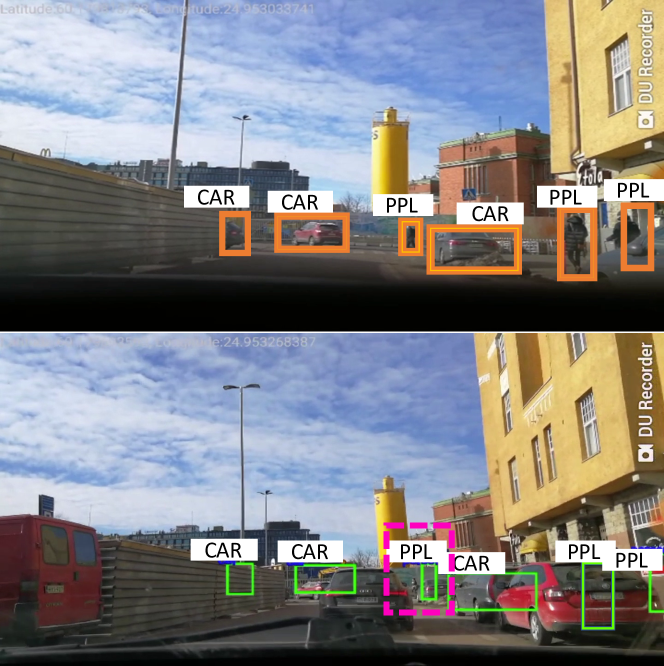
Figure 1: Illustration of a naïve cooperative perception system. A leading vehicle detects objects shown in orange bounding boxes (top figure). These objects are displayed to the driver of the following vehicle in green bounding boxes (bottom figure). AICP filters such objects to only show critical ones (e.g., the pedestrians in the pink bounding box) to reduce on-screen object overload.

The ETSI standards and a few recent works [9, 15] have proposed high-level descriptions of potential filtering rules and mechanisms. However, there are still many topics of dedicated system design that have not been explored. Such is the case of fine-grained protocols that provide efficient data flow with lightweight operations, as well as fast-filtering algorithms that optimize the informativeness of objects in real-time. In this paper, we propose AICP, the first solution that focuses on optimizing informativeness for pervasive cooperative perception systems with efficient filtering at both the network and application layers. AICP identifies, transmits, forwards, and filters objects at scale and displays the most informative ones to the drivers through AR. Such an AR-based system will be useful even for vehicles with level four automation (which experts estimate could be at least ten years from wide scale deployment), since with this automation level drivers may still need to take vehicle control in some complex situations (as compared to fully autonomous level five). Specifically, we make several key contributions as follows.

(1) We propose a system design for AICP. The design includes a dedicated data structure, the vehicular data unit (VDU), designed for informativeness-focused information filtering and transmission. We also describe the full-stack networking protocol, Contextual Multihop Routing (CMR), that the system employs to utilize VDU.

(2) We formulate the informativeness in cooperative perception systems as a multi-level problem, namely the object, message, and vehicle level, and propose a near real-time sorting algorithm based on Mahalanobis distance for fast yet comprehensive filtering. The algorithm provides filtering at the application level to display only the most important information shared by nearby vehicles and thus preventing drivers from information overload.

(3) We implement a proof-of-concept (POC) prototype using a cooperative perception application on an Augmented Reality Head-up Display (ARHUD). We demonstrate the system performance in different contexts via data-driven tests using the data collected with the prototype from road tests. Next, we evaluate the networking performance of AICP at scale. Due to the limit of the testbed, we conducted simulations using a state-of-the-art vehicular network simulator.

We note that AICP is network-agnostic and does not depend on any particular feature of the underlying network. The system can be seamlessly integrated into current and future communication systems such as C-V2X and DSRC.

The rest of the paper is structured as follows. Section II discusses related works and states the key motivations behind AICP. Section III details the system architecture, data structure, and routing protocol. Section IV models the system and formulates the problem. Section V describes the weighted fitness sorting algorithm to calibrate the assessment of informativeness. Section VI shows the POC implementation of AICP and its performance in different contexts. Section VI-C presents the simulation setup and results. Finally, Section VII discusses system limitations and potential solutions, and Section VIII concludes the work.

II Related Work

This work touches on different research areas including cooperative perception, information filtering, and AR in the context of vehicular networks, and so does the related work.

Artificial Intelligence (AI) is at the core of many solutions to increase road safety in modern transportation systems including, for example, autonomous vehicles [16]. Specifically, AI-based perception algorithms help develop an understanding of a vehicle’s surrounding environment through architectures such as convolutional and deep neural networks (CNN and DNN) that perform object detection and recognition. In terms of research in this area, [17] shows that these networks still have significant limitations (that should be considered) and also require optimization of network structure and parameters (e.g., number of layers, filters, and filter sizes) to provide rapid object detection. Similarly, [18] uses deep learning to rapidly segment blind roads and crosswalks to assist visually-impaired people. Furthermore, [18] optimizes existing neural network architectures (e.g., by reducing the number of parameters) to speed up the training and inference, while retaining high model accuracy. However, all these solutions suffer from (inherent) high network complexity, and thus require considerable optimization prior to adoption in real-life, latency-sensitive applications. In comparison, our work does not use a neural network approach but instead relies on basic assumptions about vehicular traffic, and thus does not suffer from this complexity, though as we discuss later neural networks will play a role in our future work.

In terms of general vehicular cooperative perception, Yoon et al. presented a decentralized cooperative perception framework [19]. The work investigates the effects of common inherent limitations of any Vehicle-to-Vehicle (V2V) network, such as the loss of communication and variations in the rate of participating vehicles. The study suggests that the overall perception improves with the vehicle participation rate. However, increasing vehicle participation above a certain optimal rate results in no significant perception improvement, though communication and computation costs in the network increase drastically. Kim et al. proposed a framework addressing several important problems in the field such as map merging, communication uncertainty, and sensor multi-modality [20]. Furthermore, [21] proposed and analyzed different message formats based on ETSI ITS G5 [22] to exchange local sensory data among road participants for collective perception. Thereafter, they proposed a multimodal cooperative perception system with a focus on the engineering feasibility [5], and generalized the work with a mirror neuron-inspired intention awareness algorithm for cooperative autonomous driving [23]. Overall, in contrast, our work focuses on the more pointed problems of information filtering and ranking, which we discuss next, and thus complements these more general works that mainly focus on other problems.

The critical area of filtering mechanisms in vehicular cooperative perception is still very new and has only a few key works. Garlichs et al. [9] in 2019 suggested a set of generation rules to reduce the transmission load while guaranteeing perception capabilities. This proposal was later added to the ETSI standard [7]. Thandavarayan et al. studied the ETSI standards and conducted an in-depth evaluation of the message generation rules [15]. They investigated the trade-off between perception capabilities and communication performance under current standards and concluded that further optimization is needed to reduce information redundancy. To this end, Aoki et al. [24] applied a deep reinforcement learning approach to reduce the information sent between vehicles by only forwarding information about objects that are not likely to have been seen directly by surrounding vehicles themselves. Our work differs in that we focus on only forwarding information about objects that are likely to be important (to receiving vehicles for driver awareness) regardless of whether the object is directly seen by surrounding vehicles. Thus the objective is related but broader and in some sense complementary.

Finally, works in the area of ARHUD, an in-car deployment of AR that visualizes information in the driver’s line-of-sight, are also related. For instance, [25, 8] explore how to share augmented vision between two vehicles. Other studies consider connecting multiple mobile points of view to recompose a scene in 2D or 3D [26]. However, in comparison with our work, these studies mainly focus on image-stitching, and thus overlook aspects that we focus on such as information importance and filtering.

To the best of our knowledge, cooperative augmented vehicular vision at scale still requires additional research on efficient data filtering. Specifically, we believe that AR-powered cooperative perception needs a comprehensive solution to maximize the informativeness of the data shared among vehicles to improve the driving experience while increasing road safety. As such, in this work we propose AICP, a system that lessens the burden on the network through efficient data filtering. As a result, only the most relevant data is broadcast to vehicles, which in turn sort such data to maximize the informativeness that they yield to the driver.

III System Overview

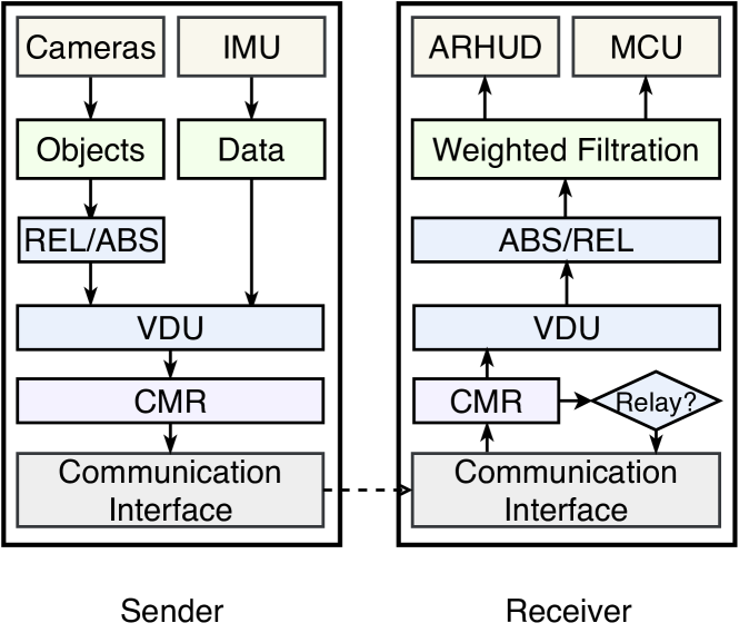
Figure 2: AICP components with information flows. The components include inertial measurement unit (IMU), microprocessor control unit (MCU), relative values (REL), absolute values (ABS), vehicular data unit (VDU), and contextual multihop routing (CMR) protocol.

This section describes the proposed system’s major components, data structures, and routing protocol.

III-A System Architecture

We consider a connected system of vehicles equipped with sensors and wireless communication modules that can collect and share sensory data. We assume the system has capabilities including accurate positioning and localization [27, 28], relative velocity estimation, distance and angle estimation [29], and perspective transformation [8]. In this work, we skip the details of the techniques mentioned above and focus on information filtering. Figure 2 depicts the system architecture including the major data flows between key components. These data flows include:

• IMU sensors in each sender collect sensory data. Each sender detects the objects captured by the onboard cameras and corresponding information such as distance, relative velocity, and moving direction.

• The sender system transforms the object data from relative values to absolute values based on IMU data. For instance, the system transforms the relative velocity of a detected object to absolute velocity by adding its own velocity.

• The data are then encapsulated into VDUs (see Section III-B).

• The sender system encapsulates networking layer information into VDUs according to the CMR (Section III-C).

• The senders and receivers exchange data packets via wireless communication interfaces.

• Each receiver decides whether to forward the received packet based on a network layer filter (see Section III-C).

• Each receiver transforms the absolute values of the objects to relative values based on their IMU data.

• Each receiver performs object resolution to reconcile data (often from multiple senders) that refers to the same object (seen from different sender perspectives).

• Each receiver filters the received VDU based on a filtering algorithm (see Algorithm 2).

• Each receiver ARHUD renders the filtered information through AR to enhance the driver’s situational awareness. The MCU performs maneuvers based on the filtered information.

As such, each vehicle can display the most important situational information in real-time to facilitate safe driving. Next, we describe the VDU and the CMR in detail.

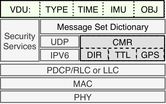
Figure 3: AICP protocol stack including the contextual mutual routing (CMR) and vehicle data unit (VDU) with their specific fields such as location (GPS) and time (TIME). Other generic network layers, such as the link and MAC layers, are shown for reference.

III-B Vehicular Data Unit (VDU)

Figure 3 depicts the overall protocol stack deployed by AICP. AICP is network-agnostic and can be deployed on top of any V2V broadcast-style protocol such as DSRC. CMR is deployed as the routing protocol to provide context-aware routing in a broadcast network environment, in parallel to the traditional UDP/IP stack. Finally, the VDU contains the information required at the application layer. To accelerate data processing during filtering, we propose the vehicular data unit (VDU) for vehicular information encapsulation. A VDU comprises multiple metadata fields, each of which is a key-value pair or key-value map. The metadata fields include:

• TYPE – whether the message is a safety or non-safety application message (pair).

• TIME – the time the information was first created (pair).

• IMU – the information of IMU sensors (map), i.e., {GPS coordinates, velocity, direction, category}.

• OBJ – the information of detected objects (map).

Similar to the SAE J2735 standard [30], the protocol stack defines a message set dictionary to specify the VDU structure and provides sufficient background information to allow vehicle systems to properly interpret the message. Together with the segmented data blocks, the dictionary extends the system compatibility by allowing different VDU structures. The dictionary and VDU also speed up the look-up process of fields such as TIME which can help determine whether the received information is outdated (see Section IV).

III-C Contextual Multihop Routing (CMR)

Vehicle-to-Vehicle (V2V) communication suffers from a short communication range due to signal attenuation caused by obstacles like nearby vehicles and buildings [31]. Therefore, packet forwarding (also known as relaying) is crucial to extend the range over which information can be propagated. As an example, DSRC has a theoretical range of several hundred meters. However, in common non-line-of-sight situations, like intersections, vehicles potentially cannot communicate over distances as short as 60 meters due to obstacle attenuation over the 5.9 GHz band [32].

Additionally, to date, most DSRC and C-V2X standards assume data transmission over a broadcast mechanism. Broadcast transmission allows a vehicle to efficiently forward information to other vehicles in their immediate vicinity. However, broadcast transmission suffers from multiple drawbacks in multihop communication. Unregulated broadcast transmission results in significant data redundancy that affects the system at every level, from increased load and congestion on the transmission medium to large amounts of unnecessary information being forwarded to the drivers. To address these concerns, we introduce CMR as the routing protocol for packet forwarding.

CMR enables the following features.

1. Directional routing in a multihop broadcast transmission. We consider that an object detected by a vehicle is relevant for all immediate neighbor vehicles (accessible within a single hop). In other words, a vehicle that detects an object always forwards the information to neighboring vehicles. However, vehicles that receive such information only process and further forward the information if they are going in the same general direction as the sending vehicle. Specifically, the same general direction is defined as having headings that differ by less than a certain absolute degree threshold (this threshold can vary). This scheme relies on the intuition that vehicles travelling in similar directions will find the same detected objects informative. This represents a trade-off between sending all information and potential congestion (with information loss) or less information (and fewer objects) with less congestion. Though, the scheme can reduce to the former by setting the degree threshold to 180 degrees.

2. Distance and hop limits for geographic relevance After a certain geographic distance, the information also loses relevance (regardless of vehicle direction). Thus vehicles only forward packets if the geographic distance between the vehicle and the sending vehicle is less than a certain threshold. Additionally, as the number of hops acts as a rough proxy for geographic distance (that does not rely on GPS), a hop limit whereby vehicles only forward packets up to a maximum number of hops also helps enforce this geographic distance. The hop limit also helps remove the impact of potential routing loops.

To provide these functions, CMR in this work relies on two different metrics, namely GPS and time-to-live, respectively referring to the coordinates of the detected object and a counter used to enforce the hop limit (see Figure 3). The GPS coordinates of the detected object are encoded over two fields of $32$ bits to achieve the precision of at least a meter.

Note that unlike common routing algorithms such as DV-CAST [33], Greedy Perimeter Stateless Routing (GPSR) [34] and its variants such as [35, 36], CMR focuses on filtering low-informativeness packets instead of improving the communication efficiency. Therefore it is a complementary protocol to the efficiency-focused routing protocols instead of a replacement.

For reference, we detail the basic routing algorithm in Algorithm 1. As mentioned, the parameters of the algorithm include the initial $T$ (time-to-live) value, direction threshold, and distance threshold.

Data: Receiver Direction DIRR, time-to-live T, Receiver Location GPSR, Transmitter Direction DIRT, Transmitter Location GPST, Direction Threshold DT, Distance Threshold D, Packet PKT

1

2T=PKT[T]-1;

3 DIRT=PKT[DIR];

4 GPST=PKT[GPS];

5

6if $\text{T}<0~{}\text{or}~{}|\text{DIRT}-\text{DIRR}|>DT~{}\text{or}~{}\text{Distance}(\text{GPST},\text{GPSR})>D$ then

7       drop(PKT);

8      

9 else

10       forward(PKT);

11       process(PKT);

12      

13 end if

14

Algorithm 1 CMR Directional Routing

IV System Model and Problem Formulation

This section details the system model and the problem of maximizing the informativeness of the displayed objects.

IV-A System Model

The system includes the set $\mathcal{N}=\{1,2,...,N\}$ of $N$ vehicles driving in the considered area, with velocities $\mathcal{V}^{t}=\{v^{t}_{1},v^{t}_{2},...,v^{t}_{N}\}$ at time $t$, respectively. The mobility of the vehicles is exogenous to the system. Each vehicle is equipped with an ADAS or autonomous system consisting of several cameras facing varying directions for comprehensive vision around the vehicle (radar, lidar, and ultrasonic sensors are optional and not a mandatory requirement of AICP), GNSS/IMU for real-time kinematic and positioning, and wireless interfaces (DSRC or C-V2X) for communications with other devices on the road. Messages are sent with a frequency between $1$ and $10$ Hz and the message size is limited to $300$ Bytes, as specified in the C-V2X standard [37, 22]. The encapsulation and decapsulation of the messages follow the protocol standard defined in Figure 3. We model the data propagation from three parallel levels, namely the object level, message level, and vehicle level. AICP decides whether to display an object based on the object level informativeness, to forward a packet based on message level informativeness, and targets optimizing performance based on vehicle level informativeness.

TABLE I: Summary of used notations.

Symbol	Definition
$\mathcal{N}$	Set of all vehicles considered in the system
$\mathcal{V}^{t}$	Set of velocities $\mathcal{V}^{t}=\{v^{t}_{1},\dots,v^{t}_{N}\}$ of $\mathcal{N}$ vehicles
$\textit{T}_{th}$	Initial T (time-to-live) of detected objects in the system
$\vartheta^{O}$	Informativeness of object $O$
$t_{c}$	Time at which a message is created
$\mathcal{I}^{i}(t)$	Informativeness of message $i$ at time $t$
$r$	Decay rate of Informativeness $\mathcal{I}$ over time
$x^{j,i}(t)$	Binary variable indicating if message $i$ is received by vehicle $j$ at time $t$

Object level.  The processing result of each image frame contains a list of detected objects, each of which is defined as $O\triangleq\{D,V,R,C\}$, where $D,V,R,C$ denote the Distance, relative Velocity, diRection and Category of the object, respectively. The rationale of the choice of these parameters is justified by the fact that an object $O$ has a higher chance of causing an accident if (i) it is close to the vehicle, (ii) is getting closer to the vehicle, e.g., catching up with the vehicle from behind or coming right at the vehicle, and (iii) is on the heading direction of the vehicle. Additionally, the rationale for having object categories relies on the fact that certain objects could cause or sustain a greater injury in an accident; e.g., pedestrians and cyclists are more likely to be killed in vehicle accidents compared to vehicle occupants [38].

These parameters are intertwined with each other, and such dynamics are crucial to determine a model upon which we define the informativeness of an object. For instance, the mutual time and space relationship are, in fact, at the basis of modern methodologies to evaluate accidents by analyzing the collision area  [39, 40]. An examination of reported accidents involving autonomous vehicles in California showed that most accidents occur at cross sections in suburban roads, with most accidents reporting rear or front damage [41]. These findings indicate that the direction with which vehicles move greatly affects the probability of an accident, especially if the vehicles are at a short distance from each other. Furthermore, we need to factor in higher informativeness for objects that fall into the people category, for instance.

Upon such considerations, we express the informativeness $\mathcal{I}$ of an object $O$ as:

$${\color[rgb]{0,0,0}{\color[rgb]{0,0,0}\mathcal{I}}^{O}=f(D,V,R,C)}$$ (1)

Since it is not easy to quantify the exact form of function $f$, we instead use a weighted fitness sorting algorithm (Section V-B) to calculate the inter-weight relationships.

More complicated computations such as machine learning along with accident reports of autonomous vehicles[42] can incorporate the understanding of a chain of scenarios; however, they might suffer from additional costs. We leave the investigation of such an approach as possible future work.

Message level.  The messages received by each vehicle may arrive at varying times and with varying delays. In fact, due to the highly time-sensitive nature of the warning messages for assisted driving, vehicles need to establish the timeliness of the message [43]. To this end, the system extracts from the VDU the time at which a given message was created (see TIME in Figure 3), here denoted as $t_{c}$, and uses it to evaluate the timeliness. For a message $i$, its informativeness can be calculated as

$$\mathcal{I}^{i}(t)=\bigg{(}{\color[rgb]{0,0,0}\mathcal{I}}^{i}\Big{(}\dfrac{\textit{T}^{i}(t)}{\textit{T}_{th}}\hskip 2.84526pt(1-r)\Big{)}\bigg{)}^{(t-t_{c}^{i})}$$ (2)

where ${\color[rgb]{0,0,0}\mathcal{I}}^{i}=\max_{o\in O_{i}}{\color[rgb]{0,0,0}\mathcal{I}}^{o}$ denotes the informativeness of message $i$ and $O_{i}$ denotes the detected objects contained in message $i$, $r$ is the rate at which the informativeness of the message decays over time, and $t$ denotes the current time. The decay rate $r$ is strictly connected to the time limit within which such messages are considered up-to-date and relevant. In fact, $r$ is a system parameter that can be tuned for specific conditions.

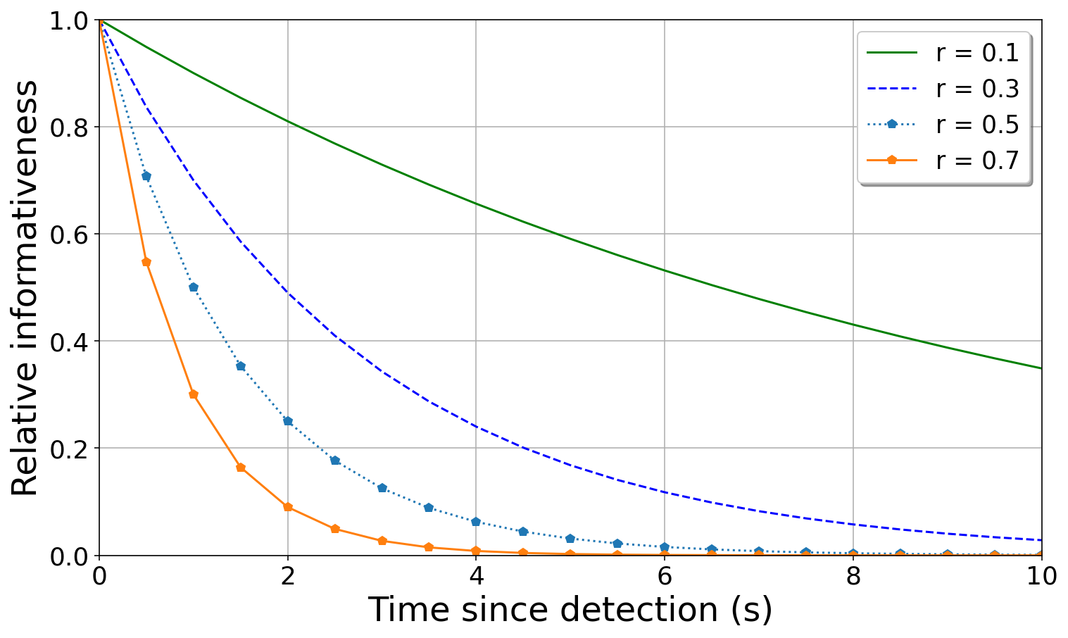
Figure 4: Informativeness of an object relative to its informativeness at detection (t=0) as a function of time elapsed for four different decay rate $r$ parameters.

Figure 4 shows the informativeness of an object as a function of time elapsed since its time of detection (time = $0$) for different decay rates $r$. We call this parameter relative informativeness, and it represents the effect of the decay rate $r$ on the informativeness of an object. This parameter, in fact, dampens an object’s informativeness in addition to that already dictated by the time-to-live $T$ parameter.

A higher decaying rate is required when road conditions change quickly, such as driving at high speeds on the highway. Similarly, we need to relax (i.e., decrease) the decay rate $r$ for conditions with lower speeds such as driving through a city center. For instance, a decay rate of $r=0.3$ halves the informativeness of a message in about $2$ seconds, whereas a decay rate of $0.1$ requires around $6$ seconds to halve the informativeness of an object. Situations such as that of driving in high traffic require low decay rates; for instance, a car driving as slow as $30$ km/h in an urban area would drive a distance of around $50$ m before the informativeness of its generated messages halves, given a decay rate of $0.1$. Keep in mind that $r$ can be further tailored should the sampling frequency of the vehicle’s sensor(s) vary over time. That is, $r$ increases with the sampling frequency due to the fact that a high sampling frequency could lead to detecting the same object(s) during several consecutive times and more frequent message exchanges, and thus a vehicle can afford to discard (the same) old messages faster and avoid network congestion.

According to the proposed ETSI generation rules of CPMs (collective perception messages) [7, 44], objects can be generated and broadcast with a frequency between $100$ and $1000$ ms. As such, object(s) can be re-broadcast already several times before their informativeness halves, ensuring a high degree of diffusion for informative objects and thus messages. Moreover, the decay rate $r$ factors in possible redundancy in the exchange of outdated messages (and thus, objects) among vehicles [45]. That is, it serves as a time delimiter for the broadcast of aged messages, and thus it ensures that only fresh messages are broadcast in the network, similar to [46]. This is especially useful in case there are no or few new detected objects to broadcast, forcing a vehicle to keep broadcasting over time the same outdated messages. As such, the decay rate $r$ serves a dual purpose: first, vehicles transmit and receive only messages (objects) that are fresh and bring a high level of information toward safe driving, and second, it leads to more efficient use of the available channel bandwidth. Relatedly, the use of the max aggregation over object importances when calculating message importance helps ensure that messages with a few important objects but many unimportant objects are not discarded (and thus important objects are not missed). Finally, ${\textit{T}}_{th}$ characterizes the hop limit defined by CMR (see Section III-C). ${\textit{T}}^{i}(t)$ expresses the remaining time-to-live, i.e., the number of hops a message can still be forwarded, of message $i$ at time $t$.

Vehicle level.  At the vehicle level, a vehicle can (i) evaluate a received message as informative and display some objects from that message to the driver and subsequently broadcast the message, (ii) evaluate a received message as irrelevant to themselves but still broadcast the message, or (iii) drop the received message if its information is outdated, and thus not relevant to any vehicle in the network.

Upon receiving a multitude of messages, a vehicle derives the informativeness of the objects within. We assume a vehicle $n\in\mathcal{N}$ receives $\mathsf{M}$ messages at time $t$ from other vehicles in the network and expresses their informativeness as below.

$$\mathcal{I}_{n}(t)=\sum\limits_{\begin{subarray}{c}j=1\\ j\neq n\end{subarray}}^{|\mathcal{N}|}\sum\limits_{\begin{subarray}{c}i=1\end{subarray}}^{\mathsf{{\color[rgb]{0,0,0}M_{j}}}}\bigg{(}{\color[rgb]{0,0,0}\mathcal{I}}^{j,i}s\Big{(}\dfrac{\textit{T}^{i}(t)}{\textit{T}_{th}}\hskip 2.84526pt(1-r)\Big{)}\bigg{)}^{(t-t_{c}^{i,})}x^{j,i}$$ (3)

The binary variable $x^{j,i}$ is $1$ if message $i$ is received by vehicle $j$ ($x^{j,i}=1$), and $0$ otherwise.

The number of received messages (and objects) can increase drastically when a vehicle is in dense traffic, thus displaying all objects would overwhelm the drivers’ field of view and cognitive processing. As such, we next present a mechanism to filter incoming messages by optimizing (i.e., maximizing) their informativeness.

IV-B Problem Formulation

The following formulates an optimization problem for a vehicle to select objects whose informativeness helps to identify imminent risks and thus increase road safety.

Specifically, the problem is defined as below.

$$\max_{j,i}\hskip 5.69046pt\mathcal{I}_{n}(t)$$ (4)

Subject to:

$$\qquad\sum\limits_{\begin{subarray}{c}j=1\\ j\neq n\end{subarray}}^{|\mathcal{N}|}\sum\limits_{\begin{subarray}{c}i=1\end{subarray}}^{\mathsf{{\color[rgb]{0,0,0}M_{j}}}}x^{j,i}\leq L,\hskip 5.69046pt\forall n\in\mathcal{N}$$ (5)

$$\qquad\textit{T}^{i}(t)>0,\hskip 45.52458pt\forall i$$ (6)

$$\qquad x^{i,j}\in\{0,1\},$$ (7)

$$\forall j\in[1,2,...,|\mathcal{N}|],\forall i\in[1,2,...,\mathsf{M}]$$ (8)

The objective function in Eq. (4), defined as the summation of the informativeness of the objects contained in the messages incoming from other vehicles, expresses the collective informativeness that vehicle $n$ conveys at time $t$. Eq. (5) limits the number of selected objects used to convey information to the driver. This allows us to display only clear and limited audio and visual content to a driver [47]. Finally, Eq. (6) specifies that the time-to-live of an object must be, trivially, larger than $0$. Given a suitable value of $L$, AICP selects $L$ objects with the largest informativeness to display to the driver.

We also note that we assume that object resolution (also known as entity resolution) is performed before this informativeness selection step. Object resolution is the process of recognizing that multiple perceived or received objects are actually the same object seen by multiple vehicles at different angles. As this resolution process is a well-known topic in itself, we do not focus further on the process but instead refer to [48], which summarizes different object resolution methods. These methods typically have super-linear but sub-quadratic time complexity with the number of objects and thus should not significantly impact the system performance in practice. We look to study resolution techniques empirically in future work. The following Section V presents the details of the fitness sorting algorithm, which allows such a selection with the time complexity of $\mathcal{O}(\mathsf{M})$.

V Prioritized Sorting Algorithm

In this section, we propose the details of the filtering and prioritized sorting algorithm at the application layer. The algorithm finds the relationships between the attributes that define the informativeness to provide a more comprehensive understanding than the linear weights in Eq. (1).

V-A Warm-up Radix Sorting

We present a warm-up solution that orders the list $\mathbf{O^{v}}$ of objects recently received by a vehicle $v$. The radix sorting algorithm, represented by $Sort()$, arranges the orders of the tuples in $\mathbf{O^{v}}$. Without loss of generality, the algorithm $Sort(a)$ orders the tuples in $\mathbf{O^{v}}$ in ascending order in the attribute $a$. First, we assume the order Distance (D) $\bm{>}_{\text{{I}}}$ relative Velocity (V) $\bm{>}_{\text{{I}}}$ diRection (R) $\bm{>}_{\text{{I}}}$ Category (C) of the four attributes in a tuple. Second, we sort the tuples in $\mathbf{O^{v}}$ by running $Sort(\text{{C}})$, $Sort(\text{{R}})$, $Sort(\text{{V}})$, and $Sort(\text{{D}})$ sequentially. That is, we start sorting from the least significant attribute and move up to the most significant one. We observe that the running time of this solution is about $\mathcal{O}(4n)$ (asymptotic notation) since the running time of the radix sorting algorithm $Sort()$ is $\mathcal{O}(n)$ and we need to process four attributes. However, a drawback to this solution is the assumption of a monotonic relationship between the four attributes, i.e., attribute $a$ is more important than another $b$, regardless of the actual value of $b$.

V-B Weighted Fitness Sorting

To improve the comprehension of the informativeness, we next introduce a more advanced method, which not only considers the impact of the values of the four attributes but also has a faster running time compared to the radix algorithm. To do so, we first must assume that we have a labeled dataset $\mathbb{D}$ in which a large number of tuples $P^{\star}_{i}$, $i=1,2,...,N$ are collected from vehicles and then labeled as either Requires Attention or Does Not Require Attention by human experts on traffic safety analysis. If $L^{\star}_{i}$ denotes the label of tuple $P^{\star}_{i}$, the labeled dataset $\mathbb{D}$ can then be represented as $\mathbb{D}=\{(P^{\star}_{i},L_{i}^{\star}),i=1,2,..,N\}$. For ease of illustration, we assume $L^{\star}_{i}\in\{0,1\}$, where $0$ represents Does Not Require Attention and $1$ represents Requires Attention. We note that the dataset $\mathbb{D}$ could be obtained by using the large volumes of traffic data that connected cars stream back to network centers for data analysis [49, 50]. Furthermore, there are numerous semi-supervised classification algorithms [51, 52] that can be used to build a large dataset $\mathbb{D}$ from a small initial labeled dataset which can be generated manually by traffic experts or even automakers.

Next, we discuss the details of the weighted sorting algorithm. Without loss of generality, we assume that the four attributes D, V, R, and C are represented by the $1$st, $2$nd, $3$rd and $4$th attributes, respectively. Given a tuple $P=(D,V,R,C)$ represented by $P=(x_{1},x_{2},x_{3},x_{4})$, then a labeled tuple in dataset $\mathbb{D}$ is represented by $(x^{\star}_{1},x^{\star}_{2},x^{\star}_{3},x^{\star}_{4},L_{i}^{\star})$. To better define the relationship between the weights in Eq. (1), we define a filter $\mathbb{F}$ which weights the four attributes and their relationship by a $4\times 4$ matrix $M$ shown as follows

$$M=\left[{\begin{array}[]{*{20}{c}}m_{1,1}&{m_{1,2}}&{m_{1,3}}&{m_{1,4}}\\ m_{2,1}&{m_{2,2}}&{m_{2,3}}&{m_{2,4}}\\ m_{3,1}&{m_{3,2}}&{m_{3,3}}&{m_{3,4}}\\ m_{4,1}&{m_{4,2}}&{m_{4,3}}&{m_{4,4}}\end{array}}\right],$$ (9)

where $m_{i,j}>0$ ($i,j\in\{1,2,3,4\}$) is the weight assigned to the relation between the $i$-th and $j$-th attributes. Given a tuple $P=(x_{1},x_{2},x_{3},x_{4})$, filter $\mathbb{F}$ shall compute a fitness $M$ using Mahalanobis distance [53]. The Mahalanobis distance refers to a distance measuring the correlation among the features. It describes the quadratic forms in Gaussian distributions, where the matrix $M$ plays the role of the inverse covariance matrix [54], as follows:

$$\mathbb{F}(P)=P\times M\times P^{\prime}$$ (10)

$$=\left[{x_{1}}\;{x_{2}}\;{x_{3}}\;{x_{4}}\right]\left[{\begin{array}[]{*{5}{c}}m_{1,1}&{m_{1,2}}&{m_{1,3}}&{m_{1,4}}\\ m_{2,1}&{m_{2,2}}&{m_{2,3}}&{m_{2,4}}\\ m_{3,1}&{m_{3,2}}&{m_{3,3}}&{m_{3,4}}\\ m_{4,1}&{m_{4,2}}&{m_{4,3}}&{m_{4,4}}\end{array}}\right]\left[\begin{array}[]{*{5}{c}}x_{1}\\ x_{2}\\ x_{3}\\ x_{4}\end{array}\right]$$ (19)

For ease of illustration, we use $d(P_{i},P_{j})$ to represent the difference of the fitness between two tuples $P_{i}$ and $P_{j}$, i.e.,

$$d(P_{i},P_{j})=(P_{i}-P_{j})\times M\times(P_{i}-P_{j})^{\prime}$$ (20)

Networking layer filtering

1 thread CMR:

2       Determine drop or forward&process PKT according to the CMR protocol (see Section III-C);

3      

Application layer filtering

4 thread Fitness calculation:

5       Update the fitness matrix $M$ (see Eq. (9)) with new datasets according to Eq. (21), offline;

6      

7thread Weighted sorting:

8       Calculate the fitness values of the objects in received messages according to Eq. (10);

9       Sort the fitness values;

10      

11thread Display:

12       Display the first $L$ objects in the sorted queue to achieve Eq. (4) under the constraint of Eq. (5);

13      

Algorithm 2 AICP full-stack filtering algorithm

We find suitable values for the matrix $M$ used by filter $\mathbb{F}$ by leveraging the knowledge from the labeled dataset $\mathbb{D}$. Let $\mathbb{D}_{0}$ represent a subset of $\mathbb{D}$ where each tuple is labeled with $0$, and $\mathbb{D}_{1}=\mathbb{D}\setminus\mathbb{D}_{0}$. The idea is to find a matrix $M^{\star}$ that maximizes the difference of the fitness between the subset $\mathbb{D}_{0}$ and $\mathbb{D}_{1}$, i.e., the fitness of the tuples in $\mathbb{D}_{0}$ shall be as small as possible, while that of the tuples in $\mathbb{D}_{1}$ can be as large as possible, or the vice-versa. More formally, we solve the following optimization problem.

$$\mathop{\arg\max}\limits_{M}\sum\limits_{\begin{subarray}{c}i\neq j,L^{\star}_{i}\neq L^{\star}_{j}\\ {\color[rgb]{0,0,0}i\in\mathbb{D}_{0},j\in\mathbb{D}_{1}}\end{subarray}}d(P^{\star}_{i},P^{\star}_{j})-\sum\limits_{\begin{subarray}{c}i\neq j,L^{\star}_{i}=L^{\star}_{j}\\ {\color[rgb]{0,0,0}i,j\in\mathbb{D}_{0}}\end{subarray}}d(P^{\star}_{i},P^{\star}_{j})$$ (21)

The formula on the left side of the subtraction sign defines the distance between two tuples with different labels (one tuple is labeled $0$ and the other $1$), while the formula on the right side defines the distance between two tuples with the same label (the tuples are labeled either $0$ or $1$). This is a classic metric learning problem for which numerous numerical optimization algorithms are available [55]. This analysis can be carried out offline, and the obtained $M$ matrix can be used to quickly evaluate whether a newly received tuple $P$ needs further processing by calculating its fitness as shown in Eq. (10).

Next, we analyze the time complexity of the weighted sorting solution. As mentioned, obtaining $M$ offline allows us to neglect its computational cost. Upon obtaining $M$, the cost is $\mathcal{O}(1)$ to compute the fitness value of a tuple, and thus $\mathcal{O}(N)$ to calculate the fitness values of the $N$ tuples in the $\mathbf{\mathcal{O}^{v}}$ list. In addition, the cost to sort the fitness values using the radix sorting algorithm is $\mathcal{O}(N)$. Hence, the total computational cost is $\mathcal{O}(2N)$, which is less than that of the warm-up solution (which is $\mathcal{O}(4N)$). Furthermore, the weighted solution is advantageous as it considers the values in each attribute and their relations. As such, we summarize the full-stack filtering algorithm of AICP in Algorithm 2.

VI Evaluation

VI-A Implementation

Following the system design in Section III, we implement a POC prototype of AICP as a sender/receiver system. First, we built a basic prototype that could share vehicular perception in real-time [56]. We deployed the object detector of the sender on a Linux platform with the GPU implementation of Yolo-v5 [29] to conduct object detection in real-time. We used OpenCV for general image processing such as perspective transformation (from one vehicle to another). The detection outputs tuples that consist of the positions and the labels of the objects, as well as confidence scores. The receiver and the other parts of the sender (camera, IMU data collector) were implemented on the Android platform to simulate the hardware and software environment of the vehicular equipment for augmented vision. We used the GPS sensor to report the GPS coordinates of the vehicle, and the monocular camera to capture the front-facing view from the vehicle. We used OpenGL to render the augmented information on top of the camera view. Our implementation operates with a monocular camera (on the Android phone), while vehicles with stereoscopic cameras could make transformations easier. We drove two vehicles equipped with a sender and a receiver respectively across Helsinki city center with one vehicle following the other. The sender detected objects in its line of sight and shared them with the receiver in real-time. We recorded the video including all shared objects without AICP as a benchmark (as shown in the top of Figure 6). Next, we modified the architectures of the sender and receiver to realize the full AICP system as follows.

Sender..  As shown in Figure 5, the sender consists of five components: (i) object detection, (ii) object tracking, (iii) distance estimation, (iv) velocity estimation, and (v) relative/absolute value transform . The system feeds the results to the object tracking component, which maintains a list of the objects tracked in the previous frames. First, such a component calculates the Intersection over Union (IoU), defined as $\frac{\text{area of overlap}}{\text{area of union}}$, between the objects in the previous and the latest frames. Next, it uses a greedy algorithm (quicksort) to sort the similarity according to the IoU scores [57]. The system passes the tracking result to the velocity estimation and distance estimation components simultaneously. The velocity estimation uses the historical positions of an object to estimate the speed and direction of its movement. The distance estimation uses the object’s position and the ratio between the object area and the average size of the object to estimate the distance to the object. As a showcase, we categorize the distance into three classes, namely nearby, middle, and far away. After gathering the objects’ positions, labels, velocities, and distances, the sender broadcasts the messages.

Receiver..  The receiver consists of (i) value transform, (ii) weighted filtration, and (iii) AR display. The receiver applies the weighted fitness sorting algorithm to select the top $L$ informative objects out of the received message and renders them to the driver.

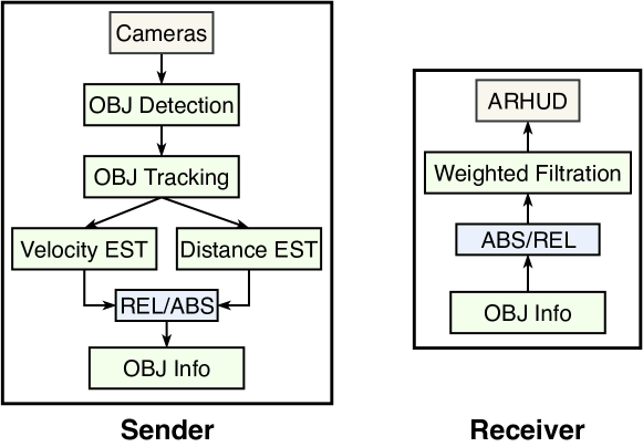
Figure 5: Data flows of the POC prototype system including the practical data processing steps such as object (OBJ) detection, velocity estimation (EST), and relative to absolute value transformation (REL/ABS).

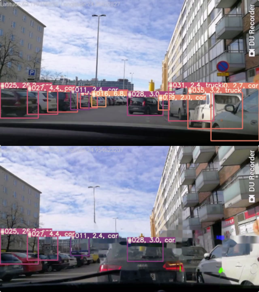
(a) Parking lot.

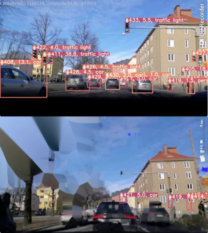
(b) Intersection.

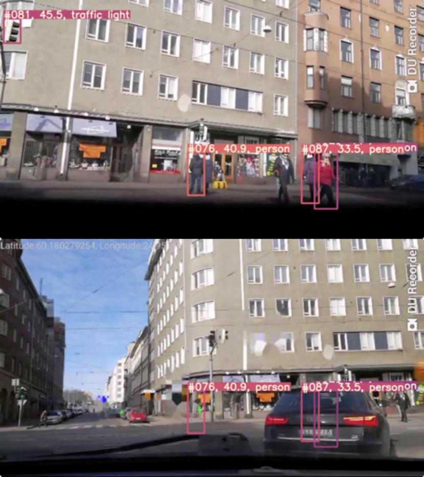
(c) Pedestrians walking across.

Figure 6: POC prototype performance in different contexts. At the top, we see all the objects detected by a sender vehicle, whereas at the bottom, a receiver vehicle sees only the objects that result from our filtering algorithm. For the sake of comprehensibility, we show all the objects that the sender vehicle detects, although a vehicle does not need to render its own objects.

Dataset..  To show the performance of the weighted fitness sorting algorithm (Section V-B), we require that the dataset is labeled. However, due to the difficulty of labeling such data without safety experts, we instead use a heuristic approach just to illustrate the potential performance. Specifically, we label an object as “require attention” when it has a distance of less than 23 meters (safe breaking distance when driving at a safe speed 13 m/s), or velocity larger than 13 m/s, or is a pedestrian and “not require attention” in other cases. As a result, we get 22996 and 52880 objects for the two categories, respectively. We note that the real world distribution might be different but we believe the heuristic provides a reasonable approximation for our purposes.

Algorithm..  We use the metric-learn library contributed by the authors of [58] to implement LMNN for computing the Mahalanobis distance matrix (see Eq. (8) to Eq. (10)). The matrix computation takes 225.79 seconds per 10000 objects. As described in Section V-B, the matrix computation is offline, and thus has no impact on the real-time system performance. Using the learned matrix, each receiver can sort 100 received objects within a millisecond on average. We also open source the code of the weighted fitness sorting algorithm and the 75876-object data extracted from the video.

VI-B Showcase Performance

Table II summarizes the latencies of the processes. As shown, the overall latency in the sender system is only $12.6$ milliseconds and thus has a negligible impact on information dissemination. The additional latency added at the receiver end is mainly the sort latency, which is $\sim 1$ millisecond on average and does not affect the networking performance.

As shown in Figure 6, AICP effectively simplifies and improves the comprehensibility of the cooperative perception system by pruning shared perception information and showing only the most critical objects. In different contexts – e.g., in a parking lot, at an intersection, and with pedestrians crossing the street – the filtered objects that are displayed are much easier to comprehend, and thus facilitate driving. In comparison, cooperative perception systems without AICP would display numerous objects as in Figure 6(a) and Figure 6(b), or uninformative objects such as the traffic lights in Figure 6(c). Note that in different areas the system can improve performance by easily adapting $L$ (the number of selected objects defined in Eq. (5)). For instance, $L$ might be smaller in a parking lot with fewer moving objects in comparison with an intersection that will likely have more moving objects. Cloud services like Google Map can be used for area identification.

TABLE II: Latency breakdown of the POC steps.

	Task	Execution Time (ms)
Sender	Pre-processing	$1.1$
	Object Detection	$6.9$
	Object Tracking	$2.4$
	Velocity & Distance Est.	$1.2$
Receiver	Sorting	$1$
AICP	Overall Latency	$12.6$

Unfortunately, comparing AICP with baselines from literature is difficult because existing works in cooperative perception (see the related works section) typically have related but not matching goals. For example, Aoki et al. [24] aim to reduce V2V network congestion by using deep learning to stop redundant (same object) message transmission. In contrast, we focus on the complementary goal of preventing uninformative message transmission (and therefore, we have different metrics). Additionally, performance comparisons with literature baselines or a purpose-built baseline (such as a deep learning model) would not be overly informative since, as previously mentioned, we do not have a real-world dataset with empirical informativeness labels or rankings. Thus comparisons would not be readily generalizable.

VI-C Simulation

Following the performance of the prototype shown in Section VI-B, we next illustrate the performance of CMR through a larger scale simulation. We open-source the core scripts and datasets of the simulationfn:aicp_code.

Simulation Setup..  As pointed out in Section III-C, CMR focuses on filtering low-informativeness packets rather than improving communication efficiency. To isolate the effect of CMR, we exclude any communication efficiency-focused routing protocols such as GPSR [34] and DV-CAST [33]. Instead, we compare the transmission statistics with and without CMR in city-scale V2V simulations. We select a $4x5$ km rectangular area of London city center and generate traffic utilizing a real-world dataset.

Analogue models.  We simulate the traffic during an off-peak period ($7$ am) and a peak period ($6$ pm) using Veins [59], an open-source framework for running vehicular network simulations. Veins is based on OMNeTpp, an event-based network simulator, and SUMO, a road traffic simulator. We simulate for $60$ seconds. To ensure realism, we employ the two-ray interference model [60] for radio propagation. The model improves over the vanilla two-ray ground model by capturing the ground reflection effects. We also employ the obstacle shadowing model [61] to capture the effects of buildings on signal transmissions. The upper part of Table III details the parameters.

Routing protocol.  We use IEEE 802.11p as the base networking protocol for V2V communications. Following the design of CMR, we set the hop limit of each message to $2$, the maximum concerned source distance to $100$ meters, and the maximum heading direction difference between the source vehicle and the receiver to $30$ degrees. The C-V2X standard [37, 22] recommends a message frequency between 1 and 10 Hz. To test the baseline performance, we let each vehicle broadcast VDUs at 10 Hz. From the POC test, we observe 10 objects per image on average. Thus, the average VDU packet size is set to 102 bytes. Table III and Table IV detail the CMR parameters and packet format.

TABLE III: Simulation parameters

Simulation Parameter	Value
Radio Propagation Model	Two-Ray Interference Model [60]
Shadowing Model	Obstacle Shadowing Model [61]
IEEE 802.11p Bit Rate	$6$ Mbps
Transmission Power	$20$ mW
Noise Floor	$-98$ dBm
Antenna Height	$1.5$ m
Antenna Type	Front-Rearfn:aicp_code
Number of Vehicles	61 (7am), 212 (6pm)fn:aicp_code
[62]
Simulation Area	$4000$x$5000$ m
Simulation Time	$60$ s

CMR Parameter	Value
Beacon Generation Rate	$10$ Hz
Hop Limit	$2$
Max Source Heading Direction Deviation	$30$°
Max Source Distance	$100$ m
Packet Size	$102$ Bytes

TABLE IV: Packet format ($102$ B)

Field	Metadata	Size (Byte)
Object	ID	$2$
	position_x	$1$
	position_y	$1$
	velocity	$1$
	distance	$1$
	label	$1$
	confidence	$1$
Vehicle	IMUs	$12$
	Timestamp	$2$
	GPS	$8$

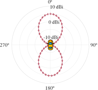
Figure 7: Front-Rear antennae radiation pattern (view from above with vehicle facing north) in dBi.

Results. Due to the dense traffic in the selected area, the average vehicle speed in the simulation period is about $6$ km/h, thus reflecting the lower bound of system performance under extremely congested scenarios.

Antenna type.  As demonstrated by [63, 64], angled antennae, compared to idealistic isotropic antennas, can significantly change the vehicular network dynamics. Therefore, we propose to use a Front-Rearfn:aicp_code antenna to complement the CMR protocol. Recall that CMR prioritizes data sent by source vehicles traveling in a similar direction as the receiver. As shown in Figure 7, Front-Rear amplifies the signal in the forward and rear directions while reducing the transmission range on the sides. Hence, Front-Rear reduces the packets sent from vehicles driving on the sides and reduces the burden of the filters. Front-Rear can be deployed similarly as Patch [63], i.e., mounted to the front of the right and left side mirrors and the right and left side of the rear windshield.

(a)

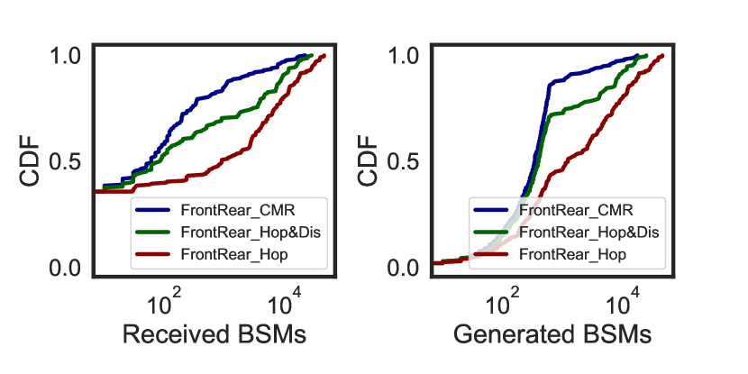
(b)

Figure 8: CDF of received and generated basic safety messages using a Front-Rear antenna and different filter mechanisms: the proposed CMR, Hop&Dis filter with 2 hops and 100 m distance, and Hop filter with 2 hops at 8(a) 7 am and 8(b) 6 pm.

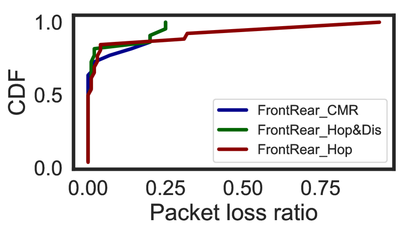
(a)

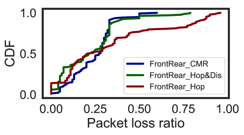
(b)

Figure 9: CDF of packet loss ratio with different filters: the proposed CMR, Hop&Dis filter with 2 hops and 100 m distance, and Hop filter with 2 hops at 9(a) 7 am and 9(b) 6 pm.

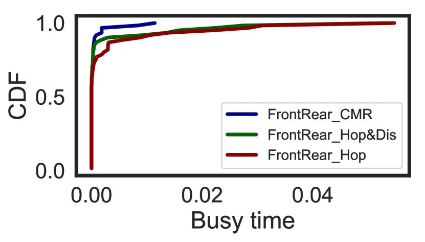
(a)

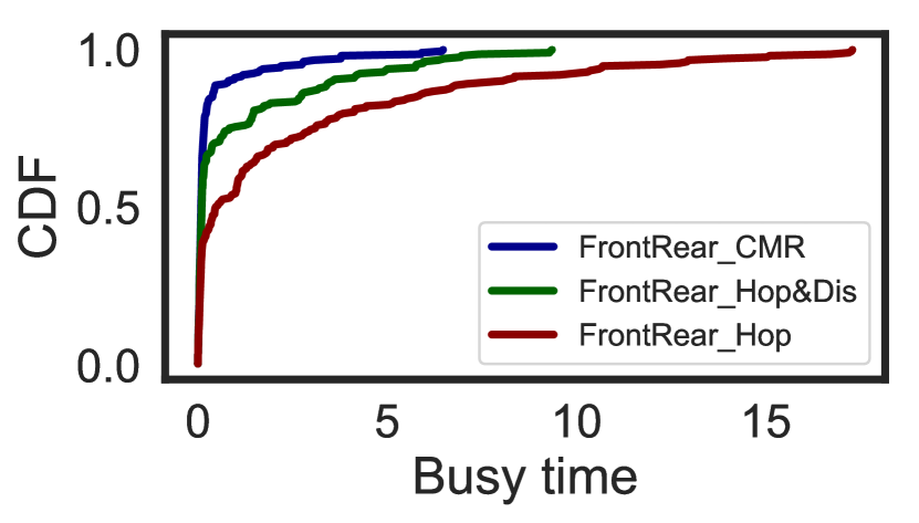
(b)

Figure 10: CDF of channel busy time with different filters: the proposed CMR, Hop&Dis filter with 2 hops and 100 m distance, and Hop filter with 2 hops at 10(a) 7 am and 10(b) 6 pm.

Filters.  We compare CMR with two other classic filters: hop and distance limit (Hop&Dis), and hop limit only (Hop). Figure 8 shows the empirical cumulative distributions of the number of generated and received basic safety messages (BSMs) by vehicles when using different filters. Figure 9 and Figure 10 show the empirical cumulative distributions of the packet loss ratio and channel busy time experienced by the vehicles. As summarized in Table V, CMR effectively filters considerably more packets in both off-peak and peak periods compared to Hop&Dis (-72% / -61%) or only Hop (-80% / -81%). Furthermore, CMR has a slightly higher packet loss ratio than Hop&Dis but shows considerably less channel busy time than the other two filters in the peak period (-61% and -83%, respectively).

TABLE V: Simulation results (7 am / 6 pm).

Filter	Received BSMs	Busy time (s)	Packet loss
CMR	83 / 1024	0 / 0.39	0.31 / 0.63
Hop&Dis	303 / 2630	0 / 1.01	0.30 / 0.54
Hop	416 / 5652	0 / 2.41	0.09 / 0.71

As mentioned in Section III, AICP focuses on informativeness and thus employs CMR to filter low-informativeness packets. We implement CMR in Veins with only five lines of code and argue the CMR would also be lightweight in reality. Hence, CMR could be easily integrated into routing protocols focusing on communication efficiency improvements.

VII Discussion

Due to the stochastic nature of human driving and the driving environment, packets containing information about a certain object may not reach their destination consistently. For instance, vehicles may move in and out of the transmission region (hop limit), and thus only receive a fraction of the packets concerning a given object. Similarly, the filtering algorithm may select different objects to display on each round. As such, the objects displayed on-screen may flicker and thus significantly degrade the driving experience by distracting the driver and deteriorating the received information quality [65].

As this contradicts the goals of our proposed AICP, in future work we look to explore potential solutions such as an object persistence delay. In other words, once an object is displayed on-screen, the object remains displayed for a fixed amount of time, regardless of updates and potential filtering. This delay should be set to a value high enough in order not to distract the driver with high frequency flickering. However, longer delays may lead to a cluttering of the display with objects of low informativeness. A delay between 500 ms to 2 s could represent an acceptable trade-off to preserve high informativeness while avoiding flickering.

Beyond the object flickering, other user-centric and human-computer interaction (HCI) aspects of the AICP system or potential system extensions could also be a target of future work. In particular, we could consider two different aspects. First, multi-modal cues (visual, audio, and tactile [47, 66]) could ease the driver’s cognitive load and improve driving performance when the driver’s attention primarily focuses on the road [67]. Second, we could evaluate the placement of certain visual contents (e.g., focal vs. peripheral placement [68, 69]) to determine the optimal positioning for driving performance.

Finally, our system focuses on fast information filtering and it relies on reasonable heuristics (e.g., objects physically closer to the vehicle are more informative) to determine the informativeness of any specific object near the vehicle in near real-time. However, given that a group of vehicles is an interacting set of agents, other methods might help predict object informativeness in more complex scenarios such as, for instance, an accident caused by a time series of events. Therefore, in future work, we will examine a data-based deep learning approach that accounts for such complex scenarios. Though importantly, compared to such an approach, AIPC will still likely have some practical advantages such as simplicity, explainability, and lower latency.

VIII Conclusion

In this work, we propose AICP, the first solution that focuses on optimizing informativeness for pervasive cooperative perception systems with efficient filtering at both the network and application layers. To facilitate system networking, we also propose a networking protocol stack that includes VDU and CMR, a dedicated data structure and a lightweight routing protocol, respectively, both designed specifically for informativeness-focused applications. We also formulate the informativeness problem in cooperative perception systems from several different levels and propose a prioritized sorting algorithm for fast information-based filtering. Overall, AICP displays only the most important information shared by nearby vehicles, and thus eases the understanding of the surrounding for the drivers. We implement a POC of our proposal with ARHUD and show that the system has negligible additional processing latency ($12.6$ ms). Additionally, simulation results show that CMR effectively filters less relevant packets, and thus considerably improves the channel availability of the vehicles.

References

- [1] M. P. Muresan and S. Nedevschi, “Multi-object tracking of 3d cuboids using aggregated features,” in 2019 IEEE 15th International Conference on Intelligent Computer Communication and Processing (ICCP), 2019.
- [2] H. Kim, J. Cho, D. Kim, and K. Huh, “Intervention minimized semi-autonomous control using decoupled model predictive control,” in 2017 IEEE Intelligent Vehicles Symposium (IV), 2017, pp. 618–623.
- [3] A. Arıkan, A. Kayaduman, S. Polat, Y. Şimşek, I. C. Dikmen, H. G. Bakır, T. Karadağ, and T. Abbasov, “Control method simulation and application for autonomous vehicles,” in 2018 International Conference on Artificial Intelligence and Data Processing (IDAP), 2018, pp. 1–4.
- [4] A. Rauch, F. Klanner, R. Rasshofer, and K. Dietmayer, “Car2x-based perception in a high-level fusion architecture for cooperative perception systems,” in 2012 IEEE Intelligent Vehicles Symposium, 2012.
- [5] S.-W. Kim, B. Qin, Z. J. Chong, X. Shen, W. Liu, M. H. Ang, E. Frazzoli, and D. Rus, “Multivehicle cooperative driving using cooperative perception: Design and experimental validation,” IEEE Transactions on Intelligent Transportation Systems, vol. 16, no. 2, pp. 663–680, 2015.
- [6] ETSI, “Intelligent Transport Systems (ITS); Cooperative Perception Services (CPS),” ETSI TS. 103 324, Early draft, 2020.
- [7] ETSI, “ETSI TR 103 562 - Intelligent Transport Systems (ITS); Vehicular Communications; Basic Set of Applications; Analysis of the Collective Perception Service (CPS),” Tech. Rep. V2.1.1, 2019.
- [8] H. Qiu, F. Ahmad, F. Bai, M. Gruteser, and R. Govindan, “Avr: Augmented vehicular reality,” in Proceedings of the 16th Annual International Conference on Mobile Systems, Applications, and Services, 2018, pp. 81–95.
- [9] K. Garlichs, H.-J. Günther, and L. C. Wolf, “Generation rules for the collective perception service,” in 2019 IEEE Vehicular Networking Conference (VNC), 2019, pp. 1–8.
- [10] P. Zhou, W. Zhang, T. Braud, P. Hui, and J. Kangasharju, “Arve: Augmented reality applications in vehicle to edge networks,” in Proceedings of the 2018 Workshop on Mobile Edge Communications, 2018.
- [11] ——, “Enhanced augmented reality applications in vehicle-to-edge networks,” in 22nd Conference on Innovation in Clouds, Internet and Networks and Workshops (ICIN). IEEE, 2019.
- [12] K.-Y. Lam, L.-H. Lee, and P. Hui, “A2w: Context-aware recommendation system for mobile augmented reality web browse,” in The 29th ACM International Conference on Multimedia (ACM MM’21), 2021.
- [13] W. Liu, J. Gori, O. Rioul, M. Beaudouin-Lafon, and Y. Guiard, “How relevant is hick’s law for hci?” in CHI, 2020.
- [14] R. Schweickert and B. Boruff, “Short-term memory capacity: magic number or magic spell?” Journal of experimental psychology. Learning, memory, and cognition, 1986.
- [15] G. Thandavarayan, M. Sepulcre, and J. Gozalvez, “Analysis of message generation rules for collective perception in connected and automated driving,” in 2019 IEEE Intelligent Vehicles Symposium (IV), 2019.
- [16] Y. Ma, Z. Wang, H. Yang, and L. Yang, “Artificial intelligence applications in the development of autonomous vehicles: a survey,” IEEE/CAA Journal of Automatica Sinica, vol. 7, no. 2, pp. 315–329, 2020.
- [17] P. M. Kebria, A. Khosravi, S. M. Salaken, and S. Nahavandi, “Deep imitation learning for autonomous vehicles based on convolutional neural networks,” IEEE/CAA Journal of Automatica Sinica, vol. 7, no. 1, pp. 82–95, 2019.
- [18] Z. Cao, X. Xu, B. Hu, and M. Zhou, “Rapid detection of blind roads and crosswalks by using a lightweight semantic segmentation network,” IEEE Transactions on Intelligent Transportation Systems, 2020.
- [19] D. D. Yoon, B. Ayalew, and G. M. N. Ali, “Performance of decentralized cooperative perception in v2v connected traffic,” IEEE Transactions on Intelligent Transportation Systems, 2021.
- [20] S.-W. Kim, Z. J. Chong, B. Qin, X. Shen, Z. Cheng, W. Liu, and M. H. Ang, “Cooperative perception for autonomous vehicle control on the road: Motivation and experimental results,” in 2013 IEEE/RSJ International Conference on Intelligent Robots and Systems, 2013.
- [21] H.-J. Günther, R. Riebl, L. Wolf, and C. Facchi, “Collective perception and decentralized congestion control in vehicular ad-hoc networks,” in 2016 IEEE Vehicular Networking Conference (VNC), 2016, pp. 1–8.
- [22] ETSI, “Intelligent Transport Systems (ITS); ITS-G5 Access Layer Specification for Intelligent Transport Systems Operating in the 5 GHz Frequency Band,” ETSI TR. 302 663 V1.3.0, 2019.
- [23] S.-W. Kim and W. Liu, “Cooperative autonomous driving: A mirror neuron inspired intention awareness and cooperative perception approach,” IEEE Intelligent Transportation Systems Magazine, vol. 8, no. 3, pp. 23–32, 2016.
- [24] S. Aoki, T. Higuchi, and O. Altintas, “Cooperative perception with deep reinforcement learning for connected vehicles,” in 2020 IEEE Intelligent Vehicles Symposium (IV). IEEE, pp. 328–334.
- [25] H. Qiu, F. Ahmad, R. Govindan, M. Gruteser, F. Bai, and G. Kar, “Augmented vehicular reality: Enabling extended vision for future vehicles,” in Proceedings of the 18th International Workshop on Mobile Computing Systems and Applications, 2017, pp. 67–72.
- [26] Q. Chen, S. Tang, Q. Yang, and S. Fu, “Cooper: Cooperative perception for connected autonomous vehicles based on 3d point clouds,” in 2019 IEEE 39th International Conference on Distributed Computing Systems (ICDCS), 2019, pp. 514–524.
- [27] R. W. Wolcott and R. M. Eustice, “Fast lidar localization using multiresolution gaussian mixture maps,” in 2015 IEEE International Conference on Robotics and Automation (ICRA), 2015, pp. 2814–2821.
- [28] A. Y. Hata and D. F. Wolf, “Feature detection for vehicle localization in urban environments using a multilayer lidar,” IEEE Transactions on Intelligent Transportation Systems, vol. 17, no. 2, pp. 420–429, 2016.
- [29] G. J. et al., “ultralytics/yolov5: v3.0,” 2020. [Online]. Available: https://doi.org/10.5281/zenodo.3983579
- [30] SAE International, “V2x communications message set dictionary,” 2020.
- [31] L. telcom, “In-car mobile signal attenuation measurements,” LS telcom UK, Tech. Rep, 2017.
- [32] M. Noor-A-Rahim, G. M. N. Ali, H. Nguyen, and Y. L. Guan, “Performance analysis of ieee 802.11 p safety message broadcast with and without relaying at road intersection,” IEEE Access, vol. 6, pp. 23 786–23 799, 2018.
- [33] O. K. Tonguz, N. Wisitpongphan, and F. Bai, “Dv-cast: A distributed vehicular broadcast protocol for vehicular ad hoc networks,” IEEE Wireless Communications, vol. 17, no. 2, pp. 47–57, 2010.
- [34] B. Karp and H.-T. Kung, “Gpsr: Greedy perimeter stateless routing for wireless networks,” in Proceedings of the 6th annual international conference on Mobile computing and networking, 2000, pp. 243–254.
- [35] C. Lochert, M. Mauve, H. Füßler, and H. Hartenstein, “Geographic routing in city scenarios,” ACM SIGMOBILE mobile computing and communications review, vol. 9, no. 1, pp. 69–72, 2005.
- [36] F. Granelli, G. Boato, D. Kliazovich, and G. Vernazza, “Enhanced gpsr routing in multi-hop vehicular communications through movement awareness,” IEEE Communications Letters, vol. 11, no. 10, pp. 781–783, 2007.
- [37] GSMA, “Cellular Vehicle-to-everything; Enabling intelligent transport.”
- [38] M. Peden, R. Scurfield, D. Sleet, A. A. Hyder, C. Mathers, E. Jarawan, A. Hyder, D. Mohan, and E. Jarawan, World report on road traffic injury prevention. World Health Organization, 2004.
- [39] I. Dirnbach, T. Kubjatko, E. Kolla, J. Ondruš, and Ž. Šarić, “Methodology designed to evaluate accidents at intersection crossings with respect to forensic purposes and transport sustainability,” Sustainability, 2020.
- [40] T. Higuchi, M. Giordani, A. Zanella, M. Zorzi, and O. Altintas, “Value-anticipating v2v communications for cooperative perception,” in 2019 IEEE Intelligent Vehicles Symposium (IV). IEEE, 2019.
- [41] F. M. Favarò, N. Nader, S. O. Eurich, M. Tripp, and N. Varadaraju, “Examining accident reports involving autonomous vehicles in california,” PLoS one, 2017.
- [42] H. Caesar, V. Bankiti, A. H. Lang, S. Vora, V. E. Liong, Q. Xu, A. Krishnan, Y. Pan, G. Baldan, and O. Beijbom, “nuscenes: A multimodal dataset for autonomous driving,” in CVPR, 2020.
- [43] B. Hannah Topliss, C. Harvey, and G. Burnett, “How long can a driver look? exploring time thresholds to evaluate head-up display imagery,” in AutomotiveUI, 2020.
- [44] G. Thandavarayan, M. Sepulcre, and J. Gozalvez, “Generation of cooperative perception messages for connected and automated vehicles,” IEEE Transactions on Vehicular Technology, vol. 69, no. 12, pp. 16 336–16 341, 2020.
- [45] G. Thandavarayan, M. Sepulcre, and J. Gozalvez, “Redundancy mitigation in cooperative perception for connected and automated vehicles,” in 2020 IEEE 91st Vehicular Technology Conference, 2020.
- [46] L. Corneo, C. Rohner, and P. Gunningberg, “Age of information-aware scheduling for timely and scalable internet of things applications,” in IEEE Conference on Computer Communications, 2019, pp. 2476–2484.
- [47] N. N. Correia and A. Tanaka, “Avui: Designing a toolkit for audiovisual interfaces,” in CHI, 2017.
- [48] G. Papadakis, D. Skoutas, E. Thanos, and T. Palpanas, “Blocking and filtering techniques for entity resolution: A survey,” ACM Computing Surveys (CSUR), 2020.
- [49] N. Cheng, F. Lyu, J. Chen, W. Xu, H. Zhou, S. Zhang, and X. Shen, “Big data driven vehicular networks,” IEEE Network, vol. 32, no. 6, pp. 160–167, 2018.
- [50] D. Sun, K. Zhang, and S. Shen, “Analyzing spatiotemporal traffic line source emissions based on massive didi online car-hailing service data,” Transportation Research Part D: Transport and Environment, vol. 62, pp. 699–714, 2018.
- [51] N. F. F. D. Silva, L. F. Coletta, and E. R. Hruschka, “A survey and comparative study of tweet sentiment analysis via semi-supervised learning,” ACM Computing Surveys (CSUR), vol. 49, no. 1, pp. 1–26, 2016.
- [52] I. Triguero, S. García, and F. Herrera, “Self-labeled techniques for semi-supervised learning: taxonomy, software and empirical study,” Knowledge and Information systems, vol. 42, no. 2, pp. 245–284, 2015.
- [53] R. Maesschalck, D. Jouan-Rimbaud, and D. Massart, “The mahalanobis distance,” Chemometrics and Intelligent Laboratory Systems, vol. 50, pp. 1–18, 2000.
- [54] K. Q. Weinberger and L. K. Saul, “Distance metric learning for large margin nearest neighbor classification,” J. Mach. Learn. Res., vol. 10, p. 207–244, Jun. 2009.
- [55] B. Kulis et al., “Metric learning: A survey,” Foundations and Trends in Machine Learning, 2013.
- [56] P. Zhou, T. Braud, A. Zavodovski, Z. Liu, X. Chen, P. Hui, and J. Kangasharju, “Edge-facilitated augmented vision in vehicle-to-everything networks,” IEEE Transactions on Vehicular Technology, vol. 69, no. 10, pp. 12 187–12 201, 2020.
- [57] E. Bochinski, V. Eiselein, and T. Sikora, “High-speed tracking-by-detection without using image information,” in AVSS, 2017.
- [58] W. De Vazelhes, C. Carey, Y. Tang, N. Vauquier, and A. Bellet, “metric-learn: Metric learning algorithms in python,” Journal of Machine Learning Research, 2020.
- [59] C. Sommer, R. German, and F. Dressler, “Bidirectionally Coupled Network and Road Traffic Simulation for Improved IVC Analysis,” TMC, 2011.
- [60] C. Sommer and F. Dressler, “Using the right two-ray model ? a measurement-based evaluation of phy models in vanets,” 2011.
- [61] C. Sommer, D. Eckhoff, and F. Dressler, “Ivc in cities: Signal attenuation by buildings and how parked cars can improve the situation,” IEEE Transactions on Mobile Computing, vol. 13, no. 8, pp. 1733–1745, 2014.
- [62] P. Zhou, “AICP simulation code and datasets,” 2021. [Online]. Available: https://github.com/pengyuan-zhou/AICP
- [63] D. Kornek, M. Schack, E. Slottke, O. Klemp, I. Rolfes, and T. Kürner, “Effects of antenna characteristics and placements on a vehicle-to-vehicle channel scenario,” in 2010 IEEE International Conference on Communications Workshops, 2010, pp. 1–5.
- [64] D. Eckhoff, A. Brummer, and C. Sommer, “On the impact of antenna patterns on vanet simulation,” in 2016 IEEE Vehicular Networking Conference (VNC), 2016, pp. 1–4.
- [65] A. Colley, J. Häkkilä, B. Pfleging, and F. Alt, “A design space for external displays on cars,” in AutomotiveUI, 2017.
- [66] S. Onimaru and M. Kitazaki, “Visual and tactile information to improve drivers’ performance,” in IEEE Virtual Reality Conference, 2010.
- [67] S. Onimaru, T. Uraoka, N. Matsuzaki, and M. Kitazaki, “Cross-modal information display to improve driving performance,” in VRST, 2008.
- [68] R. Häuslschmid, S. Osterwald, M. Lang, and A. Butz, “Augmenting the driver’s view with peripheral information on a windshield display,” in IUI, 2015.
- [69] I. Chaturvedi, F. H. Bijarbooneh, T. Braud, and P. Hui, “Peripheral vision: a new killer app for smart glasses,” in IUI, 2019.