Pore-scale Mixing and the Evolution of Hydrodynamic Dispersion in Porous Media

Abstract

We study the interplay of pore-scale mixing and network-scale advection through heterogeneous porous media, and its role for the evolution and asymptotic behavior of hydrodynamic dispersion. In a Lagrangian framework, we identify three fundamental mechanisms of pore-scale mixing that determine large scale particle motion, namely, the smoothing of intra-pore velocity contrasts, the increase of the tortuosity of particle paths, and the setting of a maximum time for particle transitions. Based on these mechanisms, we derive a theory that predicts anomalous and normal hydrodynamic dispersion based on the characteristic pore length, Eulerian velocity distribution and Péclet number.

Transport of dissolved substances through porous media is determined by the complexity of the velocity field in the pore space and diffusive mass transfer within and between pores. The interplay of diffusive pore-scale mixing and spatial flow variability are key for the understanding of transport and reaction phenomena in natural and engineered porous media Brenner and Edwards (1993); Sahimi (2011); Valocchi et al. (2018) with diverse applications ranging from groundwater contamination and geological carbon dioxide storage Niemi et al. (2017), to the design of batteries Maggiolo et al. (2020) and transport in brain microcirculation Berg et al. (2019).

Therefore, hydrodynamic transport has been the focus of research over decades in different disciplines de Josselin de Jong (1958); Saffman (1959); Bear (1972); Brenner and Edwards (1993); Isichenko (1992); Sahimi (2011). Still, as outlined in the following, questions of fundamental nature remain concerning both the evolution of hydrodynamic dispersion, and the dependence of asymptotic hydrodynamic dispersion coefficients on the Péclet number, which compares the diffusion and advection times over a typical pore length. Anomalous dispersion phenomena Bouchaud and Georges (1990) have been observed in laboratory experiments Moroni and Cushman (2001); Levy and Berkowitz (2003); Seymour et al. (2004); Morales et al. (2017); Carrel et al. (2018); Souzy et al. (2020), field scale tracer tests  Gouze et al. (2008); Haggerty and Gorelick (1995), and numerical simulations in different types of porous medium and rock structures Bijeljic et al. (2011, 2013); De Anna et al. (2013); Icardi et al. (2014); Kang et al. (2014); Meyer and Bijeljic (2016); Li et al. (2018). They cannot be described by a single constant hydrodynamic dispersion coefficient. The asymptotic concept of hydrodynamic dispersion models particle displacements due to velocity fluctuations as Brownian motion and thus implicitly assumes that all particles have access to the full fluctuation spectrum at each moment, that is, they can be considered as statistically equal. In a porous medium, however, velocities vary on length scales engraved in the pore structure, and thus, particle transitions over regions of low velocity can be much longer than over regions of high velocity. Statistical equivalence can only be achieved at times larger than the largest transition time scale. Thus, anomalous behaviors can be traced back to broad distributions of mass transfer time scales related to wide spectra of pore-scale flow velocities.

This phenomenology lies at the heart of non-local transport theories such as multi-trapping and continuous time random walk (CTRW), which have been used to model anomalous and intermittent pore-scale transport behaviors Bijeljic et al. (2011); Liu and Kitanidis (2012); De Anna et al. (2013); Kang et al. (2014); Dentz et al. (2018); Puyguiraud et al. (2019a); Nissan and Berkowitz (2019); Souzy et al. (2020). However, current approaches are limited to purely advective transport, or need to be constrained by the measurement of particle transition times. The quantitative relation between pore-scale mixing, network scale flow and the evolution of hydrodynamic dispersion remains elusive. The pioneering works of de Josselin de Jong (1958) and Saffman (1959) use the concept of particle transition times to derive expressions for the asymptotic hydrodynamic dispersion coefficients. Still, and in spite of numerous theoretical and numerical studies Koch and Brady (1985); Scheven (2013); Bijeljic and Blunt (2006), the dependence of hydrodynamic dispersion on the Péclet number remains an open issue.

We address these fundamental questions by identifying and quantifying the key mechanisms of pore-scale mixing and network-scale flow variability in a stochastic model for the prediction of hydrodynamic dispersion. We derive a theory that explains the temporal evolution of dispersion and the dependence of its asymptotic behavior on the Péclet number based on the Eulerian flow statistics, diffusion and the characteristic velocity length scale. The theoretical developments are supported and validated by direct numerical simulations (DNS) of flow and transport in a $3$-dimensional digitized Berea sandstone sample (Fig. 1) obtained using X-Ray microtomography si . The medium displays strong pore-scale heterogeneity that gives rise to a broad distribution of flow speeds illustrated in Figure 2a. We consider transport at different Péclet numbers, which are varied by changing the average flow rate. The molecular diffusion coefficient is set equal to $D_{m}=10^{-9}$ m²/s. The Péclet number is here defined by $Pe=\langle v_{e}\rangle\ell_{0}/D_{m}$, where $\ell_{0}$ is the average pore length and $\langle v_{e}\rangle$ the average Eulerian flow speed.

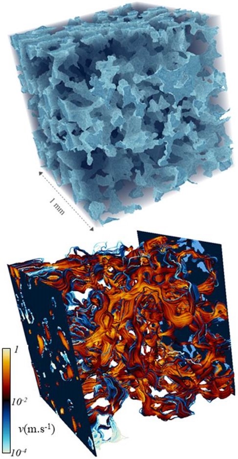
Figure 1: Three-dimensional structure of a Berea sandstone sample. The top panel highlights the void space in shades of blue. The lines in the bottom panel show particle paths. The color scheme indicates particle speeds from (white-blue-black-orange) low to high.

Figure 3 illustrates the impact of flow heterogeneity and diffusion at different $Pe$. It shows on the one hand anomalous hydrodynamic dispersion manifest in heavy-tailed arrival time distributions $f(t)$ and super-diffusive growth of the longitudinal displacement variance $\sigma^{2}(t)$, and on the other hand cross-overs to asymptotically Fickian behaviors (Figs. 3a and b). Streamwise dispersion in the asymptotic regime is characterized by the constant hydrodynamic dispersion coefficient $D^{\ast}$, whose non-linear dependence on the Péclet number is shown in Figure 3c. These features, which result from the complex interplay of flow heterogeneity, diffusion, and geometry are generally observed in laminar flows through porous media and networks Bijeljic et al. (2011).

In order to understand the mechanisms that cause these behaviors, we consider particle motion along the tortuous paths in the void space of a porous medium as illustrated in Figure 1. The flow speed along streamlines varies over the correlation scale $\ell_{v}$ imprinted in the medium geometry and flow structure Morales et al. (2017); Puyguiraud et al. (2019b); $\ell_{v}$ is typically larger than the geometric pore length $\ell_{0}$ due to the tortuosity of the streamlines. We model motion along particle pathways through discrete spatial steps along conducts of length $\ell_{v}$ such that subsequent particle speeds $\{v_{n}\}$ and therefore transition times $\{\tau_{n}\}$ along a path can be considered as independent random variables. The distance $s_{n}$ and transport time $t_{n}$ of a particle along a tortuous pathway are described by the stochastic process

$$s_{n+1}=s_{n}+\ell_{v}, t_{n+1}=t_{n}+\tau_{n}.$$ (1)

The travel distance $s(t)$ along a particle path in this coarse-grained picture is given by $s(t)=s_{n_{t}}$, where $n_{t}=\max(n|t_{n}\leq t)$. This picture is equivalent to representing the pore space as a network of connected conducts of length $\ell_{v}$ and average flow speeds $v_{m}$ Saffman (1959), whose intersections correspond to the turning points of the process (1).

For purely advective transport, particles move along streamlines by the local Eulerian flow speed. Motion along streamlines is projected onto streamwise motion by advective tortuosity $\chi_{a}=\langle v_{e}\rangle/\overline{u}$, which is equal to the ratio between the average Eulerian flow speed $\langle v_{e}\rangle$ and average streamwise flow velocity $\overline{u}$ Koponen et al. (1996); Ghanbarian et al. (2013); Puyguiraud et al. (2019a). In the presence of pore-scale diffusion this is different. First, during a transition over a conduct, particles sample the flow speeds across streamlines. Thus, the actual particle speed is different from the local flow speed along a streamline. Second, diffusion sets a maximum transition time. In fact, if the local advective particle speed is smaller than $D_{m}/\ell_{v}$, the transition time is diffusion-dominated with a maximum of the order of $\tau_{D}=\ell_{v}^{2}/D_{m}$. Third, pore-scale mixing increases the effective path length and thus tortuosity.

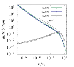
a. b. c.

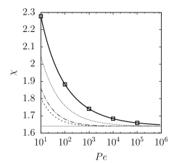
Figure 2: (a) PDFs of (circles) Eulerian flow speed $p_{e}(v)$, (crosses) mean flow speed $p_{m}(v)$ and (squares) flux weighted mean speed distribution $p_{s}(v)$ normalized by the Eulerian mean speed $\langle v_{e}\rangle$ for the Berea sample of Fig. 1. The solid line denotes the power-law $v^{\alpha-1}$ with $\alpha=0.35$. (b) First passage time distribution $\psi_{0}(t|v)$ for local Péclet numbers of (crosses) $Pe_{v}=10^{2}$ (circles) $10$, (squares) $1$ and (diamonds) $10^{-1}$. (c) Tortuosity $\chi$ versus $Pe$ for Gamma-distributed $p_{e}(v)$ with exponents (solid line) $\alpha=0.35$ (dotted) $0.5$, (dash-dotted) $0.8$ and (dashed) $1$. The horizontal line indicates the advective tortuosity $\chi_{a}$.

In order to quantify these mechanisms, we first consider the flow speeds by which particles move along the conducts of length $\ell_{v}$. To this end, we assume that flow within a 3-dimensional conduct of length $\ell_{v}$ can be described by the Poiseuille law, that is, by a parabolic velocity profile. This is a valid approximation because laminar flow in the porous medium is dominated by the drag due to the solid walls. If the diffusion time across is smaller than the advection time along the conduct, a particle samples the velocity profile across the conduct and moves effectively with the average conduct velocity. This is the case for narrow conducts associated with low flow velocities. For wide conducts, diffusion removes particles from the low velocities at the grain walls such that the average particle speed is increased towards the mean. Thus, particle motion along a conduct is dominated by the mean speed $v_{m}$, whose probability density function (PDF) $p_{m}(v)$ is related to the Eulerian speed PDF $p_{e}(v)$ by

$$p_{e}(v)=\int\limits_{0}^{\infty}dv^{\prime}p_{m}(v)\frac{1}{2v^{\prime}}H(2v^{\prime}-v).$$ (2)

The assumption of Poiseuille flow gives a uniform speed PDF in the conduct, such that the Eulerian PDF can be constructed as the weighted sum of the local uniform PDFs represented by the Heaviside function under the integral. The Eulerian PDF $p_{e}(v)$ and thus $p_{m}(v)$ are determined by volumetric sampling of the local flow speeds, while the partitioning of particles at turning points is proportional to the flow rates into the downstream conducts. Thus, the probability $p_{s}(v)$ for a particle to choose the speed $v$ at a turning point is given by the flux-weighted PDF of mean speeds si ,

$$p_{s}(v)=\frac{vp_{m}(v)}{\langle v_{m}\rangle},$$ (3)

where $\langle v_{m}\rangle$ is the network averaged mean velocity. Figure 2a displays the Eulerian $p_{e}(v)$, and $p_{m}(v)$ for the Berea sample, and the corresponding Lagrangian $p_{s}(v)$. The PDF $p_{m}(v)$ of mean speeds is very similar to $p_{e}(v)$ because of the power-law behavior at small velocities. Equations (2)–(3) provide the bridge between Eulerian and Lagrangian flow characteristics. Current approaches that explore mapping the conduct widths to flow speeds via the Poiseuille law and local mass conservation Holzner et al. (2015); De Anna et al. (2017); Alim et al. (2017); Dentz et al. (2018) provide promising avenues to ultimately relate $p_{e}(v)$ to the medium structure, which, however, is beyond the scope of this paper.

Next we consider the impact of diffusion on the PDF of transition times over a single conduct. It is obtained by considering advective-diffusive transport in a $d=1$ dimensional domain of length $\ell_{v}$ characterized by an instantaneous injection at the upstream and an absorbing boundary condition at the downstream end si . The transition time PDF $\psi_{0}(t|v)$ for a single conduct is given by the solute flux over the downstream boundary. It is sharply peaked around the advection time $\tau_{v}=\ell_{v}/v$ for high local Péclet numbers $Pe_{v}=v\ell_{v}/2D$, and broadly distributed with an exponential cutoff at the diffusion time $\tau_{D}$ as illustrated in Figure 2b for $Pe_{v}=10^{2},10,1$ and $10^{-1}$. The mean transition time is given by si

$$\langle\tau|v\rangle=\tau_{v}\frac{Pe_{v}-\exp(-Pe_{v})\sinh(Pe_{v})}{Pe_{v}}.$$ (4)

At high $Pe_{v}$ it tends to the local advection time $\tau_{v}$, at low $Pe_{v}$ to $\tau_{D}/2$. The network-scale PDF $\psi(t)$ of transition times is given in term of $\psi_{0}(t|v)$ and $p_{m}(v)$

$$\psi(t)=\int\limits_{0}^{\infty}dv\frac{vp_{m}(v)}{\langle v_{m}\rangle}\psi_{0}(t|v).$$ (5)

For times $t\ll\tau_{D}$, it can be approximated by $\psi(t)\approx\ell_{v}^{2}t^{-3}p_{m}(\ell_{v}/t)$. For times larger than $\tau_{D}$, $\psi(t)$ decreases to $0$ exponentially fast. Note that this result quantifies particle transition times from first principles, namely pore-scale advection and diffusion, and network scale flow variability.

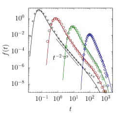
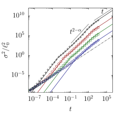
a. b. c.

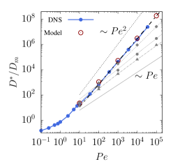
Figure 3: (a) First arrival time PDFs at distance $x\approx 32\ell_{0}$ and (b) $\sigma^{2}(t)$ for (crosses) $Pe=10^{4}$, (circles) $10^{3}$, (squares) $10^{2}$, and (rhombs) $10$. (c) Streamwise hydrodynamic dispersion coefficients versus Péclet number from (full circles) direct numerical simulations, and (empty circles) the model predictions. The gray symbols show the predictions for Gamma-distributed Eulerian speeds with exponents (top to bottom) $\alpha=0.5,0.8,1$, the corresponding lines show the theoretical scalings.

So far, we have considered motion along particle paths while our focus lies on dispersion in streamwise direction, that is, aligned with the mean pressure gradient. In analogy to purely advective motion, the increments $\ell_{v}$ along tortuous particle paths are projected onto the streamwise increments in terms of tortuosity $\chi$ such that the particle position $x(t)$ at time $t$ is given by $x(t)=s(t)/\chi$. In order to determine $\chi$, we note that, under ergodic flow conditions, the asymptotic mean particle velocity is equal to the mean flow velocity $\overline{u}$. This implies that, as particles sample a representative part of the spatial flow variability they assume asymptotically the mean flow velocity, which is equal to the Darcy velocity divided by porosity Bear (1972). The stochastic time-domain random walk (TDRW) model described by Equations (1)–(5) yields for the asymptotic average particle velocity $v_{\infty}=\ell_{v}/\chi\langle\tau\rangle\equiv\overline{u}$, where $\langle\tau\rangle$ is the average transition time Dentz et al. (2004). This gives for tortuosity $\chi=\ell_{v}/\overline{u}\langle\tau\rangle$. Using (5) and (4), we obtain the explicit expression

$$\chi=\chi_{a}\left[1-\int\limits_{0}^{\infty}dv\frac{1-\exp(-Pe_{v})}{Pe_{v}}p_{m}(v)\right]^{-1}.$$ (6)

The behavior of $\chi$ for the Berea sample is shown in Figure 2c. For $Pe\gg 1$ it tends to advective tortuosity $\chi_{a}$ and increases monotonically for decreasing $Pe$.

We use the derived theory to quantify and elucidate anomalous and normal hydrodynamic dispersion behaviors. To this end, we focus on speed PDFs that behave as power-laws for speeds much smaller than the average, $p_{m}(v)\sim v^{\alpha-1}$ with $0<\alpha\leq 1$. Such behaviors have been observed for a wide range of porous media Bijeljic et al. (2013); Puyguiraud et al. (2019b); Souzy et al. (2020). Note that $\alpha=1$ for a channel or tube. For the Berea sample we find $\alpha\approx 0.35$ as shown in Figure 2a. The corresponding transition time PDF behaves as $\psi(t)\sim(t/\tau_{v})^{-2-\alpha}$ for times $t\ll\tau_{D}$, and decays exponentially fast for $t\gg\tau_{D}$, which is a key feature of the impact of pore-scale mixing. To facilitate the analysis, we note that the stochastic TDRW model described by Equations (1)–(6) constitutes a CTRW so that we can use the CTRW machinery to derive the hydrodynamic dispersion behaviors predicted by the theory si .

We focus on the PDF $f(t)$ of first arrival times at a control plane perpendicular to the mean flow direction, and the longitudinal displacement variance $\sigma^{2}(t)=\langle x(t)^{2}\rangle-\langle x(t)\rangle^{2}$. For times $t\ll\tau_{D}$ particles see only the power-law scaling $\psi(t)\sim t^{-2-\alpha}$ of the transition time PDF. In this regime, particle motion is history-dependent because transition times may be of the order of the observation time. CTRW based on the generalized central limit theorem predicts power-law scaling as $f(t)\sim t^{-2-\alpha}$ Berkowitz et al. (2006). The displacement variance is predicted to scale as $\sigma^{2}(t)\sim\overline{u}\ell_{v}(t/\tau_{v})^{2-\alpha}$ for $0<\alpha<1$ and as $\sigma^{2}(t)\sim\overline{u}\ell_{v}(t/\tau_{v})\ln(t/\tau_{v})$ for $\alpha=1$ Shlesinger (1974); si . This means, dispersion is anomalous. For times $t\gg\tau_{D}$ all particles are able to access the full spectrum of transition times and become statistically equal because the memory of the initial velocities is lost. This leads to an exponential cut-off in $f(t)$ Dentz et al. (2004), and linear (Fickian) scaling of $\sigma^{2}(t)$ as $=2D^{\ast}t$. The hydrodynamic dispersion coefficient $D^{\ast}$ can be obtained by matching the preasymptotic and asymptotic expressions for $\sigma^{2}(t)$ at $t=\tau_{D}$. This gives ${D^{\ast}}/{D_{m}}\sim Pe^{2-\alpha}$. A similar behavior was obtained by Bijeljic et al. (2011) based on empirical transition time PDFs using CTRW theory Dentz et al. (2004). The theory presented here directly links these behaviors to the distribution of Eulerian flow speeds. For $\alpha=1$, we obtain ${D^{\ast}}/{D_{m}}\sim Pe\ln(Pe)$, which is equivalent to the one derived by Saffman (1959) and Koch and Brady (1985) based on the assumption that the distribution of flow speeds is flat, which is characteristic of the linear flow profile at pore walls. For $\alpha>1$, the theory predicts $D^{\ast}/D_{m}\sim Pe$. Details are given in the Supplemental Material si .

These features of anomalous and asymptotic Fickian dispersion are illustrated in Figure 3 for the Berea sandstone sample. The power-law scaling and exponential tempering of $f(t)$ are shown in Figure 3a for different $Pe$. Figure 3b shows the evolution of $\sigma^{2}(t)$. The theory predicts the early time ballistic behavior, the cross-over to anomalous dispersion for $t>\tau_{v}$, and the transition to normal dispersion for times $t>\tau_{D}$. The diffusive behavior at very early times $t<D_{m}/\overline{u}^{2}$ is not resolved by the theory because it does not explicitly represent (Brownian) particle motion at short times. The impact of diffusion is accounted for through its effect on particle transition times, tortuosity and velocity sampling as detailed above. The theory predicts that the dependence of $D^{\ast}$ on $Pe$ is constrained between $D^{\ast}/D_{m}\sim Pe^{2}$ and $D^{\ast}/D_{m}\sim Pe$. This is illustrated in Figure 3c, which shows $D^{\ast}$ versus $Pe$ obtained from the Berea sample as well as the theoretical predictions for $\alpha=0.5,0.8,1$ using a Gamma-distributed $p_{e}(v)$.

Data from a broad range of experimental and numerical studies of dispersion in a variety of porous media Pfannkuch (1963); Bear (1972); Bijeljic et al. (2004); Bijeljic and Blunt (2006); Sahimi (2011); Icardi et al. (2014) indicate a non-linear increase of $D^{\ast}$ with $Pe$. These data are often interpreted jointly by a single regression Bear (1972); Sahimi (2011), which implicitly assumes the existence of a universal behavior across different types of porous media. The derived theory indicates that neither the $Pe$-dependence of asymptotic hydrodynamic dispersion nor its evolution are universal, but depend on the flow distribution. On the other hand, the theory shows that dispersion can be predicted based on the distribution of flow speeds, which can be applied across a broad range of porous media.

The derived theory quantifies anomalous and normal hydrodynamic dispersion from first principles in terms of the characteristic velocity scale, the Eulerian flow speed, and pore-scale diffusion. It is valid for $Pe>1$ and based on the knowledge of the Eulerian speed distribution. It is not constrained by transport measurements. The fundamental nature of the considered flow and transport processes in the conceptual picture of a network of conducts allows application of the key elements of the derived theory to transport of dissolved chemicals, bacteria and colloids in a wide range of porous media also under non-Newtonian and multiphase flow conditions.

Appendix A Direct numerical simulations

The numerical flow and transport simulations are performed on the three-dimensional image of a Berea sandstone sample obtained by identifying the connected void phase and the solid phase by processing a X-Ray microtomography image (see for example Gouze et al. (2008) and references therein)

A.1 Flow

In the following we summarize the methodology to solve the flow field. The binary images of the geometry are composed of $300^{3}$ regular voxels (cubes) that represent either void or solid. The mesh used for solving flow is obtain by dividing each of the image voxels by 3 in each of the direction so that 1 voxel of the image is represented by 27 cubic cells of size $\Delta x=\Delta y=\Delta z=1.06\times 10^{-6}$ m. This discretization level is selected such that flow in the smallest throats are is-represented, see also Gjetvaj et al. (2015). Thus, the resulting discretization for the regular grid consists of $900^{3}$ cubic cells. We prescribe pressure boundary conditions at the inlet and outlet, and no-slip conditions at the void-solid interfaces and at the remaining domain boundaries. At the inlet a pressure of $0.1$ Pa in set while it is zero at the outlet. We then solve the flow with the SIMPLE algorithm Patankar (1980) implemented in OpenFOAM Weller et al. (1998). Note that, in order to minimize boundary effects, twenty layers are added at the inlet and outlet Guibert et al. (2015). After convergence, this means, once the residual of the pressure and flow fields between two consecutive steps is below $10^{-5}$, we extract the complete velocity field. Velocity values are given at every interface of the mesh in the normal direction to the face. More details are given in Gjetvaj et al. (2015). The mean flow speed is $7.78\times 10^{-7}$ m/s which corresponds to a Reynolds number of $Re\approx 10^{-5}$, meaning that the flow is laminar and can be described by the Stokes equation. The flow fields used for the simulations at different Péclet numbers are obtained by multiplying this flow field by a constant. The corresponding Reynolds numbers are between $Re\approx 10^{-5}$ for $Pe=1$ and $Re\approx 1$ for $Pe=10^{5}$, which is at the upper limit for which the Stokes assumption is still valid.

A.2 Random walk particle tracking

The random walk particle tracking simulations are based on the Langevin equations

$$\frac{d{\mathbf{x}}(t)}{dt}={\mathbf{v}}[{\mathbf{x}}(t)]+\sqrt{2D}\bm{\xi}(t),$$ (7)

where, $\bm{\xi}=(\xi_{1},\xi_{2},\xi_{3})$ is a Gaussian white noise with zero mean and correlation $\langle\xi_{i}(t)\xi_{j}(t^{\prime})\rangle=\delta(t-t^{\prime})$. We can then discretize the Langevin equations as the current position ${\mathbf{x}}(t)$ plus an advective and a diffusive component as

$${\mathbf{x}}(t+\Delta t)={\mathbf{x}}(t)+{\mathbf{v}}[{\mathbf{x}}(t)]\Delta t+\sqrt{2D\Delta t}\bm{\zeta}(t).$$ (8)

The advective term is based on an extension of the Pollock algorithm (Pollock, 1988; Mostaghimi et al., 2012; Puyguiraud et al., 2019b). Originally, the Pollock algorithm assumes a linear variation of velocity within an the mesh cells in each direction. It is widely used in reservoirs and very high porosity structures. However, this linear interpolation causes precision errors in the vicinity of solid surfaces since a linear interpolation is no longer accurate. This is why Mostaghimi et al. (2012) extended the methodology by introducing different types of quadratic interpolations in the voxels that are in contact with the solid phase. This renders this methodology accurate in low porosity media. This methodology allows to know analytically the position ${\mathbf{x}}(t)$ of a particle for any $t$ and thus permits splitting the trajectory in small time intervals $\Delta t$. The advective and diffusive operators are split on this $\Delta t$ basis, allowing for the computation of the diffusive jumps between advective steps.

The diffusive jumps are computed following the third term on the right side of equation (8) where $\bm{\zeta}=(\zeta_{1},\zeta_{2},\zeta_{3})$ with $\zeta_{i}$ being uniform random variables in $[-\sqrt{3},\sqrt{3}]$ with $\langle\boldsymbol{\zeta}(t)\rangle=\mathbf{0}$ and $\langle\zeta_{i}(t)\zeta_{j}(t)\rangle=\delta_{ij}$. The central limit theorem guarantees that the sum of the random motions is Gaussian. Using uniformly generated random variables rather than Gaussian present two main advantages. The computational cost is reduced and there is a better control on the maximum displacement jump that a particle can do. This avoids unexpectedly large displacement that can jump over solid cells and thus, allows for a moderately large $\Delta t$.

In order to simulate particle displacement over distances larger than the sample size, we reinject the particles at the inlet boundary of the domain once they reach the outlet of the sample. To ensure continuity of the speed series of each particle, we first compute the particle speed $v({\mathbf{x}}_{a})$ at position ${\mathbf{x}}_{a}$ at the outlet. Then, we identify the pore area $\mathcal{A}_{v({\mathbf{x}}_{a})}$ at the inlet plane where the speed values $v({\mathbf{x}}_{b})$ at positions ${\mathbf{x}}_{b}\in\mathcal{A}_{v({\mathbf{x}}_{a})}$ fulfill $v({\mathbf{x}}_{b})\in[v({\mathbf{x}}_{a})-\Delta v,v({\mathbf{x}}_{a})+\Delta v]$, where $\Delta v={v({\mathbf{x}}_{a})}/{200}$. The particle is then reinjected in a random location within $\mathcal{A}_{v_{L}({\mathbf{x}})}$. This procedure preserves the speed continuity and ensures that no artificial decorrelation is occurring. Besides, in the case of a particle exiting the domain through the inlet, by diffusion, the particle is reinjected at the outlet following a similar procedure.

Appendix B Speed distributions

We derive here the distribution of the mean flow speeds and then of the particle speeds that is required in the time-domain random walk approach.

B.1 Mean flow speeds

We conceptualize the porous medium as a network of conducts and joints. Within each conduct, the volumetrically sampled speed distribution is uniform,

$$p(v|v_{m})=\frac{1}{2v_{m}}H(2v_{m}-v),$$ (9)

where $v_{m}$ is the mean speed in the conduct. The Eulerian speed distribution $p_{e}(v)$ is constructed by integration of $p(v|v_{m})$ over all conducts weighted by the distribution $p_{m}(v)$ of mean speeds. This gives

$$p_{e}(2v)=\int\limits_{v}^{\infty}dv_{m}p_{m}(v_{m})\frac{1}{2v_{m}}.$$ (10)

This implies that the distribution of mean pore speeds can be obtained from the Eulerian speed PDF as

$$p_{m}(v)=-2v\frac{dp_{e}(2v)}{dv}.$$ (11)

B.2 Particle speeds

In the time-domain random walk, the partitioning of particles at turning points (the joints) is proportional to the flow rate into the downstream conducts. In our model, the distribution of Eulerian speeds and thus mean speeds is obtained through volumetric sampling within the void space of the porous medium,

$$p_{m}(v)=\frac{1}{V_{0}}\sum_{p}V_{p}\delta(v-v_{p}).$$ (12)

The distribution $p_{s}(v)$ of speeds is weighted by the flow rate of the conducts, which means

$$p_{s}(v)=\frac{1}{\sum_{p}A_{p}v_{p}}\sum_{p}A_{p}v_{p}\delta(v-v_{p}).$$ (13)

We assume that the length of the conducts is approximately constant such that $V_{p}=A_{p}\ell_{0}$. Thus, we can write

$$p_{s}(v)=\frac{1}{\sum_{p}V_{p}v_{p}}\sum_{p}V_{p}v_{p}\delta(v-v_{p})=\frac{v}{\langle v_{e}\rangle}p_{e}(v).$$ (14)

Appendix C Transition time distribution

We first derive the distribution of transition times for a single conduct, and then the compound transition time distribution on the network scale.

C.1 Single Conduct

The transition time distribution for a single conduct is obtained from the solution of the following first-passage problem. We consider an instantaneous injection of tracer at the upstream turning point at $x=0$, and an absorbing boundary at the downstream turning point at $x=\ell_{v}$. This means

$$\frac{\partial g(x,t)}{\partial t}+v\frac{\partial g(x,t)}{\partial x}-D\frac{\partial^{2}g(x,t)}{\partial x^{2}}=0$$ (15)

with the boundary conditions

$$vg(x,t)-D\frac{g(x,t)}{\partial x}=\delta(t), x=0,$$ (16)

$$g(x,t)=0, x=\ell_{v},$$ (17)

and the initial condition $g(x,t=0)=0$. The first passage time distribution over the downstream boundary is given by

$$\psi_{0}(t|v)=-\left.D\frac{\partial g(x,t)}{\partial x}\right|_{x=\ell_{v}}.$$ (18)

We solve this first passage problem in Laplace space. Laplace transform of (15) gives

$$\lambda g^{\ast}(x,\lambda)+v\frac{\partial g^{\ast}(x,\lambda)}{\partial x}-D\frac{\partial^{2}g^{\ast}(x,\lambda)}{\partial x^{2}}=0.$$ (19)

The solution is given by

$$g^{\ast}(x,\lambda)=A(\lambda)\exp(Pe_{v}x/\ell_{v})\sinh\left[\frac{\ell_{v}-x}{\ell_{v}}B(\lambda)\right], B(\lambda)=\sqrt{Pe_{v}^{2}+\lambda\tau_{D}},$$ (20)

where we defined $Pe_{v}=v\ell_{v}/2D$. The constant $A(\lambda)$ is determined from the boundary condition at $0$,

$$vg^{\ast}(x,\lambda)-D\frac{g^{\ast}(x,\lambda)}{\partial x}=1, x=0.$$ (21)

Inserting (20) into the latter gives

$$A=\frac{\ell_{v}/D}{Pe_{v}\sinh(B)+B\cosh(B)}.$$ (22)

Thus, we obtain $g^{\ast}(x,\lambda)$

$$g^{\ast}(x,\lambda)=\frac{\ell_{v}}{D}\frac{\exp(Pe_{v}x/\ell_{v})\sinh\left[\frac{\ell_{v}-x}{\ell_{v}}B(\lambda)\right]}{Pe_{v}\sinh(B)+B\cosh(B)}.$$ (23)

This gives for the first passage time distribution

$$\psi_{0}^{\ast}(\lambda|v)=\frac{B\exp(Pe_{v})}{Pe_{v}\sinh(B)+B\cosh(B)}.$$ (24)

C.1.1 Moments

The mean travel time is defined by

$$\langle\tau|v\rangle=-\left.\frac{df^{\ast}(\lambda)}{d\lambda}\right|_{\lambda=0}.$$ (25)

We obtain

$$\langle\tau|v\rangle =\tau_{v}\left[1-\frac{\exp(-Pe_{v})\sinh(Pe_{v})}{Pe_{v}}\right],$$ (26)

where we defined $\tau_{v}=\ell_{v}/v$. The mean squared travel time is defined by

$$\langle\tau^{2}|v\rangle=\left.\frac{d^{2}f^{\ast}(\lambda)}{d\lambda^{2}}\right|_{\lambda=0}.$$ (27)

We obtain

$$\langle\tau^{2}|v\rangle=\tau_{v}^{2}\left(1-\frac{1}{Pe_{v}^{2}}+\frac{\exp(-2Pe_{v})}{Pe_{v}}\left[3+\frac{1}{2Pe_{v}}+\frac{\exp(-2Pe_{v})}{2Pe_{v}}\right]\right).$$ (28)

Figure 4: First passage time distribution $\psi_{0}(t|v)$ obtained from numerical inverse Laplace transform of (24) for local Péclet numbers of (crosses) $Pe_{v}=10^{2}$ (circles) $10$, (squares) $1$ and (diamonds) $10^{-1}$. The solid lines denote the corresponding approximations by the truncated inverse Gaussian distribution (29).

C.1.2 Numerical Approximation

Numerically, we approximate $\psi_{0}(t|v)$ by the truncated inverse Gaussian distribution

$$G(t)=\frac{\exp\left[-\frac{\tau_{v}^{-2}(t-\tau_{v})^{2}}{4t/\tau_{D}}\right]}{t\sqrt{4\pi t/\tau_{D}}}\exp(-kt-Pe_{v}+\sqrt{Pe_{v}^{2}+k\tau_{D}}).$$ (29)

The constant $k$ is chosen such that $G(t)$ has the same mean transition time as $\psi_{0}(t|v)$. It is determined as follows. The Laplace transform of $G(t)$ is given by

$$G^{\ast}(\lambda)=\exp\left[-\sqrt{Pe_{v}^{2}+(\lambda+k)\tau_{D}}+\sqrt{Pe_{v}^{2}+k\tau_{D}}\right].$$ (30)

The first moment is given by

$$m_{G}=\frac{\tau_{D}}{2\sqrt{Pe_{v}^{2}+k\tau_{D}}}\equiv\langle\tau|v\rangle.$$ (31)

Thus, we obtain for $k$

$$k\tau_{D}=\frac{\tau_{D}^{2}}{4\langle\tau|v\rangle^{2}}-Pe_{v}^{2}=Pe_{v}^{2}\left(\frac{\tau_{v}^{2}}{\langle\tau|v\rangle^{2}}-1\right).$$ (32)

Figure 4 shows the first passage time distribution and the approximation by the truncated inverse Gaussian distribution. Random numbers are sampled numerically from the truncated inverse Gaussian distribution by using the algorithm of Michael et al. (1976) for the inverse Gaussian random variable in combination with rejection sampling in order to account for the exponential cutoff.

C.2 Network scale

We first analyze the behavior of the transition time distribution and specifically its behavior for times smaller and larger than $\tau_{D}$. Then, we consider the behavior of the mean and of the mean squared travel time for large Péclet numbers.

The transition time distribution $\psi(t)$ for the network of conducts is obtained for $\psi_{0}(t|v)$ and $p_{m}(v)$ as

$$\psi(t)=\int\limits_{0}^{\infty}dv\frac{v}{\langle v_{m}\rangle}p_{m}(v)\psi_{0}(t|v).$$ (33)

For $Pe_{v}\gg 1$, that is for $v\gg D_{m}/\ell_{v}$ $\psi_{0}(t|v)$ is sharply peaked about $\tau_{v}=\ell_{v}/v$, while for $Pe_{v}\ll 1$, that it $v\ll D_{m}/\ell_{v}$ it is $\psi_{0}(t|v)=\psi_{0}(t)$ independent of $v$ and a function of $\tau_{D}$ only. Thus, we can approximate

$$\psi(t)\approx\int\limits_{D_{m}/\ell_{v}}^{\infty}dv\frac{v}{\langle v_{m}\rangle}p_{m}(v)\delta(t-\ell_{v}/v)+\int\limits_{0}^{D_{m}/\ell_{v}}dv\frac{v}{\langle v_{m}\rangle}p_{m}(v)\psi_{0}(t).$$ (34)

This gives

$$\psi(t)\approx\frac{\ell_{v}}{\langle v_{m}\rangle t^{3}}p_{m}(\ell_{v}/t)H(\tau_{D}-t)+C\psi_{0}(t),$$ (35)

with $C$ a constant. Thus, for times $t\ll\tau_{D}$, the transition time distribution is dominated by the speed distribution $p_{m}(v)$, and for time $t\gg\tau_{D}$ by the diffusive cut-off $\tau_{D}$.

In the following, we consider speed distributions that behave as the power-law

$$p_{m}(v)\sim v^{-1-\alpha}$$ (36)

for $v\ll v_{0}$ with $v_{0}$ a characteristic velocity, and which decay exponentially fast for $v\gg v_{0}$. For illustration one can think of a Gamma distribution. The transition time distribution thus behaves as

$$\psi(t)\sim t^{-2-\alpha}$$ (37)

for $t\ll\tau_{D}$.

The mean travel time is given by

$$\langle\tau\rangle =\int\limits_{0}^{\infty}dv\frac{v}{\langle v_{m}\rangle}p_{m}(v)\langle\tau|v\rangle.$$ (38)

Inserting expression (26) gives

$$\langle\tau\rangle =\tau_{v}\left[1-\int\limits_{0}^{\infty}dvp_{m}(v)\frac{\exp(-Pe_{v})\sinh(Pe_{v})}{Pe_{v}}\right].$$ (39)

Next, we rescale the integration variable as $v\to v/v_{m}$, which gives

$$\langle\tau\rangle=\tau_{v}\left[1-\int\limits_{0}^{\infty}dv\hat{p}_{m}(v)\frac{\exp(-Pe_{c}v)\sinh(Pe_{c}v)}{Pe_{c}v}\right],$$ (40)

where we defined $Pe_{c}=\langle v_{m}\rangle\ell_{v}/2D_{m}$ and $\hat{p}_{m}(v)=\langle v_{m}\rangle p_{m}(\langle v_{m}\rangle v)$. Note that $Pe_{c}=Pe\ell_{v}/\ell_{0}$. The leading order behavior of $\langle\tau\rangle$ for $Pe_{c}\gg 1$ is

$$\langle\tau\rangle=\tau_{v}+\dots,$$ (41)

where the dots denote contributions of order $Pe$.

The mean squared travel time is

$$\langle\tau^{2}\rangle =\int\limits_{0}^{\infty}dv\frac{v}{\langle v_{m}\rangle}\tau_{v}^{2}p_{m}(v)F(Pe_{v})=\int\limits_{0}^{\infty}dv\frac{\ell_{v}^{2}}{v\langle v_{m}\rangle}p_{m}(v)F(Pe_{v})=\tau_{v}^{2}\int\limits_{0}^{\infty}dv\frac{\langle v_{m}\rangle}{v}p_{m}(v)F(Pe_{v}),$$ (42)

where we defined $\langle\tau^{2}|v\rangle=\tau_{v}^{2}F(Pe_{v})$. We note that $F(Pe_{v})$ behaves for $Pe_{v}\ll 1$ as $F(Pe_{v})=5Pe_{v}^{2}/3$ and is equal to $1$ in the limit $Pe_{v}\to\infty$. Next, we rescale the integration variable as $v\to v/v_{m}$. This gives

$$\langle\tau^{2}\rangle =\tau_{v}^{2}\int\limits_{0}^{\infty}dv\frac{1}{v}\hat{p}_{m}(v)F(vPe_{c}).$$ (43)

The mean of $\hat{p}_{m}(v)$ is equal to $1$. If

$$\int\limits_{0}^{\infty}dvv^{-1}\hat{p}_{m}(v)<\infty,$$ (44)

this means if $\hat{p}_{m}(v)$ goes to $0$ for $v\to 0$, the mean squared transition time behaves as

$$\langle\tau^{2}\rangle\sim\tau_{v}^{2}$$ (45)

in leading order for $Pe_{c}\gg 1$. If $\hat{p}_{m}(v)$ has an integrable singularity at $0$, this means, if $\hat{p}_{m}(v)\sim v^{\alpha-1}$ with $0<\alpha\leq 1$, we rescale the integration variable as $v\to vPe_{c}$. This gives

$$\langle\tau^{2}\rangle =\tau_{v}^{2}\int\limits_{0}^{\infty}dv\frac{1}{v}\hat{p}_{m}(v/Pe_{c})F(v).$$ (46)

We set $\hat{p}_{m}(v)=v^{\alpha-1}\varphi(v)$, where $\varphi(v)$ goes toward a constant for $v\to 0$ and decays exponentially fast for $v\to\infty$. For illustration, one may think of a Gamma distribution with mean $1$. Thus, we obtain

$$\langle\tau^{2}\rangle =\tau_{v}^{2}Pe_{c}^{1-\alpha}\int\limits_{0}^{\infty}dvv^{\alpha-2}\varphi(v/Pe_{c})F(v).$$ (47)

For $0<\alpha<1$, the leading order behavior in the limit of large $Pe_{c}\gg 1$ is

$$\langle\tau^{2}\rangle \sim\tau_{v}^{2}Pe_{c}^{1-\alpha}.$$ (48)

For $\alpha=1$, we can write

$$\langle\tau^{2}\rangle =\tau_{v}^{2}\int\limits_{0}^{\infty}dv\frac{1}{v}\varphi(v/Pe_{c})F(v)\approx\tau_{v}^{2}\int\limits_{0}^{Pe_{v}}dv\frac{1}{v}F(v),$$ (49)

because $\varphi(v/Pe_{c})$ sets a cutoff at $Pe_{c}$. Since $F(v)\to 1$ for $v\gg 1$, we obtain in leading order

$$\langle\tau^{2}\rangle =\tau_{v}^{2}\ln(Pe_{c}).$$ (50)

Appendix D Implementation of the stochastic time-domain random walk model

The numerical simulations of the derived stochastic particle model is based on the equations of motion

$$x_{n+1}=x_{n}+\ell_{v}/\chi, t_{n+1}=t_{n}+\tau_{n}.$$ (51)

The time increments $\tau_{n}$ are generated as follows. A speed $v$ is sampled according to the distribution $p_{s}(v)$ by inverse sampling. Then, the transition time is obtained by sampling from $\psi_{0}(t|v)$ approximated by the truncated inverse Gaussian distribution (29).

The displacement variance is determined as

$$\sigma^{2}(t)=\langle x_{n_{t}}^{2}\rangle-\langle x_{n_{t}}\rangle^{2},$$ (52)

where $n_{t}=\max(n|t_{n}\leq t)$. The first passage time distributions are determined as

$$t_{a}=\sum\limits_{n=1}^{n_{c}-1}\tau_{n}+\tau_{n_{c}}\frac{x\chi-s_{n}}{\ell_{v}},$$ (53)

where $n_{c}=\lceil\chi x/\ell_{v}\rceil$. The interpolation for the last step is negligible for $n_{c}\gg 1$.

Appendix E Continuous time random walks

The continuous time random walk framework Scher and Lax (1973); Berkowitz et al. (2006) gives for the evolution equation of the particle distribution $p(x,t)$ in the derived stochastic time-domain random walk model, the following set of equations,

$$p(x,t) =\int\limits_{0}^{t}dt^{\prime}R(x,t^{\prime})\int\limits_{t-t^{\prime}}^{\infty}dt^{\prime\prime}\psi(t^{\prime\prime}),$$ (54)

$$R(x,t) =\delta(x)\delta(t)+\int\limits_{0}^{t}dtR(x-\ell_{v}/\chi,t^{\prime})\psi(t-t^{\prime}).$$ (55)

These equations can be solved for the Fourier-Laplace transform $\tilde{p}^{\ast}(k,\lambda)$ of $p(x,t)$ Shlesinger (1974), which gives

$$\tilde{p}^{\ast}(x,\lambda)=\frac{1}{\lambda}\frac{1-\psi^{\ast}(\lambda)}{1-\exp(ik\ell_{v}/\chi)\psi^{\ast}(\lambda)}.$$ (56)

The Fourier transform is defined here as

$$\tilde{\varphi}(k)=\int\limits_{-\infty}^{\infty}dx\exp(ikx)\varphi(x), \varphi(x)=\int\limits_{-\infty}^{\infty}\frac{dk}{2\pi}\exp(-ikx)\tilde{\varphi}(k).$$ (57)

The first and second displacement moments are defined in terms of $\tilde{p}^{\ast}(k,\lambda)$ as

$$m^{\ast}_{1}(\lambda) =-i\left.\frac{\partial\tilde{p}^{\ast}(k,\lambda)}{\partial k}\right|_{k=0}$$ (58)

$$m^{\ast}_{2}(\lambda) =-\left.\frac{\partial^{2}\tilde{p}^{\ast}(k,\lambda)}{\partial k^{2}}\right|_{k=0}.$$ (59)

Using expression (56), we obtain Shlesinger (1974)

$$m_{1}^{\ast}(\lambda) =v_{0}\lambda^{-2}\mathcal{K}^{\ast}(\lambda),$$ (60a)

$$m_{2}^{\ast}(\lambda) =2D_{0}\lambda^{-2}\mathcal{K}^{\ast}(\lambda)+2v_{0}^{2}\lambda^{-3}\mathcal{K}^{\ast}(\lambda)^{2},$$ (60b)

where we defined

$$\mathcal{K}^{\ast}(\lambda)=\frac{\langle\tau\rangle\lambda\psi^{\ast}(\lambda)}{1-\psi^{\ast}(\lambda)},$$ (61)

and

$$v_{0}=\frac{\ell_{v}}{\chi\langle\tau\rangle}, D_{0}=\frac{\ell_{v}^{2}}{2\chi^{2}\langle\tau\rangle}.$$ (62)

E.1 Asymptotic transport

In order to determine the asymptotic large scale transport properties, we expand the kernel (61) up to linear order in $\lambda$

$$\mathcal{K}^{\ast}(\lambda)=1+\lambda\mathcal{K}^{\infty}, \mathcal{K}^{\infty}=\frac{1}{2}\frac{\langle\tau^{2}\rangle-2\langle\tau\rangle^{2}}{\langle\tau\rangle}.$$ (63)

Thus, we obtain for (60)

$$m_{1}^{\ast}(\lambda) =v_{0}\lambda^{-2}(1+\lambda\mathcal{K}^{\infty}),$$ (64)

$$m_{2}^{\ast}(\lambda) =2D_{0}\lambda^{-2}(1+\lambda\mathcal{K}^{\infty})+2v_{0}^{2}\lambda^{-3}(1+\lambda\mathcal{K}^{\infty})^{2}.$$ (65)

Inverse Laplace transform gives

$$m_{1}(t) =v_{0}(t+\mathcal{K}^{\infty})$$ (66a)

$$m_{2}(t) =2D_{0}(t+\mathcal{K}^{\infty})+v_{0}^{2}(t+\mathcal{K}^{\infty})^{2}+2v_{0}^{2}\mathcal{K}^{\infty}t+{\mathcal{K}^{\infty}}^{2}.$$ (66b)

The mean velocity and hydrodynamic dispersion coefficient are defined by

$$v_{\infty} =\frac{d}{dt}m_{1}(t)$$ (67)

$$D^{\ast} =\frac{1}{2}\frac{d}{dt}\left[m_{2}(t)-m_{1}(t)^{2}\right].$$ (68)

Using (66), we obtain

$$v_{\infty} =v_{0}$$ (69)

$$D^{\ast} =D_{0}+v_{0}^{2}\frac{1}{2}\frac{\langle\tau^{2}\rangle-2\langle\tau\rangle^{2}}{\langle\tau\rangle}=D_{0}\left(1+\frac{\langle\tau^{2}\rangle-2\langle\tau\rangle^{2}}{\langle\tau\rangle^{2}}\right)=D_{0}\frac{\sigma_{\tau}^{2}}{\langle\tau\rangle^{2}}.$$ (70)

E.1.1 Tortuosity

The macroscopic transport velocity is equal to the mean pore velocity $v_{\infty}=\overline{u}$ Bear (1972). Thus, we obtain from (69) with (62) that the tortuosity is given by

$$\chi=\frac{\ell_{v}}{\overline{u}\langle\tau\rangle}.$$ (71)

Using (39) gives the explicit expression

$$\chi=\chi_{a}\left[1-\int\limits_{0}^{\infty}dvp_{m}(v)\frac{\exp(-Pe_{v})\sinh(Pe_{v})}{Pe_{v}}\right]^{-1},$$ (72)

where $\chi_{a}=\langle v_{e}\rangle/\overline{u}$.

E.1.2 Hydrodynamic dispersion coefficient

Equation (71) together with (62) in (70) gives for the hydrodynamic dispersion coefficient

$$D^{\ast}=\overline{u}^{2}\frac{\sigma_{\tau}^{2}}{2\langle\tau\rangle}.$$ (73)

The full Péclet dependence of $D^{\ast}$ can be obtained by using expressions (39) and (42) for the mean and mean squared transition times.

We determine now the leading order behavior of $D^{\ast}$ for $Pe_{c}\gg 1$. For $0<\alpha<1$, we obtain by using (41) and (48)

$$D^{\ast}\sim\overline{u}^{2}\tau_{v}Pe_{c}^{1-\alpha}=\langle v_{m}\rangle\ell_{v}\chi_{a}^{-2},Pe_{c}^{1-\alpha}$$ (74)

and therefore

$$D^{\ast}/D_{m}\sim Pe_{c}^{2-\alpha}.$$ (75)

Similarly, we obtain for $\alpha=1$ by using (50)

$$D^{\ast}\sim\overline{u}^{2}\tau_{v}\ln(Pe_{c})=\langle v_{m}\rangle\ell_{v}\chi_{a}^{-2}\ln(Pe_{c}),$$ (76)

and thus

$$D^{\ast}/D_{m}\sim Pe_{c}\ln(Pe_{c}).$$ (77)

For $\alpha>1$, we obtain by using (45)

$$D^{\ast}\sim\overline{u}^{2}\tau_{v}=\langle v_{m}\rangle\ell_{v}\chi_{a}^{-2},$$ (78)

and thus

$$D^{\ast}/D_{m}\sim Pe_{c}.$$ (79)

E.2 Anomalous dispersion

Anomalous dispersion is measured by the displacement variance $\sigma^{2}(t)=m_{2}(t)-m_{1}(t)$. The first and second displacement moments $m_{1}(t)$ and $m_{2}(t)$ are given in Laplace space by (60). At times $t\ll\tau_{D}$, the transition time distribution behaves as $\psi(t)\sim t^{-2-\alpha}$. For $0<\alpha<1$, its Laplace transform can be expanded as

$$\psi^{\ast}(\lambda)=1-\lambda\langle\tau\rangle+b\lambda^{1+\alpha},$$ (80)

with $b$ a constant. Inserting this expansion into (61), we obtain in leading order for $\mathcal{K}(\lambda)$

$$\mathcal{K}(\lambda)=1+b\lambda^{\alpha}/\langle\tau\rangle.$$ (81)

Thus, we obtain for $m_{1}^{\ast}(\lambda)$

$$m_{1}^{\ast}(\lambda)=v_{0}\lambda^{-2}+b\lambda^{\alpha-2}/\langle\tau\rangle$$ (82)

This implies

$$m_{1}(t)=v_{0}t+\dots,$$ (83)

where the dots denote subleading contributions of order $t^{1-\alpha}$. For the second moment, we obtain

$$m_{2}^{\ast}(\lambda)=2D_{0}\lambda^{-2}+2v_{0}^{2}\lambda^{-3}+2bv_{0}^{2}\lambda^{\alpha-3}/\langle\tau\rangle,$$ (84)

Inverse Laplace transform gives

$$m_{2}(t)=2D_{0}t+v_{0}^{2}t^{2}+2v_{0}^{2}bt^{2-\alpha}/\langle\tau\rangle\Gamma(1-\alpha).$$ (85)

Thus, we obtain for the displacement variance

$$\sigma^{2}(t)\sim t^{2-\alpha}.$$ (86)

For $\alpha=1$, the Laplace transform of $\psi(t)$ can be expanded as

$$\psi^{\ast}(\lambda)=1-\langle\tau\rangle\lambda-c\lambda^{2}\ln(\lambda),$$ (87)

with $c$ a constant. Inserting this expansion into (61), we obtain in leading order for $\mathcal{K}(\lambda)$

$$\mathcal{K}(\lambda)=1-c\lambda\ln(\lambda)/\langle\tau\rangle.$$ (88)

Thus, we obtain for $m_{1}^{\ast}(\lambda)$

$$m_{1}^{\ast}(\lambda)=v_{0}\lambda^{-2}+\dots$$ (89)

This implies

$$m_{1}(t)=v_{0}t+\dots,$$ (90)

where the dots denote subleading contributions. For the second moment, we obtain

$$m_{2}^{\ast}(\lambda)=2D_{0}\lambda^{-2}+2v_{0}^{2}\lambda^{-3}-2v_{0}^{2}c\lambda^{-2}\ln(\lambda)/\langle\tau\rangle.$$ (91)

Inverse Laplace transform gives

$$m_{2}(t)=2D_{0}t+v_{0}^{2}t^{2}+2v_{0}^{2}c^{\prime}t\ln(t)/\langle\tau\rangle,$$ (92)

with $c^{\prime}$ a constant. Thus, we obtain for the displacement variance

$$\sigma^{2}(t)\sim t\ln(t).$$ (93)

References

- Brenner and Edwards (1993) H. Brenner and D. Edwards, Macrotransport Processes (Butterworth-Heinemann, MA, USA, 1993).
- Sahimi (2011) M. Sahimi, Flow and transport in porous media and fractured rock: from classical methods to modern approaches (John Wiley & Sons, 2011).
- Valocchi et al. (2018) A. J. Valocchi, D. Bolster, and C. J. Werth, Transport in Porous Media 130, 157 (2018).
- Niemi et al. (2017) A. Niemi, J. Bear, and J. Bensabat, eds., Geological Storage of CO2 in Deep Saline Formations (Springer Netherlands, 2017).
- Maggiolo et al. (2020) D. Maggiolo, F. Picano, F. Zanini, S. Carmignato, M. Guarnieri, S. Sasic, and H. Ström, Journal of Fluid Mechanics 896 (2020), 10.1017/jfm.2020.344.
- Berg et al. (2019) M. Berg, Y. Davit, M. Quintard, and S. Lorthois, Journal of Fluid Mechanics 884 (2019), 10.1017/jfm.2019.866.
- de Josselin de Jong (1958) G. de Josselin de Jong, Trans. Amer. Geophys. Un. 39, 67 (1958).
- Saffman (1959) P. G. Saffman, Journal of Fluid Mechanics 6, 321 (1959).
- Bear (1972) J. Bear, Dynamics of fluids in porous media (American Elsevier, New York, 1972).
- Isichenko (1992) M. B. Isichenko, Reviews of Modern Physics 64, 961 (1992).
- Bouchaud and Georges (1990) J. P. Bouchaud and A. Georges, Phys. Rep. 195, 127 (1990).
- Moroni and Cushman (2001) M. Moroni and J. H. Cushman, Physics of Fluids 13, 81 (2001).
- Levy and Berkowitz (2003) M. Levy and B. Berkowitz, Journal of contaminant hydrology 64, 203 (2003).
- Seymour et al. (2004) J. D. Seymour, J. P. Gage, S. L. Codd, and R. Gerlach, Physical Review Letters 93 (2004), 10.1103/physrevlett.93.198103.
- Morales et al. (2017) V. L. Morales, M. Dentz, M. Willmann, and M. Holzner, Geophysical Research Letters 44, 9361 (2017).
- Carrel et al. (2018) M. Carrel, V. L. Morales, M. Dentz, N. Derlon, E. Morgenroth, and M. Holzner, Water resources research 54, 2183 (2018).
- Souzy et al. (2020) M. Souzy, H. Lhuissier, Y. Méheust, T. L. Borgne, and B. Metzger, Journal of Fluid Mechanics 891 (2020), 10.1017/jfm.2020.113.
- Gouze et al. (2008) P. Gouze, T. Le Borgne, R. Leprovost, G. Lods, T. Poidras, and P. Pezard, Water Resources Research 44 (2008).
- Haggerty and Gorelick (1995) R. Haggerty and S. M. Gorelick, Water Resources Research 31, 2383 (1995).
- Bijeljic et al. (2011) B. Bijeljic, P. Mostaghimi, and M. J. Blunt, Phys. Rev. Lett. 107, 204502 (2011).
- Bijeljic et al. (2013) B. Bijeljic, A. Raeini, P. Mostaghimi, and M. J. Blunt, Physical Review E 87 (2013), 10.1103/physreve.87.013011.
- De Anna et al. (2013) P. De Anna, T. Le Borgne, M. Dentz, A. M. Tartakovsky, D. Bolster, and P. Davy, Physical review letters 110, 184502 (2013).
- Icardi et al. (2014) M. Icardi, G. Boccardo, D. L. Marchisio, T. Tosco, and R. Sethi, Physical Review E 90, 013032 (2014).
- Kang et al. (2014) P. K. Kang, P. de Anna, J. P. Nunes, B. Bijeljic, M. J. Blunt, and R. Juanes, Geophysical Research Letters 41, 6184 (2014).
- Meyer and Bijeljic (2016) D. W. Meyer and B. Bijeljic, Physical Review E 94, 013107 (2016).
- Li et al. (2018) M. Li, T. Qi, Y. Bernabé, J. Zhao, Y. Wang, D. Wang, and Z. Wang, Scientific Reports 8 (2018), 10.1038/s41598-018-22224-w.
- Liu and Kitanidis (2012) Y. Liu and P. K. Kitanidis, Groundwater 50, 927 (2012).
- Dentz et al. (2018) M. Dentz, M. Icardi, and J. J. Hidalgo, Journal of Fluid Mechanics 841, 851 (2018).
- Puyguiraud et al. (2019a) A. Puyguiraud, P. Gouze, and M. Dentz, Transport in Porous Media 128, 837 (2019a).
- Nissan and Berkowitz (2019) A. Nissan and B. Berkowitz, Physical Review E 99 (2019), 10.1103/physreve.99.033108.
- Koch and Brady (1985) D. L. Koch and J. F. Brady, Journal of Fluid Mechanics 154, 399 (1985).
- Scheven (2013) U. M. Scheven, Physical Review Letters 110 (2013), 10.1103/physrevlett.110.214504.
- Bijeljic and Blunt (2006) B. Bijeljic and M. J. Blunt, Water Resources Research 42 (2006), 10.1029/2005WR004578.
- (34) See Supplemental Material at [URL inserted by publisher] for the setup of the direct numerical simulations, and detailed derivations, which includes Refs. [35-43].
- Gouze et al. (2008) P. Gouze, Y. Melean, T. Le Borgne, M. Dentz, and J. Carrera, Water Resources Research 44 (2008), 10.1029/2007WR006690.
- Gjetvaj et al. (2015) F. Gjetvaj, A. Russian, P. Gouze, and M. Dentz, Water Resources Research 51, 8273 (2015).
- Patankar (1980) S. V. Patankar, Numerical Heat Transfer and Fluid Flow (Hemisphere Publishing Corporation, 1980).
- Weller et al. (1998) H. G. Weller, G. Tabor, H. Jasak, and C. Fureby, Computers in physics 12, 620 (1998).
- Guibert et al. (2015) R. Guibert, P. Horgue, G. Debenest, and M. Quintard, Mathematical Geosciences , 1 (2015).
- Pollock (1988) D. W. Pollock, Ground Water 26, 743 (1988).
- Mostaghimi et al. (2012) P. Mostaghimi, B. Bijeljic, and M. Blunt, Mathematical Geosciences , 1131 (2012).
- Michael et al. (1976) J. R. Michael, W. R. Schucany, and R. W. Haas, The American Statistician 30, 88 (1976).
- Scher and Lax (1973) H. Scher and M. Lax, Phys. Rev. B 7, 4491 (1973).
- Puyguiraud et al. (2019b) A. Puyguiraud, P. Gouze, and M. Dentz, Water Resources Research 55 (2019b), 10.1029/2018WR023702.
- Koponen et al. (1996) A. Koponen, M. Kataja, and J. Timonen, Phys. Rev. E 54, 406 (1996).
- Ghanbarian et al. (2013) B. Ghanbarian, A. G. Hunt, R. P. Ewing, and M. Sahimi, Soil Science Society of America Journal 77, 1461 (2013).
- Holzner et al. (2015) M. Holzner, V. L. Morales, M. Willmann, and M. Dentz, Physical Review E 92, 013015 (2015).
- De Anna et al. (2017) P. De Anna, B. Quaife, G. Biros, and R. Juanes, Phys. Rev. Fluids 2, 124103 (2017).
- Alim et al. (2017) K. Alim, S. Parsa, D. A. Weitz, and M. P. Brenner, Physical Review Letters 119 (2017), 10.1103/physrevlett.119.144501.
- Dentz et al. (2004) M. Dentz, A. Cortis, H. Scher, and B. Berkowitz, Adv. Water Resour. 27, 155 (2004).
- Berkowitz et al. (2006) B. Berkowitz, A. Cortis, M. Dentz, and H. Scher, Reviews of Geophysics 44 (2006).
- Shlesinger (1974) M. F. Shlesinger, Journal of Statistical Physics 10, 421 (1974).
- Pfannkuch (1963) H. O. Pfannkuch, Rev. Inst. Fr. Petr. 18, 215 (1963).
- Bijeljic et al. (2004) B. Bijeljic, A. H. Muggeridge, and M. J. Blunt, Water Resources Research 40 (2004).