Analytical representation of the Local Field Correction of the Uniform Electron Gas within the Effective Static Approximation

Abstract

The description of electronic exchange–correlation effects is of paramount importance for many applications in physics, chemistry, and beyond. In a recent Letter, Dornheim et al. [Phys. Rev. Lett. 125, 235001 (2020)] have presented the effective static approximation (ESA) to the local field correction (LFC), which allows for the highly accurate estimation of electronic properties such as the interaction energy and the static structure factor. In the present work, we give an analytical parametrization of the LFC within ESA that is valid for any wave number, and available for the entire range of densities ($0.7\leq r_{s}\leq 20$) and temperatures ($0\leq\theta\leq 4$) that are relevant for applications both in the ground state and in the warm dense matter regime. A short implementation in Python is provided, which can easily be incorporated into existing codes.

In addition, we present an extensive analysis of the performance of ESA regarding the estimation of various quantities like the dynamic structure factor, static dielectric function, the electronically screened ion-potential, and also stopping power in electronic medium. In summary, we find that the ESA gives an excellent description of all these quantities in the warm dense matter regime, and only becomes inaccurate when the electrons start to form a strongly correlated electron liquid ($r_{s}\sim 20$). Moreover, we note that the exact incorporation of exact asymptotic limits often leads to a superior accuracy compared to the neural-net representation of the static LFC [J. Chem. Phys. 151, 194104 (2019)].

I Introduction

The accurate description of many-electron systems is of paramount importance for many applications in physics, quantum chemistry, material science, and related disciplines Giuliani and Vignale (2008); Foulkes et al. (2001). In this regard, the uniform electron gas (UEG) Loos and Gill (2016); Dornheim et al. (2018a), which is comprised of correlated electrons in a homogeneous, neutralizing positive background (also known as ”jellium” or quantum one-component plasma), constitutes a fundamental model system. Indeed, our improved understanding of the UEG has facilitated many key insights like the quasi-particle picture of collective excitations Bohm and D. Pines (1952) and the Bardeen-Cooper-Schrieffer theory of superconductivity Bardeen et al. (1957).

In the ground state, many properties of the UEG have been accurately determined on the basis of quantum Monte Carlo (QMC) simulations Ceperley (1978); Ceperley and Alder (1980); Bowen et al. (1994); Moroni et al. (1992, 1995); Ortiz and Ballone (1994); Ortiz et al. (1999); Zong et al. (2002); Shepherd et al. (2012a, b); Spink et al. (2013); Drummond et al. (2004); Fraser et al. (1996), which have subsequently been used as input for various parametrizations Perdew and Zunger (1981); Perdew and Wang (1992a, b); Vosko et al. (1980); Gori-Giorgi et al. (2000); Corradini et al. (1998); Takada (2016). These, in turn, have provided the basis of the possibly unrivaled success of density functional theory (DFT) regarding the description of real materials Perdew et al. (1996); Burke (2012); Jones (2015).

Over the last decade or so, there has emerged a remarkable interest in warm dense matter (WDM)–an exotic state with high temperatures and extreme densities. In nature, these conditions occur in various astrophysical objects such as giant planet interiors Saumon et al. (1992); Militzer et al. (2008); Guillot et al. (2018), brown dwarfs Becker et al. (2014); Saumon et al. (1992), and neutron star crusts Daligault and Gupta (2009). On earth, WDM has been predicted to occur on the pathway towards inertial confinement fusion Hu et al. (2011), and is relevant for the new field of hot-electron chemistry Brongersma et al. (2015); Mukherjee et al. (2013).

Consequently, WDM is nowadays routinely realized in large research facilities around the globe; see Ref. Falk (2018) for a recent review of different experimental techniques. Further, we mention that there have been many remarkable experimental discoveries in this field, such as the observation of diamond formation by Kraus et al. Kraus et al. (2016, 2017), or the measurement of plasmons in aluminum by Sperling et al. Sperling et al. (2015).

At the same time, the theoretical description of WDM is notoriously difficult Graziani et al. (2014); Bonitz et al. (2020) due to the complicated interplay of i) Coulomb coupling, ii) quantum degeneracy of the electrons, and iii) thermal excitations. Formally, these conditions are conveniently expressed by two characteristic parameters that are of the order of one simultaneously: the density parameter (Wigner-Seitz radius) $r_{s}=\overline{r}/a_{\textnormal{B}}$, where $\overline{r}$ and $a_{\textnormal{B}}$ are the average interparticle distance and Bohr radius, and the degeneracy temperature $\theta=k_{\textnormal{B}}T/E_{\textnormal{F}}$, with $E_{\textnormal{F}}$ being the usual Fermi energy Ott et al. (2018); Giuliani and Vignale (2008). In particular, the high temperature rules out ground state approaches and thermal DFT Mermin (1965) simulations, too, require as input an exchange–correlation (XC) functional that has been developed for finite temperature Ramakrishna et al. (2020a); Karasiev et al. (2016); Dharma-wardana (2016); Sjostrom and Daligault (2014).

This challenge has resulted in a substantial progress regarding the development of electronic QMC simulations at WDM conditions Driver and Militzer (2012); Blunt et al. (2014); Dornheim et al. (2017a); Brown et al. (2013); Dornheim et al. (2015); Schoof et al. (2015); Malone et al. (2015); Militzer and Driver (2015); Malone et al. (2016); Dornheim et al. (2016, 2017b); Groth et al. (2017a); Dornheim et al. (2017c); Driver et al. (2018); Dornheim et al. (2020a, b); Lee et al. (2020); Liu et al. (2018); Yilmaz et al. (2020), which ultimately led to the first parametrizations of the XC-free energy $f_{\textnormal{xc}}$ of the UEG Groth et al. (2017b); Karasiev et al. (2014), allowing for thermal DFT calculations on the level of the local density approximation (LDA). At the same time, DFT approaches are being developed that deal efficiently with the drastic increase in the basis size for high temperatures White et al. (2013); Gao et al. (2016); Zhang et al. (2016); Ding et al. (2018); Sharma et al. (2020), and even gradient corrections to the LDA have become available Sjostrom and Daligault (2014); Karasiev et al. (2018).

Of particular relevance for the further development of WDM theory is the response of the electrons to an external perturbation as it is described by the dynamic density response function $\chi(\mathbf{q},\omega)$, see Eq. (1) below, where $\mathbf{q}$ and $\omega$ denote the wave vector and frequency. Such information is vital for the interpretation of X-ray Thomson scattering experiments (XRTS)–a standard method of diagnostics for WDM which gives access to plasma parameters such as the electronic temperature Glenzer and Redmer (2009); Kraus et al. (2019). Furthermore, accurate knowledge of $\chi(\mathbf{q},\omega)$ would allow for the construction of advanced XC-functionals for DFT based on the adiabatic connection formula and the fluctuation-dissipation theorem, see Refs. Lu (2014); Patrick and Thygesen (2015); Görling (2019); Pribram-Jones et al. (2016) for details, or as the incorporation as the dynamic XC-kernel in time-dependent DFT Gross and Kohn (1985); Baczewski et al. (2016). Finally, we mention the calculation of energy-loss properties like the stopping power Moldabekov et al. (2020a), the construction of effective ion-ion potentials Senatore et al. (1996); Moldabekov et al. (2017a, 2018a), the description of electrical and thermal conductivities Hamann et al. (2020a), and the incorporation of electronic exchange–correlation effects into other theories such as quantum hydrodynamics Diaw and Murillo (2017); Moldabekov et al. (2018b) or average atom models Sterne et al. (2007).

Being motivated by these applications, Dornheim and co-workers have recently presented a number of investigations of both the static and dynamic density response of the warm dense electron gas based on ab initio path integral Monte Carlo (PIMC) Ceperley (1995) simulations Dornheim et al. (2019); Groth et al. (2019); Dornheim et al. (2018b); Dornheim and Vorberger (2020); Hamann et al. (2020b, a); Dornheim et al. (2020c). In particular, they have reported that often a static treatment of electronic XC-effects is sufficient for a highly accurate description of dynamic properties such as $\chi(\mathbf{q},\omega)$ or the dynamic structure factor (DSF) $S(\mathbf{q},\omega)$. Unfortunately, this static approximation (see Sec. II.3 below) leads to a substantial bias in frequency-averaged properties like the interaction energy $v$ Dornheim et al. (2020d).

To overcome this limitation, Dornheim et al. Dornheim et al. (2020d) have presented the effective static approximation (ESA), which entails a frequency-averaged description of electronic XC-effects by combining the neural-net representation of the static local field correction (LFC) from Ref. Dornheim et al. (2019) with a consistent limit for large wave vectors based on QMC data for the pair distribution function evaluated at zero distance; see Ref. Hunger et al. (2021) for a recent investigation of this quantity. In particular, the ESA has been shown to give highly accurate results for different electronic properties such as the interaction energy and the static structure factor (SSF) $S(\mathbf{q})$ at the same computational cost as the random phase approximation (RPA). Furthermore, the value of the ESA for the interpretation of XRTS experiments has been demonstrated by re-evaluating the study of aluminum by Sperling et al. Sperling et al. (2015).

The aim of the present work is two-fold: i) we introduce an accurate analytical parametrization of the LFC within ESA, which exactly reproduces the correct limits at both small and large wave numbers $q=|\mathbf{q}|$ and can be easily incorporated into existing codes without relying on the neural net from Ref. Dornheim et al. (2019); a short Python implementation is freely available online cod ; ii) we further analyze the performance of the ESA regarding the estimation of various electronic properties such as $S(q,\omega)$ and $\chi(q)$ over a large range of densities and temperatures.

The paper is organized as follows: In Sec. II, we introduce the underlying theoretical background including the density response function, its relation to the dynamic structure factor, and the basic idea of the ESA scheme. Sec. III is devoted to our new analytical parametrization of the LFC within ESA (see Sec. III.3 for the final result), which is analyzed in the subsequent Sec. IV regarding the estimation of numerous electronic properties. The paper is concluded by a brief summary and outlook in Sec. V.

II Theory

We assume Hartree atomic units throughout this work.

II.1 Density response and local field correction

The density response of an electron gas to an external harmonic perturbation Dornheim et al. (2020a) of wave-number $q$ and frequency $\omega$ is—within linear response theory—fully described by the dynamic density response function $\chi(q,\omega)$. The latter is conveniently expressed as Giuliani and Vignale (2008); Kugler (1975)

$$\chi(q,\omega)=\frac{\chi_{0}(q,\omega)}{1-\frac{4\pi}{q^{2}}\left[1-G(q,\omega)\right]\chi_{0}(q,\omega)}\ ,$$ (1)

where $\chi_{0}(q,\omega)$ denotes the density response function of an ideal Fermi gas known from theory and the full wave-number- and frequency-resolved information about exchange–correlation effects is contained in the dynamic local field correction $G(q,\omega)$. Hence, setting $G(q,\omega)=0$ in Eq. (1) leads to the well known RPA which entails only a mean-field description of the density response.

Naturally, the computation of accurate data for $G(q,\omega)$ constitutes a most formidable challenge, although first ab initio results have become available recently at least for parts of the WDM regime Dornheim et al. (2018b); Groth et al. (2019); Dornheim and Vorberger (2020); Hamann et al. (2020a, b).

Let us next consider the static limit, i.e.,

$$\chi(q)=\lim_{\omega\to 0}\chi(q,\omega)\ .$$ (2)

In this limit, accurate data for Eq. (1) have been presented by Dornheim et al. Dornheim et al. (2019, 2020e, 2020c) based on the relation Bowen et al. (1994)

$$\chi({q})=-n\int_{0}^{\beta}\textnormal{d}\tau\ F({q},\tau)\quad,$$ (3)

with the imaginary-time density–density correlation function being defined as

$$F(q,\tau)=\frac{1}{N}\braket{\rho(q,\tau)\rho(-q,0)}\ .$$ (4)

We note that Eq. (4) is the usual intermediate scattering function Glenzer and Redmer (2009), but evaluated at an imaginary-time argument $\tau\in[0,\beta]$. In addition, we note that it is straightforward to then use $\chi(q)$ to solve Eq. (1) for the static local field correction

$$G(q) = \lim_{\omega\to 0}G(q,\omega)$$ (5)

$$= 1-\frac{q^{2}}{4\pi}\left(\frac{1}{\chi_{0}(q)}-\frac{1}{\chi(q)}\right)\ .$$

Based on Eq. (5), Dornheim et al. Dornheim et al. (2019) have obtained an extensive data set for $G(q)$ for $N_{p}\sim 50$ different density–temperature combinations. These data—together with the parametrization of $G(q;r_{s})$ at zero temperature by Corradini et al. Corradini et al. (1998) based on ground-state QMC simulations Moroni et al. (1992, 1995)—was then used to train a deep neural network that functions as an accurate representation $G(q;r_{s},\theta)$ for $0\leq q\leq 5q_{\textnormal{F}}$, $0.7\leq r_{s}\leq 20$ and $0\leq\theta\leq 4$.

II.2 Fluctuation–dissipation theorem

The fluctuation–dissipation theorem Giuliani and Vignale (2008)

$$S({q},\omega)=-\frac{\textnormal{Im}\chi({q},\omega)}{\pi n(1-e^{-\beta\omega})}$$ (6)

relates Eq. (1) to the dynamic structure factor $S(q,\omega)$ and, thus, directly connects the LFC to different material properties. First and foremost, we mention that the DSF can be directly measured, e.g. with the XRTS technique Glenzer and Redmer (2009), which means that the accurate prediction of $S(q,\omega)$ from theory is of key importance for the diagnostics of state-of-the-art WDM experiments Kraus et al. (2019).

The static structure factor is defined as the normalization of the DSF

$$S(q)=\int_{-\infty}^{\infty}\textnormal{d}\omega\ S(q,\omega)\ ,$$ (7)

and thus entails an averaging over the full frequency range. We stress that this is in contrast to the static density response function $\chi(q)$ introduced in the previous section, which is defined as the limit of $\omega\to 0$. The SSF, in turn, gives direct access to the interaction energy of the system, and for a uniform system it holds Dornheim et al. (2018a)

$$v=\frac{1}{\pi}\int_{0}^{\infty}\textnormal{d}q\ \left[S(q)-1\right]\ .$$ (8)

Finally, we mention the adiabatic connection formula Dornheim et al. (2018a); Groth et al. (2017b); Karasiev et al. (2014)

$$f_{xc}(r_{s},\theta)=\frac{1}{r_{s}^{2}}\int_{0}^{r_{s}}\textnormal{d}\overline{r}_{s}\ v(\overline{r}_{s},\theta)\overline{r}_{s}\ ,$$ (9)

which implies that the free energy (and, equivalently the partition function $Z$) can be inferred if the dynamic density response function—the only unknown part of which is the dynamic LFC $G(q,\omega)$—of a system is known for all wave numbers and frequencies, and for different values of the coupling parameter $r_{s}$. This idea is at the heart of the construction of advanced exchange–correlation functionals for DFT calculations within the ACFDT formulation; see, e.g., Refs. Patrick and Thygesen (2015); Lu (2014); Pribram-Jones et al. (2016); Görling (2019) for more details.

II.3 The static approximation

Since the full frequency-dependence of $G(q,\omega)$ remains to this date unknown for most parts of the WDM regime (and also in the ground-state), one might neglect dynamic effects and simply substitute $G(q)$ in Eq. (1). This leads to the dynamic density response function within the static approximation Dornheim et al. (2018b); Hamann et al. (2020a),

$$\chi_{\textnormal{stat}}(q,\omega)=\frac{\chi_{0}(q,\omega)}{1-\frac{4\pi}{q^{2}}\left[1-G(q)\right]\chi_{0}(q,\omega)}\ ,$$ (10)

which entails the frequency-dependence on an RPA level, but exchange-correlation effects are incorporated statically. Indeed, it was recently shown that Eq. (10) allows to obtain nearly exact results for $\chi(q,\omega)$, $S(q,\omega)$, and related quantities for $r_{s}\lesssim 5$ and $\theta\gtrsim 1$.

Yet, while results for individual wave numbers are relatively good, the static approximation is problematic for quantities that require an integration over $q$, such as the interaction energy $v$ Dornheim et al. (2020d). More specifically, it can be shown that neglecting the frequency dependence in the LFC (LFCs that are explicitly defined without a frequency dependence are hereafter denoted as $\overline{G}(q)$) leads to the relation Tanaka and Ichimaru (1986)

$$\lim_{q\to\infty}\overline{G}(q)=1-g(0)\ ,$$ (11)

where $g(0)$ denotes the pair distribution function (PDF) $g(r)$ evaluated at zero distance, sometimes also called the on-top PDF or contact probability. Yet, is has been shown both in the ground state Holas (1987); Farid et al. (1993) and at finite temperature Dornheim et al. (2019, 2020e) that the exact static limit of the dynamic LFC diverges towards either positive or negative infinity in the $q\to\infty$ limit. Eq. (11) thus implies that using $G(q)$ as $\overline{G}(q)$ in Eq. (10) leads to a diverging on-top PDF, which is, of course, unphysical. This, too, is the reason for spurious contributions to wave-number integrated quantities like $v$ at large $q$.

II.4 The Effective Static Approximation

To overcome these limitation of the static approximation, Dornheim et al. Dornheim et al. (2020d) have proposed to define an effectively frequency-averaged theory that combines the good performance of Eq. (10) for $q\lesssim 3q_{\textnormal{F}}$ with the consistent limit of $\overline{G}(q)$ from Eq. (11).

More specifically, this so-called effective static approximation is constructed as Dornheim et al. (2020d)

$$\overline{G}_{\textnormal{ESA}}(q;r_{s},\theta) = G_{\textnormal{nn}}(q;r_{s},\theta)\left(1-A(x)\right)$$

$$+\left(1-g(0;r_{s},\theta)\right)A(x)\ ,$$

with $x=q/q_{\textnormal{F}}$, and where $G_{\textnormal{nn}}(q;t_{s},\theta)$ is the neural-net representation of PIMC data for the exact static limit $G(q)=G(q,0)$ of the UEG Dornheim et al. (2019), and $g(0;r_{s},\theta)$ denotes the on-top pair distribution function that was parametrized in Ref. Dornheim et al. (2020d) on the basis of restricted PIMC data by Brown et al. Brown et al. (2013). Further, $A(x)$ denotes the activation function

$$A(x)=A(x,x_{m},\eta)=\frac{1}{2}\left[1+\text{tanh}\left(\eta(x-x_{m})\right)\right]\$$ (13)

resulting in a smooth transition between $G_{\textnormal{nn}}$ and Eq. (11) for large $q$. Here the parameters $x_{m}$ and $\eta$ can be used to tune the position and width of the activation. In practice, the performance of the ESA only weakly depends on $\eta$ and we always use $\eta=3$ throughout this work. The appropriate choice of the position $x_{m}$ is less trivial and is discussed below.

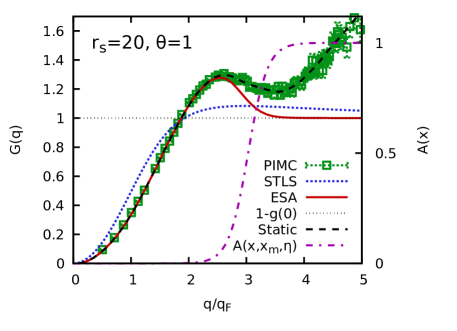
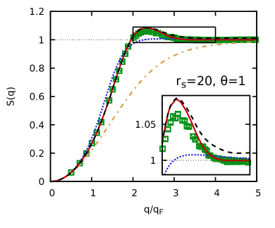
Figure 1: Illustration of the effective static approximation (ESA) Dornheim et al. (2020d) for $r_{s}=20$ and $\theta=1$. Top panel: Static LFC. Green squares are exact PIMC data for $G(q;r_{s},\theta)$ taken from Ref. Dornheim et al. (2020e), and dashed black line the neural net representation from Ref. Dornheim et al. (2019). The solid red curve shows the frequency-averaged LFC $\overline{G}(q;r_{s},\theta)$ within ESA [Eq. (II.4)] and the dotted blue curve the same quantity within STLS Sjostrom and Dufty (2013); Tanaka and Ichimaru (1986). The purple dash-dotted line shows the activation function $A(x,x_{m},\eta)$ [for $x_{m}=\eta=3$, see Eq. (13)] and corresponds to the right $y$-axis. Top panel: Static structure factor $S(q)$ from the same methods, and in RPA (dash-dotted yellow).

An example for the construction of the ESA is shown in Fig. 1 for the UEG at $r_{s}=20$ and $\theta=1$. In the top panel, we show the wave-number dependence of the static LFC $G(q)$, with the green squares depicting exact PIMC data for $N=66$ taken from Ref. Dornheim et al. (2020e) and the black dashed curve the neural-net representation from Ref. Dornheim et al. (2019). Observe the positively increasing tail at large $q$ from both data sets, which is consistent to the positive value of the exchange-correlation contribution to the kinetic energy at these conditions Holas (1987); Militzer and Pollock (2002).

The solid red line corresponds to the ESA and is indistinguishable from the neural net for $q\lesssim 2q_{\textnormal{F}}$. Further, it smoothly goes over into Eq. (11) for larger $q$ and attains this limit for $q\gtrsim 3.5q_{\textnormal{F}}$. The purple dash-dotted curve shows the corresponding activation function $A(x)$ [using $x_{m}=3$] on the right $y$-axis and illustrates the shape of the switchover between the two limits. As a reference, we have also included $\overline{G}(q)$ computed within the finite-temperature version Tanaka and Ichimaru (1986); Sjostrom and Dufty (2013) of the STLS approximation Singwi et al. (1968), see the dotted blue curve. First and foremost, we note that STLS constitutes a purely static theory for the LFC and, thus, exactly fulfills Eq. (11), i.e., it attains a constant value in the limit of large wave numbers, although for significantly larger values of $q$. In addition, STLS is well known to violate the exact compressibility sum-rule Sjostrom and Dufty (2013) (see Eq. (III.2) below) and deviates from the other curves even in the small-$q$ limit. Finally, we note that it does not reproduce the peak of both the neural net and ESA around $q=2.5q_{\textnormal{F}}$.

The bottom panel of Fig. 1 shows the corresponding results for the static structure factor $S(q)$, with the green crosses again being the exact PIMC results from Ref. Dornheim et al. (2020e). At this point, we feel that a note of caution is pertinent. On the one hand, the PIMC method is limited to simulations in the static limit, as dynamic simulations are afflicted with an exponentially hard phase problem Segal et al. (2010) in addition to the usual fermion sign problem Dornheim (2019). Therefore, PIMC results for both $\chi(q,\omega)$ and $G(q,\omega)$ are only available for $\omega=0$. Yet, the PIMC method is also capable to give exact results for frequency-averaged quantities like $S(q)$, as the frequency integration is carried out in the imaginary time Ceperley (1995). Thus, the green squares do correspond to the results one would obtain if the correct, dynamic LFC $G(q,\omega)$ was inserted into Eq. (1).

This is in contrast to the black dashed curve, that has been obtained on the basis of the static approximation, Eq. (10), using as input the neural-net representation Dornheim et al. (2019) of the exact static limit $G(q)$. Evidently, the static treatment of exchange–correlation effects is well justified for $q\lesssim 2q_{\textnormal{F}}$, but there appear systematic deviations for larger $q$; see also the inset showing a magnified segment around the maximum of $S(q)$. In particular, $S(q)$ does not decay to $1$, and, while being small for each individual $q$, the error accumulates under the integral in Eq. (8).

The solid red curve has been obtained by inserting $\overline{G}(q)$ within the ESA into Eq. (10). Plainly, the inclusion of the on-top PDF via Eq. (II.4) removes the spurious effects from the static approximation, and the ESA curve is strikingly accurate over the entire $q$-range.

The dotted blue curve has been computed using $\overline{G}(q)$ within the STLS approximation. For small $q$, it, too obeys the correct parabolic limit Dornheim et al. (2016); Kugler (1970), which is the consequence of perfect screening in the UEG Giuliani and Vignale (2008). For larger $q$, there appear systematic deviations, and the correlation-induced peak of $S(q)$ around $q\sim 2.2q_{\textnormal{F}}$ is not reproduced by this theory; see also Ref. Dornheim et al. (2020e) for an extensive analysis including even stronger values of the coupling strength $r_{s}$.

Finally, the dash-dotted yellow curve has been computed within the RPA. Clearly, neglecting exchange–correlation effects in Eq. (1) leads to an insufficient description of the SSF, and we find systematic deviations of up to $\sim 30\%$.

III Analytical representation of the ESA

III.1 Choice of the activation function

The ESA as it has been defined in Eq. (II.4) has, in principle, two free parameters, which have to be defined/parametrized before an analytical representation of $\overline{G}(q;r_{s},\theta)$ can be introduced. More specifically, these are the transition wave number $x_{m}$ and scaling parameter $\eta$ from the activation function $A(x;x_{m},\eta)$; see Eq. (13).

Scaling parameter $\eta$: We choose $\eta(r_{s},\theta)=3=\textnormal{const}$, as $\overline{G}_{\textnormal{ESA}}(q;r_{s},\theta)$ only weakly depends on this parameter; see Ref. Dornheim et al. (2020d) for an example.

Transition wave-number $x_{m}$: The choice of a reasonable wave-number of the transition between the neural-net and Eq. (11) is less trivial. What we need is a transition around $x_{m}\sim 2.5q_{\textnormal{F}}$ for $\theta\lesssim 1$, whereas it should move to larger wave-number for higher temperatures. The dependence on the density parameter $r_{s}$, on the other hand, is less pronounced and can be neglected. We thus construct the function

$$x_{m}(\theta)=A_{x}+B_{x}\theta+C_{x}\theta^{2}\ ,$$ (14)

with $A_{x}$, $B_{x}$, and $C_{x}$ being free parameters that we determine empirically. In particular, we find $A_{x}=2.64$, $B_{x}=0.31$, and $C_{x}=0.08$. A graphical depiction of Eq. (14) is shown in Fig. 2

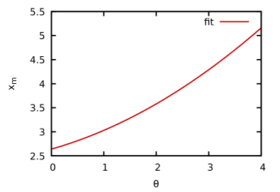
Figure 2: Temperature dependence of the transition wave-number $x_{m}$ from Eq. (14).

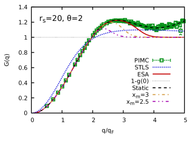
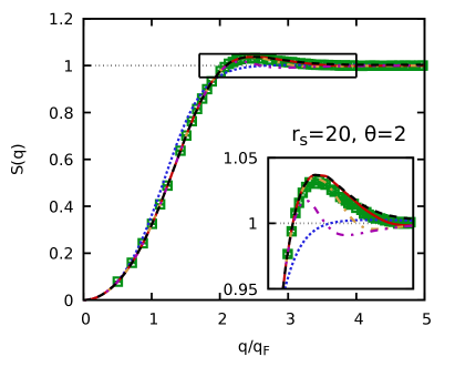
Figure 3: Top panel: Static local field correction for $r_{s}=20$ and $\theta=2$. Green squares are PIMC data for $G(q)$ from Ref. Dornheim et al. (2020e), and dashed black line the neural-net representation from Ref. Dornheim et al. (2019). The solid red line shows $\overline{G}(q)$ within the ESA using Eq. (14) [i.e., $x_{m}=3.58$], and the dash-dotted yellow and dash-double-dotted purple line show the ESA for $x_{m}=3$ and $x_{m}=2.5$. The dotted blue line shows $\overline{G}(q)$ from STLS, and the light grey line the analytical limit from Eq. (11). Bottom panel: Corresponding results for the static structure factor $S(q)$.

An example for the impact of $x_{m}$ on both $\overline{G}(q)$ and the corresponding SSF is shown in Fig. 3. The top panel shows the LFC, and we observe an overall similar trend as for $\theta=1$ depicted in Fig. 1. The main differences both in the PIMC data and the neural net results for $G(q)$ are i) the comparably reduced height of the maximum, ii) the increased width of the maximum regarding $q$, and iii) the decreased slope of the positive tail at large wave numbers. The red curve shows the ESA results for $\overline{G}(q)$ using the transition wave-number obtained from Eq. (14), i.e., $x_{m}\approx 3.58$. In particular, the red curve reproduces the peak structure of the exact static limit $G(q)$, and subsequently approaches the large-$q$ limit from Eq. (11) [light dotted grey line]. In contrast, the dash-dotted yellow and dashed-double-dotted purple lines are ESA results for $x_{m}=3$ and $x_{m}=2.5$, respectively, and start to significantly deviate from $G(q)$ before the peak. Finally, the dotted blue curve shows $\overline{G}(q)$ from STLS, and has been included as a reference.

Regarding $S(q)$, the solid red curve shows the best agreement to the PIMC data, whereas the static approximation again exhibits the spurious behaviour for large $q$, albeit less pronounced than for $\theta=1$ shown above. The ESA results for $x_{m}=3$, too, is in good agreement to the PIMC data, although there appears an unphysical minimum around $q=3q_{\textnormal{F}}$. The ESA curve for $x_{m}=2.5$, on the other hand, does not reproduce the maximum in $S(q)$ from the other data sets. Finally, the STLS curve does not provide an accurate description of the physical behaviour and systematically deviates from the exact results except in the limits of large and small $q$.

III.2 Analytical representation

Let us start this discussion by introducing a suitable functional form for the $q$-dependence of $\overline{G}_{\textnormal{ESA}}$ when $r_{s}$ and $\theta$ are fixed. First and foremost, we note that our parametrization is always constructed from Eq. (II.4), which means that the task at hand is to find an appropriate representation of $G_{\textnormal{nn}}(q;r_{s},\theta)$ that is sufficiently accurate in the wave-number regime where the neural net contributes to the ESA. The correct limit for large $q$, on the other hand, is built in automatically.

In addition, we would like to incorporate the exact long-wavelength limit of the static LFC that is given by the compressibility sum-rule Dornheim et al. (2019); Sjostrom and Dufty (2013) (CSR)

$$\lim_{q\to 0}G(q;r_{s},\theta) = G_{\textnormal{CSR}}(q;r_{s},\theta)$$

$$= -\frac{q^{2}}{4\pi}\frac{\partial^{2}}{\partial n^{2}}\left(nf_{\textnormal{xc}}\right)\quad.$$

This is achieved by the ansatz

$$G^{r_{s},\theta}_{\textnormal{nn,fit}}(q) = G_{\textnormal{CSR}}(q;r_{s},\theta)$$

$$\times\left[\frac{1+\alpha^{r_{s},\theta}x+\beta^{r_{s},\theta}\sqrt{x}}{1+\gamma^{r_{s},\theta}x+\delta^{r_{s},\theta}x^{1.25}+G_{\textnormal{CSR}}(q;r_{s},\theta)}\right]\ ,$$

where $x=q/q_{\textnormal{F}}$ is the reduced wave-number and the super-scripts in the four free parameters $\alpha^{r_{s},\theta}$, $\beta^{r_{s},\theta}$, $\gamma^{r_{s},\theta}$, and $\delta^{r_{s},\theta}$ indicate that they are obtained for fixed values of $\theta$ and $r_{s}$. We note that the $G_{\textnormal{CSR}}(q;r_{s},\theta)$ term in the denominator of the square brackets compensates the equal pre-factor for large $q$.

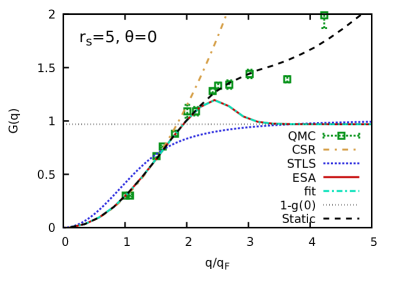
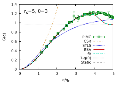
Figure 4: Static local field correction for $r_{s}=5$ and $\theta=0$ (top) and $\theta=3$ (bottom). Green squares are ground-state QMC data from Ref. Moroni et al. (1995) (PIMC data for $G(q)$ from Ref. Dornheim et al. (2019)) for $\theta=0$ ($\theta=3$), and dashed black lines the neural-net representation from Ref. Dornheim et al. (2019). The solid red line shows $\overline{G}(q)$ within the ESA using Eq. (14), and the light blue dash-dotted curve the corresponding fit from Eq. (III.2). The dotted blue line shows $\overline{G}(q)$ from STLS, and the light grey line the analytical limit from Eq. (11).

Two examples for the application of Eq. (III.2) are shown in Fig. 4, where the local field correction is shown for $r_{s}=5$ and $\theta=0$ (top) and $\theta=3$ (bottom). The red curve shows $\overline{G}(q)$ within the ESA, and the light blue dash-dotted curve a fit to these data using Eq. (III.2) as a functional form for $\theta$ and $r_{s}$ being constant. First and foremost, we note that the fit perfectly reproduces the ESA, and no fitting error can be resolved with the naked eye.

The dash-dotted yellow curves show the CSR [Eq. (III.2)], which has been included into Eq. (III.2). In the ground state, we indeed find good agreement between the CSR, the QMC data, the neural net, and also the ESA for $q\lesssim 2q_{\textnormal{F}}$. This is somewhat changed for $\theta=3$, where the yellow curve exhibits more pronounced deviations from the PIMC data and all other curves. Still, we note that the functional form from Eq. (III.2) is capable to accommodate this finding, and attains the small-wave number limit only for small $q$ in this case.

We thus conclude that Eq. (III.2) constitutes a suitable basis for the desired analytical representation $\overline{G}_{\textnormal{ESA}}(q;r_{s},\theta)$. As a next step, we make Eq. (III.2) dependent on the density parameter $r_{s}$. To achieve this goal, we parametrize the free parameters as:

$$\kappa^{\theta}(r_{s})=\frac{a_{\kappa}^{\theta}+b_{\kappa}^{\theta}r_{s}}{1+c_{\kappa}^{\theta}r_{s}}\ ,$$ (17)

with $\kappa\in\{\alpha,\beta,\gamma,\delta\}$. Thus, the characterization of the $r_{s}$-dependence for a single isotherm requires the determination of $12$ free parameters. This results in the isothermic representation of the LFC of the form

$$G^{\theta}_{\textnormal{nn,fit}}( q ;r_{s})=G_{\textnormal{CSR}}(q;r_{s},\theta)$$

$$\times \left[\frac{1+\alpha^{\theta}(r_{s})x+\beta^{\theta}(r_{s})\sqrt{x}}{1+\gamma^{\theta}(r_{s})x+\delta^{\theta}(r_{s})x^{1.25}+G_{\textnormal{CSR}}(q;r_{s},\theta)}\right]\ ,$$

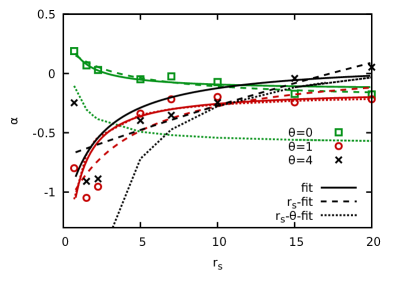
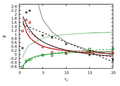
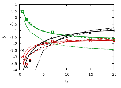
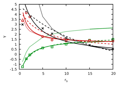
Figure 5: Dependence of the fit parameters $\alpha-\delta$ (clockwise) from Eq. (III.2 on the density parameter $r_{s}$ for $\theta=0$ (green), $\theta=1$ (red), and $\theta=4$ (black). The symbols have been obtained by fitting Eq. (III.2) to ESA data for individual constant values of both $r_{s}$ and $\theta$, and the solid lines have been fitted to these data using Eq. (17) as a functional form. The dashed lines have been obtained from isothermal fits over the full $r_{s}$-range using Eq. (III.2), and the dotted curves from the final fit over the full $r_{s}$-$\theta$-$q$-dependence, see Eq. (III.3).

This isothermic representation is illustrated in Fig. 5, where we show the full $r_{s}$-dependence of the four free parameter $\alpha-\delta$ (clockwise) for $\theta=0$ (green), $\theta=1$ (red), and $\theta=4$ (black). The symbols have been obtained by fitting Eq. (III.2) to ESA data for $\overline{G}(q)$ for constant values of $r_{s}$ and $\theta$. The solid lines have been subsequently obtained by fitting the representation of Eq. (17) to these data over the entire $r_{s}$-range. The resulting curves are indeed smooth and qualitatively capture the main trends from the data points. Finally, the dashed curves have been computed by fitting Eq. (III.2) to ESA data over the entire $r_{s}$-range, but for constant values of $\theta$. Interestingly, this final optimization step results in qualitative change of the description of all four parameters for $\theta=4$, but only mildly changes the results for both $\theta=1$ and $\theta=0$.

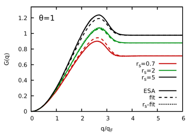
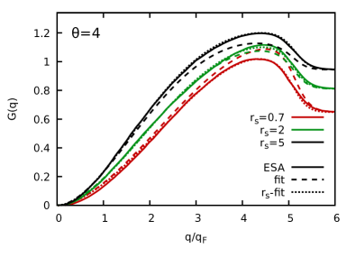
Figure 6: Illustration of the isothermic fit function of the local field correction $\overline{G}_{\textnormal{ESA}}(q)$ for $\theta=1$ (top) and $\theta=4$ (bottom). The red, green, and black curves depict different results for $r_{s}=0.7$, $r_{s}=2$, and $r_{s}=5$, respectively. Solid: ESA; dashed: fitted $r_{s}$-dependence of the individual coefficients $\alpha-\delta$ from Eq. (III.2) according to Eq. (17); dotted: full isothermic fits of $\overline{G}_{\textnormal{ESA}}^{\theta}(q)$ via Eq. (III.2).

Let us for now postpone the discussion of the dotted curve in Fig. 5, and consider Fig. 6 instead. In particular, we show the results of the isothermic fitting procedure for $\theta=1$ (top) and $\theta=4$ (bottom), with the red, green, and black curves corresponding to different data sets for $r_{s}=0.7$, $r_{s}=2$, and $r_{s}=5$, respectively. More specifically, the solid lines show the ESA reference data for $\overline{G}(q)$, and the dashed curves have been obtained by fitting the data points for $\alpha-\delta$ shown in Fig. 5 via Eq. (17). For $\theta=1$, this simple procedure alone leads to an excellent representation of $\overline{G}^{\theta}(q;r_{s})$. The dotted curve has been obtained by performing the full isothermic fits, i.e., by fitting Eq. (III.2) to ESA data over the entire $r_{s}$-range, but with $\theta$ being constant. Indeed, we find only minor deviations between the dashed and the dotted curve.

For $\theta=4$, on the other hand, the simple representation of the fit parameters from Eq. (III.2) results in a substantially less accurate representation of $\overline{G}^{\theta}_{\textnormal{ESA}}(q;r_{s})$, and the systematic error is most pronounced at high density, $r_{s}=0.7$. This shortcoming can be remedied by performing the full isothermic fit of the entire $q$-$r_{s}$-dependence, and the dotted curves are in excellent agreement to the original ESA data everywhere. We thus conclude that the functional form of Eq. (III.2) constitutes an adequate representation of $\overline{G}^{\theta}_{\textnormal{ESA}}(q;r_{s})$.

III.3 Final representation of $\overline{G}_{\textnormal{ESA}}(q;r_{s},\theta)$

The final step is then given by the construction of an analytical representation of the full $r_{s}$-$\theta$-$q$-dependence by expressing the parameters $a_{\kappa}^{\theta}$, $b_{\kappa}^{\theta}$, and $c_{\kappa}^{\theta}$ in Eq. (17) as a function of $\theta$,

$$f_{\kappa}(\theta)=a_{f}+b_{f}\theta+c_{f}\theta^{1.5}\ .$$ (19)

This results in three free parameters for each of the $12$ coefficients required for the characterization of the $r_{s}$-dependence, i.e., a total of $36$ parameters that have to be determined by the fitting procedure.

The full three-dimensional fit-function is then given by

$$G_{\textnormal{nn,fit}}( q ;r_{s},\theta)=G_{\textnormal{CSR}}(q;r_{s},\theta)$$

$$\times \left[\frac{1+\alpha(r_{s},\theta)x+\beta(r_{s},\theta)\sqrt{x}}{1+\gamma(r_{s},\theta)x+\delta(r_{s},\theta)x^{1.25}+G_{\textnormal{CSR}}(q;r_{s},\theta)}\right]\ ,$$

where the functions $\kappa(r_{s},\theta)$ [with $\kappa\in\{\alpha,\beta,\gamma,\delta\}$] are given by

$$\kappa(r_{s},\theta)=\frac{a_{\kappa}(\theta)+b_{\kappa}(\theta)r_{s}}{1+c_{\kappa}(\theta)r_{s}}\ ,$$ (21)

and the $\theta$-dependent coefficients follow Eq. (19).

Table 1: Fit parameters for the analytic parametrization of $\overline{G}_{\textnormal{ESA}}(q;r_{s},\theta)$ from Eq. (III.3). For each of the coefficients $a_{\alpha},b_{\alpha},\dots,c_{\gamma}$, we give the three free parameters from Eq. (19), $a_{f}$, $b_{f}$, and $c_{f}$. A short python implementation is freely available online cod .

	$a_{\alpha}$	$0.66477593$	$-4.59280227$	$1.24649624$
$\alpha$	$b_{\alpha}$	$-1.27089927$	$1.26706839$	$-0.4327608$
	$c_{\alpha}$	$2.09717766$	$1.15424724$	$-0.65356955$
	$a_{\beta}$	$-1.0206202$	$5.16041218$	$-0.23880981$
$\beta$	$b_{\beta}$	$1.07356921$	$-1.67311761$	$0.58928105$
	$c_{\beta}$	$0.8469662$	$1.54029035$	$-0.71145445$
	$a_{\gamma}$	$-2.31252076$	$5.83181391$	$2.29489749$
$\gamma$	$b_{\gamma}$	$1.76614589$	$-0.09710839$	$-0.33180686$
	$c_{\gamma}$	$0.56560236$	$1.10948188$	$-0.43213648$
	$a_{\delta}$	$1.3742155$	$-4.01393906$	$-1.65187145$
$\delta$	$b_{\delta}$	$-1.75381153$	$-1.17022854$	$0.76772906$
	$c_{\delta}$	$0.63867766$	$1.07863273$	$-0.35630091$

Our final analytical representation of the LFC within the effective static approximation immediately follows from plugging Eq. (III.3) into Eq. (II.4),

$$\overline{G}_{\textnormal{ESA,fit}}(q;r_{s},\theta) = G_{\textnormal{nn,fit}}(q;r_{s},\theta)\left(1-A(x)\right)$$

$$+\left(1-g(0;r_{s},\theta)\right)A(x)\ .$$

The thus fitted coefficients are given in Tab. 1, and a corresponding python implementation is freely available online cod .

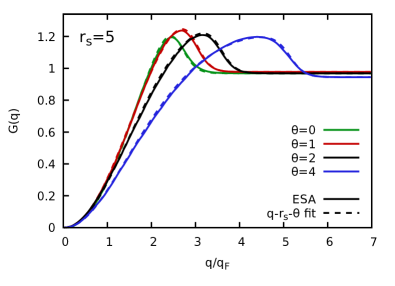
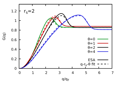
Figure 7: Analytical representation of $\overline{G}_{\textnormal{ESA}}(q;r_{s},\theta)$: Shown are ESA results (solid lines) and our final analytical representation, Eq. (III.3).

The resulting analytical representation $\overline{G}_{\textnormal{ESA}}(q;r_{s},\theta)$ is illustrated in Fig. 7, where we compare it (dashed lines) to the original ESA data at $r_{s}=5$ (top) and $r_{s}=2$, i.e., two metallic densities that are of high interest in the context of WDM research.

More specifically, $r_{s}=5$ corresponds to a strongly coupled system, where an accurate treatment of electronic exchange–correlation effects is paramount Mazevet et al. (2005). These conditions can be realized experimentally in hydrogen jets Zastrau et al. (2014) and evaporation experiments Benage et al. (1999); Karasiev et al. (2016); Mazevet et al. (2005); Desjarlais et al. (2002). The green, red, black, and blue curves show results for $\theta=0$, $\theta=1$, $\theta=2$, and $\theta=4$, respectively, and we find that our new analytical representation of $\overline{G}_{\textnormal{ESA}}(q;r_{s},\theta)$ is in excellent agreement to the ESA input data everywhere.

The bottom panel corresponds to $r_{s}=2$, which is relevant e.g. for the investigation of aluminum Sperling et al. (2015); Ramakrishna et al. (2020b). Here, too, we find excellent agreement between the fitted function and the ESA input data for $\theta=0$ and $\theta=4$, while small, yet significant deviations appear at intermediate wave numbers for $\theta=2$ and $\theta=1$. Still, it is important to note that these deviations do not exceed the statistical uncertainty of the original PIMC input data for $G(q)$ on which the neural net from Ref. Dornheim et al. (2019) and the ESA are based.

We thus conclude that our analytical representation of $\overline{G}_{\textnormal{ESA}}(q;r_{s},\theta)$ provides a highly accurate description of electronic–exchange correlation effects over the entire relevant parameter range. The application of this representation for the computation of other material properties like the static structure factor $S(q)$, interaction energy $v$, or dielectric function $\epsilon(q)$ is discussed in detail in Sec. IV.

IV Results

IV.1 The static local field correction

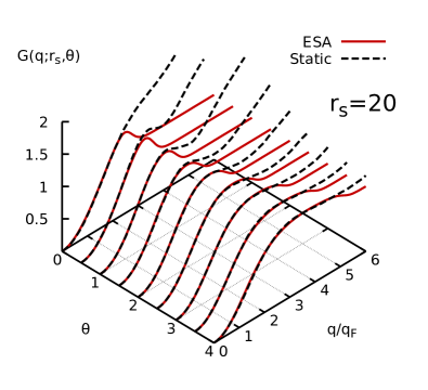
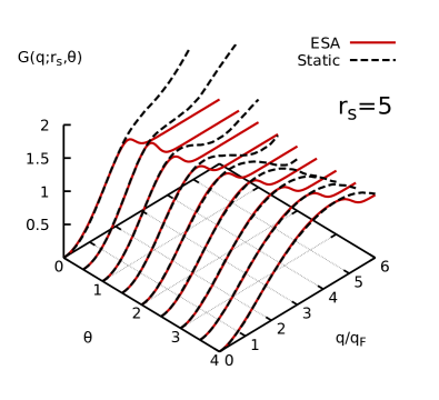
Figure 8: The local field correction in the $\theta$-$q$-plane: The solid red and dashed black curves show our analytical representation of $\overline{G}_{\textnormal{ESA}}(q;r_{s},\theta)$ and the neural-net representation of the exact static limit $G(q)$ from Ref. Dornheim et al. (2019) for $r_{s}=20$ (top) and $r_{s}=5$ (bottom).

Let us begin the investigation of the results that can be obtained within the ESA by briefly recapitulating a few important properties of $\overline{G}_{\textnormal{ESA}}(q;r_{s},\theta)$ itself. To this end, we show the LFC in the $\theta$-$q$-plane for $r_{s}=20$ (top) and $r_{s}=5$ (bottom) in Fig. 8. More specifically, the dashed black lines show the neural-net results for $G(q)$ from Ref. Dornheim et al. (2019), and the solid red lines the corresponding data for our analytical representation of $\overline{G}_{\textnormal{ESA}}(q;r_{s},\theta)$. First and foremost, we note that the temperature dependence is qualitatively similar for both values of the density parameter; a more detailed analysis of the $r_{s}$-dependence of the LFC is presented in Fig. 9 below. As usual, $G(q)$ exhibits a non-constant behaviour for large wave numbers, whereas the ESA converges towards Eq. (11). In addition, our parametrization nicely reproduces the neural-net for $x<x_{m}(\theta)$, which further illustrates the high quality of the representation. Finally, we find that the exact static limit of the LFC, too, becomes increasingly flat at large $q$ for high temperatures, which can be seen particularly well for $r_{s}=20$. In fact, simultaneously considering large values of $r_{s}$ and $\theta$ brings us to the classical limit, where $G(q)$ converges towards one for large wave numbers Ichimaru et al. (1987),

$$\lim_{q\to\infty}G_{\textnormal{classical}}(q)=1\ .$$ (23)

Moreover, the ESA and $G(q)$ converge in this regime as the static structure factor can always be computed from the static LFC only via the exact relation Ichimaru et al. (1987); Mithen et al. (2012)

$$S_{\textnormal{classical}}(q)=\frac{1}{1-\frac{4\pi}{q^{2}}\left[G_{\textnormal{classical}}(q)-1\right]\beta n}\ .$$ (24)

In other words, the spurious effects due to the static approximation and the need for the ESA in WDM applications are a direct consequence of quantum effects on electronic exchange–correlation effects, which only vanish in the classical limit.

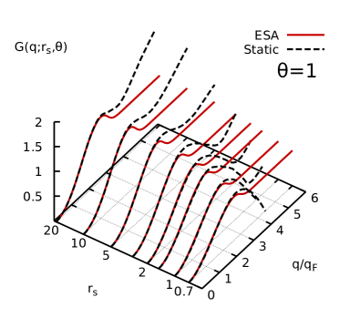
Figure 9: The local field correction in the $r_{s}$-$q$-plane: The solid red and dashed black curves show our analytical representation of $\overline{G}_{\textnormal{ESA}}(q;r_{s},\theta)$ and the neural-net representation of the exact static limit $G(q)$ from Ref. Dornheim et al. (2019) for $\theta=1$. Note the logarithmic scale of the $r_{s}$-axis.

Let us next consider the dependence of the LFC on the density parameter $r_{s}$, which is shown in Fig. 9 for $\theta=1$. For strong coupling, we observe a positive tail in the neural-net results for $G(q)$ which begins at smaller values of $x=q/q_{\textnormal{F}}$ for larger $r_{s}$. Between $r_{s}=2$ and $r_{s}=1$, i.e., in the middle of the WDM regime, this behaviour changes and we find instead a negative slope, which ultimately even leads to negative values of $G(q)$. From a physical perspective, the long wave-number limit is dominated by single-particle effects and the sign of the slope follows from the exchange–correlation contribution to the kinetic energy $K$ Holas (1987); Farid et al. (1993), which changes its sign at these conditions Militzer and Pollock (2002); Hunger et al. (2021).

The ESA, on the other hand, is invariant to this effect and, as usually, attains the consistent limit for $\overline{G}(q)$ given by Eq. (11) for all values of $r_{s}$.

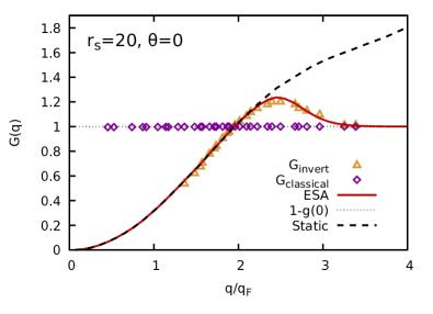
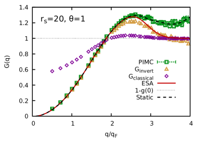
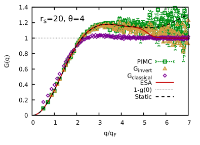
Figure 10: Inverted local field correction at finite temperature: The for $r_{s}=20$ at $\theta=0$ (top), $\theta=1$ (center) and $\theta=4$ (bottom). Green squares and black dashed line: PIMC results for $G(q)$ from Ref. Dornheim et al. (2020e) and corresponding neural-net results Dornheim et al. (2019). Solid red and dotted grey: ESA and large-$q$ limit, Eq. (11). Yellow triangles: inverted LFC $\overline{G}_{\textnormal{classical}}(q)$, see Eq. (25). Purple diamonds: LFC from the classical relation Eq. (26).

As a further motivation for our ESA scheme, we consider an effective local field correction $\overline{G}_{\textnormal{invert}}(q)$, which, by definition, exactly reproduces QMC data for $S(q)$ where they are available. More specifically, such a quantity can be defined as

$$\overline{G}_{\textnormal{invert}}(q)=\textnormal{min}_{\overline{G}}\left(\left|S^{\overline{G}}(q)-S(q)\right|\right)\ ,$$ (25)

where $S^{\overline{G}}(q)$ denotes the SSF computed with respect to some trial static LFC $\overline{G}$. In practice, we solve Eq. (25) by scanning over a dense $\overline{G}$-grid for each $q$-point and search for the minimum deviation in the SSF. In this way, we have effectively inverted $S(q)$ for the LFC $\overline{G}$, even though the relation between the two quantities is not straightforward when quantum mechanical effects cannot be neglected.

The results for this procedure are depicted in Fig. 10, where we show different LFCs at $r_{s}=20$. The top and center panels corresponds to $\theta=0$ and $\theta=1$, and both $G(q)$ and $\overline{G}_{\textnormal{ESA}}(q)$ exhibit the familiar behaviour that has been discussed in the context of Fig. 1 above. The yellow triangles show the inverted results for Eq. (25) and are in remarkably good agreement to both $G(q)$ and $\overline{G}_{\textnormal{ESA}}(q)$ for $q\lesssim 2q_{\textnormal{F}}$. For larger $q$, $\overline{G}_{\textnormal{invert}}(q)$ follows $\overline{G}_{\textnormal{ESA}}(q)$ and attains the same finite limit instead of diverging like the exact static limit of the LFC. In fact, the curves can hardly be distinguished within the given level of accuracy (in particular at $\theta=0$), which further substantiates the simple construction of the ESA, Eq. (II.4).

Let us briefly postpone the discussion of the purple diamonds and instead consider the bottom panel of Fig. 10 showing results for $\theta=4$. At these conditions, $G(q)$ and $\overline{G}_{\textnormal{ESA}}(q)$ only start to noticeably deviate for $q\gtrsim 5q_{\textnormal{F}}$, and the PIMC data, too, appear to remain nearly constant for large $q$. In addition, the black dashed curve is only reliable for $q\leq 5q_{\textnormal{F}}$ as data for larger wave numbers had not been included into the training of the neural net, see Ref. Dornheim et al. (2019) for details.

Unsurprisingly, the inverted data for $\overline{G}_{\textnormal{inverted}}(q)$ closely follow $\overline{G}_{\textnormal{ESA}}(q)$ over the entire $q$-range, and both ESA and the static approximation give highly accurate results for $S(q)$ and $v$.

Let us next more closely examine the connection between the ESA and the classical limit, where $G(q)$ is sufficient to compute exact results for $S(q)$, see Eq. (24) above. In particular, Eq. (24) can be straightforwardly solved for $G(q)$, which gives the relation

$$G_{\textnormal{classical}}(q)=1-\frac{q^{2}}{4\pi}\left(\frac{1}{S(q)}-1\right)\frac{1}{\beta n}\ ,$$ (26)

which, too, is exact in the classical limit.

At the same time, it is interesting to evaluate Eq. (26) for a quantum system to gauge the impact of quantum effects on exchange–correlation effects at different wave numbers $q$. The results are depicted by the purple diamonds in Fig. 10. In the ground state, i.e., $\beta\to\infty$, it holds $G_{\textnormal{classical}}(q)=1$ for all $q$, as the second term is proportional to $T$ and, hence, vanishes. For $\theta=1$, $G_{\textnormal{classical}}(q)$ does depend on $q$, but is still qualitatively wrong over the entire depicted wave-number range. In particular, it strongly violates the compressibility sum-rule Eq. (III.2) and does not even decay to zero in the limit of small $q$. Finally, $G_{\textnormal{classical}}(q)$ does more closely resemble the other curves at $\theta=4$, but still substantially deviates everywhere. We thus conclude that quantum effects are paramount even at $\theta=4$ and $r_{s}=20$, and can only be neglected at significantly higher temperatures.

IV.2 The static structure factor

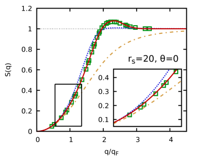
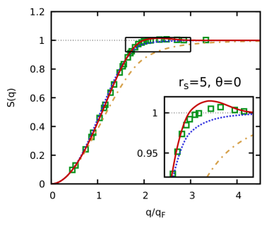
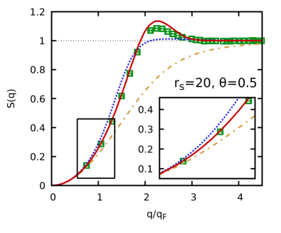
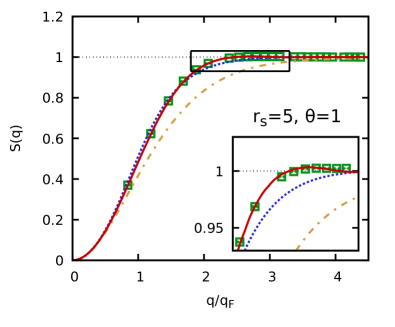
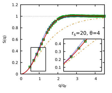
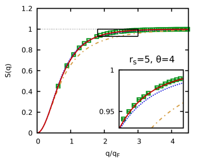
Figure 11: Static structure factor at $r_{s}=20$ (left) and $r_{s}=5$ (right) at different $\theta$. Green squares: $T=0$ QMC data Spink et al. (2013) and finite-$T$ PIMC data Dornheim et al. (2020e); Solid red: ESA; dotted blue: STLS Singwi et al. (1968); Tanaka and Ichimaru (1986); Sjostrom and Dufty (2013); dash-dotted yellow: RPA.

The next quantity to be investigated with the ESA scheme is the static structure factor $S(q)$, which we show in Fig. 11. The left column corresponds to $r_{s}=20$ and, thus, constitutes the most challenging case for the ESA due to the dominant character of exchange–correlation effects at these conditions.

Let us start with the top panel, showing results for the ground state. The green squares are state-of-the-art diffusion Monte Carlo results by Spink et al. Spink et al. (2013) and constitute the gold standard for benchmarks. The solid red curve has been obtained using $\overline{G}_{\textnormal{ESA}}(q)$ and is in remarkable agreement for all $q$, even in the vicinity of the peak of $S(q)$ around $q\approx 2.25q_{\textnormal{F}}$. In contrast, the blue dotted STLS curve does not capture this feature and exhibits pronounced systematic deviations except in the limits of small and large wave numbers.

The center panel in the left column has been obtained for $\theta=0.5$, and the green squares are finite-$T$ PIMC data taken from Dornheim et al. Dornheim et al. (2020e). Again, the ESA gives a very good description of $S(q)$, although the peak height is somewhat overestimated. Still, the description is strikingly improved compared to the STLS approximation.

Lastly, the bottom panel has been obtained for $\theta=4$, where ESA cannot be distinguished from the PIMC reference data within the given Monte Carlo error bars. STLS, too, is quite accurate in this regime, although there remain systematic deviations at intermediate $q$.

Finally, we mention the dash-dotted yellow curve in all three panels, that have been obtained within RPA. Evidently, this mean field description is unsuitable at such low densities even at relatively high values of the reduced temperature $\theta$.

The right column of Fig. 11 has been obtained for a density that is of prime interest to WDM research, $r_{s}=5$. Again, the top panel corresponds to the ground-state and shows relatively good agreement between diffusion Monte Carlo, ESA, and STLS, although the latter does not capture the small correlation induced peak in $S(q)$. The RPA, on the other hand, remains inaccurate despite the reduced coupling strength compared to the left panel.

At $\theta=1$ (center panel), the situation is quite similar, with the ESA being nearly indistinguishable to the PIMC data over the entire $q$-range, whereas STLS is too large for small and too small for large wave numbers.

Finally, the bottom panel corresponds to $\theta=4$. Here, too, only the ESA is capable to reproduce the PIMC data, whereas STLS and in particular RPA exhibit systematic errors.

IV.3 Interaction energy

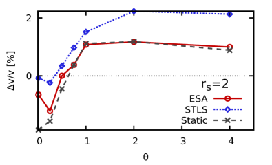
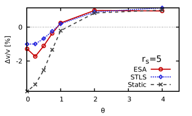
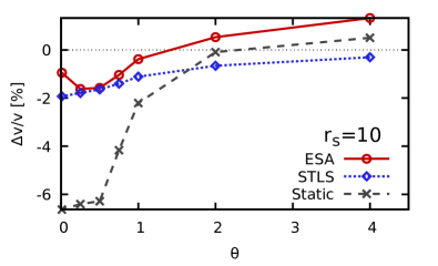
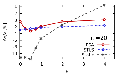
Figure 12: Relative deviation in the interaction energy $v$ [see Eq. (8)] compared to the parametrization by Groth et al. Groth et al. (2017b). Solid red circles: ESA; dotted blue diamonds: STLS Singwi et al. (1968); Tanaka and Ichimaru (1986); Sjostrom and Dufty (2013); dashed grey crosses: static approximation using the neural-net representation from Ref. Dornheim et al. (2019).

The next important quantity to be investigated in this work is the interaction energy $v$, which, in the case of a uniform electron gas, is simply given by a one-dimensional integral over the static structure factor $S(q)$ [see Eq. (8)] that we evaluate numerically. The results are shown in Fig. 12, where we depict the $\theta$-dependence of $v$ for four relevant values of the density parameter $r_{s}$.

More specifically, the top left panel corresponds to $r_{s}=2$, i.e., a metallic density that is typical for WDM experiments using various materials, and we plot the relative deviation in $v$ compared to the accurate parametrization of the UEG by Groth et al. Groth et al. (2017b). At these conditions, both the ESA (solid red) and the static approximation (dashed grey) are very accurate over the entire $\theta$-range, with a maximum deviation of $\Delta v/v\sim 1\%$. The STLS approximation (dotted blue), too, is capable to provide accurate results for $v$, with a maximum deviation of $\sim 2\%$.

Let us proceed to the top right panel corresponding to $r_{s}=5$, a relatively sparse density that can be realized e.g. in experiments with hydrogen jets, see above. First and foremost, we note that both the ESA and STLS provide a remarkably good description of the interaction energy, and the systematic error never exceeds $2\%$. Somewhat surprisingly, STLS even gives slightly more accurate dara for small values of $\theta$ compared to ESA. Yet, this is due to a fortunate cancellation of errors in $S(q)$ under the integral in Eq. (8) [$S(q)$ is too large for small $q$ and too small for large $q$, which roughly balances out] Dornheim et al. (2020d, 2018a), since the static structure factor $S(q)$ is comparatively much better in ESA than in STLS, cf. Fig. 11. In addition, we note that the static approximation performs substantially worse for low temperatures, which is due to the unphysically slow convergence of $S(q)$ towards $1$ for large $q$, see Secs. II.3 and II.4 above.

The bottom left panel shows the same analysis for $r_{s}=10$, and even for this strong coupling strength that constitutes the boundary of the electron liquid regime Dornheim et al. (2018b), the error in ESA does not exceed $2\%$. In addition, the STLS exhibits a comparable accuracy in $v$, whereas the static approximation fails at low $\theta$ as it is expected.

Finally, the bottom right panel shows results for very strong coupling, $r_{s}=20$. Overall, the ESA gives the most accurate data for $v$ of all depicted approximations, and is particularly good both at large temperature and in the ground state. In contrast, the STLS approximation for $\overline{G}(q)$ results in a relatively constant relative deviation of $\sim 2-3\%$, whereas the static approximation cannot reasonably used for this values of the density parameter.

IV.4 Density response function

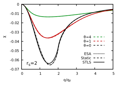
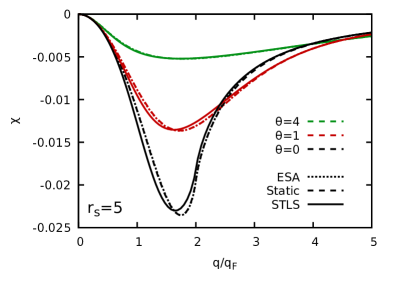
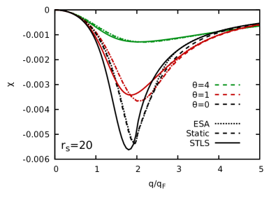
Figure 13: Static density response function $\chi(q)$ for $r_{s}=2$ (top), $r_{s}=5$, and $r_{s}=20$ (bottom). The dotted, solid, and dashed lines have been obtained by inserting into Eq. (10) $\overline{G}_{\textnormal{ESA}}(q)$, $\overline{G}_{\textnormal{STLS}}(q)$, and the neural-net representation of $G(q,0)$ from Ref. Dornheim et al. (2019), respectively. Green curves: $\theta=4$; red: $\theta=1$; black: $\theta=0$.

This section is devoted to a discussion of the suitability of frequency-averaged LFCs for the determination of the exact static limit of the density response function $\chi(q)$. In this case, the previously discussed static approximation, i.e., using the neural-net representation of $G(q,0)$ from Ref. Dornheim et al. (2019), is exact, and the large-$q$ limit of frequency-independent theories $\overline{G}(q)$ given by Eq. (11) is spurious. On the other hand, we might expect that the impact of the LFC decreases for large $q$, such that $\overline{G}_{\textnormal{ESA}}(q)$ and $G(q)$ could potentially give similar results.

To resolve this question, we show $\chi(q)$ in Fig. 13 for three representative values of the density parameter $r_{s}$, with the green, red, and black sets of curves corresponding to $\theta=4$, $\theta=1$, and $\theta=0$, respectively. Let us start with the top panel showing results for a metallic density, $r_{s}=2$, with the dotted, dashed, and solid curves corresponding to ESA, the exact static limit, and STLS, respectively. Firstly, we note that all three curves exhibit the correct parabolic shape for small wave-numbers Kugler (1970),

$$\lim_{q\to 0}\chi(q)=-\frac{4\pi}{q^{2}}\ .$$ (27)

In particular, Eq. (27) is a direct consequence of the $4\pi/q^{2}$ pre-factor in front of the LFC in Eqs. (1) and (10), which means that its impact vanishes for small $q$. With increasing wave numbers, $\chi(q)$ exhibits a broad peak around $q\approx 1.5q_{\textnormal{F}}$, which is also well reproduced by all curves. Moreover, the ESA is virtually indistinguishable from the exact result for all three temperatures, whereas STLS noticeably deviates, in particular at $\theta=0$.

The center panel shows the same analysis for $r_{s}=5$. As discussed above, the increased coupling strength means that the impact of the LFC is more pronounced in this case, and the STLS curve substantially deviates at intermediate wave numbers, except for the highest temperature $\theta=4$. In stark contrast, the ESA is in excellent agreement to the exact curve everywhere, and we find only minor deviations for $2q_{\textnormal{F}}\lesssim q\lesssim 3q_{\textnormal{F}}$. In this sense, the ESA combines the best from two worlds, by giving excellent results both for frequency-averaged quantities like $S(q)$, and really static properties like $\chi(q,0)$ over the entire WDM regime.

This nice feature of the ESA is only lost when entering the strongly coupled electron liquid regime, as it is demonstrated in the bottom panel of Fig. 13 for $r_{s}=20$. In this case, the static density response function is more sharply peaked at low temperature and exhibits a nontrivial shape that is difficult to resolve. Therefore, the STLS approximation is not capable to give a reasonable description of either the peak position or the shape, see Ref. Dornheim et al. (2020e) for a more extensive analysis on this point including even larger values of the density parameter $r_{s}$. The ESA, on the other hand, is strikingly accurate for both $\theta=4$ and $\theta=1$, but substantially deviates from the exact curve for $2q_{\textnormal{F}}\lesssim q\lesssim 4q_{\textnormal{F}}$ in the ground state.

IV.5 Dielectric function

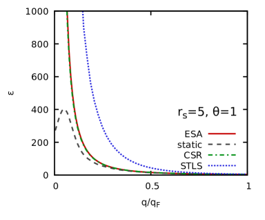
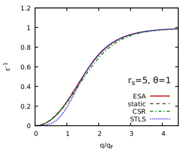
Figure 14: Left: Static dielectric function $\epsilon(q)$ for $r_{s}=5$ and $\theta=1$. Solid red: ESA; dashed grey: exact static limit using the neural-net from Ref. Dornheim et al. (2019); dash-dotted green: CSR, Eq. (III.2); dotted-blue: STLS Sjostrom and Dufty (2013); Tanaka and Ichimaru (1986); Singwi et al. (1968). Right: Same data for the inverse dielectric function $\epsilon^{-1}(q)$.

The dynamic dielectric function $\epsilon(q,\omega)$ is defined as

$$\epsilon(q,\omega)=1-\frac{\chi(q,\omega)}{\frac{q^{2}}{4\pi}+\chi(q,\omega)}\ ,$$ (28)

and is important in both classical and quantum electrodynamics, in particular for the description of plasma oscillations Bonitz (2016); Alexandrov et al. (1984); Hamann et al. (2020b). Since a more detailed analysis of this quantity has been presented elsewhere Hamann et al. (2020a, b), here we restrict ourselves to a brief discussion of ESA results for the static limit of Eq. (28), $\epsilon(q)$.

The results are shown in Fig. 14, where the left panel shows the dielectric function for $r_{s}=5$ and $\theta=1$. Remarkably, we find substantial disagreement between the different results for small wave numbers $q$, which is in striking contrast to linear response properties like $\chi(q)$ and also the SSF $S(q)$. For the latter quantities, the impact of the LFC vanishes for small $q$ as it has been explained above, such that even the mean-field description within the RPA becomes exact in this limit. The dielectric function, on the other hand, always diverges for small $q$, and this divergence is connected to the CSR for the static LFC [Eq. (III.2)] Sjostrom and Dufty (2013); Hamann et al. (2020a),

$$\lim_{q\to 0}\epsilon(q)=-\frac{4\pi\chi_{0}(q)}{q^{2}\left[1+4\pi C\chi_{0}(q)\right]}\ ,$$ (29)

where $C$ is the pre-factor to the parabola in Eq. (III.2),

$$C=-\frac{1}{4\pi}\frac{\partial^{2}}{\partial n^{2}}\left(nf_{\textnormal{xc}}\right)\ .$$ (30)

In principle, exact knowledge of the static LFC as it is encoded in the neural-net representation from Ref. Dornheim et al. (2019) gives access to the exact static dielectric function depicted in Fig. 14. Yet, while the exact relation Eq. (III.2) was indeed incorporated into the training procedure of the neural net, it was not strictly enforced and, thus, is only fulfilled by the static (grey dashed) curve with a finite accuracy. Therefore, this curve violates Eq. (29) and attains a finite value in the limit of $q\to 0$, which is unphysical.

Our new analytical representation of $\overline{G}_{\textnormal{ESA}}(q)$, in contrast, exactly incorporates the CSR, which means that the solid red curve exhibits the correct asymptotic behaviour (depicted as the dash-dotted green curve). Finally, the dotted blue curve has been obtained on the basis of the approximate $\overline{G}_{\textnormal{STLS}}(q)$, and starkly deviates from the exact asymptotic limit. Indeed, the violation of the CSR is a well-known shortcoming of the STLS approach Sjostrom and Dufty (2013), which has ultimately led to the development of the approach by Vashista and Singwi Vashishta and Singwi (1972); Stolzmann and Rösler (2001).

The right panel of Fig. 14 shows the corresponding data for the inverse dielectric function $\epsilon^{-1}(q)$. Here the static and ESA curves are in excellent agreement over the entire $q$-range, which, again, highlights the value of the analytical parametrization which is capable to accurately describe both $\epsilon(q)$ and $\epsilon^{-1}(q)$ at the same time.

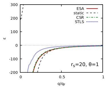
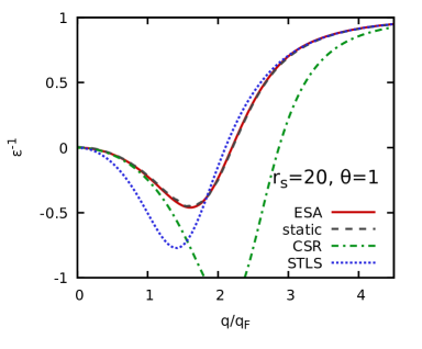
Figure 15: Left: Static dielectric function $\epsilon(q)$ for $r_{s}=20$ and $\theta=1$. Solid red: ESA; dashed grey: exact static limit using the neural-net from Ref. Dornheim et al. (2019); dash-dotted green: CSR, Eq. (III.2); dotted-blue: STLS Sjostrom and Dufty (2013); Tanaka and Ichimaru (1986); Singwi et al. (1968). Right: Same data for the inverse dielectric function $\epsilon^{-1}(q)$.

Let us conclude this section with an example at strong coupling, $r_{s}=20$ and $\theta=1$, depicted in Fig. 15. Firstly, we note that here the ESA and CSR curves for $\epsilon(q)$ diverge towards negative infinity, which is the result of a negative compressibility at these conditions, see also Refs. Hamann et al. (2020a); Sjostrom and Dufty (2013). For completeness, we note that this is a necessary, but not sufficient condition for instability Giuliani and Vignale (2008), and, thus, not problematic. The STLS curve, too, diverges towards negative infinity, although with a substantially different slope. Finally, the static curve becomes increasingly inaccurate for small $q$ and again attains a finite value for $q=0$.

Regarding the inverse dielectric function (right panel), the negative compressibility is reflected by a nontrivial shape of this quantity, with a minimum around $q\approx 1.8q_{\textnormal{F}}$. Here, too, we note that ESA and the static curve are in excellent agreement everywhere, whereas the STLS approximation gives a substantially wrong prediction of both the location and the depth of the minimum in $\epsilon^{-1}(q)$.

IV.6 Dynamic structure factor

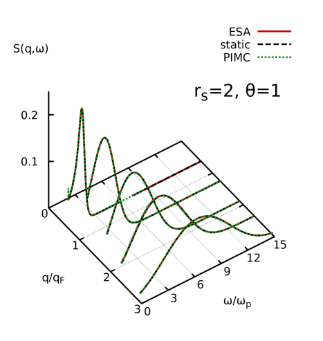
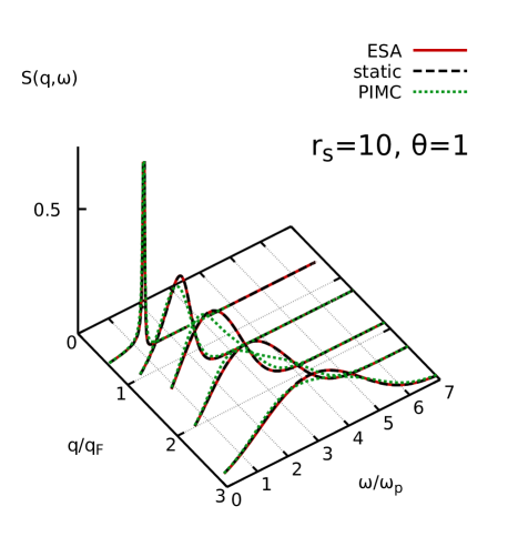
Figure 16: Dynamic structure factor of the uniform electron gas at $\theta=1$ for $r_{s}=2$ (left) and $r_{s}=10$ (right). Solid red: ESA; dashed black: static approximation; dotted green: ab initio reconstructed PIMC results using a stochastically sampled dynamic LFC, taken from Ref. Dornheim et al. (2018b).

The final property of the UEG to be investigated in this work is the dynamic structure factor $S(q,\omega)$, which is shown in Fig. 16 for $\theta=1$. The left panel corresponds to the usual metallic density, $r_{s}=2$, and the dotted green curves are ab initio PIMC results taken from Ref. Dornheim et al. (2018b) that have been obtained by stochastically sampling the dynamic LFC $G(q,\omega)$. In addition, the solid red and dashed black curves have been obtained by using the ESA and the static approximation, and are in virtually perfect agreement to the PIMC data everywhere. This illustrates that a static description of the LFC is fully sufficient to describe the dynamic density response of electrons at these conditions, see also Refs. Dornheim et al. (2018b); Groth et al. (2019); Hamann et al. (2020a); Dornheim and Vorberger (2020) for more details.

The right panel corresponds to a stronger coupling strength, $r_{s}=10$, which is located at the margins of the electron liquid regime. While the ESA and static approximation here, too, basically give the same results, both curves exhibit systematic deviations towards the exact PIMC data. This is a direct consequence of the increased impact of the frequency-dependence of electronic exchange–correlation effects expressed via the dynamic LFC at these conditions Dornheim et al. (2018b).

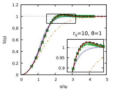
Figure 17: Static structure factor of the UEG for $r_{s}=10$ and $\theta=1$ (cf. right panel of Fig. 16). Green squares: PIMC data taken from Ref. Dornheim et al. (2018b); solid red: ESA; dashed black: static approximation; dotted blue: STLS Singwi et al. (1968); Tanaka and Ichimaru (1986); Sjostrom and Dufty (2013); dash-dotted yellow: RPA.

Interestingly, the impact of the dynamic LFC only manifests in a pronounced way in the shape of $S(q,\omega)$, whereas its normalization [i.e., the SSF, see Eq. (7)] is hardly affected. This is demonstrated in Fig. 17, where we show the corresponding $S(q)$ for the same conditions. For example, for both $q=1.25q_{\textnormal{F}}$ and $q=1.88q_{\textnormal{F}}$, the shape of the PIMC data for $S(q,\omega)$ significantly deviates from the other curves, whereas the SSF is nearly perfectly reproduced by both the ESA and the static approximation.

For larger $q$, the results for the SSF of $G(q)$ and $\overline{G}_{\textnormal{ESA}}(q)$ do start to deviate, but this has no pronounced impact on $S(q,\omega)$ itself.

We thus conclude that both the usual static approximation and our new ESA scheme Dornheim et al. (2020d) are equally well suited for the description of dynamic properties at WDM conditions, but are not suited for a qualitative description of the dynamic density response of the strongly coupled electron liquid regime, for which a fully dynamic local field correction has been shown to be indispensable.

IV.7 Test charge screening.

According to linear response theory, the screened potential of an ion (with charge $Ze$) can be computed using the static dielectric function as Galam and Hansen (1976); Moldabekov et al. (2018a):

$$\Phi(\mathbf{r})=\int\!\frac{\mathrm{d}^{3}q}{(2\pi)^{3}}~{}\frac{4\pi Ze}{q^{2}}\frac{e^{i\mathbf{q}\cdot\mathbf{r}}}{\epsilon(q)},$$ (31)

which is valid for the weak electron-ion coupling. The latter condition is satisfied at large distances from the ion Moldabekov et al. (2020b).

As discussed in Sec. IV.5 above, the violation of the exact limit Eq. (29) leads to the unphysical behavior of the static dielectric function computed using the neural-net representation of the LFC from Ref. Dornheim et al. (2019). This results in incomplete screening when the corresponding static dielectric function is used to compute the screened potential. To illustrate this, we show the screened ion potential (with $Z=1$) for $r_{s}=2$, $\theta=0.5$ and $\theta=1.0$ in Fig. 18, where the screened ion potential is computed using ESA given by Eq. (III.3), the neural-net representation of the LFC from Ref. Dornheim et al. (2019), and RPA.

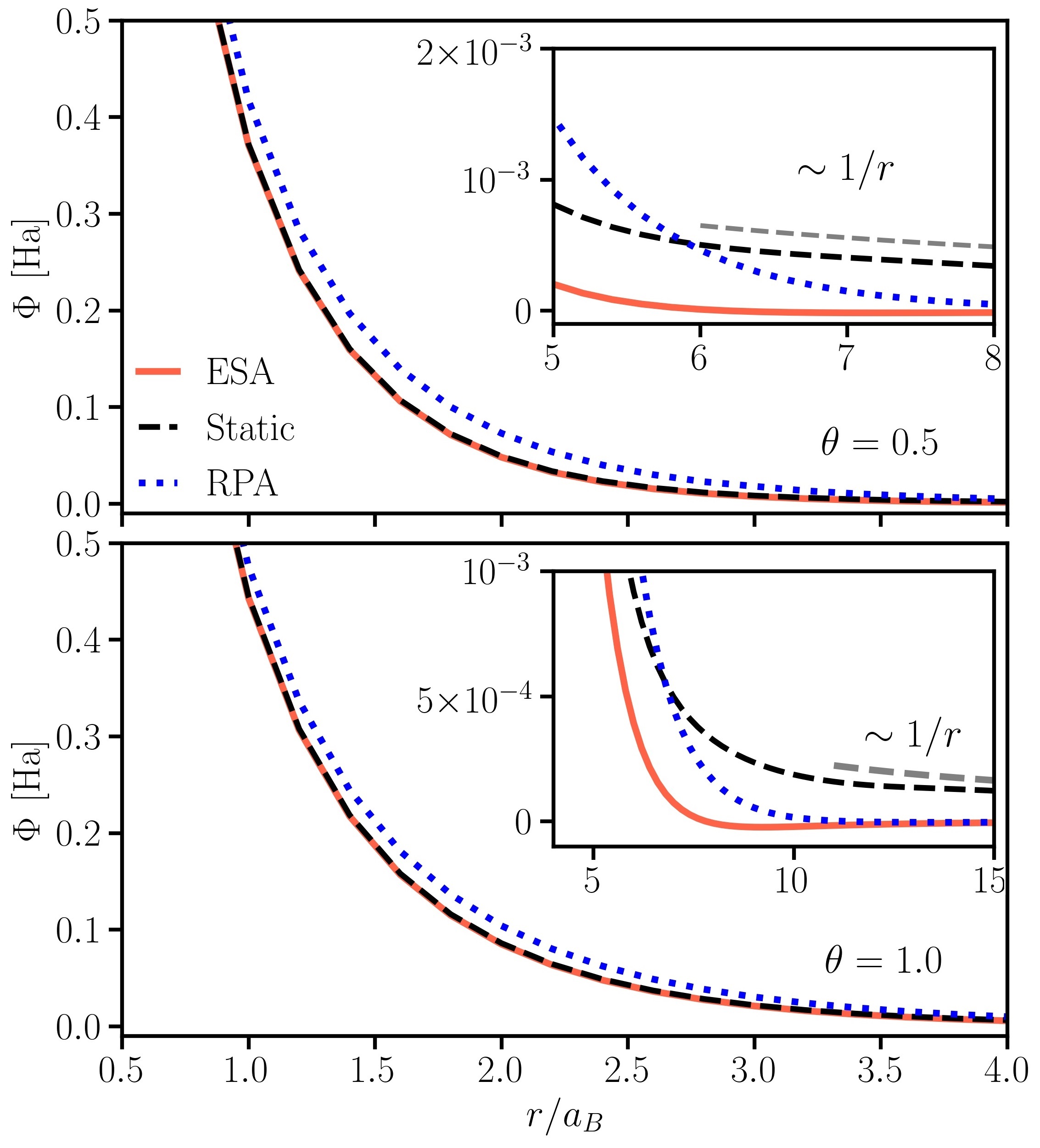
Figure 18: Screened ion potential at $r_{s}=2$, $\theta=0.5$ and $\theta=1$. Solid red: the data computed using the analytical representation of the ESA Eq. (III.3); dashed black: static approximation computed using the neural-net representation of the static local field correction from Ref. Dornheim et al. (2019); dotted blue: RPA result; dashed grey line shows $\sim 1/r$ behavior of the neural-net representation based data at large distances.

From Fig. 18, it is clearly seen that the neural-net representation based result for the screened potential exhibits an $\sim 1/r$ asymptotic behavior at large distances. In contrast, the screened potential obtained using the analytical representation $\overline{G}_{\textnormal{ESA}}(q;r_{s},\theta)$ correctly reproduces complete screening like RPA based data, with a Yukawa type exponential screening at large distances Moldabekov et al. (2020b). Finally, we note that electronic exchange–correlation effects, taken into account by using the LFC, lead to a stronger screening of the ion potential compared to the RPA result Moldabekov et al. (2018a, 2020b, 2017b).

IV.8 Stopping power

A further example for the application of the LFC is the calculation of the stopping power, i.e. the mean energy loss of a projectile (an ion) per unit path length, and related quantities such as the penetration length, straggling rate etc. These energy dissipation characteristics are of paramount importance for such applications as ICF and laboratory astrophysics Grabowski et al. (2020); Kodanova et al. (2018). A linear response expression based on the dynamic dielectric function that describes the stopping power for a low-Z projectile when the ion–electron coupling is weak Arista and Brandt (1981); Zwicknagel et al. (1999) is given by Arista and Brandt (1981):

$$S(v)=\frac{2Z^{2}e^{2}}{\pi v^{2}}\int_{0}^{\infty}\,\frac{{\rm d}k}{k}\,\int_{0}^{kv}{\rm d}\omega~{}\omega~{}{\rm Im}\left[\frac{-1}{\epsilon(k,\omega)}\right],$$ (32)

where $v$ is the ion velocity.

Recently, using Eq. (32), the neural-net representation of the LFC Dornheim et al. (2019) was used to study the ion energy-loss characteristics and friction in a free-electron gas at warm dense matter conditions Moldabekov et al. (2020a). Therefore, it is required to check whether the discussed unphysical behavior of certain quantities based on the neural-net representation of the LFC Dornheim et al. (2019) also manifests in the stopping power. The comparison of the ESA  (III.3) based data for the stopping power to the results obtained using the neural-net representation of the LFC Dornheim et al. (2019) is shown in Fig. 19 for $r_{s}=2$, $\theta=0.5$ and $\theta=1.0$. From Fig. 19 we see that the ESA and the neural-net representation based results for the stopping power are in agreement with a high accuracy. Additionally, a comparison to the RPA based data shows that electronic exchange-correlation effects are significant at projectile velocities $v\lesssim v_{F}$. We refer an interested reader to Ref. Moldabekov et al. (2020a) for a more detailed study in a wider parameter range.

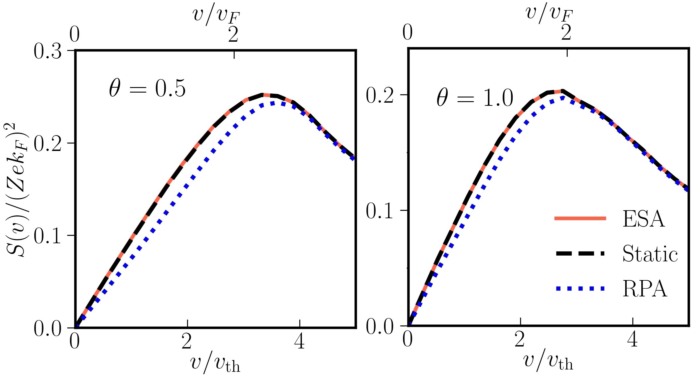
Figure 19: Stopping power at $r_{s}=2$, $\theta=0.5$ and $\theta=1$.Solid red: data computed using the analytical representation of the ESA Eq. (III.3); dashed black: static approximation computed using the neural-net representation of the static local field correction from Ref. Dornheim et al. (2019); dotted blue: RPA result. The lower $x$ axis corresponds to $v/v_{\rm th}$ and the upper $x$ axis to $v/v_{F}$, with $v_{\rm th}$ and $v_{F}$ being the thermal velocity and Fermi velocity of electrons, respectively.

V Summary and Discussion

V.1 Summary

The first main achievement of this work is the construction of an accurate analytical representation of the effective static approximation for the local field correction $\overline{G}_{\textnormal{ESA}}(q;r_{s},\theta)$ covering all wave-numbers and the entire relevant range of densities ($0.7\leq r_{s}\leq 20$) and temperatures ($0\leq\theta\leq 4$). Our fit formula [Eq. (III.3)] well reproduces the original ESA scheme presented in Ref. Dornheim et al. (2020d) while exactly incorporating the CSR in the limit of small wave numbers, and without the need for the evaluation of the neural-net from Ref. Dornheim et al. (2019). A short implementation of Eq. (III.3) in Python is freely available online cod and can easily be incorporated into existing codes; see the next section for a short list of potential applications.

The second aim of this paper is the further analysis of the ESA in general and our fit formula in particular regarding the estimation of various electronic properties. Here one finding of considerable interest has been the estimation of an effective static LFC $\overline{G}_{\textnormal{invert}}(q)$ that, when being inserted into Eq. (1), exactly reproduces the static structure factor $S(q)$ known from QMC calculation both in the ground state and at finite temperature. Remarkably, $\overline{G}_{\textnormal{invert}}(q)$ almost exactly follows $\overline{G}_{\textnormal{ESA}}(q)$ for all wave numbers, which further substantiates the quality of the relatively simple idea behind the ESA. As it is expected, the latter gives very accurate results both for $S(q)$ and the interaction energy $v$, in particular at metallic densities where we find relative deviations to PIMC data not exceeding $1\%$.

A further point of interest is the utility of the ESA regarding the estimation of the static density response function $\chi(q)$ and the directly related dielectric function $\epsilon(q)$. More specifically, the neural-net representation of the exact static LFC $G(q;r_{s},\theta)$ should give exact result for this quantities, whereas the definition of $\overline{G}_{\textnormal{ESA}}(q;r_{s},\theta)$ as a frequency-averaged LFC could potentially introduce a bias in this limit. Yet, we find that the ESA gives virtually exact results over the entire WDM regime (even in the ground-state), whereas said bias only manifests in $\chi(q)$ for the strongly coupled electron liquid regime, $r_{s}=20$. In addition, the exact incorporation of the CSR for small $q$ in our parametrization of $\overline{G}_{\textnormal{ESA}}(q;r_{s},\theta)$ means that the present results for the dielectric function $\epsilon(q)$ are even superior to the corresponding prediction by the neural net, where the CSR is only fulfilled approximately, i.e., with finite accuracy. In particular, the ESA gives the correct divergence behaviour of $\epsilon(q)$ in the limit of small $q$, whereas the neural-net predicts a finite value for $q=0$, which is unphysical Giuliani and Vignale (2008); Hamann et al. (2020a).

A third item of our analysis is the application of the ESA for the estimation of the dynamic structure factor $S(q,\omega)$, where we find no difference to the usual static approximation Dornheim et al. (2018b); Groth et al. (2019); Hamann et al. (2020a). More specifically, both $G(q;r_{s},\theta)$ and $\overline{G}_{\textnormal{ESA}}(q;r_{s},\theta)$ are highly accurate at WDM densities, but cannot reproduce the nontrivial shape of $S(q,\omega)$ associated with the predicted incipient excitonic mode Takada (2016); Higuchi and Yasuhara (2000) in the electron liquid regime.

Furthermore, we have compared our parametrization of $\overline{G}_{\textnormal{ESA}}(q;r_{s},\theta)$ and the neural-net representation of $G(q;r_{s},\theta)$ regarding the construction of an electronically screened ionic potential $\Phi(r)$. While the resulting potentials are in excellent agreement for small to intermediate distances $r$, the aforementioned inaccuracies of the neural net at small $q$ lead to a spuriously slow convergence of $\Phi(r)$ at large ionic separations $r$.

Finally, the stopping power calculation results show that the ESA and the neural-net representation of the LFC are equivalent for this application. Therefore, both the presented analytical fit formula for the ESA and the neural-net representation of the LFC can be used to study ion energy-loss in WDM and hot dense matter.

V.2 Discussion and outlook

The ESA scheme has been shown to give a highly reliable description of electronic XC-effects and, in our opinion, constitutes the method of choice for many applications both in the context of WDM research and solid state physics in the ground state.

Due to its definition as a frequency-averaged LFC, the ESA is particularly suited for the construction of advanced XC-functionals for DFT simulations based on the adiabatic connection and the fluctuation dissipation theorem Lu (2014); Patrick and Thygesen (2015); Pribram-Jones et al. (2016); Görling (2019). This is a highly desirable project, as the predictive capability of DFT for WDM calculations is still limited Ramakrishna et al. (2020b).

Secondly, we mention the interpretation of XRTS experiments Glenzer and Redmer (2009); Kraus et al. (2019) within the Chihara decomposition Chihara (1987) where electronic correlations are often treated insufficiently. In this regard, the remarkable degree of accuracy provided by both ESA and the static approximation, and the promising results for aluminum shown in Ref. Dornheim et al. (2020d) give us hope that an improved description of XRTS signals can be achieved with hardly any additional effort.

Thirdly, the ESA can be used to incorporate electronic XC-effects into many effective theories in a straightforward way. Here examples include quantum hydrodynamics Moldabekov et al. (2018b); Diaw and Murillo (2017); Moldabekov et al. (2015a), average atom models Sterne et al. (2007), electronically screened ionic potentials Moldabekov et al. (2015b, 2016, 2017b), and dynamic electronic phase-field crystal methods Valtierra Rodriguez et al. (2019).

Finally, we mention the value of the LFC in general and the ESA in particular for the estimation of a multitude of material properties like the electronic stopping power Moldabekov et al. (2020a), thermal and electrical conductivities Hamann et al. (2020a), and energy relaxation rates Vorberger et al. (2010); Benedict et al. (2017); Scullard et al. (2018).

From a theoretical perspective, the main open challenge is given by the estimation of the full frequency-dependence of the LFC $G(q,\omega)$, which is currently only possible for certain parameters Dornheim et al. (2018b); Groth et al. (2019); Hamann et al. (2020a). One way towards this goal would be the development of new fermionic QMC approaches at finite temperature, to estimate the imaginary-time density–density correlation function $F(q,\tau)$–the crucial ingredient for the reconstruction of both $S(q,\omega)$ and $G(q,\omega)$. Here the phaseless auxiliary-field QMC method constitutes a promising candidate Lee et al. (2020).

A second topic for future research is given by the comparison of $\overline{G}_{\textnormal{ESA}}(q;r_{s},\theta)$ to different dielectric theories Tanaka (2016); Tanaka and Ichimaru (1986); Sjostrom and Dufty (2013); Tanaka (2017); Stolzmann and Rösler (2001); Panholzer et al. (2018), in particular the recent scheme by Tanaka Tanaka (2016) and the frequency-dependent version of STLS Arora et al. (2017); Schweng and Böhm (1993); Holas and Rahman (1987).

References

- Giuliani and Vignale (2008) G. Giuliani and G. Vignale, Quantum Theory of the Electron Liquid (Cambridge University Press, Cambridge, 2008).
- Foulkes et al. (2001) W. M. C. Foulkes, L. Mitas, R. J. Needs, and G. Rajagopal, “Quantum monte carlo simulations of solids,” Rev. Mod. Phys. 73, 33–83 (2001).
- Loos and Gill (2016) P.-F. Loos and P. M. W. Gill, “The uniform electron gas,” Comput. Mol. Sci 6, 410–429 (2016).
- Dornheim et al. (2018a) T. Dornheim, S. Groth, and M. Bonitz, “The uniform electron gas at warm dense matter conditions,” Phys. Reports 744, 1–86 (2018a).
- Bohm and D. Pines (1952) D. Bohm and A D. Pines, “Collective description of electron interactions: Ii. collective vs individual particle aspects of the interactions,” Phys. Rev. 85, 338 (1952).
- Bardeen et al. (1957) J. Bardeen, L. N. Cooper, and J. R. Schrieffer, “Theory of superconductivity,” Phys. Rev. 108, 1175–1204 (1957).
- Ceperley (1978) D. Ceperley, “Ground state of the fermion one-component plasma: A monte carlo study in two and three dimensions,” Phys. Rev. B 18, 3126–3138 (1978).
- Ceperley and Alder (1980) D. M. Ceperley and B. J. Alder, “Ground state of the electron gas by a stochastic method,” Phys. Rev. Lett. 45, 566–569 (1980).
- Bowen et al. (1994) C. Bowen, G. Sugiyama, and B. J. Alder, “Static dielectric response of the electron gas,” Phys. Rev. B 50, 14838 (1994).
- Moroni et al. (1992) S. Moroni, D. M. Ceperley, and G. Senatore, “Static response from quantum Monte Carlo calculations,” Phys. Rev. Lett 69, 1837 (1992).
- Moroni et al. (1995) S. Moroni, D. M. Ceperley, and G. Senatore, “Static response and local field factor of the electron gas,” Phys. Rev. Lett 75, 689 (1995).
- Ortiz and Ballone (1994) G. Ortiz and P. Ballone, “Correlation energy, structure factor, radial distribution function, and momentum distribution of the spin-polarized uniform electron gas,” Phys. Rev. B 50, 1391–1405 (1994).
- Ortiz et al. (1999) G. Ortiz, M. Harris, and P. Ballone, “Zero temperature phases of the electron gas,” Phys. Rev. Lett. 82, 5317–5320 (1999).
- Zong et al. (2002) F. H. Zong, C. Lin, and D. M. Ceperley, “Spin polarization of the low-density three-dimensional electron gas,” Phys. Rev. E 66, 036703 (2002).
- Shepherd et al. (2012a) James J. Shepherd, George H. Booth, and Ali Alavi, “Investigation of the full configuration interaction quantum monte carlo method using homogeneous electron gas models,” The Journal of Chemical Physics 136, 244101 (2012a), https://doi.org/10.1063/1.4720076 .
- Shepherd et al. (2012b) James J. Shepherd, George Booth, Andreas Grüneis, and Ali Alavi, “Full configuration interaction perspective on the homogeneous electron gas,” Phys. Rev. B 85, 081103 (2012b).
- Spink et al. (2013) G. G. Spink, R. J. Needs, and N. D. Drummond, “Quantum monte carlo study of the three-dimensional spin-polarized homogeneous electron gas,” Phys. Rev. B 88, 085121 (2013).
- Drummond et al. (2004) N. D. Drummond, Z. Radnai, J. R. Trail, M. D. Towler, and R. J. Needs, “Diffusion quantum monte carlo study of three-dimensional wigner crystals,” Phys. Rev. B 69, 085116 (2004).
- Fraser et al. (1996) Louisa M. Fraser, W. M. C. Foulkes, G. Rajagopal, R. J. Needs, S. D. Kenny, and A. J. Williamson, “Finite-size effects and coulomb interactions in quantum monte carlo calculations for homogeneous systems with periodic boundary conditions,” Phys. Rev. B 53, 1814–1832 (1996).
- Perdew and Zunger (1981) J. P. Perdew and Alex Zunger, “Self-interaction correction to density-functional approximations for many-electron systems,” Phys. Rev. B 23, 5048–5079 (1981).
- Perdew and Wang (1992a) John P. Perdew and Yue Wang, “Accurate and simple analytic representation of the electron-gas correlation energy,” Phys. Rev. B 45, 13244–13249 (1992a).
- Perdew and Wang (1992b) John P. Perdew and Yue Wang, “Pair-distribution function and its coupling-constant average for the spin-polarized electron gas,” Phys. Rev. B 46, 12947–12954 (1992b).
- Vosko et al. (1980) S. H. Vosko, L. Wilk, and M. Nusair, “Accurate spin-dependent electron liquid correlation energies for local spin density calculations: a critical analysis,” Canadian Journal of Physics 58, 1200–1211 (1980), https://doi.org/10.1139/p80-159 .
- Gori-Giorgi et al. (2000) Paola Gori-Giorgi, Francesco Sacchetti, and Giovanni B. Bachelet, “Analytic static structure factors and pair-correlation functions for the unpolarized homogeneous electron gas,” Phys. Rev. B 61, 7353–7363 (2000).
- Corradini et al. (1998) M. Corradini, R. Del Sole, G. Onida, and M. Palummo, “Analytical expressions for the local-field factor and the exchange-correlation kernel of the homogeneous electron gas,” Phys. Rev. B 57, 14569 (1998).
- Takada (2016) Yasutami Takada, “Emergence of an excitonic collective mode in the dilute electron gas,” Phys. Rev. B 94, 245106 (2016).
- Perdew et al. (1996) John P. Perdew, Kieron Burke, and Matthias Ernzerhof, “Generalized gradient approximation made simple,” Phys. Rev. Lett. 77, 3865–3868 (1996).
- Burke (2012) Kieron Burke, “Perspective on density functional theory,” The Journal of Chemical Physics 136, 150901 (2012), https://doi.org/10.1063/1.4704546 .
- Jones (2015) R. O. Jones, “Density functional theory: Its origins, rise to prominence, and future,” Rev. Mod. Phys. 87, 897–923 (2015).
- Saumon et al. (1992) D. Saumon, W. B. Hubbard, G. Chabrier, and H. M. van Horn, “The role of the molecular-metallic transition of hydrogen in the evolution of jupiter, saturn, and brown dwarfs,” Astrophys. J 391, 827–831 (1992).
- Militzer et al. (2008) B. Militzer, W. B. Hubbard, J. Vorberger, I. Tamblyn, and S. A. Bonev, “A massive core in jupiter predicted from first-principles simulations,” The Astrophysical Journal 688, L45–L48 (2008).
- Guillot et al. (2018) T. Guillot, Y. Miguel, B. Militzer, W. B. Hubbard, Y. Kaspi, E. Galanti, H. Cao, R. Helled, S. M. Wahl, L. Iess, W. M. Folkner, D. J. Stevenson, J. I. Lunine, D. R. Reese, A. Biekman, M. Parisi, D. Durante, J. E. P. Connerney, S. M. Levin, and S. J. Bolton, “A suppression of differential rotation in jupiter’s deep interior,” Nature 555, 227–230 (2018).
- Becker et al. (2014) A. Becker, W. Lorenzen, J. J. Fortney, N. Nettelmann, M. Schöttler, and R. Redmer, “Ab initio equations of state for hydrogen (h-reos.3) and helium (he-reos.3) and their implications for the interior of brown dwarfs,” Astrophys. J. Suppl. Ser 215, 21 (2014).
- Daligault and Gupta (2009) J. Daligault and S. Gupta, “Electron-ion scattering in dense multi-component plasmas: application to the outer crust of an accreting star,” The Astrophysical Journal 703, 994–1011 (2009).
- Hu et al. (2011) S. X. Hu, B. Militzer, V. N. Goncharov, and S. Skupsky, “First-principles equation-of-state table of deuterium for inertial confinement fusion applications,” Phys. Rev. B 84, 224109 (2011).
- Brongersma et al. (2015) Mark L. Brongersma, Naomi J. Halas, and Peter Nordlander, “Plasmon-induced hot carrier science and technology,” Nature Nanotechnology 10, 25–34 (2015).
- Mukherjee et al. (2013) Shaunak Mukherjee, Florian Libisch, Nicolas Large, Oara Neumann, Lisa V. Brown, Jin Cheng, J. Britt Lassiter, Emily A. Carter, Peter Nordlander, and Naomi J. Halas, “Hot electrons do the impossible: Plasmon-induced dissociation of h2 on au,” Nano Letters 13, 240–247 (2013).
- Falk (2018) K. Falk, “Experimental methods for warm dense matter research,” High Power Laser Sci. Eng 6, e59 (2018).
- Kraus et al. (2016) D. Kraus, A. Ravasio, M. Gauthier, D. O. Gericke, J. Vorberger, S. Frydrych, J. Helfrich, L. B. Fletcher, G. Schaumann, B. Nagler, B. Barbrel, B. Bachmann, E. J. Gamboa, S. Göde, E. Granados, G. Gregori, H. J. Lee, P. Neumayer, W. Schumaker, T. Döppner, R. W. Falcone, S. H. Glenzer, and M. Roth, “Nanosecond formation of diamond and lonsdaleite by shock compression of graphite,” Nature Communications 7, 10970 (2016).
- Kraus et al. (2017) D. Kraus, J. Vorberger, A. Pak, N. J. Hartley, L. B. Fletcher, S. Frydrych, E. Galtier, E. J. Gamboa, D. O. Gericke, S. H. Glenzer, E. Granados, M. J. MacDonald, A. J. MacKinnon, E. E. McBride, I. Nam, P. Neumayer, M. Roth, A. M. Saunders, A. K. Schuster, P. Sun, T. van Driel, T. Döppner, and R. W. Falcone, “Formation of diamonds in laser-compressed hydrocarbons at planetary interior conditions,” Nature Astronomy 1, 606–611 (2017).
- Sperling et al. (2015) P. Sperling, E. J. Gamboa, H. J. Lee, H. K. Chung, E. Galtier, Y. Omarbakiyeva, H. Reinholz, G. Röpke, U. Zastrau, J. Hastings, L. B. Fletcher, and S. H. Glenzer, “Free-electron x-ray laser measurements of collisional-damped plasmons in isochorically heated warm dense matter,” Phys. Rev. Lett. 115, 115001 (2015).
- Graziani et al. (2014) F. Graziani, M. P. Desjarlais, R. Redmer, and S. B. Trickey, eds., Frontiers and Challenges in Warm Dense Matter (Springer, International Publishing, 2014).
- Bonitz et al. (2020) M. Bonitz, T. Dornheim, Zh. A. Moldabekov, S. Zhang, P. Hamann, H. Kählert, A. Filinov, K. Ramakrishna, and J. Vorberger, “Ab initio simulation of warm dense matter,” Physics of Plasmas 27, 042710 (2020), https://doi.org/10.1063/1.5143225 .
- Ott et al. (2018) Torben Ott, Hauke Thomsen, Jan Willem Abraham, Tobias Dornheim, and Michael Bonitz, “Recent progress in the theory and simulation of strongly correlated plasmas: phase transitions, transport, quantum, and magnetic field effects,” The European Physical Journal D 72, 84 (2018).
- Mermin (1965) N. David Mermin, “Thermal properties of the inhomogeneous electron gas,” Phys. Rev. 137, A1441–A1443 (1965).
- Ramakrishna et al. (2020a) Kushal Ramakrishna, Tobias Dornheim, and Jan Vorberger, “Influence of finite temperature exchange-correlation effects in hydrogen,” Phys. Rev. B 101, 195129 (2020a).
- Karasiev et al. (2016) V. V. Karasiev, L. Calderin, and S. B. Trickey, “Importance of finite-temperature exchange correlation for warm dense matter calculations,” Phys. Rev. E 93, 063207 (2016).
- Dharma-wardana (2016) M. W. C. Dharma-wardana, “Current issues in finite-t density-functional theory and warm-correlated matter †,” Computation 4 (2016), 10.3390/computation4020016.
- Sjostrom and Daligault (2014) Travis Sjostrom and Jérôme Daligault, “Gradient corrections to the exchange-correlation free energy,” Phys. Rev. B 90, 155109 (2014).
- Driver and Militzer (2012) K. P. Driver and B. Militzer, “All-electron path integral monte carlo simulations of warm dense matter: Application to water and carbon plasmas,” Phys. Rev. Lett. 108, 115502 (2012).
- Blunt et al. (2014) N. S. Blunt, T. W. Rogers, J. S. Spencer, and W. M. C. Foulkes, “Density-matrix quantum monte carlo method,” Phys. Rev. B 89, 245124 (2014).
- Dornheim et al. (2017a) Tobias Dornheim, Simon Groth, Fionn D. Malone, Tim Schoof, Travis Sjostrom, W. M. C. Foulkes, and Michael Bonitz, “Ab initio quantum monte carlo simulation of the warm dense electron gas,” Physics of Plasmas 24, 056303 (2017a), https://doi.org/10.1063/1.4977920 .
- Brown et al. (2013) Ethan W. Brown, Bryan K. Clark, Jonathan L. DuBois, and David M. Ceperley, “Path-integral monte carlo simulation of the warm dense homogeneous electron gas,” Phys. Rev. Lett. 110, 146405 (2013).
- Dornheim et al. (2015) Tobias Dornheim, Simon Groth, Alexey Filinov, and Michael Bonitz, “Permutation blocking path integral monte carlo: a highly efficient approach to the simulation of strongly degenerate non-ideal fermions,” New Journal of Physics 17, 073017 (2015).
- Schoof et al. (2015) T. Schoof, S. Groth, J. Vorberger, and M. Bonitz, “Ab initio thermodynamic results for the degenerate electron gas at finite temperature,” Phys. Rev. Lett. 115, 130402 (2015).
- Malone et al. (2015) Fionn D. Malone, N. S. Blunt, James J. Shepherd, D. K. K. Lee, J. S. Spencer, and W. M. C. Foulkes, “Interaction picture density matrix quantum monte carlo,” The Journal of Chemical Physics 143, 044116 (2015), https://doi.org/10.1063/1.4927434 .
- Militzer and Driver (2015) Burkhard Militzer and Kevin P. Driver, “Development of path integral monte carlo simulations with localized nodal surfaces for second-row elements,” Phys. Rev. Lett. 115, 176403 (2015).
- Malone et al. (2016) Fionn D. Malone, N. S. Blunt, Ethan W. Brown, D. K. K. Lee, J. S. Spencer, W. M. C. Foulkes, and James J. Shepherd, “Accurate exchange-correlation energies for the warm dense electron gas,” Phys. Rev. Lett. 117, 115701 (2016).
- Dornheim et al. (2016) T. Dornheim, S. Groth, T. Sjostrom, F. D. Malone, W. M. C. Foulkes, and M. Bonitz, “Ab initio quantum Monte Carlo simulation of the warm dense electron gas in the thermodynamic limit,” Phys. Rev. Lett. 117, 156403 (2016).
- Dornheim et al. (2017b) T. Dornheim, S. Groth, and M. Bonitz, “Ab initio results for the static structure factor of the warm dense electron gas,” Contrib. Plasma Phys 57, 468–478 (2017b).
- Groth et al. (2017a) S. Groth, T. Dornheim, and M. Bonitz, “Configuration path integral Monte Carlo approach to the static density response of the warm dense electron gas,” J. Chem. Phys 147, 164108 (2017a).
- Dornheim et al. (2017c) T. Dornheim, S. Groth, J. Vorberger, and M. Bonitz, “Permutation blocking path integral Monte Carlo approach to the static density response of the warm dense electron gas,” Phys. Rev. E 96, 023203 (2017c).
- Driver et al. (2018) K. P. Driver, F. Soubiran, and B. Militzer, “Path integral monte carlo simulations of warm dense aluminum,” Phys. Rev. E 97, 063207 (2018).
- Dornheim et al. (2020a) Tobias Dornheim, Jan Vorberger, and Michael Bonitz, “Nonlinear electronic density response in warm dense matter,” Phys. Rev. Lett. 125, 085001 (2020a).
- Dornheim et al. (2020b) Tobias Dornheim, Michele Invernizzi, Jan Vorberger, and Barak Hirshberg, “Attenuating the fermion sign problem in path integral monte carlo simulations using the bogoliubov inequality and thermodynamic integration,” The Journal of Chemical Physics 153, 234104 (2020b), https://doi.org/10.1063/5.0030760 .
- Lee et al. (2020) Joonho Lee, Miguel A. Morales, and Fionn D. Malone, “A phaseless auxiliary-field quantum monte carlo perspective on the uniform electron gas at finite temperatures: Issues, observations, and benchmark study,” (2020), arXiv:2012.12228 [physics.chem-ph] .
- Liu et al. (2018) Yuan Liu, Minsik Cho, and Brenda Rubenstein, “Ab initio finite temperature auxiliary field quantum monte carlo,” Journal of Chemical Theory and Computation 14, 4722–4732 (2018).
- Yilmaz et al. (2020) A. Yilmaz, K. Hunger, T. Dornheim, S. Groth, and M. Bonitz, “Restricted configuration path integral monte carlo,” The Journal of Chemical Physics 153, 124114 (2020), https://doi.org/10.1063/5.0022800 .
- Groth et al. (2017b) S. Groth, T. Dornheim, T. Sjostrom, F. D. Malone, W. M. C. Foulkes, and M. Bonitz, “Ab initio exchange–correlation free energy of the uniform electron gas at warm dense matter conditions,” Phys. Rev. Lett. 119, 135001 (2017b).
- Karasiev et al. (2014) Valentin V. Karasiev, Travis Sjostrom, James Dufty, and S. B. Trickey, “Accurate homogeneous electron gas exchange-correlation free energy for local spin-density calculations,” Phys. Rev. Lett. 112, 076403 (2014).
- White et al. (2013) T. G. White, S. Richardson, B. J. B. Crowley, L. K. Pattison, J. W. O. Harris, and G. Gregori, “Orbital-free density-functional theory simulations of the dynamic structure factor of warm dense aluminum,” Phys. Rev. Lett. 111, 175002 (2013).
- Gao et al. (2016) Chang Gao, Shen Zhang, Wei Kang, Cong Wang, Ping Zhang, and X. T. He, “Validity boundary of orbital-free molecular dynamics method corresponding to thermal ionization of shell structure,” Phys. Rev. B 94, 205115 (2016).
- Zhang et al. (2016) Shen Zhang, Hongwei Wang, Wei Kang, Ping Zhang, and X. T. He, “Extended application of kohn-sham first-principles molecular dynamics method with plane wave approximation at high energy—from cold materials to hot dense plasmas,” Physics of Plasmas 23, 042707 (2016), https://doi.org/10.1063/1.4947212 .
- Ding et al. (2018) Y. H. Ding, A. J. White, S. X. Hu, O. Certik, and L. A. Collins, “Ab initio studies on the stopping power of warm dense matter with time-dependent orbital-free density functional theory,” Phys. Rev. Lett. 121, 145001 (2018).
- Sharma et al. (2020) Abhiraj Sharma, Sebastien Hamel, Mandy Bethkenhagen, John E. Pask, and Phanish Suryanarayana, “Real-space formulation of the stress tensor for o(n) density functional theory: Application to high temperature calculations,” The Journal of Chemical Physics 153, 034112 (2020), https://doi.org/10.1063/5.0016783 .
- Karasiev et al. (2018) Valentin V. Karasiev, James W. Dufty, and S. B. Trickey, “Nonempirical semilocal free-energy density functional for matter under extreme conditions,” Phys. Rev. Lett. 120, 076401 (2018).
- Glenzer and Redmer (2009) S. H. Glenzer and R. Redmer, “X-ray thomson scattering in high energy density plasmas,” Rev. Mod. Phys 81, 1625 (2009).
- Kraus et al. (2019) D. Kraus, B. Bachmann, B. Barbrel, R. W. Falcone, L. B. Fletcher, S. Frydrych, E. J. Gamboa, M. Gauthier, D. O. Gericke, S. H. Glenzer, S. Göde, E. Granados, N. J. Hartley, J. Helfrich, H. J. Lee, B. Nagler, A. Ravasio, W. Schumaker, J. Vorberger, and T. Döppner, “Characterizing the ionization potential depression in dense carbon plasmas with high-precision spectrally resolved x-ray scattering,” Plasma Phys. Control Fusion 61, 014015 (2019).
- Lu (2014) Deyu Lu, “Evaluation of model exchange-correlation kernels in the adiabatic connection fluctuation-dissipation theorem for inhomogeneous systems,” The Journal of Chemical Physics 140, 18A520 (2014), https://doi.org/10.1063/1.4867538 .
- Patrick and Thygesen (2015) Christopher E. Patrick and Kristian S. Thygesen, “Adiabatic-connection fluctuation-dissipation dft for the structural properties of solids—the renormalized alda and electron gas kernels,” The Journal of Chemical Physics 143, 102802 (2015), https://doi.org/10.1063/1.4919236 .
- Görling (2019) Andreas Görling, “Hierarchies of methods towards the exact kohn-sham correlation energy based on the adiabatic-connection fluctuation-dissipation theorem,” Phys. Rev. B 99, 235120 (2019).
- Pribram-Jones et al. (2016) A. Pribram-Jones, P. E. Grabowski, and K. Burke, “Thermal density functional theory: Time-dependent linear response and approximate functionals from the fluctuation-dissipation theorem,” Phys. Rev. Lett 116, 233001 (2016).
- Gross and Kohn (1985) E. K. U. Gross and W. Kohn, “Local density-functional theory of frequency-dependent linear response,” Phys. Rev. Lett 55, 2850 (1985).
- Baczewski et al. (2016) A. D. Baczewski, L. Shulenburger, M. P. Desjarlais, S. B. Hansen, and R. J. Magyar, “X-ray thomson scattering in warm dense matter without the chihara decomposition,” Phys. Rev. Lett 116, 115004 (2016).
- Moldabekov et al. (2020a) Zh. A. Moldabekov, T. Dornheim, M. Bonitz, and T. S. Ramazanov, “Ion energy-loss characteristics and friction in a free-electron gas at warm dense matter and nonideal dense plasma conditions,” Phys. Rev. E 101, 053203 (2020a).
- Senatore et al. (1996) G. Senatore, S. Moroni, and D.M. Ceperley, “Local field factor and effective potentials in liquid metals,” Journal of Non-Crystalline Solids 205-207, 851 – 854 (1996).
- Moldabekov et al. (2017a) Zh.A. Moldabekov, S. Groth, T. Dornheim, M. Bonitz, and T.S. Ramazanov, “Ion potential in non-ideal dense quantum plasmas,” Contributions to Plasma Physics 57, 532–538 (2017a).
- Moldabekov et al. (2018a) Zh.A. Moldabekov, S. Groth, T. Dornheim, H. Kählert, M. Bonitz, and T. S. Ramazanov, “Structural characteristics of strongly coupled ions in a dense quantum plasma,” Phys. Rev. E 98, 023207 (2018a).
- Hamann et al. (2020a) Paul Hamann, Tobias Dornheim, Jan Vorberger, Zhandos A. Moldabekov, and Michael Bonitz, “Dynamic properties of the warm dense electron gas based on path integral monte carlo simulations,” Phys. Rev. B 102, 125150 (2020a).
- Diaw and Murillo (2017) Abdourahmane Diaw and Michael S. Murillo, “A viscous quantum hydrodynamics model based on dynamic density functional theory,” Scientific Reports 7, 15352 (2017).
- Moldabekov et al. (2018b) Zh. A. Moldabekov, M. Bonitz, and T. S. Ramazanov, “Theoretical foundations of quantum hydrodynamics for plasmas,” Physics of Plasmas 25, 031903 (2018b).
- Sterne et al. (2007) P. A. Sterne, S. B. Hansen, B. G. Wilson, and W. A. Isaacs, “Equation of state, occupation probabilities and conductivities in the average atom purgatorio code,” High Energy Density Physics 3, 278–282 (2007).
- Ceperley (1995) D. M. Ceperley, “Path integrals in the theory of condensed helium,” Rev. Mod. Phys 67, 279 (1995).
- Dornheim et al. (2019) T. Dornheim, J. Vorberger, S. Groth, N. Hoffmann, Zh.A. Moldabekov, and M. Bonitz, “The static local field correction of the warm dense electron gas: An ab initio path integral Monte Carlo study and machine learning representation,” J. Chem. Phys 151, 194104 (2019).
- Groth et al. (2019) S. Groth, T. Dornheim, and J. Vorberger, “Ab initio path integral Monte Carlo approach to the static and dynamic density response of the uniform electron gas,” Phys. Rev. B 99, 235122 (2019).
- Dornheim et al. (2018b) T. Dornheim, S. Groth, J. Vorberger, and M. Bonitz, “Ab initio path integral Monte Carlo results for the dynamic structure factor of correlated electrons: From the electron liquid to warm dense matter,” Phys. Rev. Lett. 121, 255001 (2018b).
- Dornheim and Vorberger (2020) Tobias Dornheim and Jan Vorberger, “Finite-size effects in the reconstruction of dynamic properties from ab initio path integral monte carlo simulations,” Phys. Rev. E 102, 063301 (2020).
- Hamann et al. (2020b) Paul Hamann, Jan Vorberger, Tobias Dornheim, Zhandos A. Moldabekov, and Michael Bonitz, “Ab initio results for the plasmon dispersion and damping of the warm dense electron gas,” Contributions to Plasma Physics 60, e202000147 (2020b).
- Dornheim et al. (2020c) Tobias Dornheim, Zhandos A Moldabekov, Jan Vorberger, and Simon Groth, “Ab initio path integral monte carlo simulation of the uniform electron gas in the high energy density regime,” Plasma Physics and Controlled Fusion 62, 075003 (2020c).
- Dornheim et al. (2020d) Tobias Dornheim, Attila Cangi, Kushal Ramakrishna, Maximilian Böhme, Shigenori Tanaka, and Jan Vorberger, “Effective static approximation: A fast and reliable tool for warm-dense matter theory,” Phys. Rev. Lett. 125, 235001 (2020d).
- Hunger et al. (2021) Kai Hunger, Tim Schoof, Tobias Dornheim, Michael Bonitz, and Alexey Filinov, “Momentum distribution function and short-range correlations of the warm dense electron gas – ab initio quantum monte carlo results,” (2021), arXiv:2101.00842 [physics.plasm-ph] .
- (102) A link to the repository will be given upon publication.
- Kugler (1975) A. A. Kugler, “Theory of the local field correction in an electron gas,” J. Stat. Phys 12, 35 (1975).
- Dornheim et al. (2020e) Tobias Dornheim, Travis Sjostrom, Shigenori Tanaka, and Jan Vorberger, “Strongly coupled electron liquid: Ab initio path integral monte carlo simulations and dielectric theories,” Phys. Rev. B 101, 045129 (2020e).
- Tanaka and Ichimaru (1986) S. Tanaka and S. Ichimaru, “Thermodynamics and correlational properties of finite-temperature electron liquids in the Singwi-Tosi-Land-Sjölander approximation,” J. Phys. Soc. Jpn 55, 2278–2289 (1986).
- Holas (1987) A. Holas, “Exact asymptotic expression for the static dielectric function of a uniform electron liquid at large wave vector,” in Strongly Coupled Plasma Physics, edited by F.J. Rogers and H.E. DeWitt (Plenum, New York, 1987).
- Farid et al. (1993) B. Farid, V. Heine, G. E. Engel, and I. J. Robertson, “Extremal properties of the harris-foulkes functional and an improved screening calculation for the electron gas,” Phys. Rev. B 48, 11602 (1993).
- Sjostrom and Dufty (2013) T. Sjostrom and J. Dufty, “Uniform electron gas at finite temperatures,” Phys. Rev. B 88, 115123 (2013).
- Militzer and Pollock (2002) B. Militzer and E. L. Pollock, “Lowering of the kinetic energy in interacting quantum systems,” Phys. Rev. Lett. 89, 280401 (2002).
- Singwi et al. (1968) K. S. Singwi, M. P. Tosi, R. H. Land, and A. Sjölander, “Electron correlations at metallic densities,” Phys. Rev 176, 589 (1968).
- Segal et al. (2010) Dvira Segal, Andrew J. Millis, and David R. Reichman, “Numerically exact path-integral simulation of nonequilibrium quantum transport and dissipation,” Phys. Rev. B 82, 205323 (2010).
- Dornheim (2019) T. Dornheim, “Fermion sign problem in path integral Monte Carlo simulations: Quantum dots, ultracold atoms, and warm dense matter,” Phys. Rev. E 100, 023307 (2019).
- Kugler (1970) A. A. Kugler, “Bounds for some equilibrium properties of an electron gas,” Phys. Rev. A 1, 1688 (1970).
- Mazevet et al. (2005) S. Mazevet, M. P. Desjarlais, L. A. Collins, J. D. Kress, and N. H. Magee, “Simulations of the optical properties of warm dense aluminum,” Phys. Rev. E 71, 016409 (2005).
- Zastrau et al. (2014) U. Zastrau, P. Sperling, M. Harmand, A. Becker, T. Bornath, R. Bredow, S. Dziarzhytski, T. Fennel, L. B. Fletcher, E. F”orster, S. G”ode, G. Gregori, V. Hilbert, D. Hochhaus, B. Holst, T. Laarmann, H. J. Lee, T. Ma, J. P. Mithen, R. Mitzner, C. D. Murphy, M. Nakatsutsumi, P. Neumayer, A. Przystawik, S. Roling, M. Schulz, B. Siemer, S. Skruszewicz, J. Tiggesb”aumker, S. Toleikis, T. Tschentscher, T. White, M. W”ostmann, H. Zacharias, T. D”oppner, S. H. Glenzer, and R. Redmer, “Resolving ultrafast heating of dense cryogenic hydrogen,” Phys. Rev. Lett 112, 105002 (2014).
- Benage et al. (1999) J. F. Benage, W. R. Shanahan, and M. S. Murillo, “Electrical resistivity measurements of hot dense aluminum,” Phys. Rev. Lett 83, 2953 (1999).
- Desjarlais et al. (2002) M. P. Desjarlais, J. D. Kress, and L. A. Collins, “Electrical conductivity for warm, dense aluminum plasmas and liquids,” Phys. Rev. E 66, 025401(R) (2002).
- Ramakrishna et al. (2020b) Kushal Ramakrishna, Attila Cangi, Tobias Dornheim, and Jan Vorberger, “First-principles modeling of plasmons in aluminum under ambient and extreme conditions,” (2020b), arXiv:2009.12163 [cond-mat.mtrl-sci] .
- Ichimaru et al. (1987) Setsuo Ichimaru, Hiroshi Iyetomi, and Shigenori Tanaka, “Statistical physics of dense plasmas: Thermodynamics, transport coefficients and dynamic correlations,” Physics Reports 149, 91 – 205 (1987).
- Mithen et al. (2012) James P. Mithen, Jérôme Daligault, and Gianluca Gregori, “Comparative merits of the memory function and dynamic local-field correction of the classical one-component plasma,” Phys. Rev. E 85, 056407 (2012).
- Bonitz (2016) M. Bonitz, Quantum kinetic theory (Springer, Heidelberg, 2016).
- Alexandrov et al. (1984) Alexandrov, Bogdankievich, and Rukhadse, Principles of Plasma Electrodynamics (Springer, Heidelberg, Germany, 1984).
- Vashishta and Singwi (1972) P. Vashishta and K. S. Singwi, “Electron correlations at metallic densities v,” Phys. Rev. B 6, 875 (1972).
- Stolzmann and Rösler (2001) W. Stolzmann and M. Rösler, “Static local-field corrected dielectric and thermodynamic functions,” Contrib. Plasma Phys 41, 203 (2001).
- Galam and Hansen (1976) Serge Galam and Jean-Pierre Hansen, “Statistical mechanics of dense ionized matter. vi. electron screening corrections to the thermodynamic properties of the one-component plasma,” Phys. Rev. A 14, 816–832 (1976).
- Moldabekov et al. (2020b) Zh.A. Moldabekov, T. Dornheim, and M. Bonitz, “Screening of a test charge in a free-electron gas at warm dense matter and dense non-ideal plasma conditions,” accepted for publication in Contrib. Plasma Phys.(arXiv:2009.09180) (2020b).
- Moldabekov et al. (2017b) Zh.A. Moldabekov, S. Groth, T. Dornheim, M. Bonitz, and T.S. Ramazanov, “Ion potential in non‐ideal dense quantum plasmas,” Contrib. Plasma Phys. 57, 532–538 (2017b).
- Grabowski et al. (2020) P.E. Grabowski, S.B. Hansen, M.S. Murillo, L.G. Stanton, F.R. Graziani, A.B. Zylstra, S.D. Baalrud, P. Arnault, A.D. Baczewski, L.X. Benedict, C. Blancard, O. Čertík, J. Clérouin, L.A. Collins, S. Copeland, A.A. Correa, J. Dai, J. Daligault, M.P. Desjarlais, M.W.C. Dharma-wardana, G. Faussurier, J. Haack, T. Haxhimali, A. Hayes-Sterbenz, Y. Hou, S.X. Hu, D. Jensen, G. Jungman, G. Kagan, D. Kang, J.D. Kress, Q. Ma, M. Marciante, E. Meyer, R.E. Rudd, D. Saumon, L. Shulenburger, R.L. Singleton, T. Sjostrom, L.J. Stanek, C.E. Starrett, C. Ticknor, S. Valaitis, J. Venzke, and A. White, “Review of the first charged-particle transport coefficient comparison workshop,” High Energy Density Physics 37, 100905 (2020).
- Kodanova et al. (2018) S.K. Kodanova, M.K. Issanova, S.M. Amirov, T.S. Ramazanov, A. Tikhonov, and Zh.A. Moldabekov, “Relaxation of non-isothermal hot dense plasma parameters,” Matter and Radiation at Extremes 3, 40–49 (2018).
- Arista and Brandt (1981) Néstor R. Arista and Werner Brandt, “Energy loss and straggling of charged particles in plasmas of all degeneracies,” Phys. Rev. A 23, 1898–1905 (1981).
- Zwicknagel et al. (1999) G. Zwicknagel, C. Toepffer, and P.-G. Reinhard, “Stopping of heavy ions in plasmas at strong coupling,” Physics Reports 309, 117 – 208 (1999).
- Higuchi and Yasuhara (2000) Masahiko Higuchi and Hiroshi Yasuhara, “Kleinman’s dielectric function and interband optical absorption strength of simple metals,” Journal of the Physical Society of Japan 69, 2099–2106 (2000), https://doi.org/10.1143/JPSJ.69.2099 .
- Chihara (1987) J Chihara, “Difference in x-ray scattering between metallic and non-metallic liquids due to conduction electrons,” Journal of Physics F: Metal Physics 17, 295–304 (1987).
- Moldabekov et al. (2015a) Zhandos Moldabekov, Tim Schoof, Patrick Ludwig, Michael Bonitz, and Tlekkabul Ramazanov, “Statically screened ion potential and bohm potential in a quantum plasma,” Physics of Plasmas 22, 102104 (2015a), https://doi.org/10.1063/1.4932051 .
- Moldabekov et al. (2015b) Zhandos Moldabekov, Patrick Ludwig, Michael Bonitz, and Tlekkabul Ramazanov, “Ion potential in warm dense matter: Wake effects due to streaming degenerate electrons,” Phys. Rev. E 91, 023102 (2015b).
- Moldabekov et al. (2016) Zh. A. Moldabekov, P. Ludwig, M. Bonitz, and T. S. Ramazanov, “Notes on anomalous quantum wake effects,” Contributions to Plasma Physics 56, 442–447 (2016), https://onlinelibrary.wiley.com/doi/pdf/10.1002/ctpp.201500137 .
- Valtierra Rodriguez et al. (2019) Salvador Valtierra Rodriguez, Nan Wang, Nana Ofori-Opoku, Nikolas Provatas, and Kirk H. Bevan, “Capturing the dynamics of wigner crystals within the phase-field crystal method,” Phys. Rev. B 100, 235116 (2019).
- Vorberger et al. (2010) J. Vorberger, D. O. Gericke, Th. Bornath, and M. Schlanges, “Energy relaxation in dense, strongly coupled two-temperature plasmas,” Phys. Rev. E 81, 046404 (2010).
- Benedict et al. (2017) L. X. Benedict, M. P. Surh, L. G. Stanton, C. R. Scullard, A. A. Correa, J. I. Castor, F. R. Graziani, L. A. Collins, O. Certík, J. D. Kress, and M. S. Murillo, “Molecular dynamics studies of electron-ion temperature equilibration in hydrogen plasmas within the coupled-mode regime,” Phys. Rev. E 95, 043202 (2017).
- Scullard et al. (2018) Christian R. Scullard, Susana Serna, Lorin X. Benedict, C. Leland Ellison, and Frank R. Graziani, “Analytic expressions for electron-ion temperature equilibration rates from the Lenard-Balescu equation,” Phys. Rev. E 97, 013205 (2018).
- Tanaka (2016) S. Tanaka, “Correlational and thermodynamic properties of finite-temperature electron liquids in the hypernetted-chain approximation,” J. Chem. Phys 145, 214104 (2016).
- Tanaka (2017) Shigenori Tanaka, “Improved equation of state for finite-temperature spin-polarized electron liquids on the basis of singwi–tosi–land–sjölander approximation,” Contributions to Plasma Physics 57, 126–136 (2017).
- Panholzer et al. (2018) Martin Panholzer, Matteo Gatti, and Lucia Reining, “Nonlocal and nonadiabatic effects in the charge-density response of solids: A time-dependent density-functional approach,” Phys. Rev. Lett. 120, 166402 (2018).
- Arora et al. (2017) P. Arora, K. Kumar, and R. K. Moudgil, “Spin-resolved correlations in the warm-dense homogeneous electron gas,” Eur. Phys. J. B 90, 76 (2017).
- Schweng and Böhm (1993) H. K. Schweng and H. M. Böhm, “Finite-temperature electron correlations in the framework of a dynamic local-field correction,” Phys. Rev. B 48, 2037 (1993).
- Holas and Rahman (1987) A. Holas and S. Rahman, “Dynamic local-field factor of an electron liquid in the quantum versions of the Singwi-Tosi-Land-Sjölander and Vashishta-Singwi theories,” Phys. Rev. B 35, 2720 (1987).