Iterative regularization for constrained minimization formulations of nonlinear inverse problems

Abstract

In this paper we the formulation of inverse problems as constrained minimization problems and their iterative solution by gradient or Newton type. We carry out a convergence analysis in the sense of regularization methods and discuss applicability to the problem of identifying the spatially varying diffusivity in an elliptic PDE from different sets of observations. Among these is a novel hybrid imaging techology known as impedance acoustic tomography, for which we provide numerical experiments.

key words: inverse problems iterative regularization coefficient identification in elliptic PDEs impedance acoustic tomography

1 Introduction

Inverse problems usually consist of a model

$$A(x,u)=0$$ (1)

where the operator $A$ acts on the state $u$ of a system and contains unknown parameters $x$, and an observation equation

$$C(x,u)=y$$ (2)

quantifying the additionally available information that is supposed to allow for identifying the parameters $x$; by a slight notation overload, we will often summarize $(x,u)$ into a single element, which we again call $x$.

The classical formulation of an inverse problem is as an operator equation

$$F(x)=y$$ (3)

where usually $x$ is the searched for parameter (some coefficient, initial or boundary conditions in a PDE or ODE model) but – in an all-at-once formulation – might as well include the state, i.e., the PDE solution. In a conventional reduced setting $F=C\circ S$ is the concatenation of an observation operator $C$ with a parameter-to-state map $S$ satisfying $A(x,S(x))=0$, whereas an all-at-once setting considers the inverse problem as a system $\left\{\begin{array}[]{c}A(x,u)=0\\ C(x,u)=y\end{array}\right.$, which by the above mentioned replacement $x:=(x,u)$ takes the form (3), see, e.g. [10, 11].

We here follow the idea of generalizing this to a formulation of an inverse problem as a constrained minimization problem

$$\min J(x)\mbox{ s.t. }x\in M\,,$$ (4)

where in a reduced type setting, $x$ is the parameter and in an all-at-once-setting $x=(x,u)$ contains both parameter and state. In what follows, it will not be necessary to distinuish between these two cases notationally.

Straightforward instances for equivalent minimization based formulations of (1), (2) are, e.g.,

$$\min\tfrac{1}{2}\|C(x,u)-y\|^{2}\mbox{ s.t. }A(x,u)=0\,,$$

$$\min\tfrac{1}{2}\|A(x,u)\|^{2}\mbox{ s.t. }C(x,u)=y\,,$$ (5)

or in the context of (3) comprising both the reduced $F(x)=C(S(x))$ and the all-at-once $F(x,u)=\left(\begin{array}[]{c}A(x,u)\\ C(x,u)\end{array}\right)$ setting simply

$$\min\tfrac{1}{2}\|F(x)-y\|^{2}\,.$$ (6)

For further examples of such formulations, see., e.g., [12, 21]. In particular we point to the variational formulation according to Kohn and Vogelius, see, e.g, [20].

Here $J$ is a proper functional acting on a Banach space $X$, and we make the normalization assumption

$$J\geq 0\mbox{ on }M\mbox{ and }J(x^{\dagger})=\min_{x\in M}J(x)=0$$ (7)

for $x^{\dagger}$ solving the inverse problem, i.e., we assume to know the minimal value of $J$ (but of course not the minimizer, which is what we intend to retrieve).

The first order optimality condition for a minimizer of (4) is

$$\langle\nabla J(x^{\dagger}),x-x^{\dagger}\rangle\geq 0\quad\mbox{ for all }x\in M\,,$$ (8)

Typically inverse problems also in the form (4) are ill-posed in the sense that solutions to (4) do not depend continuously on the data $y$ that enters the definition of the cost function $J$ and/or of the feasible set $M$. Since in a realistic setting the data is contamianted with measurement noise, i.e., only $y^{\delta}\approx y$ is given, regularization needs to be employed. We first of all do so by possibly adding some regularizing constraints – in particular we think of bound constraints in the sense of Ivanov regularization – and/or by relaxing constraints like fit to the data in the sense of Morozov regularization. In the context of (5), this, e.g., means that we replace $M=\{x\in X\,:\,Cx=y\}$ by $\tilde{M}^{\delta}=\{x\in X\ :\|Cx-y^{\delta}\|\leq\tau\delta\mbox{ and }\tilde{\mathcal{R}}(x)\leq\rho\}$, for the noise level $\delta\geq\|y-y^{\delta}\|$, some constants $\tau>1$, $\rho>0$ and some functional $\tilde{\mathcal{R}}$ satisfying $\tilde{\mathcal{R}}(x^{\dagger})\leq\rho$.

Thus we consider the partly regularized problem

$$\min J^{\delta}(x)\mbox{ s.t. }x\in\tilde{M}^{\delta}$$ (9)

which we intend to solve iteratively, where further regularization is incorporated by early stopping and potentially also by adding regularizing terms during the iteration. As in the above example of $\tilde{M}^{\delta}$, we will generally assume $x^{\dagger}$ to be feasible also for this modified problem, and also approximately minimal

$$x^{\dagger}\in\tilde{M}^{\delta}\mbox{ and }J^{\delta}(x^{\dagger})\leq\eta(\delta)\quad\mbox{ for all }\delta\in(0,\bar{\delta})\,,$$ (10)

$$\mbox{ where }\eta(\delta)>0\mbox{ and }\eta(\delta)\to 0\mbox{ as }\delta\to 0\,.$$

With (9) we formally stay in the same setting as in (4) and, like in (7), assume

$$J^{\delta}\geq 0\mbox{ on }\tilde{M}^{\delta}\,.$$ (11)

The key difference to (4) lies in the fact that $J^{\delta}$ and $\tilde{M}^{\delta}$ might depend on the noise level and this will in fact be crucial since we will study convergence as $\delta$ tends to zero.

Since we consider formulations of inverse problems as constrained minimization problems, an essential step is to consider extensions of iterative methods such as gradient or Newton type methods, to constrained minimization problems. Along with these two paradigms concerning the search direction, we will consider two approaches for guaranteeing feasibility of the sequence, namely projection onto the admissible set in the context of gradient methods in Section 2 and sequential quadratic programming SQP type constrained minimization in Section 3.

Some key reference for gradient, i.e., Landweber type iterative methods are [4] on projected Landweber iteration for linear inverse problems, [6] on (unconstrained) nonlinear Landweber iteration Landweber, and more recently [19] on gradient type methods under very general conditions on the cost function or the forward operator, respectively. Extensions with a penalty term (also allowing for the incorporation of constraints) for linear inverse problems can be found in [3]; For nonlinear problems we also point to [9, 22], however, they do not seem to be applicable to constrained problems, since the penalty term is assumed to be $p$-convex and thus cannot be an indicator function.

Newton type methods for the solution of nonlinear ill-posed problems have been extensively studied in Hilbert spaces (see, e.g., [2, 15] and the references therein) and more recently also in a in Banach space setting. In particular, the iteratively regularized Gauss-Newton method [1] or the Levenberg-Marquardt method [5] easily allow to incorporate constraints in their variational form. Projected Gauss-Newton type methods for constrained ill-posed problems have been considered in, e.g., [14].

The remainder of this paper is organized as follows. In Section 2 we will study a projected version of Landweber iteration, thus a gradient type method in a Hilbert space setting and prove its convergence under certain convexity assumptions on the cost function. Section 3 turns to a general Banach space setting and discusses Newton SQP methods as well as their convergence. Finally, in Section we investigate applicability to the identification of a spatially varying diffusion coefficient in an elliptic PDE from diefferent sets of boundary condtions which leads to three different inverse probems: Inverse groundwater filtration (often also used as a model problem and denoted by $a$-problem) impedance acoustic tomography and electrical impedance tomography. Numerical experiments in Section 5 illustrate our theoretical findings.

2 A projected gradient method

In this section, we consider the projected gradient method for (9)

$$\tilde{x}_{k+1}=x_{k}-\mu_{k}\nabla J^{\delta}(x_{k})\,,\quad x_{k+1}=P_{\tilde{M}^{\delta}}(\tilde{x}_{k+1})$$ (12)

and extend some of the results from [19] to the constrained setting, or from a different viewpoint, extend some of the results from [4] to the nonlinear setting. In (12), $\mu_{k}>0$ is a stepsize parameter and $\nabla J^{\delta}(x_{k})\in X$ is the Riesz representation of ${J^{\delta}}^{\prime}(x_{k})\in X^{*}$ as in this section we restrict ourselves to a Hilbert space setting. The reason for this is the fact that in general Banach spaces, ${J^{\delta}}^{\prime}(x_{k})$ would have to be transported back into $X$ by some duality mapping, which adds nonlinearity and therefore, among others, complicates the choice of the step size, see e.g. [17] for the unconstrained least squares case (6). Moreover, throughout this section we will assume $\tilde{M}^{\delta}$ to be closed and convex and denote by $P_{\tilde{M}^{\delta}}$ the metric (in the Hilbert space setting condsidered in this section also orthogonal) projection onto $\tilde{M}^{\delta}$, which is characterized by the variational inequality

$$x=P_{\tilde{M}^{\delta}}(\tilde{x})\ \Leftrightarrow\ \left(x\in\tilde{M}^{\delta}\mbox{ and }\forall z\in\tilde{M}^{\delta}\,:\ \langle\tilde{x}-x,z-x\rangle\leq 0\right)$$ (13)

With $z:=x_{k}\in\tilde{M}^{\delta}$, this immediately implies

$$0\geq\langle\tilde{x}_{k+1}-x_{k+1},x_{k}-x_{k+1}\rangle=\langle x_{k}-x_{k+1}-\mu_{k}\nabla J^{\delta}(x_{k}),x_{k}-x_{k+1}\rangle$$

hence

$$\|x_{k+1}-x_{k}\|^{2}\leq-\mu_{k}\langle\nabla J^{\delta}(x_{k}),x_{k+1}-x_{k}\rangle$$ (14)

and thus, using the Cauchy-Schwarz inequality, the estimate

$$\|x_{k+1}-x_{k}\|\leq\mu_{k}\|\nabla J^{\delta}(x_{k})\|\,.$$ (15)

Moreover, as well known for (projected) gradient methods, under the Lipschitz type condition on the gradient

$$J^{\delta}(x)-J^{\delta}(x_{+})-\langle\nabla J^{\delta}(x)(x-x_{+})\geq-\tfrac{L}{2}\|x-x_{+}\|^{2}\quad\mbox{ for all }x,x_{+}\in\tilde{M}^{\delta}$$ (16)

for $\mu_{k}\leq\overline{\mu}<\frac{2}{L}$, from (14) we get monotonicity of the cost function values

$$J^{\delta}(x_{k})-J^{\delta}(x_{k+1})\geq(\tfrac{1}{\mu_{k}}-\tfrac{L}{2})\|x_{k+1}-x_{k}\|^{2}$$

and square summability of the steps

$$\sum_{k=0}^{\infty}\|x_{k+1}-x_{k}\|^{2}\leq\frac{1}{\tfrac{1}{\overline{\mu}}-\tfrac{L}{2}}J^{\delta}(x_{0})\,.$$

Monotonicity of the error under additional convexity assumptions easily follows from nonexpansivity of the projection, which yields

$$\|x_{k+1}-x^{\dagger}\|^{2}-\|x_{k}-x^{\dagger}\|^{2}=\|P_{\tilde{M}^{\delta}}(\tilde{x}_{k+1})-P_{\tilde{M}^{\delta}}(x^{\dagger})\|^{2}-\|x_{k}-x^{\dagger}\|^{2}$$ (17)

$$\leq\|\tilde{x}_{k+1}-x^{\dagger}\|^{2}-\|x_{k}-x^{\dagger}\|^{2}=\|\tilde{x}_{k+1}-x_{k}\|^{2}+2\langle\tilde{x}_{k+1}-x_{k},x_{k}-x^{\dagger}\rangle$$

$$=\mu_{k}^{2}\|\nabla J^{\delta}(x_{k})\|^{2}-2\mu_{k}\langle\nabla J^{\delta}(x_{k}),x_{k}-x^{\dagger}\rangle\,.$$

Under the monotonicity condition on $\nabla J^{\delta}$ (i.e., convexity condition on $J^{\delta}$)

$$\langle\nabla J^{\delta}(x)-\nabla J^{\delta}(x^{\dagger}),x-x^{\dagger}\rangle\geq\gamma\|\nabla J^{\delta}(x)\|^{2}\quad\mbox{ for all }x\in\tilde{M}^{\delta}$$ (18)

(which for $\gamma=0$ follows from convexity of $J^{\delta}$, i.e., monotonicity of $\nabla J^{\delta}$) and assuming approximate stationarity

$$\langle\nabla J^{\delta}(x^{\dagger}),x-x^{\dagger}\rangle\geq-\eta(\delta)\quad\mbox{ for all }x\in\tilde{M}^{\delta}\,,$$ (19)

we get from (17), that for all $k\leq k_{*}-1$ with $k_{*}$ defined by

$$k_{*}=k_{*}(\delta)=\min\{k\,:\,\|\nabla J^{\delta}(x_{k})\|^{2}\leq\tau\eta(\delta)\}$$ (20)

the estimate

$$\|x_{k+1}-x^{\dagger}\|^{2}-\|x_{k}-x^{\dagger}\|^{2}$$ (21)

$$\leq\mu_{k}^{2}\|\nabla J^{\delta}(x_{k})\|^{2}-2\mu_{k}\langle\nabla J^{\delta}(x_{k})-\nabla J^{\delta}(x^{\dagger})\rangle+2\mu_{k}\eta(\delta)$$

$$\leq-\mu_{k}(2-\tfrac{\mu_{k}}{\gamma}-\tfrac{2}{\tau\gamma})\langle\nabla J^{\delta}(x_{k})-\nabla J^{\delta}(x^{\dagger}),x_{k}-x^{\dagger}\rangle$$

$$\leq-\mu_{k}(2\gamma-\mu_{k}-\tfrac{2}{\tau})\|\nabla J^{\delta}(x_{k})\|^{2}\leq 0$$

for $\tau>\frac{1}{\gamma}$, $0<\underline{\mu}\leq\mu_{k}\leq\bar{\mu}<2(\gamma-\frac{1}{\tau})$, hence summability

$$\sum_{k=0}^{k_{*}}\langle\nabla J^{\delta}(x_{k})-\nabla J^{\delta}(x^{\dagger}),x_{k}-x^{\dagger}\rangle\leq\frac{1}{\underline{\mu}(2-\frac{\bar{\mu}}{\gamma}-\tfrac{2}{\tau\gamma})}\|x_{0}-x^{\dagger}\|^{2}\,.$$

$$\sum_{k=0}^{k_{*}}\|\nabla J^{\delta}(x_{k})\|^{2}\leq\frac{1}{\underline{\mu}(2\gamma-\bar{\mu}-\tfrac{2}{\tau})}\|x_{0}-x^{\dagger}\|^{2}\,,$$ (22)

Alternatively, under a condition following from (18), (19) and comprising both convexity and approximate stationarity

$$\langle\nabla J^{\delta}(x),x-x^{\dagger}\rangle\geq\gamma\|\nabla J^{\delta}(x)\|^{2}-\eta(\delta)\quad\mbox{ for all }x\in\tilde{M}^{\delta}$$ (23)

which for $k\leq k_{*}-1$ implies

$$(\gamma\tau-1)\eta(\delta)\leq\langle\nabla J^{\delta}(x_{k}),x_{k}-x^{\dagger}\rangle,$$

as well as

$$(1+\tfrac{1}{\gamma\tau-1})\langle\nabla J^{\delta}(x_{k}),x_{k}-x^{\dagger}\rangle\geq\gamma\|\nabla J^{\delta}(x_{k})\|^{2}\,,$$ (24)

we get from (17)

$$\|x_{k+1}-x^{\dagger}\|^{2}-\|x_{k}-x^{\dagger}\|^{2}\leq-\mu_{k}(2-\tfrac{\mu_{k}}{\gamma}(1+\tfrac{1}{\gamma\tau-1}))\langle\nabla J^{\delta}(x_{k}),x_{k}-x^{\dagger}\rangle$$ (25)

$$\leq-\mu_{k}\left(\tfrac{2\gamma}{1+\tfrac{1}{\gamma\tau-1}}-\mu_{k}\right)\|\nabla J^{\delta}(x_{k})\|^{2}\leq 0$$

for $\tau>\frac{1}{\gamma}$, $0<\underline{\mu}\leq\mu_{k}\leq\bar{\mu}<\tfrac{2\gamma}{1+\tfrac{1}{\gamma\tau-1}}$ hence summability

$$\sum_{k=0}^{k_{*}}\langle\nabla J^{\delta}(x_{k}),x_{k}-x^{\dagger}\rangle\leq\frac{1}{\underline{\mu}(2-\tfrac{\bar{\mu}}{\gamma}(1+\tfrac{1}{\gamma\tau-1}))}\|x_{0}-x^{\dagger}\|^{2}\,.$$

which via (24) also implies summability of $\|\nabla J^{\delta}\|^{2}$.

$$\sum_{k=0}^{k_{*}}\|\nabla J^{\delta}\|^{2}\leq(1+\tfrac{1}{\gamma\tau-1})\frac{1}{\gamma\underline{\mu}(2-\tfrac{\bar{\mu}}{\gamma}(1+\tfrac{1}{\gamma\tau-1}))}\|x_{0}-x^{\dagger}\|^{2}\,.$$ (26)

The estimates (22), (26) imply convergence of the gradient to zero as $k\to\infty$ in the noise free case and finiteness of the stopping index $k_{*}$ in case of noisy data. In the noiseless case $\delta=0$ Opial’s Lemma (Lemma 6.1 in the Appendix) with $S=\{x^{*}\in X\,:\,\forall x\in M:\,\langle\nabla J(x^{*}),x-x^{*}\rangle\geq 0\}$, due to monotonicity of $\|x_{k}-x^{*}\|$ and the Bolzano-Weierstrass Theorem, implies weak convergence of $x_{k}$ as $k\to\infty$ to a stationary point. In case of noisy data, one could think of applying the continuous version of Opial’s Lemma (Lemma 6.2 in the Appendix) with $t:=\frac{1}{\delta}$, $x(t):=x_{k_{*}(\delta)}$. However, we do not have monotonicity of the final iterates $x_{k_{*}(\delta)}$ as a function of $\delta$. Still, in case of uniqueness, that is, if $S$ is a singleton $S=\{x^{\dagger}\}$, then boundedness of the sequence $\|x_{k_{*}(\delta)}-x^{*}\|$ by $\|x_{0}-x^{*}\|$ together with a subsequence-subsequence argument yields its weak convergence of $x_{k_{*}(\delta)}$ to $x^{\dagger}$ as $\delta\to 0$.

For this purpose, we have to impose certain continuity assumptions on the cost function and the constrains, namely

$$\mbox{For any sequence }(z_{n})_{n\in\mathbb{N}}\subseteq X\,,\ (\delta_{n})_{n\in\mathbb{N}}\in(0,\bar{\delta}]\,,\ \delta_{n}\to 0\mbox{ as }n\to\infty$$

$$\Bigl{(}\forall n\in\mathbb{N}:\ z_{n}\in\tilde{M}^{\delta_{n}}\mbox{ and }z_{n}\rightharpoonup z\mbox{ and }\nabla J^{\delta_{n}}(z_{n})\to 0\Bigr{)}$$

$$\qquad\qquad\Rightarrow\ \Bigl{(}z\in M\mbox{ and }\forall x\in M:\,\langle\nabla J(z),x-z\rangle\geq 0\Bigr{)}$$ (27)

which in the noiseless case becomes

$$\mbox{For any sequence }(z_{n})_{n\in\mathbb{N}}\subseteq X$$ (28)

$$\Bigl{(}\forall n\in\mathbb{N}:\ z_{n}\in M\mbox{ and }z_{n}\rightharpoonup z\mbox{ and }\nabla J(z_{n})\to 0\Bigr{)}$$

$$\qquad\qquad\Rightarrow\ \Bigl{(}z\in M\mbox{ and }\forall x\in M:\,\langle\nabla J(z),x-z\rangle\geq 0\Bigr{)}$$

Proposition 1

Let (7), (11), (23) hold, and let the sequence of iterates $x_{k}$ be defined by (12) with $k_{*}$ defined by (20).

Then for $\delta=0$ if $M$ and $\nabla J$ satisfy (28), the sequence $(x_{k})_{k\in\mathbb{N}}$ converges weakly to a solution $x^{*}\in M$ of the first order optimality condition (8) as $k\to\infty$.

If $\delta>0$ and additionally (10), (19), and (2) holds, then the family $(x_{k_{*}(\delta)})_{\delta\in(0,\bar{\delta}]}$ converges weakly subsequentially to a stationary point $x^{\dagger}$ according to (8) as $\delta\to 0$. If this stationary point is unique, then the whole sequence converges weakly to $x^{\dagger}$. The same assertion holds with stationarity (8) (with (2)) replaced by

• minimality, i.e., $x^{\dagger}$ (and $z$) $\in\mbox{argmin}\{J(x)\,:\,x\in M\}$

• $\|\nabla J(x^{\dagger})\|=0$ (and $\|\nabla J(z)\|=0$).

Note that case (a) makes uniqueness harder, whereas (b) makes uniqueness easier than (8).

Remark 1

Strong convergence can be shown for the modified projected Landeweber method from [4, Section 3.2]. However, this requires a source condition to hold.

Remark 2

Let us finally comment on the convexity condition (23).

In the special case $J^{\delta}(x)=\tfrac{1}{2}\|F(x)-y^{\delta}\|^{2}$ cf (6), condition (23) becomes

$$\langle F(x)-y^{\delta},F^{\prime}(x)(x-x^{\dagger})\rangle\geq\gamma\|F^{\prime}(x)^{*}(F(x)-y^{\delta})\|^{2}-\eta(\delta)$$ (29)

which, follows, e.g., from

$$\|F^{\prime}(x)\|\leq 1\mbox{ and }$$ (30)

$$\langle F(x)-F(x^{\dagger})-F^{\prime}(x)(x-x^{\dagger}),F(x)-y^{\delta}\rangle\leq(1-\gamma-\kappa)\|F(x)-y^{\delta}\|^{2}$$

with $\|F(x^{\dagger})-y^{\delta}\|\leq 4\kappa\eta(\delta)$. The latter is closely related to the usual normalization and tangential cone conditions for Landweber iteration, see, e.g., [6, 19]. It is, e.g., satisfied for linear $F$ as well as for some specific coefficient identification problems, see, e.g., [6] for the reduced setting, [10] for the all-at-once setting, and [16] for some time dependent problems in both reduced and all-at-once formulation.

3 An SQP type constrained Newton method

A quadratic approximation of the cost function combined with a Tikhonov type additive regularization term yields the iteration scheme

$$x_{k+1}\in X_{k+1}(\alpha):=\mbox{argmin}_{x\in\tilde{M}^{\delta}}Q_{k}^{\delta}(x)+\alpha_{k}\mathcal{R}(x)$$ (31)

$$\mbox{ where }Q_{k}^{\delta}(x)=J^{\delta}(x_{k})+G^{\delta}(x_{k})(x-x_{k})+\tfrac{1}{2}H^{\delta}(x_{k})(x-x_{k})^{2}$$

with

$$G^{\delta}(x_{k}):X\to\mathbb{R}\mbox{ linear },\quad H^{\delta}(x_{k}):X^{2}\to\mathbb{R}\mbox{ bilinear },$$ (32)

$$\mathcal{R}:X\to[0,\infty]\mbox{ proper with domain }\mbox{dom}(\mathcal{R})\supseteq\bigcup_{\delta\in(0,\bar{\delta})}\tilde{M}^{\delta}\cup M$$

where $G^{\delta}$ and $H^{\delta}$ should be viewed as (approximations to) the gradient and Hessian of $J$, $G^{\delta}(x_{k})\approx{J^{\delta}}^{\prime}(x_{k})$, $H^{\delta}(x_{k})\approx{J^{\delta}}^{\prime\prime}(x_{k})$, and $\mathcal{R}$ is a regularization functional. Since we do not necessarily neglect ${J^{\delta}}^{\prime\prime}(x_{k})$, this differs from the iteratively regularized Gauss-Newton method IRGNM studied, e.g., in [1, 18, 13].

Here $X$ is a general Banach space.

To guarantee existence of minimizers, besides (32) we will make the following assumption

Assumption 1

For some topology $\mathcal{T}_{0}$ on $X$

• for all $r\geq\mathcal{R}(x^{\dagger})$, the sublevel set $\tilde{M}^{\delta}_{r}:=\{x\in M^{\delta}\,:\,\mathcal{R}(x)\leq r\}$ is $\mathcal{T}_{0}$ compact.

• the mapping $Q_{k}^{\delta}+\alpha_{k}\mathcal{R}$ is $\mathcal{T}_{0}$ lower semicontinuous

Uniqueness of a minimizer of (31) will not necessarily hold; the sequence $(x_{k})_{k\in\{1,\ldots,k_{*}\}}$ will therefore be defined by an arbitrary selection of minimizers of (31).

The overall iteration is stopped according to the discrepancy principle

$$k_{*}=k_{*}(\delta)=\min\{k\,:\,J^{\delta}(x_{k})\leq\tau\eta(\delta)\}$$ (33)

for some constant $\tau>1$.

As far as the sequence of regularization parameters $\alpha_{k}$ is concerned, we will choose it a priori or a posteriori, see (36), (43) below.

A special case of this with

$$J^{\delta}(x)=\frac{1}{2}\|F(x)-y^{\delta}\|^{2},\quad G^{\delta}(x)h={J^{\delta}}^{\prime}(x)h=\langle F(x)-y^{\delta},F^{\prime}(x)h\rangle,$$ (34)

$${H^{\delta}}(x)(h,\ell)=\langle F^{\prime}(x)h,F^{\prime}(x)\ell\rangle$$

(note that $H^{\delta}$ in general does not coincide with the Hessian of $J^{\delta}$) in Hilbert space is the iteratively regularized Gauss-Newton method for the operator equation formulation (3) of the inverse problem, see, e.g., [1, 18, 13].

Another special case we will consider is the quadratic one

$$J^{\delta}(x)=f^{\delta}+\bar{G}^{\delta}x+\tfrac{1}{2}\bar{H}^{\delta}x^{2},\quad G^{\delta}(x)h=\bar{G}^{\delta}h,\quad{H^{\delta}}(x)(h,\ell)=\bar{H}^{\delta}(h,\ell)$$ (35)

with $f^{\delta}\in X$, $\bar{G}^{\delta}\in L(X,\mathbb{R})=X^{*}$, $\bar{H}^{\delta}\in L(X^{2},\mathbb{R})$, where trivially $Q_{k}^{\delta}$ coincides with $J^{\delta}$.

To provide a convergence analysis, we start with the case of an a priori choice of $\alpha_{k}$

$$\alpha_{k}=\alpha_{0}\theta^{k}$$ (36)

for some $\theta\in(0,1)$ and make, among others, the following assumption.

Assumption 2

For some topology $\mathcal{T}$ on $X$,

• the sublevel set $\{x\in\bigcup_{\delta\in(0,\bar{\delta})}\tilde{M}^{\delta}\,:\,\mathcal{R}(x)\leq R\}=\bigcup_{\delta\in(0,\bar{\delta})}\tilde{M}_{R}^{\delta}$ is $\mathcal{T}$ compact, with $R=(1+\tfrac{a-b}{\tau(a-b)-c}\tfrac{\tau b+c}{(a\theta-b)})\mathcal{R}^{\dagger}+\tfrac{a-b}{\tau(a-b)-c}\tfrac{\tau b+c}{\alpha_{0}}J(x_{0})$ with $\tau$ as in (33), $\alpha_{0}$ as in (36), and $a,b,c$ as in (37);

• $M$ is $\mathcal{T}$ closed with respect to the family of sets $(\tilde{M}^{\delta})_{\delta\in(0,\bar{\delta})}$ in the following sense:

  $$\mbox{For any sequence }(z_{n})_{n\in\mathbb{N}}\subseteq X\,,\ (\delta_{n})_{n\in\mathbb{N}}\in(0,\bar{\delta}]\,,\ \delta_{n}\to 0\mbox{ as }n\to\infty$$

  $$\Bigl{(}\forall n\in\mathbb{N}:\ z_{n}\in\tilde{M}^{\delta_{n}}\mbox{ and }z_{n}\stackrel{{\scriptstyle\mathcal{T}}}{{\longrightarrow}}z\Bigr{)}\Rightarrow z\in M$$

• $\lim_{\delta\to 0}\sup_{x\in M^{\delta}}(J(x)-J^{\delta}(x))\leq 0$;

• $J$ is $\mathcal{T}$ lower semicontinuos.

Comparably to the tangential cone condition in the context of nonlinear Landweber iteration [6] and more recently also the IRGNM [18] we impose a restriction on the nonlinearity / nonconvexity of $J$

$$G^{\delta}(x)(x_{+}-x^{+})+\tfrac{1}{2}H^{\delta}(x)\Bigl{(}(x_{+}-x)^{2}-(x-x^{+})^{2}\Bigr{)}\geq aJ^{\delta}(x_{+})-bJ^{\delta}(x)-cJ^{\delta}(x^{+})$$ (37)

$$\mbox{ for all }x,x_{+}\in\tilde{M}^{\delta},\ x^{+}=x^{\dagger}\,,\quad\delta\in(0,\bar{\delta})\,,$$

with $a>b\geq 0$, $c\geq 0$.

Theorem 3.1

Let conditions (10), (11), (32), (37), and Assumptions 1, 2 hold, assume that $\alpha_{k}$ is chosen a priori according to (36), and $k_{*}$ is chosen according to the discrepancy principle (33), with the following constraints on the constants

$$1>\theta>\frac{b}{a},\quad\tau>\frac{c}{a-b}.$$

Then

• For any $\delta\in(0,\bar{\delta})$, and any $x_{0}\in\bigcap_{\delta\in(0,\bar{\delta})}\tilde{M}^{\delta}\,\cap M$,

  • the iterates $x_{k}$ are well-defined for all $k\leq k_{*}(\delta)$ and $k_{*}(\delta)$ is finite;

  • for all $k\in\{1,\ldots,k_{*}(\delta)\}$ we have

    $$J^{\delta}(x_{k})\leq\tfrac{b}{a}J^{\delta}(x_{k-1})+\tfrac{1}{a}\alpha_{k}\mathcal{R}^{\dagger}+\tfrac{c}{a}\eta;$$

  • for all $k\in\{1,\ldots,k_{*}(\delta)\}$ we have

    $$\mathcal{R}(x_{k})\leq R$$

• As $\delta\to 0$, the final iterates $x_{k_{*}(\delta)}$ tend to a solution of the inverse problem (4) $\mathcal{T}$-subsequentially, i.e., every sequence $x_{k_{*}(\delta_{j})}$ with $\delta_{j}\to 0$ as $j\to\infty$ has a $\mathcal{T}$ convergent subsequence and the limit of every $\mathcal{T}$ convergent subsequence solves (4).

Proof. For any $k\leq k_{*}-1$, existence of a minimizer follows from Assumption 1 by the direct method of calculus of variations. To this end, note that by $x^{\dagger}\in\tilde{M}^{\delta}$, implying

$$\min_{x\in\tilde{M}^{\delta}}Q_{k}(x)+\alpha\mathcal{R}(x)\leq Q_{k}(x^{\dagger})+\alpha\mathcal{R}(x^{\dagger}),$$

and the lower bound

$$Q_{k}(x)\geq Q_{k}(x^{\dagger})+aJ^{\delta}(x)-bJ^{\delta}(x_{k})-cJ^{\delta}(x^{\dagger})\geq Q_{k}(x^{\dagger})-bJ^{\delta}(x_{k})-cJ^{\delta}(x^{\dagger}),$$

which yields

$$\tilde{M}^{\delta}_{r}\supseteq\{x\in\tilde{M}^{\delta}\,:\,Q_{k}(x)+\alpha\mathcal{R}(x)\leq Q_{k}(x^{\dagger})+\alpha\mathcal{R}(x^{\dagger})\}$$

for $r=\mathcal{R}(x^{\dagger})+\frac{1}{\alpha}(bJ^{\delta}(x_{k})+cJ^{\delta}(x^{\dagger}))$, it suffices to restrict the search for a minimizer to the set $\tilde{M}^{\delta}_{r}$ as defined in Assumption 1.

For a hence existing minimizer $x_{k+1}$, its minimality together with feasibility of $x^{\dagger}$ for (31) yields

$$G^{\delta}(x_{k})(x_{k+1}-x_{k})+\tfrac{1}{2}H^{\delta}(x_{k})(x_{k+1}-x_{k})^{2}+\alpha_{k}\mathcal{R}(x_{k+1})$$ (38)

$$\leq G^{\delta}(x_{k})(x^{\dagger}-x_{k})+\tfrac{1}{2}H^{\delta}(x_{k})(x^{\dagger}-x_{k})^{2}+\alpha_{k}\mathcal{R}(x^{\dagger}),$$

which with (37) implies

$$aJ^{\delta}(x_{k+1})+\alpha_{k}\mathcal{R}(x_{k+1})\leq bJ^{\delta}(x_{k})+cJ^{\delta}(x^{\dagger})+\alpha_{k}\mathcal{R}(x^{\dagger})$$ (39)

thus, with the a priori choice (36), and (10), abbreviating $J_{k}=J^{\delta}(x_{k})$, $\mathcal{R}_{k}=\mathcal{R}(x_{k})$, $\mathcal{R}^{\dagger}=\mathcal{R}(x^{\dagger})$

$$J_{k+1}+\tfrac{\alpha_{0}}{a}\theta^{k}\mathcal{R}_{k+1}\leq\tfrac{b}{a}J_{k}+\tfrac{\alpha_{0}}{a}\theta^{k}\mathcal{R}^{\dagger}+\tfrac{c}{a}\eta\,.$$ (40)

Inductively, with $\mathcal{R}\geq 0$, we conclude that for all $k\leq k_{*}$

$$J_{k} \leq(\tfrac{b}{a})^{k}J_{0}+\tfrac{\alpha_{0}}{a}\mathcal{R}^{\dagger}\sum_{j=0}^{k-1}(\tfrac{b}{a})^{j}\theta^{k-1-j}+\tfrac{c}{a}\eta\sum_{j=0}^{k-1}(\tfrac{b}{a})^{j}$$ (41)

$$\leq(\tfrac{b}{a})^{k}J_{0}+\tfrac{\alpha_{0}}{a\theta-b}\mathcal{R}^{\dagger}\theta^{k}+\tfrac{c}{a-b}\eta\,.$$

Using the minimality of $k_{*}$ according to (33), we get, for all $k\leq k_{*}-1$, that $\eta\leq\frac{J_{k}}{\tau}$ and therefore, together with (41)

$$(1-\tfrac{c}{\tau(a-b)})J_{k}\leq(\tfrac{b}{a})^{k}J_{0}+\tfrac{\alpha_{0}}{a\theta-b}\mathcal{R}^{\dagger}\theta^{k}\,.$$

Inserting this back into (40) with $J^{\delta}\geq 0$, after multiplication by $\frac{a}{\alpha_{k}}$ and again using (33) yields

$$\mathcal{R}_{k+1} \leq\tfrac{b}{\alpha_{k}}J_{k}+\mathcal{R}^{\dagger}+\tfrac{c}{\alpha_{k}}\tfrac{J_{k}}{\tau}\leq\mathcal{R}^{\dagger}+\tfrac{\tau b+c}{\tau\alpha_{0}}\theta^{-k}J_{k}$$ (42)

$$\leq\mathcal{R}^{\dagger}+\tfrac{a-b}{\tau(a-b)-c}\tfrac{\tau b+c}{\alpha_{0}}\Bigl{(}(\tfrac{b}{a\theta})^{k}J_{0}+\tfrac{\alpha_{0}}{a\theta-b}\mathcal{R}^{\dagger}\Bigr{)}=R$$

for all $k\leq k_{*}-1$.

From (41), which holds for all $k\leq k_{*}$ and $\tau>\tfrac{c}{a-b}$, as well as $\tfrac{b}{a}<\theta$, we conclude that the stopping index according to (33) is reached after finitely many, namely at most $\frac{\log((\tau-\tfrac{c}{a-b})\eta)-\log(J_{0}+\tfrac{\alpha_{0}}{a\theta-b}\mathcal{R}^{\dagger})}{\log\theta}$ steps.

Setting $k=k_{*}-1$ in (42) yields $\mathcal{R}(x_{k_{*}(\delta)})\leq R$, which implies $\mathcal{T}$ convergence of a subsequence $x^{j}$ of $x_{k_{*}(\delta)}$ to some $\bar{x}$, which by Assumption 2 lies in $M$.

By definition of $k_{*}$ and (10) we have $J(x_{k_{*}(\delta)})\leq\tau\eta(\delta)+J(x_{k_{*}(\delta)})-J^{\delta}(x_{k_{*}(\delta)})\to 0$ as $\delta\to 0$; $\mathcal{T}$ lower semicontinuity therefore yields $J(\bar{x})=0$.

$\diamondsuit$

We now consider convergence with an a posteriori according choice of $\alpha_{k}$ according to the discrepancy principle type rule (which can also be interpreted as an inexact Newton condition)

$$\underline{\sigma}\leq\sigma_{k}(\alpha_{k}):=\frac{Q_{k}^{\delta}(X_{k+1}(\alpha_{k}))}{J^{\delta}(x_{k})}\leq\overline{\sigma}$$ (43)

with $0<\underline{\sigma}<\overline{\sigma}<1$; note that in (43), the denominator of $\sigma_{k}(\alpha_{k})$ will be positive and bounded away from zero by $\tau\eta(\delta)$ for all $k\leq k_{*}(\delta)-1$ by (33). In order to obtain well-definedness of $\sigma_{k}(\alpha)$ as a function of $\alpha$, we will assume that the mapping

$$\alpha\mapsto Q_{k}^{\delta}(X_{k+1}(\alpha))\mbox{ with }X_{k+1}(\alpha)=\mbox{argmin}_{x\in\tilde{M}^{\delta}}(Q_{k}^{\delta}(x)+\alpha\mathcal{R}(x))$$

is single valued, which is, e.g., the case if the minimizer of $Q_{k}^{\delta}(x)+\alpha\mathcal{R}(x)$ over $\tilde{M}^{\delta}$ is unique. The latter can be achieved, e.g., by assuming convexity of $Q_{k}^{\delta}$ – choosing $H^{\delta}$ as a positive semidefinite approximation of the (not necessarily positive semidefinite) true Hessian ${J^{\delta}}^{\prime\prime}$ – and strict convexity of $\mathcal{R}$.

For the a posteriori choice (43) we have to slightly modify the setting to guarantee existence of $\alpha_{k}$ such that (43) holds. The latter is possible if for some appropriate point $x^{*}$, the quotient $\frac{Q^{\delta}_{k}(x^{*})}{J^{\delta}(x_{k})}$ is large enough

$$\underline{\sigma}<\frac{Q^{\delta}_{k}(x^{*})}{J^{\delta}(x_{k})}$$ (44)

as we will show below. This leads us to the following case distinction for updating the iterates

If (44) holds, choose $$\alpha_{k} x_{k+1}$$ according to (43) and as in (31)

otherwise set $$x_{k+1}=x^{*}$$.

Here $x^{*}\in\bigcap_{\delta\in(0,\bar{\delta})}\tilde{M}^{\delta}\cap M$ is a point of attraction of $\mathcal{R}$ in the sense of the following assumption.

Assumption 3

For some topology $\mathcal{T}_{1}$ on $X$,

• $\mathcal{R}(x^{*})=0$ and for any sequence $(x_{j})_{j\in\mathbb{N}}\subseteq X$

  $$\mathcal{R}(x_{j})\to 0\ \Rightarrow\ x_{j}\stackrel{{\scriptstyle\mathcal{T}_{1}}}{{\longrightarrow}}x^{*}$$ (45)

• sublevel sets of $\mathcal{R}$ are $\mathcal{T}_{1}$ compact;

• $\mathcal{R}$ is $\mathcal{T}_{1}$ lower semicontinuous;

• the mapping $x\mapsto G^{\delta}(x_{k})(x-x_{k})+\tfrac{1}{2}H^{\delta}(x_{k})(x-x_{k})^{2}$ is $\mathcal{T}_{1}$ continuous

• $\tilde{M}^{\delta}$ is $\mathcal{T}_{1}$ closed.

A simple example of a functional $\mathcal{R}$ satisfying this assumption is some power of the norm distance from the a priori guess $x^{*}$, $\mathcal{R}(x)=\|x-x^{*}\|^{p}$, along with the weak or weak* topology $\mathcal{T}_{1}$, provided $X$ is reflexive or the dual of a separable space.

Lemma 3.2

The mappings $\alpha\mapsto\mathcal{R}(x_{k+1}(\alpha))$ and $\alpha\mapsto-Q_{k}(x_{k+1}(\alpha))$, where $x_{k+1}(\alpha)\in X_{k+1}(\alpha)$ (cf. (31)) are monotonically decreasing.

If additionally Assumption 3 and (37) hold, and the mapping $\alpha\mapsto Q_{k}(X_{k+1}(\alpha))$ is single valued, then the mapping $\alpha\mapsto\sigma_{k}(\alpha)$ is well-defined and continuous on $(0,\infty)$.

Proof. For two values $\alpha$, $\tilde{\alpha}$, minimality implies

$$Q_{k}(x_{k+1}(\alpha))+\alpha\mathcal{R}(x_{k+1}(\alpha))\leq Q_{k}(x_{k+1}(\tilde{\alpha}))+\alpha\mathcal{R}(x_{k+1}(\tilde{\alpha}))$$

$$=Q_{k}(x_{k+1}(\tilde{\alpha}))+\tilde{\alpha}\mathcal{R}(x_{k+1}(\tilde{\alpha}))+(\alpha-\tilde{\alpha})\mathcal{R}(x_{k+1}(\tilde{\alpha}))$$

$$\leq Q_{k}(x_{k+1}(\alpha))+\tilde{\alpha}\mathcal{R}(x_{k+1}(\alpha))+(\alpha-\tilde{\alpha})\mathcal{R}(x_{k+1}(\tilde{\alpha}))$$

which implies

$$0\geq(\alpha-\tilde{\alpha})(\mathcal{R}(x_{k+1}(\alpha))-\mathcal{R}(x_{k+1}(\tilde{\alpha}))).$$

Hence, $\alpha\mapsto\mathcal{R}(x_{k+1}(\alpha))$ is monotonically decreasing and

$$Q_{k}(x_{k+1}(\alpha))-Q_{k}(x_{k+1}(\tilde{\alpha}))\leq\alpha(\mathcal{R}(x_{k+1}(\tilde{\alpha}))-\mathcal{R}(x_{k+1}(\alpha)))\leq 0\mbox{ for }\alpha\leq\tilde{\alpha}$$

that is, $\alpha\mapsto Q_{k}(x_{k+1}(\alpha))$ is monotonically increasing.

To prove continuity of the mapping $\alpha\mapsto Q_{k}(x_{k+1}(\alpha))$ under the assumption that this mapping is single valued, consider $\bar{\alpha}>0$ and a sequence $(\alpha_{\ell})_{\ell\in\mathbb{N}}$ converging to $\bar{\alpha}>0$. Minimality and (37) yield

$$\alpha_{\ell}\mathcal{R}(x_{k+1}(\alpha_{\ell}))\leq Q_{k}(x^{\dagger})+\alpha_{\ell}\mathcal{R}(x^{\dagger})-Q_{k}(x_{k+1}(\alpha_{\ell}))$$

$$\leq-aJ^{\delta}(x_{k+1}(\alpha_{\ell}))+bJ^{\delta}(x_{k})+cJ^{\delta}(x^{\dagger})+\alpha_{\ell}\mathcal{R}(x^{\dagger})\leq bJ^{\delta}(x_{k})+cJ^{\delta}(x^{\dagger})+\alpha_{\ell}\mathcal{R}(x^{\dagger}),$$

which by strict positivity of $\bar{\alpha}$ implies boundedness of $(\mathcal{R}(x_{k+1}(\alpha_{\ell})))_{\ell\in\mathbb{N}}$. By Assumption 3 there exists a $\mathcal{T}_{1}$ convergent subsequence $(x_{k+1}(\alpha_{\ell_{j}}))_{j\in\mathbb{N}}$ whose limit $\bar{x}$ lies in $\tilde{M}^{\delta}$ and even in $X_{k+1}(\alpha)$, due to the fact that $Q_{k}(x_{k+1}(\alpha_{\ell_{j}}))\to Q_{k}(\bar{x})$ and the estimate

$$Q_{k}(\bar{x})+\bar{\alpha}\mathcal{R}(\bar{x})\leq\liminf_{j\to\infty}\Bigl{(}Q_{k}(x_{k+1}(\alpha_{\ell_{j}}))+\alpha_{\ell_{j}}\mathcal{R}(x_{k+1}(\alpha_{\ell_{j}}))\Bigr{)}$$

$$\leq\liminf_{j\to\infty}\Bigl{(}Q_{k}(x_{k+1}(\bar{\alpha}))+\alpha_{\ell_{j}}\mathcal{R}(x_{k+1}(\bar{\alpha}))\Bigr{)}=Q_{k}(x_{k+1}(\bar{\alpha}))+\bar{\alpha}\mathcal{R}(x_{k+1}(\bar{\alpha}))\,.$$

A subsequence-subsequence argument together with $\mathcal{T}_{1}$ continuity of $Q_{k}$ and the assumed single valuedness of the mapping $\alpha\mapsto Q_{k}(X_{k+1}(\alpha))$ implies convergence $Q_{k}(x_{k+1}(\alpha_{\ell}))\to Q_{k}(x_{k+1}(\bar{\alpha}))$, hence, after division by $J^{\delta}(x_{k})$, convergence $\sigma_{k}(x_{k+1}(\alpha_{\ell}))\to\sigma_{k}(x_{k+1}(\bar{\alpha}))$.

$\diamondsuit$

To prove convergence of the iterates, we need a slightly stronger condition than (37), namely

$$\underline{a}J^{\delta}(x_{+})-\underline{b}J^{\delta}(x)\leq G^{\delta}(x)(x_{+}-x)+\tfrac{1}{2}H^{\delta}(x)(x_{+}-x)^{2}\leq\overline{a}J^{\delta}(x_{+})-\overline{b}J^{\delta}(x)$$ (46)

$$\mbox{ for all }x,x_{+}\in\tilde{M}^{\delta}\,,\quad\delta\in(0,\bar{\delta})\,,$$

with $\underline{a},\underline{b},\overline{a},\overline{b}\geq 0$. Note that (46) implies $(\overline{a}-\underline{a})J^{\delta}(x_{+})+(\underline{b}-\overline{b})J^{\delta}(x)\geq 0$, hence by nonnegativity of $J^{\delta}$ and the fact that $J^{\delta}(x^{\dagger})\leq\eta$ can get arbitrarily close to zero, $\overline{a}\geq\underline{a}$ and $\underline{b}\geq\overline{b}$. In fact, (46) implies (37) with $a=\underline{a}$, $b=\underline{b}-\overline{b}$, $c=\overline{a}$.

Theorem 3.3

Let conditions (10), (11), (32), (46), and Assumptions 1, 2, 3 hold, assume that $\alpha_{k}$ is chosen a posteriori according to (43) if (44) holds (otherwise set $x_{k+1}:=x^{*}$), and $k_{*}$ is chosen according to the discrepancy principle (33), with the following constraints on the constants

$$1+\frac{\bar{a}}{\tau}<\underline{\sigma}+\overline{b}\,,\quad\overline{\sigma}+\underline{b}<1+\underline{a}\,.$$ (47)

Then

• For any $\delta\in(0,\bar{\delta})$, and any $x_{0}\in\bigcap_{\delta\in(0,\bar{\delta})}\cap M$,

  • the iterates $x_{k}$ are well-defined for all $k\leq k_{*}(\delta)$ and $k_{*}(\delta)$ is finite;

  • for all $k\in\{1,\ldots,k_{*}(\delta)\}$ and $q=\frac{\overline{\sigma}-1+\underline{b}}{\underline{a}}<1$ we have

    $$J^{\delta}(x_{k})\leq qJ^{\delta}(x_{k-1});$$

  • for all $k\in\{1,\ldots,k_{*}(\delta)\}$ and $x^{\dagger}$ satisfying (10) we have

    $$\mathcal{R}(x_{k})\leq\mathcal{R}(x^{\dagger})\mbox{ and }x^{\dagger}\mbox{ solves \eqref{minJ}.}$$

• As $\delta\to 0$, the final iterates $x_{k_{*}(\delta)}$ tend to a solution of the inverse problem (4) $\mathcal{T}$-subsequentially, i.e., every sequence $x_{k_{*}(\delta_{j})}$ with $\delta_{j}\to 0$ as $j\to\infty$ has a $\mathcal{T}$ convergent subsequence and the limit of every $\mathcal{T}$ convergent subsequence solves (4).

Note that the conditions (47) on the constants can be satisfied by choosing $\tau$ sufficiently large and $\underline{\sigma}<\overline{\sigma}$ in an appropriate way, provided the constants in (46) satisfy

$$\underline{b}<\underline{a}+\overline{b}\,,$$

since then we can choose $\underline{\sigma},\overline{\sigma}$ to satisfy $1-\overline{b}<\underline{\sigma}<\overline{\sigma}<1+\underline{a}-\underline{b}$, so that (47) can be achieved by making $\tau$ large enough.

Proof. Existence of minimizers $x_{k+1}(\alpha)$ of (31) with $\alpha>0$ in place of $\alpha_{k}$ follows like in the a priori setting of Theorem 3.1, using the fact that (46) implies (37).

To prove that $\alpha_{k}$ satisfying (43) exists under condition (44), we first of all verify the upper bound with $\alpha=0$ (which actually does not require (44)). To this end, we make use of minimality (38) and the upper bound in (46) to conclude

$$\sigma_{k}(\alpha)\leq\frac{J^{\delta}(x_{k})+G^{\delta}(x_{k})(x^{\dagger}-x_{k})+\tfrac{1}{2}H^{\delta}(x_{k})(x^{\dagger}-x_{k})^{2}+\alpha(\mathcal{R}(x^{\dagger})-\mathcal{R}(x_{k+1}(\alpha)))}{J^{\delta}(x_{k})}$$

$$\leq 1-\overline{b}+\bar{a}\frac{J^{\delta}(x^{\dagger})}{J^{\delta}(x_{k})}+\alpha\frac{\mathcal{R}(x^{\dagger})-\mathcal{R}(x_{k+1}(\alpha))}{J^{\delta}(x_{k})}\,,$$

so that by (33), for any $k\in\{1,\ldots,k_{*}-1\}$

$$\lim_{\alpha\searrow 0}\sigma_{k}(\alpha)\leq 1-\overline{b}+\frac{\bar{a}}{\tau}<\underline{\sigma}\,.$$

On the other hand, minimality and the fact that $x^{*}\in\tilde{M}^{\delta}$ together with the lower bound in (46) and $\mathcal{R}(x^{*})=0$ yield

$$\underline{a}J^{\delta}(x_{k+1}(\alpha))-\underline{b}J^{\delta}(x_{k})+\alpha\mathcal{R}(x_{k+1}(\alpha))$$

$$\leq G^{\delta}(x_{k})(x_{k+1}(\alpha)-x_{k})+\tfrac{1}{2}H^{\delta}(x_{k})(x_{k+1}(\alpha)-x_{k})^{2}+\alpha\mathcal{R}(x_{k+1}(\alpha))$$

$$\leq G^{\delta}(x_{k})(x^{*}-x_{k})+\tfrac{1}{2}H^{\delta}(x_{k})(x^{*}-x_{k})^{2}$$

which by nonnegativity of $\underline{a}J^{\delta}(x_{k+1}(\alpha))$ yields

$$\mathcal{R}(x_{k+1}(\alpha))\leq\frac{1}{\alpha}\Bigl{(}\underline{b}J^{\delta}(x_{k})+G^{\delta}(x_{k})(x^{*}-x_{k})+\tfrac{1}{2}H^{\delta}(x_{k})(x^{*}-x_{k})^{2}\Bigr{)}\to 0\mbox{ as }\alpha\to\infty$$

which by Assumption 3 implies $\mathcal{T}_{1}$ convergence of $x_{k+1}(\alpha)$ to $x^{*}$, thus, by (44) $\lim_{\alpha\to\infty}\sigma_{k}(\alpha)\geq\underline{\sigma}$. The Intermediate Value Theorem together with continuity of the mapping $\alpha\mapsto\sigma_{k}(\alpha)$ according to Lemma 3.2 implies existence of an $\alpha\in(0,\infty)$ such that $\underline{\sigma}\leq\sigma_{k}(\alpha)\leq\overline{\sigma}$.

In both cases we get geometric decay of the cost function values: If (44) is satisfied, this follows from the lower bound in (46) and the upper bound in (43)

$$J^{\delta}(x_{k+1})\leq\tfrac{1}{\underline{a}}\Bigl{(}\underline{b}J^{\delta}(x_{k})+G^{\delta}(x_{k})(x_{k+1}-x_{k})+\tfrac{1}{2}H^{\delta}(x_{k})(x_{k+1}-x_{k})^{2}\Bigr{)}\leq\frac{\overline{\sigma}-1+\underline{b}}{\underline{a}}J^{\delta}(x_{k})\,.$$

Otherwise, negation of (44) and the fact that in that case we set $x_{k+1}=x^{*}$, together with the lower bound in (46) directly yields

$$J^{\delta}(x_{k+1})=J^{\delta}(x^{*})\leq\tfrac{1}{\underline{a}}\Bigl{(}\underline{b}J^{\delta}(x_{k})+G^{\delta}(x_{k})(x^{*}-x_{k})+\tfrac{1}{2}H^{\delta}(x_{k})(x^{*}-x_{k})^{2}\Bigr{)}\leq\frac{\underline{\sigma}-1+\underline{b}}{\underline{a}}J^{\delta}(x_{k})$$

This implies that $k_{*}$ is finite, more precisely $k_{*}\leq\frac{\log(\tau\eta)-\log(J^{\delta}(x_{0}))}{\log(q)}$.

To establish the bound on $\mathcal{R}(x_{k+1})$, we again employ minimality (38) together with (46), which in case (44) with (43) yields

$$\underline{\sigma}J^{\delta}(x_{k})+\alpha_{k}\mathcal{R}(x_{k+1})$$

$$\leq J^{\delta}(x_{k})+G^{\delta}(x_{k})(x_{k+1}-x_{k})+\tfrac{1}{2}H^{\delta}(x_{k})(x_{k+1}-x_{k})^{2}+\alpha_{k}\mathcal{R}(x_{k+1})$$

$$\leq J^{\delta}(x_{k})+G^{\delta}(x_{k})(x^{\dagger}-x_{k})+\tfrac{1}{2}H^{\delta}(x_{k})(x^{\dagger}-x_{k})^{2}+\alpha_{k}\mathcal{R}(x^{\dagger})$$

$$\leq\overline{a}J^{\delta}(x^{\dagger})+(1-\overline{b})J^{\delta}(x_{k})+\alpha_{k}\mathcal{R}(x^{\dagger})\,,$$

hence, due to (33), $\tau(\overline{b}+\underline{\sigma}-1)\geq\overline{a}$,

$$\mathcal{R}(x_{k+1})\leq\mathcal{R}(x^{\dagger})+\frac{1}{\alpha_{k}}\Bigl{(}\overline{a}J^{\delta}(x^{\dagger})-(\overline{b}+\underline{\sigma}-1)J^{\delta}(x_{k})\Bigr{)}\leq\mathcal{R}(x^{\dagger})\,.$$

If (44) fails to hold then we set $x_{k+1}=x^{*}$, hence get $\mathcal{R}(x_{k+1})=0$.

The rest of the proof is the same as for Theorem 3.1.

$\diamondsuit$

Remark 3

Condition (46) is motivated by the fact that

$$G^{\delta}(x)(x_{+}-x)+\tfrac{1}{2}H^{\delta}(x)(x_{+}-x)^{2}\approx J^{\delta}(x_{+})-J^{\delta}(x)\,,$$

with equality in case of a quadratic functional $J^{\delta}$ (35) from which (again using nonnegativity of $J^{\delta}$) we expect values $\underline{a}\leq 1$, $\underline{b}\geq 1$, $\overline{a}\geq 1$, $\overline{b}\leq 1$ where these constants can be chosen the closer to one the closer $J^{\delta}$ is to a quadratic functional. Also note that (46) holds with $\underline{a}=\underline{b}=\overline{a}=\overline{b}$ in the quadratic case (35) independently of the definiteness of the Hessian, so does not necessarily relate to convexity of $J^{\delta}$. Indeed, while nonnegativity of the Hessian would be enforced by assuming $J^{\delta}\geq 0$ on all of $X$, we only assume this to hold on $\tilde{M}^{\delta}$ cf. (11).

A sufficient condition for (46) (with $\underline{a}=1-\tilde{c}$, $\underline{b}=1+\tilde{c}$, $\overline{a}=1+\tilde{c}$, $\overline{b}=1-\tilde{c}$) is

$$\tilde{c}(J^{\delta}(x_{+})+J^{\delta}(x))\geq|J^{\delta}(x_{+})-J^{\delta}(x)-G^{\delta}(x)(x_{+}-x)-\tfrac{1}{2}H^{\delta}(x)(x_{+}-x)^{2}|$$ (48)

$$\mbox{ for all }x,x_{+}\in\tilde{M}^{\delta}\,,\quad\delta\in(0,\bar{\delta})\,,$$

which, in its turn is implied by the weak tangential cone condition in the Hilbert space least squares setting (34)

$$|\langle F(x_{+})-F(x)-F^{\prime}(x)(x_{+}-x),F(x)-y^{\delta}\rangle|\leq c_{tc}\|F(x_{+})-F(x)\|\,\|F(x)-y^{\delta}\|$$ (49)

$$\mbox{ for all }x,x_{+}\in\tilde{M}^{\delta}\,,\quad\delta\in(0,\bar{\delta})\,,$$

with $\tilde{c}=(1+\sqrt{2})c_{tc}$; cf. (30). This can be seen by using the fact that the left hand side in (49) just equals the left hand side in (48) with (34), and by estimating the right hand side with $\alpha:=\|F(x_{+})-y^{\delta}\|$, $\beta:=\|F(x)-y^{\delta}\|$ as follows

$$\|F(x_{+})-F(x)\|\,\|F(x)-y^{\delta}\|\leq(\alpha+\beta)\beta\leq\frac{1+\sqrt{2}}{2}(\alpha^{2}+\beta^{2})=(1+\sqrt{2})(J^{\delta}(x_{+})+J^{\delta}(x))\,.$$

Condition (49) with $x_{+}=x^{\dagger}$ is also sufficient for condition (29) from the previous section with $\gamma=1-c_{tc}-\kappa$ provided $(1+c_{tc})\|F(x)-y^{\delta}\|\leq 2\sqrt{\kappa\eta(\delta)}$ and $\|F^{\prime}(x)\|\leq 1$ as the estimate

$$\langle F^{\prime}(x)(x-x^{\dagger}),F(x)-y^{\delta}\rangle\geq\langle F(x)-F(x^{\dagger}),F(x)-y^{\delta}\rangle-c_{tc}\|F(x)-F(x^{\dagger})\|\,\|F(x)-y^{\delta}\|$$

$$=\|F(x)-y^{\delta}\|^{2}-\langle F(x^{\dagger})-y^{\delta},F(x)-y^{\delta}\rangle-c_{tc}(\|F(x)-y^{\delta}-(F(x^{\dagger})-y^{\delta})\|\,\|F(x)-y^{\delta}\|$$

$$\geq(1-c_{tc})\|F(x)-y^{\delta}\|^{2}-(1+c_{tc})\|F(x^{\dagger})-y^{\delta}\|\,\|F(x)-y^{\delta}\|$$

$$\geq(1-c_{tc}-\kappa)\|F(x)-y^{\delta}\|^{2}-\frac{(1+c_{tc})^{2}}{4\kappa}\|F(x^{\dagger})-y^{\delta}\|^{2}$$

following from (49) with the triangle inequality and Young’s inequality shows.

On order to further relate the assumptions (37), (46) made for Newton’s method with those (18), (23) for the projected gradient method, we will now point out that actually also the sufficient condition (48) involves some convexity.

For this purpose we consider the noise free case $\delta=0$ for simplicity of exposition and use the fact that for $n\in\mathbb{N}_{0}$, a functional $J\in C^{n}(X)$ and elements $x,\tilde{x},h\in X$ the identity

$$(J^{(n-1)}(\tilde{x})-J^{(n-1)}(x))[h^{n-1}]=\int_{0}^{1}J^{(n)}[x+\theta(\tilde{x}-x))[\tilde{x}-x,h^{n-1}]\,d\theta$$

holds. Thus we can rewrite the left hand sides of the nonlinearity conditions (18), (48) as

$$\langle\nabla J(x)-\nabla J(x^{\dagger}),x-x^{\dagger}\rangle=J^{\prime}(x)-J^{\prime}(x^{\dagger})[x-x^{\dagger}]$$ (50)

$$=\int_{0}^{1}J^{\prime\prime}(x^{\dagger}+\theta(x-x^{\dagger}))[(x-x^{\dagger})]^{2}\,d\theta\,,$$

and, with $J(x^{\dagger})=0$

$$J(x_{+})+J(x)=(J(x_{+})-J(x^{\dagger}))+(J(x)-J(x^{\dagger}))$$

where, assuming $J^{\prime}(x^{\dagger})=0$ (as is the case in the examples from section 4)

$$J(x)-J(x^{\dagger})=\int_{0}^{1}\Bigl{(}J^{\prime}(x^{\dagger}+\theta(x-x^{\dagger}))-J^{\prime}(x^{\dagger})\Bigr{)}[x-x^{\dagger}]\,d\theta$$ (51)

$$=\int_{0}^{1}\int_{0}^{1}\theta J^{\prime\prime}(x^{\dagger}+\theta\sigma(x-x^{\dagger}))[(x-x^{\dagger})^{2}]\,d\sigma\,d\theta$$

and likewise for $x$ replaced by $x_{+}$. Similarly, using the identities $\int_{0}^{1}\,d\theta=1$, $\int_{0}^{1}\int_{0}^{1}\theta\,d\sigma\,d\theta=\frac{1}{2}$, one sees that for the right hand side in (48) with $G:=J^{\prime}$, $H:=J^{\prime\prime}$, the identity

$$J(x_{+})-J(x)-J^{\prime}(x)(x_{+}-x)-\tfrac{1}{2}J^{\prime\prime}(x)(x_{+}-x)^{2}$$

$$=\int_{0}^{1}\int_{0}^{1}\int_{0}^{1}\theta^{2}\sigma J^{\prime\prime\prime}(x^{\dagger}+\theta\sigma\rho(x-x^{\dagger}))[(x-x^{\dagger})^{3}]\,d\rho\,d\sigma\,d\theta$$

holds.

Since the left hand sides in both (18), (48) both have to be nonnegative (in some uniform sense) we see from (50) and (51) (and setting $x_{+}=x^{\dagger}$ in (48) to see necessity) that $J^{\prime\prime}$ needs to be positive definite (in some uniform sense) in order for (18), (48) to hold. This amounts to a convexity condition on $J$.

Remark 4

Alternatively to (31) one could consider the projected versions (based on unconstrained minimization)

$$\tilde{x}_{k+1}\in\mbox{argmin}_{x\in X}J^{\delta}(x_{k})+G(x_{k})(x-x_{k})+\tfrac{1}{2}H(x_{k})(x-x_{k})^{2}+\alpha_{k}\mathcal{R}(x)\quad x_{k+1}=\mbox{Proj}_{\tilde{M}^{\delta}}(\tilde{x}_{k+1})$$ (52)

see [14] which, however, analogously to the projected Landweber iteration from [4, Section 3.2] only converges under a sufficiently strong source condition.

4 Application in diffusion/impedance identification

Following the seminal idea from [20] we consider variational formulations of the problem of identifying the spatially varying parameter $\sigma$ in the elliptic PDE

$$\nabla\cdot(\sigma\nabla\phi)=0\mbox{ in }\Omega$$ (53)

from observations of $\phi$. Depending on what kind of observations we consider, this problem arises in several applications that we will consider here, namely

• in classical electrical impedance tomography EIT, where it is known as Calderon’s problem and $\sigma$ plays the role of an electrical conductivity,

• in impedance acoustic tomography IAT, a novel hybrid imaging method, again for reconstructing $\sigma$ as a conductivity;

• but also as a simplified version of the inverse groundwater filtration problem GWF of recovering the diffusion coefficient $\sigma$ in an aquifer.

Although we will finally be only able to verify the crucial conditions (18), (48) for GWF, we stick to the electromagnetic context notation wise, since in our numerical experiments we will focus on a version of EIT that is known as impedance acoustic tomography IAT, see, e.g., [23]. In Section 5 we will also allow for experiments with several excitations (and corresponding measurements), hence consider

$$\nabla\cdot(\sigma\nabla\phi_{i})=0\mbox{ in }\Omega\,,\quad i\in\{1,\ldots,I\}\,.$$

However for simplicity of notation, we will focus on the case $I=1$, i.e., (53), in the current section. The observations are, depending on the application

$$v=\phi|_{\partial\Omega}\mbox{ (the voltage at the boundary in EIT),}$$

$$\mathcal{H}=\sigma|\nabla\phi|^{2}\mbox{ (the power density in IET),}$$

$$p=\phi\mbox{ or }g=\nabla\phi\mbox{ (the piezometric head or its gradient in GWF),}$$

where for EIT and IAT we will consider the more realistic complete electrode model in Section 5. Concerning GWF, measurements are actually done on the piezometric head itself, however this allows to recover an approximation of its its gradient by means of regularized numerical differentiation, see, e.g. [7] and the refernces therein.

Considering a smooth and simply connected bounded domain $\Omega\subseteq\mathbb{R}^{2}$ and using the vector fields $\mathbf{E}$ (the electric field), $\mathbf{J}$ (the current density), where $\nabla=\left(\begin{array}[]{c}\partial_{1}\\ \partial_{2}\end{array}\right)$, $\nabla^{\bot}=\left(\begin{array}[]{c}-\partial_{2}\\ \partial_{1}\end{array}\right)$ we can equivalently rephrase (53) as

$$\sigma\mathbf{E}=\mathbf{J}\,,\quad\mathbf{E}=\nabla\phi\,,\quad\mathbf{J}=\nabla^{\bot}\psi\,,$$

for some potential $\psi$ (note that we are using the opposite sign convention as compared to the usual engineering notation). The cost function part pertaining to this model is, analogously to [20], therefore often called the Kohn-Vogelius functional

$$J_{mod}^{KV}(\sigma,\mathbf{E},\mathbf{J})=\tfrac{1}{2}\int_{\Omega}\left|\sqrt{\sigma}\mathbf{E}-\tfrac{1}{\sqrt{\sigma}}\mathbf{J}\right|^{2}\,d\Omega,$$ (54)

where we denote the infinitesimal area element by $d\Omega$ to avoid confusion with the abbreviation $x_{k}$ for the iterates in the first three sections of this paper. Alternatively, we will consider the output least squares type cost function term

$$J_{mod}^{LS}(\sigma,\mathbf{E},\mathbf{J})=\tfrac{1}{2}\int_{\Omega}\left|\sigma\mathbf{E}-\mathbf{J}\right|^{2}\,d\Omega\,.$$ (55)

Note that (55) is quadratic with respect to $J$, thus quadratic with respect to $\psi$.

Excitation is imposed via the current $j$ through the boundary, i.e., as Dirichlet boundary condition on $\psi$.

To incorporate the observations, we will consider the functionals

$$J_{obs}^{EIT}(\phi;v)=\tfrac{1}{2}\int_{\partial\Omega}(\phi-v)^{2}\,d\Omega\mbox{ for EIT,}$$ (56)

$$J_{obs_{1}}^{IAT}(\mathbf{E},\mathbf{J};\mathcal{H})=\tfrac{1}{2}\int_{\Omega}(\mathbf{J}\cdot\mathbf{E}-\mathcal{H})^{2}\,d\Omega\mbox{ or }J_{obs_{2}}^{IAT}(\sigma,\mathbf{E};\mathcal{H})=\tfrac{1}{2}\int_{\Omega}(\sigma|\mathbf{E}|^{2}-\mathcal{H})^{2}\,d\Omega\mbox{ for IAT,}$$

$$J_{obs_{1}}^{GWF}(\phi;p)=\tfrac{1}{2}\|\phi-p\|_{H^{s}(\Omega)}^{2}\mbox{ or }J_{obs_{2}}^{GWF}(\mathbf{E};g)=\|\mathbf{E}-g\|_{L^{2}(\Omega)}^{2}\mbox{ for GWF,}$$

where again for GWF the use of the $H^{s}(\Omega)$ norm or flux data can be justified by some pre-smoothing procedure applied to the given measurements.

Using these functionals as building blocks and incorporating the excitation via injection of the current $j$ through the boundary we can write the above parameter identification problems in several minimization based formulations. We will now list a few of them, where $j$ sometimes appears explicitely, sometimes in tangentially integrated form, meaning that for a parametrization $\Gamma$ of the boundary $\partial\Omega$ (normalized to $\|\dot{\Gamma}\|=1$) we define $\alpha(\Gamma(s))=\int_{0}^{s}j(\Gamma(r))\,dr$ so that $\mathbf{J}\cdot\nu=\nabla^{\bot}\psi\cdot\nu=\frac{d\alpha}{ds}=j$. Moreover we will sometimes work with smooth extensions $\phi_{0}$, $\psi_{0}$ of $v$, $\alpha$ to the interior of $\Omega$. While, as already mentioned, the observation functional will depend on the application, we always have both $J_{mod}^{KV}$ and $J_{mod}^{LS}$ at our disposal to incorporate the model, thus will only write $J_{mod}$ below. There will also be versions based on an elimination of $\sigma$ by writing, for fixed $\phi,\psi$, the minimizer of $J_{mod}$ with respect to $\sigma$ under the constraint $\underline{\sigma}\leq\sigma\leq\overline{\sigma}$ as

$$\sigma(\mathbf{E},\mathbf{J})=\max\{\underline{\sigma},\min\{\overline{\sigma},\tfrac{|\mathbf{J}|}{|\mathbf{E}|}\}\}\mbox{ pointwise in }\Omega\,.$$

Alternatively it is also possible to eliminate $\phi,\psi$ by writing them as $\phi(\sigma)$, $\psi(\sigma)$ mimimizing $J_{mod}$ with respect to $\phi,\psi$. This together with the integrated current $\alpha$ leads to boundary value problems for the elliptic PDE (53) and a similar PDE for $\psi$

$$\phi(\sigma)\mbox{ solves }\left\{\begin{array}[]{rcll}\nabla\cdot(\sigma\nabla\phi)&=&0&\mbox{ in }\Omega\\ \phi&=&v&\mbox{ on }\partial\Omega\end{array}\right.$$

$$\phi_{N}(\sigma)\mbox{ solves }\left\{\begin{array}[]{rcll}\nabla\cdot(\sigma\nabla\phi)&=&0&\mbox{ in }\Omega\\ \nabla\phi\cdot\nu&=&j&\mbox{ on }\partial\Omega\,\quad\int_{\Omega}\phi\,d\Omega=0\end{array}\right.$$

$$\psi(\sigma)\mbox{ solves }\left\{\begin{array}[]{rcll}\nabla^{\bot}\cdot(\frac{1}{\sigma}\nabla^{\bot}\psi)&=&0&\mbox{ in }\Omega\\ \psi&=&\alpha&\mbox{ on }\partial\Omega\end{array}\right.$$

$$\mathbf{E}(\sigma)=\tfrac{\nabla^{\bot}\psi(\sigma)}{\sigma}\mbox{ pointwise in }\Omega$$

(the latter two lines imply that $\nabla^{\bot}\cdot\mathbf{E}(\sigma)=0$ so existence of $\phi$ such that $\mathbf{E}(\sigma)=\nabla\phi$) and corresponds to the classical reduced formulation of the inverse problem. Note that $\phi(\sigma)$ is only defined in case of $v$ being observed, i.e., for EIT.

EIT:

$$(i) \min_{\sigma,\phi,\psi}\{J_{mod}(\sigma,\nabla\phi,\nabla^{\bot}\psi)+\beta J_{obs}^{EIT}(\phi;v)\,:\,\sigma\in L^{2}_{[\underline{\sigma},\overline{\sigma}]}(\Omega)\,,\ \phi\in H_{\diamondsuit}^{1}(\Omega),\psi\in H_{0}^{1}(\Omega)+\psi_{0}\}$$

$$(ii) \min_{\sigma,\phi,\psi}\{J_{mod}(\sigma,\nabla\phi,\nabla^{\bot}\psi)\,:\,\sigma\in L^{2}_{[\underline{\sigma},\overline{\sigma}]}(\Omega)\,,\ \phi\in H_{0}^{1}(\Omega)+\phi_{0}\,,\ \psi\in H_{0}^{1}(\Omega)+\psi_{0}\}$$

$$(iii) \min_{\phi,\psi}\{J_{mod}(\sigma(\nabla\phi,\nabla^{\bot}\psi),\nabla\phi,\nabla^{\bot}\psi)+\beta J_{obs}^{EIT}(\phi;v)\,:\,\phi\in H_{\diamondsuit}^{1}(\Omega),\psi\in H_{0}^{1}(\Omega)+\psi_{0}\}$$

$$(iv) \min_{\phi,\psi}\{J_{mod}(\sigma(\nabla\phi,\nabla^{\bot}\psi),\nabla\phi,\nabla^{\bot}\psi)\,:\,\phi\in H_{0}^{1}(\Omega)+\phi_{0},\psi\in H_{0}^{1}(\Omega)+\psi_{0}\}$$

$$(v) \min_{\sigma}\{J_{mod}(\sigma,\nabla\phi(\sigma),\nabla^{\bot}\psi(\sigma))\,:\,\sigma\in L^{2}_{[\underline{\sigma},\overline{\sigma}]}(\Omega)\}$$

$$(vi) \min_{\sigma}\{J_{obs}^{EIT}(\phi_{N}(\sigma);v)\,:\,\sigma\in L^{2}_{[\underline{\sigma},\overline{\sigma}]}(\Omega)\}$$

IAT:

$$(i) \min_{\sigma,\phi,\psi}\{J_{mod}(\sigma,\nabla\phi,\nabla^{\bot}\psi)+\beta\left\{\begin{array}[]{l}J_{obs_{1}}^{IAT}(\nabla\phi,\nabla^{\bot}\psi;\mathcal{H})\\ J_{obs_{2}}^{IAT}(\sigma,\nabla\phi;\mathcal{H})\end{array}\right.\,:\,\sigma\in L^{2}_{[\underline{\sigma},\overline{\sigma}]}(\Omega)\,,\ \phi\in H_{\diamondsuit}^{1}(\Omega),\psi\in H_{0}^{1}(\Omega)+\psi_{0}\}$$

$$(ii) \min_{\phi,\psi}\{J_{mod}(\sigma(\nabla\phi,\nabla^{\bot}\psi),\nabla\phi,\nabla^{\bot}\psi)+\beta\left\{\begin{array}[]{l}J_{obs_{1}}^{IAT}(\nabla\phi,\nabla^{\bot}\psi;\mathcal{H})\\ J_{obs_{2}}^{IAT}(\sigma,\nabla\phi;\mathcal{H})\end{array}\right.\,:\,\phi\in H_{\diamondsuit}^{1}(\Omega),\psi\in H_{0}^{1}(\Omega)+\psi_{0}\}$$

$$(iii) \min_{\sigma}\{\left\{\begin{array}[]{l}J_{obs_{1}}^{IAT}(\mathbf{E}(\sigma),\nabla^{\bot}\psi(\sigma);\mathcal{H})\\ J_{obs_{2}}^{IAT}(\sigma,\mathbf{E}(\sigma);\mathcal{H})\end{array}\right.\,:\,\sigma\in L^{2}_{[\underline{\sigma},\overline{\sigma}]}(\Omega)\}$$

GWF:

$$(i) \min_{\sigma,\phi,\psi}\{J_{mod}(\sigma,\nabla\phi,\nabla^{\bot}\psi)+\beta\left\{\begin{array}[]{l}J_{obs_{1}}^{GWF}(\phi;p)\\ J_{obs_{2}}^{GWF}(\nabla\phi;g)\end{array}\right.\,:\,\sigma\in L^{2}_{[\underline{\sigma},\overline{\sigma}]}(\Omega)\,,\ \phi\in H_{\diamondsuit}^{1}(\Omega),\psi\in H_{0}^{1}(\Omega)+\psi_{0}\}$$

$$(ii) \min_{\phi,\psi}\{J_{mod}(\sigma(\nabla\phi,\nabla^{\bot}\psi),\nabla\phi,\nabla^{\bot}\psi)+\beta\left\{\begin{array}[]{l}J_{obs_{1}}^{GWF}(\phi;p)\\ J_{obs_{2}}^{GWF}(\nabla\phi;g)\end{array}\right.\,:\,\phi\in H_{\diamondsuit}^{1}(\Omega),\psi\in H_{0}^{1}(\Omega)+\psi_{0}\}$$

$$(iii) \min_{\sigma}\{J_{obs_{2}}^{GWF}(\mathbf{E}(\sigma);g)\,:\,\sigma\in L^{2}_{[\underline{\sigma},\overline{\sigma}]}(\Omega)\}$$

where

$$L^{2}_{[\underline{\sigma},\overline{\sigma}]}(\Omega)=\{\sigma\in L^{2}(\Omega)\,:\,\underline{\sigma}\leq\sigma\leq\overline{\sigma}\}\,,\quad H_{\diamondsuit}^{1}(\Omega)=\{\phi\in H^{1}(\Omega)\,:\,\int_{\Omega}\phi\,d\Omega=0\}\,,$$

and $\beta>0$ is a fixed parameter; we will simply set it to one in our computations. Note that $J_{mod}(\sigma,\mathbf{E}(\sigma),\nabla^{\bot}\psi(\sigma))=0$, therefore, the model term does not appear in the last instances of IAT and GWF, respectively. However, due to the bound constraints incorporated into the definition of $\sigma(\phi,\psi)$, a nonzero value of $J_{mod}(\sigma(\phi,\psi),\nabla\phi,\nabla^{\bot}\psi)$ is possible, which is why it appears in the third and fourth instances of EIT. The sixth instance of EIT is just the classical reduced formulation.

As far as convexity is concerned, the Hessians of the functionals in (54), (55), (56) compute as

$$J_{mod}^{KV^{\prime\prime}}(\sigma,\mathbf{E},\mathbf{J})[(h,\mathbf{v},\mathbf{w})^{2}]=\int_{\Omega}\Bigl{\{}\left|\tfrac{h}{\sqrt{\sigma}^{3}}\mathbf{J}+\sqrt{\sigma}\mathbf{v}-\tfrac{1}{\sqrt{\sigma}}\mathbf{w}\right|^{2}+2\tfrac{h}{\sigma}(\sqrt{\sigma}\mathbf{E}-\tfrac{1}{\sqrt{\sigma}}\mathbf{J})\cdot\mathbf{v}\Bigr{\}}\,d\Omega$$

$$J_{mod}^{LS^{\prime\prime}}(\sigma,\mathbf{E},\mathbf{J})[(h,\mathbf{v},\mathbf{w})^{2}]=\int_{\Omega}\Bigl{\{}\left|h\mathbf{E}+\sigma\mathbf{v}-\mathbf{w}\right|^{2}+h(\sigma\mathbf{E}-\mathbf{J})\cdot\mathbf{v}\Bigr{\}}\,d\Omega$$

$$J_{obs}^{EIT^{\prime\prime}}(\phi;v)[u^{2}]=\int_{\partial\Omega}u^{2}\,d\Omega$$

$$J_{obs_{1}}^{IAT^{\prime\prime}}(\mathbf{E},\mathbf{J};\mathcal{H})[(\mathbf{v},\mathbf{w})^{2}]=\int_{\Omega}|\mathbf{w}\cdot\mathbf{E}+\mathbf{J}\cdot\mathbf{v}|^{2}+(\mathbf{J}\cdot\mathbf{E}-\mathcal{H})\,\mathbf{w}\cdot\mathbf{v}\,d\Omega$$

$$J_{obs_{2}}^{IAT^{\prime\prime}}(\sigma,\mathbf{E};\mathcal{H})[(h,\mathbf{v})^{2}]=\int_{\Omega}(|h|\mathbf{E}+2\sigma\mathbf{E}\cdot\mathbf{v})^{2}+(\sigma|\mathbf{E}|^{2}-\mathcal{H})2(h\mathbf{v}\cdot\mathbf{E}+\sigma|v|^{2})\,d\Omega$$

$$J_{obs_{1}}^{GWF^{\prime\prime}}(\phi;p)[u^{2}]=\|u\|_{H^{s}(\Omega)}^{2}$$

$$J_{obs_{2}}^{GWF^{\prime\prime}}(\mathbf{E};g)[\mathbf{v}^{2}]=\|\mathbf{v}\|_{L^{2}(\Omega)}^{2}\,.$$

Thus, the Hessians of $J_{mod}^{KV}$, $J_{mod}^{LS}$, $J_{obs_{1}}^{IAT}$, $J_{obs_{2}}^{IAT}$ can only be guaranteed to be positive at their minimal points, whereas those of $J_{obs}^{EIT}$, $J_{obs_{1}}^{GWF}$, $J_{obs_{2}}^{GWF}$ are always positive. Since $J_{obs}^{EIT}$ only acts on the boundary, its additive combination with $J_{mod}^{KV}$ or $J_{mod}^{LS}$ cannot be expected to yield a globally convex functional. Likewise, combinations of $J_{obs_{1}}^{IAT}$ or $J_{obs_{2}}^{IAT}$ with $J_{mod}^{KV}$ or $J_{mod}^{LS}$ cannot be expected to be overall convex. This corresponds to the known fact that also for other formulations of EIT and IAT, the usual nonlinearity/convexity conditions fail to hold.

A combination satisfying the nonlinearity assumption (48) and therefore also (46), (18) is GWF with

$$J^{\delta}(\sigma,\phi,\psi)=J_{mod}^{LS}(\sigma,\nabla\phi,\nabla^{\bot}\psi)+\beta J_{obs}^{GWF}(\nabla\phi;g^{\delta})$$

To verify this, we show that (29), (49) is satisfied for $F(\sigma,\phi,\psi)=\left(\begin{array}[]{c}\sigma\nabla\phi-\nabla^{\bot}\psi\\ \nabla\phi\end{array}\right)$ by estimating (with the abbreviations $\mathbf{E}=\nabla\psi$, $\mathbf{J}=\nabla^{\bot}\psi$)

$$|\langle F(x_{+})-F(x)-F^{\prime}(x)(x_{+}-x),F(x)-y^{\delta}\rangle|$$

$$=\int_{\Omega}(\sigma_{+}-\sigma)(\mathbf{E}_{+}-\mathbf{E})(\sigma\mathbf{E}-\mathbf{J})\,d\Omega$$

$$\leq\|\sigma_{+}-\sigma\|_{L^{\infty}(\Omega)}\|\mathbf{E}_{+}-\mathbf{E}\|_{L^{2}(\Omega)}\|\sigma\mathbf{E}-\mathbf{J}\|_{L^{2}(\Omega)}$$

$$\leq(\overline{\sigma}-\underline{\sigma})\sqrt{\|\sigma_{+}\mathbf{E}_{+}-J_{+}-\sigma\mathbf{E}+J\|_{L^{2}(\Omega)}^{2}+\|\mathbf{E}_{+}-\mathbf{E}\|_{L^{2}(\Omega)}^{2}}$$

$$\qquad\qquad\ \cdot\sqrt{\|\sigma\mathbf{E}-\mathbf{J}\|_{L^{2}(\Omega)}^{2}+\|\mathbf{E}-g^{\delta}\|_{L^{2}(\Omega)}^{2}}$$

$$=(\overline{\sigma}-\underline{\sigma})\|F(x_{+})-F(x)\|\,\|F(x)-y^{\delta}\|$$

which directly implies (49) with $c_{tc}=\frac{\overline{\sigma}-\underline{\sigma}}{\sup_{x\in\tilde{M}^{\delta}}\|F^{\prime}(x)\|}$ and hence (29) with $\gamma=1-c_{tc}-\kappa$ provided $(1+c_{tc})\|F(x)-y^{\delta}\|\leq 2\sqrt{\kappa\eta(\delta)}$. In order to obtain a finite value of

$$\sup_{x\in\tilde{M}^{\delta}}\|F^{\prime}(x)\|=\sup_{(\sigma,\phi,\psi)\in\tilde{M}^{\delta}}\sup_{(h,\mathbf{v},\mathbf{w})\in L^{2}(\Omega)^{5}\setminus\{0\}}\frac{\int_{\Omega}(h\nabla\phi+\sigma\mathbf{v}-\mathbf{w})\cdot(\sigma\nabla\phi-\nabla^{\bot}\psi)\,d\Omega}{\|(h,\mathbf{v},\mathbf{w})\|_{L^{2}(\Omega)^{5}}}$$

we choose $\tilde{M}^{\delta}$ to be a bounded subset of $L^{\infty}(\Omega)\times W^{1,\infty}(\Omega)\times H^{1}(\Omega)$ with an apriori bound satisfied by the exact solution of the inverse problem.

5 Numerical results for IAT and EIT

In this section, we will provide some numerical results for the problem of identifying the conductivity $\sigma$ in (53). As already mentioned, we will work with the more realistic complete electrode model (CEM) instead of idealized continuous boundary excitation and observations. Moreover, we will focus on the hybrid tomographic application IAT and we will only show one set of reconstructions of EIT. More extensive numerical tests for IAT but also for GWF and EIT can be found in the PhD thesis [8].

5.1 The complete electrode model and setting for the cost functions

In the complete electrode model (CEM) current is fed in through a finite number of electrodes, $e_{1},\dots,e_{L}$, see Figure 1. In case of boundary measurements, as relevant for EIT, they are also taken at these electrodes.

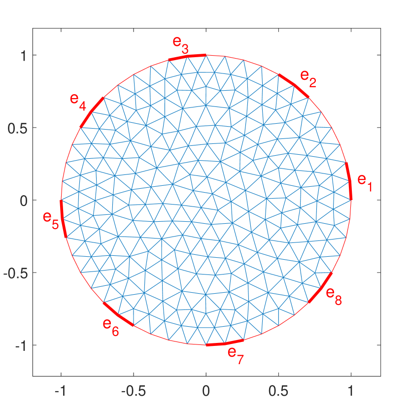
Figure 1: left: Electrodes (in red) on the boundary with $L=4$; right: finite element discretization with $8$ electrodes

Let $J_{i}$, $E_{i}$, $i=1,2,\dots,I$, be the current density and the electric field in the $i$th measurement, and let $\phi_{i}$, $\psi_{i}$ be the potentials for $J_{i}$, $E_{i}$; then they must satisfy

$$\sqrt{\sigma}\nabla\phi_{i}-\frac{1}{\sqrt{\sigma}}\nabla^{\bot}\psi_{i}=0 \quad\text{in \;}\Omega,$$ (57a)

$$\phi_{i}+z_{\ell}\nabla^{\bot}\psi_{i}\cdot\nu=v_{\ell,i} \quad\text{on \;}e_{\ell},\ell=1,2,\dots,L,$$ (57b)

$$\int_{e_{\ell}}\nabla^{\bot}\psi_{i}\cdot\nu{~{}\mathrm{d}}s=j_{\ell,i} \quad\text{for \;}\ell=1,2,\dots,L,$$ (57c)

$$\nabla^{\bot}\psi_{i}\cdot\nu=0 \quad\text{on \;}\partial\Omega\backslash\cup_{\ell=1}^{L}e_{\ell},$$ (57d)

$\forall i=1,2,\dots,I$, where

• $j_{\ell,i}$, $v_{\ell,i}$ are the applied current and measured voltage on $e_{\ell}$ at the $i$th measurement,

• $\{z_{\ell}\}_{\ell=1}^{L}$ is the set of positive contact impedances.

By assuming $\psi(e_{i}^{a})=0$ and using (57c), (57d) (57b), we get

$$\psi_{i}|_{g_{\ell}}=\bar{j}_{\ell,i}, \quad\forall\ell\in\{1,\dots,L\},$$

$$\int_{e_{\ell}^{a}}^{x}\phi_{i}{~{}\mathrm{d}}s-z_{\ell}\psi_{i}(x)=\bar{v}_{\ell,i}(x), \quad\forall x\in e_{\ell},\forall\ell\in\{1,\dots,L\},$$

where $\bar{j}_{\ell,i}=-\sum_{k=1}^{\ell}j_{k,i}$, $\bar{v}_{\ell,i}(x)=-z_{\ell}\Big{(}-\sum_{k=1}^{\ell-1}j_{k,i}\Big{)}+v_{\ell,i}d_{e_{\ell}}(x)$ and $d_{e_{\ell}}(x)$ is the length of $e_{\ell}$ from $e_{\ell}^{a}$ to $x$.

In the case of EIT, the data $(j_{\ell,i},v_{\ell,i})_{\ell,i}\in\mathbb{R}^{2LI}$ can be considered as $(\bar{j}_{\ell,i},\bar{v}_{\ell,i})_{\ell,i}\in\prod_{i=1}^{I}\prod_{\ell=1}^{L}(L^{2}(g_{\ell})\times L^{2}(e_{\ell}))$ and the cost function part corresponding to observations is chosen as $J^{EIT}_{obs}:H^{1}(\Omega)^{2I}\to\mathbb{R}$,

$$J^{EIT}_{obs}(\Phi,\Psi;\bar{j},\bar{v})=\frac{1}{2}\sum_{i=1}^{I}\sum_{\ell=1}^{L}\Big{(}\int_{g_{\ell}}|\psi_{i}-\bar{j}_{\ell,i}|^{2}{~{}\mathrm{d}}s+\int_{e_{\ell}}\Big{|}\int\phi_{i}|_{e_{\ell}}-z_{\ell}\psi_{i}-\bar{v}_{\ell,i}\Big{|}^{2}{~{}\mathrm{d}}s\Big{)},$$ (58)

where $\Phi=(\phi_{i})_{i}$, $\Psi=(\psi_{i})_{i}$, $\bar{j}=(\bar{j}_{\ell,i})_{\ell,i}$, $\bar{v}=(\bar{v}_{\ell,i})_{\ell,i}$ and $\int\phi_{i}|_{e_{\ell}}:e_{\ell}\to\mathbb{R},x\mapsto\int_{e_{\ell}^{a}}^{x}\phi_{i}{~{}\mathrm{d}}s$.

In the case of IAT, instead of $(j_{\ell,i},v_{\ell,i})_{\ell,i}$, we observe $\mathcal{H}=(\mathcal{H}_{i})_{i}=(\sigma|\nabla\phi_{i}|^{2})_{i}$ and the cost function part corresponding to these observations is $J^{IAT}_{obs}:L^{2}(\Omega)\times H^{1}(\Omega)^{I}\to\mathbb{R}$,

$$J^{IAT}_{obs}(\sigma,\Phi;\mathcal{H})=\frac{1}{2}\sum_{i=1}^{I}\int_{\Omega}\Big{|}\sigma|\nabla\phi_{i}|^{2}-\mathcal{H}_{i}\Big{|}^{2}{~{}\mathrm{d}}\Omega.$$ (59)

In both cases of EIT and IAT, we choose the cost function part corresponding to the model as $J^{KV}_{mod}:L^{2}(\Omega)\times H^{1}(\Omega)^{2I}\to\mathbb{R}$,

$$J^{KV}_{mod}(\sigma,\Phi,\Psi)=\frac{1}{2}\sum_{i=1}^{I}\int_{\Omega}\Big{|}\sqrt{\sigma}\nabla\phi_{i}-\frac{1}{\sqrt{\sigma}}\nabla^{\bot}\psi_{i}\Big{|}^{2}{~{}\mathrm{d}}\Omega$$ (60)

and combine it with the model part to

$$J^{IAT}(\sigma,\Phi,\Psi)=J^{KV}_{mod}(\sigma,\Phi,\Psi)+J^{IAT}_{obs}(\sigma,\Phi;\mathcal{H})$$ (61)

$$J^{EIT}(\sigma,\Phi,\Psi)=J^{KV}_{mod}(\sigma,\Phi,\Psi)+J^{EIT}_{obs}(\Phi,\Psi;\bar{j},\bar{v})$$ (62)

on the admissible sets

$$M^{IAT}_{{\mathrm{ad}}}=M^{EIT}_{{\mathrm{ad}}}=L^{2}_{[\underline{\sigma},\overline{\sigma}]}(\Omega)\times H_{\diamondsuit}^{1}(\Omega)\times H_{0}^{1}(\Omega)+\Phi_{0}$$

As in the previous section, besides the resulting all-at-once versions (cf. EIT (i), (ii) and IAT (i)) we also consider some of the reduced versions of the cost function.

The first version involves eliminating $\sigma$ from the cost function (cf. EIT (iii), (iv) and IAT (ii)), by defining, for given $\Phi,\Psi$, the corresponding $\sigma$ by

$$\begin{split}\sigma(\Phi,\Psi)&=\operatorname*{argmin}_{\sigma}\Big{\{}\frac{1}{2}\sum_{i=1}^{I}\int_{\Omega}\Big{|}\sqrt{\sigma}\nabla\phi_{i}-\frac{1}{\sqrt{\sigma}}\nabla^{\bot}\psi_{i}\Big{|}^{2}{~{}\mathrm{d}}\Omega:\sigma\in L^{2}_{[\underline{\sigma},\overline{\sigma}]}(\Omega)\Big{\}}\\ &=\operatorname*{argmin}_{\sigma}\Big{\{}\sum_{i=1}^{I}\int_{\Omega}\Big{(}\sigma|\nabla\phi_{i}|^{2}+\frac{1}{\sigma}|\nabla^{\bot}\psi_{i}|^{2}\Big{)}{~{}\mathrm{d}}\Omega:\sigma\in L^{2}_{[\underline{\sigma},\overline{\sigma}]}(\Omega)\Big{\}}\end{split}$$ (63)

or explicitly

$$\begin{split}\sigma(\Phi,\Psi)&=\min\Bigg{\{}\overline{\sigma},\max\Bigg{\{}\underline{\sigma},\sqrt{\frac{\sum_{i=1}^{I}|\nabla^{\bot}\psi_{i}|^{2}}{\sum_{i=1}^{I}|\nabla\phi_{i}|^{2}}}\Bigg{\}}\Bigg{\}}.\end{split}$$

For the case of IAT, we set

$$\begin{split}J^{IAT}_{\sigma}(\Phi,\Psi;\mathcal{H})&=J^{KV}_{mod}(\sigma(\Phi,\Psi),\Phi,\Psi)+\beta J^{IAT}_{obs}(\sigma(\Phi,\Psi),\Phi;H)\end{split}$$ (64)

for the case of EIT,

$$\begin{split}J^{EIT}_{\sigma}(\Phi,\Psi;\bar{j},\bar{v})&=J^{KV}_{mod}(\sigma(\Phi,\Psi),\Phi,\Psi)+\beta J^{EIT}_{obs}(\Phi,\Psi;\bar{j},\bar{v})\end{split}$$ (65)

and in both cases

$$M^{IAT}_{\sigma,{\mathrm{ad}}}=M^{EIT}_{\sigma,{\mathrm{ad}}}=H_{\diamondsuit}^{1}(\Omega)\times H_{0}^{1}(\Omega)+\Phi_{0}\,.$$

Note that in spite of the minimizing pre-definition of $\sigma(\Phi,\Psi)$, the model cost function part may be nonzero due to the constraints and therefore still needs to be taken into account.

The second alternative cost function involves eliminating $(\Phi,\Psi)$ from the cost function (cf. EIT (v), (vi) and IAT (iii)) by means of the weak form of the CEM PDE (57)

$$\begin{split}&\int_{\Omega}\sigma\nabla\phi_{i}\cdot\nabla p{~{}\mathrm{d}}\Omega+\sum_{\ell=1}^{L}\frac{1}{z_{\ell}}\int_{e_{\ell}}(\phi_{i}-v_{\ell,i})(p-\xi_{\ell}){~{}\mathrm{d}}s=\sum_{\ell=1}^{L}j_{\ell,i}\xi_{\ell},\forall(p,\xi)\in H^{1}(\Omega)\times\mathbb{R}^{L},\end{split}$$ (66)

and $\nabla^{\bot}\psi_{i}=\sigma\nabla\phi_{i},\forall i\in\{1,\dots,I\}$, which leads to $J^{KV}_{mod}(\sigma,\Phi(\sigma),\Psi(\sigma))=0$. Hence, we have, for the case of IAT,

$$\begin{split}J^{IAT}_{(\Phi,\Psi)}(\sigma;\mathcal{H})&=J^{IAT}_{obs}(\sigma,\Phi(\sigma);\mathcal{H})=\frac{1}{2}\sum_{i=1}^{I}\int_{\Omega}\Big{(}\sigma|\nabla\phi_{i}(\sigma)|^{2}-\mathcal{H}_{i}\Big{)}^{2}{~{}\mathrm{d}}\Omega;\end{split}$$ (67)

for the case of EIT,

$$\begin{split}J^{EIT}_{(\Phi,\Psi)}(\sigma;v)&=\frac{1}{2}\sum_{i=1}^{I}\sum_{\ell=1}^{L}\big{|}v_{\ell,i}(\sigma)-v_{\ell,i}\big{|}^{2},\end{split}$$ (68)

where, $v(\sigma)=(v_{\ell,i}(\sigma))_{i\in\{1,\dots,I\},\ell\in\{1,\dots,L\}}$ is the solution to (66) and

$$M^{IAT}_{(\Phi,\Psi),{\mathrm{ad}}}=M^{EIT}_{(\Phi,\Psi),{\mathrm{ad}}}=L^{2}_{[\underline{\sigma},\overline{\sigma}]}(\Omega)$$

5.2 Implementation using the finite method in Matlab

In order to generate synthetic data by solving the CEM PDE (57) using the finite element method. In all aour computations, $\Omega$ is the unit circle in $\mathbb{R}^{2}$ with eight identical electrodes ($L=8$) denoted by $e_{1},\dots,e_{8}$ attached equidistantly on its boundary (see Figure 1). The domain $\Omega$ is decomposed by a regular finite element mesh defined by nodes $P_{k},k\in\{1,\dots,N_{\mathrm{node}}=913\}$ and elements $\Omega_{h},h\in\{1,\dots,N_{\mathrm{element}}=432\}$ and the ansatz spaces $L^{2}(\Omega)$ for $\sigma$ and $H^{1}(\Omega)$ for $\phi,\psi$ are approximated by piecewise constant and continuous piecewise quadratic finite elements spaces $\tilde{L}^{2}(\Omega)$ and $\tilde{H}^{1}(\Omega)$, respectvely.

With $L=8$ electrodes, there are $N_{\mathrm{meas}}=28$ possible combinations of excitations – we will use some of them to reconstruct $\sigma$ later. At the $i$th measurement, we impose the injected current $Jsigma_{I}=(j_{\ell,i})_{\ell=1}^{L}$ with

$$\left\{\begin{array}[]{ll}j_{\ell_{1},i}=1,j_{\ell_{2},i}=-1,&\text{\, if $\ell_{1}<\ell_{2}$ and $\{\ell_{1},\ell_{2}\}$ is the $i$th element of}\\ &\text{\, the family of 2-elements subsets of $\{1,\dots,8\}$},\\ j_{\ell,i}=0,&\text{\, otherwise,}\end{array}\right.$$

at the electrodes and then solve the Galerkin discretized weak form (cf. (66))

$$\begin{split}\int_{\Omega}\sigma^{\mathrm{ex}}\nabla\phi_{i}\cdot\nabla p{~{}\mathrm{d}}x+\sum_{\ell=1}^{L}\frac{1}{z_{\ell}}\int_{e_{\ell}}(\phi_{i}-v_{\ell,i})(p-\xi_{\ell}){~{}\mathrm{d}}s=\sum_{\ell=1}^{L}j_{\ell,i}\xi_{\ell},\\ \forall(p,\xi)\in\tilde{H}^{1}(\Omega)\times\mathbb{R}^{L},\forall i\in\{1,\dots,N_{\mathrm{meas}}\}\end{split}$$ (69)

to find $(\phi^{\mathrm{ex}}_{i},(v^{\mathrm{ex}}_{\ell,i}))$ and the corresponding exact data

$$\mathcal{H}^{\mathrm{ex}}=(\sigma^{\mathrm{ex}}|\nabla\phi^{\mathrm{ex}}_{1}|^{2},\dots,\sigma^{\mathrm{ex}}|\nabla\phi^{\mathrm{ex}}_{N_{\mathrm{meas}}}|^{2})\mbox{ for IAT;}\quad(j_{\ell,i},v^{\mathrm{ex}}_{\ell,i})_{\ell,i}\mbox{ for EIT.}$$

The synthetic measured data is generated by adding random noise such that

$$|\mathcal{H}^{\delta}_{i}-\mathcal{H}^{\mathrm{ex}}_{i}|\leq\delta|\mathcal{H}^{\mathrm{ex}}_{i}|,\ \forall i\mbox{ for IAT;}\quad|v^{\delta}_{\ell,i}-v^{\mathrm{ex}}_{\ell,i}|\leq\delta|v^{ex}_{\ell,i}|\mbox{ for EIT,}$$

which in an obvious way defines the noisy versions $J^{\delta}$, $J_{\sigma}^{\delta}$, $J_{\Phi,\Psi}^{\delta}$ and $M^{\delta}$, $M_{\sigma,{\mathrm{ad}}}^{\delta}$, $M_{(\Phi,\Psi),{\mathrm{ad}}}^{\delta}$ of the cost functions and admissible sets, respectively. In our tests we consider three values of $\delta$: $\delta=0$, $\delta=0.01$ and $\delta=0.1$.

To avoid an inverse crime, we used a coarser mesh in our reconstructions.

In (66) we set the value of contact impedances $z_{\ell}$, $\ell\in\{1,\dots,L\}$, to 0.1.

The test case considered in all of our computational results is defined by a constant inclusion on a constant background

$$\sigma^{{\mathrm{ex}}}(x)=\left\{\begin{array}[]{ll}5,&\text{\; in \;}\Omega_{h}\text{\; if \;}\Omega_{h}\subset B_{0.5}(-0.3,-0.1)\\ 2,&\text{\; otherwise,}\end{array}\right.$$

where $B_{r}(p_{1},p_{2})\subset\mathbb{R}^{2}$ is the ball centered at $(p_{1},p_{2})$ with radius $r$.

With each of the three above mentioned cost function combinations (all-at-once, eliminated $\sigma$, eliminated $(\Phi,\Psi)$, the iterates $x_{k}=(\sigma_{k},\Phi_{k},\Psi_{k})$, or $x_{k}=(\Phi_{k},\Psi_{k})$, or $x_{k}=\sigma_{k}$, are defined by the projected gradient method (12) from Section 2 where $\mu_{k}$ is found by an Armijo back tracking line search. Details on computation of the gradients of the various cost functions can be found in [8]. The iteration is stopped by the discrepancy principle (20) in the noisy case and as soon as the step size fell below a value $\epsilon_{\mu}$ (which we set to $10^{10}$ in our tests) in case of exact data.

5.3 Numerical results for IAT

We consider four cases of excitations, namely

• $I=1$, with $j_{1,1}=1$, $j_{5,1}=-1$ and $j_{k,1}=0$ otherwise;

• $I=2$, with $j_{1,1}=j_{3,2}=1$, $j_{5,1}=j_{7,2}=-1$, and $j_{k,i}=0$ otherwise;

• $I=4$, with $j_{1,1}=j_{3,2}=j_{2,3}=j_{4,4}=1$, $j_{5,1}=j_{7,2}=j_{6,3}=j_{8,4}=-1$ and $j_{k,i}=0$ otherwise.

• $I=28$, with all $({8\atop 2})$ combinations of setting $j_{k,i}=1$, $j_{\ell,i}=-1$ for $k\not=\ell\in\{1,\ldots,8\}$

The starting value is set to the mean value of the maximal and minimal value for the conductivity $\sigma_{0}=\frac{1}{2}(\underline{\sigma}+\overline{\sigma})$ and $\Phi_{0},\Psi_{0}$, if necessary, are gained from the weak form (66) where $\sigma$ is replaced by $\sigma_{0}$.

The tables below show the data about the number of iterations, the error $\|\sigma_{end}-\sigma^{{\mathrm{ex}}}\|_{L^{2}(\Omega)}$, the CPU time (in seconds) and the CPU time for each iteration for various versions of cost functions.

all-at-once version		number	$L^{2}$ error	CPU-time	CPU-time
IAT		of iterations	$\|\sigma_{end}-\sigma^{{\mathrm{ex}}}\|$	(in seconds)	per iteration
$I=1$	$\delta=0$	5 025 130	0.658 72	943 527	0.187 76
	$\delta=0.01$	4 959 452	0.665 37	930 984	0.187 72
	$\delta=0.1$	5 178 542	0.806 76	984 851	0.190 18
$I=2$	$\delta=0$	1 109 245	0.387 57	266 270	0.240 05
	$\delta=0.01$	1 114 829	0.387 46	264 697	0.237 43
	$\delta=0.1$	1 520 239	0.567 00	344 894	0.226 87
$I=4$	$\delta=0$	301 651	0.310 70	73 664	0.244 20
	$\delta=0.01$	308 170	0.314 96	74 474	0.241 66
	$\delta=0.1$	326 561	0.412 61	79 693	0.244 04
$I=28$	$\delta=0$	249 816	0.305 35	82 681	0.330 97
	$\delta=0.01$	245 306	0.306 75	81 263	0.331 27
	$\delta=0.1$	292 914	0.326 76	96 378	0.329 03

Table 1: IAT, all-at-once version (60), (59).

eliminating-$\sigma$		number	$L^{2}$ error	CPU-time	CPU-time
version, IAT		of iterations	$\|\sigma_{end}-\sigma^{{\mathrm{ex}}}\|$	(in seconds)	per iteration
$I=1$	$\delta=0$	2 224	0.582 89	583	0.262 28
	$\delta=0.01$	1 230	0.797 77	319	0.259 46
	$\delta=0.1$	840	0.944 67	215	0.256 36
$I=2$	$\delta=0$	3 488	0.360 50	1 232	0.353 21
	$\delta=0.01$	2 894	0.373 53	920	0.317 86
	$\delta=0.1$	2 645	0.455 20	959	0.362 74
$I=4$	$\delta=0$	2 730	0.324 27	801	0.293 49
	$\delta=0.01$	3 393	0.321 52	1 254	0.369 59
	$\delta=0.1$	1 836	0.433 52	562	0.305 89
$I=28$	$\delta=0$	3 330	0.330 32	1 451	0.435 61
	$\delta=0.01$	3 251	0.331 05	1 427	0.439 00
	$\delta=0.1$	3 300	0.344 39	1 511	0.457 87

Table 2: IAT, eliminating-$\sigma$ version (64).

eliminating-$(\Phi,\Psi)$		number	$L^{2}$ error	CPU-time	CPU-time
version, IAT		of iterations	$\|\sigma_{end}-\sigma^{{\mathrm{ex}}}\|$	(in seconds)	per iteration
$I=1$	$\delta=0$	225 302	2.73e-09	147 936	0.656 61
	$\delta=0.01$	100 041	0.018 45	83 302	0.832 68
	$\delta=0.1$	79 377	0.224 34	38 043	0.479 27
$I=2$	$\delta=0$	55 066	1.68e-10	30 161	0.547 72
	$\delta=0.01$	61 162	0.016 69	61 202	1.000 65
	$\delta=0.1$	38 162	0.174 07	41 314	1.082 60
$I=4$	$\delta=0$	13 782	4.38e-11	10 469	0.759 58
	$\delta=0.01$	19 889	0.014 41	27 064	1.360 76
	$\delta=0.1$	15 169	0.122 03	19 721	1.300 06
$I=28$	$\delta=0$	13 868	4.38e-11	49 005	3.533 65
	$\delta=0.01$	23 540	0.007 44	96 096	4.082 26
	$\delta=0.1$	28 721	0.067 32	120 978	4.212 17

Table 3: IAT, eliminating-$(\Phi,\Psi)$ version (67).

Finally, in Figures 2, 3 and 4, we display some pictures of reconstructions.

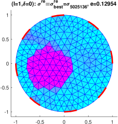
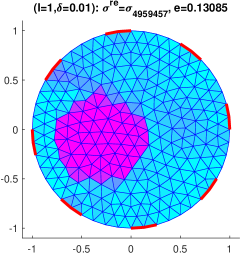
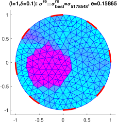
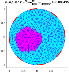
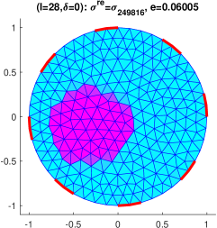
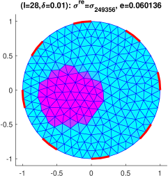
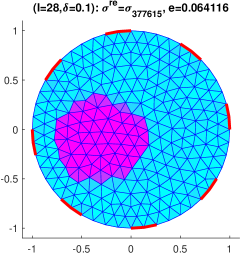
Figure 2: Reconstructions of $\sigma$ from all-at-once version of cost function IAT (60), (59), in cases $I=1$, $I=2$, $I=4$, $I=28$ (top to bottom) for $\delta=0$, $\delta=0.01$, $\delta=0.1$ (left to right).

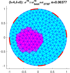
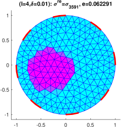
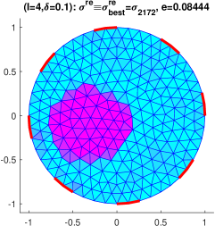
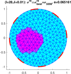
Figure 3: Reconstructions of $\sigma$ from eliminating-$\sigma$ version of cost function IAT (64), in cases $I=1$, $I=2$, $I=4$, $I=28$ (top to bottom) for $\delta=0$, $\delta=0.01$, $\delta=0.1$ (left to right).

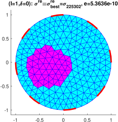
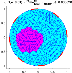
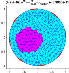
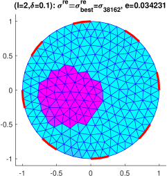
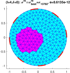
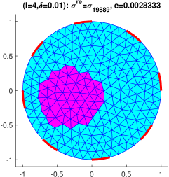
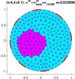
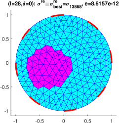
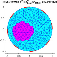
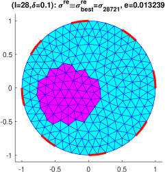
Figure 4: Reconstructions of $\sigma$ from eliminating-$\Phi-\Psi$ version of cost function IAT (67), in cases $I=1$, $I=2$, $I=4$, $I=28$ (top to bottom) for $\delta=0$, $\delta=0.01$, $\delta=0.1$ (left to right).

5.4 Numerical results for EIT

We close with a few pictures of reconstructions for EIT. Here, for obvious identifiabilty reasons, it is necessary to use all measurements $I=28$. Moreover, the all-at-once and eliminating-$\sigma$ versions failed to converge, so we here only provide results with the classical reduced version of EIT corresponding to (68). Starting from the constant value $\sigma_{0}=\frac{1}{2}\big{(}\underline{\sigma}+\overline{\sigma}\big{)}$ we obtain the reconstructions in Figure 5 for noise levels of zero, one and ten per cent. Note that in view of the exponential ill-posedness of this inverse problem, the quality of reconstructions is more than reasonable for this level of data contamination.

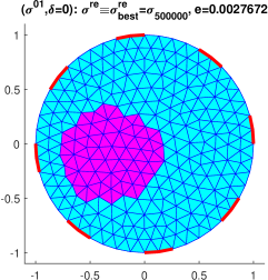
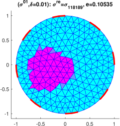
Figure 5: Reconstructions of $\sigma$ from eliminating-$(\Phi,\Psi)$ version of cost function EIT (68), in case $I=28$, $\delta=0$, $\delta=0.01$, $\delta=0.1$ (left to right)..

More details in particular on numerical tests for EIT can be found in the PhD thesis [8].

6 Conclusions and remarks

In this paper we have provided convergence results on the iterative solution methods (gradient or Newton type) for minimization based formulations of inverse problems. We apply these to the identification of a spatially varying diffusion coefficient in an elliptic PDE from different kinds of measurements, in particular corresponding to the electrical impedance tomography EIT and the impedance acoustic tomography IAT problem, for which we also provide numerical tests. Future work will, e.g., be concerned with investigations on the convexity conditions: How can an additive combination of functionals and constraints help to satisfy them, e.g., for EIT or IAT?

Appendix

Lemma 6.1

(Opial, discrete) Let $S$ be a non empty subset of a Hilbert space $X$, and $(x_{k})_{k\in\mathbb{N}}$ a sequence of elements of $X$. Assume that

1. for every $z\in S$, $\lim_{k\to\infty}\|x_{k}-z\|$ exists;

2. every weak sequential limit point of $(x_{k})_{k\in\mathbb{N}}$, as $k\to\infty$, belongs to $S$.

Then $x_{k}$ converges weakly as $k\to\infty$ to a point in $S$.

Lemma 6.2

(Opial, continuous) Let $S$ be a non empty subset of a Hilbert space $X$, and $x:[0,\infty)\to X$ a map. Assume that

1. for every $z\in S$, $\lim_{t\to\infty}\|x(t)-z\|$ exists;

2. every weak sequential limit point of $x(t)$, as $t\to\infty$, belongs to $S$.

Then $x(t)$ converges weakly as $t\to\infty$ to a point in $S$.

References

• [1] Bakushinskii, A.B.: The problem of the convergence of the iteratively regularized Gauss-Newton method. Comput. Math. Math. Phys. 32, 1353–1359 (1992)
• [2] Bakushinsky, A.B., Kokurin, M.Y.: Iterative Methods for Approximate Solution of Inverse Problems, Mathematics and Its Applications, vol. 577. Springer, Dordrecht (2004)
• [3] Boţ, R.I., Hein, T.: Iterative regularization with a general penalty term—theory and application to $L^{1}$ and $TV$ regularization. Inverse Problems 28(10), 104010, 19 (2012). DOI 10.1088/0266-5611/28/10/104010
• [4] Eicke, B.: Iteration methods for convexly constrained ill-posed problems in Hilbert space. Numerical Functional Analysis and Optimization 13(5–6), 413–429 (1992). DOI 10.1080/01630569208816489
• [5] Hanke, M.: A regularization Levenberg-Marquardt scheme, with applications to inverse groundwater filtration problems. Inverse Problems 13, 79–95 (1997)
• [6] Hanke, M., Neubauer, A., Scherzer, O.: A convergence analysis of the Landweber iteration for nonlinear ill-posed problems. Numer. Math. 72, 21–37 (1995)
• [7] Hanke, M., Scherzer, O.: Inverse problems light: Numerical differentiation. American Mathematical Monthly 108 (2001). DOI 10.2307/2695705
• [8] Huynh, K.V.: Solving inverse problems without forward operators: Application examples and iterative solvers. Ph.D. thesis, Alpen-Adria-Universität Klagenfurt (2021)
• [9] Jin, Q., Wang, W.: Landweber iteration of Kaczmarz type with general non-smooth convex penalty functionals. Inverse Problems 29(8), 085011, 22 (2013). DOI 10.1088/0266-5611/29/8/085011
• [10] Kaltenbacher, B.: Regularization based on all-at-once formulations for inverse problems. SIAM Journal on Numerical Analysis 54, 2594–2618 (2016). DOI doi.org/10.1137/16M1060984. ArXiv:1603.05332v1 [math.NA]
• [11] Kaltenbacher, B.: All-at-once versus reduced iterative methods for time dependent inverse problems. Inverse Problems 33, 064002 (2017). DOI 10.1088/1361-6420/aa6f34. Arxiv: 1910.02857 [math.NA]
• [12] Kaltenbacher, B.: Minimization based formulations of inverse problems and their regularization. SIAM Journal on Optimization 28, 620–645 (2018). DOI 10.1137/17M1124036
• [13] Kaltenbacher, B., Klassen, A., Previatti de Souza, M.: The Ivanov regularized Gauss-Newton method in Banach space with an a posteriori choice of the regularization radius. Journal of Inverse and Ill-posed Problems 27, 539–557 (2019). DOI 10.1515/jiip-2018-0093. Arxiv:1910.01811 [math.NA]
• [14] Kaltenbacher, B., Neubauer, A.: Convergence of projected iterative regularization methods for nonlinear problems with smooth solutions. Inverse Problems 22, 1105–1119 (2006)
• [15] Kaltenbacher, B., Neubauer, A., Scherzer, O.: Iterative Regularization Methods for Nonlinear Problems. de Gruyter, Berlin, New York (2008). Radon Series on Computational and Applied Mathematics
• [16] Kaltenbacher, B., Nguyen, T.T.N., Scherzer, O.: The tangential cone condition for some coefficient identification model problems in parabolic PDEs. In: B. Kaltenbacher, A. Wald, T. Schuster (eds.) Time-dependent Problems in Imaging and Parameter Identification. Springer (2020). To appear
• [17] Kaltenbacher, B., Schöpfer, F., Schuster, T.: Convergence of some iterative methods for the regularization of nonlinear ill-posed problems in Banach spaces. Inverse Problems 25 (2009). 065003 doi: 10.1088/0266-5611/25/6/065003
• [18] Kaltenbacher, B., Previatti de Souza, M.: Convergence and adaptive discretization of the IRGNM Tikhonov and the IRGNM Ivanov method under a tangential cone condition in Banach space. Numerische Mathematik 140, 449–478 (2018). DOI 10.1007/s00211-018-0971-5. Arxiv:1707.07589 [math.NA]
• [19] Kindermann, S.: Convergence of the gradient method for ill-posed problems. Inv. Probl. Imaging 11(4), 703–720 (2017). DOI 10.3934/ipi.2017033
• [20] Kohn, R.V., Vogelius, M.: Relaxation of a variational method for impedance computed tomography. Communications on Pure and Applied Mathematics 40(6), 745–777 (1987)
• [21] Van Huynh, K., Kaltenbacher, B.: Some application examples of minimization based formulations of inverse problems and their regularization. Inverse Problems and Imaging (2020). DOI 10.3934/ipi.2020074. ArXiv:2004.12965 [math.NA]
• [22] Wang, J., Wang, W., Han, B.: An iteration regularization method with general convex penalty for nonlinear inverse problems in banach spaces. Journal of Computational and Applied Mathematics 361, 472 – 486 (2019). DOI https://doi.org/10.1016/j.cam.2019.05.008
• [23] Widlak, T., Scherzer, O.: Hybrid tomography for conductivity imaging. Inverse Problems 28(8), 084008 (2012). DOI 10.1088/0266-5611/28/8/084008