Understanding the Role of Scene Graphs in Visual Question Answering

Abstract

Visual Question Answering (VQA) is of tremendous interest to the research community with important applications such as aiding visually impaired users and image-based search. In this work, we explore the use of scene graphs for solving the VQA task. We conduct experiments on the GQA dataset (Hudson and Manning, 2019b) which presents a challenging set of questions requiring counting, compositionality and advanced reasoning capability, and provides scene graphs for a large number of images. We adopt image + question architectures for use with scene graphs, evaluate various scene graph generation techniques for unseen images, propose a training curriculum to leverage human annotated and auto-generated scene graphs, and build late fusion architectures to learn from multiple image representations. We present a multi-faceted study into the use of scene graphs for VQA, making this work the first of its kind.

1 Introduction

The task of Visual Question Answering (VQA) requires a model to answer a free-form natural language question that is based on an image. It is an important Vision+Language (V+L) task that has numerous real-world applications such as image-based search, search and rescue missions, visually capable AI assistants and aiding visually impaired users. A number of VQA datasets such as VQA 2.0 (Antol et al., 2015), CLEVR (Johnson et al., 2017) and GQA (Hudson and Manning, 2019b) have been introduced, fuelling research in the area.

Research in VQA includes works that find biases in the data, demonstrating the need for improved datasets (Agrawal et al., 2018), pre-trained models such as lxmert (Tan and Bansal, 2019) and uniter (Chen et al., 2020) that beat the state of the art on a variety of V+L tasks and models such as neural module networks (Andreas et al., 2016) constructed to heighten interpretability, among many others. However, few works have explored the use of scene graphs for the VQA task. Scene graphs provide a graphical representation of the image, containing information about objects and relationships between them. This representation is more advantageous than the typical object features extracted from an image since it is in natural language and allows for greater interpretability. The recently released GQA dataset (Hudson and Manning, 2019b) contains 85,638 scene graphs for images in the training and validation sets, spurring research into the use of scene graphs for VQA.

In this work, we explore a set of research questions related to the use of scene graphs for VQA. Given the success of pre-trained models for other V+L tasks, we evaluate the effectiveness of transfer learning for GQA. The use of scene graphs requires converting them from a graphical representation to one that can be undeerstood by a neural network. We adopt the popular Graph Network model (Battaglia et al., 2018) to produce scene graph encodings and then adopt image-based question answering models to use these encodings. One of the challenges in using scene graphs lies in generating them for unseen images. We compare multiple scene graph generation models and study the impact of scene graph quality on model performance. We devise a novel training curriculum aimed at leveraging both ground truth and generated scene graphs to avoid a mismatch between training and testing scene graphs. Additionally, we explore late-fusion ensembles with the goal of using images as well as scene graphs, and combining the strengths of scene graph use with those of pre-training. We present the first in-depth analysis of the use of scene graphs for VQA. We will release our source code, end-to-end pipelines and pre-trained checkpoints in our GitHub repository.

The remainder of this paper is structured as follows. In Section 2 we introduce existing approaches to VQA and formally define our task in Section 3. We describe our methodology and experimental setup in Section 4 and 5 respectively. In Section 6, we provide an in-depth analysis of our results. We conclude the paper with a summary of our contributions in Section 7.

2 Related Work

In this section we discuss VQA datasets, state of the art approaches for VQA, usage of scene graphs, and methods of scene graph generation.

2.1 Datasets for VQA

Antol et al. (2015) released the VQA 2.0 dataset containing 204,721 real images and 1,105,904 open-ended questions requiring open-ended or multiple-choice answers. Prior works have identified statistical biases in VQA 2.0 with educated guess approaches working remarkably well. The CLEVR dataset (Johnson et al., 2017) was introduced with the goal of mitigating these biases and testing the visual reasoning capability of models using a large number of compositional questions. However, the number of objects in CLEVR is severely limited and the number of possible answers is just 28. Moreover, the images are synthetically generated. In this work, we conduct experiments on the GQA dataset (Hudson and Manning, 2019b) which contains few statistical biases, retains the semantic richness of real images, contains open-ended questions of various degrees of compositionality and has a much larger vocabulary than CLEVR. Importantly for this work, it provides cleaned up versions of Visual Genome scene graphs (Krishna et al., 2017) for images in the training and validation sets.

2.2 Approaches to VQA

With the introduction of the VQA 2.0 and CLEVR datasets, many models have been proposed for the VQA task. This section covers some task specific and pre-trained models, each of which have beaten prior state of the art approaches for VQA.

2.2.1 Task Specific Models

We classify the set of models trained from scratch for a specific task on a single dataset as task specific. While the performance of these models may not match that of models which leverage transfer learning, they present interesting architectures that can be modified to use scene graphs. We discuss two such models here.
Bottom-Up Top-Down Attention (BUTD): Anderson et al. (2018) propose a combined bottom-up and top-down mechanism for vision and language representation learning. For VQA, top-down attention uses the question, usually predicting an attention distribution over a uniform grid of equally-sized image regions. In contrast, bottom-up attention proposes a set of salient image regions using Faster R-CNN (Ren et al., 2016), which can be attended on. This architecture has proven beneficial for VQA and image captioning.
MAC: Hudson and Manning (2018) introduce a neural network architecture that decomposes a question answering task into a series of attention-based reasoning steps, thus increasing the interpretability of the model’s decision making process. Given a knowledge-base $K$ (image) and a task description $Q$ (question), the control unit (cu) of the model identifies a series of operations to be performed, the read unit (ru) extracts information needed to perform the operation from the image, and the write unit (wu) integrates the information into an internal cell state to produce an intermediate result. The mac model is one of the baselines introduced with the GQA dataset. Since, it is not a pre-trained model, it can easily be extended to use different knowledge bases without the additional overhead of pre-training.

2.2.2 Pre-Trained Models

In recent times, the introduction of pre-trained models such as BERT (Devlin et al., 2019) has advanced the state of the art on a number of Natural Language Processing tasks. Similar benefits of using Transfer Learning have been seen for vision based tasks. Thus, it is not surprising that pre-training has also had a huge impact on the performance on several Vision + Language tasks. Chen et al. (2020) try to learn a UNiversal Image-TExt Representation (uniter) through large-scale pre-training over four image + text datasets. To this end, they design four pre-training tasks: Masked Language Modeling, Masked Region Modeling, ImageText Matching and Word-Region Alignment. uniter achieves state of the art performance on challenges like VQA 2.0 and NLVR2, beating pre-trained models like lxmert (Tan and Bansal, 2019) and task-specific models like mac.

2.3 Using Scene Graphs for VQA

To the best of our knowledge, only a few prior works have used scene graphs for VQA. Hudson and Manning (2019b) report a validation set accuracy of 83.5 using a “perfect sight” mac which replaces object features with a representation of the scene graph. The exact details of the scene graph encoding are unclear. Lee et al. (2019) introduce another perfect sight model where the encoding of the scene graph is learnt using a Graph Network and is passed in place of the image to mac. Their model obtains a validation accuracy of 96.3 using ground truth scene graphs. Hudson and Manning (2019a) propose the task-specific Neural State Machine (NSM) which generates a probabilistic scene graph for the image and performs a series of reasoning operations over it. The generated scene graph contains a probability distribution for predicted objects, attributes, and relations. This allows the model to make predictions despite errors in the graph. While NSM gets a high accuracy, the lack of an open-source implementation and missing details required for reproducibility make comparisons with this model difficult.

2.4 Using scene graphs for other tasks

Scene graphs have proven to be useful in various domains of computer vision and visual understanding. Johnson et al. (2018) studied the role of scene graphs in generating images using natural language descriptions. In the field of image outpainting, the work by Li et al. (2019) has shown that the use of scene graphs produces much more effective visual results and quantitative evaluations. Lee et al. (2020) proposes a unique Neural Design Network that uses scene graphs to great effect in the context of layout generation. The effectiveness of scene graphs displayed in these fields further motivates the need to understand the impact of scene graphs in the domain of visual question answering.

2.5 Scene Graph Generation

The task of Scene Graph Generation has become an increasingly sought out challenge after discovering its potential to surpass the limits on visual reasoning and question answering tasks. Most works in scene graph generation rely on pre-trained object feature extractors like Faster-RCNN (Ren et al., 2016) and Mask-RCNN (He et al., 2017) to capture the object and attribute properties in the image. One of the earlier works in the field of scene graph generation, by Zellers et al. (2018) first introduced the concept of eliminating bias in the global context of determining relations with regards to relational edges. Xu et al. (2017) first aimed to solve the task of scene graph generation using standard RNNs which learns to iteratively improve its predictions via message passing. Another top performing model by Tang et al. (2019) constructs scene graphs in the form of tree structures (using TreeLSTMs) and performs very well on a plethora of visual reasoning tasks. The recent work by Tang et al. (2020) looks to generate unbiased scene graphs with more specific relations across edges by building causal graphs and uses counterfactual causality from the trained graph to infer the effect from bad bias.

3 Task Definition

In this work, we tackle the multimodal VQA task which involves answering a question $q$ given an image $I$. The question can be expressed as the sequence $(w_{1},w_{2},...,w_{n})$ where $w_{i}$ is a single word/token. We work with the following representations of the image:

• Spatial Feature: A single vector $S$ for the entire image

• Object Features: A set of $N^{v}$ vectors $O=(o_{1},o_{2},...,o_{N^{v}})$ representing $N^{v}$ objects in the image

• Scene Graph: A graphical representation $g$ of the contents of the image

We formally define the scene graph in Equation  (1), where $V$ is the set of nodes representing objects in the image, $E$ is the set of edges representing relations between objects, and $u$ is a global feature shared by all components of the graph. $N^{v}$ is the number of objects in the image, and $N^{e}$ is the number of relations. $v_{i}^{name}$ is the name of the object corresponding to the node $v_{i}$ and $v_{i}^{attr}$ is the set of attributes of the object. Similarly, $e_{j}^{name}$ is the name of the relation between a source object / node $e_{j}^{s}$ and a receiver object $e_{j}^{r}$.

$$\begin{gathered}g=(E,V,u)\\ V=(v_{1},v_{2},...,v_{N^{v}});v_{i}=(v_{i}^{name},v_{i}^{attr});\\ E=(e_{1},e_{2},...,e_{N^{e}});e_{j}=(e_{j}^{name},e_{j}^{s},e_{j}^{r});\\ e_{j}^{s},e_{j}^{r}\in V\end{gathered}$$ (1)

We work in a discriminative setting wherein, given $Q$ and one or more representations of $I$ as input, the model must select an answer for $Q$ from a fixed set of $n$ answers, A = ($A_{1}$, $A_{2}$, …, $A_{n}$).

4 Proposed Approach

In this section we present the details of our methodology.

4.1 Baselines

We define two multimodal baselines for VQA, one using the image spatial features $S$, namely the Concatenation Baseline (concat), and another using the image object features $O$, namely the Attention Baseline (attn). For all our baselines, we use mean pooled BERT embeddings $B$ of the question $q$. We also define unimodal baselines.

4.1.1 Multimodal Baselines

In the concat model, mean pooled representations of $O$ are passed in parallel with $B$ through two fully-connected layers with ReLU activation to get $b*1024$ vectors for both modalities, where $b$ is the batch size. These vectors are concatenated and passed through two fully-connected layers with ReLU activation in between.

In attn, we pass $B$ and $O$ through parallel fully-connected layers. We use the obtained question projection as the $query$ and the image projection as the $key$ & $value$ in an attention mechanism to attend over the objects. Here, we use an attention mask to deal with the variable number of objects in each image. We concatenate the output of the attention mechanism to the question representation. This is followed by a fully-connected layer, ReLU and a classifying layer to get a distribution over the answers. The model architecture is illustrated in Figure 1. Such attention-based techniques for multimodal-fusion have been used successfully in the past (Liang et al., 2019).

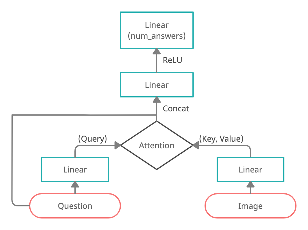
Figure 1: attn model architecture

4.1.2 Unimodal Baselines

For our unimodal baselines we remove the text component from the Concatenation Baseline to observe the impact of the image modality alone. Similarly, we remove the image component to observe the impact of the text modality alone.

4.2 UNITER

Given the state of the art performance achieved by the pre-trained uniter model on six different Vision + Language tasks, we use it to extract a cross-modal contextualized embedding $E$ for a given image and question. The embedding is passed through a multi-layer perceptron (mlp) which is trained during the process of fine-tuning uniter. The final layer of the mlp produces a softmax distribution over the answer set A, which is then used to predict an answer.

4.3 Scene Graph Encoding

Graph Neural Networks are a class of interpretable models successfully used for a range of tasks from relational reasoning to knowledge base completion (Zhou et al., 2018). Following the work of (Lee et al., 2019) we encode scene graphs using the class of graph neural networks introduced by Battaglia et al. (2018) - Graph Networks (GN).

As described in Equation 1, each node in the scene graph consists of a name and zero or more attributes. During pre-processing, we split the name and attributes into their constituent words, and represent a node with the vocabulary indices of these words. Similarly, an edge consists of the vocabulary indices of the relation name while the global vector is made up of the vocabulary indices of the question. These pre-processed representations are passed through a GloVe (Pennington et al., 2014) embedding layer followed by a single-layer bi-directional LSTM network to obtain the input graph representation for the Graph Network, $(E_{0},V_{0},u_{0})$. The Graph Network produces updated vectors following the algorithm described by (Zhou et al., 2018) which we show in Algorithm  1. Here, mlp refers to a multi-layer perceptron with two fully-connected layers of hidden size 512.

During iteration $t$, lines 2-4 update each edge using the value of the edge in iteration $t-1$, the node vectors for the source and receiver, and the global vector. Following the edge update, the nodes are updated in lines 5-9 using the updated values of incoming edges to the node, the previous node vector and the global vector. Finally, the global vector is updated (lines 10-14) using the updated values of all the nodes and edges. This process is repeated for 3 iterations with the output being updated edge, node and global vectors.

Precondition: Initial Graph $(E_{0},V_{0},u_{0})$

Postcondition: Encoding $(E_{T},V_{t},u_{T})$

1 for $t\in\{1...T\}$ do

2       for $k\in\{1...N^{e}\}$ do

3             $e_{k}^{{}^{\prime}}$ = mlp([$e_{k},v_{r_{k}},v_{s_{k}},u$])

4       end for

5      for $i\in\{1...N^{v}\}$ do

6             let $E_{i}^{{}^{\prime}}$ = ${(e_{k}^{{}^{\prime}},r_{k},s_{k})}_{r_{k}=i,k=1:N^{e}}$

7             $\bar{e}_{i}^{{}^{\prime}}$ = mean($E_{i}^{{}^{\prime}}$)

8             $v_{i}^{{}^{\prime}}$ = mlp([$\bar{e}_{i}^{{}^{\prime}}$, $v_{i},u$])

9            

10       end for

11      let $V^{{}^{\prime}}$ = $\{v^{{}^{\prime}}\}_{i=1:N^{v}}$

12       let $E^{{}^{\prime}}$ = $\{(e_{k}^{{}^{\prime}},r_{k},s_{k})\}_{k=1:N^{e}}$

13       $\bar{e}^{{}^{\prime}}$ = mean($E^{{}^{\prime}}$)

14       $\bar{v}^{{}^{\prime}}$ = mean($V^{{}^{\prime}}$)

15       $u^{{}^{\prime}}$ = mlp([$\bar{e}^{{}^{\prime}},\bar{v}^{{}^{\prime}},u$])

16       $(E,V,u)$ = $(E^{{}^{\prime}},V^{{}^{\prime}},u^{{}^{\prime}})$

17 end for

return $(E,V,U)$

Algorithm 1 Graph Network (GN)

4.4 Question Answering with Scene Graphs

As described in Section 4.3, the gn produces updated representations of the node, edge and global vectors. To convert these to a similar format as the object features $O$, we stack the node and global vectors to get the scene graph encoding, sge. The attn baseline (Section 4.1) takes as input, $O$. We replace this with sge to get a question answering model (sgatt) that uses scene graphs. Similarly, we pass sge to mac, replacing the image input, to get sgmac. We jointly train the gn and mac from scratch, and use gn weights thus obtained, to train sgatt.

4.5 Scene Graph Generation

The problem of generating a scene graph from an image is typically split into 2 phases. The first phase consists of training an object detector such as Faster-RCNN. The second phase uses the features extracted from this model to train a relation detector model responsible for identifying potential edge pairs between a set of objects and predicting the relationship between them. A popular work in the field of scene graph classification is the Neural Motifs (Zellers et al., 2018) model, which uses a stacked biLSTM structure to predict edge pairs and relations.

In this work, we rely on a Faster R-CNN object feature extractor with a ResNet-50 backbone, paired with a Neural Motif model trained in 2 different variants (Section 6.5.1), to study the stability and variance associated with generating scene graphs.

4.6 Training Curriculum

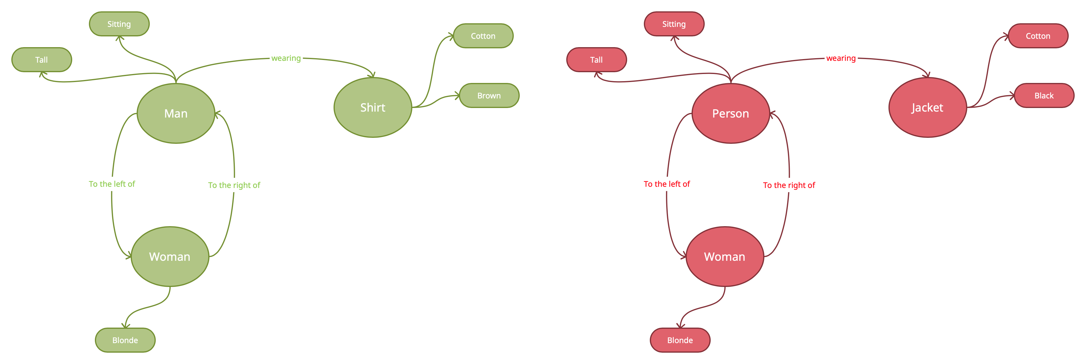
Figure 2: (Left) Ground truth scene graph and (Right) Generated noisy scene graph

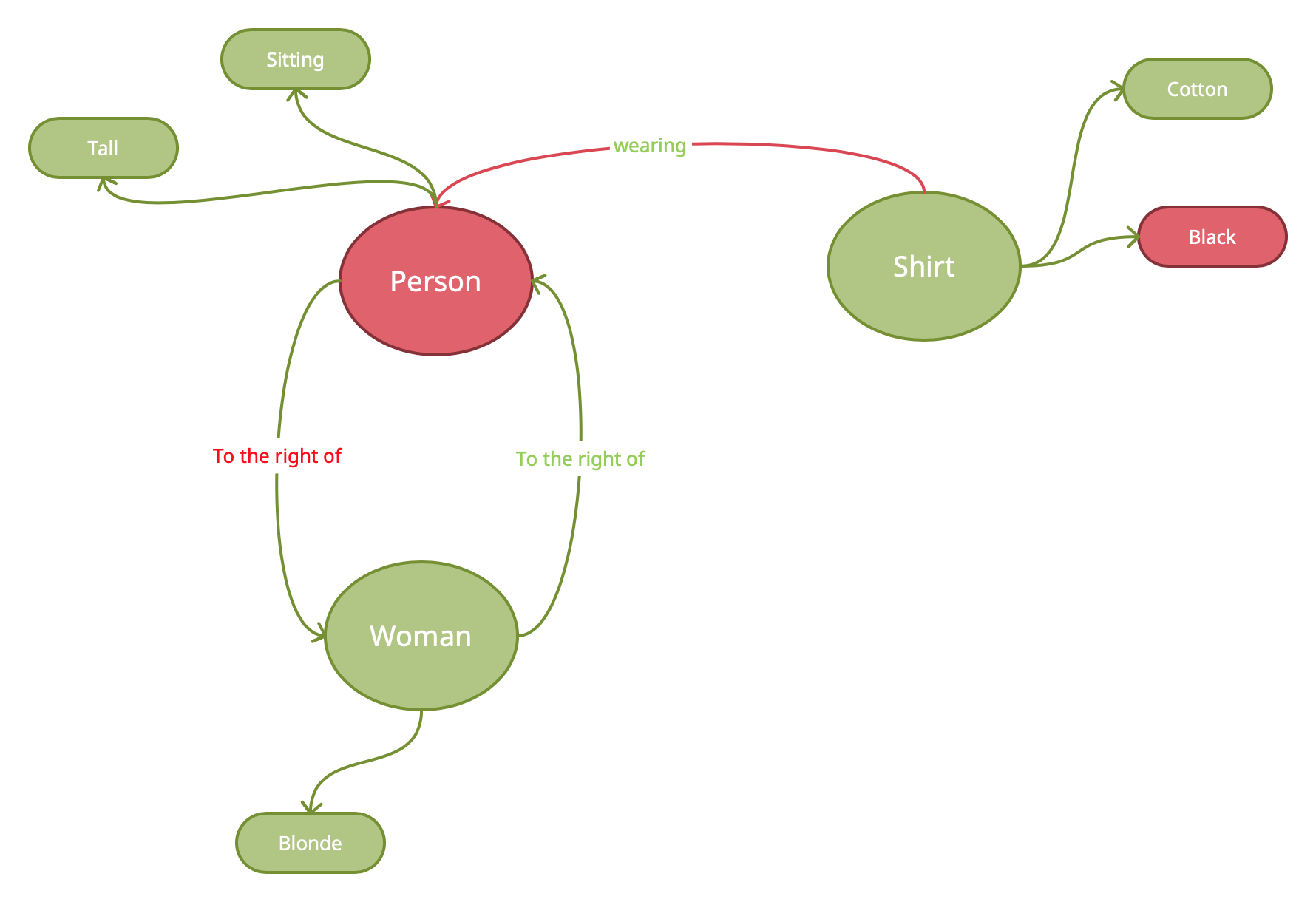
(a) Scene graph generated after injecting noise

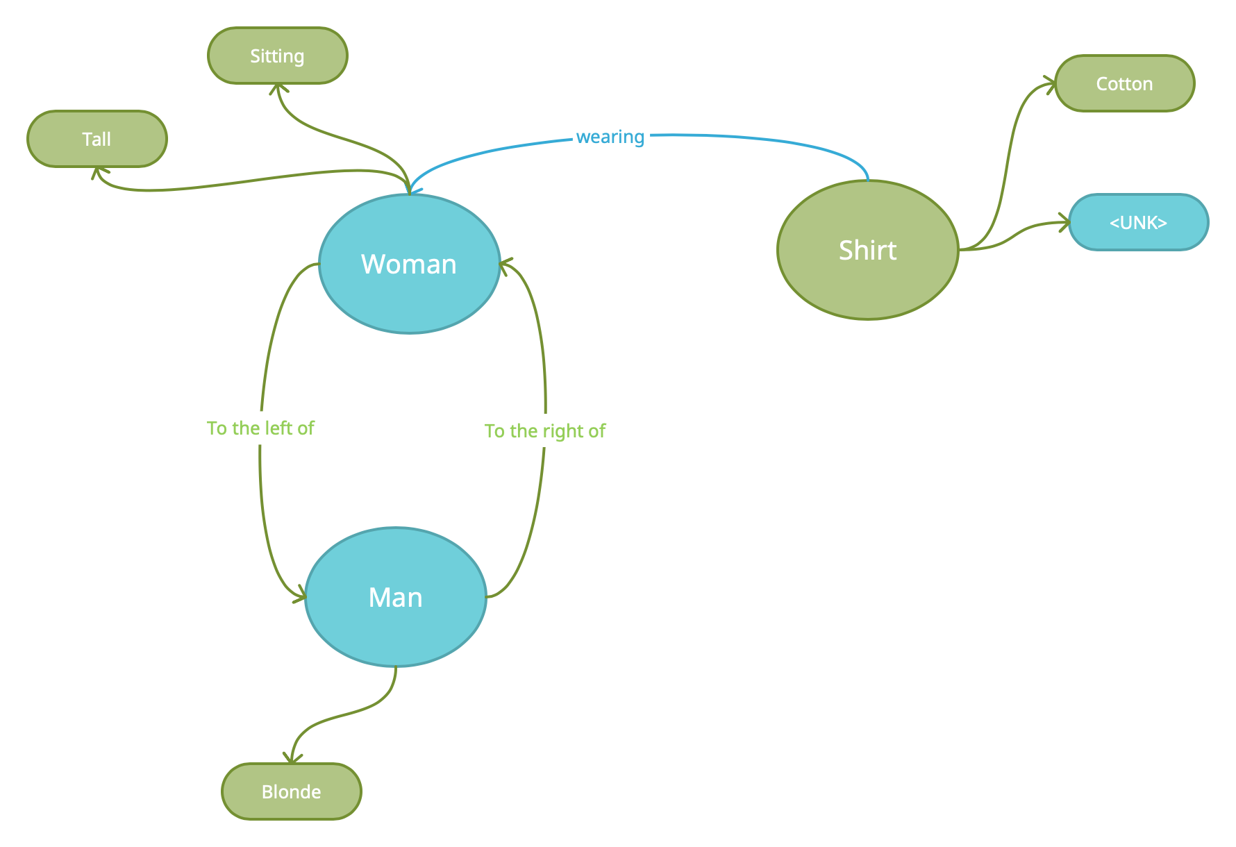
(b) Scene graph generated after corrupting ground truth

Figure 3: Noisy/Corrupted Scene graph representations

Since test images are evaluated on the noisy scene graphs, we propose a novel training curriculum to ensure the Graph Network representation is able to capture maximum information from the generated scene graphs. A Graph Network trained on only ground truth scene graphs encodes scene graphs for test images poorly since there is a large difference in the representations of ground truth and generated scene graphs due to differences in quality.

In order to train a model to have strong low-level features, we first train the Graph Network on ground truth scene graphs for 2 epochs and slowly introduce features of the noisy scene graphs into the ground truth scene graphs by randomly swapping out nodes, edge pairs and relations between the two (ground truth and noisy) graphs. The degree with which noise is introduced is controlled by 2 parameters: the probability with which noise is introduced into the scene graph and the proportion of the components for which we switch out with noisy counterparts. For example, if probability is 0.5 and proportion is 0.8 and we have 10 edges, then there is a 50% chance that we switch out 8 ground truth edges with noisy edges. This injection of noise is slowly introduced while training the model with an increasing probability and proportion (of components) with each passing epoch.

Maintaining a steady probabilistic approach of injecting noise into the ground truth scene graphs allows the model to have superior lower-level feature extraction as well as high-level semantic extraction in the upper layer more akin to the noisy graph features. Figures 2 and 3(a) illustrate how a swap happens between components of the two scene graphs. We also experiment with switching out the entire graph (replace ground truth with noisy) at random during training, and with models that are trained on a mixed dataset.

4.7 UNITER with Scene Graphs

Given the success of pre-trained models across a wide range of tasks, we seek to use scene graphs with uniter. While the task-specific nature of mac allowed us to replace the image with the scene graph, doing so with uniter would not work since only image representations were fed to the model during pre-training. Hence, we adopt the late fusion architecture shown in Figure 4, where the output of an sgmac model trained on ground truth scene graphs is passed through fully-connected layers and the output of a pre-trained uniter model is passed through separate fully-connected layers. The outputs of these layers are then combined and passed through a classification layer. The fully-connected layers are trained from scratch, while sgmac and uniter are fine-tuned.

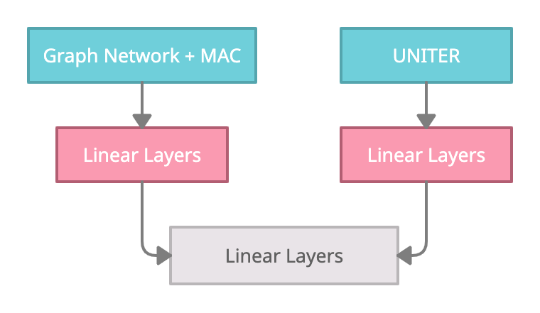
Figure 4: uniter with Scene Graphs

5 Experimental Setup

Throughout the course of this project, we primarily work with the GQA dataset, where we analyze the effects of using scene graphs instead of images to aid our models in the task of VQA.

5.1 Dataset

The GQA dataset consists of 22M+ questions and 113K+ images, with associated scene graphs for 85K+ images. The dataset is divided into 5 splits: train, validation, testdev, test and challenge, with the option to avail a more balanced subset for most categories. The test and challenge datasets are used for leaderboard submissions and do not come with ground truth scene graphs. The training and validation sets are provided with images which have annotated ground truth scene graphs. Apart from the ground truth scene graphs which we leverage for our experiments, we also use the extracted object features and spatial features, provided with the dataset, in our baseline models.

The GQA task uses six metrics to evaluate a model’s visual reasoning ability, namely accuracy, validity, plausibility, consistency, grounding, and distribution. Details about the calculation of each metric can be found in the GQA paper (Hudson and Manning, 2019b).

5.2 Training Environment

The experimental setup for this project can be divided into various components based on how the training phase is carried out. The details regarding the various training stages and requirements are outlined in Table 1.

Training phase	Scene Graph Generation	GQA Answering Model
Model Architecture	ResNet 50 + Neural Motifs	GN + mac	uniter
Optimizer	SGD	Adam	AdamW
Learning rate	0.02	1e-4	8e-5
Epochs / Steps	50000 steps	15 epochs	6000 steps
Batch size	4	128	500
No. of GPUs	4	1	2
GPU Model / RAM	Tesla V100 / 32 GB	Tesla V100 / 16 GB	Tesla V100 / 16 GB
Time taken	1 day 18 hours	22.5 hours	45 minutes

Table 1: Experimental settings of various models and stages of training

6 Results and Analysis

In this section, we present the results of our proposed approach along with an extensive analysis. We use the semantic types in A.1 for our analysis.

6.1 Results of Baselines

Our Models		Comparable Models
Model	Test	Model	Test
Image	0.174	CNN	0.178
Text	0.398	LSTM	0.41
concat	0.435	CNN+LSTM	0.465
attn	0.48	Bottom-up	0.497

Table 2: Comparison of Baselines

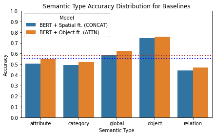
Figure 5: Comparison of the two baselines

Model	Val	Testdev
uniter	0.69	0.598
sgmac (GT)	0.94	-
sgmac (Noisy)	0.548	0.478
sgmac + uniter	0.688	0.592

Table 3: Results of Proposed Approaches

From Table 2 we see that the text only baseline does much better than the image only one. This is expected, as the question has more useful information to infer the answer than the image alone. The attn model achieves a significantly higher accuracy than concat. We believe that the attention mechanism helps attn focus on the most relevant objects in the image, based on the question at hand.

Figure 5 shows the breakdown of the performance of both baselines on questions of different semantic types. attn does better than concat in every category. We see that there is a large scope for improvement in all the semantic types, especially in the relation type which primarily consists of questions that require knowledge about the relationships between objects to answer. This information can be found in the scene graphs.

6.2 Performance of UNITER

Figure 6 shows the performance of uniter over the different semantic types. The performance across all the types far exceeds that of the baselines, demonstrating the strength of uniter’s image-text representations and the advantages of pre-training. It is interesting to note that the relative ordering of semantic type accuracy is the same for uniter and the baselines. The accuracy on the object type is very high, while there is large room for improvement in the relation type. An analysis of the predictions of the model shows that for many examples, the model predicts an answer that is semantically close to the ground truth answer (e.g. ’bananas’ vs ’banana’, ’desk’ vs ’table’). Here, it is useful to look to metrics other than accuracy which do not enforce an exact match with the ground truth answer. uniter obtains high plausibility (0.92) and validity (0.95) scores, indicating a good understanding of the image and text.

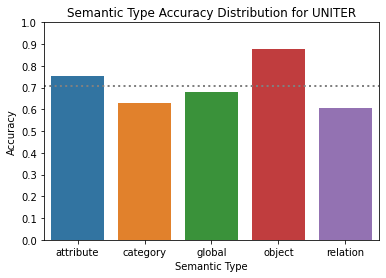
Figure 6: Performance of uniter over semantic types

6.3 SGMAC on GT Scene Graphs

The performance of sgmac with GT scene graphs on different semantic types is shown in Figure 7. This approach does very well over all types, and most notably the relation semantic type where uniter struggles. The overall validation accuracy of this approach is 94.6%. This shows the effectiveness of the scene graph representation, and perhaps represents the upper limit of what can be achieved on GQA .

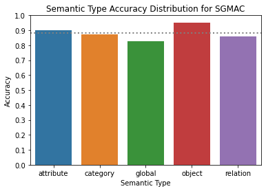
Figure 7: Performance of sgmac on ground truth scene graphs

6.3.1 SGMAC vs SGATT

The attention model described in Section 4.1 with the Graph Network (66.4% accuracy) does not match the performance of sgmac with the Graph Network (94.5% accuracy), even when trained and evaluated on ground truth scene graphs. This demonstrates the importance of the manner in which the scene graph is parsed and proves that a good scene graph representation alone is not sufficient to achieve high accuracy.

6.4 GT vs Generated Scene Graphs

Figure 8 shows a comparison of the semantic type accuracy of sgmac with GT scene graphs and noisy scene graphs. It is clear that the performance of sgmac with ground truth scene graphs far exceeds that of sgmac with noisy scene graphs on attribute, category and relation types and has a comparable performance on global and object types. We believe that this is due to the quality of the generated scene graphs rather than the technique used to encode them.

Scene Graphs	Val
GT	0.945
GT - No Relations	0.851
GT - No Attributes	0.851
Noisy	0.529
Noisy - No Relations	0.532
Noisy - No Attributes	0.53

Table 4: sgmac performance on different scene graphs

To get a better idea of the differences between the generated and ground truth scene graphs, we analyze their corresponding objects, attributes and relations.

Objects: On average, GT scene graphs have 16 objects, and 3 of these are not present in the generated scene graphs. Since most objects are correctly detected, the model correctly answers the majority of questions about the existence of objects in the image (object semantic type). The performance on this type using GT and generated scene graphs is comparable due to the high overlap in the objects.

Attributes: We find that most attributes in the GT scene graphs are present in the generated scene graphs. However, the generated scene graphs additionally contain many spurious attributes, which negates the effect of getting the attributes right and explains the poor performance on the attribute semantic type. For example, a phone which is grey in color might also have “blue” and “brown” as additional attributes, and hence a question such as “What color is the phone?” would not be answered correctly. In Sec. 6.5.3 we describe the use of thresholds to reduce spurious attributes.

Relations: We find that most of the edges have extremely low overlap (1-2 edges) between GT and noisy scene graphs, which explains why the gap between the performance of the two on the relation semantic type is high.

The above analysis showcases the need for improvement in the quality of the generated scene graphs. Specifically, correctly detecting relations would go a long way towards improving performance. It also shows how the use of accurate scene graphs would benefit VQA.

In addition to qualitative analysis, we conduct the ablation studies shown in Table 4 to understand the impact of various components of scene graphs. We run experiments wherein we remove either relation names or attributes from the scene graph. On removing relations/attributes from GT scene graphs, we observe a 9.4% drop in accuracy. The same experiments when run on generated scene graphs yield little difference in accuracy further indicating that the quality of detected relations is poor.

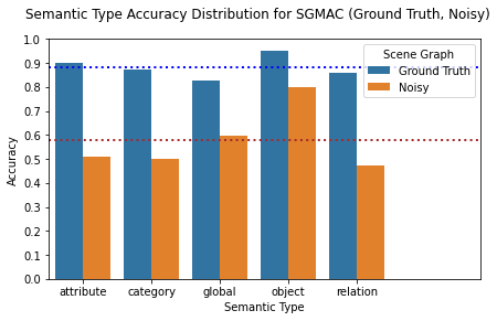
Figure 8: Comparison of sgmac using ground truth and noisy scene graphs

6.5 Effect of scene graph quality

We further experiment with various scene graphs outputs that were generated by different variations of the Neural Motifs model, to effectively analyze the difference in quality of the scene graphs generated. We experiment with 2 variations of the model, making changes to the loss function to better understand the differences in prediction pertaining to the predicted labels for an edge relation. The variations are as follows:

6.5.1 Impact of Label Loss Smoothing

During a preliminary analysis of the dataset, we noticed that there is a stark imbalance in the training data for the relation labels “to the left of” and “to the right of”. Both labels appear at least 18 times more often than next most frequent relation in the training set. This causes the standard variant of our model to disproportionately predict the above mentioned relations. In an attempt to mitigate this class imbalance, we use an exponential label smoothing loss function.

Model	Testdev
Without Smoothing - Noisy	0.458
Without Smoothing - GT + Noisy	0.479
With Smoothing - Noisy	0.457
With Smoothing - GT + Noisy	0.476

Table 5: sgmac performance with and without label smoothing

We can see from Table 5 that the label smoothing does not help improve the downstream model performance much. Another potential remedy to handle the class imbalance would be to use a two-way softmax that separates the “to the left of ” and “to the right of” labels from the other relations.

6.5.2 Corruption of GT Scene Graphs

Level of Corruption	Val
0.2	0.861
0.4	0.788
0.6	0.721
0.8	0.662
Noisy	0.461

Table 6: sgmac performance with different levels of scene graph corruption

In order to understand how the noisy scene graphs affect downstream performance in our GQA model, we conduct evaluation of our best performing GT (sgmac) model on varying levels of corrupted ground truth scene graphs. This allows us to estimate the amount of noise it would take in a gold standard scene graph dataset to reach the same accuracy we obtain when evaluated on a noisy scene graph dataset. In order to corrupt the ground truth scene graphs, we randomly swap nodes, edge pairs and relations, and also corrupt object attributes and names by replacing them with UNK tokens. Figure 3(b) illustrates an example of what a corrupted ground truth scene graph would look like, in contrast to the ground truth scene graph, as depicted on the left side of Figure 2. These differ from the noisy injected scene graphs (Section 4.6) as we do not bring in any external components from the noisy scene graphs into the corrupted GT scene graph. We create 4 validation datasets of different levels of corruption by varying degrees of probability with which we corrupt the scene graph as shown in Table 6. From the table it is clear that the noisy scene graphs differ much more significantly from the ground truth representations and that this level of noisiness will be very hard to overcome even with the most powerful model capable of reasoning over scene graphs.

6.5.3 Filtering Predicted Scene Graphs

In order to remove any redundant or spurious information that is included while generating the noisy scene graphs, we also employ some standard filtering techniques to take the top k components of the noisy scene graph. In an unfiltered noisy scene graph, we would have 80 objects, 10 attributes/object and 100 relations between object pairs. From this set, we employ two filtering strategies based on both the confidence score of the model for each label and also based on the top k labels the model predicts.

For the top k setting, we take the top 40 objects, the top 3 attributes/object and the top 80 relations from each noisy scene graph. We also alternatively filter them by a threshold value and only include components that are greater than a particular threshold. The threshold values selected are 0.1 for objects, 0.9 for attributes and 0.8 for relations.

Scene Graph Filter	Testdev
No Filter - Noisy	0.468
Top k - Noisy	0.464
Threshold - Noisy	0.458
No Filter - GT + Noisy	0.475
Top k - GT + Noisy	0.478
Threshold - GT + Noisy	0.479

Table 7: sgmac performance with different filters on scene graphs

When training from scratch, retaining all the model attributes and relations intact seems to let the model learn more information with further training. This indicates that the filtered noisy scene graphs are possibly more akin to the ground truth representations but without a good lower level feature representation (a good starting checkpoint), the Graph Network might not be powerful enough to learn much from the (sparsely) filtered noisy scene graphs.

6.6 Training Curriculum

Training Curriculum	Testdev
GT	0.373
Noisy	0.468
GT+Noisy	0.475
Probabilistic	0.471
Probabilistic (Filtered)	0.477
Probabilistic (Complete)	0.478

Table 8: Training Curriculum Results

As mentioned in Section 4.6, we see that training with just the GT and or just noisy scene graphs does not yield very desirable results. However, training the model using the novel training curriculum outlined in Section 4.6 gives us a gain in performance.

We see that gradually swapping ground truth scene graphs with noisy scene graphs during training (Probabilistic (Complete) in 8) performs better than completely replacing ground truth scene graphs with noisy scene graphs after a few epochs (GT + Noisy in 8). Completely replacing the ground truth scene graphs (for random noisy graphs) performs on par with the probabilistic training mechanism explained in Figure 2 and 3(a).

We see that filtering the noisy dataset on the top k objects/attributes/relations helps weed out the redundant/spurious labels and improve accuracy slightly. Overall, these results prove that the probabilistic training curriculum helps the model generalize much better compared to training on one source of data, and hence validate the effectiveness of the proposed novel training curriculum.

6.7 UNITER with Scene Graphs

The late-fusion ensemble of uniter with sgmac does not perform better than uniter itself. We analyse the accuracies across semantic types to see if it does better on relational queries, but find no significant differences. It could be that uniter is a very powerful model which overwhelms the much smaller sgmac.

7 Conclusion and Future Work

In this work, we present novel research that is aimed at understanding various aspects of the use of scene graphs for the task of VQA. We develop modules for scene graph encoding, architectures for question answering using scene graphs, probabilistic training curricula, and late fusion models for question answering. We primarily use validation and test-dev scores for our analysis, but our test submissions can be found on the leaderboard under the team name “bert”.

The architecture combining a Graph Network with mac surpasses the performance of state of the art models when ground truth scene graphs are available. However, this performance quickly deteriorates as reliance on auto-generated scene graphs increases. We show that a training curriculum that utilizes generated and ground truth scene graphs is more effective than the use of a singular type of scene graph. This approach does not come close to matching pre-trained image based models such as uniter, suggesting that improving scene graph generation will be the most important step for using scene graph based models for VQA. Tackling the class imbalance for relations and improving the object detection could help in this regard. Techniques that allow the model to fall-back to image features based on the level of noise in the scene graph could be quite effective and we plan to explore these further.

Appendix A Appendices

A.1 Semantic Types in GQA

GQA classifies its questions into 5 semantic types:

1. Relation: subject/object of a described relation, e.g. “What furniture is the beer can on?”

2. Attribute: properties/position of an object, e.g. “What is the color of the man’s shirt?”

3. Object: existence of objects in the image, e.g. “Are there any wine glasses or cups?”

4. Category: object identification within a class, e.g. “Which kind of clothing is maroon?”

5. Global: overall scene properties, e.g. “How’s the weather?”

References

- Agrawal et al. (2018) Aishwarya Agrawal, Dhruv Batra, Devi Parikh, and Aniruddha Kembhavi. 2018. Don’t just assume; look and answer: Overcoming priors for visual question answering. In Proceedings of the IEEE Conference on Computer Vision and Pattern Recognition, pages 4971–4980.
- Anderson et al. (2018) Peter Anderson, Xiaodong He, Chris Buehler, Damien Teney, Mark Johnson, Stephen Gould, and Lei Zhang. 2018. Bottom-up and top-down attention for image captioning and visual question answering. In Proceedings of the IEEE conference on computer vision and pattern recognition, pages 6077–6086.
- Andreas et al. (2016) Jacob Andreas, Marcus Rohrbach, Trevor Darrell, and Dan Klein. 2016. Neural module networks. In Proceedings of the IEEE conference on computer vision and pattern recognition, pages 39–48.
- Antol et al. (2015) Stanislaw Antol, Aishwarya Agrawal, Jiasen Lu, Margaret Mitchell, Dhruv Batra, C Lawrence Zitnick, and Devi Parikh. 2015. Vqa: Visual question answering. In Proceedings of the IEEE international conference on computer vision, pages 2425–2433.
- Battaglia et al. (2018) Peter W Battaglia, Jessica B Hamrick, Victor Bapst, Alvaro Sanchez-Gonzalez, Vinicius Zambaldi, Mateusz Malinowski, Andrea Tacchetti, David Raposo, Adam Santoro, Ryan Faulkner, et al. 2018. Relational inductive biases, deep learning, and graph networks. arXiv preprint arXiv:1806.01261.
- Chen et al. (2020) Yen-Chun Chen, Linjie Li, Licheng Yu, Ahmed El Kholy, Faisal Ahmed, Zhe Gan, Yu Cheng, and Jingjing Liu. 2020. Uniter: Universal image-text representation learning. In European Conference on Computer Vision, pages 104–120. Springer.
- Devlin et al. (2019) Jacob Devlin, Ming-Wei Chang, Kenton Lee, and Kristina Toutanova. 2019. BERT: Pre-training of deep bidirectional transformers for language understanding. In Proceedings of the 2019 Conference of the North American Chapter of the Association for Computational Linguistics: Human Language Technologies, Volume 1 (Long and Short Papers), pages 4171–4186, Minneapolis, Minnesota. Association for Computational Linguistics.
- He et al. (2017) Kaiming He, Georgia Gkioxari, Piotr Dollár, and Ross Girshick. 2017. Mask r-cnn. In Proceedings of the IEEE international conference on computer vision, pages 2961–2969.
- Hudson and Manning (2019a) Drew Hudson and Christopher D Manning. 2019a. Learning by abstraction: The neural state machine. In Advances in Neural Information Processing Systems, pages 5903–5916.
- Hudson and Manning (2018) Drew A Hudson and Christopher D Manning. 2018. Compositional attention networks for machine reasoning. arXiv preprint arXiv:1803.03067.
- Hudson and Manning (2019b) Drew A Hudson and Christopher D Manning. 2019b. Gqa: A new dataset for real-world visual reasoning and compositional question answering. In Proceedings of the IEEE Conference on Computer Vision and Pattern Recognition, pages 6700–6709.
- Johnson et al. (2018) Justin Johnson, Agrim Gupta, and Li Fei-Fei. 2018. Image generation from scene graphs.
- Johnson et al. (2017) Justin Johnson, Bharath Hariharan, Laurens van der Maaten, Li Fei-Fei, C Lawrence Zitnick, and Ross Girshick. 2017. Clevr: A diagnostic dataset for compositional language and elementary visual reasoning. In Proceedings of the IEEE Conference on Computer Vision and Pattern Recognition, pages 2901–2910.
- Krishna et al. (2017) Ranjay Krishna, Yuke Zhu, Oliver Groth, Justin Johnson, Kenji Hata, Joshua Kravitz, Stephanie Chen, Yannis Kalantidis, Li-Jia Li, David A Shamma, et al. 2017. Visual genome: Connecting language and vision using crowdsourced dense image annotations. International journal of computer vision, 123(1):32–73.
- Lee et al. (2020) Hsin-Ying Lee, Lu Jiang, Irfan Essa, Phuong B Le, Haifeng Gong, Ming-Hsuan Yang, and Weilong Yang. 2020. Neural design network: Graphic layout generation with constraints.
- Lee et al. (2019) S. Lee, J. Kim, Y. Oh, and J. H. Jeon. 2019. Visual question answering over scene graph. In 2019 First International Conference on Graph Computing (GC), pages 45–50.
- Li et al. (2019) Yijun Li, Lu Jiang, and Ming-Hsuan Yang. 2019. Controllable and progressive image extrapolation.
- Liang et al. (2019) J. Liang, L. Jiang, L. Cao, Y. Kalantidis, L. Li, and A. G. Hauptmann. 2019. Focal visual-text attention for memex question answering. IEEE Transactions on Pattern Analysis and Machine Intelligence, 41(8):1893–1908.
- Pennington et al. (2014) Jeffrey Pennington, Richard Socher, and Christopher Manning. 2014. GloVe: Global vectors for word representation. In Proceedings of the 2014 Conference on Empirical Methods in Natural Language Processing (EMNLP), pages 1532–1543, Doha, Qatar. Association for Computational Linguistics.
- Ren et al. (2016) Shaoqing Ren, Kaiming He, Ross Girshick, and Jian Sun. 2016. Faster r-cnn: Towards real-time object detection with region proposal networks. IEEE transactions on pattern analysis and machine intelligence, 39(6):1137–1149.
- Tan and Bansal (2019) Hao Tan and Mohit Bansal. 2019. Lxmert: Learning cross-modality encoder representations from transformers. arXiv preprint arXiv:1908.07490.
- Tang et al. (2020) Kaihua Tang, Yulei Niu, Jianqiang Huang, Jiaxin Shi, and Hanwang Zhang. 2020. Unbiased scene graph generation from biased training. In Proceedings of the IEEE/CVF Conference on Computer Vision and Pattern Recognition, pages 3716–3725.
- Tang et al. (2019) Kaihua Tang, Hanwang Zhang, Baoyuan Wu, Wenhan Luo, and Wei Liu. 2019. Learning to compose dynamic tree structures for visual contexts. In Proceedings of the IEEE Conference on Computer Vision and Pattern Recognition, pages 6619–6628.
- Xu et al. (2017) Danfei Xu, Yuke Zhu, Christopher B Choy, and Li Fei-Fei. 2017. Scene graph generation by iterative message passing. In Proceedings of the IEEE conference on computer vision and pattern recognition, pages 5410–5419.
- Zellers et al. (2018) Rowan Zellers, Mark Yatskar, Sam Thomson, and Yejin Choi. 2018. Neural motifs: Scene graph parsing with global context. In Proceedings of the IEEE Conference on Computer Vision and Pattern Recognition, pages 5831–5840.
- Zhou et al. (2018) Jie Zhou, Ganqu Cui, Zhengyan Zhang, Cheng Yang, Zhiyuan Liu, Lifeng Wang, Changcheng Li, and Maosong Sun. 2018. Graph neural networks: A review of methods and applications. arXiv preprint arXiv:1812.08434.