Towards Practical Adam: Non-Convexity, Convergence Theory, and Mini-Batch Acceleration

Abstract

Adam is one of the most influential adaptive stochastic algorithms for training deep neural networks, which has been pointed out to be divergent even in the simple convex setting via a few simple counterexamples. Many attempts, such as decreasing an adaptive learning rate, adopting a big batch size, incorporating a temporal decorrelation technique, seeking an analogous surrogate, etc., have been tried to promote Adam-type algorithms to converge. In contrast with existing approaches, we introduce an alternative easy-to-check sufficient condition, which merely depends on the parameters of the base learning rate and combinations of historical second-order moments, to guarantee the global convergence of generic Adam for solving large-scale non-convex stochastic optimization. This observation, coupled with this sufficient condition, gives much deeper interpretations on the divergence of Adam. On the other hand, in practice, mini-Adam and distributed-Adam are widely used without any theoretical guarantee. We further give an analysis on how the batch size or the number of nodes in the distributed system affects the convergence of Adam, which theoretically shows that mini-batch and distributed Adam can be linearly accelerated by using a larger mini-batch size or a larger number of nodes. At last, we apply the generic Adam and mini-batch Adam with the sufficient condition for solving the counterexample and training several neural networks on various real-world datasets. Experimental results are exactly in accord with our theoretical analysis.

Keywords: Adam, non-convexity, convergence rate, mini-batch/distributed Adam, linear speedup.

1 Introduction

Large-scale non-convex stochastic optimization (Bottou et al., 2018), covering a slew of applications in statistics and machine learning (Jain et al., 2017; Bottou et al., 2018) such as learning a latent variable from massive data whose probability density distribution is unknown, takes the following generic formulation:

$$\min_{\bm{x}\in\mathbb{R}^{d}}\ f(\bm{x})=\mathbb{E}_{\xi\sim\mathbb{P}}\,\big{[}\widetilde{f}(\bm{x},\xi)\big{]},$$ (1)

where $f(\bm{x})$ is a non-convex function and $\xi$ is a random variable with an unknown distribution $\mathbb{P}$.

Alternatively, a compromised approach to handle this difficulty is to use an unbiased stochastic estimate of $\bm{\nabla}\!{f}(\bm{x})$, denoted as $g(\bm{x},\xi)$, which leads to the stochastic gradient descent (SGD) algorithm (Robbins and Monro, 1985). Its coordinate-wise version is defined as follows:

$$\bm{x}_{t+1,k}=\bm{x}_{t,k}-\eta_{t,k}\bm{g}_{t,k}(\bm{x}_{t},\xi_{t}),$$ (2)

for $k=1,2,\ldots,d$, where $\eta_{t,k}\geq 0$ is the learning rate of the $k$-th component of stochastic gradient $\bm{g}(\bm{x}_{t},\xi_{t})$ at the $t$-th iteration. Under some mild assumptions (e.g., the optimal solution exists), a sufficient condition (Robbins and Monro, 1985) to ensure the global convergence of vanilla SGD in Eq. (2) is to require $\eta_{t}$ to meet the following diminishing condition:

$$\sum_{t=1}^{\infty}\|\eta_{t}\|=\infty\ {\rm\ and\ }\ \sum\limits_{t=1}^{\infty}\|\eta_{t}\|^{2}<\infty.$$ (3)

Although the vanilla SGD algorithm with learning rate $\eta_{t}$ satisfying condition (3) does converge, its empirical performance could be still stagnating, since it is difficult to tune an effective learning rate $\eta_{t}$ via condition (3).

To further improve the empirical performance of SGD, a large variety of adaptive SGD algorithms, including AdaGrad (Duchi et al., 2011), RMSProp (Hinton et al., 2012), Adam (Kingma and Ba, 2014), Nadam (Dozat, 2016), AdaBound (Luo et al., 2019), etc., have been proposed to automatically tune the learning rate $\eta_{t}$ by using second-order moments of historical stochastic gradients $\{\bm{g}_{t}\}$. Let $\bm{v}_{t,k}$ and $\bm{m}_{t,k}$ be the exponential moving average of the historical second-order moments $(\bm{g}^{2}_{1,k},\bm{g}^{2}_{2,k},\cdots,\bm{g}^{2}_{t,k})$ and stochastic gradient estimates $(\bm{g}_{1,k},\bm{g}_{2,k},\cdots,\bm{g}_{t,k})$, respectively. More specifically, two groups of hyperparameters ($\beta_{t}$, $\theta_{t}$) will be involved into the calculation of $m_{t,k}=\beta_{t}m_{t-1,k}+(1-\beta_{t})g_{t,k}$ and $v_{t,k}=\theta_{t}v_{t-1,k}+(1-\theta_{t})g^{2}_{t,k}$. Then, the generic iteration scheme of these adaptive SGD algorithms (Reddi et al., 2018; Chen et al., 2018a) is summarized as

$$\!\!\bm{x}_{t+1,k}\!=\bm{x}_{t,k}-\eta_{t,k}\bm{m}_{t,k},\ {\rm\ with\ }\eta_{t,k}\!={\alpha_{t}}/{\sqrt{\bm{v}_{t,k}}},\!\!$$ (4)

for $k=1,2,\ldots,d$, where $\alpha_{t}>0$ is called base learning rate and it is independent of stochastic gradient estimates $(\bm{g}_{1,k},\bm{g}_{2,k},\cdots,\bm{g}_{t,k})$ for all $t\geq 1$. Although Adam works well for solving large scale convex and non-convex optimization problems such as training deep neural networks, it has been disclosed to be divergent in some scenarios via counterexamples (Reddi et al., 2018). Thus, without any further assumptions for corrections, Adam should not be directly used. Recently, developing sufficient conditions to guarantee global convergences of Adam -type algorithms has attracted much attention from both machine learning and optimization communities. The existing successful attempts can be divided into four categories: decreasing a learning rate, adopting a big batch size, incorporating a temporal decorrelation, and seeking an analogous surrogate. However, some of them are either hard to check or impractical. In this work, we will first introduce an alternative easy-to-check sufficient condition to guarantee the global convergences of the original Adam.

Meanwhile, in practice, stochastic Adam, where a single sample is used to estimate gradient, converges slowly to the optimal point. People usually use mini-batch Adam instead to get faster convergence performance. In SGD, although how the sample size will affect the convergence has been well studied (Li et al., 2014), few works give analysis on mini-batch adaptive gradient methods especially on Adam, since mini-batch size largely affects adaptive learning rate $\eta_{t,k}$ in Eq .(4), which makes the analysis difficult. In this work, we give the first complexity analysis for mini-batch Adam, which shows that mini-batch Adam can also be theoretically accelerated by using a larger mini-batch size.

On the other hand, as the data size goes larger in machine learning problems, it is hard to collect, store and process data in a single machine. Several machines are involved in the optimization process. Hence, distributed optimization methods are proposed, where distributed Adam is also popularly used. Different from mini-batch Adam, where only one machine is used for optimization, several machines are involved. In the distributed setting, machines are connected via a network graph. More specifically, there are two kinds of structures used in distributed Adam: parameter-server structure and decentralized structure. In the parameter-server structure, there is one special machine called as parameter server and the rest called workers. The parameter server connects to all workers, but workers don’t connect to each other. Therefore, workers can share information with the parameter server in each communication round but cannot share information with the other workers. However, in the decentralized structure, there is not a server involved in the structure. A pre-defined graph connects all machines. A machine can only share information with its direct neighbors in each communication round. Still, few works answer how the local batch size and number of machines will affect the convergence of distributed Adam. In this work, because the analysis of distributed Adam under the parameter-server model is similar to Mini-batch Adam, we answer this question and show that distributed Adam under a parameter-server model can also achieve a linear speedup property as distributed SGD (Yu et al., 2019).

In summary, the contributions of this work are five-fold:

• We introduce an easy-to-check sufficient condition to ensure the global convergences (i.e., averaged expected gradient norm converges to 0) of generic Adam in the common smooth non-convex stochastic setting with mild assumptions. Moreover, this sufficient condition is distinctive from the existing conditions and is easier to verify.

• We provide a new explanation on the divergences of original Adam and RMSProp, which are possibly due to an incorrect parameter setting of the combinations of historical second-order moments.

• We find that the sufficient condition extends the restrictions of RMSProp (Mukkamala and Hein, 2017) and covers many convergent variants of Adam, e.g., AdamNC, AdaGrad with momentum, etc. Thus, their convergences in the non-convex stochastic setting naturally hold.

• We theoretically show that mini-batch Adam can be further accelerated by adopting a larger mini-batch size, and that distributed Adam can achieve a linear speed up property in the parameter-server distributed system by using commonly used sufficient condition parameters.

• We conduct experiments to validate the sufficient condition for the convergences of Adam and mini-batch Adam. The experimental results match our theoretical results.

The paper is organized as follows. In Section 2, we first give the formulation of generic Adam and then discuss several works related to Adam including several existing sufficient convergence conditions, analysis of mini-batch, and distributed stochastic gradient methods. In Section 3, we derive the sufficient condition for convergence of Adam and provide several insights for the divergence of vanilla Adam. In Section 4, we give the complexity analysis on practical Adam with a commonly used sufficient condition parameter, including mini-batch Adam and distributed Adam. At last, in Section 5, we conduct some experiments under both theoretical settings and practical settings to verify the established theory. In addition, by practical Adam, we mean that we give a thorough analysis for Adam, mini-batch Adam, and distributed Adam, which have been commonly used for training deep neural networks without theoretical guarantees.

2 Related work

2.1 Generic Adam

For readers’ convenience, we first clarify a few necessary notations used in the forthcoming Generic Adam. First, we denote $\bm{x}_{t,k}$ as the $k$-th component of $\bm{x}_{t}\in\mathbb{R}^{d}$, and $\bm{g}_{t,k}$ as the $k$-th component of the stochastic gradient at the $t$-th iteration respectively, and call $\alpha_{t}>0$ base learning rate and $\beta_{t}$ momentum parameter, respectively. Let $\epsilon>0$ be a sufficiently small constant. Denote $\bm{0}=(0,\cdots,0)^{\top}\in\mathbb{R}^{d}$, and $\bm{\epsilon}=(\epsilon,\cdots,\epsilon)^{\top}\in\mathbb{R}^{d}$. All operations, such as multiplying, dividing, and taking the square root, are executed in the coordinate-wise mode.

Algorithm 1  Generic Adam

1:  Parameters: Set suitable base learning rate $\{\alpha_{t}\}$, momentum parameter $\{\beta_{t}\}$, and exponential moving average parameter $\{\theta_{t}\}$, respectively. Choose $\bm{x}_{1}\in\mathbb{R}^{d}$ and set initial values $\bm{m}_{0}=\bm{0}\in\mathbb{R}^{d}$ and $\bm{v}_{0}=\bm{\epsilon}\in\mathbb{R}^{d}$.

2:  for $t=1,\,2,\,\ldots,\,T$ do

3:     Sample a stochastic gradient $\bm{g}_{t}$;

4:     for $k=1,\,2,\,\ldots,\,d$ do

5:        $\bm{v}_{t,k}=\theta_{t}\bm{v}_{t-1,k}+(1-\theta_{t})\bm{g}_{t,k}^{2}$;

6:        $\bm{m}_{t,k}=\beta_{t}\bm{m}_{t-1,k}+(1-\beta_{t})\bm{g}_{t,k}$;

7:        $\bm{x}_{t+1,k}=\bm{x}_{t,k}-{\alpha_{t}\bm{m}_{t,k}}/\sqrt{\bm{v}_{t,k}}$;

8:     end for

9:  end for

It is not hard to check that Generic Adam covers RMSProp by setting $\beta_{t}=0$ directly. Moreover, it covers Adam with a bias correction (Kingma and Ba, 2014) as follows:

Remark 1.

The vanilla Adam with the bias correction (Kingma and Ba, 2014) takes constant parameters $\beta_{t}=\beta$ and $\theta_{t}=\theta$. The iteration scheme is written as $\bm{x}_{t+1}=\bm{x}_{t}-\widehat{\alpha}_{t}\frac{\widehat{\bm{m}}_{t}}{\sqrt{\widehat{\bm{v}}_{t}}}$, with $\widehat{\bm{m}}_{t}=\frac{\bm{m}_{t}}{1-\beta^{t}}$ and $\widehat{\bm{v}}_{t}=\frac{\bm{v}_{t}}{1-\theta^{t}}$. Let $\alpha_{t}=\widehat{\alpha}_{t}\frac{\sqrt{1-\theta^{t}}}{1-\beta^{t}}$. Then, the above can be rewritten as $\bm{x}_{t+1}=\bm{x}_{t}-{\alpha_{t}\bm{m}_{t}}/\sqrt{\bm{v}_{t}}$. Thus, it is equivalent to taking constant $\beta_{t}$, constant $\theta_{t}$, and new base learning rate $\alpha_{t}$ in Generic Adam.

2.2 Convergence Conditions for Adam

First, because Reddi et al. (2018) gave counterexamples on divergence of origin Adam, several sufficient conditions have been proposed to guarantee global convergences of Adam that can be summarized into the following four categories:

(C1) Decreasing a learning rate.   Reddi et al. (2018) have declared that the core cause of divergences of Adam and RMSProp is largely controlled by the difference between the two adjacent learning rates, i.e.,

$$\Gamma_{t}={1}/{\bm{\eta}_{t}}-{1}/{\bm{\eta}_{t-1}}={\sqrt{\bm{v}_{t}}}/{\alpha_{t}}-{\sqrt{\bm{v}_{t-1}}}/{\alpha_{t-1}}.$$ (5)

Once positive definiteness of $\Gamma_{t}$ is violated, Adam and RMSProp may suffer from divergence (Reddi et al., 2018). Based on this observation, two variants of Adam called AMSGrad and AdamNC have been proposed with convergence guarantees in both the convex (Reddi et al., 2018) and non-convex (Chen et al., 2018a) stochastic settings by requiring $\Gamma_{t}\succ 0$. In addition, Padam (Zhou et al., 2018a) extended from AMSGrad has been proposed to contract the generalization gap in training deep neural networks, whose convergence has been ensured by requiring $\Gamma_{t}\succ 0$. As a relaxation of $\Gamma_{t}\succ 0$, Barakat and Bianchi (2020) showed that when $\alpha_{t}/\sqrt{v_{t}}\leq\alpha_{t-1}/(c\sqrt{v_{t-1}})$ holds for all $t$ and some positive $c$, the algorithm Adam can converge. In the strongly convex stochastic setting, by using the long-term memory technique developed in (Reddi et al., 2018), Huang et al. (2018) have proposed NosAdam by attaching more weights on historical second-order moments to ensure its convergence. Prior to that, the convergence rate of RMSProp (Mukkamala and Hein, 2017) has already been established in the convex stochastic setting by employing similar parameters to those of AdamNC (Reddi et al., 2018).

(C2) Adopting a big batch size.   Basu et al. (2018), for the first time, showed that deterministic Adam and RMSProp with original iteration schemes are convergent by using a full-batch gradient. On the other hand, both Adam and RMSProp can be reshaped as specific signSGD-type algorithms (Balles and Hennig, 2018; Bernstein et al., 2018) whose $\mathcal{O}(1/\sqrt{T})$ convergence rates have been provided in the non-convex stochastic setting by setting batch size as large as the number of maximum iterations (Bernstein et al., 2018). Recently, Zaheer et al. (2018) have established $\mathcal{O}(1/\sqrt{T})$ convergence rate of original Adam directly in the non-convex stochastic setting by requiring the batch size to be the same order as the number of maximum iterations. We comment that this type of requirement is impractical when Adam and RMSProp are applied to tackle large-scale problems (1), since these approaches cost a huge number of computations to estimate big-batch stochastic gradients in each iteration.

(C3) Incorporating a temporal decorrelation.   By exploring the structure of the convex counterexample in (Reddi et al., 2018), Zhou et al. (2018b) have pointed out that the divergence of RMSProp is fundamentally caused by the imbalanced learning rate rather than the absence of $\Gamma_{t}\succ 0$. Based on this viewpoint, Zhou et al. (2018b) have proposed AdaShift by incorporating a temporal decorrelation technique to eliminate the inappropriate correlation between $\bm{v}_{t,k}$ and the current second-order moment $\bm{g}_{t,k}^{2}$, in which the adaptive learning rate $\eta_{t,k}$ is required to be independent of $\bm{g}^{2}_{t,k}$. However, the convergence of AdaShift in (Zhou et al., 2018b) was merely restricted to RMSProp for solving the convex counterexample in (Reddi et al., 2018).

(C4) Seeking an analogous surrogate.  Due to the divergences of Adam and RMSProp (Reddi et al., 2018), Zou et al. (2018) proposed a class of new surrogates called AdaUSM to approximate Adam and RMSProp by integrating weighted AdaGrad with a unified heavy ball and Nesterov accelerated gradient momentums. Its $\mathcal{O}(\log{(T)}/\sqrt{T})$ convergence rate has also been provided in the non-convex stochastic setting by requiring a non-decreasing weighted sequence. Besides, many other adaptive stochastic algorithms without combining momentums, such as AdaGrad (Ward et al., 2018; Li and Orabona, 2019) and stagewise AdaGrad (Chen et al., 2018b), have been guaranteed to be convergent and work well in the non-convex stochastic setting.

In contrast with the above four types of modifications and restrictions, we introduce an alternative easy-to-check sufficient condition (abbreviated as (SC)) to guarantee the global convergences of original Adam. The proposed (SC) merely depends on the parameters in estimating $\bm{v}_{t,k}$ and base learning rate $\alpha_{t}$. (SC) neither requires the positive definiteness of $\Gamma_{t}$ like (C1) nor needs the batch size as large as the same order as the number of maximum iterations like (C2) in both the convex and non-convex stochastic settings. Thus, it is easier to verify and more practical compared with (C1)-(C3). On the other hand, (SC) is partially overlapped with (C1) since the proposed (SC) can cover AdamNC (Reddi et al., 2018), AdaGrad with exponential moving average (AdaEMA) momentum (Chen et al., 2018a), and RMSProp (Mukkamala and Hein, 2017) as instances whose convergences are all originally motivated by requiring the positive definiteness of $\Gamma_{t}$. While, based on (SC), we can directly derive their global convergences in the non-convex stochastic setting as byproducts without checking the positive definiteness of $\Gamma_{t}$ step by step. Besides, (SC) can serve as an alternative explanation on divergences of original Adam and RMSProp, which are possibly due to incorrect parameter settings for accumulating the historical second-order moments rather than the imbalanced learning rate caused by the inappropriate correlation between $\bm{v}_{t,k}$ and $\bm{g}^{2}_{t,k}$ like (C3). In addition, AdamNC and AdaEMA are convergent under (SC), but violate (C3) in each iteration. Meanwhile, there are lots of work improving upper bounds for the above algorithms, e.g., Défossez et al. (2020) improved the constants related to $\beta$ by introducing a novel average scheme in the analysis.

2.3 Mini-batch Stochastic Gradient Methods

In practice, people usually use mini-batch stochastic gradient methods instead of single sample stochastic gradient methods or full gradient methods for faster convergence. For mini-batch SGD algorithms, Li et al. (2014) have shown that mini-batch SGD boosts $\mathcal{O}(\frac{1}{\sqrt[4]{T}})$ convergence rate of SGD to $\mathcal{O}(\frac{1}{\sqrt[4]{sT}})$ where $s$ is the mini-batch size. However, as it is much harder to show the convergence of adaptive gradient methods, few works analyze how sample size will affect the convergence of the adaptive gradient algorithms. Li and Orabona (2019) gave an analysis on Adagrad and showed the convergence rate is linear in the sample size. Zaheer et al. (2018) gave the analysis on Adam, showing that large batch size can help convergence, but the batch size should increase with iteration increasing, which may not be practical. In this work, we theoretically show that mini-batch Adam can be accelerated by adopting a larger mini-batch size as mini-batch SGD (Li et al., 2014) in the same order.

2.4 Distributed Stochastic Gradient Methods

Distributed stochastic gradient descent was first introduced in Agarwal and Duchi (2011) in the parameter-server setting. Further, in the decentralized setting, Lian et al. (2017) gave the analysis on the stochastic gradient descent. The analysis shows that the convergence speed will be linear in the number of workers in the parameter-server setting or will be linear to some constant related to the decentralized graph structure. For the adaptive gradient methods, in the parameter-server setting, Reddi et al. (2020) gave algorithms in the federated scenario called FedAdam, FedAdagrad, and FedYogi. Moreover, they showed that the convergence speed will be linear in the number of workers. However, instead divided by $\sqrt{\bm{v}_{t}}$, they divide the gradient with $\sqrt{\bm{v_{t}}+\bm{\epsilon}}$. Meanwhile, in their assumptions, $\epsilon$ in the algorithm should be in the order of $O(\frac{G}{L})$, where $G$ is the upper bound of gradient norm, and $L$ is the Lipschitz constant of the objective function. However, in practice, $\epsilon$ is always set to be a small value, much smaller than $G/L$. On the other hand, the large $\epsilon$ may dominate the adaptive term in their algorithms. Hence, their methods may degrade to stochastic gradient descent. Carnevale et al. (2020) shoed that Adam with gradient tracking method can be linearly accelerated with an increasing number of nodes in the decentralized and strongly convex setting. Still, it is unclear whether, in the nonconvex setting, this linear speedup will hold when Adam is used. Moreover, Chen et al. (2020) gave an analysis of Adagrad and showed the convergence speed will be linear in the number of workers. Meanwhile, Nazari et al. (2019) gave the analysis of Adagrad in the decentralized setting. Xie et al. (2019) also gave a variant on Adagrad algorithm called AdaAlter in the centralized setting and showed the convergence will linearly speed up by increasing the number of workers. Recently, Chen et al. (2021, 2022) extend Adam to the distributed quantized Adam with error compensation technique Stich et al. (2018). However, the linear speedup property in (Chen et al., 2021, 2022) does not hold. To the best of our knowledge, whether the distributed Adam can achieve a linear speedup is still open. This paper theoretically demonstrates that the distributed Adam in the parameter-server model can achieve a linear speedup concerning the number of workers.

3 Novel Sufficient Condition for Convergence of Adam

In this section, we characterize the upper-bound of gradient residual of problem (1) as a function of parameters $(\theta_{t},\alpha_{t})$. Then the convergence rate of Generic Adam is derived directly by specifying appropriate parameters $(\theta_{t},\alpha_{t})$. Below, we state the necessary assumptions that are commonly used for analyzing the convergence of a stochastic algorithm for non-convex problems:

(A1)

The minimum value of problem (1) is lower-bounded, i.e., $f^{*}=\min_{\bm{x}\in\mathbb{R}^{d}}\ f(\bm{x})>-\infty$;

(A2)

The gradient of $f$ is $L$-Lipschitz continuous, i.e., $\|\bm{\nabla}\!f(\bm{x})-\bm{\nabla}\!f(\bm{y})\|\!\leq\!L\|\bm{x}\!-\!\bm{y}\|,\ \forall\bm{x},\bm{y}\!\in\!\mathbb{R}^{d}$;

(A3)

The stochastic gradient $\bm{g}_{t}$ is an unbiased estimate, i.e., $\mathbb{E}\,[\bm{g}_{t}]=\bm{\nabla}\!{f}_{t}(\bm{x}_{t})$;

(A4)

The second-order moment of stochastic gradient $\bm{g}_{t}$ is uniformly upper-bounded, i.e., $\mathbb{E}\,\|\bm{g}_{t}\|^{2}\leq G$.

In addition, we also suppose that the parameters $\{\beta_{t}\}$, $\{\theta_{t}\}$, and $\{\alpha_{t}\}$ satisfy the following restrictions:

(R1)

The parameters $\{\beta_{t}\}$ satisfy $0\leq\beta_{t}\leq\beta<1$ for all $t$ for some constant $\beta$;

(R2)

The parameters $\{\theta_{t}\}$ satisfy $0<\theta_{t}<1$ and $\theta_{t}$ is non-decreasing in $t$ with $\theta:=\lim\limits_{t\to\infty}\theta_{t}>\beta^{2}$;

(R3)

The parameters $\{\alpha_{t}\}$ satisfy that $\chi_{t}:=\frac{\alpha_{t}}{\sqrt{1-\theta_{t}}}$ is “almost” non-increasing in $t$, by which we mean that there exist a non-increasing sequence $\{a_{t}\}$ and a positive constant $C_{0}$ independent of $t$ such that $a_{t}\leq\chi_{t}\leq C_{0}a_{t}$.

The restriction (R3) indeed says that $\chi_{t}$ is the product between some non-increasing sequence $\{a_{t}\}$ and some bounded sequence. This is a slight generalization of $\chi_{t}$ itself being non-decreasing. If $\chi_{t}$ itself is non-increasing, we can then take $a_{t}=\chi_{t}$ and $C_{0}=1$. For most of the well-known Adam-type methods, $\chi_{t}$ is indeed non-decreasing. For instance, for AdaGrad with EMA momentum we have $\alpha_{t}=\eta/\sqrt{t}$ and $\theta_{t}=1-1/t$, so $\chi_{t}=\eta$ is constant; for Adam with constant $\theta_{t}=\theta$ and non-increasing $\alpha_{t}$ (say $\alpha_{t}=\eta/\sqrt{t}$ or $\alpha_{t}=\eta$), $\chi_{t}=\alpha_{t}/\sqrt{1-\theta}$ is non-increasing. The motivation, instead of $\chi_{t}$ being decreasing, is that it allows us to deal with the bias correction steps in Adam (Kingma and Ba, 2014).

We fix a positive constant $\theta^{\prime}>0$ such that $\beta^{2}<\theta^{\prime}<\theta$. Let $\gamma:={\beta^{2}}/{\theta^{\prime}}<1$ and

$$C_{1}:=\prod_{j=1}^{N}\big{(}\frac{\theta_{j}}{\theta^{\prime}}\big{)},$$ (6)

where $N$ is the maximum of the indices $j$ with $\theta_{j}<\theta^{\prime}$. The finiteness of $N$ is guaranteed by the fact that $\lim_{t\to\infty}\theta_{t}=\theta>\theta^{\prime}$. When there are no such indices, i.e., $\theta_{1}\geq\theta^{\prime}$, we take $C_{1}=1$ by convention. In general, $C_{1}\leq 1$. Our main results on estimating gradient residual state as follows:

Theorem 2.

Let $\{\bm{x}_{t}\}$ be a sequence generated by Generic Adam for initial values $\bm{x}_{1}$, $\bm{m}_{0}=\bm{0}$, and $\bm{v}_{0}=\bm{\epsilon}$. Assume that $f$ and stochastic gradients $\bm{g}_{t}$ satisfy assumptions (A1)-(A4). Let $\tau$ be randomly chosen from $\{1,2,\ldots,T\}$ with equal probabilities $p_{\tau}=1/T$. Then, we have

$$\mathbb{E}\left[\left\|\bm{\nabla}f(\bm{x}_{\tau})\right\|\right]\leq\sqrt{\frac{C+C^{\prime}\sum_{t=1}^{T}\alpha_{t}\sqrt{1-\theta_{t}}}{T\alpha_{T}}},$$

where $C^{\prime}\!=\!{2C_{0}^{2}C_{3}d\sqrt{G^{2}\!+\!\epsilon d}}{\big{/}}{[(1\!-\!\beta)\theta_{1}]}$ and

$$\begin{split}C=\frac{2C_{0}\sqrt{G^{2}\!+\!\epsilon d}}{1-\beta}\big{[}(C_{4}\!+\!C_{3}C_{0}d\chi_{1}\log\big{(}1\!+\!\frac{G^{2}}{\epsilon d}\big{)}\big{]},\end{split}$$

in which $C_{4}$ and $C_{3}$ are defined as $C_{4}=f(x_{1})-f^{*}$ and $C_{3}=\frac{C_{0}}{\sqrt{C_{1}}(1-\sqrt{\gamma})}\big{[}\frac{C_{0}^{2}\chi_{1}L}{C_{1}(1-\sqrt{\gamma})^{2}}+2\big{(}\frac{\beta/(1-\beta)}{\sqrt{C_{1}(1-\gamma)\theta_{1}}}+1\big{)}^{2}G\big{]}$, respectively.

Remark 3.

Below, we give two comments on the above Theorem:
(i) The constants $C$ and $C^{\prime}$ depend on priory known constants $C_{0},C_{1},\beta,\theta^{\prime},G,L,\epsilon,d,f^{*},\theta_{1},\alpha_{1},\bm{x}_{1}$.
(ii) Convergence in expectation in the above theorem is on the term $\mathbb{E}[\left\|\nabla f(\bm{x}_{\tau})\right\|]$ which is slightly weaker than $\mathbb{E}[\left\|\nabla\!f(\bm{x}_{\tau})\right\|^{2}]$. The latter form holds for most SGD variants with global learning rates, namely, the learning rate for each coordinate is the same, because $\frac{1}{\sum_{t=1}^{T}\!\alpha_{t}}\mathbb{E}\sum_{t=1}^{T}\!\alpha_{t}\left\|\nabla\!f(\bm{x}_{t})\right\|^{2}$ is exactly $\mathbb{E}[\left\|\nabla\!f(\bm{x}_{\tau})\right\|^{2}]$ if $\tau$ is randomly selected via distribution $\mathbb{P}(\tau\!=\!k)\!=\!\frac{\alpha_{k}}{\sum_{t=1}^{T}\!\alpha_{t}}$. This does not apply to coordinate-wise adaptive stochastic methods because the learning rate for each coordinate is different, and hence unable to randomly select an index according to some distribution uniform for each coordinate. On the other hand, the convergence rates of AMSGrad and AdaEMA (Chen et al., 2018a) are able to achieve the bound for $\mathbb{E}[\left\|\nabla\!f(\bm{x}_{\tau})\right\|^{2}]$. This is due to the strong assumption $\left\|g_{t}\right\|\leq G$ which results in a uniform lower bound for each coordinate of the adaptive learning rate $\eta_{t,k}\!\geq\!\alpha_{t}/G$. Thus, the proof of AMSGrad (Chen et al., 2018a) can be dealt with in a way similar to the case of global learning rate. In our paper we use a coordinate-wise adaptive learning rate and assume a weaker assumption $\mathbb{E}[\left\|g_{t}\right\|^{2}]\!\leq\!G$ instead of $\left\|g_{t}\right\|^{2}\!\leq\!G$.

3.1 Proof Sketch of Theorem 2

In this section, we will give some important lemmas that will be used to prove Theorem 2. First, for simplicity, we give some notations used in the lemmas and proof. Denote $\hat{\bm{v}}_{t}=\theta_{t}\bm{v}_{t-1}+(1-\theta_{t})\mathbb{E}\left[\bm{g}_{t}^{2}|\bm{x}_{t}\right]$, $\hat{\bm{\eta}}_{t}=\alpha_{t}/\sqrt{\hat{\bm{v}}_{t}}$, $\bm{\Delta}_{t}=\alpha_{t}\bm{m}_{t}/\sqrt{\bm{v}_{t}}$, and $\left\|\bm{x}\right\|^{2}_{\bm{\hat{\eta}}}=\sum_{i=1}^{d}\bm{\hat{\eta}}_{i}\bm{x}_{i}^{2}$.

Lemma 4.

Let $\{\bm{x}_{t}\}$ be the sequence generated by Algorithm 1. For $T\geq 1$, it holds that

$$f^{*}\leq f(\bm{x}_{1})+\sum_{t=1}^{T}\mathbb{E}\left[\left\langle\bm{\nabla}f(\bm{x}_{t}),\bm{\Delta}_{t}\right\rangle+L\left\|\bm{\Delta}_{t}\right\|^{2}\right].$$

Lemma 4 is widely used to prove convergence of the stochastic gradient algorithms. To further prove the convergence related to gradient norm, we introduce the following lemma to bound term $\sum_{t=1}^{T}\mathbb{E}\left[\left\langle\bm{\nabla}f(\bm{x}_{t}),\bm{\Delta}_{t}\right\rangle+L\left\|\bm{\Delta}_{t}\right\|^{2}\right]$.

Lemma 5.

(Lemma 33 in Appendix) Let $\{\bm{x}_{t}\}$ be the sequence generated by Algorithm 1. For $T\geq 1$, it holds that

$$\begin{split}\sum_{t=1}^{T}\mathbb{E}\left[\left\langle\bm{\nabla}f(\bm{x}_{t}),\bm{\Delta}_{t}\right\rangle+L\left\|\bm{\Delta}_{t}\right\|^{2}\right]\leq-\frac{1-\beta}{2}\mathbb{E}\left[\sum_{t=1}^{T}\left\|\bm{\nabla}f(\bm{x}_{t})\right\|_{\bm{\hat{\eta}}_{t}}^{2}\right]+\frac{\zeta_{0}}{\theta_{1}}\sum_{t=1}^{T}\alpha_{t}\sqrt{1-\theta_{t}}+\zeta_{1},\end{split}$$

for some constants $\zeta_{0}$ and $\zeta_{1}$.

With Lemma 5, we obtain the upper bound for $\mathbb{E}\left[\sum_{t=1}^{T}\left\|\bm{\nabla}f(\bm{x}_{t})\right\|_{\bm{\hat{\eta}}_{t}}^{2}\right]$ with respect to $\alpha_{t},\ \theta_{t},$ and $\beta$. To prove Lemma 5, the most important step is to remove dependence between the adaptive learning rate and stochastic gradient. Hence, $\hat{\eta}_{t}$ is introduced, as it is independent of the stochastic gradient. The rest of the proof is just bounding the error of introducing $\hat{\bm{\eta}}_{t}$ instead of using $\alpha_{t}/\sqrt{\bm{v}_{t}}$. Then, the last step is to build connection between $\frac{1}{T}\mathbb{E}[\left\|\bm{\nabla}f(\bm{x}_{t})\right\|]$ and $\mathbb{E}\left[\sum_{t=1}^{T}\left\|\bm{\nabla}f(\bm{x}_{t})\right\|_{\bm{\eta}_{t}}^{2}\right]$.

Lemma 6.

(Lemma 36 in Appendix) Let $\tau$ be an integer that is randomly chosen from $\{1,2,\cdots,T\}$ with equal probabilities. We have the following estimate

$$\mathbb{E}[\left\|\bm{\nabla}f(\bm{x}_{\tau})\right\|]\leq\sqrt{\frac{\zeta_{2}}{T\alpha_{T}}\mathbb{E}\left[\sum_{t=1}^{T}\left\|\bm{\nabla}f(\bm{x}_{t})\right\|^{2}_{\hat{\bm{\eta}}_{t}}\right]},$$

for some constant $\zeta_{2}$.

Thus, using the above three lemmas, we can prove Theorem 2.

3.2 Discussion of Theorem 2

Corollary 7.

Take $\alpha_{t}=\eta/t^{s}$ with $0\leq s<1$. Suppose $\lim_{t\to\infty}\theta_{t}=\theta<1$. Define $Bound(T):=\frac{C+C^{\prime}\sum_{t=1}^{T}\alpha_{t}\sqrt{1-\theta_{t}}}{T\alpha_{T}}$. Then the $Bound(T)$ in Theorem 2 is bounded from below by constants

$$Bound(T)\geq C^{\prime}\sqrt{1-\theta}.$$ (7)

In particular, when $\theta_{t}=\theta<1$, we have the following more subtle estimate of lower and upper-bounds for $Bound(T)$

$$\frac{C}{\eta T^{1-s}}+C^{\prime}\sqrt{1-\theta}\leq Bound(T)\!\leq\!\frac{C}{\eta T^{1-s}}\!+\!\frac{C^{\prime}\sqrt{1\!-\!\theta}}{1-s}.$$

Remark 8.

(i) Corollary 7 shows that if $\lim_{t\to\infty}\theta_{t}=\theta<1$, the bound in Theorem 2 is only $\mathcal{O}(1)$, hence not guaranteeing convergence. This result is not surprising as Adam with constant $\theta_{t}$ has already shown to be divergent (Reddi et al., 2018). Hence, $\mathcal{O}(1)$ is its best convergence rate we can expect. We will discuss this case in more details in Section 3.4.
(ii) Corollary 7 also indicates that in order to guarantee convergence, the parameter has to satisfy $\lim_{t\to\infty}\theta_{t}=1$. Although we do not assume this in our restrictions (R1)-(R3), it turns out to be the consequence from our analysis. Note that if $\beta<1$ in (R1) and $\lim_{t\to\infty}\theta_{t}=1$, then the restriction $\lim_{t\to\infty}\theta_{t}>\beta^{2}$ is automatically satisfied in (R2).

We are now ready to give the Sufficient Condition for convergence of Generic Adam.

Corollary 9 (Sufficient Condition(SC)).

Generic Adam is convergent if the parameters $\{\alpha_{t}\}$, $\{\beta_{t}\}$, and $\{\theta_{t}\}$ satisfy the following four conditions:

• $0\leq\beta_{t}\leq\beta<1$;

• $0<\theta_{t}<1$ and $\theta_{t}$ is non-decreasing in $t$;

• $\chi_{t}:=\alpha_{t}/\sqrt{1-\theta_{t}}$ is “almost” non-increasing;

• $\big{(}{\sum_{t=1}^{T}\alpha_{t}\sqrt{1-\theta_{t}}}\big{)}{\big{/}}\big{(}{T\alpha_{T}}\big{)}=o(1)$.

3.3 Convergence Rate of Generic Adam

We now provide the convergence rate of Generic Adam with specific parameters $\{(\theta_{t},\alpha_{t})\}$, i.e.,

$$\alpha_{t}=\eta/t^{s}\text{~{}~{}and~{}~{}}\theta_{t}=\left\{\begin{aligned} &1-\alpha/K^{r},\quad&t<K,\\ &1-\alpha/t^{r},\quad&t\geq K,\end{aligned}\right.$$ (8)

for positive constants $\alpha,\eta,K$, where $K$ is taken such that $\alpha/K^{r}<1$. Note that $\alpha$ can be taken bigger than 1. When $\alpha<1$, we can take $K=1$ and then $\theta_{t}=1-\alpha/t^{r},t\geq 1$. To guarantee (R3), we require $r\leq 2s$. For such a family of parameters we have the following corollary.

Corollary 10.

Generic Adam with the above family of parameters (i.e. (8)) converges as long as $0<r\leq 2s<2$, and its non-asymptotic convergence rate is given by

$$\mathbb{E}[\left\|\bm{\nabla}f(\bm{x}_{\tau})\right\|]\leq\left\{\begin{aligned} &\mathcal{O}(T^{-r/4}),\quad&r/2+s<1\\ &\mathcal{O}(\sqrt{\log(T)/T^{1-s}}),\quad&r/2+s=1\\ &\mathcal{O}(1/T^{(1-s)/2}),\quad&r/2+s>1\end{aligned}\right..$$

Remark 11.

Corollary 10 recovers and extends the results of some well-known algorithms below:

• AdaGrad with exponential moving average (EMA). When $\theta_{t}=1-1/t$, $\alpha_{t}=\eta/\sqrt{t}$, and $\beta_{t}=\beta<1$, Generic Adam is exactly AdaGrad with EMA momentum (AdaEMA) (Chen et al., 2018a). In particular, if $\beta=0$, this is the vanilla coordinate-wise AdaGrad. It corresponds to taking $r=1$ and $s=1/2$ in Corollary 10. Hence, AdaEMA has convergence rate $\mathcal{O}\left(\sqrt{\log(T)/\sqrt{T}}\right)$.

• AdamNC. Taking $\theta_{t}=1-1/t$, $\alpha_{t}=\eta/\sqrt{t}$, and $\beta_{t}=\beta\lambda^{t}$ in Generic Adam, where $\lambda<1$ is the decay factor for the momentum factors $\beta_{t}$, we recover AdamNC (Reddi et al., 2018). Its $\mathcal{O}\left(\sqrt{\log{(T)}/\sqrt{T}}\right)$ convergence rate can be directly derived via Corollary 10.

• RMSProp. Mukkamala and Hein (2017) have reached the same $\mathcal{O}\left(\sqrt{\log{(T)}/\sqrt{T}}\right)$ convergence rate for RMSprop with $\theta_{t}=1-\alpha/t$, when $0<\alpha\leq 1$ and $\alpha_{t}=\eta/\sqrt{t}$ under the convex assumption. Since RMSProp is essentially Generic Adam with all momentum factors $\beta_{t}=0$, we recover Mukkamala and Hein’s results by taking $r=1$ and $s=1/2$ in Corollary 10. Moreover, our result generalizes to the non-convex stochastic setting, and it holds for all $\alpha\!>\!0$ rather than only $0\!<\!\alpha\!\leq\!1$.

The summarization of the above algorithms is provided in Table 1.

Algorithm	$\theta_{t}$	$\alpha_{t}$	$\beta_{t}$	Convergence Result
Adagrad with EMA (Chen et al. (2018a))	$1-1/t$	$\eta/\sqrt{t}$	$\beta$	$\mathcal{O}(\sqrt{\log T/\sqrt{T}})$
AdamNC (Reddi et al. (2018))	$1-1/t$	$\eta/\sqrt{t}$	$\beta\lambda^{t}$	$\mathcal{O}(\sqrt{\log T/\sqrt{T}})$
RMSProp (Mukkamala and Hein, 2017)	$1-\alpha/t$	$\eta/\sqrt{t}$	0	$\mathcal{O}(\sqrt{\log T/\sqrt{T}})$

Table 1: Convergence results for some well-known algorithms

Comparison with Reddi et al. (2018) .  Most of the convergent modifications of original Adam, such as AMSGrad, AdamNC, and NosAdam, all require $\Gamma_{t}\succ 0$ in Eq. (5), which is equivalent to decreasing the adaptive learning rate $\eta_{t}$ step by step. Since the term $\Gamma_{t}$ (or adaptive learning rate $\eta_{t}$) involves the past stochastic gradients (hence not deterministic), the modification to guarantee $\Gamma_{t}\succ 0$ either needs to change the iteration scheme of Adam (like AMSGrad) or needs to impose some strong restrictions on the base learning rates $\alpha_{t}$ and $\theta_{t}$ (like AdamNC). Our sufficient condition provides an easy-to-check criterion for the convergence of Generic Adam in Corollary 9. It is not necessary to require $\Gamma_{t}\succ 0$. Moreover, we use exactly the same iteration scheme as the original Adam without any modifications. Our work shows that the positive definiteness of $\Gamma_{t}$ may not be an essential issue for the divergence of the original Adam. The divergence may be due to the incorrect setting of moving average parameters instead of non-positive definiteness of $\Gamma_{t}$.

3.4 Constant $\theta_{t}$ case: insights for divergence

The currently most popular RMSProp and Adam’s parameter setting takes constant $\theta_{t}$, i.e., $\theta_{t}=\theta<1$. The motivation behind is to use the exponential moving average of squares of past stochastic gradients. In practice, parameter $\theta$ is recommended to be set very close to 1. For instance, a commonly adopted $\theta$ is taken as 0.999.

Although great performance in practice has been observed, such a constant parameter setting has the serious flaw that there is no convergence guarantee even for convex optimization, as proved by the counterexamples in (Reddi et al., 2018). Ever since much work has been done to analyze the divergence issue of Adam and to propose modifications with convergence guarantees, as summarized in the introduction section. However, there is still not a satisfactory explanation that touches the fundamental reason for the divergence. In this section, we try to provide more insights for the divergence issue of Adam/RMSProp with constant parameter $\theta_{t}$, based on our analysis of the sufficient condition for convergence.

From the sufficient condition perspective.   Let $\alpha_{t}\!=\!\eta/t^{s}$ for $0\leq s\!<\!1$ and $\theta_{t}\!=\!\theta\!<\!1$. According to Corollary 7, $Bound(T)$ in Theorem 2 has the following estimate:

$$\frac{C}{\eta T^{1\!-s}}\!+\!C^{\prime}\sqrt{1\!-\!\theta}\!\leq\!Bound(T)\!\leq\!\frac{C}{\eta T^{1-s}}\!+\!\frac{C^{\prime}\sqrt{1\!-\!\theta}}{(1\!-s)}.$$

The bounds tell us some points on Adam with constant $\theta_{t}$:

• $Bound(T)\!=\!\mathcal{O}(1)$, so the convergence is not guaranteed. This result coincides with the divergence issue demonstrated in (Reddi et al., 2018). Indeed, since in this case Adam is not convergent, this is the best bound we can have.

• Consider the dependence on parameter $s$. The bound is decreasing in $s$. The best bound in this case is when $s=0$, i.e., the base learning rate is taken constant. This explains why in practice taking a more aggressive constant base learning rate often leads to even better performance, comparing with taking a decaying one.

• Consider the dependence on parameter $\theta$. Note that the constants $C$ and $C^{\prime}$ depend on $\theta_{1}$ instead of the whole sequence $\theta_{t}$. We can always set $\theta_{t}=\theta$ for $t\geq 2$ while fix $\theta_{1}<\theta$, by which we can take $C$ and $C^{\prime}$ independent of constant $\theta$. Then the principal term of $Bound(T)$ is linear in $\sqrt{1-\theta}$, so decreases to zero as $\theta\to 1$. This explains why setting $\theta$ close to 1 often results in better performance in practice.

Moreover, Corollary 10 shows us how the convergence rate continuously changes when we continuously vary parameters $\theta_{t}$. Let us fix $\alpha_{t}\!=\!1/\sqrt{t}$ and consider the following continuous family of parameters $\{\theta_{t}^{(r)}\}$ with $r\in[0,1]$:

$$\theta_{t}^{(r)}=1-\alpha^{(r)}/t^{r},\text{~{}~{}where~{}~{}}\alpha^{(r)}=r\bar{\theta}+(1-\bar{\theta}),\ 0<\bar{\theta}<1.$$

Note that when $r=1$, then $\theta_{t}=1-1/t$, this is the AdaEMA, which has the convergence rate $\mathcal{O}\left(\sqrt{\log T/\sqrt{T}}\right)$; when $r=0$, then $\theta_{t}=\bar{\theta}<1$, this is the original Adam with constant $\theta_{t}$, which only has the $\mathcal{O}(1)$ bound; when $0<r<1$, by Corollary 10, the algorithm has the $\mathcal{O}(T^{-r/4})$ convergence rate. Along with this continuous family of parameters, we observe that the theoretical convergence rate continuously deteriorates as the real parameter $r$ decreases from 1 to 0, namely, as we gradually shift from AdaEMA to Adam with constant $\theta_{t}$. In the limiting case, the latter is not guaranteed with convergence anymore.

4 Complexity Analysis for Practical Adam: Mini-batch/Distributed Adam

Due to the limited time, limited computational resources, and noise in data collection and processing, it is almost impossible to achieve the accurate stationary point. Thus, instead of achieving the accurate stationary point, people get more attention to achieving some approximated stationary point in practice. The crucial question under this situation will become how much time is needed to achieve some approximated solution. This section will answer this question by answering how many iterations are needed to obtain an $\varepsilon$-stationary point. First, we define $\varepsilon$-stationary point as follows:

Definition 12.

We define a random variable $\bm{x}$ as an $\varepsilon$-stationary point of problem (1), if

$$\mathbb{E}_{\bm{x}}\left[\left\|\mathbb{E}_{\xi\sim\mathbb{P}}\left[\nabla\tilde{f}(\bm{x},\xi)\right]\right\|\right]\leq\varepsilon.$$

According to Definition 12 and Theorem 2, for generic Adam, we can directly give the following corollary:

Corollary 13.

For any $\varepsilon>0$, if we take $T\geq C_{5}^{2}\varepsilon^{-4}$, $\alpha_{t}=\frac{\alpha}{\sqrt{T}},\ \beta_{t}=\beta,\theta_{t}=1-\frac{\theta}{T}$, which satisfy $\gamma=\frac{\beta}{1-\frac{\theta}{T}}<1$ and $\theta_{t}\geq\frac{1}{4}$, then by taking $\tau$ uniformly from $\{1,2,\cdots,T\}$, it holds that

$$\mathbb{E}\left[\left\|\bm{\nabla}f(\bm{x}_{\tau})\right\|,\right]\leq\varepsilon$$

where

$$\begin{split}C_{5}&=\frac{2\sqrt{G^{2}\!+\!\epsilon d}}{\alpha(1-\beta)}\left[f(x_{1})-f^{*}+C_{6}d\frac{\alpha}{\sqrt{\theta}}\log\big{(}1\!+\!\frac{G^{2}}{\epsilon d}\big{)}+\frac{4C_{6}d\alpha}{\sqrt{\theta}}\right],\\ C_{6}&=\frac{1}{1-\sqrt{\gamma}}\left[\frac{\alpha L}{\sqrt{\theta}(1-\sqrt{\gamma})^{2}}+2\big{(}\frac{2\beta/(1-\beta)}{\sqrt{C_{1}(1-\gamma)}}+1\big{)}^{2}G\right].\end{split}$$

Remark 14.

Difference from Corollary 7. Corollary 7 shows when $lim_{t\rightarrow\infty}\theta_{t}<1$ the algorithm cannot converge to a stationary point. However, because the goal of the algorithm switches to an $\varepsilon$-stationary point, the choice of $\alpha_{t}$ and $\theta_{t}$ is not contradicting Corollary 7. We will use the same choice in the following section.

Remark 15.

With the parameter setting in Corollary 10, the number of iterations T should satisfy $\frac{T}{\log^{2}T}=\Omega(\varepsilon^{-4})$, instead of $T=\Omega(\varepsilon^{-4})$, which gives a larger iteration number T. However, we can use the same parameter setting in Corollary 10 when T changes, while we need to change parameters in Corollary 13 for different T.

Remark 16.

From Theorem 13, to achieve an $\varepsilon$-stationary point, only $\Omega(\varepsilon^{-4})$ iterations are needed. Comparing the result with SGD (Li et al., 2014), we have the same order of iterations to achieve an $\varepsilon$-stationary point.

In the following two sections, we will analyze two practical Adam variations, i.e., mini-batch and distributed Adam. Although they can use the same technique for analysis, we list two algorithms for readers in different communities (single machine learning algorithm (mini-batch Adam) v.s. multi-machine learning algorithm (distributed Adam)).

4.1 Convergence Analysis for Mini-Batch Adam

It has been shown that when $s$ samples are used to estimate the gradient in the stochastic gradient descent algorithm, the convergence speed can be accelerated $s$ times than the single sample algorithms Li et al. (2014). Meanwhile, in practice, the mini-batch technique is widely used to optimize problem (1) such as training a neural network with the Adam algorithm. In this section, we will give the analysis on mini-batch Adam. The Mini-batch Adam algorithm is defined in the following Algorithm 2. Different from Algorithm 1, in Algorithm 2 $s$ samples which are identically distributed and independent when the iterate $\bm{x}_{t}$ is used to estimate the gradient $\bm{\nabla}f(\bm{x}_{t})$. We average the $s$ estimates and use the averaged stochastic gradient, which should be a more accurate estimation to update $\bm{x}_{t}$.

Algorithm 2  Mini-batch Adam

1:  Parameters: Choose $\{\alpha_{t}\}$, $\{\beta_{t}\}$, and $\{\theta_{t}\}$. Choose $\bm{x}_{1}\in\mathbb{R}^{d}$ and set initial values $\bm{m}_{0}\!=\!\bm{0}$ and $\bm{v}_{0}=\bm{\epsilon}$.

2:  for $t=1,2,\ldots,T$ do

3:     Sample $s$ stochastic gradients: $\bm{g}^{(1)}_{t}$, $\bm{g}^{(2)}_{t}$, $\cdots$, $\bm{g}^{(s)}_{t}$;

4:     Average $s$ stochastic gradients: $\bar{\bm{g}}_{t}=\frac{1}{s}\sum_{i=1}^{s}\bm{g}^{(i)}_{t}$;

5:     for $k=1,2,\ldots,d$ do

6:        $\bm{v}_{t,k}=\theta_{t}\bm{v}_{t-1,k}+(1-\theta_{t})\bar{\bm{g}}_{t,k}^{2}$;

7:        $\bm{m}_{t,k}=\beta_{t}\bm{m}_{t-1,k}+(1-\beta_{t})\bar{\bm{g}}_{t,k}$;

8:        $\bm{x}_{t+1,k}=\bm{x}_{t,k}-{\alpha_{t}\bm{m}_{t,k}}/\sqrt{\bm{v}_{t,k}}$;

9:     end for

10:  end for

To link sample size and convergence rate, we give a new assumption on the stochastic gradient and state it as follows:

(A5)

The variance of stochastic gradient $\bm{g}_{t}$ is uniformly upper-bounded, i.e., $\mathbb{E}\,[\|\bm{g}_{t}-\nabla f_{t}(\bm{x}_{t})\|^{2}]\leq\sigma^{2}$.

We add (A5) to establish the relation between sample size and the convergence rate. Intuitively, with an increasing size of samples, the variance of the gradient estimator should reduce. Utilizing this reduction, we can obtain an $\varepsilon$-stationary point, with fewer iterations but a larger sample size. Also, this assumption is widely used in analysis such as Yan et al. (2018). The following results are given under assumptions (A1) to (A5), and the result of mini-batch Adam is given as follows:

Theorem 17.

For any $\varepsilon>0$, if we take $\alpha_{t}=\frac{\alpha}{\sqrt{T}}$, $\beta_{t}=\beta$ and $\theta_{t}=1-\frac{\theta}{T}$, which satisfy $\gamma=\frac{\beta_{t}^{2}}{\theta_{t}}<1$, $\theta_{t}\geq\frac{1}{4}$ and $F_{T}(T,s)\leq\varepsilon$, then there exists $t\in\{1,2,\cdots,T\}$ such that

$$\mathbb{E}\left[\|\nabla f(\bm{x}_{t})\|\right]\leq\varepsilon,$$

where by taking $\epsilon=\frac{1}{sd}$, it holds that

$$\begin{split}&F_{T}(T,s)=\mathcal{O}(T^{-1}s^{1/2}d^{1/2}+T^{-1/2}d+T^{-1/3}s^{-1/4}+T^{-1/4}s^{-1/4}d^{1/2}).\end{split}$$

Thus, to achieving an $\varepsilon$-stationary point, $\Omega(\varepsilon^{-4}s^{-1})$ iterations are needed.

More specifically, it holds that

$$F_{T}(\varepsilon,s) =\frac{1}{\sqrt{T}}\left((4C_{8}C_{10})^{1/2}+(4C_{8}C_{11})^{2/3}+(4C_{9}C_{10})+(4C_{9}C_{11})^{2})\right),$$

$$C_{8} =\frac{\sqrt{T}\sqrt{2\sigma^{2}\theta+\epsilon sd}}{\sqrt{s}\alpha},\ C_{9}=\sqrt{\frac{2\theta}{\alpha^{2}}},\ C_{11}=\frac{2C_{4}}{1-\beta}\sqrt[4]{\frac{2\theta}{d\epsilon T}},$$

$$C_{10} =\frac{2}{1-\beta}\left(f(x_{1})-f^{*}+C_{7}d\theta+2C_{7}d\sqrt[4]{1+\frac{2\sigma^{2}}{d\epsilon s}}\right),$$

$$C_{7} =\frac{1}{1-\sqrt{\gamma}}\left(\frac{\alpha^{2}L}{\theta\left(1-\sqrt{\gamma}\right)^{2}}+\frac{2\left(\frac{2\beta/\left(1-\beta\right)}{\sqrt{1-\gamma}}+1\right)^{2}G\alpha}{\sqrt{\theta}}\right).$$

Remark 18.

Below, we give three comments on the above results:
(i) From Theorem 17, to achieve an $\varepsilon$-stationary point, when we only consider the order with respect to $\varepsilon$, $\Omega(\varepsilon^{-4})$ iterations are needed. Besides, by jointly considering $\varepsilon$ and batch size $s$, we can accelerate the algorithm to achieve an $\varepsilon$-stationary point, where $\Omega(\varepsilon^{-4}s^{-1})$ iterations are needed, which indicates that Mini-batch Adam can be linearly accelerated with respect to the mini-batch size. The result is in the same order of mini-batch SGD in (Li et al., 2014).
(ii) Deriving the linear speedup property of mini-batch Adam with respect to mini-batch size is much more difficult than the analysis techniques for mini-batch SGD (Li et al., 2014) since the adaptive learning rate in Algorithm 2 is highly coupled with mini-batch stochastic gradient estimates. In fact, the adaptive learning rate implicitly adjusts the magnitude of the learning rate with respect to mini-batch size, while the hand-crafted learning rate in mini-batch SGD has to be tuned carefully via a linear LR scaling technique (Krizhevsky, 2014; You et al., 2017) for a large mini-batch training.
(iii) The dimension dependence of the above analysis is $O(\sqrt{d})$. Meanwhile, some analyses on (variants of) Adam (Chen et al. (2018a); Défossez et al. (2020); Zou et al. (2018)) achieve the same dimension dependence, while Zhou et al. (2018a) showed that in AMSGrad, RMSProp and Adagrad the dependence can be $O(d^{-1/4})$.

4.2 Proof Sketch of Theorem 17

Similar to the proof of Theorem 2, we first try to bound $\sum_{t=1}^{T}\mathbb{E}\left[\left\langle\bm{\nabla}f(\bm{x}_{t}),\bm{\Delta}_{t}\right\rangle+L\left\|\bm{\Delta}_{t}\right\|^{2}\right]$. Because we introduce a new assumption that stochastic gradient has bounded variance $\sigma^{2}$, it is easy to verify that the averaged stochastic gradient $\bar{\bm{g}}_{t}$ with variance $\sigma^{2}/s$, which is a key property to establish the relation between sample size and convergence rate. To take advantage of variance, together with the constant value assigned to $\alpha_{t}$ and $\theta_{t}$, we derive the mini-batch/distributed variants of Lemmas 5 and 6.

Lemma 19.

(Lemma 40 in Appendix) Let $\{\bm{x}_{t}\}$ be the sequence generated by Algorithm 2 or 3. For $T\geq 1$, when $\alpha_{t}=\frac{\alpha}{\sqrt{T}}$ and $\theta_{t}=1-\frac{\theta}{T}$, we have

$$\begin{split}\sum_{t=1}^{T}\mathbb{E}\left[\left\langle\bm{\nabla}f(\bm{x}_{t}),\bm{\Delta}_{t}\right\rangle+L\left\|\bm{\Delta}_{t}\right\|^{2}\right]\leq&\zeta_{3}+\zeta_{4}\sqrt[4]{\frac{\sigma^{2}}{s}}+\frac{\zeta_{5}}{\sqrt[4]{T}}\sqrt{\mathbb{E}\left[\sqrt{\sum_{t=1}^{T}{\left\|\bm{\nabla}f(\bm{x}_{t})\right\|}^{2}}\right]}\\ &-\frac{1-\beta}{2}\mathbb{E}\left[\sum_{t=1}^{T}\left\|\bm{\nabla}f(\bm{x}_{t})\right\|_{\bm{\eta}_{t}}^{2}\right],\end{split}$$

for some constants $\zeta_{3}$, $\zeta_{4}$ and $\zeta_{5}$.

Different from Lemma 5 in which $\ell_{2}$ norm of $\bm{\nabla}f(\bm{x}_{t})$ doesn’t occur, in Lemma 19 when taking the benefit of small variance, both $\hat{\bm{\eta}_{t}}$ norm and $\ell_{2}$ norm of term $\bm{\nabla}f(\bm{x}_{t})$ occur in the right hand side. The key step for this lemma is in how we bound $\mathbb{E}(\|g_{t}\|^{2})$, where in Lemma 5, $\mathbb{E}\|g_{t}\|^{2}$ is directly bounded by $G^{2}$. However, as we want to explore the benefit of having mini-batch, we bound $\mathbb{E}(\|g_{t}\|^{2})$ by $\mathbb{E}(\|\nabla f(x_{t})\|^{2})$ and $\sigma^{2}$. Hence, because the formulation becomes much more complicated, some further calculation on $\bm{\nabla}f(\bm{x}_{t})$ is needed and we will introduce the calculation in Lemma 21.

Lemma 20.

(Lemma 41 in Appendix) Let $\{\bm{x}_{t}\}$ be the sequence generated by Algorithm 2 or 3. For $T\geq 1$, it holds that

$$\mathbb{E}\left[\sqrt{\sum_{t=1}^{T}\left\|\bm{\nabla}f(\bm{x}_{t})\right\|^{2}}\right]^{2}\leq\left(\sqrt{T}(\zeta_{6}\frac{\sigma}{\sqrt{s}}+\zeta_{7}\sqrt{\epsilon d})+\zeta_{8}\mathbb{E}\left[\sqrt{\sum_{t=1}^{T}\left\|\bm{\nabla}f(\bm{x}_{t})\right\|^{2}}\right]\right)\mathbb{E}\left[\left\|\bm{\nabla}f(\bm{x}_{t})\right\|^{2}_{\hat{\bm{\eta}}_{t}}\right],$$

for some constants $\zeta_{6}$, $\zeta_{7}$ and $\zeta_{8}$.

Different from Lemma 6, the left hand side is not the summation of $\ell_{2}$ norm but square root of the summation of squared $\ell_{2}$ norm which is smaller than the summation of $\ell_{2}$. Therefore, Theorem 17 gives a weaker result than Theorem 2, which only shows the existence of $t\in\{1,2,\cdots,T\}$ such that $\mathbb{E}(\left\|\bm{\nabla}f(\bm{x}_{t})\right\|)=\mathcal{O}(1/\sqrt[4]{sT})$ rather than $\mathbb{E}(\left\|\bm{\nabla}f(\bm{x}_{\tau})\right\|)=\mathcal{O}(1/\sqrt[4]{T})$. After combining Lemma 4, Lemma 19 and Lemma 20, we can get an inequality as follows:

$$\begin{split}&\mathbb{E}\left[\sqrt{\sum_{t=1}^{T}\left\|\bm{\nabla}f(\bm{x}_{t})\right\|^{2}}\right]^{2}\leq\left(\zeta_{9}+\zeta_{10}\mathbb{E}\left[\sqrt{\sum_{t=1}^{T}\left\|\bm{\nabla}f(\bm{x}_{t})\right\|^{2}}\right]\right)\left(\zeta_{11}+\zeta_{12}\sqrt{\mathbb{E}\left[\sqrt{\sum_{t=1}^{T}\left\|\bm{\nabla}f(\bm{x}_{t})\right\|^{2}}\right]}\right).\end{split}$$ (9)

Lemma 21.

When inequality (9) holds, it holds that

$$\begin{split}&\mathbb{E}\left[\sqrt{\sum_{t=1}^{T}\left\|\bm{\nabla}f(\bm{x}_{t})\right\|^{2}}\right]\leq(4\zeta_{9}\zeta_{11})^{1/2}+(4\zeta_{9}\zeta_{12})^{2/3}+(4\zeta_{10}\zeta_{11})+(4\zeta_{10}\zeta_{12})^{2}.\end{split}$$

Hence, combining Lemma 4, Lemma 19, Lemma 20 and Lemma 21, we are able to prove $\mathbb{E}\left[\sqrt{\sum_{t=1}^{T}\left\|\bm{\nabla}f(\bm{x}_{t})\right\|^{2}}\right]=\mathcal{O}(T^{1/4}s^{-1/4})$. By dividing $\sqrt{T}$ on both sides we can prove Theorem 17.

4.3 Convergence Analysis for Distributed Adam

For large-scale problems such as training deep convolutional neural networks over the ImageNet dataset (Russakovsky et al., 2015), it is hard to optimize problem (1) on a single machine. In this section, we extend the mini-batch Adam to the distributed Adam like the distributed SGD method (Yu et al., 2019). The simplest structure is the parameter-server model in the distributed setting, where a parameter server and multiple workers are involved in the optimization process. As it is shown in Algorithm 3, in each iteration, a worker receives the iterate $\bm{x}_{t}$ from the server, samples a stochastic gradient with respect to $\bm{x}_{t}$, and sends the gradient to the server. Meanwhile, the parameter server receives gradients from workers in each iteration, averages the gradients, and performs an Adam update.

Algorithm 3  Distributed Adam

1:  Parameters: Choose $\{\alpha_{t}\}$, $\{\beta_{t}\}$, and $\{\theta_{t}\}$. Choose $\bm{x}_{1}\in\mathbb{R}^{d}$ and set initial values $\bm{m}_{0}\!=\!\bm{0}$ and $\bm{v}_{0}=\bm{\epsilon}$.

2:  For Server: Send $\bm{x}_{1}$ to workers;

3:  for $t=1,2,\ldots,T$ do

4:     For Worker $i$:

5:     Receive iterate $\bm{x}_{t}$;

6:     Sample a stochastic gradient $\bm{g}^{(i)}_{t}$;

7:     Send $\bm{g}^{(i)}_{t}$ to the server;

8:     For the Server:

9:     Receive stochastic gradient $\bm{g}^{(i)}_{t}$ from worker $i$;

10:     Average $s$ stochastic gradient $\bar{\bm{g}}_{t}=\frac{1}{s}\sum_{i=1}^{s}\bm{g}^{(i)}_{t}$;

11:     for $k=1,2,\ldots,d$ do

12:        $\bm{v}_{t,k}=\theta_{t}\bm{v}_{t-1,k}+(1-\theta_{t})\bar{\bm{g}}_{t,k}^{2}$;

13:        $\bm{m}_{t,k}=\beta_{t}\bm{m}_{t-1,k}+(1-\beta_{t})\bar{\bm{g}}_{t,k}$;

14:        $\bm{x}_{t+1,k}=\bm{x}_{t,k}-{\alpha_{t}\bm{m}_{t,k}}/\sqrt{\bm{v}_{t,k}}$;

15:     end for

16:     Send $\bm{x}_{t+1}$ to workers;

17:  end for

Proposition 22.

Algorithm 3 with $s$ workers performs the same as Algorithm 2 with $s$ i.i.d. samples.

Remark 23.

Below, we give two remarks on the above distributed Adam algorithm:
(i) For distributed Adam, to achieve an $\varepsilon$-stationary point, $\Omega(\varepsilon^{-4}s^{-1})$ iterations are needed, which is a linear speedup with respect to the number of workers in the network, which is in the same order as that is in distributed SGD (Yu et al., 2019).
(ii) Distributed Adam has been popularly used for training deep neural networks. In addition, there also exist several variants of the distributed Adam algorithm, such as PMD-LAMB (Wang et al., 2020), LAMB (You et al., 2019), LARS (You et al., 2017), etc, for training large-scale deep neural networks. However, all these works do not establish the linear speedup property for distributed adaptive methods.

5 Experimental Results

In this section, we experimentally validate the proposed sufficient condition by applying Generic Adam and RMSProp to solve the counterexample (Chen et al., 2018a) and to train LeNet (LeCun et al., 1998) on the MNIST dataset (LeCun et al., 2010) and ResNet (He et al., 2016) on the CIFAR-100 dataset (Krizhevsky, 2009), respectively. Moreover, we use different batch sizes to train LeNet (LeCun et al., 1998) on the MNIST dataset (LeCun et al., 2010) and ResNet (He et al., 2016) on the CIFAR-100 dataset (Krizhevsky, 2009), respectively, and validate theory of the mini-batch Adam algorithm.

5.1 Synthetic Counterexample

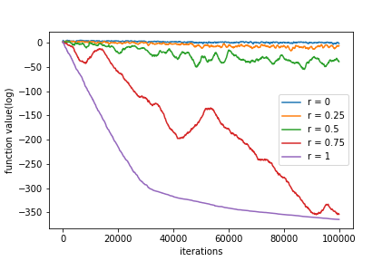
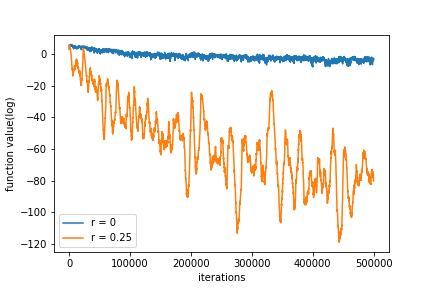
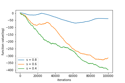
Figure 1: The above figures are for function value with different $r$ and $s$ values, respectively. The left figure plots the performance profiles of Generic Adam with different $r$ values, where $\theta_{t}^{(r)}=1-(0.01+0.99r^{2})/t^{r}$. The middle figure plots the performance profiles of Generic Adam with $\theta_{t}^{(r)}=1-\frac{0.01}{t^{r}}$ and $r=0$ and $0.25$. The right figure plots the performance profiles of Generic Adam with different $s$ values.

In this experiment, we verify the phenomenon described in Section 3.4 how the convergence rate of Generic Adam gradually changes along a continuous path of families of parameters on the one-dimensional counterexample in Chen et al. (2018a):

$$f(x)=\mathbb{E}_{\xi}[\xi x^{2}],$$ (10)

where $\mathbb{P}(\xi=5.5)=1/11$ and $\mathbb{P}(\xi=-0.5)=10/11$.

Sensitivity of parameter $r$.   We set $T=10^{5}$, $\alpha_{t}=5/\sqrt{t}$, $\beta=0.9$, and $\theta_{t}$ as $\theta_{t}^{(r)}=1-(0.01+0.99r^{2})/{t^{r}}$ with $r\in\{0,\ 0.25,\ 0.5,\ 0.75,\ 1.0\}$, respectively. Note that when $r=0$, Generic Adam reduces to the originally divergent Adam (Kingma and Ba, 2014) with $(\beta,\bar{\theta})=(0.9,0.99)$. When $r=1$, Generic Adam reduces to AdaEMA (Chen et al., 2018a) with $\beta=0.9$.

The experimental results are shown in the left figure of Figure 1. We can see that for $r=1.0,0.75$ and $0.5$, Generic Adam is convergent. Moreover, the convergence becomes slower when $r$ decreases, which exactly matches Corollary 10. On the other hand, for $r=0$ and $0.25$, Figure 1 shows that they do not converge. It seems that the divergence for $r=0.25$ contradicts our theory. However, this is because when $r$ is very small, the $\mathcal{O}(T^{-r/4})$ convergence rate is so slow that we may not see a convergent trend in even $10^{5}$ iterations. Indeed, for $r=0.25$, we actually have

$$\theta_{t}^{(0.25)}\leq 1-(0.01+0.25*0.25*0.99)/10^{5*0.25}\approx 0.9960,$$

which is not sufficiently close to 1. As a complementary experiment, we fix the numerator and only change $r$ when $r$ is small. We take $\alpha_{t}$ and $\beta_{t}$ as the same, while $\theta_{t}^{(r)}=1-\frac{0.01}{t^{r}}$ for $r=0$ and $0.25$, respectively. The result is shown in the middle figure of Figures 1. We can see that Generic Adam with $r=0.25$ is indeed convergent in this situation.

Sensitivity of parameter $s$.   Now, we show the sensitivity of $s$ of the sufficient condition (SC) by fixing $r\!=\!0.8$ and selecting $s$ from the collection $s=\{0.4,0.6,0.8\}$. The right figure in Figure 1 illustrates the sensitivity of parameter $s$ when Generic Adam is applied to solve the counterexample (10). The performance shows that when $s$ is fixed, smaller $r$ can lead to a faster and better convergence speed, which also coincides with the convergence results in Corollary 10.

5.2 LeNet on MNIST and ResNet-18 on CIFAR-100

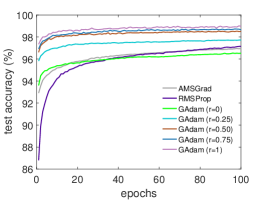
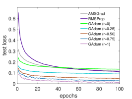
Figure 2: Performance profiles of Generic Adam with $r=\{0,0.25,0.5,0.75,1\}$, RMSProp, and AMSGrad for training LeNet on the MNIST dataset. Figures (a), (b), and (c) illustrate training loss vs. epochs, test accuracy vs. epochs, and test loss vs. epochs, respectively.

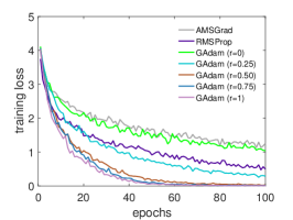
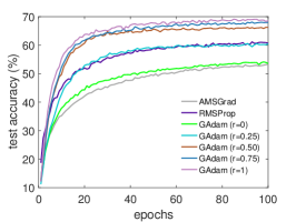
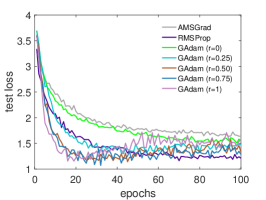
Figure 3: Performance profiles of Generic Adam with $r=\{0,0.25,0.5,0.75,1\}$, RMSProp, and AMSGrad for training ResNet on the CIFAR-100 dataset. Figures (a), (b), and (c) illustrate training loss vs. epochs, test accuracy vs. epochs, and test loss vs. epochs, respectively.

In this subsection, we apply Generic Adam to train LeNet on the MNIST dataset and ResNet-18 on the CIFAR-100 dataset, respectively, to validate the convergence rates in Corollary 10. Meanwhile, the comparisons between Generic Adam and AMSGrad (Reddi et al., 2018; Chen et al., 2018a) are also provided to distinguish their differences in training deep neural networks. We illustrate the performance profiles in three aspects: training loss vs. epochs, test loss vs. epochs, and test accuracy vs. epochs, respectively. MNIST (LeCun et al., 2010) is composed of ten classes of digits among $\{0,1,2,\ldots,9\}$, which includes 60,000 training examples and 10,000 validation examples. The dimension of each example is $28\times 28$. CIFAR-100 (LeCun et al., 2010) is composed of 100 classes of $32\times 32$ color images. Each class includes 6,000 images. Besides, these images are divided into 50,000 training examples and 10,000 validation examples. LetNet (LeCun et al., 1998) used in the experiments is a five-layer convolutional neural network with ReLU activation function whose detailed architecture is described in (LeCun et al., 1998). The batch size is set as $64$. The training stage lasts for $100$ epochs in total. No $\ell_{2}$ regularization on the weights is used. ResNet-18 (He et al., 2016) is a ResNet model containing 18 convolutional layers for CIFAR-100 classification (He et al., 2016). Input images are down-scaled to $1/8$ of their original sizes after the 18 convolutional layers and then fed into a fully-connected layer for the 100-class classification. The output channel numbers of 1-3 conv layers, 4-8 conv layers, 9-13 conv layers, and 14-18 conv layers are $64$, $128$, $256$, and $512$, respectively. The batch size is $64$. The training stage lasts for $100$ epochs in total. No $\ell_{2}$ regularization on the weights is used.

In the experiments, for Generic Adam, we set $\theta_{t}^{(r)}=1-(0.001+0.999r)/t^{r}$ with $r\in\{0,0.25,0.5,0.75,1\}$ and $\beta_{t}=0.9$, respectively; for RMSProp, we set $\beta_{t}=0$ and $\theta_{t}=1-\frac{1}{t}$ along with the parameter settings in Mukkamala and Hein (2017). For fairness, the base learning rates $\alpha_{t}$ in Generic Adam, RMSProp, and AMSGrad are all set as $0.001/\sqrt{t}$. Figures 3 and 3 illustrate the results of Generic Adam with different $r$, RMSProp, and AMSGrad for training LeNet on MNIST and training ResNet-18 on CIFAR-100, respectively. We can see that AMSGrad and Adam (Generic Adam with $r=0$) decrease the training loss slowest and show the worst test accuracy among the compared optimizers. One possible reason is due to the use of constant $\theta$ in AMSGrad and original Adam. By Figures 3 and 3, we can observe that the convergences of Generic Adam are extremely sensitive to the choice of parameter $\theta_{t}$. Larger $r$ can contribute to a faster convergence rate of Generic Adam, which corroborates the theoretical result in Corollary 10. Additionally, the test accuracies in Figures 3(b) and 3(b) indicate that a smaller training loss can contribute to a higher test accuracy for Generic Adam.

5.3 Experiments on Practical Adam

5.3.1 Ablation Study between Batchsize and Optimal Learning Rate

In this section, we apply mini-batch Adam algorithms and mini-batch SGD algorithms to the following quadratic minimization task:

$$\min_{x}\mathbb{E}_{\xi\sim\mathcal{N}(0,100I)}\left[x^{T}Ax-b^{T}x+\xi^{T}x\right],$$

where, for simplicity, $A\in\mathbb{R}^{3\times 3}$ and $b\in\mathbb{R}^{3}$. We optimize $x$ with batch size 1 to 320, and grid search the best learning rate from $\{k/2000|k=1,2,\cdots,2000\}$. For each pair of batch size and learning rate, we randomly sample 500 trials and take the average gradient norm as the criteria. Fig. 4 shows the result of the best learning rate and averaged gradient norm for different batch sizes after 200 optimization iterations. From the figure, we can verify that when the batch size becomes larger, the optimal learning rate for SGD and SGD-momentum increases a lot (from 0.005 to 0.04). Meanwhile, with the adaptive learning rate, the optimal learning rate does not change too much (between 0.02 to 0.04). Hence, it shows the benefit of adaptive learning rate methods compared to SGD and verifies Remark 18.

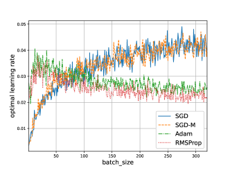
Figure 4: Performance profiles of optimal learning rate v.s. batch size and optimality gap v.s. batch size.

5.3.2 Vision Tasks

In this section we apply the mini-batch Adam algorithm to train LeNet on the MNIST dataset and ResNet-18 on the CIFAR-100 dataset. Datasets and network architecture are the same as they are described in Section 5.2. But instead of using $\alpha_{t}=\alpha/\sqrt{t}$, $\theta_{t}=1-\theta/t$, we set $\beta_{t}=0.9$ and $\theta_{t}=0.99$ for Adam and AMSGrad, and set $\beta_{t}=0.9$ for RMSProp. We use different batchsizes {32, 64, 128} to train networks. Besides, when training ResNet-18 on the CIFAR100 dataset, we use an $\ell_{2}$ regularization on weights, the coefficient of the regularization term to $5e-4$. We use grid search in $[1e-2,\ 5e-3,\ 1e-3,\ 5e-4,\ 1e-4]$ for $\alpha_{t}$ with respect to test accuracy. In addition, when training ResNet-18 on the CIFAR100 dataset, $\alpha_{t}$ will reduce to $0.2\times\alpha_{t}$ every 19550 iterations (50 epochs for the 128 batchsize setting), which (learning rate decay) is commonly used in practice . The experimental results are shown in Figure 5 and Figure 6. It can be shown that larger batchsize can give lower training loss in all experiments. However, large batchsize for training does not imply higher test accuracy or lower test loss, which needs to be further explored and examined.

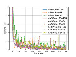
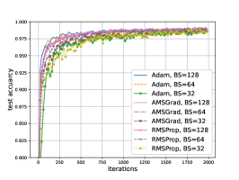
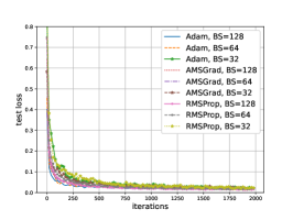
Figure 5: Performance profiles of mini-batch Adam, RMSProp and AMSGrad on MNIST, with batchsize = $\{32,\ 64,\ 128\}$.

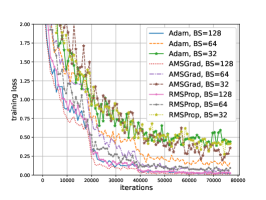
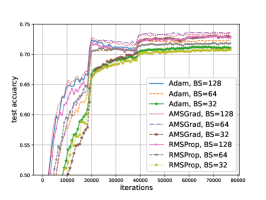
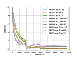
Figure 6: Performance profiles of mini-batch Adam, RMSProp and AMSGrad on CIFAR100, with batchsize = $\{32,\ 64,\ 128\}$.

5.3.3 Transformer XL on WikiText-103

Also, we applied mini-batch Adam to train a base model of Transformer XL (Dai et al., 2019) on the dataset WikiText-103 (Merity et al., 2016). The base model of Transformer XL contains 16 self-attention layers. In each self-attention layer, there are 10 heads, and the encoding dimension of each head is set to 41. The WikiText-103 dataset is a collection of over 100 million tokens extracted from the set of verified ‘Good’ and ‘Featured’ articles on Wikipedia. We adopt the same parameter settings provided by the authors but test on batch size $\{30,60,120\}$. The results are shown in Figure 7. Also, as it is shown in the figure, a larger batch size can give a lower training loss in all experiments. Meanwhile, in the figure, AMSGrad and Adam achieve much better performance than SGD-M, which shows the benefit of using adaptive methods instead of SGD-based methods, just like what was mentioned in Zhang et al. (2019).

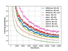
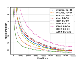
Figure 7: Performance profiles of mini-batch Adam, SGD-M and AMSGrad on WikiText-103, with batchsize = $\{30,\ 60,\ 120\}$.

6 Conclusions

In this work, we delved into the convergences of Adam, and presented an easy-to-check sufficient condition to guarantee their convergences in the non-convex stochastic setting. This sufficient condition merely depends on the base learning rate and the linear combination parameter of second-order moments. Relying on this sufficient condition, we found that the divergences of Adam are possibly due to the incorrect parameter settings. Besides, when encountering the practice Adam, we theoretically showed that the number of samples will linearly speed up the convergence in both the mini-batch setting and distributed setting, which closes the gap between theory and practice. At last, the correctness of theoretical results has also been verified via the counterexample and training deep neural networks on real-world datasets.

Appendix A Key Lemma to prove Theorem 2 and Theorem 13

In this section we provide the necessary lemmas for the proofs of Theorem 2 and Theorem 13. First, we give some notations for simplifying the following proof.

Notations

We use bold letters to represent vectors. The $k$-th component of a vector $\bm{v}_{t}$ is denoted as ${v}_{t,k}$. The inner product between two vectors $\bm{v}_{t}$ and $\bm{w}_{t}$ is denoted as $\langle\bm{v}_{t},\bm{w}_{t}\rangle$. Other than that, all computations that involve vectors shall be understood in the component-wise way. We say a vector $\bm{v}_{t}\geq 0$ if every component of $\bm{v}_{t}$ is non-negative, and $\bm{v}_{t}\geq\bm{w}_{t}$ if $v_{t,k}\geq w_{t,k}$ for all $k=1,2,\ldots,d$. The $\ell_{1}$ norm of a vector $\bm{v}_{t}$ is defined as $\left\|\bm{v}_{t}\right\|_{1}=\sum_{k=1}^{d}|{v}_{t,k}|$. The $\ell_{2}$ norm is defined as $\left\|\bm{v}_{t}\right\|^{2}=\langle\bm{v}_{t},\bm{v}_{t}\rangle=\sum_{k=1}^{d}|{v}_{t,k}|^{2}$. Given a positive vector $\bm{\hat{\eta}}_{t}$, it will be helpful to define the following weighted norm: $\left\|\bm{v}_{t}\right\|^{2}_{\bm{\eta}_{t}}=\langle\bm{v}_{t},\bm{\hat{\eta}}_{t}\bm{v}_{t}\rangle=\sum_{k=1}^{d}\hat{\eta}_{t,k}|{v}_{t,k}|^{2}$.

Lemma 24.

Given $S_{0}>0$ and a non-negative sequence $\{s_{t}\}$, let $S_{t}=S_{0}+\sum_{i=1}^{t}s_{i}$ for $t\geq 1$. Then the following estimate holds

$$\sum_{t=1}^{T}\frac{s_{t}}{S_{t}}\leq\log(S_{T})-\log(S_{0}).$$ (11)

Proof  The finite sum $\sum_{t=1}^{T}{s_{t}}/{S_{t}}$ can be interpreted as a Riemann sum $\sum_{t=1}^{T}(S_{t}-S_{t-1})/S_{t}.$ Since $1/x$ is decreasing on the interval $(0,\infty)$, we have

$$\sum_{t=1}^{T}\frac{S_{t}-S_{t-1}}{S_{t}}\leq\int_{S_{0}}^{S_{T}}\frac{1}{x}dx=\log(S_{T})-\log(S_{0}).$$

The proof is completed.  

Lemma 25 (Abel’s Lemma - Summation by parts).

Let $\{u_{t}\}$ and $\{s_{t}\}$ be two non-negative sequences. Let $S_{t}=\sum_{i=1}^{t}s_{i}$ for $t\geq 1$. Then

$$\sum_{t=1}^{T}u_{t}s_{t}=\sum_{t=1}^{T-1}(u_{t}-u_{t+1})S_{t}+u_{T}S_{T}.$$ (12)

Proof  Let $S_{0}=0$. Then

$$\sum_{t=1}^{T}u_{t}s_{t}=\sum_{t=1}^{T}u_{t}(S_{t}-S_{t-1})=\sum_{t=1}^{T-1}u_{t}S_{t}-\sum_{t=1}^{T-1}u_{t+1}S_{t}+u_{T}S_{T}=\sum_{t=1}^{T-1}(u_{t}-u_{t+1})S_{t}+u_{T}S_{T}.$$ (13)

The proof is completed.  

Lemma 26.

Let $\{\theta_{t}\}$ and $\{\alpha_{t}\}$ satisfy the restrictions (R2) and (R3). For any $i\leq t$, we have

$$\chi_{t}\leq C_{0}\chi_{i}\text{~{}~{}and~{}~{}}\alpha_{t}\leq C_{0}\alpha_{i}.$$ (14)

Proof  For any $i\leq t$, since the sequence $\{a_{t}\}$ is non-increasing, we have $a_{t}\leq a_{i}$. Hence,

$$\chi_{t}=\frac{\alpha_{t}}{\sqrt{1-\theta_{t}}}\leq C_{0}a_{t}\leq C_{0}a_{i}\leq C_{0}\frac{\alpha_{i}}{\sqrt{1-\theta_{i}}}=C_{0}\chi_{i},$$

which proves the first inequality. On the other hand, since $\{\theta_{t}\}$ is non-decreasing, it holds

$$\alpha_{t}\leq C_{0}\frac{\sqrt{1-\theta_{t}}}{\sqrt{1-\theta_{i}}}\alpha_{i}\leq C_{0}\alpha_{i}=C_{0}\alpha_{i}.$$

The proof is completed.  

Let $\Theta_{(t,i)}=\prod_{j=i+1}^{t}\theta_{j}$ for $i<t$ and $\Theta_{(t,t)}=1$ by convention.

Lemma 27.

Fix a constant $\theta^{\prime}$ with $\beta^{2}<\theta^{\prime}<\theta$. Let $C_{1}$ be as given as Eq. (6) in the main paper. For any $i\leq t$, we have

$$\Theta_{(t,i)}\geq C_{1}(\theta^{\prime})^{t-i}.$$ (15)

Proof  For any $i\leq t$, since $\theta_{j}\geq\theta^{\prime}$ for $j\geq N$, and $\theta_{j}<\theta^{\prime}$ for $j<N$, we have

$$\Theta_{(t,i)}=\prod_{j=i+1}^{t}\theta_{j}\geq\left(\prod_{j=i+1}^{N}\theta_{j}\right)(\theta^{\prime})^{t-N}=\left(\prod_{j=i+1}^{N}({\theta_{j}}/{\theta^{\prime}})\right)(\theta^{\prime})^{t-i}\geq\left(\prod_{j=1}^{N}({\theta_{j}}/{\theta^{\prime}})\right)(\theta^{\prime})^{t-i}.$$

We take the constant $C_{1}=\prod_{j=1}^{N}(\theta_{j}/\theta^{\prime})$, where $N$ is the maximum of the indices for which $\theta_{j}<\theta^{\prime}$. The proof is completed.  

Remark 28.

If $\theta_{t}=\theta$ is a constant, we have $\Theta_{(t,i)}=\theta^{t-i}$. In this case we can take $\theta^{\prime}=\theta$ and $C_{1}=1$.

Lemma 29.

Let $\gamma:=\beta^{2}/{\theta^{\prime}}$. We have the following estimate

$$\bm{m_{t}}^{2}\leq\frac{1}{C_{1}(1-\gamma)(1-\theta_{t})}\bm{v}_{t},~{}\forall t.$$ (16)

Proof  Let $B_{(t,i)}=\prod_{j=i+1}^{t}\beta_{j}$ for $i<t$ and $B_{(t,t)}=1$ by convention. By the iteration formula $\bm{m}_{t}=\beta_{t}\bm{m}_{t-1}+(1-\beta_{t})\bm{g}_{t}$ and $\bm{m}_{0}=\bm{0}$, we have

$$\bm{m}_{t}=\sum_{i=1}^{t}\left(\prod_{j=i+1}^{t}\beta_{j}\right)(1-\beta_{i})\bm{g}_{i}=\sum_{i=1}^{t}B_{(t,i)}(1-\beta_{i})\bm{g}_{i}.$$

Similarly, by $\bm{v}_{t}=\theta_{t}\bm{v}_{t-1}+(1-\theta_{t})\bm{g}_{t}^{2}$ and $\bm{v}_{0}=\bm{\epsilon}$, we have

$$\bm{v}_{t}=\left(\prod_{j=1}^{t}\theta_{j}\right)\bm{\epsilon}+\sum_{i=1}^{t}\left(\prod_{j=i+1}^{t}\theta_{j}\right)\left({1-\theta_{i}}\right)\bm{g}_{i}^{2}\geq\sum_{i=1}^{t}\Theta_{(t,i)}(1-\theta_{i})\bm{g}_{i}^{2}.$$

It follows by arithmetic inequality that

$$\begin{split}\bm{m}_{t}^{2}&=\left(\sum_{i=1}^{t}\frac{(1-\beta_{i})B_{(t,i)}}{\sqrt{(1-\theta_{i})\Theta_{(t,i)}}}\sqrt{(1-\theta_{i})\Theta_{(t,i)}}\bm{g}_{i}\right)^{2}\\ &\leq\left(\sum_{i=1}^{t}\frac{(1-\beta_{i})^{2}B_{(t,i)}^{2}}{(1-\theta_{i})\Theta_{(t,i)}}\right)\left(\sum_{i=1}^{t}\Theta_{(t,i)}(1-\theta_{i})\bm{g}_{i}^{2}\right)\leq\left(\sum_{i=1}^{t}\frac{(1-\beta_{i})^{2}B_{(t,i)}^{2}}{(1-\theta_{i})\Theta_{(t,i)}}\right)\bm{v}_{t}.\end{split}$$

Note that $\{\theta_{t}\}$ is non-decreasing by (R2), and $B_{(t,i)}\leq\beta^{t-i}$ by (R1). By Lemma 27, we have

$$\sum_{i=1}^{t}\frac{(1-\beta_{i})^{2}B_{(t,i)}^{2}}{(1-\theta_{i})\Theta_{(t,i)}}\leq\frac{1}{C_{1}(1-\theta_{t})}\sum_{i=1}^{t}\left(\frac{\beta^{2}}{\theta^{\prime}}\right)^{t-i}\leq\frac{1}{C_{1}(1-\theta_{t})}\sum_{k=0}^{t-1}\gamma^{k}\leq\frac{1}{C_{1}(1-\gamma)(1-\theta_{t})}.$$

The proof is completed.  

Let $\bm{\Delta}_{t}:=\bm{x}_{t+1}-\bm{x}_{t}=-\alpha_{t}\bm{m}_{t}/\sqrt{\bm{v}_{t}}$. Let $\bm{\hat{v}}_{t}=\theta_{t}\bm{v}_{t-1}+(1-\theta_{t})\bm{\delta_{t}}^{2}$, where $\bm{\delta_{t}}^{2}=\mathbb{E}_{t}\left[\bm{g}_{t}^{2}\right]$ and let $\bm{\hat{\eta}_{t}}=\alpha_{t}/\sqrt{\bm{\hat{v}_{t}}}$.

Lemma 30.

With the notations above, the following equality holds

$$\begin{split}\bm{\Delta}_{t}-\frac{\beta_{t}\alpha_{t}}{\sqrt{\theta_{t}}\alpha_{t-1}}\bm{\Delta}_{t-1}=-(1-\beta_{t})\bm{\hat{\eta}}_{t}\bm{g}_{t}+\bm{\hat{\eta}}_{t}\bm{g}_{t}\frac{(1-\theta_{t})\bm{g}_{t}}{\sqrt{\bm{v}}_{t}}\bm{A}_{t}+\bm{\hat{\eta}}_{t}\bm{\delta}_{t}\frac{(1-\theta_{t})\bm{g}_{t}}{\sqrt{\bm{v}_{t}}}\bm{B}_{t},\end{split}$$ (17)

where

$$\begin{split}\bm{A}_{t}&=\frac{\beta_{t}\bm{m}_{t-1}}{\sqrt{\bm{v}_{t}}+\sqrt{\theta_{t}\bm{v}_{t-1}}}+\frac{(1-\beta_{t})\bm{g}_{t}}{\sqrt{\bm{v}}_{t}+\sqrt{\bm{\hat{v}}_{t}}},\\ \bm{B}_{t}&=\left(\frac{\beta_{t}\bm{m}_{t-1}}{\sqrt{\theta_{t}\bm{v}_{t-1}}}\frac{\sqrt{1-\theta_{t}}\bm{g}_{t}}{\sqrt{\bm{v}}_{t}+\sqrt{\theta_{t}\bm{v}_{t-1}}}\frac{\sqrt{1-\theta_{t}}\bm{\delta}_{t}}{\sqrt{\bm{\hat{v}}_{t}}+\sqrt{\theta_{t}\bm{v}_{t-1}}}\right)-\frac{(1-\beta_{t})\bm{\delta}_{t}}{\sqrt{\bm{v}_{t}}+\sqrt{\bm{\hat{v}}_{t}}}.\end{split}$$

Proof  We have

$$\begin{split}\bm{\Delta}_{t}-\frac{\beta_{t}\alpha_{t}}{\sqrt{\theta_{t}}\alpha_{t-1}}\bm{\Delta}_{t-1}=~{}&-\frac{\alpha_{t}\bm{m_{t}}}{\sqrt{\bm{v}_{t}}}+\frac{\beta_{t}\alpha_{t}\bm{m}_{t-1}}{\sqrt{\theta_{t}\bm{v}_{t-1}}}=-\alpha_{t}\left(\frac{\bm{m}_{t}}{\sqrt{\bm{v}_{t}}}-\frac{\beta_{t}\bm{m}_{t-1}}{\sqrt{\theta_{t}\bm{v}_{t-1}}}\right)\\ =~{}&-\underbrace{\frac{(1-\beta_{t})\alpha_{t}\bm{g}_{t}}{\sqrt{\bm{v}_{t}}}}_{\text{(I)}}+\underbrace{\beta_{t}\alpha_{t}\bm{m}_{t-1}\left(\frac{1}{\sqrt{\theta_{t}\bm{v}_{t-1}}}-\frac{1}{\sqrt{\bm{v}_{t}}}\right)}_{\text{(II)}}.\end{split}$$ (18)

For (I) we have

$$\begin{split}\text{(I)}=~{}&\frac{(1-\beta_{t})\alpha_{t}\bm{g}_{t}}{\sqrt{\bm{\hat{v}}}_{t}}+(1-\beta_{t})\alpha_{t}\bm{g}_{t}\left(\frac{1}{\sqrt{\bm{v}}_{t}}-\frac{1}{\sqrt{\bm{\hat{v}}_{t}}}\right)\\ =~{}&(1-\beta_{t})\bm{\hat{\eta}}_{t}\bm{g}_{t}+(1-\beta_{t})\alpha_{t}\bm{g}_{t}\frac{(1-\theta_{t})(\bm{\delta}_{t}^{2}-\bm{g}_{t}^{2})}{\sqrt{\bm{v}_{t}}\sqrt{\bm{\hat{v}}_{t}}(\sqrt{\bm{v}_{t}}+\sqrt{\bm{\hat{v}}_{t}})}\\ =~{}&(1-\beta_{t})\bm{\hat{\eta}}_{t}\bm{g}_{t}+\bm{\hat{\eta}}_{t}\bm{\delta}_{t}\frac{(1-\theta_{t})\bm{g}_{t}}{\sqrt{\bm{v}_{t}}}\frac{(1-\beta_{t})\bm{\delta}_{t}}{\sqrt{\bm{v}_{t}}+\sqrt{\bm{\hat{v}}_{t}}}-\bm{\hat{\eta}}_{t}\bm{g}_{t}\frac{(1-\theta_{t})\bm{g}_{t}}{\sqrt{\bm{v}_{t}}}\frac{(1-\beta_{t})\bm{g}_{t}}{\sqrt{\bm{v}_{t}}+\sqrt{\bm{\hat{v}}}_{t}}.\end{split}$$ (19)

For (II) we have

$$\begin{split}\text{(II)}&=\beta_{t}\alpha_{t}\bm{m}_{t-1}\frac{(1-\theta_{t})\bm{g}_{t}^{2}}{\sqrt{\bm{v}_{t}}\sqrt{\theta_{t}\bm{v}_{t-1}}(\sqrt{\bm{v}_{t}}+\sqrt{\theta_{t}\bm{v}_{t-1}})}\\ &=\beta_{t}\alpha_{t}\bm{m}_{t-1}\frac{(1-\theta_{t})\bm{g}_{t}^{2}}{\sqrt{\bm{v}_{t}}\sqrt{\bm{\hat{v}}_{t}}(\sqrt{\bm{v}_{t}}+\sqrt{\theta_{t}\bm{v}_{t-1}})}+\beta_{t}\alpha_{t}\bm{m}_{t-1}\frac{(1-\theta_{t})\bm{g}_{t}^{2}}{\sqrt{\bm{v}_{t}}(\sqrt{\bm{v}_{t}}+\sqrt{\theta_{t}\bm{v}_{t-1}})}\left(\frac{1}{\sqrt{\theta_{t}\bm{v}_{t-1}}}-\frac{1}{\sqrt{\bm{\hat{v}}_{t}}}\right)\\ &=\bm{\hat{\eta}}_{t}\bm{g}_{t}\frac{(1-\theta_{t})\bm{g}_{t}}{\sqrt{\bm{v}_{t}}}\left(\frac{\beta_{t}\bm{m}_{t-1}}{\sqrt{\bm{v}_{t}}+\sqrt{\theta_{t}\bm{v}_{t-1}}}\right)+\frac{\beta_{t}\alpha_{t}\bm{m}_{t-1}(1-\theta_{t})^{2}\bm{g}_{t}^{2}\bm{\delta}_{t}^{2}}{\sqrt{\bm{v}_{t}}\sqrt{\bm{\hat{v}}_{t}}\sqrt{\theta_{t}\bm{v}_{t-1}}(\sqrt{\bm{v}_{t}}+\sqrt{\theta_{t}\bm{v}_{t-1}})(\sqrt{\bm{\hat{v}}_{t}}+\sqrt{\theta_{t}\bm{v}_{t-1}})}\\ &=\bm{\hat{\eta}}_{t}\bm{g}_{t}\frac{(1-\theta_{t})\bm{g}_{t}}{\sqrt{\bm{v}_{t}}}\left(\frac{\beta_{t}\bm{m}_{t-1}}{\sqrt{\bm{v}_{t}}+\sqrt{\theta_{t}\bm{v}_{t-1}}}\right)+\bm{\hat{\eta}}_{t}\bm{\delta}_{t}\frac{(1-\theta_{t})\bm{g}_{t}}{\sqrt{\bm{v}_{t}}}\left(\frac{\beta_{t}\bm{m}_{t-1}}{\sqrt{\theta_{t}\bm{v}_{t-1}}}\frac{\sqrt{1-\theta_{t}}\bm{g}_{t}}{\sqrt{\bm{v}}_{t}+\sqrt{\theta_{t}\bm{v}_{t-1}}}\frac{\sqrt{1-\theta_{t}}\bm{\delta}_{t}}{\sqrt{\bm{\hat{v}}_{t}}+\sqrt{\theta_{t}\bm{v}_{t-1}}}\right).\end{split}$$ (20)

Combining Eq. (19) and Eq. (20), we obtain the desired Eq. (17). The proof is completed.  

Lemma 31.

Let $M_{t}=\mathbb{E}\left[\left\langle\bm{\nabla}f(\bm{x}_{t}),\bm{\Delta}_{t}\right\rangle+L\left\|\bm{\Delta}_{t}\right\|^{2}\right]$ and $\chi_{t}={\alpha_{t}}/{\sqrt{1-\theta_{t}}}$. Then for any $t\geq 2$, we have

$$\begin{split}M_{t}\leq&\frac{\beta_{t}\alpha_{t}}{\sqrt{\theta_{t}}\alpha_{t-1}}M_{t-1}+L\ \mathbb{E}\left[\left\|\bm{\Delta}_{t}\right\|^{2}\right]+C_{2}G\chi_{t}\mathbb{E}\left[\left\|\frac{\sqrt{1-\theta_{t}}\bm{g}_{t}}{\sqrt{\bm{v}_{t}}}\right\|^{2}\right]-\frac{1-\beta}{2}\mathbb{E}\left[\left\|\bm{\nabla}f(\bm{x}_{t})\right\|^{2}_{\bm{\hat{\eta}}_{t}}\right]\end{split}$$ (21)

and

$$M_{1}\leq L\ \mathbb{E}\left[\left\|\bm{\Delta}_{1}\right\|^{2}\right]+C_{2}G\chi_{1}\mathbb{E}\left[\left\|\frac{\sqrt{1-\theta_{t}}\bm{g}_{1}}{\sqrt{v}_{1}}\right\|^{2}\right],$$ (22)

where $C_{2}=2\left(\frac{\beta/(1-\beta)}{\sqrt{C_{1}(1-\gamma)\theta_{1}}}+1\right)^{2}$.

Proof  First, for $t\geq 2$ we have

$$\begin{split}\mathbb{E}\langle\bm{\nabla}f(\bm{x}_{t}),\bm{\Delta}_{t}\rangle=\underbrace{\frac{\beta_{t}\alpha_{t}}{\sqrt{\theta_{t}}\alpha_{t-1}}\mathbb{E}\langle\bm{\nabla}f(\bm{x}_{t}),\bm{\Delta}_{t-1}\rangle}_{\text{(I)}}+\underbrace{\mathbb{E}\left\langle\bm{\nabla}f(\bm{x}_{t}),\bm{\Delta}_{t}-\frac{\beta_{t}\alpha_{t}}{\sqrt{\theta_{t}}\alpha_{t-1}}\bm{\Delta}_{t-1}\right\rangle}_{\text{(II)}}.\end{split}$$ (23)

To estimate (I), by the Schwartz inequality and the Lipschitz continuity of the gradient of $f$, we have

$$\begin{split}\langle\bm{\nabla}f(\bm{x}_{t}),\bm{\Delta}_{t-1}\rangle\leq~{}&\langle\bm{\nabla}f(\bm{x}_{t-1}),\bm{\Delta}_{t-1}\rangle+\langle\bm{\nabla}f(\bm{x}_{t})-\bm{\nabla}f(\bm{x}_{t-1}),\bm{\Delta}_{t-1}\rangle\\ \leq~{}&\langle\bm{\nabla}f(\bm{x}_{t-1}),\bm{\Delta}_{t-1}\rangle+L\left\|\bm{x}_{t}-\bm{x}_{t-1}\right\|\left\|\bm{\Delta}_{t-1}\right\|\\ =~{}&\langle\bm{\nabla}f(\bm{x}_{t-1}),\bm{\Delta}_{t-1}\rangle+L\left\|\bm{\Delta}_{t-1}\right\|^{2}.\\ \end{split}$$ (24)

Hence, we have

$$\text{(I)}\leq\frac{\beta_{t}\alpha_{t}}{\sqrt{\theta_{t}}\alpha_{t-1}}\mathbb{E}\left[\langle\bm{\nabla}f(\bm{x}_{t-1}),\bm{\Delta}_{t-1}\rangle+L\left\|\bm{\Delta}_{t-1}\right\|^{2}\right]=\frac{\beta_{t}\alpha_{t}}{\sqrt{\theta_{t}}\alpha_{t-1}}M_{t-1}.$$ (25)

To estimate (II), by Lemma 30, we have

$$\begin{split}&\mathbb{E}\left\langle\bm{\nabla}f(\bm{x}_{t}),\bm{\Delta}_{t}-\frac{\beta_{t}\alpha_{t}}{\sqrt{\theta_{t}}\alpha_{t-1}}\bm{\Delta}_{t-1}\right\rangle\\ =&-(1-\beta_{t})\mathbb{E}\langle\bm{\nabla}f(\bm{x}_{t}),\bm{\hat{\eta}}_{t}\bm{g}_{t}\rangle\underbrace{-\mathbb{E}\left\langle\bm{\nabla}f(\bm{x}_{t}),\bm{\hat{\eta}}_{t}\bm{g}_{t}\frac{(1-\theta_{t})\bm{g}_{t}}{\sqrt{\bm{v}}_{t}}\bm{A}_{t}\right\rangle}_{\text{(III)}}\underbrace{-\mathbb{E}\left\langle\bm{\nabla}f(\bm{x}_{t}),\bm{\hat{\eta}}_{t}\bm{\delta}_{t}\frac{(1-\theta_{t})\bm{g}_{t}}{\sqrt{\bm{v}}_{t}}\bm{B}_{t}\right\rangle}_{\text{(IV)}}.\end{split}$$ (26)

Note that $\bm{\hat{\eta}}_{t}$ is independent of $\bm{g}_{t}$ and $\mathbb{E}_{t}[\bm{g}_{t}]=\bm{\nabla}f(\bm{x}_{t})$. Hence, for the first term in the right hand side of Eq. (26), we have

$$\begin{split}-(1-\beta_{t})\mathbb{E}\langle\bm{\nabla}f(\bm{x}_{t}),\bm{\hat{\eta}}_{t}\bm{g}_{t}\rangle&=-(1-\beta_{t})\mathbb{E}\left\langle\bm{\nabla}f(\bm{x}_{t}),\bm{\hat{\eta}}_{t}\mathbb{E}_{t}[\bm{g}_{t}]\right\rangle\\ &=-(1-\beta_{t})\mathbb{E}\left\|\bm{\nabla}f(\bm{x}_{t})\right\|^{2}_{\bm{\hat{\eta}}_{t}}\\ &\leq-(1-\beta)\mathbb{E}\left\|\bm{\nabla}f(\bm{x}_{t})\right\|^{2}_{\bm{\hat{\eta}}_{t}}.\end{split}$$ (27)

To estimate (III), we have

$$\begin{split}\text{(III)}~{}\leq\mathbb{E}\left\langle\frac{\sqrt{\bm{\hat{\eta}}_{t}}|\bm{\nabla}f(\bm{x}_{t})||\bm{g}_{t}|}{\bm{\delta}_{t}},\frac{\sqrt{\bm{\hat{\eta}}_{t}}\bm{\delta}_{t}|\bm{A}_{t}|(1-\theta_{t})|\bm{g}_{t}|}{\sqrt{\bm{v}_{t}}}\right\rangle.\end{split}$$ (28)

Note that $\bm{\delta}_{t}\leq G$. Therefore,

$$\sqrt{\bm{\hat{\eta}}_{t}}\bm{\delta}_{t}=\sqrt{\bm{\hat{\eta}}_{t}\bm{\delta}_{t}^{2}}=\sqrt{\frac{\alpha_{t}\bm{\delta}_{t}^{2}}{\sqrt{\bm{\hat{v}}_{t}}}}\leq\sqrt{\frac{\alpha_{t}\bm{\delta}_{t}^{2}}{\sqrt{(1-\theta_{t})\bm{\delta}_{t}^{2}}}}\leq\sqrt{\frac{G\alpha_{t}}{\sqrt{1-\theta_{t}}}}=\sqrt{G\chi_{t}}.$$ (29)

On the other hand,

$$\begin{split}|\bm{A}_{t}|=\left|\frac{\beta_{t}\bm{m}_{t-1}}{\sqrt{\bm{v}_{t}}+\sqrt{\theta_{t}\bm{v}_{t-1}}}+\frac{(1-\beta_{t})\bm{g}_{t}}{\sqrt{\bm{v}}_{t}+\sqrt{\bm{\hat{v}}_{t}}}\right|\leq\frac{\beta_{t}|\bm{m}_{t-1}|}{\sqrt{\theta_{t}\bm{v}_{t-1}}}+\frac{(1-\beta_{t})|\bm{g}_{t}|}{\sqrt{\bm{v}_{t}}}.\end{split}$$ (30)

By Lemma 29, we have

$$\frac{|\bm{m}_{t-1}|}{\sqrt{\bm{v}_{t-1}}}\leq\frac{1}{\sqrt{C_{1}(1-\gamma)(1-\theta_{t})}}.$$ (31)

Meanwhile,

$$\frac{|\bm{g}_{t}|}{\sqrt{\bm{v}_{t}}}\leq\frac{|\bm{g}_{t}|}{\sqrt{(1-\theta_{t})\bm{g}_{t}^{2}}}=\frac{1}{\sqrt{1-\theta_{t}}}.$$ (32)

Hence, we have

$$\begin{split}|\bm{A}_{t}|&\leq\frac{\beta_{t}}{\sqrt{C_{1}(1-\gamma)(1-\theta_{t})\theta_{t}}}+\frac{1-\beta_{t}}{\sqrt{1-\theta_{t}}}\leq\left(\frac{\beta_{t}/(1-\beta_{t})}{\sqrt{C_{1}(1-\gamma)\theta_{t}}}+1\right)\frac{1-\beta_{t}}{\sqrt{1-\theta_{t}}}\\ &\leq\left(\frac{\beta/(1-\beta)}{\sqrt{C_{1}(1-\gamma)\theta_{1}}}+1\right)\frac{1-\beta_{t}}{\sqrt{1-\theta_{t}}}:=\frac{C_{2}^{\prime}(1-\beta_{t})}{\sqrt{1-\theta_{t}}},\end{split}$$ (33)

where $C_{2}^{\prime}=\left(\frac{\beta/(1-\beta)}{\sqrt{C_{1}(1-\gamma)\theta_{1}}}+1\right)$. The last inequality holds due to $\beta_{t}/(1-\beta_{t})\leq\beta/(1-\beta)$ as $\beta_{t}\leq\beta$. Therefore, we have

$$\begin{split}&\left\langle\frac{\sqrt{\bm{\hat{\eta}}_{t}}|\bm{\nabla}f(\bm{x}_{t})||\bm{g}_{t}|}{\bm{\delta}_{t}},\frac{\sqrt{\bm{\hat{\eta}}_{t}}\bm{\delta}_{t}|\bm{A}_{t}|(1-\theta_{t})|\bm{g}_{t}|}{\sqrt{\bm{v}_{t}}}\right\rangle\\ \leq~{}&\left\langle\frac{\sqrt{\bm{\hat{\eta}}_{t}}|\bm{\nabla}f(\bm{x}_{t})||\bm{g}_{t}|}{\bm{\delta}_{t}},\sqrt{G\chi_{t}}C_{2}^{\prime}(1-\beta_{t})\frac{\sqrt{1-\theta_{t}}|\bm{g}_{t}|}{\sqrt{\bm{v}_{t}}}\right\rangle\\ \leq~{}&\frac{1-\beta_{t}}{4}\left\|\frac{\sqrt{\bm{\hat{\eta}}_{t}}|\bm{\nabla}f(\bm{x}_{t})||\bm{g}_{t}|}{\bm{\delta}_{t}}\right\|^{2}+{C_{2}^{\prime 2}G}{(1-\beta_{t})}\chi_{t}\left\|\frac{\sqrt{1-\theta_{t}}\bm{g}_{t}}{\sqrt{\bm{v}_{t}}}\right\|^{2}\\ \leq~{}&\frac{1-\beta_{t}}{4}\left\|\frac{\bm{\hat{\eta}}_{t}|\bm{\nabla}f(\bm{x}_{t})|^{2}|\bm{g}_{t}|^{2}}{\bm{\delta}_{t}^{2}}\right\|_{1}+{C_{2}^{\prime 2}G}\chi_{t}\left\|\frac{\sqrt{1-\theta_{t}}\bm{g}_{t}}{\sqrt{\bm{v}_{t}}}\right\|^{2}.\end{split}$$ (34)

Note that $\bm{\delta}_{t}^{2}=\mathbb{E}_{t}[\bm{g}_{t}^{2}]$. Hence,

$$\mathbb{E}_{t}\left\|\frac{\bm{\hat{\eta}}_{t}|\bm{\nabla}f(\bm{x}_{t})|^{2}|\bm{g}_{t}|^{2}}{\bm{\delta}_{t}^{2}}\right\|_{1}=\left\|\bm{\hat{\eta}}_{t}|\bm{\nabla}f(\bm{x}_{t})|^{2}\right\|_{1}=\left\|\bm{\nabla}f(\bm{x}_{t})\right\|_{\bm{\hat{\eta}}_{t}}^{2}.$$ (35)

Combining Eq. (28), Eq. (34), and Eq. (35), we obtain

$$\begin{split}\text{(III)}\leq~{}&\frac{1-\beta_{t}}{4}\mathbb{E}\left[\left\|\bm{\nabla}f(\bm{x}_{t})\right\|_{\bm{\hat{\eta}}_{t}}^{2}\right]+{C_{2}^{\prime 2}G}\chi_{t}\mathbb{E}\left\|\frac{\sqrt{1-\theta_{t}}\bm{g}_{t}}{\sqrt{\bm{v}_{t}}}\right\|^{2}.\end{split}$$ (36)

The term (IV) is estimated similarly as term (III). First, we have

$$\begin{split}|\bm{B}_{t}|\leq~{}&\left(\frac{\beta_{t}|\bm{m}_{t-1}|}{\sqrt{\theta_{t}\bm{v}_{t-1}}}\frac{\sqrt{1-\theta_{t}}|\bm{g}_{t}|}{\sqrt{\bm{v}}_{t}+\sqrt{\theta_{t}\bm{v}_{t-1}}}\frac{\sqrt{1-\theta_{t}}\bm{\delta}_{t}}{\sqrt{\bm{\hat{v}}_{t}}+\sqrt{\theta_{t}\bm{v}_{t-1}}}\right)+\frac{(1-\beta_{t})\bm{\delta}_{t}}{\sqrt{\bm{v}_{t}}+\sqrt{\bm{\hat{v}}_{t}}}\\ \leq~{}&\left(\frac{\beta/(1-\beta)}{\sqrt{C_{1}(1-\gamma)\theta_{1}}}+1\right)\frac{1-\beta_{t}}{\sqrt{1-\theta_{t}}}=\frac{C_{2}^{\prime}(1-\beta_{t})}{\sqrt{1-\theta_{t}}},\end{split}$$ (37)

where $C_{2}^{\prime}$ is the constant defined above. We have

$$\begin{split}\text{(IV)}\leq~{}&\mathbb{E}\left\langle\sqrt{\bm{\hat{\eta}}_{t}}|\bm{\nabla}f(\bm{x}_{t})|,\frac{\sqrt{\bm{\hat{\eta}}_{t}}\bm{\delta}_{t}|\bm{B}_{t}|(1-\theta_{t})|\bm{g}_{t}|}{\sqrt{\bm{v}_{t}}}\right\rangle\\ \leq~{}&\mathbb{E}\left\langle\sqrt{\bm{\hat{\eta}}_{t}}|\bm{\nabla}f(\bm{x}_{t})|,{\sqrt{G\chi_{t}}C_{2}^{\prime}(1-\beta_{t})}\frac{\sqrt{1-\theta_{t}}|\bm{g}_{t}|}{\sqrt{\bm{v}_{t}}}\right\rangle\\ \leq~{}&\frac{1-\beta_{t}}{4}\mathbb{E}\left[\left\|\bm{\nabla}f(\bm{x}_{t})\right\|_{\bm{\hat{\eta}}_{t}}^{2}\right]+{C_{2}^{\prime 2}G}{\chi_{t}}\mathbb{E}\left\|\frac{\sqrt{1-\theta_{t}}\bm{g}_{t}}{\sqrt{\bm{v}_{t}}}\right\|^{2}.\\ \end{split}$$ (38)

Combining Eq. (23), Eq. (24), Eq. (26), Eq. (27), Eq. (36), and Eq. (38), we obtain

$$\begin{split}\mathbb{E}\langle\bm{\nabla}f(\bm{x}_{t}),\bm{\Delta}_{t}\rangle&~{}\leq\frac{\beta_{t}\alpha_{t}}{\sqrt{\theta_{t}}\alpha_{t-1}}M_{t-1}+{2C_{2}^{\prime 2}G}{\chi_{t}}\mathbb{E}\left\|\frac{\sqrt{1-\theta_{t}}\bm{g}_{t}}{\sqrt{\bm{v}_{t}}}\right\|^{2}-\frac{1-\beta_{t}}{2}\mathbb{E}\left[\left\|\bm{\nabla}f(\bm{x}_{t})\right\|_{\bm{\hat{\eta}}_{t}}^{2}\right]\\ &~{}\leq\frac{\beta_{t}\alpha_{t}}{\sqrt{\theta_{t}}\alpha_{t-1}}M_{t-1}+{2C_{2}^{\prime 2}G}{\chi_{t}}\mathbb{E}\left\|\frac{\sqrt{1-\theta_{t}}\bm{g}_{t}}{\sqrt{\bm{v}_{t}}}\right\|^{2}-\frac{1-\beta}{2}\mathbb{E}\left[\left\|\bm{\nabla}f(\bm{x}_{t})\right\|_{\bm{\hat{\eta}}_{t}}^{2}\right].\end{split}$$ (39)

Let $C_{2}$ denote the constant ${2(C_{2}^{\prime})^{2}}$. Then $C_{2}=2\left(\frac{\beta/(1-\beta)}{\sqrt{C_{1}(1-\gamma)\theta_{1}}}+1\right)^{2}$. Thus, we obtain Eq. (21) by adding the term $L\mathbb{E}\left[\left\|\bm{\Delta}_{t}\right\|^{2}\right]$ to both sides of Eq. (39). Next, we estimate Eq. (22). When $t=1$, we have

$$\begin{split}M_{1}=~{}&\mathbb{E}\left[-\left\langle\bm{\nabla}f(\bm{x}_{1}),\frac{\alpha_{1}\bm{m}_{1}}{\sqrt{\bm{v}_{1}}}\right\rangle+L\left\|\bm{\Delta}_{1}\right\|^{2}\right]=\mathbb{E}\left[-\left\langle\bm{\nabla}f(\bm{x}_{1}),\frac{\alpha_{1}(1-\beta_{1})\bm{g}_{1}}{\sqrt{\bm{v}_{1}}}\right\rangle+L\left\|\bm{\Delta}_{1}\right\|^{2}\right].\end{split}$$ (40)

The same as what we did for term (I) in Lemma 30, we have

$$\frac{(1-\beta_{1})\alpha_{1}\bm{g}_{1}}{\sqrt{\bm{v}_{t}}}=(1-\beta_{1})\bm{\hat{\eta}}_{1}\bm{g}_{1}+\bm{\hat{\eta}}_{1}\bm{\delta}_{1}\frac{(1-\theta_{1})\bm{g}_{1}}{\sqrt{\bm{v}_{1}}}\frac{(1-\beta_{1})\bm{\delta}_{1}}{\sqrt{\bm{v}_{1}}+\sqrt{\bm{\hat{v}}_{1}}}-\bm{\hat{\eta}}_{1}\bm{g}_{1}\frac{(1-\theta_{1})\bm{g}_{1}}{\sqrt{\bm{v}_{1}}}\frac{(1-\beta_{1})\bm{g}_{1}}{\sqrt{\bm{v}_{1}}+\sqrt{\bm{\hat{v}}}_{1}}.$$ (41)

Then the similar argument as Eq. (34) implies that

$$\begin{split}\mathbb{E}\left[-\left\langle\bm{\nabla}f(\bm{x}_{1}),\frac{\alpha_{1}\bm{m}_{1}}{\sqrt{\bm{v}_{1}}}\right\rangle\right]\leq~{}&C_{2}G\chi_{1}\mathbb{E}\left[\left\|\frac{\sqrt{1-\theta_{t}}\bm{g}_{1}}{\sqrt{\bm{v}_{1}}}\right\|^{2}\right]-\frac{1-\beta_{1}}{2}\mathbb{E}\left[\left\|\bm{\nabla}f(\bm{x}_{1})\right\|_{\bm{\hat{\eta}}_{1}}^{2}\right]\\ \leq~{}&C_{2}G\chi_{1}\mathbb{E}\left[\left\|\frac{\sqrt{1-\theta_{t}}\bm{g}_{1}}{\sqrt{\bm{v}}_{1}}\right\|^{2}\right].\end{split}$$ (42)

Combining Eq. (40) and Eq. (42), and adding both sides by $L\mathbb{E}\left[\left\|\bm{\Delta}\right\|_{1}^{2}\right]$, we obtain Eq. (22). This completes the proof.  

Lemma 32.

The following estimate holds

$$\sum_{t=1}^{T}\left\|\bm{\Delta}_{t}\right\|^{2}\leq\frac{C_{0}^{2}\chi_{1}}{C_{1}(1-\sqrt{\gamma})^{2}}\sum_{t=1}^{T}\chi_{t}\left\|\frac{\sqrt{1-\theta_{t}}\bm{g}_{t}}{\sqrt{\bm{v}_{t}}}\right\|^{2}.$$ (43)

Proof  Note that $\bm{v}_{t}\geq\theta_{t}\bm{v}_{t-1}$, so we have $\bm{v}_{t}\geq\left(\prod_{j=i+1}^{t}\theta_{j}\right)\bm{v}_{i}=\Theta_{(t,i)}\bm{v}_{i}$. By Lemma 27, this follows that $\bm{v}_{t}\geq C_{1}(\theta^{\prime})^{t-i}\bm{v}_{i}$ for all $i\leq t$. On the other hand,

$$|\bm{m}_{t}|\leq\sum_{i=1}^{t}\left(\prod_{j=i+1}^{t}\beta_{j}\right)(1-\beta_{i})|\bm{g}_{i}|\leq\sum_{i=1}^{t}\beta^{t-i}|\bm{g}_{i}|.$$

It follows that

$$\begin{split}\frac{|\bm{m}_{t}|}{\sqrt{\bm{v}_{t}}}\leq\sum_{i=1}^{t}\frac{\beta^{t-i}|\bm{g}_{i}|}{\sqrt{\bm{v}_{t}}}\leq\frac{1}{\sqrt{C_{1}}}\sum_{i=1}^{t}\left(\frac{\beta}{\sqrt{\theta^{\prime}}}\right)^{t-i}\frac{|\bm{g}_{i}|}{\sqrt{\bm{v}_{i}}}=\frac{1}{\sqrt{C_{1}}}\sum_{i=1}^{t}\sqrt{\gamma}^{t-i}\frac{|\bm{g}_{i}|}{\sqrt{\bm{v}_{i}}}.\end{split}$$ (44)

Since $\alpha_{t}=\chi_{t}\sqrt{1-\theta_{t}}\leq\chi_{t}\sqrt{1-\theta_{i}}$ for $i\leq t$, it follows that

$$\begin{split}\left\|\bm{\Delta}_{t}\right\|^{2}=\left\|\frac{\alpha_{t}\bm{m}_{t}}{\sqrt{\bm{v}_{t}}}\right\|^{2}\leq~{}&\frac{\chi_{t}^{2}}{C_{1}}\left\|\sum_{i=1}^{t}\sqrt{\gamma}^{t-i}\frac{\sqrt{1-\theta_{i}}|\bm{g_{i}}|}{\sqrt{\bm{v}_{i}}}\right\|^{2}\leq\frac{\chi_{t}^{2}}{C_{1}}\left(\sum_{i=1}^{t}\sqrt{\gamma}^{t-i}\right)\sum_{i=1}^{t}\sqrt{\gamma}^{t-i}\left\|\frac{\sqrt{1-\theta_{i}}\bm{g}_{i}}{\sqrt{\bm{v}_{i}}}\right\|^{2}\\ \leq~{}&\frac{\chi_{t}^{2}}{C_{1}(1-\sqrt{\gamma})}\sum_{i=1}^{t}\sqrt{\gamma}^{t-i}\left\|\frac{\sqrt{1-\theta_{i}}\bm{g}_{i}}{\sqrt{\bm{v}_{i}}}\right\|^{2}.\end{split}$$ (45)

By Lemma 26, $\chi_{t}\leq C_{0}\chi_{i},\forall i\leq t$. Hence,

$$\begin{split}\left\|\bm{\Delta}_{t}\right\|^{2}=\left\|\frac{\alpha_{t}\bm{m}_{t}}{\sqrt{\bm{v}_{t}}}\right\|^{2}\leq\frac{C_{0}^{2}\chi_{1}}{C_{1}(1-\sqrt{\gamma})}\sum_{i=1}^{t}\sqrt{\gamma}^{t-i}\chi_{i}\left\|\frac{\sqrt{1-\theta_{i}}\bm{g}_{i}}{\sqrt{\bm{v}_{i}}}\right\|^{2}.\end{split}$$ (46)

It follows that

$$\begin{split}\sum_{t=1}^{T}\left\|\bm{\Delta}_{t}\right\|^{2}\leq~{}&\frac{C_{0}^{2}\chi_{1}}{C_{1}(1-\sqrt{\gamma})}\sum_{t=1}^{T}\sum_{i=1}^{t}\sqrt{\gamma}^{t-i}\chi_{i}\left\|\frac{\sqrt{1-\theta_{i}}\bm{g}_{i}}{\sqrt{\bm{v}_{i}}}\right\|^{2}\\ =~{}&\frac{C_{0}^{2}\chi_{1}}{C_{1}(1-\sqrt{\gamma})}\sum_{i=1}^{T}\left(\sum_{t=i}^{T}\sqrt{\gamma}^{t-i}\right)\chi_{i}\left\|\frac{\sqrt{1-\theta_{i}}\bm{g}_{i}}{\sqrt{\bm{v}_{i}}}\right\|^{2}\\ \leq~{}&\frac{C_{0}^{2}\chi_{1}}{C_{1}(1-\sqrt{\gamma})^{2}}\sum_{i=1}^{T}\chi_{i}\left\|\frac{\sqrt{1-\theta_{i}}\bm{g}_{i}}{\sqrt{\bm{v}_{i}}}\right\|^{2}.\end{split}$$ (47)

The proof is completed.  

Lemma 33.

(Lemma 5 in Section 3) Let $M_{t}=\mathbb{E}\left[\langle\bm{\nabla}f(\bm{x}_{t}),\bm{\Delta}_{t}\rangle+L\left\|\bm{\Delta}_{t}\right\|^{2}\right]$. For $T\geq 1$ we have

$$\begin{split}\sum_{t=1}^{T}M_{t}\leq C_{3}\mathbb{E}\left[\sum_{t=1}^{T}\chi_{t}\left\|\frac{\sqrt{1-\theta_{t}}\bm{g}_{t}}{\sqrt{\bm{v}_{t}}}\right\|^{2}\right]-\frac{1-\beta}{2}\mathbb{E}\left[\sum_{t=1}^{T}\left\|\bm{\nabla}f(\bm{x}_{t})\right\|_{\bm{\hat{\eta}_{t}}}^{2}\right].\end{split}$$ (48)

where the constant $C_{3}$ is given by

$$C_{3}=\frac{C_{0}}{\sqrt{C_{1}}(1-\sqrt{\gamma})}\left(\frac{C_{0}^{2}\chi_{1}L}{C_{1}(1-\sqrt{\gamma})^{2}}+2\left(\frac{\beta/(1-\beta)}{\sqrt{C_{1}(1-\gamma)\theta_{1}}}+1\right)^{2}G\right).$$

Proof  Let $N_{t}=L\mathbb{E}\left[\left\|\bm{\Delta}_{t}\right\|^{2}\right]+C_{2}G\chi_{t}\mathbb{E}\left[\left\|\frac{\sqrt{1-\theta_{t}}\bm{g}_{t}}{\sqrt{\bm{v}_{t}}}\right\|^{2}\right]$. By Lemma 31, we have $M_{1}\leq N_{1}$ and

$$M_{t}\leq\frac{\beta_{t}\alpha_{t}}{\sqrt{\theta_{t}}\alpha_{t-1}}M_{t-1}+N_{t}-\frac{1-\beta}{2}\mathbb{E}\left[\left\|\bm{\nabla}f(\bm{x}_{t})\right\|_{\bm{\hat{\eta}}_{t}}^{2}\right]\leq\frac{\beta_{t}\alpha_{t}}{\sqrt{\theta_{t}}\alpha_{t-1}}M_{t-1}+N_{t}.$$ (49)

It is straightforward to acquire by induction that

$$\begin{split}M_{t}&\leq\frac{\beta_{t}\alpha_{t}}{\sqrt{\theta_{t}}\alpha_{t-1}}\frac{\beta_{t-1}\alpha_{t-1}}{\sqrt{\theta_{t-1}}\alpha_{t-2}}M_{t-2}+\frac{\beta_{t}\alpha_{t}}{\sqrt{\theta_{t}}\alpha_{t-1}}N_{t-1}+N_{t}-\frac{1-\beta}{2}\mathbb{E}\left[\left\|\bm{\nabla}f(\bm{x}_{t})\right\|_{\bm{\hat{\eta}}_{t}}^{2}\right]\\ &~{}\vdots\\ &\leq\frac{\alpha_{t}B_{(t,1)}}{\alpha_{1}\sqrt{\Theta_{(t,1)}}}M_{1}+\sum_{i=2}^{t}\frac{\alpha_{t}B_{(t,i)}}{\alpha_{i}\sqrt{\Theta_{(t,i)}}}N_{i}-\frac{1-\beta}{2}\mathbb{E}\left[\left\|\bm{\nabla}f(\bm{x}_{t})\right\|_{\bm{\hat{\eta}}_{t}}^{2}\right]\\ &\leq\sum_{i=1}^{t}\frac{\alpha_{t}B_{(t,i)}}{\alpha_{i}\sqrt{\Theta_{(t,i)}}}N_{i}-\frac{1-\beta}{2}\mathbb{E}\left[\left\|\bm{\nabla}f(\bm{x}_{t})\right\|_{\bm{\hat{\eta}}_{t}}^{2}\right].\end{split}$$ (50)

By Lemma 26, it holds $\alpha_{t}\leq C_{0}\alpha_{i}$ for any $i\leq t$. By Lemma 27, $\Theta_{(t,i)}\geq C_{1}(\theta^{\prime})^{t-i}$. In addition, $B_{(t,i)}\leq\beta^{t-i}$. Hence,

$$\begin{split}M_{t}\leq~{}&\frac{C_{0}}{\sqrt{C_{1}}}\sum_{i=1}^{t}\left(\frac{\beta}{\sqrt{\theta^{\prime}}}\right)^{t-i}N_{i}-\frac{1-\beta}{2}\mathbb{E}\left[\left\|\bm{\nabla}f(\bm{x}_{t})\right\|^{2}_{\bm{\hat{\eta}}_{t}}\right]\\ =~{}&\frac{C_{0}}{\sqrt{C_{1}}}\sum_{i=1}^{t}\sqrt{\gamma}^{t-i}N_{i}-\frac{1-\beta}{2}\mathbb{E}\left[\left\|\bm{\nabla}f(\bm{x}_{t})\right\|^{2}_{\bm{\hat{\eta}}_{t}}\right].\end{split}$$ (51)

Hence,

$$\begin{split}\sum_{t=1}^{T}M_{t}\leq~{}&\frac{C_{0}}{\sqrt{C_{1}}}\sum_{t=1}^{T}\sum_{i=1}^{t}\sqrt{\gamma}^{t-i}N_{i}-\frac{1-\beta}{2}\mathbb{E}\left[\sum_{t=1}^{T}\left\|\bm{\nabla}f(\bm{x}_{t})\right\|^{2}_{\bm{\hat{\eta}}_{t}}\right]\\ =~{}&\frac{C_{0}}{\sqrt{C_{1}}}\sum_{i=1}^{T}\left(\sum_{t=i}^{T}\sqrt{\gamma}^{t-i}\right)N_{i}-\frac{1-\beta}{2}\mathbb{E}\left[\sum_{t=1}^{T}\left\|\bm{\nabla}f(\bm{x}_{t})\right\|^{2}_{\bm{\hat{\eta}}_{t}}\right]\\ =~{}&\frac{C_{0}}{\sqrt{C_{1}}(1-\sqrt{\gamma})}\sum_{t=1}^{T}N_{t}-\frac{1-\beta}{2}\mathbb{E}\left[\sum_{t=1}^{T}\left\|\bm{\nabla}f(\bm{x}_{t})\right\|^{2}_{\bm{\hat{\eta}}_{t}}\right].\end{split}$$ (52)

Finally, by Lemma 32, we have

$$\begin{split}\sum_{t=1}^{T}N_{i}=~{}&\mathbb{E}\left[L\sum_{t=1}^{T}\left\|\bm{\Delta}_{t}\right\|^{2}+C_{2}G\sum_{t=1}^{T}\chi_{t}\left\|\frac{\sqrt{1-\theta_{t}}\bm{g}_{t}}{\sqrt{\bm{v}_{t}}}\right\|^{2}\right]\\ \leq~{}&\left(\frac{C_{0}^{2}\chi_{1}L}{C_{1}(1-\sqrt{\gamma})^{2}}+C_{2}G\right)\mathbb{E}\left[\sum_{t=1}^{T}\chi_{t}\left\|\frac{\sqrt{1-\theta_{t}}\bm{g}_{t}}{\sqrt{\bm{v}_{t}}}\right\|^{2}\right].\end{split}$$ (53)

Let

$$\begin{split}C_{3}=~{}&\frac{C_{0}}{\sqrt{C_{1}}(1-\sqrt{\gamma})}\left(\frac{C_{0}^{2}\chi_{1}L}{C_{1}(1-\sqrt{\gamma})^{2}}+C_{2}G\right)\\ =~{}&\frac{C_{0}}{\sqrt{C_{1}}(1-\sqrt{\gamma})}\left(\frac{C_{0}^{2}\chi_{1}L}{C_{1}(1-\sqrt{\gamma})^{2}}+2\left(\frac{\beta/(1-\beta)}{\sqrt{C_{1}(1-\gamma)\theta_{1}}}+1\right)^{2}G\right).\end{split}$$

Combining Eq. (52) and Eq. (53), we then obtain the desired estimate Eq. (48). The proof is completed.  

Lemma 34.

The following estimate holds

$$\mathbb{E}\left[\sum_{i=1}^{t}\left\|\frac{\sqrt{1-\theta_{i}}\bm{g}_{i}}{\sqrt{\bm{v}_{i}}}\right\|^{2}\right]\leq d\left[\log\left(1+\frac{G^{2}}{\epsilon d}\right)+\sum_{i=1}^{t}\log(\theta_{i}^{-1})\right].$$ (54)

Proof  Let $W_{0}=1$ and $W_{t}=\prod_{i=1}^{T}\theta_{i}^{-1}$. Let $w_{t}=W_{t}-W_{t-1}=(1-\theta_{t})\prod_{i=1}^{t}\theta_{i}^{-1}=(1-\theta_{t})W_{t}$. We therefore have

$$\frac{w_{t}}{W_{t}}=1-\theta_{t},\quad\frac{W_{t-1}}{W_{t}}=\theta_{t}.$$

Note that $\bm{v}_{0}=\bm{\epsilon}$ and $\bm{v}_{t}=\theta_{t}\bm{v}_{t-1}+(1-\theta_{t})\bm{g}_{t}$, so it holds that $W_{0}\bm{v}_{0}=\bm{\epsilon}$ and $W_{t}\bm{v}_{t}=W_{t-1}\bm{v}_{t-1}+w_{t}\bm{g}_{t}^{2}.$ Then, $W_{t}\bm{v}_{t}=W_{0}\bm{v}_{0}+\sum_{i=1}^{t}w_{i}\bm{g}_{i}^{2}=\bm{\epsilon}+\sum_{i=1}^{t}w_{i}\bm{g}_{i}^{2}.$ It follows that

$$\begin{split}\sum_{i=1}^{t}\left\|\frac{\sqrt{1-\theta_{i}}\bm{g}_{i}}{\sqrt{\bm{v}_{i}}}\right\|^{2}=~{}&\sum_{i=1}^{t}\left\|\frac{(1-\theta_{i})\bm{g}_{t}^{2}}{\bm{v}_{i}}\right\|_{1}=\sum_{i=1}^{t}\left\|\frac{w_{i}\bm{g}_{i}^{2}}{W_{i}\bm{v}_{i}}\right\|_{1}=\sum_{i=1}^{t}\left\|\frac{w_{i}\bm{g}_{i}^{2}}{\bm{\epsilon}+\sum_{\ell=1}^{i}w_{\ell}\bm{g}_{\ell}^{2}}\right\|_{1}.\end{split}$$ (55)

Writing the norm in terms of coordinates, we obtain

$$\sum_{i=1}^{t}\left\|\frac{\sqrt{1-\theta_{i}}\bm{g}_{i}}{\sqrt{\bm{v}_{i}}}\right\|^{2}=\sum_{i=1}^{t}\sum_{k=1}^{d}\frac{w_{i}g_{i,k}^{2}}{{\epsilon}+\sum_{\ell=1}^{i}w_{\ell}g_{\ell,k}^{2}}=\sum_{k=1}^{d}\sum_{i=1}^{t}\frac{w_{i}g_{i,k}^{2}}{{\epsilon}+\sum_{\ell=1}^{i}w_{\ell}g_{\ell,k}^{2}}.$$ (56)

By Lemma 27, for each $k=1,2,\ldots,d$,

$$\sum_{i=1}^{t}\frac{w_{i}g_{i,k}^{2}}{\epsilon+\sum_{\ell=1}^{i}w_{\ell}g_{\ell,k}^{2}}\leq\log\left(\epsilon+\sum_{\ell=1}^{t}w_{\ell}g_{\ell,k}^{2}\right)-\log(\epsilon)=\log\left(1+\frac{1}{\epsilon}\sum_{\ell=1}^{t}w_{\ell}g_{\ell,k}^{2}\right).$$ (57)

Hence,

$$\begin{split}\sum_{i=1}^{t}\left\|\frac{\sqrt{1-\theta_{i}}\bm{g}_{i}}{\sqrt{\bm{v}_{i}}}\right\|^{2}\leq~{}&\sum_{k=1}^{d}\log\left(1+\frac{1}{\epsilon}\sum_{i=1}^{t}w_{i}g_{i,k}^{2}\right)\\ \leq~{}&d\log\left(\frac{1}{d}\sum_{k=1}^{d}\left(1+\frac{1}{\epsilon}\sum_{i=1}^{t}w_{i}g_{i,k}^{2}\right)\right)=d\log\left(1+\frac{1}{\epsilon d}\sum_{i=1}^{t}w_{i}\left\|\bm{g}_{i}\right\|^{2}\right).\end{split}$$ (58)

The second inequality is due to the convex inequality $\frac{1}{d}\sum_{k=1}^{d}\log\left(z_{i}\right)\leq\log\left(\frac{1}{d}\sum_{k=1}^{d}z_{i}\right)$. Indeed, we have the more general convex inequality that $\mathbb{E}[\log(X)]\leq\log{\mathbb{E}[X]}$, for any positive random variable $X$. Taking $X$ to be $1+\frac{1}{\epsilon d}\sum_{i=1}^{t}w_{i}\left\|\bm{g}_{i}\right\|^{2}$ in the right hand side of Eq. (58), we obtain that

$$\begin{split}&\mathbb{E}\left[\sum_{i=1}^{t}\left\|\frac{\sqrt{1-\theta_{i}}\bm{g}_{i}}{\sqrt{\bm{v}_{i}}}\right\|^{2}\right]\leq d\ \mathbb{E}\left[\log\left(1+\frac{1}{\epsilon d}\sum_{i=1}^{t}w_{i}\left\|\bm{g}_{i}\right\|^{2}\right)\right]\leq d\log\left(1+\frac{1}{\epsilon d}\sum_{i=1}^{t}w_{i}\mathbb{E}\left[\left\|\bm{g}_{i}\right\|^{2}\right]\right)\\ \leq~{}&d\log\left(1+\frac{G^{2}}{\epsilon d}\sum_{i=1}^{t}w_{i}\right)=d\log\left(1+\frac{G^{2}}{\epsilon d}(W_{t}-W_{0})\right)=d\log\left(1+\frac{G^{2}}{\epsilon d}\left(\prod_{i=1}^{t}\theta_{i}^{-1}-1\right)\right)\\ \leq~{}&d\left[\log\left(1+\frac{G^{2}}{\epsilon d}\right)+\log\left(\prod_{i=1}^{t}\theta_{i}^{-1}\right)\right].\end{split}$$ (59)

The last inequality is due to the following trivial inequality:

$$\log(1+ab)\leq\log(1+a+b+ab)=\log(1+a)+\log(1+b)$$

for any non-negative parameters $a$ and $b$. It then follows that

$$\mathbb{E}\left[\sum_{i=1}^{t}\left\|\frac{\sqrt{1-\theta_{i}}\bm{g}_{i}}{\sqrt{\bm{v}_{i}}}\right\|^{2}\right]\leq d\left[\log\left(1+\frac{G^{2}}{\epsilon d}\right)+\sum_{i=1}^{t}\log(\theta_{i}^{-1})\right].$$ (60)

The proof is completed.  

Lemma 35.

We have the following estimate

$$\mathbb{E}\left[\sum_{t=1}^{T}\chi_{t}\left\|\frac{\sqrt{1-\theta_{t}}\bm{g}_{t}}{\sqrt{\bm{v}}_{t}}\right\|^{2}\right]\leq C_{0}d\left[\chi_{1}\log\left(1+\frac{G^{2}}{\epsilon d}\right)+\frac{1}{\theta_{1}}\sum_{t=1}^{T}\alpha_{t}\sqrt{1-\theta_{t}}\right].$$ (61)

Proof  For simplicity of notations, let $\omega_{t}:=\left\|\frac{\sqrt{1-\theta_{t}}\bm{g}_{t}}{\sqrt{\bm{v}_{t}}}\right\|^{2}$, and $\Omega_{t}:=\sum_{i=1}^{t}\omega_{i}$. Note that $\chi_{t}\leq C_{0}a_{t}$. Hence,

$$\mathbb{E}\left[\sum_{t=1}^{T}\chi_{t}\left\|\frac{\sqrt{1-\theta_{t}}\bm{g}_{t}}{\sqrt{\bm{v}}_{t}}\right\|^{2}\right]\leq C_{0}\ \mathbb{E}\left[\sum_{t=1}^{T}a_{t}\omega_{t}\right].$$ (62)

By Lemma 25, we have

$$\mathbb{E}\left[\sum_{t=1}^{T}a_{t}\omega_{t}\right]=\mathbb{E}\left[\sum_{t=1}^{T-1}(a_{t}-a_{t+1})\Omega_{t}+a_{T}\Omega_{T}\right].$$ (63)

Let $S_{t}:=\log\left(1+\frac{G^{2}}{\epsilon d}\right)+\sum_{i=1}^{t}\log(\theta_{i}^{-1})$. By Lemma 34, we have $\mathbb{E}[\Omega_{t}]\leq dS_{t}$. Since $\{a_{t}\}$ is a non-increasing sequence, we have $a_{t}-a_{t+1}\geq 0$. By Eq. (63), we have

$$\begin{split}&\mathbb{E}\left[\sum_{t=1}^{T-1}(a_{t}-a_{t+1})\Omega_{t}+a_{T}\Omega_{T}\right]\leq d\left(\sum_{t=1}^{T-1}(a_{t}-a_{t+1})S_{t}+a_{T}S_{T}\right)\\ =&d\left(a_{1}S_{0}+\sum_{t=1}^{T}a_{t}(S_{t}-S_{t-1})\right)=d\left[a_{1}\log\left(1+\frac{G^{2}}{\epsilon d}\right)+\sum_{t=1}^{T}a_{t}\log(\theta_{t}^{-1})\right].\end{split}$$ (64)

Note that $a_{t}\leq\chi_{t}$. Combining Eq. (62), Eq. (63), and Eq. (64), we have

$$\begin{split}\mathbb{E}\left[\sum_{t=1}^{T}\chi_{t}\left\|\frac{\sqrt{1-\theta_{t}}\bm{g}_{t}}{\sqrt{\bm{v}}_{t}}\right\|^{2}\right]\leq~{}&C_{0}d\left[\chi_{1}\log\left(1+\frac{G^{2}}{\epsilon d}\right)+\sum_{t=1}^{T}\chi_{t}\log(\theta_{t}^{-1})\right]\\ =~{}&C_{0}d\left[\chi_{1}\log\left(1+\frac{G^{2}}{\epsilon d}\right)+\sum_{t=1}^{T}\chi_{t}\log(\theta_{t}^{-1})\right].\end{split}$$ (65)

Note that $\log(1+x)\leq x$ for all $x>-1$. It follows that

$$\log(\theta_{t}^{-1})=\log(1+(\theta_{t}^{-1}-1))\leq\theta_{t}^{-1}-1\leq\frac{1-\theta_{t}}{\theta_{1}}.$$

Note that $\chi_{t}=\alpha_{t}/\sqrt{1-\theta_{t}}$. By Eq. (62) and Eq. (64), we have

$$\mathbb{E}\left[\sum_{t=1}^{T}\chi_{t}\left\|\frac{\sqrt{1-\theta_{t}}\bm{g}_{t}}{\sqrt{\bm{v}}_{t}}\right\|^{2}\right]\leq C_{0}d\left[\chi_{1}\log\left(1+\frac{G^{2}}{\epsilon d}\right)-\frac{1}{\theta_{1}}\sum_{t=1}^{T}\alpha_{t}\sqrt{1-\theta_{t}}\right].$$ (66)

The proof is completed.  

Lemma 36.

(Lemma 6 in Section 3) Let $\tau$ be randomly chosen from $\{1,2,\ldots,T\}$ with equal probabilities $p_{\tau}=1/T$. We have the following estimate

$$\mathbb{E}\left[\|\nabla f(x_{\tau})\|\right]\leq\sqrt{\frac{C_{0}\sqrt{G^{2}+\epsilon d}}{T\alpha_{T}}\ \mathbb{E}\left[\sum_{t=1}^{T}\left\|\bm{\nabla}f(\bm{x}_{t})\right\|_{\bm{\hat{\eta}}_{t}}^{2}\right]}.$$ (67)

Proof  For any two random variables $X$ and $Y$, by the Hölder’s inequality, we have

$$\mathbb{E}[|XY|]\leq\mathbb{E}\left[|X|^{p}\right]^{1/p}\mathbb{E}\left[|Y|^{q}\right]^{1/q}.$$ (68)

Let $X=\left(\frac{\left\|\bm{\nabla}f(\bm{x}_{t})\right\|^{2}}{\sqrt{\left\|\bm{\hat{v}}_{t}\right\|_{1}}}\right)^{1/2}$, $Y=\left\|\bm{\hat{v}}_{t}\right\|_{1}^{1/4}$, and let $p=2$, $q=2$. By Eq. (68), we have

$$\mathbb{E}\left[\left\|\bm{\nabla}f(\bm{x}_{t})\right\|\right]^{2}\leq\mathbb{E}\left[\frac{\left\|\bm{\nabla}f(\bm{x}_{t})\right\|^{2}}{\sqrt{\left\|\bm{\hat{v}}_{t}\right\|_{1}}}\right]\mathbb{E}\left[\sqrt{\left\|\bm{\hat{v}}_{t}\right\|_{1}}\right].$$ (69)

On the one hand, we have

$$\begin{split}\frac{\left\|\bm{\nabla}f(\bm{x}_{t})\right\|^{2}}{\sqrt{\left\|\bm{\hat{v}}_{t}\right\|_{1}}}=\sum_{k=1}^{d}\frac{|\nabla_{k}f(\bm{x}_{t})|^{2}}{\sqrt{\sum_{k=1}^{d}\hat{v}_{t,k}}}\leq~{}&\alpha_{t}^{-1}\sum_{k=1}^{d}\frac{\alpha_{t}}{\sqrt{\hat{v}_{t,k}}}|\nabla_{k}f(\bm{x}_{t})|^{2}\\ =~{}&\alpha_{t}^{-1}\sum_{k=1}^{d}\hat{\eta}_{t,k}|\nabla_{k}f(\bm{x}_{t})|^{2}=\alpha_{t}^{-1}\left\|\bm{\nabla}f(\bm{x}_{t})\right\|_{\bm{\hat{\eta}_{t}}}^{2}.\end{split}$$ (70)

Since $\bm{\hat{v}}_{t}=\theta_{t}\bm{{v}}_{t-1}+(1-\theta_{t})\bm{\delta}_{t}^{2}$, and all entries are non-negative, we have $\left\|\bm{\hat{v}}_{t}\right\|_{1}=\theta_{t}\left\|\bm{v}_{t-1}\right\|_{1}+(1-\theta_{t})\left\|\bm{\delta}_{t}\right\|^{2}$. Notice that $\bm{v}_{t}=\theta_{t}\bm{v}_{t-1}+(1-\theta_{t})\bm{g}_{t}^{2}$, $\bm{v}_{0}=\bm{\epsilon}$, and $\mathbb{E}_{t}\left[\bm{g}_{t}^{2}\right]\leq G^{2}$. It is straightforward to prove by induction that $\mathbb{E}[\left\|\bm{v}_{t}\right\|_{1}]\leq G^{2}+\epsilon d$. Hence,

$$\mathbb{E}\left[\sqrt{\left\|\bm{\hat{v}}_{t}\right\|_{1}}\right]\leq\sqrt{\mathbb{E}[\left\|\bm{\hat{v}}_{t}\right\|_{1}]}\leq\sqrt{G^{2}+\epsilon d}.$$ (71)

By Eq. (69), Eq. (70), and Eq. (71), we obtain

$$\mathbb{E}\left[\left\|\bm{\nabla}f(\bm{x}_{t})\right\|\right]^{2}\leq\left(\alpha_{t}^{-1}\mathbb{E}\left[\left\|\bm{\nabla}f(\bm{x}_{t})\right\|_{\bm{\hat{\eta}_{t}}}^{2}\right]\right)\sqrt{G^{2}+\epsilon d}.$$ (72)

By Lemma 26, $\alpha_{T}\leq C_{0}\alpha_{t}$ for any $t\leq T$, so $\alpha_{t}^{-1}\leq C_{0}\alpha_{T}^{-1}$. Then, we obtain

$$\mathbb{E}\left[\left\|\bm{\nabla}f(\bm{x}_{t})\right\|\right]^{2}\leq\frac{C_{0}\sqrt{G^{2}+\epsilon d}}{\alpha_{T}}\mathbb{E}\left[\left\|\bm{\nabla}f(\bm{x}_{t})\right\|_{\bm{\hat{\eta}_{t}}}^{2}\right],~{}\forall t\leq T.$$ (73)

The lemma is followed by

$$\begin{split}\left(\mathbb{E}\left[\left\|\bm{\nabla}f(\bm{x}_{\tau})\right\|\right]\right)=~{}&\frac{1}{T}\sum_{t=1}^{T}\mathbb{E}\left[\left\|\bm{\nabla}f(\bm{x}_{t})\right\|\right]\\ \leq~{}&\frac{1}{T}\sum_{t=1}^{T}\sqrt{\frac{C_{0}\sqrt{G^{2}+\epsilon d}}{\alpha_{T}}\ \mathbb{E}\left[\left\|\bm{\nabla}f(\bm{x}_{t})\right\|_{\bm{\hat{\eta}_{t}}}^{2}\right]}\\ \leq~{}&\sqrt{\frac{C_{0}\sqrt{G^{2}+\epsilon d}}{T\alpha_{T}}\ \mathbb{E}\left[\sum_{t=1}^{T}\left\|\bm{\nabla}f(\bm{x}_{t})\right\|_{\bm{\hat{\eta}_{t}}}^{2}\right]}.\end{split}$$ (74)

The proof is completed.  

Appendix B Proof of Theorem 2

Theorem.

Let $\{\bm{x}_{t}\}$ be a sequence generated by Generic Adam for initial values $\bm{x}_{1}$, $\bm{m}_{0}=\bm{0}$, and $\bm{v}_{0}=\bm{\epsilon}$. Assume that $f$ and stochastic gradients $\bm{g}_{t}$ satisfy assumptions (A1)-(A4). Let $\tau$ be randomly chosen from $\{1,2,\ldots,T\}$ with equal probabilities $p_{\tau}=1/T$. We have the following estimate

$$\mathbb{E}\left[\left\|\bm{\nabla}f(\bm{x}_{\tau})\right\|\right]\leq\sqrt{\frac{C+C^{\prime}\sum_{t=1}^{T}\alpha_{t}\sqrt{1-\theta_{t}}}{T\alpha_{T}}},$$ (75)

where the constants $C$ and $C^{\prime}$ are given by

$$\begin{split}C&=\frac{2C_{0}\sqrt{G^{2}+\epsilon d}}{1-\beta}\left(f(x_{1})-f^{*}+C_{3}C_{0}d\ \chi_{1}\log\left(1+\frac{G^{2}}{\epsilon d}\right)\right),\\ C^{\prime}&=\frac{2C_{0}^{2}C_{3}d\sqrt{G^{2}+\epsilon d}}{(1-\beta)\theta_{1}}.\end{split}$$

Proof  By the $L$-Lipschitz continuity of the gradient of $f$ and the descent lemma, we have

$$f(\bm{x}_{t+1})\leq f(\bm{x}_{t})+\langle\bm{\nabla}f(\bm{x}_{t}),\bm{\Delta}_{t}\rangle+\frac{L}{2}\left\|\bm{\Delta}_{t}\right\|^{2}.$$ (76)

Let $M_{t}:=\mathbb{E}\left[\langle\bm{\nabla}f(\bm{x}_{t}),\bm{\Delta}_{t}\rangle+L\left\|\bm{\Delta}_{t}\right\|^{2}\right]$. We have $\mathbb{E}[f(\bm{x}_{t+1})]\leq\mathbb{E}[f(\bm{x}_{t})]+M_{t}$. Taking a sum for $t=1,2,\ldots,T$, we obtain

$$\mathbb{E}\left[f(\bm{x}_{T+1})\right]\leq f(\bm{x}_{1})+\sum_{t=1}^{T}M_{t}.$$ (77)

Note that $f(x)$ is bounded from below by $f^{*}$, so $\mathbb{E}[f(\bm{x}_{T+1})]\geq f^{*}$. Applying the estimate of Lemma 33, we have

$$f^{*}\leq f(\bm{x}_{1})+C_{3}\mathbb{E}\left[\sum_{t=1}^{T}\chi_{t}\left\|\frac{\sqrt{1-\theta_{t}}\bm{g}_{t}}{\sqrt{\bm{v}_{t}}}\right\|^{2}\right]-\frac{1-\beta}{2}\mathbb{E}\left[\sum_{t=1}^{T}\left\|\bm{\nabla}f(\bm{x}_{t})\right\|_{\bm{\hat{\eta}_{t}}}^{2}\right],$$ (78)

where $C_{3}$ is the constant given in Lemma 33. By applying the estimates in Lemma 34 and Lemma 36 for the second and third terms in the right hand side of Eq. (78), and appropriately rearranging the terms, we obtain

$$\begin{split}&\left(\mathbb{E}\left[\left\|\bm{\nabla}f(\bm{x}^{T}_{\tau})\right\|\right]\right)\leq\sqrt{\frac{C_{0}\sqrt{G^{2}+\epsilon d}}{T\alpha_{T}}\mathbb{E}\left[\sum_{t=1}^{T}\left\|\bm{\nabla}f(\bm{x}_{t})\right\|_{\bm{\hat{\eta}}_{t}}^{2}\right]}\\ \leq~{}&\sqrt{\frac{2C_{0}\sqrt{G^{2}+\epsilon d}}{(1-\beta)T\alpha_{T}}\left(f(\bm{x}_{1})-f^{*}+C_{3}\mathbb{E}\left[\sum_{t=1}^{T}\chi_{t}\left\|\frac{\sqrt{1-\theta_{t}}\bm{g}_{t}}{\sqrt{\bm{v}_{t}}}\right\|\right]\right)}\\ \leq~{}&\sqrt{\frac{2C_{0}\sqrt{G^{2}+\epsilon d}}{(1-\beta)T\alpha_{T}}\left[f(\bm{x}_{1})-f^{*}+C_{3}C_{0}d\ \chi_{1}\log\left(1+\frac{G^{2}}{\epsilon d}\right)-\frac{C_{3}C_{0}d}{\theta_{1}}\sum_{t=1}^{T}\alpha_{t}\sqrt{1-\theta_{t}}\right]}\\ =~{}&\sqrt{\frac{C+C^{\prime}\sum_{t=1}^{T}\alpha_{t}\sqrt{1-\theta_{t}}}{T\alpha_{T}}},\end{split}$$ (79)

where

$$\begin{split}C&=\frac{2C_{0}\sqrt{G^{2}+\epsilon d}}{1-\beta}\left(f(x_{1})-f^{*}+C_{3}C_{0}d\ \chi_{1}\log\left(1+\frac{G^{2}}{\epsilon d}\right)\right),\\ C^{\prime}&=\frac{2C_{0}^{2}C_{3}d\sqrt{G^{2}+\epsilon d}}{(1-\beta)\theta_{1}}.\end{split}$$

The proof is completed.  

Appendix C Proof of Corollary 10

Corollary.

Generic Adam with the above family of parameters converges as long as $0<r\leq 2s<2$, and its non-asymptotic convergence rate is given by

$$\mathbb{E}[\left\|\bm{\nabla}f(\bm{x}_{\tau})\right\|]\leq\left\{\begin{aligned} &\mathcal{O}(T^{-r/4}),\quad&r/2+s<1\\ &\mathcal{O}(\sqrt{\log(T)/T^{1-s}}),\quad&r/2+s=1\\ &\mathcal{O}(1/T^{(1-s)/2}),\quad&r/2+s>1\end{aligned}\right..$$

Proof  It is not hard to verify that the following equalities hold:

$$\sum_{t=K}^{T}\alpha_{t}\sqrt{1-\theta_{t}} =\eta\sqrt{\alpha}\sum_{t=K}^{T}t^{-(r/2+s)}$$

$$=\left\{\begin{aligned} &\mathcal{O}(T^{1-(r/2+s)}),&r/2+s<1\\ &\mathcal{O}(\log(T)),&r/2+s=1\\ &\mathcal{O}(1),&r/2+s>1\end{aligned}\right..$$

In this case, $T\alpha_{T}=\eta T^{1-s}$. Therefore, by Theorem 2 the non-asymptotic convergence rate is given by

$$\left\|\bm{\nabla}f(\bm{x}_{\tau})\right\|^{2}\leq\left\{\begin{aligned} &\mathcal{O}(T^{-r/4}),&r/2+s<1\\ &\mathcal{O}(\sqrt{\log(T)/T^{1-s}}),&r/2+s=1\\ &\mathcal{O}(1/T^{(1-s)/2}),&r/2+s>1\end{aligned}\right..$$

To guarantee convergence, then $0<r\leq 2s<2$.  

Appendix D Proof of Theorem 13

Theorem.

For any $T>0$, if we take $\alpha_{t}=\frac{\alpha}{\sqrt{T}},\ \beta_{t}=\beta,\theta_{t}=1-\frac{\theta}{T}$, which satisfies $\gamma=\frac{\beta}{1-\frac{\theta}{T}}<1$ and $\theta_{t}\geq\frac{1}{4}$, then it holds that

$$\mathbb{E}\left[\left\|\bm{\nabla}f(\bm{x}_{\tau})\right\|\right]\leq\sqrt{\frac{C_{5}}{\sqrt{T}}}=\mathcal{O}(T^{-1/4}),$$

where

$$\begin{split}C_{5}&=\frac{2\sqrt{G^{2}\!+\!\epsilon d}}{\alpha(1-\beta)}\left[f(x_{1})-f^{*}+C_{6}d\frac{\alpha}{\sqrt{\theta}}\log\big{(}1\!+\!\frac{G^{2}}{\epsilon d}\big{)}+\frac{4C_{6}d\alpha}{\sqrt{\theta}}\right],\\ C_{6}&=\frac{1}{1-\sqrt{\gamma}}\left[\frac{\alpha L}{\sqrt{\theta}(1-\sqrt{\gamma})^{2}}+2\big{(}\frac{2\beta/(1-\beta)}{\sqrt{C_{1}(1-\gamma)}}+1\big{)}^{2}G\right].\end{split}$$

Proof  Based on Theorem 2, by plugging $\alpha_{t},\beta_{t}$ and $\theta_{t}$ in the conclusion of Theorem 2, we can get the desired result.  

Appendix E Key Lemma to prove Theorem 17

In this section, we provide the additional lemmas for the proofs of Theorem 17.

Lemma 37.

With the definitions in Algorithm 2, for any $t=1,2,\cdots,T$ we have the following estimation:

$$\mathbb{E}[\|\bar{\bm{g}}_{t}-\nabla f(\bm{x}_{t})\|^{2}]\leq\frac{\sigma^{2}}{s}.$$

Proof 

$$\begin{split}\mathbb{E}[\|\bar{\bm{g}}_{t}-\nabla f(\bm{x}_{t})\|^{2}]&=\mathbb{E}\left[\left\|\frac{1}{s}\sum_{i=1}^{s}\bm{g}_{t}^{(i)}-\nabla f(\bm{x}_{t})\right\|^{2}\right]\\ &\leq\mathbb{E}\left[\frac{1}{s^{2}}\sum_{i=1}^{s}\|\bm{g}_{t}^{(i)}-\nabla f(\bm{x}_{t})\|^{2}\right]\leq\frac{\sigma^{2}}{s}.\end{split}$$

The second inequality holds, because $\bm{g}_{t}^{(i)}$ are independent and have the same expectation ($\mathbb{E}\left[\bm{g}_{t}^{(i)}\right]=\mathbb{E}[\nabla f(\bm{x}_{t})]$).  

Lemma 38.

The following estimate holds:

$$\mathbb{E}\left[\sum_{t=1}^{T}\left\|\frac{\sqrt{1-\theta_{t}}\bar{\bm{g}}_{t}}{\sqrt{\bm{v}_{t}}}\right\|^{2}\right]\leq d\theta+2d\sqrt[4]{1+\frac{2\sigma^{2}}{d\epsilon s}}+\sqrt{\sqrt{\frac{2\theta}{d\epsilon T}}\mathbb{E}\left[\sqrt{\sum_{t=1}^{T}\|\nabla f(\bm{x}_{t})\|^{2}}\right]}.$$

Proof  With the similar proof in Lemma 34, it holds that

$$\sum_{t=1}^{T}\left\|\frac{\sqrt{1-\theta_{t}}\bar{\bm{g}}_{t}}{\sqrt{\bm{v}_{t}}}\right\|^{2} \leq d\log\left(1+\frac{1}{d\epsilon}\sum_{k=1}^{T}w_{k}\|\bar{\bm{g}}_{k}\|^{2}\right)$$ (80)

$$\leq d\log\left(1+\frac{2}{d\epsilon}\sum_{k=1}^{T}w_{k}\left(\|\bar{\bm{g}}_{k}-\nabla f(\bm{x}_{k})\|^{2}+\|\nabla f(\bm{x}_{k})\|^{2}\right)\right)$$

$$\leq 2d\log\left(\sqrt{1+\frac{2}{d\epsilon}\sum_{k=1}^{T}w_{k}\|\bar{\bm{g}}_{k}-\nabla f(\bm{x}_{k})\|^{2}}+\sqrt{\frac{2}{d\epsilon}\sum_{k=1}^{T}w_{k}\|\nabla f(\bm{x}_{k})\|^{2}}\right).$$

Thus, by taking expectation on both side, we can obtain

$$\begin{split}\mathbb{E}\left[\sum_{t=1}^{T}\left\|\frac{\sqrt{1-\theta_{t}}\bar{\bm{g}}_{t}}{\sqrt{\bm{v}_{t}}}\right\|^{2}\right]&\leq\mathbb{E}\left[2d\log\left(\sqrt{1+\frac{2}{d\epsilon}\sum_{k=1}^{T}w_{k}\|\bar{\bm{g}}_{k}-\nabla f(\bm{x}_{k})\|^{2}}+\sqrt{\frac{2}{d\epsilon}\sum_{k=1}^{T}w_{k}\|\nabla f(\bm{x}_{k})\|^{2}}\right)\right]\\ &\leq 2d\log\left(\sqrt{1+\frac{2}{d\epsilon}\sum_{k=1}^{T}w_{k}\mathbb{E}\|\bar{\bm{g}}_{k}-\nabla f(\bm{x}_{k})\|^{2}}+\sqrt{\frac{2}{d\epsilon}}\mathbb{E}\left[\sqrt{\sum_{k=1}^{T}w_{k}\|\nabla f(\bm{x}_{k})\|^{2}}\right]\right)\\ &\leq 2d\log\left(\sqrt{1+\frac{2\sigma^{2}W_{T}}{d\epsilon s}}+\sqrt{\frac{2w_{T}}{d\epsilon}}\mathbb{E}\left[\sqrt{\sum_{t=1}^{T}\|\nabla f(\bm{x}_{t})\|^{2}}\right]\right),\\ \end{split}$$ (81)

where the last inequality uses Lemma 37.

Meanwhile, we have

$$\begin{split}&\log W_{T}=T\log\left(\frac{T}{T-\theta}\right)\leq T\left(\frac{T}{T-\theta}-1\right)\leq\theta,\\ &W_{T}\geq 1,\\ &\frac{w_{T}}{W_{T}}=1-\theta_{T}=\frac{\theta}{T}.\end{split}$$

Therefore, it holds that

$$\begin{split}\mathbb{E}\left[\sum_{t=1}^{T}\left\|\frac{\sqrt{1-\theta_{t}}\bar{\bm{g}}_{t}}{\sqrt{\bm{v}_{t}}}\right\|^{2}\right]&\leq d\log W_{T}+2d\log\left(\sqrt{1+\frac{2\sigma^{2}}{d\epsilon s}}+\sqrt{\frac{2\theta}{d\epsilon T}}\mathbb{E}\left[\sqrt{\sum_{t=1}^{T}\|\nabla f(\bm{x}_{t})\|^{2}}\right]\right)\\ &\leq d\theta+2d\sqrt[4]{1+\frac{2\sigma^{2}}{d\epsilon s}}+\sqrt{\sqrt{\frac{2\theta}{d\epsilon T}}\mathbb{E}\left[\sqrt{\sum_{t=1}^{T}\|\nabla f(\bm{x}_{t})\|^{2}}\right]}.\end{split}$$ (82)

Hence, we obtain the desired result.  

Lemma 39.

(Lemma 19 in Section 4.2) By the definition of $M_{t}$, it holds that

$$\sum_{t=1}^{T}M_{t}\leq C_{7}\mathbb{E}\sum_{t=1}^{T}\left\|\frac{\sqrt{1-\theta_{t}}\bar{\bm{g}}_{t}}{\sqrt{\bm{v}_{t}}}\right\|^{2}-\frac{1-\beta}{2}\sum_{t=1}^{T}\mathbb{E}\|\nabla f\left(\bm{x}_{t}\right)\|_{\hat{\eta}_{t}}^{2},$$

where

$$C_{7}=\frac{1}{1-\sqrt{\gamma}}\left(\frac{\alpha^{2}L}{\theta\left(1-\sqrt{\gamma}\right)^{2}}+\frac{2\left(\frac{2\beta/\left(1-\beta\right)}{\sqrt{\left(1-\gamma\right)}}+1\right)^{2}G\alpha}{\sqrt{\theta}}\right).$$

Proof  Using Lemma 33, by plugging $C_{0}=C_{1}=1$, $\chi_{t}=\frac{\alpha}{\sqrt{\theta}}$ and $\theta_{t}\geq\frac{1}{4}$, it holds that

$$\sum_{t=1}^{T}M_{t}\leq C_{7}\mathbb{E}\sum_{t=1}^{T}\left\|\frac{\sqrt{1-\theta_{t}}\bar{\bm{g}}_{t}}{\sqrt{\bm{v}_{t}}}\right\|^{2}-\frac{1-\beta}{2}\sum_{t=1}^{T}\mathbb{E}\|\nabla f\left(\bm{x}_{t}\right)\|_{\hat{\eta}_{t}}^{2},$$

where

$$C_{7}=\frac{1}{1-\sqrt{\gamma}}\left(\frac{\alpha^{2}L}{\theta\left(1-\sqrt{\gamma}\right)^{2}}+\frac{2\left(\frac{2\beta/\left(1-\beta\right)}{\sqrt{\left(1-\gamma\right)}}+1\right)^{2}G\alpha}{\sqrt{\theta}}\right).$$

 

Lemma 40.

(Lemma 20 in Section 4) The following estimation always holds:

$$\mathbb{E}\left[\sqrt{\sum_{t=1}^{T}\|\nabla f(\bm{x}_{t})\|^{2}}\right]^{2}\leq\left(\frac{\sqrt{T}\sqrt{2\sigma^{2}\theta+\epsilon sd}}{\sqrt{s}\alpha}+\sqrt{\frac{2\theta}{\alpha^{2}}}\mathbb{E}\sqrt{\sum_{t=1}^{T}\|\nabla f(\bm{x}_{t})\|^{2}}\right)\mathbb{E}\left[\sum_{t=1}^{T}\|\nabla f(\bm{x}_{t})\|_{\hat{\eta}_{t}}^{2}\right].$$

Proof  First, we have

$$\begin{split}\sqrt{\|\hat{v}_{t}\|_{1}}&=\sqrt{\sum_{k=1}^{t-1}\left(\theta^{\prime}\right)^{t-k}\left(1-\theta_{k}\right)\|\bar{\bm{g}}_{k}\|^{2}+\left(1-\theta_{t}\right)\mathbb{E}_{t}(\|\bar{\bm{g}}_{t}\|^{2})+\left(\theta^{\prime}\right)^{t}\epsilon d}\\ &\leq\sqrt{\sum_{k=1}^{t-1}\left(1-\theta_{k}\right)\|\bar{\bm{g}}_{k}\|^{2}+\left(1-\theta_{t}\right)\mathbb{E}_{t}(\|\bar{\bm{g}}_{t}\|^{2})+\epsilon d}\\ &\leq\sqrt{2\sum_{k=1}^{t-1}\left(1-\theta_{k}\right)\|\bar{\bm{g}}_{k}-\nabla f(\bm{x}_{k})\|^{2}+\left(1-\theta_{t}\right)\sigma^{2}/s+2\sum_{k=1}^{t}\left(1-\theta_{k}\right)\|\nabla f(\bm{x}_{k})\|^{2}+\epsilon d}\\ &\leq\sqrt{2\sum_{k=1}^{T-1}\left(1-\theta_{k}\right)\|\bar{\bm{g}}_{k}-\nabla f(\bm{x}_{k})\|^{2}+\left(1-\theta_{t}\right)\sigma^{2}/s+\epsilon d}+\sqrt{2\sum_{k=1}^{T}\left(1-\theta_{k}\right)\|\nabla f(\bm{x}_{k})\|^{2}}.\end{split}$$

Therefore, it holds

$$\max\sqrt{\|\hat{v}_{t}\|_{1}}\leq\sqrt{2\sum_{k=1}^{T-1}\left(1-\theta_{k}\right)\|\bar{\bm{g}}_{k}-\nabla f(\bm{x}_{k})\|^{2}+\left(1-\theta_{T}\right)\sigma^{2}/s+\epsilon d}+\sqrt{2\sum_{k=1}^{T}\left(1-\theta_{k}\right)\|\nabla f(\bm{x}_{k})\|^{2}}.$$

Then we can obtain

$$\begin{split}&\mathbb{E}\left[\max\sqrt{\|\hat{v}_{t}\|_{1}}\right]\\ &\leq\mathbb{E}\sqrt{2\sum_{k=1}^{T-1}\left(1-\theta_{k}\right)\|\bar{\bm{g}}_{k}-\nabla f(\bm{x}_{k})\|^{2}+\left(1-\theta_{T}\right)\sigma^{2}/s+\epsilon d}+\mathbb{E}\sqrt{2\sum_{k=1}^{T}\left(1-\theta_{k}\right)\|\nabla f(\bm{x}_{k})\|^{2}}\\ &\leq\sqrt{\mathbb{E}2\sum_{k=1}^{T-1}\left(1-\theta_{k}\right)\|\bar{\bm{g}}_{k}-\nabla f(\bm{x}_{k})\|^{2}+\left(1-\theta_{T}\right)\sigma^{2}/s+\epsilon d}+\mathbb{E}\sqrt{2\sum_{k=1}^{T}\left(1-\theta_{k}\right)\|\nabla f(\bm{x}_{k})\|^{2}}\\ &\leq\frac{\sqrt{2\sigma^{2}\theta+\epsilon sd}}{\sqrt{s}}+\sqrt{\frac{2\theta}{T}}\mathbb{E}\sqrt{\sum_{k=1}^{T}\|\nabla f(\bm{x}_{k})\|^{2}}.\end{split}$$ (83)

Meanwhile, we have

$$\begin{split}\mathbb{E}\left[\frac{\sum_{t=1}^{T}\|\nabla f(\bm{x}_{t})\|^{2}}{\max\sqrt{\|\hat{v}_{t}\|_{1}}}\right]&\leq\mathbb{E}\left[\sum_{t=1}^{T}\frac{\|\nabla f(\bm{x}_{t})\|^{2}}{\sqrt{\|\hat{v}_{t}\|_{1}}}\right]\leq\mathbb{E}\left[\sum_{t=1}^{T}\sum_{k=1}^{d}\frac{\nabla_{k}f(\bm{x}_{t})^{2}}{\sqrt{\hat{v}_{t,k}}}\right]\\ &=\frac{\sqrt{T}}{\alpha}\mathbb{E}\left[\sum_{t=1}^{T}\sum_{k=1}^{d}\frac{\nabla_{k}f(\bm{x}_{t})^{2}\alpha}{\sqrt{T}\sqrt{\hat{v}_{t,k}}}\right]=\frac{\sqrt{T}}{\alpha}\mathbb{E}\left[\sum_{t=1}^{T}\|\nabla f(\bm{x}_{t})\|_{\hat{\eta}_{t}}^{2}\right].\\ \end{split}$$ (84)

With inequalities (83) and (84), we can obtain

$$\begin{split}\mathbb{E}\left[\sqrt{\sum_{t=1}^{T}\|\nabla f(\bm{x}_{t})\|^{2}}\right]^{2}&\leq\mathbb{E}\left[\max\sqrt{\|\hat{v}_{t}\|_{1}}\right]\mathbb{E}\left[\frac{\sum_{t=1}^{T}\|\nabla f(\bm{x}_{t})\|^{2}}{\max\sqrt{\|\hat{v}_{t}\|_{1}}}\right]\\ &\leq\left(\frac{\sqrt{T}\sqrt{2\sigma^{2}\theta+\epsilon sd}}{\sqrt{s}\alpha}+\sqrt{\frac{2\theta}{\alpha^{2}}}\mathbb{E}\sqrt{\sum_{t=1}^{T}\|\nabla f(\bm{x}_{t})\|^{2}}\right)\mathbb{E}\left[\sum_{t=1}^{T}\|\nabla f(\bm{x}_{t})\|_{\hat{\eta}_{t}}^{2}\right].\end{split}$$

 

Lemma 41.

(Lemma 21 in Section 4) For any $x\in\mathbb{R}$, if $x^{2}\leq(A+Bx)(C+D\sqrt{x})$, then $x\leq(4BD)^{2}+4BC+(4AD)^{2/3}+\sqrt{4AC}$.

Proof  We discuss the solution of $x$ in 4 different situations. First, when $Bx\geq A$ and $D\sqrt{x}\geq C$, we have

$$x^{2}\leq(A+Bx)(C+D\sqrt{x})\leq 4BDx^{3/2}.$$

Therefore, $x\leq(4BD)^{2}$.

Secondly, when $Bx\geq A$ and $D\sqrt{x}\leq C$, we have

$$x^{2}\leq(A+Bx)(C+D\sqrt{x})\leq 4BCx.$$

Hence, $x\leq 4BC$.

Thirdly, when $Bx\leq A$ and $D\sqrt{x}\geq C$, it holds that

$$x^{2}\leq(A+Bx)(C+D\sqrt{x})\leq 4AD\sqrt{x}.$$

And we can obtain $x\leq(4AD)^{2/3}$.

Last, when $Bx\leq A$ and $D\sqrt{x}\leq C$, it holds that

$$x^{2}\leq(A+Bx)(C+D\sqrt{x})\leq 4AC.$$

Then we have $x\leq\sqrt{4AC}$.

Therefore, combining four different conditions, we have $x\leq(4BD)^{2}+4BC+(4AD)^{2/3}+\sqrt{4AC}$.  

Appendix F Proof of Theorem 17

Theorem.

For any $T>0$, if we take $\alpha_{t}=\frac{\alpha}{\sqrt{T}}$, $\beta_{t}=\beta$ , $\theta_{t}=1-\frac{\theta}{T}$, which satisfies $\gamma=\frac{\beta_{t}}{\theta_{t}}<1$ and $\theta_{t}\geq\frac{1}{4}$, then there exists $t\in\{1,2,\cdots,T\}$ such that

$$\begin{split}&\mathbb{E}\left[\|\nabla f(\bm{x}_{t})\|\right]\leq\frac{1}{\sqrt{T}}\left((4C_{8}C_{10})^{1/2}+(4C_{8}C_{11})^{2/3}+(4C_{9}C_{10})+(4C_{9}C_{11})^{2})\right),\end{split}$$

where

$$C_{8} =\frac{\sqrt{T}\sqrt{2\sigma^{2}\theta+\epsilon sd}}{\sqrt{s}\alpha},\ C_{9}=\sqrt{\frac{2\theta}{\alpha^{2}}},\ C_{10}=\frac{2C_{4}}{1-\beta}\sqrt[4]{\frac{2\theta}{d\epsilon T}},$$

$$C_{11} =\frac{2}{1-\beta}\left(f(x_{1})-f^{*}+C_{4}d\theta+2C_{4}d\sqrt[4]{1+\frac{2\sigma^{2}}{d\epsilon s}}\right),$$

$$C_{7} =\frac{1}{1-\sqrt{\gamma}}\left(\frac{\alpha^{2}L}{\theta\left(1-\sqrt{\gamma}\right)^{2}}+\frac{2\left(\frac{2\beta/\left(1-\beta\right)}{\sqrt{1-\gamma}}+1\right)^{2}G\alpha}{\sqrt{\theta}}\right).$$

In addition, by taking $\epsilon=\frac{1}{sd}$, it holds that

$$\begin{split}\mathbb{E}\left[\|\nabla f(\bm{x}_{t})\|\right]&=\mathcal{O}(T^{-1}s^{1/2}d^{1/2}+T^{-1/2}d+T^{-1/3}s^{-1/4}+T^{-1/4}s^{-1/4}d^{1/2}).\end{split}$$

Proof  First, according to the gradient Lipschitz condition of $f$, it holds

$$\begin{split}f(x_{t+1})&\leq f(\bm{x}_{t})+\langle\nabla f(\bm{x}_{t}),\Delta_{t}\rangle+\frac{L}{2}\|\Delta_{t}\|^{2}\\ &=f(\bm{x}_{t})+\langle\nabla f(\bm{x}_{t}),\Delta_{t}\rangle+L\|\Delta_{t}\|^{2}.\end{split}$$

Recall that $M_{t}=\mathbb{E}[\langle\nabla f(\bm{x}_{t}),\Delta_{t}\rangle+L\|\Delta_{t}\|^{2}$. Then we have

$$\begin{split}f^{*}&\leq\mathbb{E}[fx_{T+1})]\leq f(x_{1})+\sum_{t=1}^{T}M_{t}\\ &\leq f(x_{1})+\sum_{t=1}^{T}M_{t}\leq f(x_{1})+C_{7}\mathbb{E}\sum_{t=1}^{T}\left\|\frac{\sqrt{1-\theta_{t}}\bar{\bm{g}}_{t}}{\sqrt{\bm{v}_{t}}}\right\|^{2}-\frac{1-\beta}{2}\sum_{t=1}^{T}\mathbb{E}\|\nabla f\left(\bm{x}_{t}\right)\|_{\hat{\eta}_{t}}^{2}.\\ \end{split}$$

Using Lemma 38, 39 and 40 with rearranging the corresponding terms, we have

$$\begin{split}&\mathbb{E}\left[\sqrt{\sum_{t=1}^{T}\|\nabla f(\bm{x}_{t})\|^{2}}\right]^{2}\\ &\leq\left(\frac{\sqrt{T}\sqrt{2\sigma^{2}\theta+\epsilon sd}}{\sqrt{s}\alpha}+\sqrt{\frac{2\theta}{\alpha^{2}}}\mathbb{E}\sqrt{\sum_{t=1}^{T}\|\nabla f(\bm{x}_{t})\|^{2}}\right)\mathbb{E}\left[\sum_{t=1}^{T}\|\nabla f(\bm{x}_{t})\|_{\hat{\eta}_{t}}^{2}\right]\\ &\leq\left(\frac{\sqrt{T}\sqrt{2\sigma^{2}\theta+\epsilon sd}}{\sqrt{s}\alpha}+\sqrt{\frac{2\theta}{\alpha^{2}}}\mathbb{E}\sqrt{\sum_{t=1}^{T}\|\nabla f(\bm{x}_{t})\|^{2}}\right)\frac{2}{1-\beta}\left(f(x_{1})-f^{*}+C_{7}\mathbb{E}\sum_{t=1}^{T}\left\|\frac{\sqrt{1-\theta_{t}}\bm{g}_{t}}{\sqrt{\bm{v}_{t}}}\right\|^{2}\right)\\ &\leq\left(\frac{\sqrt{T}\sqrt{2\sigma^{2}\theta+\epsilon sd}}{\sqrt{s}\alpha}+\sqrt{\frac{2\theta}{\alpha^{2}}}\mathbb{E}\sqrt{\sum_{t=1}^{T}\|\nabla f(\bm{x}_{t})\|^{2}}\right)\\ &\qquad\frac{2}{1-\beta}\left(f(x_{1})-f^{*}+C_{7}d\theta+C_{7}2d\sqrt[4]{1+\frac{2\sigma^{2}}{d\epsilon s}}+C_{7}\sqrt{\sqrt{\frac{2\theta}{d\epsilon T}}\mathbb{E}\left[\sqrt{\sum_{t=1}^{T}\|\nabla f(\bm{x}_{t})\|^{2}}\right]}\right).\end{split}$$ (85)

Before using Lemma 41, we list the order of 4 terms in Lemma 41 as follows:

$$\begin{split}&(4BD)^{2}=O\left(\sqrt{\frac{1}{d\epsilon T}}\right),\ 4BC=O(d+d(ds\epsilon)^{-1/4}),\\ &(4AD)^{2/3}=O(T^{1/6}(s^{-1/2}(\epsilon d)^{-1/4}+(\epsilon d)^{1/4})),\\ &\sqrt{4AC}=O(T^{1/4}d^{1/2}(s^{-1/4}+(\epsilon d)^{1/4})(1+(ds\epsilon)^{-1/8})).\end{split}$$

Then, it holds that $\sqrt{T}{\min}_{t}\mathbb{E}\|\nabla f(\bm{x}_{t})\|\leq\mathbb{E}\left[\sqrt{\sum_{t=1}^{T}\|\nabla f(\bm{x}_{t})\|^{2}}\right]$. By dividing $\sqrt{T}$ on both side, we can get the desired result.

References

- Agarwal and Duchi (2011) Alekh Agarwal and John C Duchi. Distributed delayed stochastic optimization. In Advances in Neural Information Processing Systems, pages 873–881, 2011.
- Balles and Hennig (2018) Lukas Balles and Philipp Hennig. Dissecting Adam: The sign, magnitude and variance of stochastic gradients. In International Conference on Machine Learning, pages 404–413, 2018.
- Barakat and Bianchi (2020) Anas Barakat and Pascal Bianchi. Convergence rates of a momentum algorithm with bounded adaptive step size for nonconvex optimization. In Asian Conference on Machine Learning, pages 225–240. PMLR, 2020.
- Basu et al. (2018) Amitabh Basu, Soham De, Anirbit Mukherjee, and Enayat Ullah. Convergence guarantees for RMSProp and ADAM in non-convex optimization and their comparison to nesterov acceleration on autoencoders. arXiv preprint arXiv:1807.06766, 2018.
- Bernstein et al. (2018) Jeremy Bernstein, Yu-Xiang Wang, Kamyar Azizzadenesheli, and Animashree Anandkumar. signSGD: Compressed optimisation for non-convex problems. In International Conference on Machine Learning, pages 560–569, 2018.
- Bottou et al. (2018) Léon Bottou, Frank E Curtis, and Jorge Nocedal. Optimization methods for large-scale machine learning. SIAM Review, 60(2):223–311, 2018.
- Carnevale et al. (2020) Guido Carnevale, Francesco Farina, Ivano Notarnicola, and Giuseppe Notarstefano. Distributed online optimization via gradient tracking with adaptive momentum. arXiv preprint arXiv:2009.01745, 2020.
- Chen et al. (2021) Congliang Chen, Li Shen, Haozhi Huang, and Wei Liu. Quantized adam with error feedback. ACM Transactions on Intelligent Systems and Technology (TIST), 12(5):1–26, 2021.
- Chen et al. (2022) Congliang Chen, Li Shen, Wei Liu, and Zhi-Quan Luo. Efficient-adam: Communication-efficient distributed adam with complexity analysis. arXiv preprint arXiv:2205.14473, 2022.
- Chen et al. (2018a) Xiangyi Chen, Sijia Liu, Ruoyu Sun, and Mingyi Hong. On the convergence of a class of Adam-type algorithms for non-convex optimization. arXiv preprint arXiv:1808.02941, 2018a.
- Chen et al. (2020) Xiangyi Chen, Xiaoyun Li, and Ping Li. Toward communication efficient adaptive gradient method. In Proceedings of the 2020 ACM-IMS on Foundations of Data Science Conference, pages 119–128, 2020.
- Chen et al. (2018b) Zaiyi Chen, Tianbao Yang, Jinfeng Yi, Bowen Zhou, and Enhong Chen. Universal stagewise learning for non-convex problems with convergence on averaged solutions. arXiv preprint arXiv:1808.06296, 2018b.
- Dai et al. (2019) Zihang Dai, Zhilin Yang, Yiming Yang, Jaime Carbonell, Quoc V Le, and Ruslan Salakhutdinov. Transformer-xl: Attentive language models beyond a fixed-length context. arXiv preprint arXiv:1901.02860, 2019.
- Défossez et al. (2020) Alexandre Défossez, Léon Bottou, Francis Bach, and Nicolas Usunier. A simple convergence proof of adam and adagrad. arXiv preprint arXiv:2003.02395, 2020.
- Dozat (2016) Timothy Dozat. Incorporating Nesterov momentum into Adam. International Conference on Learning Representations Workshop, 2016.
- Duchi et al. (2011) John Duchi, Elad Hazan, and Yoram Singer. Adaptive subgradient methods for online learning and stochastic optimization. Journal of Machine Learning Research, 12(Jul):2121–2159, 2011.
- He et al. (2016) Kaiming He, Xiangyu Zhang, Shaoqing Ren, and Jian Sun. Deep residual learning for image recognition. In Proceedings of the IEEE conference on computer vision and pattern recognition, pages 770–778, 2016.
- Hinton et al. (2012) Geoffrey Hinton, Nitish Srivastava, and Kevin Swersky. Neural networks for machine learning lecture 6a overview of mini-batch gradient descent. page 14, 2012.
- Huang et al. (2018) Haiwen Huang, Chang Wang, and Bin Dong. Nostalgic Adam: Weighing more of the past gradients when designing the adaptive learning rate. arXiv preprint arXiv:1805.07557, 2018.
- Jain et al. (2017) Prateek Jain, Purushottam Kar, et al. Non-convex optimization for machine learning. Foundations and Trends® in Machine Learning, 10(3-4):142–336, 2017.
- Kingma and Ba (2014) Diederik P Kingma and Jimmy Ba. Adam: A method for stochastic optimization. arXiv preprint arXiv:1412.6980, 2014.
- Krizhevsky (2009) A Krizhevsky. Learning multiple layers of features from tiny images. Master’s thesis, University of Tront, 2009.
- Krizhevsky (2014) Alex Krizhevsky. One weird trick for parallelizing convolutional neural networks. arXiv preprint arXiv:1404.5997, 2014.
- LeCun et al. (1998) Yann LeCun, Léon Bottou, Yoshua Bengio, and Patrick Haffner. Gradient-based learning applied to document recognition. Proceedings of the IEEE, 86(11):2278–2324, 1998.
- LeCun et al. (2010) Yann LeCun, Corinna Cortes, and Christopher JC Burges. Mnist handwritten digit database. 2010. URL http://yann. lecun. com/exdb/mnist, 2010.
- Li et al. (2014) Mu Li, Tong Zhang, Yuqiang Chen, and Alexander J Smola. Efficient mini-batch training for stochastic optimization. In Proceedings of the 20th ACM SIGKDD international conference on Knowledge discovery and data mining, pages 661–670, 2014.
- Li and Orabona (2019) Xiaoyu Li and Francesco Orabona. On the convergence of stochastic gradient descent with adaptive stepsizes. In The 22nd International Conference on Artificial Intelligence and Statistics, pages 983–992. PMLR, 2019.
- Lian et al. (2017) Xiangru Lian, Ce Zhang, Huan Zhang, Cho-Jui Hsieh, Wei Zhang, and Ji Liu. Can decentralized algorithms outperform centralized algorithms? a case study for decentralized parallel stochastic gradient descent. In Advances in Neural Information Processing Systems, pages 5330–5340, 2017.
- Luo et al. (2019) Liangchen Luo, Yuanhao Xiong, Yan Liu, and Xu Sun. Adaptive gradient methods with dynamic bound of learning rate. arXiv preprint arXiv:1902.09843, 2019.
- Merity et al. (2016) Stephen Merity, Caiming Xiong, James Bradbury, and Richard Socher. Pointer sentinel mixture models. arXiv preprint arXiv:1609.07843, 2016.
- Mukkamala and Hein (2017) Mahesh Chandra Mukkamala and Matthias Hein. Variants of RMSProp and Adagrad with logarithmic regret bounds. In International Conference on Machine Learning, pages 2545–2553, 2017.
- Nazari et al. (2019) Parvin Nazari, Davoud Ataee Tarzanagh, and George Michailidis. Dadam: A consensus-based distributed adaptive gradient method for online optimization. arXiv preprint arXiv:1901.09109, 2019.
- Reddi et al. (2020) Sashank Reddi, Zachary Charles, Manzil Zaheer, Zachary Garrett, Keith Rush, Jakub Konečnỳ, Sanjiv Kumar, and H Brendan McMahan. Adaptive federated optimization. arXiv preprint arXiv:2003.00295, 2020.
- Reddi et al. (2018) Sashank J. Reddi, Satyen Kale, and Sanjiv Kumar. On the convergence of Adam and beyond. In International Conference on Learning Representations, 2018.
- Robbins and Monro (1985) Herbert Robbins and Sutton Monro. A stochastic approximation method. In Herbert Robbins Selected Papers, pages 102–109. Springer, 1985.
- Russakovsky et al. (2015) Olga Russakovsky, Jia Deng, Hao Su, Jonathan Krause, Sanjeev Satheesh, Sean Ma, Zhiheng Huang, Andrej Karpathy, Aditya Khosla, Michael Bernstein, et al. Imagenet large scale visual recognition challenge. International journal of computer vision, 115(3):211–252, 2015.
- Stich et al. (2018) Sebastian U Stich, Jean-Baptiste Cordonnier, and Martin Jaggi. Sparsified sgd with memory. Advances in Neural Information Processing Systems, 31, 2018.
- Wang et al. (2020) Tong Wang, Yousong Zhu, Chaoyang Zhao, Wei Zeng, Yaowei Wang, Jinqiao Wang, and Ming Tang. Large batch optimization for object detection: Training coco in 12 minutes. In European Conference on Computer Vision, pages 481–496. Springer, 2020.
- Ward et al. (2018) Rachel Ward, Xiaoxia Wu, and Leon Bottou. AdaGrad stepsizes: Sharp convergence over nonconvex landscapes, from any initialization. arXiv preprint arXiv:1806.01811, 2018.
- Xie et al. (2019) Cong Xie, Oluwasanmi Koyejo, Indranil Gupta, and Haibin Lin. Local adaalter: Communication-efficient stochastic gradient descent with adaptive learning rates. arXiv preprint arXiv:1911.09030, 2019.
- Yan et al. (2018) Yan Yan, Tianbao Yang, Zhe Li, Qihang Lin, and Yi Yang. A unified analysis of stochastic momentum methods for deep learning. arXiv preprint arXiv:1808.10396, 2018.
- You et al. (2017) Yang You, Igor Gitman, and Boris Ginsburg. Large batch training of convolutional networks. arXiv preprint arXiv:1708.03888, 2017.
- You et al. (2019) Yang You, Jing Li, Sashank Reddi, Jonathan Hseu, Sanjiv Kumar, Srinadh Bhojanapalli, Xiaodan Song, James Demmel, Kurt Keutzer, and Cho-Jui Hsieh. Large batch optimization for deep learning: Training bert in 76 minutes. arXiv preprint arXiv:1904.00962, 2019.
- Yu et al. (2019) Hao Yu, Rong Jin, and Sen Yang. On the linear speedup analysis of communication efficient momentum sgd for distributed non-convex optimization. arXiv preprint arXiv:1905.03817, 2019.
- Zaheer et al. (2018) Manzil Zaheer, Sashank Reddi, Devendra Sachan, Satyen Kale, and Sanjiv Kumar. Adaptive methods for nonconvex optimization. In Advances in Neural Information Processing Systems, 2018.
- Zhang et al. (2019) Jingzhao Zhang, Sai Praneeth Karimireddy, Andreas Veit, Seungyeon Kim, Sashank J Reddi, Sanjiv Kumar, and Suvrit Sra. Why are adaptive methods good for attention models? arXiv preprint arXiv:1912.03194, 2019.
- Zhou et al. (2018a) Dongruo Zhou, Yiqi Tang, Ziyan Yang, Yuan Cao, and Quanquan Gu. On the convergence of adaptive gradient methods for nonconvex optimization. arXiv preprint arXiv:1808.05671, 2018a.
- Zhou et al. (2018b) Zhiming Zhou, Qingru Zhang, Guansong Lu, Hongwei Wang, Weinan Zhang, and Yong Yu. AdaShift: Decorrelation and convergence of adaptive learning rate methods. arXiv preprint arXiv:1810.00143, 2018b.
- Zou et al. (2018) Fangyu Zou, Li Shen, Zequn Jie, Ju Sun, and Wei Liu. Weighted adagrad with unified momentum. arXiv preprint arXiv:1808.03408, 2018.
- Zou et al. (2019) Fangyu Zou, Li Shen, Zequn Jie, Weizhong Zhang, and Wei Liu. A sufficient condition for convergences of adam and rmsprop. In Proceedings of the IEEE conference on computer vision and pattern recognition, pages 11127–11135, 2019.