Topological Euler insulators

Abstract

The Euler number is a new topological number recently debuted in the topological physics. Unlike the Chern number defined for a band, it is defined for interbands. We propose a simple model realizing the topological Euler insulator for the first time. We utilize the fact that the Euler number in a three-band model in two dimensions is reduced to the Pontryagin number. A skyrmion structure appears in momentum phase, yielding a nontrivial Euler number. Topological edge states emerge when the Euler number is nonzero. We discuss how to realize this model in electric circuits. We show that topological edge states are well signaled by impedance resonances.

The topological insulator is one of the most prominent concepts found in this decadeHasan ; Qi . It is characterized by a nontrivial topological number defined for bulk. A typical example is the Chern insulator, where topological phases are indexed by the Chern number. The Chern number is the integral of the Berry curvature of the wave function describing a single band. It is characterized by the emergence of chiral edge states in nanoribbon geometry, which is known as the bulk-edge correspondence.

Recently, the Euler class and the Euler number draw attention in the context of twisted bilayer grapheneAhn , Weyl semimetalsBouhon and quench dynamicsUnal . The Euler class is a homotopy class of orthogonal matrices. It is related to "real" eigenfunctions of  the Hamiltonian. Furthermore, the Euler number is defined for a set of interbands. Real eigenfunctions can be protected by PT or C₂T symmetriesAhn ; Bouhon ; Unal . It is contrasted to the Chern number, which is calculated from "complex" eigenfunctions. Note that the Berry connection, the Berry curvature and the Chern number are zero for real eigenfunctions.

In this paper, we propose a simple model realizing the topological insulator indexed by the Euler number for the first time, which we name the topological Euler insulator. We make the use of the fact that the Euler number is reformulated as the Pontraygin number for the three-band model with its three eigenfunctions forming an orthonormal basisBouhon ; Unal . It is interesting that they form a skyrmion structure in momentum space for a topological insulating phase. Finally, we propose an electric-circuit implementation of this topological Euler insulator. The band structure is well observed by impedance resonance.

Euler form and Euler number: We consider a three-band model in two dimensions with the Hamiltonian $H$. Let $u_{i}\left(\boldsymbol{k}\right)$ be a real eigenfunction of the Hamiltonian $H$ describing the $i$th band. We may choose them to form an orthonormal basis,

$$\langle u_{i}|u_{j}\rangle=\delta_{ij}.$$ (1)

Then, there holds a relation

$$\left|u_{i}\right\rangle\times\left|u_{j}\right\rangle=\sum_{\ell}\varepsilon_{ij\ell}\left|u_{\ell}\right\rangle.$$ (2)

The Euler form $\mathfrak{E}_{ij}\left(\boldsymbol{k}\right)$ is defined for a set of two bands,

$$\mathfrak{E}_{ij}\left(\boldsymbol{k}\right)=\left\langle\nabla u_{i}\left(\boldsymbol{k}\right)\right|\times\left|\nabla u_{j}\left(\boldsymbol{k}\right)\right\rangle,$$ (3)

whose integration over the Brillouin zone yields the Euler numberBouhon ; Unal ,

$$Q_{ij}=\frac{1}{2\pi}\int_{\text{BZ}}\mathfrak{E}_{ij}\left(\boldsymbol{k}\right)dk_{x}dk_{y}.$$ (4)

The eigenfunction $u_{i}\left(\boldsymbol{k}\right)$ has three components, which we may identify with the three-dimensional vector $\boldsymbol{n}_{i}$ as $\boldsymbol{n}_{i}=\left|u_{i}\right\rangle$, where $i=1,2,3$. Then, the Pontryagin number is defined by

$$Q_{i}=\frac{1}{2\pi}\int_{\text{BZ}}\boldsymbol{n}_{i}\cdot\left(\partial_{k_{x}}\boldsymbol{n}_{i}\times\partial_{k_{y}}\boldsymbol{n}_{i}\right)dk_{x}dk_{y}$$ (5)

for each $i$. It is knownBouhon ; Unal that the Euler number (4) is equal to the Pontryagin number (5) by identifying $Q_{\ell}=\frac{1}{2}\sum_{ij}\varepsilon_{\ell ij}Q_{ij}$.

The Berry connection, the Berry curvature and the Chern number are zero in the present system because eigenfunctions are real.

Hamiltonian: We express the eigenstate $n_{3}$ as

$$\left|u_{3}\right\rangle=\frac{\{m_{1},m_{2},m_{3}\}}{\sqrt{m_{1}^{2}+m_{2}^{2}+m_{3}^{2}}},$$ (6)

where $m_{k}$ is a real function of $k_{x}$ and $k_{y}$. The other two eigenstates obeying Eq.(1) are given by

$$\left|u_{1}\right\rangle =\frac{\left\{0,m_{3},-m_{2}\right\}}{\sqrt{m_{2}^{2}+m_{3}^{2}}},$$ (7)

$$\left|u_{2}\right\rangle =\frac{\left\{-\left(m_{2}^{2}+m_{3}^{2}\right),m_{1}m_{2},m_{1}m_{3}\right\}}{\sqrt{m_{2}^{2}+m_{3}^{2}}\sqrt{m_{1}^{2}+m_{2}^{2}+m_{3}^{2}}}.$$ (8)

We investigate the three-band Hamiltonian given by

$$H=c_{3}\sqrt{m_{1}^{2}+m_{2}^{2}+m_{3}^{2}}\left|u_{3}\right\rangle\left\langle u_{3}\right|+c_{1}\sqrt{m_{2}^{2}+m_{3}^{2}}\left|u_{1}\right\rangle\left\langle u_{1}\right|.$$ (9)

The eigenvalues read

$$H\left|u_{1}\right\rangle =c_{1}\left(m_{2}^{2}+m_{3}^{2}\right)\left|u_{2}\right\rangle,\quad H\left|u_{2}\right\rangle=0,\qquad$$

$$H\left|u_{3}\right\rangle =c_{3}\left(m_{1}^{2}+m_{2}^{2}+m_{3}^{2}\right)\left|u_{3}\right\rangle.$$ (10)

There is a perfect flat bulk band described by $\left|u_{2}\right\rangle$ at zero energy.

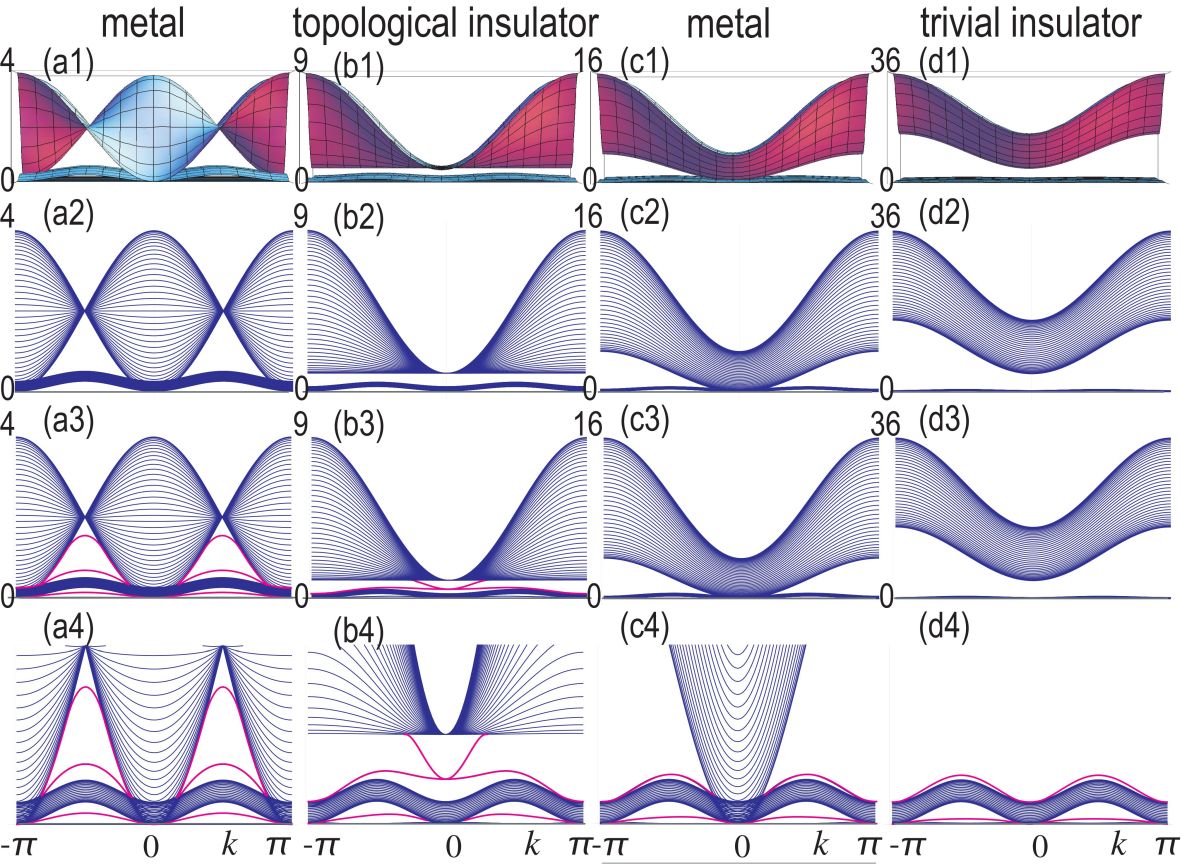
Figure 1: Band structures of a nanoribbon with 40-site width. The horizontal axis is the momentum $k$, and the vertical axis is the energy in unit of $t$. (a) Metal phase with $\mu=0$, (b) topological insulator phase with $\mu=t$, (c) metal phase with $\mu=2t$, and (d) trivial insulator phase with $\mu=4t$. We have set $\lambda=t$. (*1) Bird’s eye view of the bulk band. (*2) Projection of the bulk bands. (*3) Band structure of a nanoribbon. The edge states are marked in red. (*4) Enlarged band structure of (*3) near the zero energy. We have set $c_{3}=1$ and $c_{1}=0.25.$

In this work, for definiteness, we study such an explicit model that

$$m_{1} =t\left(\cos k_{x}+\cos k_{y}\right)-\mu,$$

$$m_{2} =\lambda\sin k_{x},\quad m_{3}=\lambda\sin k_{y}.$$ (11)

The band gap is calculated from (10) as

$$\Delta=\text{min}\left[\left|\pm 2t-\mu\right|,\left|\mu\right|\right]$$ (12)

at $\left(k_{x},k_{y}\right)=\left(0,0\right)$, $\left(0,\pi\right)$, $\left(\pi,0\right)$ or $\left(\pi,\pi\right)$. The band closes at $\mu=\pm 2t$ as in Fig.1.

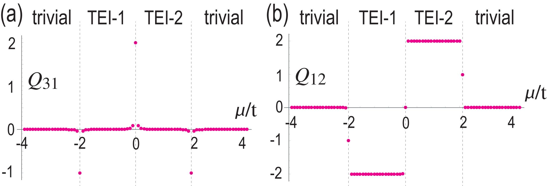
Figure 2: Euler number as a function of $\mu/t$ for (a) $Q_{31}$ and (b) $Q_{12}$. We note that $Q_{23}=0$ for all $\mu$. There are two topological-Euler-insulator phases denoted by TEI-1 and TEI-2. The horizontal axis is $\mu/t$.

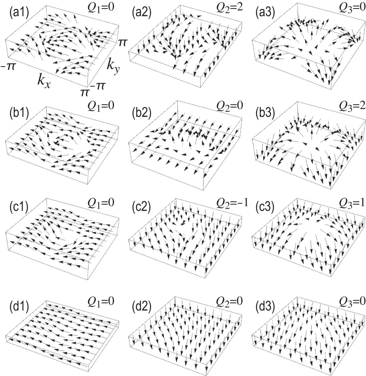
Figure 3: Spin textures in the $k_{x}$-$k_{y}$ plane for (*1) $\boldsymbol{n}_{1}$, (*2) $\boldsymbol{n}_{2}$ and (*3) $\boldsymbol{n}_{3}$, yielding the Pontryagin numbers $Q_{1}$, $Q_{2}$ and $Q_{3}$. (a*) Metal phase with $\mu=0$, (b*) topological insulator phase with $\mu=t$, (c*) metal phase with $\mu=2t$, and (d*) trivial insulator phase with $\mu=4t$. The corresponding Euler numbers are shown in Fig.2.

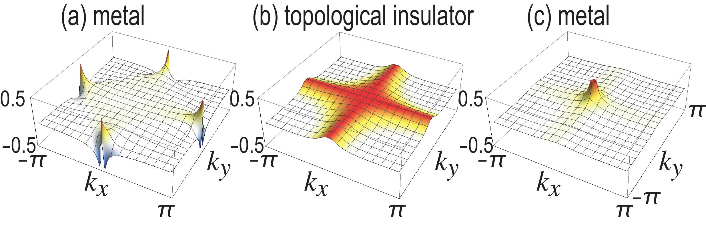
Figure 4: Local Pontraygin density in the $k_{x}$-$k_{y}$ plane for (a) metal phase with $\mu=0$, (b) topological insulator phase with $\mu=t$, and (c) metal phase with $\mu=2t$.

Topological number: We study the Euler number (4) or equivalently the Pontryagin number (5). They are related as $Q_{23}=Q_{1}$, $Q_{31}=Q_{2}$ and $Q_{12}=Q_{3}$. We have numerically integrated the Pontryagin density, whose results are shown in Fig.2. The Pontryagin number is graphically understood by plotting the direction of the vectors $\boldsymbol{n}_{i}$, as shown in Fig.3. It is nonzero only when the texture forms a skyrmion. It may change its value when the bulk band gap closes. It indicates that our system is a kind of topological insulators, which we call topological Euler insulators.

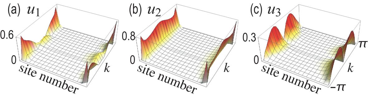
Figure 5: Absolute value of the eigenfunction for localized edge states in a nanoribbon with 40-site width. (a), (b) and (c) are for the bands $|u_{1}\rangle$, $|u_{2}\rangle$ and $|u_{3}\rangle$. They are well localized at the edges.

The Pontryagin number reads as follows. First we find $Q_{1}=0$. It is understood by the fact that the configuration (7) is restricted within the $yz$ plane. Next, we find $Q_{2}=2$ for $\mu=0$ and $Q_{2}=-1$ for $\mu=\pm t$, and $Q_{2}=0$ otherwise, as shown in Fig.2(a).

Finally, we find $Q_{3}=2$ for $0<\mu<2t$, $Q_{3}=-2$ for $-2t<\mu<0$, $Q_{3}=\pm 1$ for $\mu=\pm 2t$, and $Q_{3}=0$ otherwise, as shown in Fig.2(b). The local Pontryagin density $Q_{3}\left(k_{x},k_{y}\right)\equiv\boldsymbol{n}_{3}\cdot\left(\partial_{k_{x}}\boldsymbol{n}_{3}\times\partial_{k_{y}}\boldsymbol{n}_{3}\right)$ is given in Fig.4. It is interesting to note that the same topological phase diagram is produced by the following two-band model,

$$H_{2\text{band}}=\sum_{j=1,2,3}m_{j}\sigma_{j},$$ (13)

where $m_{j}$ are given by (11) and $\sigma_{j}$ are the Pauli matrices. This describes a Chern insulator for $0<\left|\mu\right|<2t$.

In conclusion, the system is topological for $0<\left|\mu\right|<2t$. The corresponding edge states emerge in the topological phase, as we now see.

Bulk-edge correspondence: We show the band structures of a nanoribbon in Fig.1. They coincide with those of bulk Hamiltonian except for the edge states marked in magenta. The eigenfunction is well localized at the edges as shown in Fig.5.

It is possible to study the edge states analytically. First, we study them at $k_{y}=\pi$, where the eigenequation is obtained from Eq.(9) as

$$\mu\left(\begin{array}[]{ccc}0&i\lambda\partial_{x}&0\\ i\lambda\partial_{x}&\mu&0\\ 0&0&0\end{array}\right)\left(\begin{array}[]{c}\left|u_{1}\right\rangle\\ \left|u_{2}\right\rangle\\ \left|u_{3}\right\rangle\end{array}\right)=E\left(\begin{array}[]{c}\left|u_{1}\right\rangle\\ \left|u_{2}\right\rangle\\ \left|u_{3}\right\rangle\end{array}\right)$$ (14)

in the first order of $k_{x}$. We find $\left|u_{3}\right\rangle=0$, as agrees with the numerical result in Fig.5(c). By assuming exponentially damping eigenfunctions for $\left|u_{1}\right\rangle$ and $\left|u_{2}\right\rangle$,

$$\left|u_{1}\right\rangle=c_{a}e^{\kappa x},\qquad\left|u_{2}\right\rangle=\pm ic_{a}e^{\kappa x},$$ (15)

we obtain from Eq.(14) that $\pm\mu\lambda\kappa=E$ and $-\mu\lambda\kappa\pm\mu^{2}=\pm E$. We solve the energy $E$ and the penetration depth $\kappa$ as

$$E=\frac{\mu^{2}}{2},\quad\kappa=\pm\frac{\mu}{2\lambda},$$ (16)

where $\kappa=\pm\mu/2\lambda$ describe the edge states localized at the right edge and the left edge, respectively. They agree well with the numerical results in Fig.1(b4) at $k=\pi$.

Next we study the edge states at $k_{y}=0$, where we have

$$\left(2t-\mu\right)\left(\begin{array}[]{ccc}0&-i\lambda\partial_{x}&0\\ -i\lambda\partial_{x}&2t-\mu&0\\ 0&0&0\end{array}\right)\left(\begin{array}[]{c}\left|u_{1}\right\rangle\\ \left|u_{2}\right\rangle\\ \left|u_{3}\right\rangle\end{array}\right)=E\left(\begin{array}[]{c}\left|u_{1}\right\rangle\\ \left|u_{2}\right\rangle\\ \left|u_{3}\right\rangle\end{array}\right)$$ (17)

in the first order of $k_{x}$. We have $\left|u_{3}\right\rangle=0$, as agrees with the numerical result in Fig.5(c). We have solutions

$$E=\frac{\left(2t-\mu\right)^{2}}{2},\quad\kappa=\mp\frac{2t-\mu}{2\lambda}.$$ (18)

These solutions show localized edge states at nonzero energies. They agree well with the numerical results in Fig.1(b4) at $k=0$.

Electric-circuit simulations: Electric circuits are characterized by the Kirchhoff current law. By making the Fourier transformation with respect to time, the Kirchhoff current law is expressed as

$$I_{a}\left(\omega\right)=\sum_{b}J_{ab}\left(\omega\right)V_{b}\left(\omega\right),$$ (19)

where $I_{a}$ is the current between node $a$ and the ground, while $V_{b}$ is the voltage at node $b$. The matrix $J_{ab}\left(\omega\right)$ is called the circuit Laplacian. Once the circuit Laplacian is given, we can uniquely setup the corresponding electric circuit. By equating it with the Hamiltonian $H$ asTECNature ; ComPhys

$$J_{ab}\left(\omega\right)=i\omega H_{ab}\left(\omega\right),$$ (20)

it is possible to simulate various topological phases of the Hamiltonian by electric circuitsTECNature ; ComPhys ; Hel ; Lu ; Research ; Zhao ; YLi ; EzawaTEC ; EzawaLCR ; EzawaSkin ; Garcia ; Hofmann ; EzawaMajo ; Tjunc ; Lee . The relations between the parameters in the Hamiltonian and in the electric circuit are determined by this formula.

In order to derive the circuit Laplacian, we explicitly write down the components of the Hamiltonian (9),

$$H_{11}= c_{3}[\frac{t^{2}}{2}\left(\cos 2k_{x}+\cos 2k_{y}+4\cos k_{x}\cos k_{y}+2\right)$$

$$-2\mu t\left(\cos k_{x}+\cos k_{y}\right)+\mu^{2}],$$ (21)

$$H_{22}= \frac{\lambda^{2}}{2}[c_{3}\left(1-\cos 2k_{x}\right)+c_{1}\left(1-\cos 2k_{y}\right)],$$ (22)

$$H_{33}= \frac{\lambda^{2}}{2}[c_{1}\left(1-\cos 2k_{y}\right)+c_{3}\left(1-\cos 2k_{y}\right)],$$ (23)

and

$$H_{12} =c_{3}[t\lambda\sin k_{x}\left(\cos k_{x}+\cos k_{y}\right)-\mu\lambda\sin k_{x}],$$ (24)

$$H_{13} =c_{3}[t\lambda\sin k_{y}\left(\cos k_{x}+\cos k_{y}\right)-\mu\lambda\sin k_{y}].$$ (25)

$$H_{23} =\left(c_{3}-c_{1}\right)\lambda^{2}\sin k_{x}\sin k_{y}.$$ (26)

Here, we make a convention that $t$, $\mu$ and $\lambda$ are dimensionless, and hence that $c_{1}$ and $c_{2}$ have the dimension of energy.

The circuit Laplacian is constructed as follows. To simulate the positive and negative hoppings in the Hamiltonian, we replace them with the capacitance $i\omega C$ and the inductance $1/i\omega L$, respectively. We note that $\sin k=(e^{ik}-e^{-ik})/2i$ represents an imaginary hopping in the tight-bind model. The imaginary hopping is realized by an operational amplifierHofmann .

We thus make the following replacements with respect to hoppings in the Hamiltonian to derive the circuit Laplacian: (i) $+X\rightarrow i\omega C_{X}$ for $X=t^{2},\mu^{2},\lambda^{2}$, where $C_{X}$ represents the capacitance whose value is $X$ [pF]. (ii) $-X\rightarrow 1/i\omega L_{X}$ for $X=\mu t,\lambda^{2}$, where $L_{X}$ represents the inductance whose value is $X$ [$\mu$H]. (iii) $\pm iX\rightarrow\pm 1/R_{X}$ for $X=t\lambda,\mu\lambda$, where $R_{X}$ represents the resistance whose value is $X$ [k$\Omega$].

Consequently, we obtain

$$J_{11}= \frac{i\omega c_{3}C_{t^{2}}}{2}\left(\cos 2k_{x}+\cos 2k_{y}+4\cos k_{x}\cos k_{y}+2\right)$$

$$+2\frac{1}{i\omega L_{\mu t}}\left(\cos k_{x}+\cos k_{y}\right)+i\omega C_{\mu^{2}},$$ (27)

$$J_{22}= \frac{c_{3}}{2}\left(i\omega C_{\lambda^{2}}+\frac{1}{i\omega L_{\lambda^{2}}}\cos 2k_{x}\right)$$

$$+\frac{c_{1}}{2}\left(i\omega C_{\lambda^{2}}+\frac{1}{i\omega L_{\lambda^{2}}}\cos 2k_{y}\right),$$ (28)

$$J_{33}= \frac{c_{1}}{2}\left(i\omega C_{\lambda^{2}}+\frac{1}{i\omega L_{\lambda^{2}}}\cos 2k_{x}\right)$$

$$+\frac{c_{3}}{2}\left(i\omega C_{\lambda^{2}}+\frac{1}{i\omega L_{\lambda^{2}}}\cos 2k_{y}\right),$$ (29)

and

$$J_{12} =\frac{c_{3}}{iR_{t\lambda}}\sin k_{x}\left(\cos k_{x}+\cos k_{y}\right)-\frac{c_{3}}{R_{\lambda\mu}}\sin k_{x},$$ (30)

$$J_{13} =\frac{c_{3}}{iR_{t\lambda}}\sin k_{x}\left(\cos k_{x}+\cos k_{y}\right)-\frac{c_{3}}{R_{\lambda\mu}}\sin k_{x},$$ (31)

$$J_{23} =i\omega\left(c_{3}-c_{1}\right)C_{\lambda^{2}}\sin k_{x}\sin k_{y}.$$ (32)

Furthermore, in order to realize impedance resonances, we add a circuit corresponding toTECNature ; ComPhys ; EzawaTEC ; EzawaMajo ; Tjunc

$$\Delta J_{11}=\Delta J_{22}=\Delta J_{33}=i\omega C_{0}+\frac{1}{i\omega L_{0}},$$ (33)

which vanish at the critical frequency $\omega_{0}=1/\sqrt{L_{0}C_{0}}$.

After the diagonalization, the circuit Laplacian yields

$$J_{n}\left(\omega\right)=i\omega C_{0}+\frac{1}{i\omega L_{0}}-i\omega\varepsilon_{n}\left(\omega\right),$$ (34)

where $\varepsilon_{n}$ is the eigenvalue of the circuit Laplacian. Solving $J_{n}\left(\omega\right)=0$, we obtain

$$\omega_{\text{R}}(\varepsilon_{n})=\sqrt{L_{0}/(C_{0}-\varepsilon_{n})},$$ (35)

which corresponds to the impedance resonance frequency.

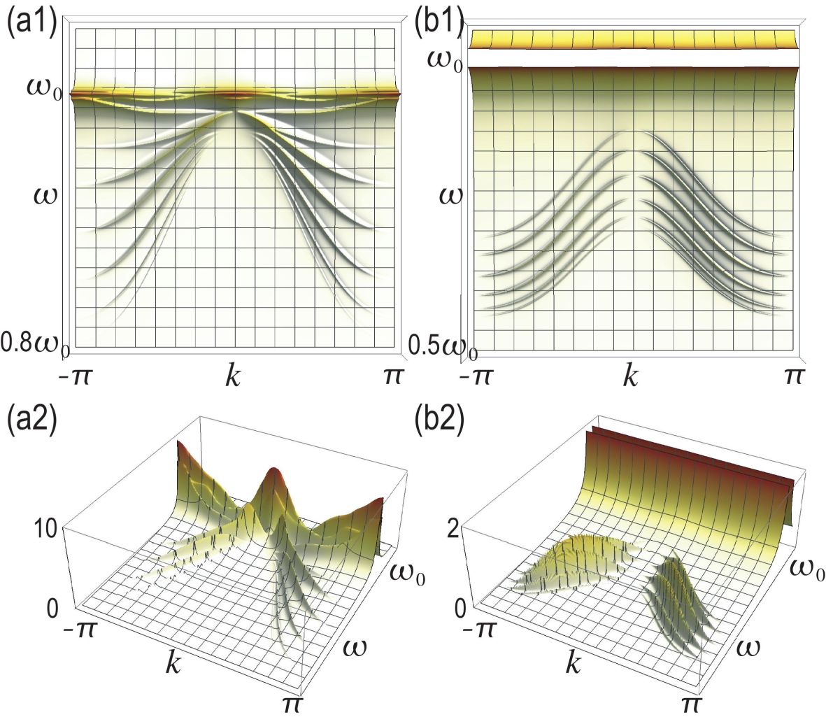
Figure 6: Impedance in the $k$-$\omega$ plane. (a*) Topological phase with $\mu=-t$ and (b*) trivial phase with $\mu=-4t$. (*1) Top view and (*2) bird’s eye’s view. We have set $c_{3}=1$ and $c_{1}=0.25$. The vertical axis is the impedance in unit of k$\Omega$.

Topological edge states are observed by impedance resonances, where the impedance between nodes $a$ and $b$ is given byHel $Z_{ab}\equiv V_{a}/I_{a}=G_{ab}$, where $G$ is the Green function defined by the inverse of the circuit Laplacian $J$, $G\equiv J^{-1}$. The momentum-dependent impedance is an experimentally detectable quantityHel ; Lee by using a Fourier transformation along the nanoribbon direction $y$,

$$Z_{\alpha\beta}\left(x,k_{y},\omega\right)=\sum_{\rho}Z_{\alpha\beta}\left(x_{\rho},y_{\rho},\omega\right)\exp\left[-iy_{\rho}k_{y}\right],$$ (36)

where $\left(x_{\rho},y_{\rho}\right)$ is the Bravais vector. We take $\alpha=\beta$ at edge sites.

We show an impedance as a function of the momentum $k$ and the frequency $\omega$ in Fig.6. Topological edge states are clearly observed in the topological phase. Note that the top and the bottom are reversed between the band structure and the impedance resonance, as indicated in Eq.(35), where $\varepsilon_{n}$ represents the band structure while $\omega_{\text{R}}$ the impedance resonance.

In this work we have proposed topological Euler insulators, which are characterized by nontrivial Euler numbers. Their band structure including the edge states is well observed by measuring the impedance of the corresponding electric circuit.

The author is very much grateful to N. Nagaosa for helpful discussions on the subject. This work is supported by the Grants-in-Aid for Scientific Research from MEXT KAKENHI (Grants No. JP17K05490 and No. JP18H03676). This work is also supported by CREST, JST (JPMJCR16F1 and JPMJCR20T2).

References

(1) M. Z. Hasan and C. L. Kane, Rev. Mod. Phys. 82,
3045 (2010).
(3) J. Ahn, S. Park and B. J. Yang, Phys. Rev. X 9, 021013 (2019).
(4) A. Bouhon, Q. Wu, R.-J. Slager, H. Weng, O. V. Yazyev and
T. Bzdusek, Nature Physics (2020).
(5) F. Nur Unal, A. Bouhon and R.-J. Slager, Phys. Rev. Lett.
125, 053601 (2020).
(6) S. Imhof, C. Berger, F. Bayer, J. Brehm, L. Molenkamp,
T. Kiessling, F. Schindler, C. H. Lee, M. Greiter, T. Neupert, R. Thomale,
Nat. Phys. 14, 925 (2018).
(7) C. H. Lee , S. Imhof, C. Berger, F. Bayer, J. Brehm, L. W.
Molenkamp, T. Kiessling and R. Thomale, Communications Physics, 1,
39 (2018).
(8) T. Helbig, T. Hofmann, C. H. Lee, R. Thomale, S. Imhof, L. W.
Molenkamp and T. Kiessling, Phys. Rev. B 99, 161114 (2019).
(9) Y. Lu, N. Jia, L. Su, C. Owens, G. Juzeliunas, D. I. Schuster
and J. Simon, Phys. Rev. B 99, 020302 (2019).
(10) K. Luo, R. Yu and H. Weng, Research (2018), ID 6793752.
(11) E. Zhao, Ann. Phys. 399, 289 (2018).
(12) Y. Li, Y. Sun, W. Zhu, Z. Guo, J. Jiang, T. Kariyado, H. Chen
and X. Hu, Nat. Com. 9, 4598 (2018).
(13) M. Ezawa, Phys. Rev. B 98, 201402(R) (2018).
(14) M. Serra-Garcia, R. Susstrunk and S. D. Huber, Phys. Rev. B
99, 020304 (2019).
(15) T. Hofmann, T. Helbig, C. H. Lee, M. Greiter, R. Thomale,
Phys. Rev. Lett. 122, 247702 (2019).
(16) M. Ezawa, Phys. Rev. B 100, 045407 (2019)
(17) M. Ezawa, Phys. Rev. B 99, 201411(R) (2019).
(18) M. Ezawa, Phys. Rev. B 99, 121411(R) (2019).
(19) M. Ezawa, Phys. Rev. B 102, 075424 (2020).
(20) C. H. Lee, T. Hofmann, T. Helbig, Y. Liu, X. Zhang, M. Greiter
and R. Thomale, Nature Communications, 11, 4385 (2020).