The $\mathcal{F}$-family of covariance functions: A Matérn analogue for modeling random fields on spheres

Abstract

The Matérn family of isotropic covariance functions has been central to the theoretical development and application of statistical models for geospatial data. For global data defined over the whole sphere representing planet Earth, the natural distance between any two locations is the great circle distance. In this setting, the Matérn family of covariance functions has a restriction on the smoothness parameter, making it an unappealing choice to model smooth data. Finding a suitable analogue for modelling data on the sphere is still an open problem. This paper proposes a new family of isotropic covariance functions for random fields defined over the sphere. The proposed family has a parameter that indexes the mean square differentiability of the corresponding Gaussian field, and allows for any admissible range of fractal dimension. Our simulation study mimics the fixed domain asymptotic setting, which is the most natural regime for sampling on a closed and bounded set. As expected, our results support the analogous results (under the same asymptotic scheme) for planar processes that not all parameters can be estimated consistently. We apply the proposed model to a dataset of precipitable water content over a large portion of the Earth, and show that the model gives more precise predictions of the underlying process at unsampled locations than does the Matérn model using chordal distances.

Keywords:

Great circle distance, Fractal dimension, Matérn covariance function, Mean square differentiability

1 Introduction

1.1 Context

The last decades have seen an unprecedented increase in the availability of georeferenced datasets of global extent, for example in the form of environmental monitoring networks or climate model ensembles (Castruccio and Stein, 2013; Porcu et al., 2018). This increase in data-availability has in turn motivated the mathematical and statistical communities to develop models for random fields defined on the two-dimensional surface of the sphere, representing our planet.

The Gaussian assumption implies that the finite dimensional distributions are completely specified through the mean and covariance function. Covariance functions are positive definite, and proving such a requirement involves substantial theoretical work. We refer the reader to Schoenberg (1942); Gneiting (2013); Porcu et al. (2016); Berg and Porcu (2017) and White and Porcu (2018) for the established theory about positive definite functions on the $d$-dimensional sphere of $\mathbb{R}^{d+1}$, for $d$ being a positive integer. Also, comprehensive recent reviews can be found in Jeong et al. (2018) and in Porcu et al. (2018).

In spatial statistics, it is very common to assume the covariance function of a random field $Z$ to be isotropic, that is the covariance between $Z(\bm{x}_{1})$ and $Z(\bm{x}_{2})$ depends only on the distance between $\bm{x}_{1}$ and $\bm{x}_{2}$. For global data, the natural metric is the geodesic or great circle distance, defined as the length of the shortest arc joining two points located over the spherical shell.

The Matérn covariance function is widely considered as the default choice for modelling spatial variation (Stein, 1999). Its main attractive feature is its inclusion of a parameter that allows the user to control the fractal dimension and the mean square differentiability of the associated Gaussian process. In turn, this has been shown to be a fundamental aspect in evaluating predictive performance of covariance functions under infill asymptotics (Zhang, 2004). The Matérn covariance has also a nice closed form expression for the associated spectral density, which is convenient for theoretical analysis of the properties of maximum likelihood (ML) estimators (Zhang, 2004), approximate likelihood (Furrer et al., 2006; Bevilacqua et al., 2012; Kaufman and Shaby, 2013) and misspecified linear unbiased prediction (Stein, 1999) under infill asymptotics. A wealth of results is also available within SPDE’s with Gaussian Markov approximations (Lindgren et al., 2011) as well as in the numerical analysis literature. We refer the reader to Scheuerer et al. (2013) for more details.

1.2 The problem

Gneiting (2013) shows that Matérn covariance functions are no longer positive definite on the sphere when coupled with the geodesic distance, unless a severe restriction is imposed on the smoothing parameter. Essentially, the Matérn covariance function can be used only for very rough realisations of the associated Gaussian process. Alternatively, the Matérn model can be adapted to the sphere by using the chordal distance, but such a choice would be suboptimal and we refer the reader to Banerjee (2005); Gneiting (2013); Jeong and Jun (2015b); Porcu et al. (2016) for constructive criticism about the use of the chordal distance.

The problem of obtaining a spherical analogue of the Matérn function that allows different degrees of differentiability has been addressed by using smoothing techniques of non-differentiable random fields (Jeong and Jun, 2015a) and by modelling the spectral representation of the covariance function on the sphere (Guinness and Fuentes, 2016), providing the so-called circular Matérn model. The first approach does not allow for closed form expressions, whilst the second approach allows the use of linear combinations of hypergeometric polynomials to obtain closed form expressions, and of its series expansion for computations. Even though both approaches allow to index mean square differentiability, the lack of software makes the implementation difficult. Further, the computational problem increases when the smoothness of the covariance function at the origin decreases, as the convergence of the series becomes extremely slow. As a result, finding the analogue of the Matérn covariance function on the sphere is a challenging problem. In conclusion, the search for covariance functions on spheres that allow for a continuous parameterisation of smoothness is still elusive, and has been explicitly stated as an open problem in two collections of challenges posed by Gneiting (2013) and Porcu et al. (2018). Here we provide a solution to this problem.

1.3 Our contribution

We propose a class of covariance functions for $d$-dimensional spheres, that we term ${\cal F}$ class, having the same properties as the Matérn covariance function on planar surfaces. Specifically, the new class is specified through the Gauss hypergeometric function, which has been widely studied in the numerical analysis literature (see Johansson, 2017, and references therein). For computation, we use the C library GSL (Galassi et al., 1996). However, libraries such as ARB (Johansson, 2017) can be used as well.

We show that the new class has a parameter that allows for a continuous parameterisation of smoothness at the origin. Further, the same parameter allows for indexing fractal dimension of random surfaces on circles or spheres. Finally, we prove this class to admit several interesting closed form expressions that can be easily coded. Most applications deal with the two dimensional sphere, but for mathematical completeness we present our results over the $d$-dimensional sphere.

The plan of the paper is the following. Section 2 contains preliminaries needed for the subsequent presentation. Section 3 introduces the ${\cal F}$-Family of covariance functions on spheres. We then study mean square differentiability and fractal dimension properties of Gaussian fields on spheres with the new class of covariance functions. Section 4 describes a simulation study to understand how well the parameters of the new covariance function can be estimated through ML. Our simulation study mimics the infill (or fixed domain) asymptotic framework (Stein, 1999) that is relevant for processes defined over closed and bounded sets. We especially focus on the estimation of scale, variance, and microergodic parameter (Stein, 1999) when the smoothing parameter is fixed. Our simulations suggest that consistent estimation of the scale and variance parameters is not achieveable, but that the microergodic parameter can be estimated consistently. Section 5 analyses a dataset corresponding to monthly averages of precipitable water content over a large portion of the planet Earth with a spatial resolution of $2.5$ degrees across longitudes and latitudes, available at https://www.esrl.noaa.gov/psd/ (See Kalnay et al., 1996). We show that the new class of covariance functions delivers better predictive performance on this dataset than both the Matérn covariance function based on chordal distance and the circular Matérn covariance function. The paper concludes with discussion. Technical details and generalisations that might be useful for future research are given in Appendices A and B respectively. The codes associated with Sections 4 and 5 are available at the following GitHub repository: https:$//$github.com$/$FcoCuevas87$/{\text{F}}\_{}{\text{F}}$amil${\text{y}}\_{}{\text{c}}$ova.

2 Background

2.1 Covariance functions and distances

This section provides a background on random fields on the sphere, their covariance functions and their spectral representation. For a positive integer $d$, $\mathbb{S}^{d}=\{\bm{x}\in\mathbb{R}^{d+1},\|\bm{x}\|=1\}$ denotes the surface of the $d$-dimensional unit sphere embedded in $\mathbb{R}^{d+1}$, with $\|\cdot\|$ denoting Euclidean norm. We shall sometimes refer to the Hilbert sphere $\mathbb{S}^{\infty}=\{\bm{x}\in\mathbb{R}^{\mathbb{N}},\|\bm{x}\|=1\}$. The natural metric on $\mathbb{S}^{d}$ is the great circle distance,

$$\theta(\bm{x}_{1},\bm{x}_{2})=\arccos(\bm{x}_{1}^{\top}\bm{x}_{2})\in[0,\pi],$$

for $\bm{x}_{1},\bm{x}_{2}\in\mathbb{S}^{d}$, where $\top$ denotes transpose. The chordal distance on $\mathbb{S}^{d}$ is

$$d_{{\rm CH}}(\bm{x}_{1},\bm{x}_{2})=\|\bm{x}_{1}-\bm{x}_{2}\|=2\sin\left(\frac{\theta(\bm{x}_{1},\bm{x}_{2})}{2}\right),\qquad\bm{x}_{1},\bm{x}_{2}\in\mathbb{S}^{d}.$$ (1)

We denote by $Z=\{Z(\bm{x}),\bm{x}\in\mathbb{S}^{d}\}$ a random field on $\mathbb{S}^{d}$, with constant mean and covariance function $C(\bm{x}_{1},\bm{x}_{2})={\rm cov}\{Z(\bm{x}_{1}),Z(\bm{x}_{2})\}$, for $\bm{x}_{1},\bm{x}_{2}\in\mathbb{S}^{d}$. The requirement for validity of a candidate function $C(\bm{x}_{1},\bm{x}_{2})$ to be a covariance function is that for any positive integer $n$, locations $\bm{x}_{1},\ldots,\bm{x}_{n}\in\mathbb{S}^{d}$ and real numbers $c_{1},\ldots,c_{n}$,

$${\rm Var}\left(\sum_{i=1}^{n}c_{i}Z(\bm{x}_{i})\right)=\sum_{i,j=1}^{n}c_{i}c_{j}C(\bm{x}_{i},\bm{x}_{j})\geq 0.$$ (2)

Mappings $C$ that satisfy Equation (2) are called positive definite, or strictly positive definite if the inequality is strict for any non-zero collection of real numbers $c_{1},\ldots,c_{n}$ and distinct locations $\bm{x}_{1},\ldots,\bm{x}_{n}$.

If in addition

$$C(\bm{x}_{1},\bm{x}_{2})=\sigma^{2}\psi(\theta(\bm{x}_{1},\bm{x}_{2})),\qquad\bm{x}_{1},\bm{x}_{2}\in\mathbb{S}^{d},$$ (3)

for some value $\sigma^{2}>0$ and mapping $\psi:[0,\pi]\rightarrow\mathbb{R}$ such that $\psi(0)=1$, then $C$ is called a geodesically isotropic covariance (Porcu et al., 2018), and $\sigma^{2}$ is the variance of $Z$. Throughout, we use $\theta$ to denote great circle distance whenever no confusion can arise. Also, we shall not distinguish between positive and strict positive definiteness unless specifically required. We define $\Psi_{d}$ as the class of continuous functions $\psi$ associated with the covariance function $C$ on $\mathbb{S}^{d}$ through the identity (3). We also define $\Psi_{\infty}=\bigcap_{d=1}^{\infty}\Psi_{d}$, with the strict inclusion relation

$$\Psi_{1}\supset\Psi_{2}\supset\cdots\supset\Psi_{d}\supset\cdots\supset\Psi_{\infty},$$

proved by Gneiting (2013).

2.2 Spectral Theory

Spectral representations for positive definite functions on spheres are equivalent to Bochner and Schoenberg’s theorems in Euclidean spaces (see Daley and Porcu, 2013, and references therein). Schoenberg (1942) showed that a continuous mapping $\psi:[0,\pi]\rightarrow\mathbb{R}$ belongs to the class $\Psi_{d}$ if and only if it can be uniquely written as

$$\psi(\theta)=\sum_{n=0}^{\infty}b_{n,d}\frac{P_{n}^{(d-1)/2}(\cos\theta)}{P_{n}^{(d-1)/2}(1)},\qquad\theta\in[0,\pi],$$ (4)

where $P_{n}^{\lambda}$ denotes the $\lambda$-Gegenbauer polynomial of degree $n$ (Abramowitz and Stegun, 1965, 22.2.3), and $\{b_{n,d}\}_{n=0}^{\infty}$ is a probability mass function.

Schoenberg (1942) also showed that $\psi$ belongs to the class $\Psi_{\infty}$ if and only if

$$\psi(\theta)=\sum_{n=0}^{\infty}b_{n}(\cos\theta)^{n},\qquad\theta\in[0,\pi],$$ (5)

with $\{b_{n}\}_{n=0}^{\infty}$ being again a probability mass function. We follow Daley and Porcu (2013) in calling the sequence $\{b_{n,d}\}_{n=0}^{\infty}$ in (4) a $d$-Schoenberg sequence, to emphasise the dependence on the index $d$ in the class $\Psi_{d}$. Analogously, we call $\{b_{n}\}_{n=0}^{\infty}$ a Schoenberg sequence. Fourier inversion allows for an explicit representation of the sequences $\{b_{n,d}\}_{n=0}^{\infty}$. Specifically, for $d=1$ we have that (see Gneiting, 2013)

$$b_{0,1}=\int_{0}^{\pi}\psi(\theta){\rm d}\theta\qquad\mbox{ and }\qquad b_{n,1}=\frac{2}{\pi}\int_{0}^{\pi}\cos(n\theta)\psi(\theta){\rm d}\theta,\mbox{ for }n\geq 1,$$ (6)

whereas for $d\geq 2$ we have

$$b_{n,d}=\kappa(n,d)\int_{0}^{\pi}\psi(\theta)P_{n}^{(d-1)/2}(\cos\theta)\left(\sin\theta\right)^{d-1}{\rm d}\theta,$$ (7)

where $\kappa(n,d)$ is a positive constant (see Gneiting, 2013).

Lang and Schwab (2013) showed that the rate of decay of the $d$-Schoenberg sequence determines the regularity properties of the associated Gaussian field in terms of interpolation spaces and Hölder continuities of the sample paths. The $d$-Schoenberg sequences are useful in contexts as diverse as spatial statistics (Guinness and Fuentes, 2016), equivalence of Gaussian measures and infill asymptotics (Arafat et al., 2018), approximation theory (Menegatto et al., 2006; Beatson et al., 2014; Ziegel, 2014; Massa et al., 2017) and spatial point processes (Møller et al., 2018). In practice, the $d$-Schoenberg sequence of a parametric model is rarely known and it must be computed via numerical integration.

To build parametric models, it is common to use Equation (5) and the relationship between probability mass functions and the associated probability generating functions. This procedure yields covariance functions models with known Schoenberg sequences. Table 1 in Gneiting (2013) provides a list of parametric models where the Schoenberg sequence is known (see also Soubeyrand et al., 2008; Porcu et al., 2016).

The Negative Binomial probability distribution is defined through the coefficients

$$b_{n}(\delta,\tau)=\binom{n+\tau-1}{n}\delta^{n}(1-\delta)^{\tau},\qquad\delta\in(0,1),\tau>0,\quad n=0,1,\ldots.$$ (8)

Using the coefficients $b_{n}(\delta,\tau)$ in concert with the expansion (5), Gneiting (2013) obtains the Negative Binomial family of members of the class $\Psi_{\infty}$, denoted ${\cal N}_{\delta,\tau}$ throughout, and defined as

$${\cal N}_{\delta,\tau}(\theta)=\left(\frac{1-\delta}{1-\delta\cos\theta}\right)^{\tau},\qquad\theta\in[0,\pi].$$ (9)

One limitation of the Negative Binomial family is that its elements are infinitely differentiable at the origin, making them not very appealing for spatial interpolation (Stein, 1999). Nevertheless, we shall use the function ${\cal N}_{\delta,\tau}$ as the starting point for the construction of our proposed family.

2.3 The Matérn and the circular Matérn classes

The Matérn class of covariance functions, ${\cal M}_{\nu,\alpha}$, is defined as (Stein, 1999)

$${\cal M}_{\nu,\alpha}(d_{{\rm CH}})=\frac{2^{1-\nu}}{\Gamma(\nu)}\left(\frac{d_{{\rm CH}}}{\alpha}\right)^{\nu}{\cal K}_{\nu}\left(\frac{d_{{\rm CH}}}{\alpha}\right),$$ (10)

where $d_{{\rm CH}}$ is the chordal distance as defined at (1), with $\alpha,\nu>0$ and ${\cal K}_{\nu}$ a modified Bessel function of the second kind of order $\nu$ (Abramowitz and Stegun, 1965, 9.6.22). The importance of the Matérn class stems from the parameter $\nu$ that controls the differentiability (in the mean square sense) of the associated Gaussian field. Specifically, for any positive integer $k$, a Gaussian field with Matérn covariance function is $k$-times mean square differentiable if and only if $\nu>k$. Also, the Matérn function converges to the Gaussian kernel as $\nu\rightarrow\infty$. When $\nu=k+1/2$, for $k$ a positive integer, the Matérn covariance function simplifies into the product of an exponential covariance with a polynomial of order $k$. For instance, ${\cal M}_{1/2,1}(d_{{\rm CH}})=\exp(-d_{{\rm CH}})$ and ${\cal M}_{3/2,1}(d_{{\rm CH}})=\exp(-d_{{\rm CH}})(1+d_{{\rm CH}})$. Observe that ${\cal M}_{\nu,\alpha}(0)=1$, so that ${\cal M}_{\nu,\alpha}$ is actually a correlation function, and must be premultiplied by a variance parameter to obtain a covariance function.

The Matérn covariance function is not in general a valid covariance function on ${\mathbb{S}}^{2}$. Lemma 1 in Gneiting (2013) shows that the function $\theta\mapsto{\cal M}_{\nu,\alpha}(\theta)$, $\theta\in[0,\pi]$, is not a member of the class $\Psi_{1}$ if $\nu>1/2$. Thus, the Matérn class cannot be used to index arbitrary degrees of differentiability on spheres if coupled with the great circle distance.

Guinness and Fuentes (2016) have proposed the circular Matérn covariance function, ${\cal C}_{\nu,\alpha}$, given by

$${\cal C}_{\nu,\alpha}(\theta)=\frac{1}{S(\alpha,\nu)}\sum_{n=0}^{\infty}\frac{1}{(n^{2}+\alpha^{2})^{\nu+1/2}}\cos(n\theta),\quad\theta\in[0,\pi],$$ (11)

with $S(\alpha,\nu)=\sum_{n=0}^{\infty}(n^{2}+\alpha^{2})^{-(\nu+1/2)}$.

Arguments in Gneiting (2013) show that ${\cal C}_{\nu,\alpha}$ belongs to the class $\Phi_{3}$. This model is an adaptation of the classical spectral representation of the Matérn covariance on Euclidean spaces to the spherical case. Guinness and Fuentes (2016) show that the parameter $\nu$ controls the mean square differentiability of the associated Gaussian field on $\mathbb{S}^{2}$, and provide closed form expressions when $\nu$ is a half integer.

3 The ${\cal F}$-family of covariance functions

We now let

$${}_{2}F_{1}(a,b,c;z)=\sum_{n=0}^{\infty}\frac{(a)_{n}(b)_{n}}{(c)_{n}}\frac{z^{n}}{n!},\quad|z|<1,$$

denote the Gauss Hypergeometric function, where $(\cdot)_{n}$ denotes the Pochhammer symbol (Abramowitz and Stegun, 1965, 6.1.22) and complex numbers $a$, $b$, $c$. As detailed in Whittaker and Watson (1996, p. 282), for $c>0$, the Gauss hypergeometric function converges for all $|z|<1$, and converges absolutely for $|z|=1$ provided

$$\mathrm{Re}(c-a-b)>0,$$ (12)

where $\mathrm{Re}(x)$ denotes the real part of a complex number $x$. We now define the ${\cal F}={\cal F}_{\tau,\alpha,\nu}$ family of functions through the identity

$$\mathcal{F}_{\tau,\alpha,\nu}(\theta)=\frac{B(\alpha,\nu+\tau)}{B(\alpha,\nu)}{}_{2}F_{1}(\tau,\alpha,\alpha+\nu+\tau;\cos\theta),\qquad\theta\in[0,\pi],$$ (13)

where $B(\cdot,\cdot)$ denotes the Beta function (Abramowitz and Stegun, 1965, 6.2.1) and the parameters $\tau,\alpha$ and $\nu$ are strictly positive. We are now ready to illustrate the main result of this section.

Theorem 3.1.

Let $\tau$, $\alpha$ and $\nu$ be strictly positive. Then, the function ${\cal F}_{\tau,\alpha,\nu}$ defined through Equation (13) is a member of the class $\Psi_{\infty}$. Additionally, it can be written as a mixture of Negative Binomial covariance functions.

Proof. We give a constructive proof based on the following criterion that can be found in Lemma 1 in Gneiting (2013), adapted to our notation.

Lemma 3.2.

Let $q$ be a positive integer, $A\subseteq\mathbb{R}^{q}$ and let $\mu$ be a Borel probability measure on $A$. Let $\psi_{c}:[0,\pi]\to\mathbb{R}$ be an element of the class $\Psi_{\infty}$ for any $c\in A$. Then, the function $\psi:[0,\pi]\to\mathbb{R}$ defined by

$$\psi(\theta)=\int_{A}\psi_{c}(\theta)\mu({\rm d}c),\qquad\theta\in[0,\pi],$$ (14)

belongs to the class $\Psi_{\infty}$.

We now consider the Negative Binomial family ${\cal N}_{\delta,\tau}$ as defined in Equation (9), and the Beta probability measure

$$\mu_{\alpha,\nu}({\rm d}\delta)=\frac{1}{B(\alpha,\nu)}\delta^{\alpha-1}(1-\delta)^{\nu-1}{\rm d}\delta,\qquad\delta\in(0,1),\quad\alpha,\nu>0.$$ (15)

We invoke Lemma 3.2 to claim that $\mathcal{F}_{\tau,\alpha,\nu}\in\Psi_{\infty}$ because

$$\mathcal{F}_{\tau,\alpha,\nu}(\theta)=\int_{(0,1)}{\cal N}_{\delta,\tau}(\theta)\mu_{\alpha,\nu}({\rm d}\delta),\qquad\theta\in[0,\pi].$$ (16)

In fact, direct inspection shows that, for $\theta\in[0,\pi]$,

$$\frac{1}{B(\alpha,\nu)}\int_{0}^{1}\left(\frac{1-\delta}{1-\delta\cos\theta}\right)^{\tau}\delta^{\alpha-1}(1-\delta)^{\nu-1}\mathrm{d}\delta$$

$$= \frac{1}{B(\alpha,\nu)}\int_{0}^{1}\left(\sum_{n=0}^{\infty}\binom{n+\tau-1}{n}(1-\delta)^{\tau}\delta^{n}(\cos\theta)^{n}\right)\delta^{\alpha-1}(1-\delta)^{\nu-1}\mathrm{d}\delta$$

$$= \frac{B(\alpha,\nu+\tau)}{B(\alpha,\nu)}\sum_{n=0}^{\infty}\left(\int_{0}^{1}\delta^{n}\frac{\delta^{\alpha-1}(1-\delta)^{\tau+\nu-1}}{B(\alpha,\nu+\tau)}\mathrm{d}\delta\right)\frac{(\tau)_{n}}{n!}(\cos\theta)^{n},$$ (17)

where the second equality comes from (8), and the last equality comes from dominated convergence. Note that the integral of the last expression corresponds to the $n$-th moment of a Beta distribution with shape parameters $\alpha$ and $\tau+\nu$, which is given by $(\alpha)_{n}/(\alpha+\tau+\nu)_{n}$ (Johnson et al., 1995). Thus, it follows that

$$\sum_{n=0}^{\infty}\frac{(\alpha)_{n}(\tau)_{n}}{(\alpha+\nu+\tau)_{n}}\frac{(\cos\theta)^{n}}{n!} = {}_{2}F_{1}(\tau,\alpha,\alpha+\nu+\tau;\cos\theta),\qquad\theta\in[0,\pi],$$ (18)

which shows that (16) and (13) agree as asserted. The proof is completed by invoking Schoenberg (1942) theorem for the class $\Psi_{\infty}$, which is in turn described through our Equation (5). $\Box$

Notice that condition (12) is achieved since $\nu>0$. Also, ${\cal N}_{\delta,\tau}(0)=1$ implies that $\mathcal{F}_{\tau,\alpha,\nu}(0)=1$. This reproduces the result for $z=1$ (Olver et al., 2010, equation 15.4.20):

$${}_{2}F_{1}(\tau,\alpha,\alpha+\nu+\tau;1)=\frac{B(\alpha,\nu)}{B(\alpha,\nu+\tau)}=\frac{\Gamma(\nu)\Gamma(\alpha+\tau+\nu)}{\Gamma(\alpha+\nu)\Gamma(\tau+\nu)},$$ (19)

provided that $\alpha,\tau$ and $\nu$ are positive real numbers.

The proof of Theorem 3.1 shows that the $\mathcal{F}$ class is obtained from the probability generating function of the so called Beta-Negative Binomial distribution (Johnson et al., 2005). The Schoenberg coefficients associated with the ${\cal F}$ class are uniquely defined as

$$b_{n}(\tau,\alpha,\nu)=\frac{B(\alpha,\nu+\tau)}{B(\alpha,\nu)}\frac{(\alpha)_{n}(\tau)_{n}}{(\alpha+\nu+\tau)_{n}n!},\qquad n=0,1,\ldots.$$ (20)

The associated $d$-Schoenberg coefficients $b_{n,d}(\tau,\alpha,\nu)$ are computed using Theorem 4.2(b) from Møller et al. (2018) and are given in Appendix A. Moreover, as a consequence of Stirling’s formula, we derive

$$b_{n}(\tau,\alpha,\nu)\sim M(\alpha,\tau,\nu)n^{-(1+\nu)},\qquad n\to\infty,$$ (21)

where $M(\alpha,\tau,\nu)$ is a positive constant that depends on $\alpha,\tau$ and $\nu$. Here, for two functions $f,g:\mathbb{N}\to\mathbb{R}$, $f(n)\sim g(n)$ as $n\to\infty$ if and only if $\lim_{n\to\infty}f(n)/g(n)=1$.

Equation (21) shows how the parameter $\nu$ controls the rate of decay of the Schoenberg coefficients. This is connected with the mean square differentiability (Lang and Schwab, 2013) and the fractal dimension of the associated Gaussian random field (Hansen et al., 2015).

3.1 Mean square differentiability

Defining mean square differentiability for a stochastic process defined on $\mathbb{S}^{d}$ needs care, as derivatives are not taken along straight lines (as in the case of processes defined over Euclidean spaces). Guinness and Fuentes (2016) provide a definition based on great circles, whilst Lin et al. (2019) define mean square differentiability through directional derivatives on manifolds. Albeit working on slightly different frameworks, the authors reach the same conclusion: for a Gaussian random field $Z$ that is isotropic on $\mathbb{S}^{d}$, with covariance function $C$ defined through Equation (3), for some member $\psi$ within the class $\Psi_{d}$, mean square differentiability of order $n$ of $Z$ is equivalent to the fact that the $2n$-th derivative of the even extensions of $\psi$ evaluated at zero, denoted $\psi^{(2n)}(0)$ throughout, exists and is finite.

Note that all the parametric families within the class $\Psi_{\infty}$ listed in Table 1 of Gneiting (2013) are either nondifferentiable (e.g., the Sine Power family, see also Soubeyrand et al., 2008) or infinitely differentiable at the origin (e.g., the Poisson and Negative Binomial families). Hence, the associated random fields are infinitely differentiable or nondifferentiable in the mean square sense.

The following result shows that the parameter $\nu$ controls the smoothness of a random field with covariance $\mathcal{F}_{\tau,\alpha,\nu}(\theta)$. In what follows, $\lfloor x\rfloor$ denotes the largest integer less than or equal to $x\in\mathbb{R}$.

Proposition 3.3.

Let $d$ and $n$ be positive integers. Let $Z$ be an isotropic Gaussian random field on $\mathbb{S}^{d}$ with covariance function given by $\mathcal{F}_{\tau,\alpha,\nu}(\theta)$ as in Equation (13). Then, $Z$ is $n$ times mean square differentiable if and only if $\lfloor\nu\rfloor>n$.

Proof. Our proof is based on direct application of Theorem 1 in Guinness and Fuentes (2016): let $Z$ be a Gaussian random field on $\mathbb{S}^{d}$ with isotropic covariance function $C$ defined through the family $\mathcal{F}_{\tau,\alpha,\nu}$ defined at (13). Then, $Z$ is $n$ times mean square differentiable if and only if $\mathcal{F}^{(2n)}_{\tau,\alpha,\nu}(0)$ (intended as even extension) exists and is finite. To simplify the calculations below, we write

$$f_{\delta,\tau}(\cos\theta)=(1-\delta)^{-\tau}{\cal N}_{\delta,\tau}(\theta)=(1-\delta\cos\theta)^{-\tau},$$

with ${\cal N}_{\delta,\tau}$ being the Negative Binomial family in Equation (9). Using this change of notation in concert with the scale mixture representation (16), we write $\mathcal{F}_{\tau,\alpha,\nu}(\theta)$ as

$$\mathcal{F}_{\tau,\alpha,\nu}(\theta)=\frac{1}{B(\alpha,\nu)}\int_{0}^{1}f_{\delta,\tau}(\cos\theta)\delta^{\alpha-1}(1-\delta)^{\tau+\nu-1}\text{d}\delta.$$ (22)

Let $n$ be a positive integer. To get the $2n$-th order derivative of $\mathcal{F}_{\tau,\alpha,\nu}$, we evoke dominated convergence to swap integrals with derivatives, so that we can write

$$\mathcal{F}^{(2n)}_{\tau,\alpha,\nu}(\theta)=\frac{1}{B(\alpha,\nu)}\int_{0}^{1}\frac{\partial^{2n}\{f_{\delta,\tau}(\cos\theta)\}}{\partial\theta^{2n}}\delta^{\alpha-1}(1-\delta)^{\tau+\nu-1}\text{d}\delta.$$ (23)

Using Faa Di Bruno’s formula, we find that

$$\mathcal{F}^{(2n)}_{\tau,\alpha,\nu}(\theta)=\frac{1}{B(\alpha,\nu)}\int_{0}^{1}\left(\sum g_{2n}(m_{1},\ldots,m_{2n})f_{\delta,\tau}^{(m_{1}+\cdots+m_{2n})}(\cos\theta)\prod_{j=1}^{2n}(\cos^{(j)}\theta)^{m_{j}}\right)\\ \times\delta^{\alpha-1}(1-\delta)^{\tau+\nu-1}\text{d}\delta,$$ (24)

where the sum is over all the $2n$-tuples of nonnegative integers $m_{1},\ldots,m_{2n}$ satisfying the constraint

$$1\cdot m_{1}+2\cdot m_{2}+\cdots+2n\cdot m_{2n}=2n.$$ (25)

Here, $g_{2n}(m_{1},\ldots,m_{2n})=(2n)!(m_{1}!1!^{m_{1}}\cdots m_{2n}!(2n)!^{m_{2n}})^{-1}$ is a constant, and $\cos^{(j)}$ denotes the $j$-th derivative of the cosine function, i.e., $\cos^{(j)}(\theta)$ is proportional to $\sin\theta$ if $j$ is odd, and to $\cos\theta$ if $j$ is even.

When evaluating (24) at $\theta=0$, the only terms that do not vanish in the sum are those with $m_{1}=m_{3}=\cdots=m_{2n-1}=0$, since under this choice the sine functions are not involved in (24). Hence, in Equation (24) we only require computation of the derivatives of order $m_{2}+m_{4}+\cdots+m_{2n}$ of $f_{\delta,\tau}$. Also, the restriction (25) simplifies to $m_{2}+2m_{4}+\cdots+nm_{2n}=n$. We now observe that

$$m_{2}+m_{4}+\cdots+m_{2n}\leq m_{2}+2m_{4}+\cdots+nm_{2n}=n.$$

Thus, last inequality shows that the maximum order of the derivatives of $f_{\delta,\tau}$ involved in (24) is $n$ (e.g., when $m_{2}=n$, and $m_{4}=\cdots=m_{2n}=0$).

A straightforward calculation shows that the $j$-th derivative of the mapping $f_{\delta,\tau}(t)$, $t\in[-1,1]$, is given by

$$f_{\delta,\tau}^{(j)}(t)=(\tau)_{j+1}\delta^{j}(1-\delta t)^{-\tau-j}.$$

Therefore, evaluating (24) at $\theta=0$, we obtain that ${\cal F}^{(2n)}_{\tau,\alpha,\nu}(0)$ exists and is finite provided finitely many Beta type integrals of the form

$$\int_{0}^{1}\delta^{\alpha+j-1}(1-\delta)^{\nu-j-1}\text{d}\delta,\qquad j\leq n,$$

are finite. This is true provided the parameters $\alpha+j$ and $\nu-j$ are positive, for all $j\leq n$, which is equivalent to $\nu>n$. The proof is completed. $\Box$

To prove that $\cal F_{\tau,\alpha,\nu}$ allows for a continuous parameterisation of smoothness through the parameter $\nu$, we need to assess the limiting behaviour of ${\cal F}_{\tau,\alpha,\nu}$ when the parameter $\nu$ goes to infinity in some sense. This needs some care as discussed at the end of Section 3.3.

3.2 Fractal dimensions

As noted by Hansen et al. (2015), the roughness or smoothness of a surface at an infinitesimal scale is quantified by the Hausdorff or fractal dimension, $D$, which for a surface in $\mathbb{R}^{3}$ must lie within the interval $[2,3)$, attaining the lower limit when the surface is differentiable. Moreover, Hansen et al. (2015) provide a method based on kernel smoothing to obtain random fields with the desired fractal index. However, such a procedure does not allow for closed form expressions for the resulting covariance function.

An isotropic random field $Z$ on the sphere $\mathbb{S}^{2}$ with correlation function $C$ defined through some member $\psi$ within the class $\psi\in\Psi_{2}$, has fractal index $a\in(0,2]$ if there exists a constant $b>0$ such that

$$\lim_{\theta\searrow 0}\frac{\psi(0)-\psi(\theta)}{\theta^{a}}=b,$$ (26)

where $\lim_{\theta\searrow 0}$ denotes the limit taken from the right. The fractal index exists for most parametric families of correlation functions, in which case the fractal dimension $D$ and fractal index $a$ are related by $D=3-a/2$, so that $a=2$ and $a\to 0$ correspond to extreme smoothness and roughness, respectively.

Proposition 3.4.

Let $a$ be the fractal index defined at (26). Let $Z$ be an isotropic Gaussian random field on $\mathbb{S}^{2}$, with covariance function given by $\mathcal{F}_{\alpha,\tau,\nu}(\theta)$ as in Equation (13). Then, the fractal index $a$ of $Z$ is

$$a=\left\{\begin{array}[]{lr}2\nu,&\text{if }0<\nu<1,\\ 2,&\text{if }\nu>1,\end{array}\right.$$

and $a$ is not defined when $\nu=1$.

Before providing a formal proof, some comments are in order. According to Proposition 3.4, a realisation of a Gaussian field with covariance function belonging to the ${\cal F}$-Family is smooth when $\nu>1$, and rough when $\nu$ is smaller than one. In fact, $D=3-\min(2\nu,2)$ when $\nu<1$, and $D=2$ whenever $\nu>1$. The same result is obtained for the Matérn family of covariance functions for random fields defined on $\mathbb{R}^{2}$. The fact that we can characterise the fractal dimension through the parameter $\nu$ gives an additional way to interpret the effect of this parameter on the properties of the process $Z$. We now prove formally the assertion above.

Proof. We provide a proof by direct construction. We need to evaluate the limit at Equation (26) with $\psi(\theta)=\mathcal{F}_{\alpha,\tau,\nu}(\theta)$, $\theta\in[0,\pi]$. We apply L’H$\hat{\text{o}}$pital’s rule to obtain

$$\lim_{\theta\searrow 0}\frac{\mathcal{F}_{\alpha,\tau,\nu}(0)-\mathcal{F}_{\alpha,\tau,\nu}(\theta)}{\theta^{a}}=\frac{B(\alpha,\tau+\nu)}{B(\alpha,\nu)}\lim_{\theta\searrow 0}\frac{\sin\theta\;_{2}F_{1}(\alpha+1,\tau+1,\alpha+\tau+\nu+1,\cos\theta)}{a\theta^{a-1}}.$$ (27)

We now inspect (27) depending on $\nu$. Let us first assume that $\nu>1$. Then, by (19), the limit (27) exists for $a=2$. Next, for $\nu<1$, we have

$$\lim_{\theta\searrow 0}\frac{\mathcal{F}_{\alpha,\tau,\nu}(0)-\mathcal{F}_{\alpha,\tau,\nu}(\theta)}{\theta^{a}}$$ (28)

$$= \frac{B(\alpha,\tau+\nu)}{aB(\alpha,\nu)}\lim_{\theta\searrow 0}\frac{\sin\theta}{\theta}\;\frac{{}_{2}F_{1}(\alpha+1,\tau+1,\alpha+\tau+\nu+1,\cos\theta)}{(1-\cos\theta)^{\nu-1}}\frac{(1-\cos\theta)^{\nu-1}}{\theta^{a-2}}$$

$$= \frac{B(\alpha,\tau+\nu)}{aB(\alpha,\nu)}\frac{\Gamma(\alpha+\tau+\nu+1)\Gamma(1-\nu)}{\Gamma(\alpha+1)\Gamma(\tau+1)}\lim_{\theta\searrow 0}\left(\frac{1-\cos\theta}{\theta^{(a-2)/(\nu-1)}}\right)^{\nu-1},$$

where the last equality is obtained as direct application of Equation 15.4.23 in Olver et al. (2010):

$$\lim_{x\nearrow 1}\frac{{}_{2}F_{1}(\alpha+1,\tau+1,\alpha+\tau+\nu+1,x)}{(1-x)^{\nu-1}}=\frac{\Gamma(\alpha+\tau+\nu+1)\Gamma(1-\nu)}{\Gamma(\alpha+1)\Gamma(\tau+1)}.$$

Also, notice that

$$\lim_{\theta\searrow 0}\left(\frac{1-\cos\theta}{\theta^{(a-2)/(\nu-1)}}\right)^{\nu-1}=\left\{\begin{array}[]{cc}\frac{1}{2^{\nu-1}}&\mbox{ if }a=2\nu,\\ &\\ 0&\mbox{ if }a<2\nu,\\ &\\ \infty&\mbox{ if }a>2\nu.\\ &\end{array}\right.$$

Finally, for $\nu=1$, we have that

$$\lim_{\theta\searrow 0}\frac{\mathcal{F}_{\alpha,\tau,1}(0)-\mathcal{F}_{\alpha,\tau,1}(\theta)}{\theta^{a}}$$

$$= \frac{B(\alpha,\tau+1)}{aB(\alpha,1)}\lim_{\theta\searrow 0}\frac{\sin\theta}{\theta}\frac{{}_{2}F_{1}(\alpha+1,\tau+1,\alpha+\tau+2,\cos\theta)}{-\log(1-\cos\theta)}\frac{[-\log(1-\cos\theta)]}{\theta^{a-2}}$$

$$= \frac{B(\alpha,\tau+1)}{aB(\alpha,1)}\frac{\Gamma(\alpha+\tau+2)}{\Gamma(\alpha+1)\Gamma(\tau+1)}\lim_{\theta\searrow 0}\frac{-\log(1-\cos\theta)}{\theta^{a-2}},$$

where the last equality is obtained by using the following limit (Olver et al., 2010, Equation 15.4.21):

$$\lim_{x\nearrow 1}\frac{{}_{2}F_{1}(\alpha+1,\tau+1,\alpha+\tau+2,x)}{-\log(1-x)}=\frac{\Gamma(\alpha+\tau+2)}{\Gamma(\alpha+1)\Gamma(\tau+1)}.$$

Then, noticing that

$$\lim_{\theta\searrow 0}\frac{-\log(1-\cos\theta)}{\theta^{a-2}}=\left\{\begin{array}[]{cc}\infty&\mbox{ if }a=2,\\ 0&\mbox{ if }0<a<2,\\ \end{array}\right.$$ (29)

we conclude that the fractal index does not exists for $\nu=1$. $\Box$

3.3 Special cases

We now show that the $\mathcal{F}$-family admits closed form expressions when the smoothing parameter is of the form $\nu=1/2+k$, for positive integers $k$. We use the following recurrence formula (Olver et al., 2010, Equation 15.5.18):

$${}_{2}F_{1}(a,b,c+1;z) = \frac{1}{(c-a)(c-b)z}\Bigg{(}c(1-c)(z-1)_{2}F_{1}(a,b,c-1;z)-$$ (30)

$$- c(c-1-\{2c-a-b-1\}z)_{2}F_{1}(a,b,c;z)\Bigg{)},$$

for $0<|z|<1$. Equation (30) is undefined at $z=0$ or $z=1$. However, by definition, the Gauss Hypergeometric function is identically equal to 1 at $z=0$ and, under condition (12), the left hand side of (30) is well defined at $z=1$.

To iterate the recurrence in Equation (30), we need to provide two initial conditions on the right hand side of the equation. Let $g(z)=\frac{1}{2}+\frac{1}{2}(1-z)^{1/2}$ for $|z|\leq 1$. Also, for $\alpha>0$, let $a=\alpha$ and $b=\alpha+1/2$. We then have the following identities (Olver et al., 2010, Equation 15.4.17-18):

$${}_{2}F_{1}(\alpha,\alpha+1/2,2\alpha;z) = \frac{1}{(1-z)^{1/2}}g(z)^{1-2\alpha},$$ (31)

$${}_{2}F_{1}(\alpha,\alpha+1/2,2\alpha+1;z) = g(z)^{-2\alpha}.$$ (32)

In particular, Equation (32) provides a covariance function that is continuous but not differentiable at the origin. Thus, any Gaussian random field with such a covariance function would be mean square continuous but nondifferentiable.

To obtain special cases with higher degrees of differentiability at the origin, we can combine Equation (30) with the special cases (31) and (32) yielding a once differentiable covariance function:

$${}_{2}F_{1}(\alpha,\alpha+1/2,2\alpha+2;z)=\frac{(2\alpha+1)g(z)^{-2\alpha}p(z)}{(\alpha+1)(\alpha+1/2)z},$$

where $p(z)=-(\alpha+1/2)(1-z)+\alpha(1-z)^{1/2}+1/2$. Iterating the formula once more, we obtain a covariance function generating twice mean square differentiable Gaussian random fields:

$${}_{2}F_{1}(\alpha,\alpha+1/2,2\alpha+3;z) = \frac{(2\alpha+2)g(z)^{-2\alpha}}{(\alpha+2)(\alpha+3/2)z^{2}}\Bigg{(}\frac{(-2\alpha-1+\{2\alpha+5/2\}z)(2\alpha+1)p(z)}{(\alpha+1)(\alpha+1/2)}$$ (33)

$$+ (2\alpha+1)(1-z)z\Bigg{)}.$$

Figure 1 depicts two realisations from the $\mathcal{F}$-family, with $\nu=1/2$ and $\nu=5/2$. We have reported the realisations over a planar grid of latitudes and longitudes in order to provide a better visualisation. To control the variance, we have used rescaled versions of Equations (32) and (33). We choose $\alpha$ such that both covariance functions have an approximate practical range (the great circle distance at which the correlation is identically equal to $0.05$) of $4675$ kilometers. We shall use this parameterisation in Sections 5 and 6.

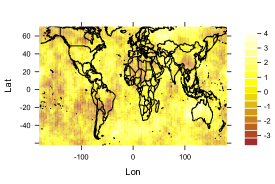
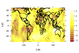
Figure 1: Simulated datasets from the $\mathcal{F}$-family with $\sigma^{2}=1$ and an approximated practical range of $4675$ kilometers. We consider $\nu=1/2$ (Left) and $\nu=5/2$ (Right). We have used the same random seed for both realisations.

3.4 Limit cases

Note how the proof of Theorem 3.1 emphasises that ${\cal F}_{\tau,\alpha,\nu}$ is the scale mixture of ${\cal N}_{\delta,\tau}$ with a Beta distribution with parameters $\alpha$ and $\nu$, where the mixture is taken with respect to $\delta\in(0,1)$. Our next result illustrates the limiting behaviour of the ${\cal F}$ covariance when $\nu,\alpha\rightarrow\infty$, in such a way that $\nu/\alpha$ is asymptotically constant.

Proposition 3.5.

Let ${\cal F}_{\tau,\alpha,\nu}$ be the family defined through (13). Let $\{\alpha_{n}\}_{n=1}^{\infty}$ and $\{\nu_{n}\}_{n=1}^{\infty}$ be two positive and increasing sequences such that $\nu_{n}/\alpha_{n}$ tends to a positive and finite constant, $\kappa$, when $n\to\infty$. Let $\mathcal{N}_{\delta,\tau}$ be the Negative Binomial family as defined in (9). Then, for each $\theta\in[0,\pi]$,

$$\mathcal{F}_{\tau,\alpha_{n},\nu_{n}}(\theta){\longrightarrow}\mathcal{N}_{1/(1+\kappa),\tau}(\theta),$$

when $n\rightarrow\infty$.

Proof. Let $\{\Delta_{n}\}_{n=1}^{\infty}$ be a sequence of random variables such that, for each $n\in\mathbb{N}$, $\Delta_{n}$ is distributed according to $\mu_{\alpha_{n},\nu_{n}}$ as defined through Equation (15). Hence,

$${\rm E}({\Delta}_{n})=\frac{1}{1+\nu_{n}/\alpha_{n}}\qquad\text{and}\qquad{\rm Var}({\Delta_{n}})=\frac{\nu_{n}/\alpha_{n}}{(1+\nu_{n}/\alpha_{n})^{2}(\alpha_{n}+\nu_{n}+1)}.$$ (34)

We invoke again the scale mixture argument in Equation (16) to write

$$\mathcal{F}_{\tau,\alpha_{n},\nu_{n}}(\theta)=\int_{0}^{1}\mathcal{N}_{\delta,\tau}(\theta)\frac{\delta^{\alpha_{n}-1}(1-\delta)^{\nu_{n}-1}}{B(\alpha_{n},\nu_{n})}\mathrm{d}\delta,\qquad\theta\in[0,\pi].\$$

Hence,

$$\lim_{n\to\infty}\mathcal{F}_{\tau,\alpha_{n},\nu_{n}}(\theta) = \lim_{n\to\infty}\int_{0}^{1}\mathcal{N}_{\delta,\tau}(\theta)\frac{\delta^{\alpha_{n}-1}(1-\delta)^{\nu_{n}-1}}{B(\alpha_{n},\nu_{n})}\mathrm{d}\delta$$ (35)

$$= \int_{0}^{1}\mathcal{N}_{\delta,\tau}(\theta)\lim_{n\to\infty}\frac{\delta^{\alpha_{n}-1}(1-\delta)^{\nu_{n}-1}}{B(\alpha_{n},\nu_{n})}\mathrm{d}\delta,$$

where the last line is justified by dominated convergence. Using the fact that $\nu_{n}/\alpha_{n}$ tends to $\kappa$, as $n\to\infty$, we have that ${\rm E}({\Delta}_{n})$ in Equation (34) tends to $1/(1+\kappa)$, whereas ${\rm Var}(\Delta_{n})$ tends to zero. This implies that the sequence of random variables $\{\Delta_{n}\}_{n=1}^{\infty}$ converges, in the mean square sense, to a random variable having a probability mass with a single atom at $1/(1+\kappa)$. This implies that the right hand side of (35) is identically equal to ${\cal N}_{1/(1+\kappa),\tau}(\theta)$. $\Box$

4 Simulation study

The ML method is generally considered best for estimating the parameters of statistical models, although the theoretical justification for this stems primarily from the asymptotic properties of ML estimators. In the present context, the study of asymptotic properties of ML estimators is complicated by the fact that the only physically sensible asymptotic regime for a process on the unit sphere is fixed domain asymptotics, i.e., increasingly dense sampling of $Z$ on its fixed domain, the unit sphere.

It is generally the case that for spatially continuous processes, under fixed domain asymptotics, prediction is consistent but parameter estimation is not (Stein, 1999). The rationale for this simulation study is therefore to explore the finite sample behaviour of ML estimates for the $\mathcal{F}$-Family of covariance functions.

A key theoretical result for fixed domain asymptotics is the equivalence of Gaussian measures associated with random fields defined over bounded sets of $\mathbb{R}^{d}$ (Skorokhod and Yadrenko, 1973). Equivalence of Gaussian measures has specific consequences for both ML estimation and for kriging predictions. First, equivalence implies that the ML estimates of the parameters of a given class of covariance functions cannot be estimated consistently. Second, the misspecified kriging predictor under the wrong covariance model is asymptotically equivalent to the kriging predictor under the true covariance. For the Matérn covariance function, using Euclidean distance and assuming the smoothing parameter to be fixed, Zhang (2004) shows that the scale and the variance cannot be estimated consistently. Instead, a specific function of the variance and the scale (called microergodic parameter – see below) can be estimated consistently.

4.1 Maximum likelihood estimates

We first study the influence of the correlation range and differentiability on the variability of the ML estimates. We parameterise the $\mathcal{F}$-Family of covariance functions as

$${\cal F}_{1/\alpha,1/\alpha+0.5,\nu}(\theta)=\sigma^{2}\frac{\Gamma(\frac{1}{\alpha}+\frac{1}{2}+\nu)\Gamma(\frac{1}{\alpha}+\nu)}{\Gamma(\frac{2}{\alpha}+\frac{1}{2}+\nu)\Gamma(\nu)}{}_{2}F_{1}\left(\frac{1}{\alpha},\frac{1}{\alpha}+\frac{1}{2},\frac{2}{\alpha}+\frac{1}{2}+\nu,\cos\theta\right),$$ (36)

with $0\leq\theta\leq\pi$. An increase in $\alpha$ corresponds to increasing the correlation range. We set $\sigma^{2}=1$ and consider four scenarios for $\alpha$ and $\nu$: (a) $(\alpha,\nu)=(0.3,0.5)$; (b) $(\alpha,\nu)=(0.6,0.5)$; (c) $(\alpha,\nu)=(0.3,2.5)$; (d) $(\alpha,\nu)=(0.6,2.5)$. Scenarios (a) and (b) correspond to a continuous, non-differentiable random field, whereas Scenarios (c) and (d) to a twice differentiable random field. Each simulated realisation generates $N=256$ data-values on a $14\times 14$ grid of longitudes and latitudes.

Figure 2 reports the centered boxplots of the ML estimates under Scenarios (a)-(d), based on 1000 independent replications. Larger values of $\alpha$ and $\nu$ correspond to higher variabilities, but there is no evidence of significant bias.

Figure 2: Centered boxplots of the ML estimates for the $\mathcal{F}$-Family under Scenarios (a)-(d), based on 1000 independent replications.

4.2 Microergodic parameter

Zhang (2004) has shown that, for the Matérn class of covariance functions as in Equation (10), not all parameters can be estimated consistently under infill asymptotics. However, using the parameterisation analogous to ours, in which $\sigma^{2}$ is the variance and $\nu$ determines the degree of mean square differentablity of the random field, the ML estimator of the microergodic parameter $\varpi=\sigma^{2}/\alpha^{2\nu}$ is consistent.

To mimic an infill asymptotic scheme, for each scenario we now generate 1000 realisations of $Z$ at $N=300,600,900,1200,1500,1800,2100$ and $2400$ locations uniformly distributed on the unit sphere, with parameter values $\sigma^{2}=1$, $\alpha=0.2$ and $\nu=1/2$. Table 1 summarises the properties of the ML estimates by their emprical bias and relative variance, i.e., the ratio between their sample variance at each value of $N$ and their sample variance when $N=300$. The biases are again negligible. The standard asymptotic result for parameter estimation is that the variance of an ML estimator is proportional to $N^{-1}$, hence the logarithm of the relative variance is linear in $\log(N)$ with slope $-1$. Figure 3 shows the empirical relationship between log-transformed relative variance and sample size from our simulation experiment. For the microergodic parameter $\varpi$, the relationship is close to linear, with estimated slope $-1.048$, whereas for $\sigma^{2}$ and $\alpha$, the estimated slopes are $-0.872$ and $-0.913$, respectively. Also, as $N$ approaches 2400, there is at least a hint that the linearity is breaking down.

In summary, the experiment suggests that ML estimates for the parameters of the $\mathcal{F}$-family behave similarly to those of the planar Matérn model under infill asymptotics.

Table 1: Bias and Relative Variance (RV) for the maximum likelihood estimates of $\sigma^{2}$, $\alpha$ and $\varpi=\sigma^{2}/\alpha^{2\nu}$ versus sample size.

		$\sigma^{2}$			$\alpha$			$\varpi$
Sample Size		Bias	RV		Bias	RV		Bias	Rel. Var.
300		$-0.00511$	1		$-0.00041$	1		$\,\,\,\,0.04908$	1
600		$-0.00044$	0.784		$\,\,\,\,0.00145$	0.661		$-0.00914$	0.393
900		$-0.00446$	0.633		$-0.00005$	0.494		$-0.00183$	0.251
1200		$-0.00147$	0.586		$\,\,\,\,0.00042$	0.404		$-0.00516$	0.171
1500		$\,\,\,\,0.00029$	0.548		$\,\,\,\,0.00052$	0.378		$-0.00054$	0.135
1800		$\,\,\,\,0.00047$	0.574		$\,\,\,\,0.00073$	0.397		$-0.00537$	0.110
2100		$\,\,\,\,0.00174$	0.520		$\,\,\,\,0.00097$	0.338		$-0.00740$	0.093
2400		$-0.00142$	0.516		$\,\,\,\,0.00009$	0.327		$-0.00228$	0.076

Figure 3: Relationship between log-transformed relative variance and sample size from our simulation experiment. Dashed, dotted and dash-dotted lines show the $\log(RV)$ for $\sigma$,$\alpha$ and $\varpi$, from the ${\cal F}$ family. The full line, added as a reference, is a line with slope -1.

5 Data illustration

We illustrate the predictive performance of the ${\cal F}$ class of covariance functions on a dataset of Precipitable Water Content (PWC) in ${\rm kg}/{\rm m}^{2}$, donwloadable at $www.esrl.noaa.gov$. This data-product is considered to be representative of the state of the Earth system (Kalnay et al., 1996) and has been used in regional studies of seasonal stream flow and water scarcity (Müller et al., 2014; Müller and Thompson, 2016). Here, we analyse the $2017$ average of PWC on a grid with spacing $2.5^{\circ}$ degrees of longitude and latitude.

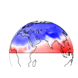
(c) Longitude $60^{\circ}$.

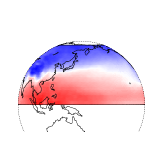
(d) Longitude $150^{\circ}$.

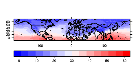
(e) Map projection of the data.

Figure 4: Plot of the data over planet Earth seen from different longitudes (4(a))–(4(d)). The whole data is depicted in (4(e)) through a map projection on the plane. The same scale was used for all panels. An animated version is available at https://github.com/FcoCuevas87/F${}\_{}$Family${}\_{}$cova.

Our study focuses on the region within latitudes $0^{\circ}$ and $70^{\circ}$ North, in order to mitigate the effect of non-stationarities over southern latitudes (Stein, 2007) and to avoid numerical instabilities around the North Pole (Castruccio and Stein, 2013). The data is shown in Figure 4, where we can observe a trend that depends on latitude. An animation is also available (see the caption of Figure 4). We remove the spatial trend through a simple harmonic regression model,

$$\mu(\bm{x})={\rm E}\left(Z(\bm{x})\right)=\eta_{0}+\eta_{1}\cos\left(\frac{\pi L}{90^{\circ}}\right)+\eta_{2}\sin\left(\frac{\pi L}{90^{\circ}}\right),$$ (37)

where $L$ denotes the latitude of the point $\bm{x}$, in degrees. Estimation was done by least squares, obtaining $\widehat{\bm{\eta}}=(\widehat{\eta}_{0},\widehat{\eta}_{1},\widehat{\eta}_{2})=(32.89,14.02,-17.65)$. Figure 5(a) shows the scatterplot of fitted values versus residuals, which suggests heteroscedasticity of the data. We then follow Verbyla (1993) and consider a log-linear model for the standard deviation:

$$\log(\sigma(L,\ell))=\gamma_{0}+\gamma_{1}\cos\left(\frac{\pi L}{90^{\circ}}\right)+\gamma_{2}\sin\left(\frac{\pi L}{90^{\circ}}\right)+\gamma_{3}\sin\left(\frac{\pi L}{90^{\circ}}\right)\sin\left(\frac{\pi\ell}{90^{\circ}}\right),$$ (38)

where $L$ and $\ell$ denote longitude and latitude, respectively. Next, we estimate the parameters of $\mu(\cdot)$ and $\sigma(\cdot,\cdot)$ using the procedures detailed in Verbyla (1993) obtaning $\widehat{\bm{\eta}}=(29.43,15.80,-13.09)$ and $(\widehat{\gamma}_{0},\widehat{\gamma}_{1},\widehat{\gamma}_{2},\widehat{\gamma}_{3})=(0.64,1.00,0.97,0.23)$. Figure 5(b) shows the scatterplot of fitted values versus residuals based on (37) and (38), whilst Figure 6 shows the residuals on planet Earth, indicating a good fit of the mean and variance functions.

To model the correlation of the residuals, we propose the following models:

1. the $\mathcal{F}$ covariance function, defined according to Equation (36).

2. the circular-Matérn covariance function (Guinness and Fuentes, 2016) given by (11). As explained in Section 2, in practice a truncation of the series expansion is needed. Therefore, we truncate the sum after $1000$ terms. Lang and Schwab (2013) adopt the same strategy and give bounds for the approximation in the mean square sense.

3. A Matérn covariance function $\mathcal{M}_{\nu,\alpha}(d_{\text{CH}})$, where $d_{\text{CH}}$ denotes the chordal distance.

For model selection purposes, we compare the performance of the proposed covariance function models with respect to ML estimation and kriging predictions. Specifically, we repeat the following two-step procedure $500$ times:

• We first sample $200$ data-locations independently at random over the region delimited by latitudes $0^{\circ}$ to $70^{\circ}$ and longitudes $-180^{\circ}$ to $120^{\circ}$. We use this data as a training set to calculate the ML estimates for each of the three models.

• Then we sample, $100$ times, $20$ data-locations in the region delimited by $0^{\circ}$ to $70^{\circ}$ in latitude and $120^{\circ}$ to $180^{\circ}$ in longitude as a validation set (see Figure 6(d)).

A similar experiment has been carried out by Jeong and Jun (2015b), who note that such a scenario may arise in practice when the interest is in predicting over the ocean but most observations are on land. Table 2 reports the average ML estimates for each model, their empirical standard errors and the maximised log-likelihood. In addition, Figure 7 shows the sample variogram and the three correlation function models using the average ML estimates. In all three cases, the estimate $\hat{\nu}$ corresponds to a continuous but nondifferentiable random field. The values of the maximised log-likelihood are very similar.

We also inspect for anisotropy of the residuals as a model validation procedure. Figure 8(a) shows the empirical semi-variogram for the filtered data together with the $2.5\%$, median and $97.5\%$ pointwise quantiles from $2499$ simulations of the fitted ${\cal F}$-family model as described below. In addition, we investigate the isotropy assumption by estimating the semi-variogram on different sub-regions of the part of the planet selected for this application. Figures 8(b) to 8(e) show the resulting semi-variograms and simulation quantiles for the data from four sub-regions defined by the combination of latitudes at north and south of $35$ degrees and longitudes at west and east of $-1$ degree. Each of these four sub-regions contains the same number of data points. The simulation quantiles were constructed using the method described in Myllymäki et al. (2017). Figure 8(a) suggests a rather poor fit, whilst Figures 8(b) to 8(e) collectively indicate non-isotropic behaviour, in that the model fit is tolerable in the first quadrant, better in the second and third quadrants, but very poor in the fourth quadrant. Similar results obtained for the circular and chordal Matérn models are available at https://github.com/FcoCuevas87/F${}\_{}$Family${}\_{}$cova.

There might be more sophisticated strategies to handle this problem: for instance, building a ${\cal F}$ class with spatially adaptive parameters to handle the differences for every subregion. In this work, we keep isotropy as in Jeong and Jun (2015b), and now focus on the predictive performance of the three models listed above.

(a) Longitude $-120^{\circ}$.

(b) Longitude $-30^{\circ}$.

(a) Constant variance.

(b) Non-constant variance

Figure 5: Residuals obtained from the regression with constant (5(a)) and non-constant (5(b)) variance.

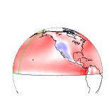
(a) Longitude $-120^{\circ}$.

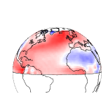
(b) Longitude $-30^{\circ}$.

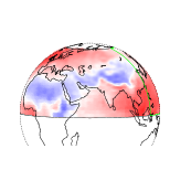
(c) Longitude $60^{\circ}$.

(d) Longitude $150^{\circ}$.

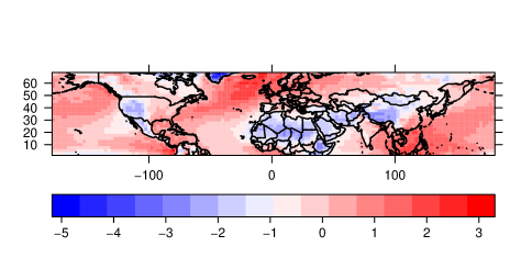
(e) Map projection of the filtered data.

Figure 6: Plot of the filtered data on planet Earth seen from different longitudes (6(a))–(6(d)). The whole set of residuals is then depicted in (6(e)) through a map projection on the plane. The same scale was used for all panels. The green region of panel (6(d)) is the window used as validation set. An animated version is available at https://github.com/FcoCuevas87/F${}\_{}$Family${}\_{}$cova.

Table 2: Average ML estimates and log-Likelihood value attained at the optimum. Standard errors are specified in parentheses.

Model	$\widehat{\sigma}_{0}$	$\widehat{\alpha}$	$\widehat{\nu}$	Log-Likelihood
$\mathcal{F}$-Family	$1.088$	$0.398$	$0.721$	$-180.963$
	(0.058)	(0.154)	(0.228)	(22.837)
Circular-Matérn	$1.110$	$0.289$	$0.665$	$-180.761$
	(0.050)	(0.088)	(0.193)	(22.905)
Matérn Chordal	$1.060$	$0.291$	$0.669$	$-180.400$
	(0.047)	(0.091)	(0.192)	(22.896)

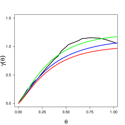
Figure 7: Empirical variogram (black) and fitted variograms with $\mathcal{F}$-family (red), chordal Matérn (green) and circular Matérn (blue).

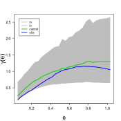
(a) Isotropic variogram using all data points.

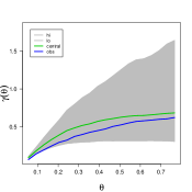
(b) Data points at south of latitude $35^{\circ}$ and west of longitude $-1^{\circ}$.

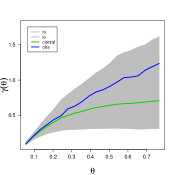
(c) Data points at south of latitude $35^{\circ}$ and east of longitude $-1^{\circ}$.

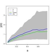
(d) Data points at north of latitude $35^{\circ}$ and west of longitude $-1^{\circ}$.

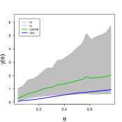
(e) Data points at north of latitude $35^{\circ}$ and east of longitude $-1^{\circ}$.

Figure 8: Empirical semi-variograms and global rank envelopes at 95% using the $\mathcal{F}$-family model with different subsets of the data (see panels). The different cut points ensure that the number of points is the same on each sub-region. The blue line represents the semi-variogram on each quadrant whilst the green line is the mean curve obtained by simulations.

In this regard, for each sample $i=1,\ldots,500,$ we calculate

$$\text{RMSE}_{i}=\frac{1}{100}\sum_{j=1}^{100}\bigg{(}\frac{1}{20}\sum_{k=1}^{20}(Z(\bm{x}_{k}^{(ij)})-\widehat{Z}(\bm{x}_{k}^{(ij)}))^{2}\bigg{)}^{1/2},$$

where $\bm{x}^{(ij)}_{k}$ is the location $k$ of the $j$-sample of the validation set for the repetition $i$, and $Z(\bm{x})$ and $\widehat{Z}(\bm{x})$ denote the true and predicted values at the site $\bm{x}$, respectively.

Figure 9 illustrates, for each model, the distribution of RMSE across the $500$ repetitions of the experiment, whilst Table 3 gives their average values. We experience that in $440$ occasions, the $\mathcal{F}$-family of covariance functions gives the lowest values. The average improvements are $2.98\%$ and $1.39\%$ in terms of relative RMSE, compared with the circular-Matérn and the chordal Matérn models, respectively.

Figure 9: Boxplot of the RMSE for each covariance model.

Table 3: RMSE averages for each covariance model based on 500 repetitions.

	$\mathcal{F}$-Family	Circular-Matérn	Matérn chordal
RMSE	$\bm{0.510}$	$0.525$	$0.517$
	(0.069)	(0.074)	(0.066)

6 Discussion

Our simulation experiment supports the view that the consistency properties of ML estimation under our proposed model mirror known results for the analagous parameterisation of the planar Matérn model. Proving this is a challenging problem. A possible approach would be to use the theory developed by Arafat et al. (2018) about equivalence of Gaussian measures on spherical spaces. This would amount to using the $d$-Schoenberg sequences associated to the ${\cal F}$ class, which are provided in Appendix A.

The reported differences in predictive performance for the PWC dataset are similar to those reported in other comparative studies (see, e.g., Gneiting et al., 2010; Jeong et al., 2018).

Stein (2007) proposes to control the latitude-dependent variance and the measurement error by augmenting the correlation function with an additive nugget effect. In our experiments, we always found that our estimates for the nugget where identically equal to zero, so that we excluded this from the presentation in Section 5.

Often, climate data are not isotropic on the sphere. In particular, Stein (2007) evokes Jones (1963) to call those covariance functions defined over $\mathbb{S}^{2}$ that are nonstationary over latitudes but stationary over longitudes axially symmetric. Appendix B shows that the ${\cal F}$-Family introduced in this paper can be used as a building block to create models that satisfy axial symmetry.

Appendices

A $d$-Schoenberg coefficients for the ${\cal F}$-family

Let $p$ and $q$ be positive integers. The generalised hypergeometric functions (Abramowitz and Stegun, 1965, 15.1.1) are defined as

$${}_{p}F_{q}{\left[\genfrac{.}{.}{0.0pt}{}{a_{1}\mskip 8.0mu\cdots\mskip 8.0mua_{p}}{b_{1}\mskip 8.0mu\cdots\mskip 8.0mub_{q}};z\right]}=\sum_{n=0}^{\infty}\frac{(a_{1})_{n}\cdots(a_{p})_{n}}{(b_{1})_{n}\cdots(b_{q})_{n}}\frac{z^{n}}{n!},\qquad|z|<1.\\$$

The special case ${}_{2}F_{1}{\left[\genfrac{.}{.}{0.0pt}{}{a\mskip 8.0mub}{c};z\right]}={}_{2}F_{1}(a,b,c;z)$ has been used in Section 3 to introduce the ${\cal F}$-Family in Equation (13).

Let $d$ be a positive integer. We now provide detailed calculations for the $d$-Schoenberg coefficients associated to (13) through the identity (6). Theorem 3.1 has provided an expression for the Schoenberg coefficients related to the Hilbert sphere $\mathbb{S}^{\infty}$.

Property A.1 Let ${\cal F}_{\tau,\alpha,\nu}$ be the family of functions defined through Equation (13). Let $d$ be a positive integer. Then, the $d$-Schoenberg sequence of coefficients $\{b_{n,d}\}_{n=0}^{\infty}$ related to ${\cal F}_{\tau,\alpha,\nu}$ through Equation (6) are uniquely determined by

$$b_{n,d}=\left\{\begin{array}[]{cc}K_{even}(\alpha,\tau,\nu,n,d){}_{5}F_{4}{\left[\genfrac{.}{.}{0.0pt}{}{\frac{\alpha}{2}+n\mskip 8.0mu\frac{\alpha+1}{2}+n\mskip 8.0mu\frac{\tau}{2}+n\mskip 8.0mu\frac{\tau+1}{2}+n\mskip 8.0mu1}{\frac{\alpha+\nu+\tau}{2}+n\mskip 8.0mu\frac{\alpha+\nu+\tau+1}{2}+n\mskip 8.0mu\frac{n}{2}+1\mskip 8.0mu\frac{3n+d+1}{2}};1\right]}&\mbox{ if n is even},\\ &\\ &\\ K_{odd}(\alpha,\tau,\nu,n,d){}_{5}F_{4}{\left[\genfrac{.}{.}{0.0pt}{}{\frac{\alpha}{2}+n+1\mskip 8.0mu\frac{\alpha+1}{2}+n\mskip 8.0mu\frac{\tau+1}{2}+n\mskip 8.0mu\frac{\tau}{2}+n+1\mskip 8.0mu1}{\frac{\alpha+\nu+\tau+1}{2}+n\mskip 8.0mu\frac{\alpha+\nu+\tau}{2}+n+1\mskip 8.0mu\frac{n+3}{2}\mskip 8.0mu\frac{3n+d+2}{2}};1\right]}&\mbox{ if n is odd},\end{array}\right.$$

where

$$K_{even}(\alpha,\tau,\nu,n,d)=\frac{B(\alpha,\nu+\tau)}{B(\alpha,\nu)}\frac{(\alpha)_{2n}(\tau)_{2n}(2n+d-1)\Gamma\left(\frac{d-1}{2}\right)}{(\alpha+\nu+\tau)_{2n}2^{2n+1}\Gamma\left(\frac{n+2}{2}\right)\Gamma\left(\frac{3n+d+1}{2}\right)}{{n+d-2}\choose{n}},$$

and

$$K_{odd}(\alpha,\tau,\nu,n,d)=\frac{B(\alpha,\nu+\tau)}{B(\alpha,\nu)}\frac{(\alpha)_{2n+1}(\tau)_{2n+1}(2n+d-1)\Gamma\left(\frac{d-1}{2}\right)}{(\alpha+\nu+\tau)_{2n+1}2^{2n+2}\Gamma\left(\frac{n+3}{2}\right)\Gamma\left(\frac{3n+d+2}{2}\right)}{{n+d-2}\choose{n}}.$$

Proof. The proof of Theorem 3.1 has shown that the Schoenberg coefficients related to the $\Psi_{\infty}$ representation of the family ${\cal F}$ are defined by

$$b_{n}=\frac{B(\alpha,\nu+\tau)}{B(\alpha,\nu)}\frac{(\alpha)_{n}(\tau)_{n}}{(\alpha+\nu+\tau)_{n}(n!)}.$$ (A.1)

Theorem 4.1 in Møller et al. (2018) shows that, since the function ${\cal F}_{\tau,\alpha,\nu}$ belongs to the class $\Psi_{\infty}$, its $d$-Schoemberg coefficients $b_{n,d}$ are uniquely determined through

$$b_{n,d}=\sum_{\begin{subarray}{c}l=n\\ n-l\equiv 0(\mod 2)\end{subarray}}^{\infty}b_{n}\gamma_{n,l}^{(d)}$$ (A.2)

where $b_{n}$ is defined in (A.1) and

$$\gamma_{n,l}^{d}=\frac{(2n+d-1)(l!)\Gamma\left(\frac{d-1}{2}\right)}{{2^{l+1}\left\{\left(\frac{l-n}{2}\right)!\right\}\Gamma\left(\frac{l+n+d+1}{2}\right)}}{{n+d-2}\choose{n}}.$$

We can now plugin (A.1) into (A.2) to get

$$b_{n,d} =K_{1}(\alpha,\tau,\nu,n,d)\sum_{\begin{subarray}{c}l=n\\ n-l\equiv 0(\mod 2)\end{subarray}}\frac{(\alpha)_{l}(\tau)_{l}}{(\alpha+\nu+\tau)_{l}2^{l+1}\left\{\left(\frac{l-n}{2}\right)!\right\}\Gamma\left(\frac{l+n+d+1}{2}\right)}\noindent$$

$$=K_{1}(\alpha,\tau,\nu,n,d)S_{n}(\alpha,\tau,\nu,n,d),$$

where

$$K_{1}(\alpha,\tau,\nu,n,d)=(2n+d-1)\Gamma\left(\frac{d-1}{2}\right){{n+d-2}\choose{n}}\frac{B(\alpha,\nu+\tau)}{B(\alpha,\nu)}.$$

When $n$ is an even positive integer, we get that

$$S_{n}(\alpha,\tau,\nu,n,d)=\sum_{j=n}^{\infty}\frac{(\alpha)_{2j}(\tau)_{2j}}{(\alpha+\nu+\tau)_{2j}2^{2j+1}\left\{\left(\frac{2j-n}{2}\right)!\right\}\Gamma\left(\frac{2j+n+d+1}{2}\right)}.$$

We now define $i=j-n$ to obtain

$$S_{n}(\alpha,\tau,\nu,n,d)=\sum_{i=0}^{\infty}\frac{(\alpha)_{2i+2n}(\tau)_{2i+2n}}{(\alpha+\nu+\tau)_{2i+2n}2^{2i+2n+1}\left\{\left(i+\frac{n}{2}\right)!\right\}\Gamma\left(i+\frac{3n+d+1}{2}\right)}.$$

We can now make use of the factorisation $(\alpha)_{2i+2n}=(\alpha)_{2n}(a+n)_{2i}$ (Prudnikov et al., 1983) to obtain

$$S_{n}(\alpha,\tau,\nu,n,d)=\frac{(\alpha)_{2n}(\tau)_{2n}}{(\alpha+\nu+\tau)_{2n}2^{2n+1}}\sum_{i=0}^{\infty}\frac{(\alpha+n)_{2i}(\tau+n)_{2i}}{(\alpha+\nu+\tau+n)_{2i}2^{2i+1}\left\{\left(i+\frac{n}{2}\right)!\right\}\Gamma\left(i+\frac{3n+d+1}{2}\right)}.$$

Using the dimidiation formula for the Pochhammer symbol (Prudnikov et al., 1983)

$$(\alpha)_{2i}=2^{2i}(\alpha/2)_{i}((\alpha+1)/2)_{i},$$

and completing terms, the series $S_{n}$ is

$$S_{n}(\alpha,\tau,\nu,n,d) =K_{2}(\alpha,\tau,\nu,n,d)\sum_{i=0}^{\infty}\frac{(\frac{\alpha+1}{2}+n)_{i}(\frac{\alpha}{2}+n)_{i}(\frac{\tau}{2}+n)_{i}(\frac{\tau+1}{2}+n)_{i}(1)_{i}}{\left(\frac{\alpha+\nu+\tau}{2}+n\right)_{i}(\frac{\alpha+\nu+\tau+1}{2}+n)_{i}\left(\frac{n}{2}+1\right)_{i}\left(\frac{3n+d+1}{2}\right)_{i}i!},$$

$$=K_{2}(\alpha,\tau,\nu,n,d){}_{5}F_{4}{\left[\genfrac{.}{.}{0.0pt}{}{\frac{\alpha}{2}+n\mskip 8.0mu\frac{\alpha+1}{2}+n\mskip 8.0mu\frac{\tau}{2}+n\mskip 8.0mu\frac{\tau+1}{2}+n\mskip 8.0mu1}{\frac{\alpha+\nu+\tau}{2}+n\mskip 8.0mu\frac{\alpha+\nu+\tau+1}{2}+n\mskip 8.0mu\frac{n}{2}+1\mskip 8.0mu\frac{3n+d+1}{2}};1\right]},$$

where

$$K_{2}(\alpha,\tau,\nu,n,d)=\frac{\left(\alpha\right)_{2n}(\tau)_{2n}}{(\alpha+\nu+\tau)_{2n}2^{2n+1}\Gamma\left(\frac{n}{2}\right)\Gamma\left(\frac{3n+d+1}{2}\right)},$$

and

$$K_{even}(\alpha,\tau,\nu,n,d)=K_{1}(\alpha,\tau,\nu,n,d)K_{2}(\alpha,\tau,\nu,n,d).$$

When $n$ is an odd positive integer, the proof works mutatis mutandis through similar calculations $\Box$

B Axially symmetric version of the ${\cal F}$ class

For phenomena covering a big portion of our planet, isotropy is a questionable assumption. On the one hand, isotropy might be expected for microscale metereology on a sufficiently temporally aggregated level for many physical quantities. On the other hand, mesoscale and synoptic scale meteorology are not even approximately isotropic, due to the highly nonlinear nature of the Earth’s system. Indeed, Stein (2007) shows that total column ozone data show significant changes over latitude. Castruccio and Stein (2013) argued that both inter and intra annual variability for surface temperature is depend on latitude. For the sequel, we refer to the unit sphere $\mathbb{S}^{2}$ of $\mathbb{R}^{3}$ with coordinates $\bm{x}=(L,\ell)^{\top}$, with $L\in[0,\pi]$ denoting latitude and $\ell\in[0,2\pi)$ denoting longitude. In particular, Stein (2007) resorts to the results in Jones (1963) to call the covariance $C$ axially symmetric when

$$C\left(\bm{x}_{1},\bm{x}_{2}\right)={\cal C}(L_{1},L_{2},\ell_{1}-\ell_{2}),\qquad(L_{i},\ell_{i})\in[0,\pi]\times[0,2\pi),i=1,2.$$

Axially symmetric processes have a well understood spectral representation that includes as a special case the geodesic isotropy illustrated through Equations (3) and (4). For details, the reader is referred to Jones (1963) and more recently to Stein (2007).

The literature on axially symmetric models is sparse, with the attempt in Porcu et al. (2019) being a notable exception. Let $d_{{\rm CH}}(\ell_{1},\ell_{2})$ denote the chordal distance between two longitudes $\ell_{1}$ and $\ell_{2}$. Let ${\cal M}_{\alpha,\nu}$ denote the Matérn class defined at (10). Then, Porcu et al. (2019) propose an axially symmetric model of the type

$${\cal C}(L_{1},L_{2},\ell_{1}-\ell_{2})=\sigma(L_{1},L_{2}){\cal M}_{\alpha(L_{1},L_{2}),\nu(L_{1},L_{2})}\left(d_{{\rm CH}}(\ell_{1},\ell_{2})\right),$$

$(L_{i},\ell_{i})\in[0,\pi]\times[0,2\pi),i=1,2$, where $\sigma,\alpha$ and $\nu$ are strictly positive functions that must be carefully chosen in order to preserve positive definiteness. The interpretation of these functions is very intuitive, as they indicate how, respectively, variance, scale and smoothness can vary across latitudes. Usually $\sigma$ is modeled through a linear combination of Legendre polynomials (Jun and Stein, 2007). To illustrate the new model, we need to define a stochastic process $\{X(L),\;L\in[0,\pi]\}$ and we call variogram the quantity ${\rm Var}\left(X(L_{2})-X(L_{1})\right)/2$, $L_{1},L_{2}\in[0,\pi]$ (see Chiles and Delfiner, 1999, with the references therein).

Theorem B.1 Let ${\cal F}$ be the family of functions defined at Equation (13). Let $\tau>0$. Let $\sigma:[0,\pi]^{2}\to\mathbb{R}_{+}$ be positive definite and let $\alpha,\nu:[0,\pi]^{2}\to\mathbb{R}_{+}$ be continuous functions such that the functions $(L_{1},L_{2})\mapsto{\alpha(L_{1},L_{2})}$ and $(L_{1},L_{2})\mapsto{\nu(L_{1},L_{2})}$ define two variograms on $[0,\pi]^{2}$. Then, the function

$${\cal C}(L_{1},L_{2},\ell_{1}-\ell_{2})=\sigma(L_{1},L_{2}){\cal F}_{\tau,\alpha(L_{1},L_{2}),\nu(L_{1},L_{2})}\left(\theta(\ell_{1},\ell_{2})\right),$$

for $(L_{i},\ell_{i})\in[0,\pi]\times[0,2\pi)$, is positive definite.

Proof. We give a constructive proof. We consider the scale mixture

$$\int_{0}^{1}\frac{(1-\delta)^{\tau}}{\left(1-\delta\cos\theta(\ell_{1},\ell_{2})\right)^{\tau}}\delta^{\alpha(L_{1},L_{2})-1}(1-\delta)^{\nu(L_{1},L_{2})-1}{\rm d}\delta.$$

Clearly, the function $(\ell_{1},\ell_{2})\mapsto(1-\delta)^{\tau}/(1-\delta\cos\theta(\ell_{1},\ell_{2}))^{\tau}$ is positive definite for any $\tau>0$ and $\delta\in(0,1)$. Both functions $a^{\alpha}$ and $a^{\nu}$ are positive definite on $[0,\pi]^{2}$ provided $0\leq a\leq 1$ (direct consequence of Schoenberg, 1942, Theorem 2). Since the scale mixture above is well defined, the proof is completed by using the same arguments as in Theorem 3.1. $\Box$

References

- Abramowitz and Stegun (1965) Abramowitz, M. and I. Stegun (1965). Handbook of Mathematical Functions: with Formulas, Graphs, and Mathematical Tables, Volume 55. Courier Corporation.
- Arafat et al. (2018) Arafat, A., E. Porcu, M. Bevilacqua, and J. Mateu (2018). Equivalence and orthogonality of Gaussian measures on spheres. Journal of Multivariate Analysis 267, 306–318.
- Banerjee (2005) Banerjee, S. (2005). On geodetic distance computations in spatial modeling. Biometrics 61, 617–625.
- Beatson et al. (2014) Beatson, R. K., W. zu Castell, and Y. Xu (2014). Pólya criterion for (strict) positive definiteness on the sphere. IMA Journal of Numerical Analysis 34, 550–568.
- Berg and Porcu (2017) Berg, C. and E. Porcu (2017). From Schoenberg coefficients to Schoenberg functions. Constructive Approximation 45, 217–241.
- Bevilacqua et al. (2012) Bevilacqua, M., C. Gaetan, J. Mateu, and E. Porcu (2012). Estimating space and space-time covariance functions: a weighted composite likelihood approach. Journal of the American Statistical Association 107, 268–280.
- Castruccio and Stein (2013) Castruccio, S. and M. L. Stein (2013). Global space-time models for climate ensembles. Annals of Applied Statistics 7, 1593–1611.
- Chiles and Delfiner (1999) Chiles, J. and P. Delfiner (1999). Geostatistics: Modeling Spatial Uncertainty. New York: Wiley.
- Daley and Porcu (2013) Daley, D. J. and E. Porcu (2013). Dimension walks and Schoenberg spectral measures. Proceedings of the American Mathematical Society 141, 1813–1824.
- Furrer et al. (2006) Furrer, R., M. G. Genton, and D. Nychka (2006). Covariance tapering for interpolation of large spatial datasets. Journal of Computational and Graphical Statistics 15, 502–523.
- Galassi et al. (1996) Galassi, M., J. Davies, J. Theiler, B. Gough, G. Jungman, P. Alken, M. Booth, and F. Rossi (1996). GNU scientific library reference manual.
- Gneiting (2013) Gneiting, T. (2013). Strictly and non-strictly positive definite functions on spheres. Bernoulli 19, 1327–1349.
- Gneiting et al. (2010) Gneiting, T., W. Kleiber, and M. Schlather (2010). Matérn cross-covariance functions for multivariate random fields. Journal of the American Statistical Association 105(491), 1167–1177.