Nonlinear saturation of thermal instabilities

Abstract

Low-frequency simulations of a one-layer model with lateral buoyancy variations (i.e., thermodynamically active) have revealed circulatory motions resembling quite closely submesoscale observations in the surface ocean rather than indefinitely growing in the absence of a high-wavenumber instability cutoff. In this note it is shown that the existence of a convex pseudoenergy–momentum integral of motion for the inviscid, unforced dynamics provides a mechanism for the nonlinear saturation of such thermal instabilities in the zonally symmetric case. The result is an application of Arnold [3] and Shepherd [44] methods.

I Introduction

A simple recipe, introduced in as early as at least the late 1960s [28], to incorporate thermodynamic processes (e.g., those due to heat and freshwater exchanges through the air–sea interface) in a one-layer ocean model consisted in allowing buoyancy to vary with horizontal position and time, while keeping velocity as independent of the vertical coordinate. The simplicity of the resulting inhomogeneous-layer model with fields that do not change with depth—referred to as IL⁰ by Ripa [36, 37, 41] to reflect this—promised fundamental understanding of ocean processes which would be difficult to gain by analyzing direct observations or the output from an ocean general circulation model. A number of applications of the IL⁰, particularly to equatorial dynamics, appeared in the 1980s and 1990s supporting this line of thought [42, 1, 22, 4].

Regrettably, the increase in computational power in the current century has led to overemphasize reproducing observations in detriment of gaining basic physical insight of the type that ocean modeling based on the IL⁰ system or variants thereof [50, 37, 5, 7] was expected to provide. A pleasant surprise, however, has been to learn that layer ocean modeling with reduced thermodynamics is regaining momentum [52, 15, 20, 25]. Moreover, the renewed interest in this type of modeling is exceeding a pure oceanographic interest. Indeed, applications of the IL⁰ have been extended to atmospheric dynamics, both terrestrial [19] (beyond the original one [21]) and planetary [47, 48].

Of particular interest to the present work are the numerical simulations of the IL⁰ by Holm, Luesink, and Pan [15], which have shown that it can sustain subinertial (i.e., with frequency smaller than the local Coriolis parameter, twice the local Earth’s rotation rate) circulatory motions (cf. Fig. 1) that resemble quite well submesoscale (1–10 km) features often observed in satellite ocean color images. This note is concerned with identifying a mechanism that can prevent such thermal instabilities [13] from growing indefinitely in the absence of a high-wavenumber cutoff in the IL⁰ model [12, 51, 38].

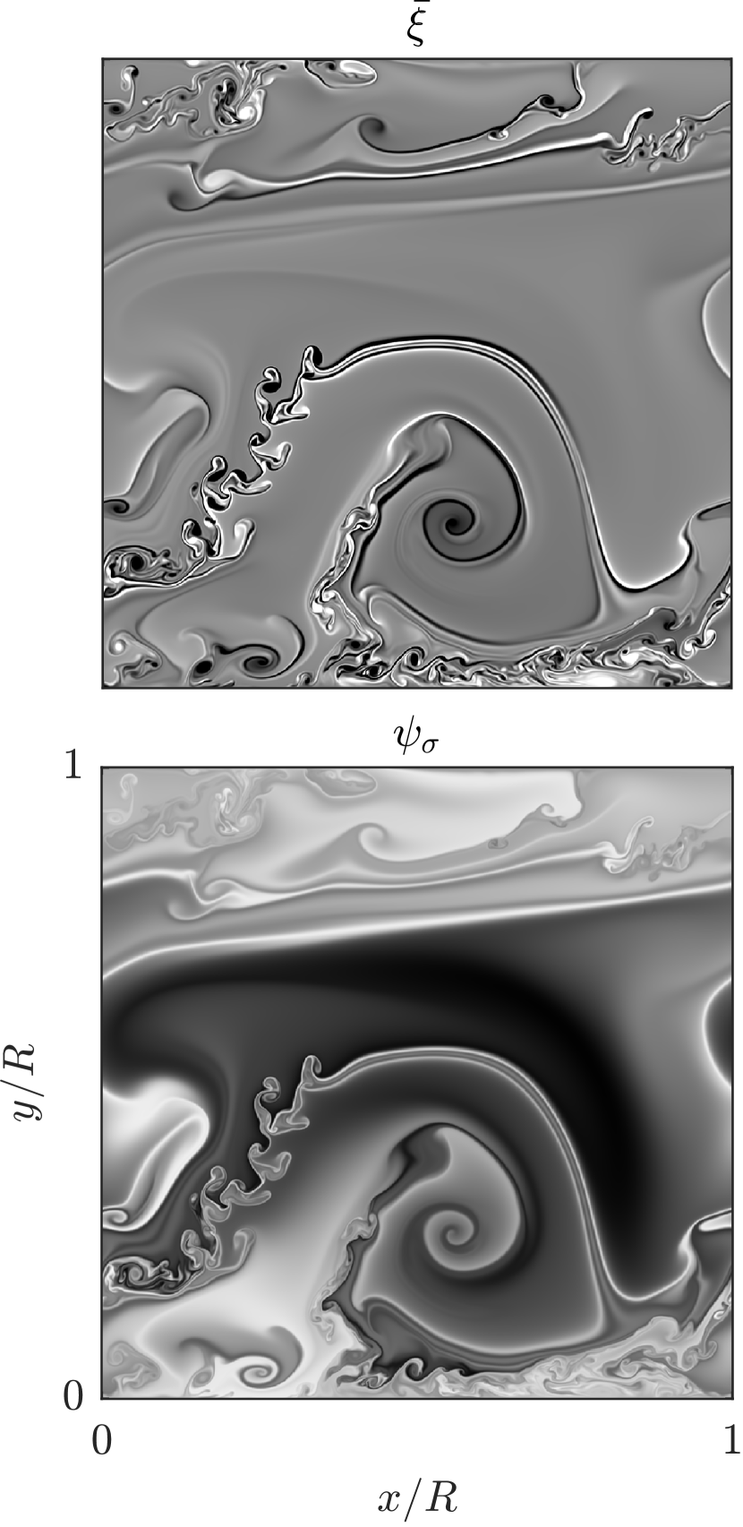
Figure 1: Snapshot of potential vorticity (top) and buoyancy excess (bottom) from a numerical solution of system (1b) initialized close to an unstable uniform zonal flow in a periodic channel of the $\beta$-plane using a pseudospectral code [8] on a $1024^{2}$-resolution grid. Note the Kelvin–Helmholtz-like rollups with scales much smaller than the deformation radius ($R$) of the problem.

II A quasigeostrophic IL⁰

Consider a low-frequency approximation to the IL⁰ model in a reduced-gravity setting (i.e., with the active layer floating atop a quiescent, infinitely deep layer of constant density), which is most appropriate to study near-surface (mixed-layer) ocean processes. Let $x$ (resp., $y$) point eastward (resp., northward) on a zonal $\beta$-plane [32] channel, $L$-periodic and of width $W$. The quasigeostrophic IL⁰ takes the form [41]

$$\partial_{t}\bar{\xi}+[\bar{\psi},\bar{\xi}]=R^{-2}[\bar{\psi},\psi_{\sigma}],\quad\partial_{t}\psi_{\sigma}+[\bar{\psi},\psi_{\sigma}]=0,$$ (1a)

with invertibility principle

$$\nabla^{2}\bar{\psi}-R^{-2}\bar{\psi}=\bar{\xi}-R^{-2}\psi_{\sigma}-\beta y,$$ (1b)

all subjected to no-flow through the coasts, $\smash{\partial_{x}\bar{\psi}|_{y=0,W}}=0$, constancy of Kelvin circulations along them, $-\smash{\int_{0}^{L}\partial_{y}\bar{\psi}|_{y=0,W}}\operatorname{d}\!{x}=\gamma_{0,W}=\mathrm{const}$, and $L$-periodicity in $x$. In (1b), $[\,,]$ is the canonical Poisson bracket (Jacobian) in $\mathbb{R}^{2}\{x,y\}$ and $R:=\smash{\frac{\sqrt{g_{\mathrm{b}}H_{\mathrm{r}}}}{|f_{0}|}}>0$ is the Rossby deformation radius, where $g_{\mathrm{b}}>0$ is the reference (i.e., in the absence of currents) buoyancy of the active (relative to the passive) layer whose thickness is $H_{\mathrm{r}}>0$, and $f_{0}$ is the Coriolis parameter at the southern coast (its dependence on latitude is represented by $f_{0}+\beta y$). The instantaneous layer thickness, buoyancy, and velocity, $h=H_{\mathrm{r}}\smash{\big{(}1+\frac{\bar{\psi}-\psi_{\sigma}}{f_{0}R^{2}}\big{)}}$, $\vartheta=g_{\mathrm{b}}\smash{\big{(}1+2\frac{\psi_{\sigma}}{f_{0}R^{2}}\big{)}}$, and $\mathbf{u}=\nabla^{\perp}\bar{\psi}$, respectively. Alternative forms of (1b) are presented in Ripa [39], Warnerford and Dellar [49], Holm, Luesink, and Pan [15]

The quantity $\bar{\xi}$ in (1b) is a quasigeostrophic approximation to the vertically averaged Ertel’s potential vorticity [37], which is not a Lagrangian constant of the model. This justifies the overbar notation. Note that by the thermal-wind balance, which is not explicitly resolved, $\mathbf{u}$ would have a vertical shear proportional to $\nabla^{\perp}\psi_{\sigma}$. In order for $\mathbf{u}$ to read as above upon a vertical average over $-h\leq z\leq 0$, it should be of the form $\mathbf{u}=\nabla^{\perp}\bar{\psi}+\sigma\nabla^{\perp}\psi_{\sigma}$, where $\sigma=1+\frac{2z}{h}$, which justifies the $\sigma$ subscript (cf. Ripa [41] for details).

System (1b) preserves energy,

$$\mathcal{E}:=\tfrac{1}{2}\int|\nabla\bar{\psi}|^{2}+R^{-2}\bar{\psi}^{2}$$ (2)

(where $\int$ is a short-hand notation for integration over the zonal-channel domain and operates on everything on its right); an infinite family of Casimirs,

$$\mathcal{C}:=a_{0}\gamma_{0}+a_{W}\gamma_{W}+\int C_{1}(\psi_{\sigma})+\bar{\xi}C_{2}(\psi_{\sigma})$$ (3)

with $a_{0,W}=\mathrm{const}$ and $C_{1},C_{2}(\,)$ arbitrary; and zonal momentum

$$\mathcal{M}:=\int y\bar{\xi}.$$ (4)

Furthermore, in Ripa [39] it is shown that equations (1b) possess a generalized Hamiltonian structure [26] on the state variables $(\bar{\xi},\bar{\psi},\gamma_{0,W})$ with Hamiltonian given by (2) and Lie–Poisson bracket $\{\mathcal{F},\mathcal{G}\}:=\smash{\int\bar{\xi}\big{[}\frac{\delta\mathcal{F}}{\delta\bar{\xi}},\frac{\delta\mathcal{G}}{\delta\bar{\xi}}\big{]}+\psi_{\sigma}\big{[}\frac{\delta\mathcal{F}}{\delta\bar{\xi}},\frac{\delta\mathcal{G}}{\delta\psi_{\sigma}}\big{]}+\psi_{\sigma}\big{[}\frac{\delta\mathcal{F}}{\delta\psi_{\sigma}},\frac{\delta\mathcal{G}}{\delta\bar{\xi}}\big{]}}$ for admissible functionals of state $\mathcal{F},\mathcal{G}$. (The variational derivative of a functional $\smash{\mathcal{F}[\varphi]=\int F(x,y,t;\varphi,\partial_{x}\varphi,\partial_{y}\varphi,\partial_{xy}\varphi,\dotsc})$ is the unique element $\smash{\frac{\delta\mathcal{F}}{\delta\varphi}}$ satisfying $\smash{\left.\frac{\operatorname{d}\!{}}{\operatorname{d}\!{\varepsilon}}\right|_{\varepsilon=0}\mathcal{F}[\varphi+\varepsilon\delta\varphi]=\int\frac{\delta\mathcal{F}}{\delta\varphi}\,\delta\varphi}$.) The admissibility condition for the zonal-channel domain is $\smash{\partial_{x}\frac{\delta\mathcal{F}}{\delta\bar{\xi}}|_{y=0,W}=0=\partial_{x}\frac{\delta\mathcal{F}}{\delta\psi_{\sigma}}|_{y=0,W}}$. This bracket turns out to be the same as that for “low-$\beta$” reduced magnetohydrodynamics [27] and incompressible, nonhydrostatic, Boussinesq fluid dynamics on a vertical plane [6]; so the Casimirs in (3), satisfying $\{\mathcal{F},\mathcal{C}\}=0$ for all $\mathcal{F}$, have been known prior to the derivation of the derivation of (1b). These integrals play a critical role in the derivation of a-priori stability criteria, discussed below. The Hamiltonian formalism enables the linkage of conservation laws with symmetries via Noether’s theorem (e.g., Shepherd [46]). From a more practical fluid dynamics standpoint, it provides a framework for deriving flow-topology-preserving stochastic versions [14, 15] of a generalized Hamiltonian model from its analogous Euler–Poincare variational formulation [16], which can be used to build parametrizations of unresolvable subgrid-scale motions [11].

III Stability/instability

Let capital letters denote variables that define a basic state for (1b), i.e., a steady solution or equilibrium to (1b) with currents. An example is the uniform zonal flow, defined by

$$\bar{\Psi}=-\bar{U}y,\quad\Psi_{\sigma}=-U_{\sigma}y,$$ (5)

where $\bar{U},U_{\sigma}$ are constants, with $U_{\sigma}<\smash{\frac{f_{0}R^{2}}{2W}}$ so $\Theta=g_{\mathrm{b}}\smash{\big{(}1-\frac{2U_{\sigma}}{f_{0}R^{2}}y\big{)}}>0$. Note that, from the thermal-wind relation, a basic state with the latter buoyancy distribution would be consistent with a zonal flow with uniform vertical shear given by $\smash{\frac{2U_{\sigma}}{H_{\mathrm{r}}}}$. Thus the study of perturbations to (5) represents, implicitly, a baroclinic instability problem of the free-boundary type studied in Beron-Vera and Ripa [10]. As opposed to classical baroclinic instability [32], free boundary baroclinic instability has a soft interface, which has a slope, given by $\smash{\frac{(U_{\sigma}-\bar{U})H_{\mathrm{r}}}{f_{0}R^{2}}}$, in the basic state. The phase speed of infinitesimal normal-mode perturbations to (5) is given by

$$c-\bar{U}=-\frac{\bar{U}+U_{\sigma}+\beta R^{2}}{2|\mathbf{k}|^{2}R^{2}+2}\pm\frac{\sqrt{(\bar{U}+U_{\sigma}+\beta R^{2})^{2}-4\bar{U}U_{\sigma}(|\mathbf{k}|^{2}R^{2}+1)}}{2|\mathbf{k}|^{2}R^{2}+2},$$ (6)

which extends the result of Ripa [37], Young and Chen [51] to the $\beta$-plane. A sufficient condition for the absence of growing normal modes is

$$\frac{\bar{U}}{U_{\sigma}}<0.$$ (7)

In Fig. 2 I show, as a function of $\smash{\frac{\bar{U}}{U_{\sigma}}}$, the minimum wavenumber $|\mathbf{k}|$ for instability for various $\smash{\frac{\beta R^{2}}{U_{\sigma}}}$ values. Note that there is stability for $\smash{\frac{\bar{U}}{U_{\sigma}}}<0$ for all $|\mathbf{k}|$, as expected. While $\beta$ can have a stabilizing effect, the lack of a high-wavenumber cutoff of instability when $\smash{\frac{\bar{U}}{U_{\sigma}}}>0$ can be consequential for the nonlinear evolution of system (1b), which however tends to show Kelvin–Helmoltz-like circulations that saturate at subdeformation scales rather than blowing up indefinitely [15].

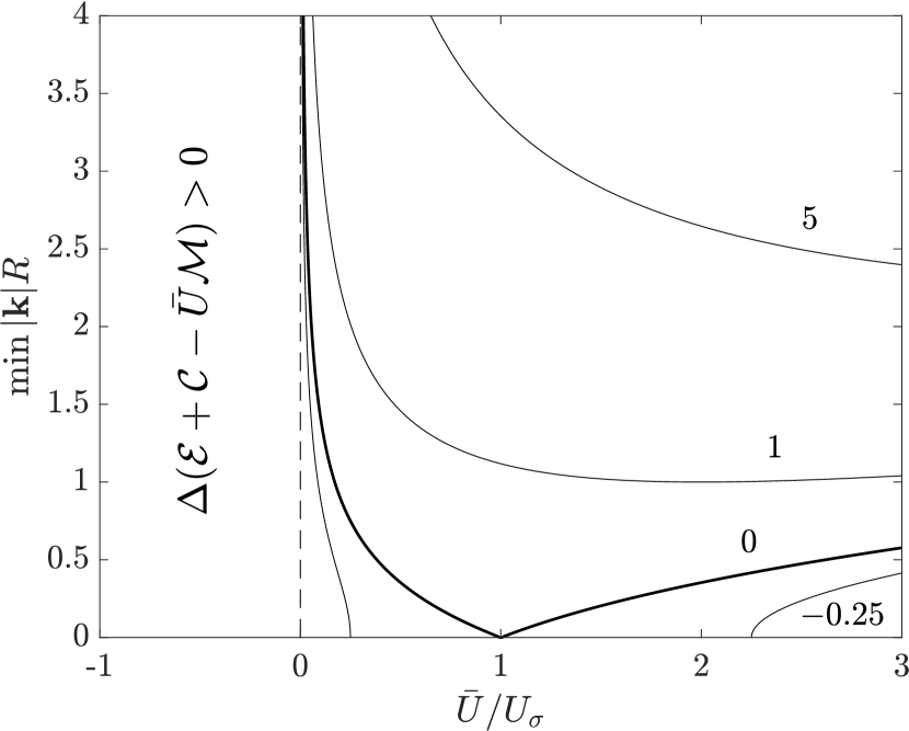
Figure 2: Minimum wavenumber for instability of a uniform zonal current for various $\smash{\frac{\beta R^{2}}{U_{\sigma}}}$ values.

Condition (7) was shown in Ripa [39] to be an a-priori condition for the formal stability of basic state (5), i.e., stability under small-amplitude perturbations of arbitrary structure. This result followed from the application of Arnold [2] method. This consists in constructing an integral of motion which is quadratic to the lowest order on the deviation from a basic state and either is positive-definite (Arnold’s first theorem) or negative-definite (Arnold’s second theorem) (cf. Holm et al. [17], McIntyre and Shepherd [23]). In both cases, the integral represents a norm that constrains the growth of perturbations. For the zonally symmetric basic state (5), such an integral of motion is given by

$$\delta^{2}\mathcal{H}_{\bar{U}}:=\delta^{2}(\mathcal{E}+\mathcal{C}-\bar{U}\mathcal{M})=\tfrac{1}{2}\int|\nabla\delta\bar{\psi}|^{2}+R^{-2}\left(\delta\bar{\psi}^{2}-\frac{\bar{U}}{U_{\sigma}}\delta\psi_{\sigma}^{2}\right)$$ (8)

for $\mathcal{C}$ in (3) with $C_{1}=-\frac{\bar{U}}{2R^{2}U_{\sigma}}\psi_{\sigma}^{2}$ and $C_{2}=0$ so $\delta\mathcal{H}_{\bar{U}}=0$. Note that (8) is positive-definite when (7) holds. (That the circulation perturbations $\delta\gamma_{0,W}$ do not enter in (8) should not be taken as implying positive-semidefinitness of (8) and hence the possibility of unarrested growth along their directions in phase space: once initially specified, $\delta\gamma_{0,W}$ remain the same at all times. Also note that when $R\to\infty$, i.e., the interface is rigid, system (1b) reduces to $\partial_{t}\bar{\xi}+[\bar{\psi},\bar{\xi}]=0$ with $\nabla^{2}\bar{\psi}=\bar{\xi}-\beta y$, for which $\bar{\Psi}=-\bar{U}y$ clearly is stable consistent with (8) being positive-definite in this limit.) Furthermore, (8) coincides with the pseudoenergy–momentum $\Delta\mathcal{H}_{\bar{U}}$, which is an exact integral of motion of (1b). Indeed, $\mathcal{H}_{\alpha}$ is a Hamiltonian for the motion as viewed from an $x$-translating frame at constant speed $\alpha$. This shows that (7) actually is a condition for the formal stability of (5) under finite-amplitude perturbations. However, (8) cannot be proved to be convex, i.e., to be bounded from below and above by multiples of an L²-norm on the perturbation field. This precludes one from declaring (5) stable in a Lyapunov sense [3] when (7) holds, i.e., the L²-distance of a perturbation to (5) cannot be bounded at all times by a multiple of the initial distance (cf. Holm et al. [17], McIntyre and Shepherd [23]). Finally, the possibility of proving stability when (7) is violated by seeking conditions under which (8) is negative-definite, namely, conditions under which $\delta^{2}\mathcal{E}=\smash{\frac{1}{2}\int|\nabla\delta\bar{\psi}|^{2}+R^{-2}\delta\bar{\psi}^{2}}$ can be bounded by $-\delta^{2}\mathcal{C}=\smash{\frac{1}{2}R^{-2}\frac{\bar{U}}{U_{\sigma}}\int\delta\psi_{\sigma}^{2}}$, is ruled out because $\delta\bar{\psi}$ is not a (nonlocal) function of $\delta\psi_{\sigma}$ exclusively. (On the invariant subspace of system (1b), given by $\{\psi_{\sigma}=\mathrm{const}\}$, $\delta\bar{\psi}=(\nabla^{2}-R^{-2})^{-1}\delta\bar{\xi}$. Thus on that subspace, relative to a general sheared zonal flow $\bar{\Psi}=-\int^{y}\bar{\mathscr{U}}(y)$, both positive and negative pseudoenergy–momentum integrals exist provided that for all $y\in[0,W]$ there are constants $\alpha$ such that $\smash{\frac{\bar{\mathscr{U}}(y)-\alpha}{\beta-\bar{\mathscr{U}}^{\prime\prime}(y)+R^{-2}\bar{\mathscr{U}}^{\prime}(y)}}$ is negative and bigger than $(\kappa^{2}+R^{-2})^{-1}$, respectively, where $\kappa^{2}$ is the gravest eigenvalue of the Helmholtz equation with zero Dirichlet boundary conditions at $y=0,W$; cf. Ripa [33, 35].)

IV Instability saturation

The fact that the pseudoenergy–momentum (8) is not convex appears to conspire against the purpose here to bound the growth of perturbations to an unstable basic state, for which (7) is necessary violated. Let $\varphi$ denote the state vector. Let the superscript S (resp., U) indicate stable (resp., unstable). Assume that the following convexity estimate holds: $a(\Phi^{\mathrm{S}})\smash{\|\varphi-\Phi^{\mathrm{S}}\|_{t=t_{0}}}\leq\|\varphi-\Phi^{\mathrm{S}}\|\leq A(\Phi^{\mathrm{S}})\smash{\|\varphi-\Phi^{\mathrm{S}}\|_{t=t_{0}}}$ for $0<a(\Phi^{\mathrm{S}})\leq A(\Phi^{\mathrm{S}})<\infty$ and $\|\,\|$ representing a certain L²-norm. Then one finds: $\|\varphi-\Phi^{\mathrm{U}}\|\leq\|\varphi-\Phi^{\mathrm{S}}\|+\|\Phi^{\mathrm{S}}-\Phi^{\mathrm{U}}\|\leq A(\Phi^{\mathrm{S}})\smash{\|\varphi-\Phi^{\mathrm{S}}\|_{t=t_{0}}}+\|\Phi^{\mathrm{S}}-\Phi^{\mathrm{U}}\|\approx\big{(}(A(\Phi^{\mathrm{S}})+1\big{)}\|\Phi^{\mathrm{S}}-\Phi^{\mathrm{U}}\|$ by the triangular inequality, application of the convexity estimate, and assuming that $\varphi\approx\Phi^{\mathrm{U}}$ initially, respectively. This provides a bound on the growth of $\varphi-\Phi^{\mathrm{S}}$ in terms of the distance between $\Phi^{\mathrm{S}}$ and $\Phi^{\mathrm{U}}$. Note that if there exists a convex, sign-definite integral $\mathcal{I}$, namely, $0<b(\Phi^{\mathrm{S}})\|\varphi-\Phi^{\mathrm{S}}\|\leq\mathcal{I}[\varphi]-\mathcal{I}[\Phi^{\mathrm{S}}]\leq B(\Phi^{\mathrm{S}})\|\varphi-\Phi^{\mathrm{S}}\|<\infty$ for $0<b(\Phi^{\mathrm{S}})\leq B(\Phi^{\mathrm{S}})<\infty$, the bound just derived follows with $A(\Phi^{\mathrm{S}})=\smash{\sqrt{\frac{B(\Phi^{\mathrm{S}})}{b(\Phi^{\mathrm{S}})}}}$. This is Shepherd [44] method for finding instability saturation bounds. A tighter bound than the above follows by minimizing

$$\mathscr{B}:=\left(\sqrt{\frac{B(\Phi^{\mathrm{S}})}{b(\Phi^{\mathrm{S}})}}+1\right)\|\Phi^{\mathrm{S}}-\Phi^{\mathrm{U}}\|$$ (9)

over all possible stable states [e.g., 43, 45, 31, 40, 30]. (In a zonal channel domain bounds on the zonal-average of the perturbation (mean flow) and deviation from it (waves) can be derived too [44], but these are not essential for purpose of this work.)

The required convex invariant is given by the pseudoenergy–momentum relative to a basic state with a zonal current as in (5), but with a more general buoyancy distribution, viz.,

$$\bar{\Psi}=-\bar{U}^{\mathscr{F}}y,\quad\Psi_{\sigma}=\mathscr{F}(y)>-\frac{f_{0}R^{2}}{2}$$ (10)

provided that $\mathscr{F}$ has inverse, so $\bar{\Psi}=-\bar{U}^{\mathscr{F}}\mathscr{F}^{-1}(\Psi_{\sigma})$. Clearly, $[\bar{\Psi},\Psi_{\sigma}]=0$, as required for an equilibrium to (1b). The set of equilibria actually exceeds the zonal flow class; however, the possibility of deriving a-priori stability conditions using Arnold’s method is restricted to this class [39]. With a Casimir defined by $\smash{C_{1}=-R^{-2}\bar{U}^{\mathscr{F}}\int^{\psi_{\sigma}}\mathscr{F}^{-1}(\psi_{\sigma})}$ and $C_{2}=0$ in (3),

$$\Delta\mathcal{H}_{\bar{U}}:=\int\tfrac{1}{2}\left(|\nabla\delta\bar{\psi}|^{2}+R^{-2}\delta\bar{\psi}^{2}\right)-R^{-2}\int^{\delta\psi_{\sigma}}_{0}\big{(}\bar{\Psi}(\Psi_{\sigma}+s)-\bar{\Psi}(\Psi_{\sigma})\big{)}\operatorname{d}\!{s}$$ (11)

represents an exact pseudoenergy–momentum, which is positive-definite when $\bar{\Psi}^{\prime}(\Psi_{\sigma})<0$. Furthermore if there are constants $c_{1},c_{2}$ such that

$$0<c_{1}\leq-\bar{\Psi}^{\prime}(\Psi_{\sigma})\leq c_{2}<\infty,$$ (12)

then Taylor’s reminder theorem guarantees that (11) is bounded by multiples of the L²-norm

$$\|(\delta\bar{\xi},\delta\psi_{\sigma})\|^{2}_{\lambda}:=\tfrac{1}{2}\int|\nabla\delta\bar{\psi}|^{2}+R^{-2}\big{(}\delta\bar{\psi}^{2}+\lambda\delta\psi_{\sigma}^{2}\big{)},\quad c_{1}\leq\lambda\leq c_{2}.$$ (13)

This convexity estimate guarantees nonlinear stability for the basic state (10) in a Lyapunov sense, i.e., $\smash{\|(\delta\bar{\xi},\delta\psi_{\sigma})\|_{\lambda,\,t>t_{0}}}\leq\smash{\sqrt{\frac{c_{2}}{c_{1}}}}\smash{\|(\delta\bar{\xi},\delta\psi_{\sigma})\|_{\lambda,\,t=t_{0}}}$, provided that (12) holds, which excludes the case $\mathscr{F}(y)=-U_{\sigma}y$ considered above. This stability theorem enables one to a-priori bound the finite-amplitude growth of perturbations to any unstable basic state of system (1b) using Shepherd’s method, even for the linear $\mathscr{F}(y)$ class, regardless of the fact that for this specific class of equilibrium Lyapunov stability cannot be proved. An upper bound (9) will be given by $\smash{\sqrt{\frac{c_{2}}{c_{1}}+1}}$ times the L²-distance (13) between the basic state (10), with the condition (12), and the unstable basic state in question.

As an example, consider

$$\mathscr{F}(y)=f_{0}R^{2}\sqrt{2\exp\frac{U^{\mathscr{F}}_{\sigma}y}{f_{0}R^{2}}-1},\quad\frac{U^{\mathscr{F}}_{\sigma}}{f_{0}}>0.$$ (14)

This gives

$$\bar{\Psi}(\Psi_{\sigma})=-f_{0}R^{2}\log\frac{1}{2}\left(1+\frac{\Psi_{\sigma}^{2}}{f_{0}^{2}R^{4}}\right),$$ (15)

where $\Psi_{\sigma}$ is restricted to vary from $f_{0}R^{2}$ to $\smash{\Psi_{\sigma}^{\max}=f_{0}R^{2}\sqrt{2\exp\frac{U^{\mathscr{F}}_{\sigma}W}{f_{0}R^{2}}-1}}$ in a zonal channel of width $W$. Its derivative

$$\bar{\Psi}^{\prime}(\Psi_{\sigma})=-\frac{4\frac{\Psi_{\sigma}}{f_{0}R^{2}}}{1+\frac{\Psi_{\sigma}^{2}}{f_{0}^{2}R^{4}}},$$ (16)

which is negative since $\smash{\frac{\Psi_{\sigma}}{f_{0}R^{2}}}=\mathscr{F}(y)>0$ by (14), making the pseudoenergy–momentum in (11) positive-definite. Furthermore, $-\bar{\Psi}^{\prime}(\Psi_{\sigma})$ is bounded away from zero by $c_{1}=-\bar{\Psi}^{\prime}(\Psi_{\sigma}^{\max})$ and from infinity by $c_{2}=4$, implying Lyapunov stability for the family of basic states defined by (14). Setting $\Phi^{\mathrm{U}}$ using (5) under the assumption that condition (7) is violated and $\Phi^{\mathrm{S}}$ using (10) and (14), the bound (9) on the nonlinear growth of perturbations to $\Phi^{\mathrm{U}}$ with respect to the L²-norm (13) with $\lambda=-\bar{\Psi}^{\prime}(\Psi_{\sigma}^{\max})$, i.e., the smallest admissible choice, takes the form:

$$\mathscr{B}(\bar{\mu},\mu_{\sigma};\bar{\mu}^{\mathscr{F}},\mu^{\mathscr{F}}_{\sigma},\nu){}= |f_{0}|\smash{\sqrt{\tfrac{1}{2}LR^{3}}}\cdot\left(\sqrt{\frac{\exp\mu^{\mathscr{F}}_{\sigma}\nu}{\sqrt{2\exp\mu^{\mathscr{F}}_{\sigma}\nu-1}}}+1\right)\cdot\Big{(}\big{(}\bar{\mu}^{\mathscr{F}}-\bar{\mu}\big{)}^{2}\left(\nu+\tfrac{1}{3}\nu^{3}\right)$$

$$+\left.2\nu\frac{\sqrt{2\exp\mu^{\mathscr{F}}_{\sigma}\nu-1}}{\exp\mu^{\mathscr{F}}_{\sigma}\nu}\int_{0}^{1}\left(\sqrt{2\exp\mu^{\mathscr{F}}_{\sigma}\nu\tfrac{y}{W}-1}+\mu_{\sigma}\nu\tfrac{y}{W}\right)^{2}\operatorname{d}\!{\tfrac{y}{W}}\right)^{\frac{1}{2}},$$ (17)

where the unstable basic state parameters $\bar{\mu}:=\smash{\frac{\bar{U}}{f_{0}R}}$ and $\mu_{\sigma}:=\smash{\frac{U_{\sigma}}{f_{0}R}}$ are such that $0<\smash{\frac{\bar{\mu}}{\mu_{\sigma}}}=:\tau$, the stable basic state parameters $\bar{\mu}^{\mathscr{F}}:=\smash{\frac{\bar{U}^{\mathscr{F}}}{f_{0}R}}$ and $\mu^{\mathscr{F}}_{\sigma}:=\smash{\frac{U^{\mathscr{F}}_{\sigma}}{f_{0}R}}>0$, and the channel’s aspect ratio $\nu:=\smash{\frac{W}{R}}>0$. The top panels of 3 show, estimated numerically, $\mathscr{B}_{\mathrm{min}}(\bar{\mu},\mu_{\sigma};\nu):=\min_{\bar{\mu}^{\mathscr{F}},\mu^{\mathscr{F}}_{\sigma}}\mathscr{B}(\bar{\mu},\mu_{\sigma};\bar{\mu}^{\mathscr{F}},\mu^{\mathscr{F}}_{\sigma},\nu)$ for two selected values of $\nu$. The bound, which does not depend on the strength of the $\beta$ effect, decreases with $\nu$. Indeed, it decays to zero as the width of the channel shrinks to zero, as can be anticipated, or as $R$ tends to infinity, limit in which the basic flow is stable as noted above. As a function of the instability parameter $\tau$, the bound is multivalued. The bottom panels of Fig. 3 show $\mathscr{B}_{\mathrm{opt}}(\tau;\nu)$ obtained numerically by keeping, for each $\nu$, the least attainable value per $\tau$ value (interval), which provides the tightest bound possible for each unstable basic state (the solid curve is a polynomial fit to the open dots). As can be expected, the obtained optimal bound decreases toward criticality ($\tau=0$). Yet at $\tau=0$ the bound is not zero (except when $\nu\to 0$) as it might be desired. A choice of stable basic state different than (14) could lead to the desired result and an overall tighter bound.

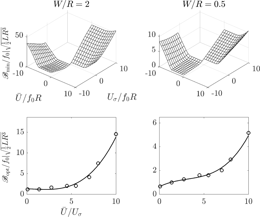
Figure 3: (top panels) A-priori bound (17) on the nonlinear growth of perturbations to unstable states of the class (5), minimized over all possible states states defined by (10) and (14). (bottom panels) Optimal bound obtained as a function of the basic flow’s stability parameter in the unstable range.

Nonlinear saturation bounds of the type above have been shown to exist even for systems subjected to forcing and dissipation [43]. Consider, for instance, the case of system (1b) with the $\bar{\xi}$-equation forced (damped?) by $R^{-2}[\bar{\psi},\hat{\psi}]$, where $\hat{\psi}$ is a prescribed function of latitude ($y$). This system is Lie–Poisson, with bracket as in (1b) and Hamiltonian given by $\smash{\hat{\mathcal{H}}=\mathcal{H}+R^{-2}\int\hat{\psi}\psi_{\sigma}}$. (In Holm, Luesink, and Pan [15], $\hat{\psi}$ is given the interpretation of a bottom (surface in the present case) topography; however, they do not include the corresponding topographic-$\beta$ term in the potential vorticity $\bar{\xi}$.) The system thus have the same Casimirs as the original (unforced, inviscid) system (1b), given in (3), and the $x$-translational symmetry of $\hat{\psi}$ makes the zonal momentum (4) to be conserved as well. Furthermore, (5) and (10) are admissible basic states, and all of the results above carry over mutatis mutandis to the forced case. (The only differences appear in the Casimir choices, with $\smash{C_{1}=-\frac{\bar{U}}{2R^{2}U_{\sigma}}\psi_{\sigma}^{2}-\frac{\hat{\psi}}{R^{2}}\psi_{\sigma}}$ and $C_{2}=0$ for the pseudoenergy–momentum (8) and $\smash{C_{1}=-\frac{\hat{\psi}}{R^{2}}\psi_{\sigma}-\frac{\bar{U}^{\mathscr{F}}}{R^{2}}\int^{\psi_{\sigma}}\mathscr{F}^{-1}(\psi_{\sigma})}$ and $C_{2}=0$ for that in (11).)

The above provides reason to expect (hope) that the bounds discussed here can play a role in arresting the growth of small-scale circulatory motions developing in direct numerical simulations of the IL⁰ system (1b), even in the forced–dissipative regime.

V Concluding remarks

The result of this work adds support to thermodynamically-active-layer ocean modeling as described by the IL⁰ system (1b), particularly for investigating with confidence in a geometric mechanics framework [15] the contribution of unresolved submesoscale motions to transport at resolvable scales in the upper ocean, a topic of active research [24]. Interestingly, the two-dimensional simulations described in Holm, Luesink, and Pan [15] suggest a scale separation consistent with satellite ocean color images and statistical analysis of in-situ Lagrangian ocean observations [9], but is challenged by three-dimensional surface-quasigeostrophic simulations [e.g., 18], which suggest a continuous inverse energy cascade. The extent to which the small-scale circulations and the associated scale separation represent a peculiarity of the IL⁰ model needs to be assessed, which is reserved for the future. An appropriate framework for this is provided by models with more vertical resolution, and hence better thermodynamics, than the IL⁰ model [37, 41, 7].

Supplementary material

This paper does not include supplementary material.

Author’s contributions

This paper is authored by a single individual who entirely carried out the work.

AIP Publishing data sharing policy

This paper does not involve the use of data.

Appendix A Free waves

For completeness, recall that the free waves of the IL⁰ model, i.e., infinitesimally small, normal-mode perturbations to a reference (i.e., quiescent) state of (1b) characterized by $\bar{\Psi}=0=\Psi_{\sigma}$, are given by [41]: a Rossby wave, with frequency $\smash{\omega=-\frac{k\beta}{|\mathbf{k}|^{2}+R^{-2}}}$ and for which $\delta\bar{\psi}\neq 0$ $\delta\psi_{\sigma}\neq 0$, and an $\omega=0$ mode, so-called force compensating mode [38], with $\delta\bar{\psi}=0=\delta\psi_{\sigma}$ or equivalently $2g_{\mathrm{b}}\delta h+H_{\mathrm{r}}\delta\vartheta=0$. Using the Casimir $\mathcal{C}=\smash{\frac{1}{2}R^{-2}\int\psi_{\sigma}^{2}}$, relative to this reference state, $\Delta(\mathcal{E}+\mathcal{C})=\smash{\frac{1}{2}\int|\nabla\delta\bar{\psi}|^{2}+R^{-2}(\delta\bar{\psi}^{2}+\delta\psi_{\sigma}^{2})=:\mathcal{E}_{\mathrm{f}}}$ is an exact invariant (which can called a free energy). Being positive-definite, it prevents the spontaneous growth of infinitesimal perturbations to the state with no currents. This result has received less attention than that pertaining to the most general reference state, characterized by $\bar{\Psi}=a=\mathrm{const}$. Upon choosing a Casimir of the form $\mathcal{C}=a\int R^{-2}\psi_{\sigma}+\bar{\xi}$, the following turns out to be a free energy relative to this reference state [39]: $\mathcal{E}_{\mathrm{f}}=\frac{1}{2}\delta^{2}(\mathcal{H}+C)=\smash{\frac{1}{2}\int|\nabla\delta\bar{\psi}|^{2}+R^{-2}\delta\bar{\psi}^{2}\equiv\frac{1}{2}\int|\delta\mathbf{u}|^{2}+f_{0}^{2}R^{2}\big{(}\frac{\delta h}{H_{\mathrm{r}}}+\frac{\delta\vartheta}{2g_{\mathrm{b}}}\big{)}^{2}}$. Note that this $\mathcal{E}_{\mathrm{f}}$ is positive-semidefinite, i.e., it can vanish for nonzero perturbations. More specifically, variations of $h$ and $\vartheta$ which leave $2g_{\mathrm{b}}h+H_{\mathrm{r}}\vartheta$ (for infinitesimal perturbations this is the force-compensating mode mentioned above) unaltered do not change $\mathcal{E}_{\mathrm{f}}$. Spontaneous growth of such variations cannot be prevented by $\mathcal{E}_{\mathrm{f}}$ conservation [37]. Yet formula (17) with $\bar{\mu}=0=\mu_{\sigma}$ provides an upper bound on their nonlinear growth.

Appendix B The axisymmetric basic state case

Ochoa, Sheinbaum, and Pavía [29] showed that unbounded $f$-plane, circular, solid-body-rotating, lens-like, outward-buoyancy-increasing, steady-vortex solutions to the primitive-equation set from which system (1b) derives (cold inhomogeneous so-called rodons) are formally stable. No steady-vortex solution to (1b) can be proved stable using the integrals of motion, given by (2), (3), and, instead of (4), $\smash{\mathcal{M}=-\int\sqrt{x^{2}+y^{2}}\bar{\xi}}$, which holds in the axisymmetric case. Indeed, only circular vortices with constant azimuthal velocity or, equivalently, local angular velocity inversely proportional to the radial position, which is physically odd, have a positive-definite pseudoenergy–momentum in an axisymmetric, bounded domain. In the limit when $R\to\infty$ or on the invariant subspace $\{\psi_{\sigma}=\mathrm{const}\}$ of system (1b), general axisymmetric basic flows can be shown to be Lyapunov stable using Arnold’s method (e.g., Ripa [34]).

References

- Anderson and McCreary [1985] Anderson, D.and McCreary, J., “On the role of the Indian Ocean in a coupled ocean-atmosphere model of El Niño and the Southern Oscillation,” J. Atmos. Sci. 42, 2439–2442 (1985).
- Arnold [1965] Arnold, V. I., “Conditions for nonlinear stability of stationary plane curvilinear flows of an ideal fluid,” Dokl. Akad. Nauk. SSSR 162, 975–978 (1965), engl. transl. Sov. Math. 6: 773-777 (1965).
- Arnold [1966] Arnold, V. I., “On an apriori estimate in the theory of hydrodynamical stability,” Izv. Vyssh. Uchebn. Zaved Mat. 54, 3–5 (1966), engl. transl. Am. Math. Soc. Transl. Ser. 2 79: 267-269 (1969).
- Beier [1997] Beier, E., “A numerical investigation of the annual variability in the Gulf of California,” J. Phys. Oceanogr. 27, 615–632 (1997).
- Benilov [1993] Benilov, E., “Baroclinic instability of large-amplitude geostrophic flows,” J. Fluid Mech. 251, 501–514 (1993).
- Benjamin [1984] Benjamin, T., “Impulse, flow force and variational principles,” IMA J. Appl. Math. 32, 3–68 (1984).
- Beron-Vera [2020] Beron-Vera, F. J., “Multilayer shallow-water model with stratification and shear,” Rev. Mex. Fís., in press (arXiv:physics/0312083) (2020).
- Beron-Vera et al. [2008] Beron-Vera, F. J., Brown, M. G., Olascoaga, M. J., Rypina, I. I., Koçak, H., and Udovydchenkov, I. A., “Zonal jets as transport barriers in planetary atmospheres,” J. Atmos. Sci. 65, 3316–3326 (2008).
- Beron-Vera and LaCasce [2016] Beron-Vera, F. J.and LaCasce, J. H., “Statistics of simulated and observed pair separations in the gulf of mexico,” J. Phys. Oceanorg 46, 2183–2199 (2016).
- Beron-Vera and Ripa [1997] Beron-Vera, F. J.and Ripa, P., “Free boundary effects on baroclinic instability,” J. Fluid Mech. 352, 245–264 (1997).
- Cotter et al. [2020] Cotter, C., Crisan, D., Holm, D., Pan, W., and Shevchenko, I., “Data assimilation for a quasi-geostrophic model with circulation-preserving stochastic transport noise,” J. Stat. Phys. 179, 1186 – 1221 (2020).
- Fukamachi, McCreary, and Proehl [1995] Fukamachi, Y., McCreary, J. P., and Proehl, J. A., “Instability of density fronts in layer and continuously stratified models,” J. Geophys. Res. 100, 2559–2577 (1995).
- Gouzien et al. [2017] Gouzien, E., Lahaye, N., Zeitlin, V., and Dubos, T., “Thermal instability in rotating shallow water with horizontal temperature/density gradients,” Physics of Fluids 29, 101702 (2017).
- Holm [2015] Holm, D. D., “Variational principles for stochastic fluid dynamics,” Proceedings of the Royal Society A: Mathematical, Physical and Engineering Sciences 471, 20140963 (2015).
- Holm, Luesink, and Pan [2020] Holm, D. D., Luesink, E., and Pan, W., “Stochastic mesoscale circulation dynamics in the thermal ocean,” arXiv:2006.05707 (2020).
- Holm, Marsden, and Ratiu [1998] Holm, D. D., Marsden, J. E., and Ratiu, T., “The Euler-Poincaré equations and semidirect products with applications to continuum theories,” Adv. in Math. 137, 1–81 (1998).
- Holm et al. [1985] Holm, D. D., Marsden, J. E., Ratiu, T., and Weinstein, A., “Nonlinear stability of fluid and plasma equilibria,” Phys. Rep. 123, 1–116 (1985).
- Klein et al. [2008] Klein, P., Hua, B. L., Lapeyre, G., Capet, X., Le Gentil, S., and Sasaki, H., “Upper ocean turbulence from high-resolution 3D simulations,” J. Phys. Oceanogr. 38, 1748–1763 (2008).
- Kurganov, Liu, and Zeitlin [2020] Kurganov, A., Liu, Y., and Zeitlin, V., “Moist-convective thermal rotating shallow water model,” Physics of Fluids 32, 066601 (2020), https://doi.org/10.1063/5.0007757 .
- Lahaye, Zeitlin, and Dubos [2020] Lahaye, N., Zeitlin, V., and Dubos, T., “Coherent dipoles in a mixed layer with variable buoyancy: Theory compared to observations,” Ocean Modelling 153, 101673 (2020).
- Lavoie [1972] Lavoie, R., “A mesoscale numerical model of lake-effect storms,” J. Atmos. Sci. 29, 1025 – 1040 (1972).
- McCreary, Zhang, and Shetye [1997] McCreary, J. P., Zhang, S., and Shetye, S. R., “Coastal circulations driven by river outflow in a variable-density 1 -layer model,” J. Geophys. Res. 102, 15,535–15,554 (1997).
- McIntyre and Shepherd [1987] McIntyre, M.and Shepherd, T., “An exact local conservation theorem for finite-amplitude disturbances to non-parallel shear flows, with remarks on Hamiltonian structure and on Arnol’d’s stability theorems,” J. Fluid Mech. 181, 527–565 (1987).
- McWilliams [2016] McWilliams, J. C., “Submesoscale currents in the ocean,” Proc R Soc A 472, 20160117 (2016).
- Moreles et al. [2021] Moreles, E., Zavala-Hidalgo, J., Martinez-Lopez, B., and Ruiz-Angulo, A., “Influence of stratification and Yucatan Current transport on the Loop Current Eddy shedding process,” Journal of Geophysical Research: Oceans 126, e2020JC016315 (2021).
- Morrison [1998] Morrison, P. J., “Hamiltonian description of the ideal fluid,” Rev. Mod. Phys. 70, 467–521 (1998).
- Morrison and Hazeltine [1984] Morrison, P. J.and Hazeltine, R. D., “Hamiltonian formulation of reduced magnetohydrodynamics,” Phys. Fluids 27, 886–897 (1984).
- O’Brien and Reid [1967] O’Brien, J. J.and Reid, R. O., “The non-linear response of a two-layer, baroclinic ocean to a stationary, axially-symmetric hurricane: Part I: Upwelling induced by momentum transfer,” J. Atmos. Sci. 24, 197–207 (1967).