Random Shadows and Highlights:
A new data augmentation method for Extreme Lighting Conditions

Abstract

In this paper, we propose a new data augmentation method, Random Shadows and Highlights (RSH) to acquire robustness against lighting perturbations. Our method creates random shadows and highlights on images, thus challenging the neural network during the learning process such that it acquires immunity against such input corruptions in real world applications. It is a parameter-learning free method which can be integrated into most vision related learning applications effortlessly. With extensive experimentation, we demonstrate that RSH not only increases the robustness of the models against lighting perturbations, but also reduces over-fitting significantly. Thus RSH should be considered essential for all vision related learning systems. Code is available at: https://github.com/OsamaMazhar/Random-Shadows-Highlights.

Index Terms—  Robotic vision, Harsh conditions, Generalization, Data augmentation, Convolutional Neural Networks

1 Introduction

It is often claimed that the performance of deep learning algorithms have attained super-human capabilities. However, real-world effectiveness of deep learning computer vision algorithms often fail to match the published performance on benchmarks [1]. The vision models are largely fragile and do not generalize across realistic unconstrained scenarios [2], e.g., when they encounter instances of classes, textures, or environmental conditions that were not covered by the training data [3]. This could have serious consequences where the failures could lead to potentially catastrophic results as in the case of self-driving vehicles.

The authors of [4] studied the existing hypotheses concerning the methods to improve the robustness of the deep networks. Of particular relevance to our work, the technique of perturbing data without altering class labels, also known as data augmentation, has been proven to greatly improve model robustness and generalization performance [5, 6]. It artificially inflates a dataset through label-preserving transforms to derive new samples from the originals. Data augmentation offers straightforward strategies to learn invariances that are challenging to encode architecturally. The most prevalent forms of data augmentation methodologies rely mostly on hand crafted features or include geometric distortions such as random cropping, zooming, rotation and flipping [7]. Other methods include color space transformation, linear intensity scaling and elastic deformation. These methods are successful at teaching mainly orientation and scale invariance, but are insufficient for other practical cases like occlusion, texture and complex illumination variations. This is however often achieved by domain randomization on rendered images in simulation for Sim2Real transfer [8].

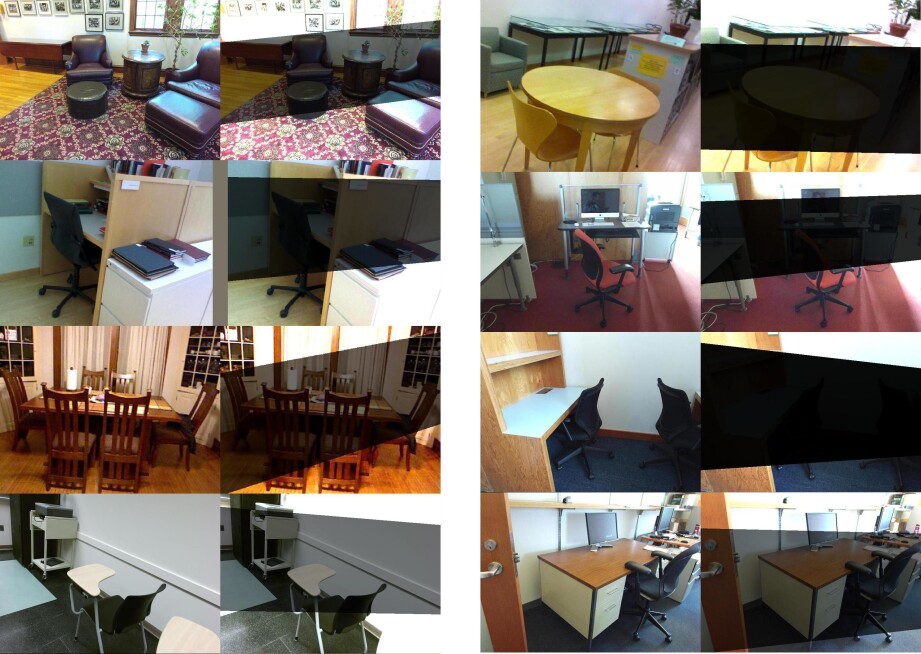
Fig. 1: Samples of our proposed Random Shadows and Highlights (RSH) data augmentation scheme.

Extreme lighting conditions such as dark shadows, intense highlights or change in brightness substantially affect the performance of deep models in image classification or object detection tasks. To address such illumination variations and bridging the reality gap, this paper introduces a new data augmentation methodology, Random Shadows and Highlights (RSH) for real camera images. The proposed strategy mimics high-contrast extreme lighting conditions by creating random shadows and highlights in the images. RSH is a parameter-learning free lightweight method which can be integrated with most vision related learning models without the need to change the learning strategy. The proposed data augmentation method is utilized to imitate the limitations of conventional RGB sensors to handle extreme light conditions.

2 Related Works

Data augmentation is a strategy that aims to improve robustness of the models to unforeseen data shifts which they might encounter in real-world. It explicitly teaches invariance to whichever transformation is used on the dataset. For example, robustness against occlusions can be learned through Cutout [9] and Random Erasing [10]. Cutout randomly masks out square regions of input to generate new images to simulate occluded examples. Random Erasing additionally varies size and aspect ratio of the masked region. It also allows to replace pixel values with random noise. Instead of occluding an image, CutMix [11] substitutes a portion of image with a portion of another image while the ground truth labels are also mixed proportionally to the area of the patches. Mixup [12] is a another regularization strategy that produces elementwise convex combination of two images. AugMix [13] mixes together the results of several shorter augmentation chains in convex combinations to prevent image degradation while maintaining augmentation diversity. Alpha-blending two images generate pixel-level features that a camera might never produce and that could potentially affect model performance. To prevent this, RICAP [14] spatially blend four cropped images to create a new image. It performs occupancy estimation instead of classification, by mixing the four class labels with ratios proportional to the areas of the cropped images. The method proposed in [15] is closest to our proposed strategy. Nevertheless, they only create illumination circles on the images which does not represent the real world lighting perturbations often seen in indoor environments or even outdoors caused by shadows of the buildings. Separate from hand-crafted methodologies are learned augmentation methods such as AutoAugment [16], patch Gaussian augmentation [6], learned image transformations [5] and DeepAugment [4].

3 DATASETS

For image classification, we evaluate RSH on Tiny-ImageNet [17], CIFAR-10 and CIFAR-100 [18]. Tiny-ImageNet is a miniature version of the ImageNet dataset with 200 classes. Each class contains 500 training and 50 validation images yielding 100,000 training and 10,000 validation samples. All images are of size $64\times 64\times 3$. CIFAR-10 consists of 60,000 colour images in 10 classes with images of objects like airplanes, birds, trucks, etc. Each class consists of 6,000 images. The training set contains 50,000 images while 10,000 images are in the validation set. CIFAR-100 is similar to CIFAR-10 except that it has 100 classes with 600 images in each class. Each image comes with a fine and a coarse label. For object detection, we utilize the PASCAL VOC 2007 dataset [19] which provides 9,963 images of realistic scenes containing 24,640 annotated objects. The dataset is split into 50% for training/validation and 50% for testing. There are 20 classes of objects which are almost equally distributed in the images.

4 OUR APPROACH

Shadows cast by buildings in outdoors often take the form of trapezoids. Furthermore, luminous light entering through windows or doors inside the buildings also take similar shapes. We devise an algorithm to create Random Shadows and Highlights on images imitating trapezoidal shape with its base aligned with the vertical axis of the image.

Input: Input image ${I}$;

         Image size ${W}$, ${H}$ and $c$;

         RSH probability ${p}$;

         Highlights range ${H_{l}}$, ${H_{h}}$;

         Shadows range ${S_{l}}$, ${S_{h}}$;

         Left edge ranges ${l_{ul}}$, ${l_{uh}}$ and ${l_{ll}}$, ${l_{lh}}$;

         Right edge ranges ${r_{ul}}$, ${r_{uh}}$ and ${r_{ll}}$, ${r_{lh}}$.

Output: Transformed image $I^{*}$

Initialization: $p_{1}\leftarrow\text{Rand}(0,1).$

1 if $p_{1}\geq p$ then

2       $I^{*}\leftarrow I$;

3       return $I^{*}$.

4else

5       $L_{lf}\leftarrow\text{Rand}(l_{ll},l_{lh})\times H;$

6       $L_{hf}\leftarrow\text{Rand}(l_{ul},l_{uh})\times H;$

7       $R_{lf}\leftarrow\text{Rand}(r_{ll},r_{lh})\times H;$

8       $R_{hf}\leftarrow\text{Rand}(r_{ul},r_{uh})\times H;$

9       $P_{bl}\leftarrow(0,L_{lf}+L_{hf});$

10       $P_{tl}\leftarrow(0,L_{hf});$

11       $P_{br}\leftarrow(W,R_{lf}+R_{hf});$

12       $P_{tr}\leftarrow(W,R_{hf});$

13       $I_{mask}\leftarrow\text{ContourFill}(\text{Zeros}(H,W,c),[P_{tl},P_{tr},P_{br},P_{bl}])$;

14       $I_{inv\_mask}\leftarrow\neg I_{mask}$;

15       $S_{f}\leftarrow\text{Rand}(S_{l},S_{h})$;

16       $H_{f}\leftarrow\text{Rand}(H_{l},H_{h})$;

17       $I_{shadow}\leftarrow\text{adjustBrightness}(I,S_{f})$;

18       $I_{high}\leftarrow\text{adjustBrightness}(I,H_{f})$;

19       $I^{*}\leftarrow I_{shadow}(I_{mask})+I_{high}(I_{inv\_mask})$;

20       return $I^{*}.$

21 end if

Algorithm 1 Random Shadows and Highlights

For an image ${I}$, Random Shadows and Highlights is applied with a probability $p$ in training. For probability $1-p$, the image is left unchanged. RSH is driven by twelve input parameters to create random shadows and highlights. These variables include highlights range $H_{l}$, $H_{h}$ and shadows range $S_{l}$, $S_{h}$. These also include left edge ranges $l_{ul}$, $l_{uh}$ and $l_{ll}$, $l_{lh}$, and right edge ranges $r_{ul}$, $r_{uh}$ and $r_{ll}$, $r_{lh}$, to randomly obtain four points in total i.e., two on each vertical axis of the image which are subsequently employed to draw a trapezoid. For an input image of size $W\times H$, our algorithm randomly creates a contour on the image driven by the provided parameters ranges. The brightness of the pixels inside the contour is reduced by a factor $S_{f}$ which is randomly chosen within the predefined range $S_{l}$ and $S_{h}$. Similarly, the brightness of the pixels outside the contour is increased by a factor $H_{f}$ obtained from within $H_{l}$ and $H_{h}$. The detailed procedure of creating the contour mask(s) and ultimately creating an image with shadows and highlights is shown in Alg 1.

5 EXPERIMENTS

5.1 Image Classification

Through extensive experimentation, we study the impact of Random Shadows and Highlights (RSH) in comparison to a set of related augmentations methods. Among the commonly employed strategies, the most relevant ones to our work are Gamma Correction and Color Jitter. Varying powers of gamma darkens or lightens the shadows in the image. While in Color Jitter, we randomly change the brightness, contrast, saturation and hue of the image. Moreover, we also compare our results with the method proposed in [15], we call it Disk Illumination. To study over-fitting, we quantify the Train-Test Difference (TTD), as the name suggests, difference in error on the train set and test set, with and without RSH perturbations. When lighting corruption is applied to the test set, its probability is set to $1$. The RSH parameters which were chosen in our experiments are: $H_{l}=1$, $H_{h}=2$, $S_{l}=0$, $S_{h}=1$, $l_{ul}$ and $r_{ul}=0$, $l_{uh}$ and $r_{uh}=0.3$, $l_{ll}$ and $r_{ll}=0.4$, $l_{lh}$ and $r_{lh}=0.8$. Gamma is randomly changed from $0$ to $1.5$ while brightness, contrast and saturation ranges are $0$ to $2$, and hue changes from $-0.5$ to $0.5$ randomly.

Architectures: We adopted two architectures on Tiny-ImageNet, CIFAR-10 and CIFAR 100: EfficientNet [20] and AlexNet [21]. More precisely, we employed the EfficientNet-B0 architecture. The models are pre-trained on the ImageNet dataset except the SoftMax layer which is adopted for each dataset and initialized with random weights. The training is performed only for $20$ epochs at a learning rate of $1e^{-3}$ and a momentum of $0.9$ with the SGD optimizer.

Method	Train Error	Test Error	Test Error RSH (1)	TTD w/o RSH	TTD RSH (1)
Baseline	0.303	0.408	0.630	0.105	0.327
RGC (0.5)	0.301	0.396	0.603	0.095	0.302
RCJ (0.5)	0.415	0.406	0.612	$-$0.009	0.197
RDI (0.5)	0.493	0.410	0.627	$-$0.083	0.134
RSH (0.5)	0.353	0.407	0.449	0.054	0.096
RGC (1)	0.323	0.400	0.600	0.077	0.277
RCJ (1)	0.485	0.459	0.656	$-$0.026	0.171
RDI (1)	0.639	0.631	0.780	$-$0.008	0.141
RSH (1)	0.411	0.434	0.450	0.023	0.039

Table 1: Performance evaluation of EfficientNet-B0 on TinyImageNet. For comparison, models are trained with Random Gamma Correction (RGC), Random Color Jitter (RCJ) and Random Disk Illumination (RDI) as well. Apart from train and test error computation, performance is measured with lighting perturbations as well by applying RSH in the test set with $p=1$. Moreover, the Train-Test Difference (TTD) is also computed to quantify over-fitting of the models. Negative TTD implies over-regularization which is not desired.

5.1.1 Classification Evaluation

The performances of the selected data augmentation strategies are evaluated at different activation probabilities $p$, ranging from $0.0$ to $1.0$ with a step size of $0.1$. Table 1 presents the results of these experiments at $p=0.5$ and $p=1$ only. At a first glance, it may appear that the performance with RSH decreases slightly on test sets when no lighting perturbations are applied. To some extent, this is true and is justified by the observations made in [22] that argues that standard accuracy is often compromised to obtain robust models. However, when tested with lighting corruptions, our strategy out-scores all other methods with a considerable margin by obtaining least test errors at both probabilities. In fact, Figure 2 illustrates that RSH is extremely robust against lighting perturbations at all values of $p$. Table 1, also shows that for lighting perturbations at $p=1$ on the test set, the performance of the model trained with RSH is increased by approximately 25% at both $p=0.5$ and $p=1$ when compared to RGC which performed best among other strategies. Furthermore, we estimate the Train-Test Difference (TTD) to measure over-fitting for cases with and without lighting corruption. In addition to the increased robustness, our RSH augmentation method proves to have reduced over-fitting significantly as well.

Impact of hyperparameters:

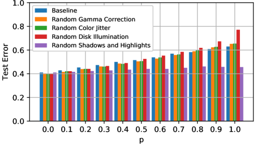
Fig. 2: Test error comparison between different data augmentation strategies for different levels of lighting perturbations. p represents data augmentation activation probabilities for each individual technique in training as well as that of lighting perturbations in test set.

We also conduct experiments to study the impact of RSH hyperparameters on the model performance. Figure 3 illustrates the results obtained when training AlexNet on CIFAR-10 with increasing RSH probability from $0.0$ to $1.0$. The probability of lighting corruption is set to 1 in the test set. It is evident, that the model overfits severely when no RSH augmentation is applied during training. Nevertheless, RSH $p$ increases in the training, robustness of the network increases continuously until we obtain almost the same train-test prediction accuracy, which is desired in most cases.

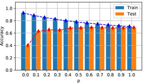
Fig. 3: Performance evaluation on CIFAR-10 when trained with different activation probabilities of RSH. The probability of lighting corruptions is set to $1$ for all values of $p$. It is evident that with the increase in $p$, over-fitting decreases continuously until the model fits almost perfectly for both train and test sets.

Fig. 4: Impact of changing $H$ and $S$ hyperparameters. For all cases we set $H_{h}=2$ while $S_{l}=0$. The X axis represents increasing span of choice for highlights and shadows. Clearly, with wider range, RSH performs best in terms of accuracy.

We also evaluate the impact of changing other hyperparameters. Figure 4 illustrates that increasing the range of highlights and shadows improves not only the accuracy of the model, but enhances the TTD by 3.125% as well. The significance of the “shadows area” is also assessed on CIFAR-100 by changing the values of $l_{lh},r_{lh},l_{ul}$ and $r_{ul}$ while keeping $l_{ll},r_{ll},l_{uh}$ and $r_{uh}$ constant. A marginal improvement of 1.7% is observed with the values presented in Section 5.1 as compared to the the least performing ones.

5.2 Object Detection

In our experiments for object detection, we employ a single-stage end-to-end object detector DETR proposed in [23]. It is among the pioneering works that exploited transformers in the image domain. However, DETR technically is still a combination of CNN and self-attention. We utilize ResNet-50 as the backbone features extractor while the object detector head is adopted to suit the number of classes in the Pascal VOC 2007 dataset. The weights are initialized from a checkpoint pretrained on the COCO object dataset. Thus, the hyperparameters of the transformer in DETR are set to default with $6$ encoder and decoder layers, $8$ attention heads, and $100$ number of queries. The learning rate for both backbone and transformer layers is set to $8\times 10^{-6}$ while training is terminated after $150$ epochs for each experiment. We perform experiments with and without Random Shadows and Highlights augmentation on the Pascal VOC 2007 dataset.

Model	mAP@IoU=0.5			TTD w/o RSH	TTD w/ RSH (1)
	Train	Test	Test w/ RSH (1)
Baseline	0.888	0.751	0.639	0.137	0.249
RSH (1)	0.872	0.751	0.705	0.121	0.167

Table 2: Performance evaluation of our RSH augmentation strategy for object detection on the Pascal VOC 2007 dataset.

5.2.1 Detection Evaluation

The performance evaluation of DETR with RSH on the Pascal VOC 2007 dataset is presented in Table 2. For each setting, mean of 20 evaluation trials is computed. It is evident from the results that the model trained with our RSH augmentation not only maintained its standard accuracy but also improved the robustness against lighting corruption by 10.328% compared to the baseline. Clear improvements in TTD with and without RSH perturbations in the test set can also be seen.

6 CONCLUSION

A new lightweight learning-free data augmentation strategy is presented in this paper to acquire robustness against lighting corruption. This is achieved by creating random shadows and highlights on the images during training. The models trained with the proposed augmentation method not only out-scored other similar methods against lighting perturbations but also reduced over-fitting on the training data significantly. The results in the performed experiments demonstrate that RSH should be considered essential in CNN model training. In the future, we plan to apply our method on other applications, e.g, facial recognition and person re-identification.

References

- [1] N. Sünderhauf, O. Brock, W. Scheirer, R. Hadsell, D. Fox, J. Leitner, B. Upcroft, P. Abbeel, W. Burgard, M. Milford, et al., “The limits and potentials of deep learning for robotics,” The Intl. Journal of Robotics Research, vol. 37, no. 4-5, pp. 405–420, 2018.
- [2] D. Yin, R. Gontijo Lopes, Jon S., Ekin D. C., and J. Gilmer, “A Fourier perspective on model robustness in computer vision,” in Advances in Neural Information Processing Systems, 2019, pp. 13276–13286.
- [3] M. Bijelic, T. Gruber, F. Mannan, F. Kraus, W. Ritter, K. Dietmayer, and F. Heide, “Seeing through fog without seeing fog: Deep multimodal sensor fusion in unseen adverse weather,” in Proc. of the IEEE/CVF Conf. on Computer Vision and Pattern Recognition, 2020, pp. 11682–11692.
- [4] D. Hendrycks, S. Basart, N. Mu, S. Kadavath, F. Wang, E. Dorundo, R. Desai, T. Zhu, S. Parajuli, M. Guo, et al., “The many faces of robustness: A critical analysis of out-of-distribution generalization,” arXiv preprint arXiv:2006.16241, 2020.
- [5] B. Zoph, E. D. Cubuk, G. Ghiasi, T. Lin, J. Shlens, and Q. V. Le, “Learning data augmentation strategies for object detection,” in European Conf. on Computer Vision. Springer, 2020, pp. 566–583.
- [6] R. G. Lopes, D. Yin, B. Poole, J. Gilmer, and E. D. Cubuk, “Improving robustness without sacrificing accuracy with patch Gaussian augmentation,” arXiv preprint arXiv:1906.02611, 2019.
- [7] K. He, X. Zhang, S. Ren, and J. Sun, “Deep residual learning for image recognition,” in Proc. of the IEEE Conf. on Computer Vision and Pattern Recognition, 2016, pp. 770–778.
- [8] J. Tobin, R. Fong, A. Ray, J. Schneider, W. Zaremba, and P. Abbeel, “Domain randomization for transferring deep neural networks from simulation to the real world,” in 2017 IEEE/RSJ Intl. Conf. on Intelligent Robots and Systems (IROS). IEEE, 2017, pp. 23–30.
- [9] T. DeVries and G. W Taylor, “Improved regularization of convolutional neural networks with cutout,” arXiv preprint arXiv:1708.04552, 2017.
- [10] Z. Zhong, L. Zheng, G. Kang, S. Li, and Y. Yang, “Random erasing data augmentation,” Proc. of the AAAI Conf. on Artificial Intelligence, vol. 34, no. 07, pp. 13001–13008, Apr. 2020.
- [11] S. Yun, D. Han, S. J. Oh, S. Chun, J. Choe, and Y. Yoo, “CutMix: Regularization strategy to train strong classifiers with localizable features,” in Proc. of the IEEE Intl. Conf. on Computer Vision, 2019, pp. 6023–6032.
- [12] H. Zhang, M. Cisse, Y. N. Dauphin, and D. Lopez-Paz, “mixup: Beyond empirical risk minimization,” arXiv preprint arXiv:1710.09412, 2017.
- [13] D. Hendrycks, N. Mu, E. D. Cubuk, B. Zoph, J. Gilmer, and B. Lakshminarayanan, “Augmix: A simple data processing method to improve robustness and uncertainty,” arXiv preprint arXiv:1912.02781, 2019.
- [14] R. Takahashi, T. Matsubara, and K. Uehara, “Data augmentation using random image cropping and patching for deep CNNs,” IEEE Trans. on Circuits and Systems for Video Technology, 2019.
- [15] D. Sakkos, H. P. Shum, and E. S. Ho, “Illumination-based data augmentation for robust background subtraction,” in 13th Intl. Conf. on Software, Knowledge, Information Management and Applications (SKIMA). IEEE, 2019, pp. 1–8.
- [16] E. D. Cubuk, B. Zoph, D. Mane, V. Vasudevan, and Q. V. Le, “AutoAugment: Learning augmentation policies from data,” arXiv preprint arXiv:1805.09501, 2018.
- [17] Y. Le and X. Yang, “Tiny ImageNet Visual Recognition Challenge,” https://tiny-imagenet.herokuapp.com/, 2015.
- [18] A. Krizhevsky et al., “Learning multiple layers of features from tiny images,” Tech Report, 2009.
- [19] M. Everingham, L. Van Gool, C. K. I. Williams, J. Winn, and A. Zisserman, “The PASCAL Visual Object Classes Challenge 2007 (VOC2007) Results,” http://www.pascal-network.org/challenges/VOC/voc2007/workshop/index.html.
- [20] M. Tan and Q. V. Le, “EfficientNet: Rethinking model scaling for convolutional neural networks,” arXiv preprint arXiv:1905.11946, 2019.
- [21] A. Krizhevsky, I. Sutskever, and G. E. Hinton, “ImageNet classification with deep convolutional neural networks,” Communications of the ACM, vol. 60, no. 6, pp. 84–90, 2017.
- [22] D. Tsipras, S. Santurkar, L. Engstrom, A. Turner, and A. Madry, “Robustness may be at odds with accuracy,” arXiv preprint arXiv:1805.12152, 2018.
- [23] N. Carion, F. Massa, G. Synnaeve, N. Usunier, A. Kirillov, and S. Zagoruyko, “End-to-end object detection with transformers,” arXiv preprint arXiv:2005.12872, 2020.