Uniform Error and Posterior Variance Bounds for Gaussian Process Regression with Application to Safe Control
Abstract
In application areas where data generation is expensive, Gaussian processes are a preferred supervised learning model due to their high data-efficiency. Particularly in model-based control, Gaussian processes allow the derivation of performance guarantees using probabilistic model error bounds. To make these approaches applicable in practice, two open challenges must be solved i) Existing error bounds rely on prior knowledge, which might not be available for many real-world tasks. (ii) The relationship between training data and the posterior variance, which mainly drives the error bound, is not well understood and prevents the asymptotic analysis. This article addresses these issues by presenting a novel uniform error bound using Lipschitz continuity and an analysis of the posterior variance function for a large class of kernels. Additionally, we show how these results can be used to guarantee safe control of an unknown dynamical system and provide numerical illustration examples.
Keywords: Gaussian processes, uniform error bounds, posterior variance analysis, safe control, learning in feedback systems
1 Introduction
Modeling nonlinear systems using supervised learning techniques (Nørgård et al., 2000) enabled model-based control to succeed in highly complex tasks, such as controlling a robotic unicycle in simulation (Deisenroth et al., 2013). Nevertheless, the application of learning-based control in real-world safety-critical scenarios, like autonomous driving, assistive and rehabilitation robotics, or personalized disease treatment is rare, due to missing performance guarantees for the resulting closed-loop behavior. Empirical evaluations exist, e.g., (Huval et al., 2015) for autonomous cars, but are insufficient if the physical integrity of systems is at risk. As in human-centric applications training data is expensive to acquire, Gaussian processes (GPs) are particularly appealing as the regression generalizes well for small training sets. Furthermore, GPs are a probabilistic method based on Bayesian principles (Rasmussen and Williams, 2006), which allows to properly encode prior knowledge and to quantify the uncertainty in the model.
Due to these properties, GPs gained increasing attention in the field of reinforcement learning and system identification. Especially, when safety guarantees are necessary, GPs are favored in reinforcement learning (Berkenkamp et al., 2016a, c, 2017; Koller et al., 2018) as well as control (Berkenkamp and Schoellig, 2015; Umlauft et al., 2017; Beckers and Hirche, 2018; Lederer et al., 2020; Umlauft et al., 2018; Helwa et al., 2019). These approaches heavily rely on error bounds of GP regression and are therefore limited by the strict assumptions made in previous works on GP uniform error bounds (Srinivas et al., 2012; Chowdhury and Gopalan, 2017).
Furthermore, these bounds are based on the posterior variance function whose behavior for an increasing number of training data is not well understood. Especially when data points are added on-line, e.g. during the control tasks, compare (Umlauft and Hirche, 2020), the posterior variance has barely been analyzed formally due to a lack of suitable bounds. Generally, there is only limited understanding of the interaction between learning and control in feedback systems, which is crucial to provide guarantees for the control error and mainly motivates the work in this article.
1.1 Contribution
The main contribution of this article is the derivation of a novel uniform error bound for GPs, which is guaranteed to converge to in the limit of infinitely many, suitably distributed training samples, and allows safety guarantees for the control of unknown dynamical systems. For the derivation of this uniform error bound, we proceed as follows: First, we derive a bound for the posterior variance of GPs with Lipschitz continuous kernels and propose improvements for a more specific class of kernels. Additionally, we derive sufficient conditions for the distribution of the data to ensure the convergence of our bound to zero. Second, we present a uniform error bound for GPs, which requires less prior knowledge and assumptions than in prior work as it is based on Lipschitz continuity. This uniform error bound is based on preliminary work presented in (Lederer et al., 2019). We analyze bounds for the derivatives of GP sample functions and employ them as constraints in likelihood maximization in order to ensure that the prior distribution fits to the available knowledge of the unknown function. Furthermore, we use the bounds on sample functions and the posterior variance to investigate the asymptotic behavior of the uniform error bound, which shows that arbitrarily small error bounds can be achieved under weak assumptions on the training data. The proposed GP bounds are employed to derive safety guarantees for controlling unknown dynamical systems based on Lyapunov theory (Khalil, 2002). We illustrate all our results in simulations and demonstrate the superiority of our bounds for the GP posterior variance compared to state-of-the-art methods. Finally, we demonstrate the safety of our control approach in an experiment with a robotic manipulator.
1.2 Structure of this article
This article is structured as follows: We briefly introduce Gaussian process regression and provide a in-depth discussion of the related work in Section 2. An analysis of the posterior variance bound is presented in Section 3, followed by the derivation of a uniform error bound for GPs in Section 4 using the probabilistic Lipschitz constant. In Section 5 we demonstrate how the results of the former two section can be employed to prove safety of a model-based control law. A numerical illustration and comparison to prior work are provided in Section 6, followed by a conclusion in Section 7.
1.3 Notation
Vectors/matrices are denoted by lower/upper case bold symbols, the identity matrix by , the Euclidean norm by , and and the minimum and maximum eigenvalues of a matrix , respectively. Sets are denoted by upper case black board bold letters, and sets restricted to positive/non-negative numbers have an indexed /, e.g. for all positive real valued numbers. The cardinality of sets is denoted by and subsets/strict subsets are indicated by . The expectation operator can have an additional index to specify the considered random variable. Class notation is used to provide asymptotic upper bounds on functions. Similarly, we use class functions , which are strictly increasing, and satisfy . The ceil and floor operator are denoted by and , respectively.
2 Related Work and Background
2.1 Gaussian Process Regression
A Gaussian process is a stochastic process such that any finite number of outputs is assigned a joint Gaussian distribution with prior mean function and covariance defined through the kernel (Rasmussen and Williams, 2006). Therefore, the training outputs can be considered as observations of a sample function of the GP distribution perturbed by i.i.d. zero mean Gaussian noise with variance . Without any specific information about the unknown function such as an approximate model, the prior mean function is typically set to . We also assume this in the following without loss of generality. Regression is performed by conditioning the prior GP distribution on the training data and a test point . The conditional posterior distribution is again Gaussian and can be calculated analytically. For this reason, we define the kernel matrix and the kernel vector through and , respectively, with . Then, the posterior mean and variance are given by
| (1) | ||||
| (2) |
where denotes the data covariance matrix and .
The kernel typically depends on so called hyperparameters which allow to shape the prior distribution without changing properties of the sample functions such as periodicity or stationarity. Although there is a variety of methods available for hyperparameter tuning (Rasmussen and Williams, 2006), in control-oriented applications they are often fitted to the training data by maximizing the marginal log-likelihood , which is commonly performed using gradient-based optimization methods.
2.2 Posterior Variance Bounds of Gaussian Processes
Posterior variance bounds are well known for many methods closely related to Gaussian process regression. For noise-free interpolation, the posterior variance has been analyzed using spectral methods (Stein, 1999). While the asymptotic behavior can be analyzed efficiently with such methods, they are not suited to bound the posterior variance for specific training data sets. In the context of noise-free interpolation, many bounds from the area of scattered data approximation can be applied due to the equivalence of the posterior variance and the power function (Kanagawa et al., 2018). Therefore, classical results (Wu and Schaback, 1993; Wendland, 2004; Schaback and Wendland, 2006) as well as newer findings (Beatson et al., 2010; Scheuerer et al., 2013) can be directly used for GP interpolation. However, it is typically not clear how these results can be generalized to regression with noisy observations.
Posterior variance bounds for GP regression have mostly been developed as intermediate results for more complex problems. For example, a variance bound has been developed for GPs with isotropic kernels in the context of Bayesian optimization (Shekhar and Javidi, 2018) while bounds for general kernels have been investigated within the analysis of average learning curves (Opper and Vivarelli, 1999; Williams and Vivarelli, 2000) and experimental design (Wang and Haaland, 2018). Although these bounds are well-suited for low data regimes, they fail to capture the asymptotic behavior. Therefore, upper bounds on the posterior variance are missing which allow to describe the learning behavior over the whole range of training data densities.
2.3 Error Bounds of Gaussian Process Regression
Uniform error bounds play a crucial role in quantifying the precision of a function approximator. For the case of noise free data, results of scattered data approximation with radial basis functions can be applied to derive such bounds (Wendland, 2004) and translate to GP regression with stationary kernels. Using Fourier transform methods, the classical result in (Wu and Schaback, 1993) derives error bounds for functions in the reproducing kernel Hilbert space (RKHS) associated with the interpolation kernel. By utilizing further properties of the RKHS, a uniform error bound with increased convergence rate is derived in (Schaback, 2002). These bounds are driven by the power function, which are - under certain conditions - equivalent to the GP posterior standard deviation (Kanagawa et al., 2018).
Extending scattered data interpolation to noisy observations leads to the concept of regularized kernel regression (Kanagawa et al., 2018). For squared cost functions, this kernel ridge regression is identical to the GP posterior mean function (Rasmussen and Williams, 2006). The corresponding error bounds, e.g., in (Mendelson, 2002) depend on the empirical covering number and the norm of the unknown function in the associated RKHS. With empirical covering numbers, tighter error bounds can be derived under mild assumptions (Shi, 2013). For general regularization, error bounds are derived in (Dicker et al., 2017) as a function of the regularization and the RKHS norm of the function.
Uniform error bounds depending on the maximum information gain and the RKHS norm for GP regression were derived in (Srinivas et al., 2012). However, these results only apply to bounded sub-Gaussian observation noise, which is a limitation compared to regularized kernel regression. To analyze the regret of an upper confidence bound algorithm in multi-armed bandit setting, an improved bound is derived in (Chowdhury and Gopalan, 2017). Although these bounds are widely applied in safe reinforcement learning and control, they suffer from the following drawbacks: i) They depend on constants which are very difficult to calculate, which is no problem for the theoretical analysis, but prevents the application of the bounds in real-world tasks. ii) RKHS approaches face a general problem: The smoother the kernel, the smaller is the space of functions for which the bounds holds (Narcowich et al., 2006). The RKHS attached to a covariance kernel is small compared to the support of the prior distribution of a GP (van der Vaart and van Zanten, 2011).
Therefore, there is a lack of explicitly computable uniform error bounds, which do not rely on RKHS theory and the corresponding issues described previously. In order to avoid the difficulties that come with the RKHS view, we utilize the prior GP distribution to derive error bounds for GP regression with noisy observations.
3 Bounding the Posterior Variance of Gaussian Processes
Despite a wide variety of literature on average posterior variance bounds for isotropic kernels, data-dependent posterior variance bounds for general kernels have gained far less attention. We derive in Section 3.1 an upper bound on the posterior variance, which depends on the number of samples in the neighborhood of the test point . In Section 3.2 we derive sufficient conditions on probability distributions of the training data that ensure the convergence of our bound.
3.1 Posterior Variance Bound
The central idea in deriving an upper bound for the posterior variance of a GP lies in the observation that data close to a test point usually lead to the highest decrease in the posterior variance. Therefore, it is natural to consider only training data close to the test point in the bound as more and more data is acquired. The following theorem formalizes this idea. The proofs for all the following theoretical results can be found in the appendix.
Theorem 1
Consider a GP with Lipschitz continuous kernel with Lipschitz constant , an input training data set and observation noise variance . Let denote the training data set restricted to a ball around with radius . Then, for each , and , the posterior variance is bounded by
| (3) |
The point is a reference point which can be set such that the bound is minimized, e.g., by choosing the point of maximal variance in linear kernels or by choosing a point with many training samples in its proximity close to the test point in stationary kernels. The parameter can be interpreted as information radius, which defines how far away from a reference point training data is considered to be informative. However, this information radius is conservative as all the data points with smaller radius are treated in the theorem as if they had a distance of to the test point. Therefore, a large has the advantage that many training points are considered, while a small is beneficial if sufficiently many training samples are close to the reference point .
Note, that Theorem 1 is very general as it is merely restricted to Lipschitz continuous kernels, which is a common property of kernels for regression (Rasmussen and Williams, 2006). This generality comes at the price of tightness of the bound and tighter bounds exist under additional assumptions, e.g., the bound in (Shekhar and Javidi, 2018) for isotropic, decreasing kernels, which have non-positive derivatives , . However, this bound can directly be derived from Theorem 1, which leads to the following corollary.
Corollary 2
Consider a GP with isotropic, decreasing covariance kernel , an input training data set and observation noise variance . Let denote the training data set restricted to a ball around with radius . Then, for each , the posterior variance is bounded by
| (4) |
Although Corollary 2 considers isotropic kernels, it can be straightforwardly extended to kernels with automatic relevance determination (Neal, 1996). This can be achieved by replacing the restriction to a ball by an ellipsoid, which leads to a set . Therefore, the posterior variance of many commonly used stationary kernels can be efficiently bounded based on Corollary 2.
3.2 Asymptotic Analysis
In addition, Theorem 1 can also be used for determining an asymptotic decay rate of the posterior variance for . Even though the limit of infinitely many training data cannot be reached in practice, this analysis is important because it helps to determine the amount of training data which is necessary to achieve a desired posterior variance. In the following corollary, we provide necessary conditions that ensure the convergence to zero of the bound (3).
Theorem 3
Consider a GP with Lipschitz continuous kernel , an infinitely large input training data set and the observation noise variance . Let denote the subset of any input training samples and let be the Lipschitz constant of kernel . Furthermore, let denote the training data set restricted to a ball around with radius . If there exists a function and a class function such that
holds, the posterior variance at converges to zero as follows
Although it might seem impractical that the number of training samples in a ball with vanishing radius has to reach infinity in the limit of infinite training data, this is not a restrictive condition. Deterministic sampling strategies can satisfy it, e.g. if a constant fraction of the samples lies on the considered point or if the maximally allowed distance of new samples reduces with the total number of samples.
Remark 4
In the following, we derive conditions on sampling distributions that ensure a vanishing posterior variance bound. For fixed it is well known that the number of training samples inside the ball converges to its expectation due to the strong law of large numbers. Therefore, it is sufficient to analyze the asymptotic behavior of the expected number of samples inside the ball instead of the actual number for fixed . However, it is not clear how fast the radius is allowed to decrease in order to ensure convergence of to its expected value. The following lemma shows that the admissible order of depends on the local behavior of the density around .
Lemma 5
Consider a sequence of points which is generated by drawing from a probability distribution with density . If there exists a non-increasing function and constants such that
| (5) | ||||
| (6) |
then, the sequence asymptotically behaves as
Similarly to Theorem 1, Lemma 5 is formulated very general to be applicable to a wide variety of probability distributions. However, under additional assumptions condition (6) can be simplified. This is exemplary shown for probability densities which are positive in a neighborhood of the considered point .
Corollary 6
Consider a sequence of points which is generated by drawing from a probability distribution with density , such that is positive in a ball around with any radius , i.e.
Then, for all non-increasing functions for which exist such that
it holds that
This corollary shows that it is relatively simple to allow the maximum decay rate of for scalar inputs. For higher dimensions however, it cannot be achieved and the allowed decay rate decreases exponentially with . Yet, this is merely a consequence of the curse of dimensionality.
4 Probabilistic Uniform Error Bound
In the case of noise free observations or under the restriction to subspaces of a RKHS, probabilistic uniform error bounds are widely used in Gaussian process regression. However, RKHS based assumptions can be difficult to interpret and the involved constants usually have to be approximated using heuristics. Furthermore, a subspace of a RKHS is an unnecessarily small hypothesis space since the inherent probability distribution of GPs has larger support. Due to these reasons, we derive a easily computable and interpretable uniform error bound for Gaussian process regression with noisy observations. In Section 4.1 we discuss the assumption of GP sample functions and relate it to RKHS interpretations. Exploiting well known properties of the distribution of maxima of Gaussian processes, we develop a method to determine interpretable hyperparameter bounds based on prior system knowledge in Section 4.2. A uniform error bound is derived under the weak assumption of Lipschitz continuity of the unknown function and the covariance kernel in Section 4.3. Finally, the asymptotic behavior of the uniform error bound is analyzed in Section 4.4
4.1 Gaussian Process Sample Functions and Spaces with Bounded RKHS
In order to understand main differences between our approach and existing error bounds based on RKHS theory, we compare the sample space of a GP and the RKHS attached to a kernel . A key role in this analysis plays Mercer’s theorem (Mercer, 1909) which guarantees the existence of a feature map , such that we can express the kernel as
with some and with a compact set . The linear span of this feature map
which can be made a pre-Hilbert space by defining an inner product . The RKHS is then defined as the closure of under the norm induced by the inner product , i.e., . The RKHS norm is defined as allowing the following typical assumption used to derive uniform error bounds.
Assumption 4.1
The unknown function has a bounded norm in the RKHS attached to the kernel , i.e., for some .
Since the RKHS norm captures the smoothness as well as the amplitude of a function (Kanagawa et al., 2018), this assumption does not only restrict the function class that are in the hypothesis space, e.g., analytic functions for squared exponential kernels (van der Vaart and van Zanten, 2011), but also other properties such as, e.g., the Lipschitz constant. Therefore, this assumption exhibits several issues in practice such as its unnecessary restrictiveness and the fact that determining a suitable bound can be difficult even if the function is known. These issues are inherited by uniform error bounds based on this assumption. In order to overcome these problems we consider the following assumption in the subsequent analysis.
Assumption 4.2
The unknown function is a sample from the Gaussian process .
This assumption can be reduced to two major components: the hypothesis space and the probability distribution over this space. Similar to the RKHS the space of sample functions can be defined based on the feature map , as
The difference to the RKHS definition can be clearly seen: instead of the closure of a pre-Hilbert space the sample space is the span of the infinite dimensional feature map , . This leads to the fact that the sample space is far ”larger” than the RKHS. In fact, the RKHS is included in the sample space but has zero measure under the GP distribution (Rasmussen and Williams, 2006). For example, the sample space of the squared exponential kernel is equal to the space of continuous functions which contains the space of analytic functions (van der Vaart and van Zanten, 2011). As shown in (Kanagawa et al., 2018) the sample space can indeed be interpreted as a RKHS itself.
The probability distribution over the sample space is defined through a zero mean Gaussian distribution over the coefficients with variance . Since the s can be interpreted as the eigenvalues of a linear operator defined through the covariance kernel they unfortunately depend on the hyperparameters which are typically unknown a priori. However, this dependence is equally strong for the RKHS norm which causes the problem that modification of the hyperparameters can lead to violation of the bound with fixed . In contrast, variation in the hyperparameters only changes the probability assigned to functions but not the hypothesis space itself, e.g., strongly varying continuous functions are assigned a low probability in Gaussian processes with squared exponential kernel with large length scale but the probability is always positive. Therefore, the hyperparameters are important to shape our prior distributions such that it indeed represents our a priori knowledge of the unknown function but Assumption 4.2 is valid independently of them.
In addition to the hypothesis space and the corresponding probability distribution, observation noise plays a central role in Gaussian process regression. We consider natural noise of the GP framework in the following.
Assumption 4.3
Observations are perturbed by zero mean i.i.d. Gaussian noise with variance .
This assumption is in contrast to the bounded, sub-Gaussian noise requirement posed in (Srinivas et al., 2012; Chowdhury and Gopalan, 2017). Although our assumption can be considered restrictive because only Gaussian noise is allowed, the requirement to know an upper bound of the noise is equally restrictive in practice. However, Gaussian noise is a well-established assumption and frequently employed in control theoretical literature, e.g., (Kailath, 1968; Hadidi and Schwartz, 1979; Ding et al., 2010; Komaee, 2012).
4.2 Belief Shaping through Constrained Likelihood Optimization
Hyperparameters of covariance kernels play a crucial role in Gaussian process regression since they determine the shape of the probability distribution over the function space. Thus, they strongly affect prediction performance and are critical in encoding prior knowledge. Despite of this importance, hyperparameters are typically determined by an unconstrained optimization of the log-likelihood of the data. This can lead to poor models and overestimation of the model confidence through small posterior variances, particularly in regions of the input space with few training samples. In order to overcome this issue, we propose a constrained hyperparameter optimization, which allows to take into account prior knowledge of the unknown function in the form of uncertain estimates of extrema and derivative extrema. This knowledge is often available, e.g., for physical systems.
In order to see a direct relationship between the hyperparmeters and these function properties more clearly, the following result is introduced which relates the extremum value of sample functions to the covariance kernel .
Theorem 7
Consider a zero mean Gaussian process defined through the covariance kernel with continuous partial derivatives up to the second order and Lipschitz constant on the set with maximal extension . Then, with probability of at least a sample function satisfies
with probabilistic maximum absolute value
| (7) |
Analogously, we can derive a bound for the partial derivatives of the sample functions.
Corollary 8
Consider a zero mean Gaussian process defined through the covariance kernel with continuous partial derivatives up to the fourth order and partial derivative kernels
Let denote the Lipschitz constants of the partial derivative kernels on the set with maximal extension . Then, for each a sample function of the Gaussian process satisfies with probability of at least that
with probabilistic maximum absolute derivative
| (8) |
Although Theorem 7 and Corollary 8 do not directly provide intuitive insight into the relation between hyperparameters and maximal values, this is easily achieved by simplifying them for a specific kernel. This is straightforward for many commonly used covariance functions such as the squared exponential and Matérn class kernels. For example, we consider the isotropic squared exponential kernel
with lengthscale and signal standard deviation . It is trivial to show that this covariance function satisfies
Furthermore, the Lipschitz constant of the kernel and the derivative kernels are given by
where
Based on these values, application of Theorem 7 and Corollary 8 to the squared exponential kernel leads to the bounds
These expressions are easily interpretable and provide deep insight into the effects of hyperparameters on the prior distribution. The maximum value of sample functions is strongly influenced by the signal standard deviation , while the length scale merely acts as a logarithmic factor. This resembles our intuitive understanding of hyperparameters: choosing a large value for causes functions that may differ strongly from the mean function. In contrast, the quotient between signal standard deviation and length scale is crucial for the maximum absolute value of the partial derivative functions. This coincides with the observation that a small length scale causes strongly varying functions.
Due to this strong influence of the kernel hyperparameters on the distribution over sample functions, they have a large impact on the regression performance in regions with sparse data, and have a crucial importance regarding the proper estimation of the uncertainty of predictions. In order to ensure to obtain suitable hyperparameters, we propose to include approximate information about the roughness of unknown functions in the training, which is often available in practical applications. We assume that this knowledge can be expressed as
where , , and are the bounds representing the probabilistically known prior information of the unknown function . Due to the bounds (7), (8) and symmetry, a necessary condition to satisfy this knowledge with the sample functions of the GP prior distribution is given by
Therefore, it is straightforward to add constraints to a training algorithm such as likelihood maximization as follows
| (9a) | ||||
| (9b) | ||||
| (9c) | ||||
Even though the hyperparameters obtained with the constrained log-likelihood maximization might result in a higher empirical prediction error of the GP mean function, they define a probability distribution which reflects the assumptions on the unknown function. This implies that the uncertainty is captured properly by the posterior GP variance, which can be challenging especially in regions with no training data. Thereby, the constrained log-likelihood maximization is a crucial step towards a well-defined and interpretable uniform error bound.
4.3 Uniform Error Bound based on Lipschitz Continuity
Typical uniform error bounds (Srinivas et al., 2012; Chowdhury and Gopalan, 2017) rely on subspaces of the RKHS attached to the covariance kernel used in GP regression. In contrast, we derive a theorem assuming the unknown function lies in the sample space , which is a weaker assumption as discussed in Section 4.1 and allows to incorporate prior knowledge as described in Section 4.2. In order to pursue our analysis we require the unknown function to exhibit a bounded Lipschitz constant, which is a weak assumption for many control systems and already required for determining interpretable hyperparameters of the covariance kernel. Since a Lipschitz continuous function requires Lipschitz continuous kernels for meaningful regression, it is also trivial to show Lipschitz continuity of the posterior mean and variance. By defining a virtual grid for analysis we show that the corresponding Lipschitz constants can be exploited to derive a uniform error bound in the following theorem.
Theorem 9
Consider a zero mean Gaussian process defined through the continuous covariance kernel with Lipschitz constant on the compact set . Furthermore, consider a continuous unknown function with Lipschitz constant and observations satisfying Assumptions 4.2 and 4.3. Then, the posterior mean and posterior variance of a Gaussian process conditioned on the training data are continuous with Lipschitz constants and on , respectively, where
Moreover, pick , and set
where denotes the -covering number of , i.e., the minimum number such there exists a set satisfying and there exists with . Then, it holds that
| (10) |
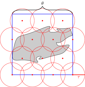

It is important to note that most of the parameters in Theorem 9 do not require a difficult analysis such that the bound (10) can be directly evaluated. While the computation of the exact covering number is a difficult problem for general sets , it can be easily upper bounded as illustrated in Fig. 1. For this reason, we overapproximate the set through a hypercube with edge length . Then, the covering number of is bounded by (Shalev-Shwartz and Ben-David, 2013)
which is by construction also a bound for the covering number of , i.e.,
Since a probabilistic Lipschitz constant of the unknown function is a preliminary requirement for suitable hyperparameters as explained in Section 4.2, the uniform error bound mainly depends on training data , the considered set , the probability and the virtual grid constant allowing the direct computation of the bound (10). Hence, it is trivially evaluated with very little computational complexity emphasizing its high applicability, especially in safe control of unknown systems which can require fast computation of bounds.
Furthermore, it is important to observe that the virtual grid constant balances the effect of the state space discretization and the inherent uncertainty measured by the posterior standard deviation . Therefore, can be made arbitrarily small by choosing s sufficiently fine virtual grid. This in turn increases and thus the effect of the posterior standard deviation on the bound. However, depends merely logarithmically on such that even poor Lipschitz constants , and can be easily compensated by small virtual grid constants . In the following subsection we exploit this trade-off to analyze the asymptotic behavior of our uniform error bound and show that convergence to zero can be achieved with suitable training data.
Remark 10
Since the standard deviation varies within the state space , an optimal virtual grid constant , which minimizes the expression for all , does not exist in general. While simple approaches such as choosing such that is negligible for all provide satisfying results in our simulations, more complex approaches remain open research questions.
4.4 Analysis of Asymptotic Behavior
A crucial question in safe reinforcement learning and control of unknown systems is the existence of lower bounds for the learning error since they determine the achievable control performance. It can be directly observed from Theorem 9 that the training data plays the critical role in this question since it affects the posterior standard deviation . By analyzing the asymptotic behavior of (10), i.e., considering the limit , we can derive conditions for the posterior variance which ensure that an arbitrarily small error can be achieved with suitable training data. This is shown in the following theorem.
Theorem 11
Consider a zero mean Gaussian process defined through the covariance kernel with continuous partial derivatives up to the fourth order on the set . Furthermore, consider an infinite data stream of observations of an unknown, Lipschitz continuous function which satisfies Assumptions 4.2 and 4.3. Let and denote the mean and standard deviation of the Gaussian process conditioned on the first observations. If there exists a class function and a constant such that
then the learning error uniformly converges to zero almost surely with rate
Compared to Theorem 9 this theorem does not require knowledge of the Lipschitz constant of the unknown function . However, it instead requires increased smoothness of the covariance kernel. This smoothness guarantees the existence of probabilistic maximum absolute values and Lipschitz constants due to Theorem 7 and Corollary 8, respectively, which is exploited together with Theorem 9 in the proof. Moreover, note that this theorem guarantees almost sure convergence, while previous versions in (Lederer et al., 2019) merely guaranteed convergence with arbitrary probability.
Although the asymptotic analysis is typically not performed for the related approaches in (Srinivas et al., 2012; Chowdhury and Gopalan, 2017), similar conditions for the posterior variance can be straightforwardly derived. Due to the dependence on the information gain of these approaches, the necessary decrease rate depends strongly on the covariance kernel . For example, the information gain behaves as for the squared exponential kernel which leads to the conditions for (Srinivas et al., 2012) and for (Chowdhury and Gopalan, 2017). For the Matérn kernel with smoothness parameter the information gain exhibits the asymptotic behavior such that for (Srinivas et al., 2012) and for (Chowdhury and Gopalan, 2017) are required. It can be clearly observed that in both cases the conditions on the posterior variance are far more restrictive than required by Theorem 11.
In addition to the weaker conditions of Theorem 11, it allows to directly pose a condition on the infinite training data sequence to ensure a vanishing uniform error bound by exploiting Theorem 3. This is shown in the following corollary.
Corollary 12
Consider a zero mean Gaussian process defined through the covariance kernel with continuous partial derivatives up to the fourth order on the set . Furthermore, consider an infinite sequence of observations of an unknown, Lipschitz continuous function which satisfies Assumptions 4.2 and 4.3. If there exists a function and a constant such that the assumptions of Theorem 3 are satisfied with for all , then the learning error uniformly converges to zero almost surely with rate
5 Safety Guarantees for Control of Unknown Dynamical Systems
When applying learning controllers in safety-critical applications like autonomous driving or robots working in close proximity to humans, upper bounds for the tracking error are crucial to provide formal safety guarantees for the dynamical systems. Therefore, we demonstrate how the results in the previous sections can be applied to design regulators for the safe control of unknown dynamical systems. A feedback linearization controller for robust tracking is presented in Section 5.1. In section 5.2 the stability of this controller is analyzed and the asymptotic behavior for infinite training data is investigated.
5.1 Tracking Control Design
We consider a nonlinear control affine dynamical system
| (11) |
with state and control input . Although we assume that the function is unknown, the structure of the dynamics is not. However, this is not a severe restriction since nonlinear control affine systems of the form (11) can be applied in a wide variety of applications such as Lagrangian dynamics and many physical systems.
Our goal is to determine a policy such that the output tracks the desired trajectory with vanishing tracking error where , i.e., . We assume that training data of the real system is available in the form of noisy observations , , such that we can train a Gaussian process and use its posterior mean function as a model estimate of the unknown function . Based on this model estimate we compensate the unknown non-linearity which is commonly referred to as feedback linearization for control affine systems (Khalil, 2002). After compensation of the non-linearity we apply linear regulators for the tracking such that we obtain the policy
| (12) |
with the linear controller for tracking
with control gain and filter coefficients , such that the polynomial with is Hurwitz (Hurwitz, 1895). The application of this policy leads to the error dynamics (Chowdhary et al., 2015)
| (13) |
The first addend corresponds to the nominal error dynamics, which are described by a linear system with dynamics matrix , while the second addend represents the effect of the learning error on the tracking error dynamics.
Remark 13
Our assumption on the available training data allows noisy observations of the derived state while the states themselves must be measured noise free. Although this assumption is debatable, it reflects practical implementation well due to the fact that the time derivative is typically realized with finite difference approximations. These approximations inject considerably more noise than direct measurements of the state .
5.2 Probabilistic Stability Analysis
For safety critical applications, e.g., when robots and human work in close proximity, it is crucial to formally verify that the controlled system satisfies safety constraints. This requires a sufficiently precise model and a properly chosen control gain as well as filter coefficients such that an upper bound on the tracking error can be determined as defined in the following.
Definition 14 (Ultimate Boundedness)
The tracking error between a dynamical system and a reference trajectory is ultimately bounded, if there exists a positive constant such that for every , there is a such that
As an analytical computation of the trajectories is generally impossible, we conduct a stability analysis based on Lyapunov theory. This analysis exhibits the advantage that conclusions about the closed-loop system behavior can be drawn without the necessity of simulating the controlled system or even executing the policy on the real system (Khalil, 2002). In the following, we consider a bounded reference trajectory in order to comply with the requirement of a compact state space for the uniform error bound of Gaussian process regression.
Lemma 15 ((Khalil, 2002))
Consider a dynamical system and a bounded reference trajectory . If there exists a positive definite (so called Lyapunov) function, , and a set for , such that
then the tracking error is ultimately bounded to the set for all .
Based on this lemma we can check the satisfaction of safety constraints by explicitly determining the set as shown in the following.
Theorem 16
Consider a control affine system (11), where admits a Lipschitz constant on , with feedback linearizing controller (12). Let the unique, positive definite solution to the algebraic Riccati equation
with defined in (13). Assume that satisfies 4.2 and the observations , , satisfy the conditions of 4.3. Consider the set of initial states and the Lyapunov decrease region defined as
with and from Theorem 9. If , then the tracking error converges with probability of at least for all to the ultimately bounded set
with ultimate bound
It is trivial to see that the ultimate bound and consequently the extension of the ultimately bounded set can be made arbitrarily small by reducing the posterior variance , which can be achieved by adding more training data. Therefore, it is straight forward to prove a vanishing control error in the limit of infinite training data, which is defined as asymptotic stability in control literature (Khalil, 2002). This is shown in the following corollary.
Corollary 17
Consider a control affine system (11), where satisfies 4.2 for a Gaussian process defined through the covariance kernel with continuous partial derivatives up to the fourth order on the set and the infinite observation sequence , , satisfies the conditions of 4.3. If the assumptions of Theorem 3 are satisfied with for all , then the tracking error satisfies the ultimate bound ultimate bound with probability of at least . Moreover, the feedback linearizing controller almost surely asymptotically stabilizes the system for all initial states in the limit of infinitely many training samples.
6 Numerical Evaluation
In this section we illustrate the behavior of the proposed bounds for the posterior variance, the learning error and the control error. Section 6.1 compares our variance bounds to the exact posterior variance and bounds from literature for different sampling distributions. In Section 6.2 we illustrate the importance of suitable prior distributions for meaningful uniform error bounds and evaluate the proposed constrained hyperparameter optimization. Finally, the data-dependency of the feedback linearizing controller is analyzed in Section 6.3 before it is applied to reference tracking with a real-world robotic manipulator in Section 6.4.
6.1 Decrease Rate of Posterior Variance Bounds
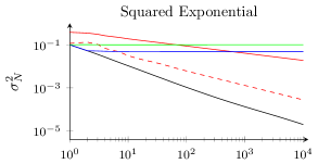
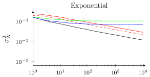
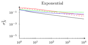
We compare the bounds in Theorem 1 and Corollary 2 to the exact posterior variance for GPs with a squared exponential, a Matérn kernel with , a polynomial kernel with and a neural network kernel. Furthermore, we evaluate the bound proposed in (Williams and Vivarelli, 2000), which considers the two closest points in the data set to the test point resulting in
where and are the distances to the two closest training samples and is the distance between the two closest training samples. Additionally, we consider the bound for the mean square prediction error proposed in (Wang and Haaland, 2018) which corresponds to a bound on the posterior variance. This bound is given by
where denotes the closest point in the training data set to the test point . The posterior variance is evaluated at the point for a uniform training data distribution . Furthermore, the length scale of the kernels is set to where applicable and the noise variance is set to . In order to obtain a good value for the information radius , consider the following approximation of (4) for isotropic kernels
where we use the expectation of instead of the random variable . For the squared exponential kernel the Taylor expansion around yields
Therefore, for large the best asymptotic behavior of (4) is achieved with for the squared exponential kernel under uniform sampling and leads to . The same approach can be used to calculate the information radius with the best asymptotic behavior of the bound in Corollary 2 for the Matérn kernel with . This leads to and an asymptotic behavior of . For the non-isotropic kernels, we pursue a similar approach and substitute the expected number of samples in (3), which results in the asymptotically optimal and . For the general bound in Theorem 1 we consider as reference point for the isotropic kernels, whereas we choose as reference point for the non-isotropic kernels because it exhibits higher variance and lies not on the boundary of the considered interval . The posterior variance bounds and the exact posterior variance averaged over training data sets are illustrated in Fig. 2.


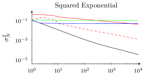
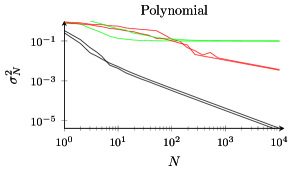
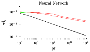
We also compare the bounds in Theorem 1 and Corollary 2 to the exact posterior variance for training data sampled from the distribution with density function
This probability density vanishes at the test point and it leads to for . By employing a Taylor expansion of the kernel around the test point, we can derive the optimal asymptotic decay rates for as in the previous section. For the Matérn kernel, this leads to and an asymptotic behavior of the posterior variance . For the squared exponential kernel, a slightly faster decreasing can be chosen, which results in . For the non-isotropic kernels we choose the reference point at such that it does not suffer from the vanishing distribution. Hence, we choose as for the uniform distributed training data. The resulting posterior variance bounds and the exact posterior variance are illustrated in Fig. 3.
The posterior variance bounds for the isotropic squared exponential and Matérn kernel exhibit a similar decrease rate as the actually observed one in Fig. 2 and Fig. 3. Indeed, the bound for the Matérn kernel shows the exact same behavior and only differs by a constant factor for large . However, for non-isotropic kernels, our bound in Theorem 1 is rather loose as it converges with while the true posterior variance exhibits a decay rate of approximately for the uniform distribution in Fig. 2. Furthermore, merely a small difference of the decrease rate of the numerically estimated posterior variance and our proposed bound can be observed between both figures. This is caused by the non-isotropy of the kernel and the bound: the kernel considers data globally, while our bound considers data locally around a non-local reference point . Finally, both of our proposed bounds are advantageous compared to existing approaches in the fact that they converge to a constant decrease rate, whereas the existing bounds converge to a constant value. Therefore, our bounds can be applied to for small as well as large numbers of training samples, while existing approaches work well only for small numbers of training samples.
6.2 Importance of Priors for Uniform Error Bounds
It is always possible to find a probability such that the uniform error bound (36) holds on the whole considered set . However, this value can be very small. Therefore, suitable hyperparameters are crucial to shape the prior distribution such that it assigns proper probability to the functions that coincide with the prior information and consequently, the uniform error bound holds with reasonably small values of . In order to demonstrate the effectiveness of incorporating prior information about maximum values and maximum derivative values through constraints on the hyperparameters, we compare the satisfaction of the uniform error bound (10) for constrained and unconstrained hyperparameters on two practically relevant scenarios.
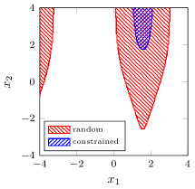
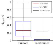
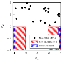
The first scenario considers the problem of choosing hyperparameters without any data, which is an issue that is typically avoided in applications such as sequential decision making by assuming randomly distributed measurements. In physical applications, however, there is typically no principled way for obtaining such initial data. Therefore, we assume random hyperparameters instead and enforce the constraints (9b) and (9c) by redrawing samples. We evaluate the performance on the function and consider the prior information , , , , and with probability . We investigate the uniform error bound with and on the region for a Gaussian process with isotropic squared exponential kernel. The signal standard deviation and the inverse length scale are drawn from the exponential distribution with mean and we perform simulation iterations. The violation of the uniform error bound for a constrained and unconstrained hyperparameter random sample is depicted on the left side of Fig. 4, while the right side illustrates the quotient of the violation surface and the total surface . Since the assumed bounds and are smaller than the actual function properties and the constraints (9b) and (9c) are merely necessary conditions, the satisfaction of the uniform error bound cannot be guaranteed in general for the chosen value of . However, the simulations clearly indicate that the constraints significantly reduce the constraint violation compared to purely random hyperparameters.
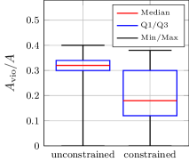
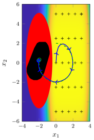
In the second scenario, we address the problem of training data which lies only on a small subset of the input domain such that the data only captures limited information of the true system. We consider the function and prior bounds , , , , and with probability . The error bound is investigated on with , and a probabilistic Lipschitz constant based on Corollary 8 with for a Matérn kernel with which is trained using training samples uniformly distributed on the set . The result of single simulation and the violation percentage over iterations of constrained and unconstrained hyperparameter optimization are depicted in Fig. 5. It can be clearly seen that the constraints (9b) and (9c) significantly contribute to the interpretability and reliability of the uniform error bound (10).
6.3 Data-dependency of Safety Regions for Learning-based Control
Due to the standard deviation dependence of the tracking error bound in Theorem 16, the guaranteed tracking performance is strongly influenced by the training data distribution and density. We investigate these relationships on a two-dimensional system of the form (11) with . In order to demonstrate the effect of the distribution, we use a uniform grid over with points and as training data set, such that half of the considered state space is not covered by training data. The impact of the training data density is showed by determining the tracking error for data sets with , , samples on a uniform grid over . We consider a circular reference trajectory and choose small gain controller gains and . A Gaussian process with automatic relevance determination is employed for regression and the hyperparameters are constrained with , and with probability according to (7) and (8). The Lipschitz constant is determined probabilistically using Corollary 8 with leading to a conservative value which is compensated by in Theorem 9. We combine Corollary 8 and Theorem 9 with using a union bound approximation.
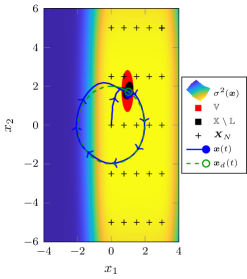
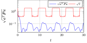

Figs. 6 and 7 depict the simulation results. It is clearly illustrated that training data has a crucial impact on the posterior variance and thus, a lack of samples causes a large ultimately bounded set . It can be observed that the ultimate bound strongly correlates with the size of the tracking error observed in simulation as shown on the left side of Fig. 7. However, the derived ultimate bound is rather conservative which is a consequence of the small violation probability of . Moreover, the tracking error and the ultimate bound decrease with a growing number of training samples, as illustrated on the right side of Fig. 7. In fact, it follows from Corollary 17 that with , as it is straightforward to derive that the uniform grid admits and . Since the asymptotic posterior variance bound for the squared exponential kernel is rather loose as outlined in Section 6.1, is also conservative and we can observe a faster decay rate of the ultimate bound in the simulations. Nevertheless, Corollary 17 is an important result since it guarantees a vanishing tracking error in the limit of infinite training data.
6.4 Safety Region Evaluation in Robotic Manipulator Simulations
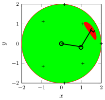
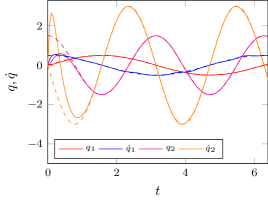
We investigate the tracking error bound in the real-world application of controlling a robotic manipulator with 2 degrees of freedom (DoFs) in simulation. The considered robotic manipulator, whose dynamics are derived according to (Murray et al., 1994, Chapter 4), has links with unit length and unit masses/ inertia. We assume that the Lipschitz constant is known and straightforwardly extend Theorem 9 to the multidimensional case based on the union bound. Since the considered robot has 2 DoFs, its state space is four dimensional and we evaluate the uniform error bound on . The GP is trained using samples, which are equally spaced in the region . For both DoFs, we use control gains and . The reference trajectories for tracking are sinusoidal as shown in Fig. 8 on the right side.
In order to visualize the tracking error bound in Theorem 16 in an illustrative way, we transform it from the state space into the task space as shown in Fig. 8 on the left. Exploiting only the learned dynamics, it can be guaranteed that the robot manipulator will not leave the depicted area, which thereby can be considered as safe. While similar theoretical results can be derived using previous error bounds for GPs, there applicability to these practical settings is severely limited due to
-
1.
they do not allow Gaussian observation noise on the training data (Srinivas et al., 2012), which is commonly assumed in control,
-
2.
they require constants, such as the maximal information gain in (Srinivas et al., 2010), which cannot be computed efficiently in practice,
-
3.
they base on assumptions, which are unintuitive and difficult to verify in practice (e.g., the RKHS norm of the unknown dynamical system (Berkenkamp et al., 2016b)).
7 Conclusion
This paper presents a novel uniform error bound for Gaussian process regression. By exploiting the inherent probability distribution of Gaussian processes instead of the RKHS attached to the covariance function, a wider class of functions can be considered. A novel method to compute interpretable hyperparameters based on prior knowledge is presented and the importance of suitably chosen hyperparameters is demonstrated for uniform error bounds. By deriving an analytical bound for the posterior variance of Gaussian processes and analyzing the asymptotic behavior of the bound it is shown that the derived uniform error bound converges to zero under weak assumptions on the training data distribution. The derived results are employed to develop a provably safe tracking control algorithm for which asymptotic stability in the limit of infinite training data is shown. The theoretical results are validated in simulations illustrating the behavior of the derived posterior variance bound, investigating the effect of badly chosen hyperparameters on uniform error bounds and demonstrating the safe tracking control of a robotic manipulator.
A Proofs for Posterior Variance Bounds
A.1 Variance Bounds
Proof [Proof of Theorem 1] Since is a positive definite, quadratic matrix, it follows that
Applying the Gershgorin theorem (Gershgorin, 1931) the maximal eigenvalue is bounded by
Furthermore, due to the definition of we have
Therefore, can be bounded by
| (14) |
This bound can be further simplified exploiting the fact that (Vivarelli, 1998) and considering only samples inside the ball with radius . Using this reduced data set instead of and writing the right side of (14) as a single fraction results in
| (15) |
where
Under the assumption that it follows from the Lipschitz continuity of that
Furthermore, it holds that
Therefore, can be bounded by
since .
Hence, the result is proven.
A.2 Asymptotic Behavior of Variance Bounds
Proof [Proof of Theorem 3] By setting in Theorem 1 and simplifying we obtain
Considering only the asymptotic behavior described by the -notation we therefore have
which proofs the theorem.
In order to prove Lemma 5 , some auxiliary results for binomial distributions are necessary. These are provided in the following Lemmas.
Lemma 18
The -th central moment of a Bernoulli distributed random variable is given by
| (16) |
Proof The polynom can be expanded as
The -th moment about the origin of the Bernoulli distribution is given by for (Forbes et al., 2011). Therefore, the expectation of this polynomial is given by
which directly yields the result.
Lemma 19
The -th central moment of a binomial distributed random variable with samples is bounded by
| (17) |
where are finite coefficients.
Proof A binomial random variable is defined as the sum of i.i.d. Bernoulli random variables . Therefore, the -th central moment of the binomial distribution is given by
Define the multinomial coefficient as
Then, the sum in the expectation can be expanded, which yields
| (18) |
This equation expresses the moments of the binomial distribution in terms of the moments of the Bernoulli distribution. Since the first central moment of every distribution equals , summands containing a equal . Therefore, we obtain the equality
| (21) |
Moreover, we have
with
due to Lemma 18. By substituting this into (21) we obtain
The product can have between and factors due to the structure of the problem. Therefore, it is not necessary for the sum to consider all coefficients , but rather consider only coefficients which are greater than . This leads to the following equality
| (24) |
Due to (Cormen et al., 2009) it holds that . Furthermore, the functions can be upper bounded by because . Therefore, we can upper bound the -th central moment of the binomial distribution by
with
| (27) |
and the result is proven.
The restriction to samples allows to derive a relatively simple expression for the expansion in (18). However, the bound (17) also holds without this condition, since it only guarantees that for , , and therefore, all possible combinations of can be estimated simpler in (24). Hence, the corresponding summands in (27) can be considered for and the upper bound (17) still holds for .
Based on these preliminary results we can state the proof of Lemma 5.
Proof [Proof of Lemma 5] We have to show that the number of samples from the probability distribution with density inside the balls with radius grows to infinity sufficiently fast. The number of samples follows a binomial distribution with mean
where
is the probability of a sample lying inside the ball around with radius for fixed . Since we have
by assumption, this mean exhibits a rate
Therefore, it is sufficient to show that converges to its expectation almost surely, which is identically to proving that
Due to the Borel-Cantelli lemma, this convergence is guaranteed if
| (28) |
holds for all . The probability for each can be bounded by
for each due to Chebyshev’s inequality, where the -th central moment of the binomial distribution can be bounded by
with some coefficients due to Lemma 19. Therefore, we can bound each probability in (28) by
Due to (6) this bound can be simplified to
where . Let . Then, each exponent is smaller than or equal to . Hence, the sum of probabilities can be bounded by
where is the Riemann zeta function, which has finite values. Therefore, we obtain
and consequently, the theorem is proven.
B Proofs for the Probabilistic Uniform Error Bound
B.1 Hyperparameter Bounds
In order to make the proof of Theorem 7 easier accessible, we split it up into the following auxiliary lemma and the main proof. The auxiliary lemma derives a bound for the expected supremum of a Gaussian process.
Lemma 20
Consider a Gaussian process with a continuously differentiable covariance function and let denote its Lipschitz constant on the set with maximum extension . Then, the expected supremum of a sample function of this Gaussian process satisfies
Proof We prove this lemma by making use of the metric entropy criterion for the sample continuity of some version of a Gaussian process (Dudley, 1967). This criterion allows to bound the expected supremum of a sample function by
| (29) |
where is the -packing number of with respect to the covariance pseudo-metric
Instead of bounding the -packing number, we bound the -covering number, which is known to be an upper bound. The covering number can be easily bounded by transforming the problem of covering with respect to the pseudo-metric into a coverage problem in the original metric of . For this reason, define
which is continuous due to the continuity of the covariance kernel . Consider the inverse function
Continuity of implies . In particular, this means that we can guarantee if . Due to this relationship it is sufficient to construct an uniform grid with grid constant in order to obtain a -covering net of . Furthermore, the cardinality of this grid is an upper bound for the -covering number, i.e.
Therefore, it follows that
Due to the Lipschitz continuity of the covariance function, we can bound by
Hence, the inverse function satisfies
and consequently
holds, where the ceil operator is resolved through the addition of . Substituting this expression in the metric entropy bound (29) yields
This integral can be solved similarly as shown in (Grünewälder et al., 2010) using the inequality
Through a change of variables we obtain
This integral can be bounded
which concludes the proof.
Based on the expected supremum of Gaussian process it is possible to
derive a high probability bound for the supremum of a sample function
which we exploit to proof Theorem 7 in the following.
Proof [Proof of Theorem 7] We prove this lemma by exploiting the wide theory of concentration inequalities to derive a bound for the supremum of the sample function . We apply the Borell-TIS inequality (Talagrand, 1994)
| (30) |
Due to Lemma 20 we have
| (31) |
We conclude the proof of this lemma by
substituting (31) in (30) and choosing
.
For the proof of Corollary 8 we make use of the fact that the derivative
of a sample function can be considered as a sample function from another Gaussian process.
Thus, we merely have to apply Theorem 7 to this new Gaussian process as
shown in the following.
B.2 Error Bound
Proof [Proof of Theorem 9] We first prove the Lipschitz constant bounds of the posterior mean and the posterior variance , before we derive the bound of the regression error. The norm of the difference between the posterior mean evaluated at two different points is given by
with
Due to the Cauchy-Schwarz inequality and the Lipschitz continuity of the kernel we obtain
which proves Lipschitz continuity of the mean . In order to bound the Lipschitz constant of the posterior variance we employ the Cauchy-Schwarz inequality to the absolute value of the difference of variances such that
| (32) |
On the one hand, we have
| (33) |
due to Lipschitz continuity of . On the other hand we have
| (34) |
The bound for the Lipschitz constant follows from substituting (33) and (34) in (32). The Lipschitz continuity of the posterior variance can be transferred to the posterior standard deviation. In order to see this more clearly observe that the difference of the variance at two points can be expressed as
Since the standard deviation is positive semidefinite we have
and hence, we obtain
Therefore, the difference of the posterior standard deviation at two points can be bounded by taking the square root of the Lipschitz constant multiplied with the distance between both points. Finally, we use these properties to prove the probabilistic uniform error bound by exploiting the fact that for every grid with grid points and
| (35) |
it holds with probability of at least that (Srinivas et al., 2012)
Choose , then
holds with probability of at least . Due to continuity of , and we obtain
Moreover, the minimum number of grid points satisfying (35) is given by the covering number . Hence, we obtain
where
B.3 Asymptotic Convergence
Proof [Proof of Theorem 11] Due to Theorem 9 with and the union bound over all it follows that
| (36) |
with probability of at least for . A trivial bound for the covering number can be obtained by considering a uniform grid over the cube containing . This approach leads to
where . Therefore, we have
| (37) |
Furthermore, the Lipschitz constant is bounded by
due to Theorem 9. Since the Gram matrix is positive semidefinite and is bounded by some with probability of at least for due to Theorem 7, we can bound by
where is a vector of i.i.d. zero mean Gaussian random variables with variance . Therefore, it follows that . Due to (Laurent and Massart, 2000), with probability of at least we have
Setting and applying the union bound over all yields
with probability of at least . Hence, the Lipschitz constant of the posterior mean function satisfies with probability of at least
Since grows logarithmically with the number of training samples , it holds that with probability of at least . The Lipschitz constant of the posterior variance can be bounded by
because . Moreover, the unknown function admits a Lipschitz constant with probability of at least with due to Corollary 8. Therefore, application of the union bound to (36) yields
with probability of at least . This function must converge to for in order to guarantee a vanishing regression error which is only ensured if decreases faster than . Therefore, set in order to guarantee
However, this choice of implies that due to (37). Since there exists an such that , by assumption, we have
| (38) |
with probability of at least for all
, and . It remains to show
that this holds with probability . We prove this by contradiction and consider
for notational simplicity in the following. Assume that
(38) holds not with probability . Then, there exists a
such that (38) holds with probability no more than
. However, we can set such that
(38) holds with probability of at least
which contradicts the assumption. Hence, (38) holds almost
surely and the proof is concluded.
C Stability Proofs for Robust Tracking Control
Proof [Proof of Theorem 16] Since is Hurwitz, there exists a unique, positive definite matrix such that (Khalil, 2002)
Based on this matrix , we define a quadratic Lyapunov function . The time derivative of this Lyapunov function is given by
where denotes the last column of the matrix . Using the uniform error bound from Theorem 9 and the definition of , we can bound this derivative by
Therefore, we obtain
If , we can apply Lemma 15 to characterize the ultimate bound by
References
- Beatson et al. (2010) Rick Beatson, Oleg Davydov, and Jeremy Levesley. Error Bounds for Anisotropic RBF Interpolation. Journal of Approximation Theory, 162(3):512–527, 2010.
- Beckers and Hirche (2018) Thomas Beckers and Sandra Hirche. Gaussian Process based Passivation of a Class of Nonlinear Systems with Unknown Dynamics. In Proceedings of the European Control Conference, pages 1257–1262, 2018.
- Berkenkamp and Schoellig (2015) Felix Berkenkamp and Angela P. Schoellig. Safe and Robust Learning Control with Gaussian Processes. In Proceedings of the European Control Conference, pages 2496–2501, 2015.
- Berkenkamp et al. (2016a) Felix Berkenkamp, Andreas Krause, and Angela P. Schoellig. Bayesian Optimization with Safety Constraints: Safe Automatic Parameter Tuning in Robotics. Technical report, ETH Zürich, Zürich, 2016a.
- Berkenkamp et al. (2016b) Felix Berkenkamp, Riccardo Moriconi, Angela P. Schoellig, and Andreas Krause. Safe Learning of Regions of Attraction for Uncertain, Nonlinear Systems with Gaussian Processes. In Proceedings of the IEEE Conference on Decision and Control, pages 4661–4666, 2016b.
- Berkenkamp et al. (2016c) Felix Berkenkamp, Angela P. Schoellig, and Andreas Krause. Safe Controller Optimization for Quadrotors with Gaussian Processes. In Proceedings of the IEEE International Conference on Robotics and Automation, pages 491–496, 2016c.
- Berkenkamp et al. (2017) Felix Berkenkamp, Matteo Turchetta, Angela P. Schoellig, and Andreas Krause. Safe Model-based Reinforcement Learning with Stability Guarantees. In Advances in Neural Information Processing Systems, pages 908–918, 2017.
- Chowdhary et al. (2015) Girish Chowdhary, Hassan A. Kingravi, Jonathan P. How, and Patricio A. Vela. Bayesian Nonparametric Adaptive Control using Gaussian Processes. IEEE Transactions on Neural Networks and Learning Systems, 26(3):537–550, 2015.
- Chowdhury and Gopalan (2017) Sayak Ray Chowdhury and Aditya Gopalan. On Kernelized Multi-armed Bandits. In Proceedings of the International Conference on Machine Learning, pages 844–853, 2017.
- Cormen et al. (2009) Thomas H. Cormen, Charles E. Leiserson, Ronald L. Rivest, and Clifford Stein. Introduction to Algorithms. The MIT Press, Cambridge, Massachusetts, third edition, 2009.
- Deisenroth et al. (2013) Marc P. Deisenroth, Gerhard Neumann, and Jan Peters. A Survey on Policy Search for Robotics. Foundations and Trends in Robotics, 2(1-2):1–142, 2013.
- Dicker et al. (2017) Lee H. Dicker, Dean P. Foster, and Daniel Hsu. Kernel Ridge vs. Principal Component Regression: Minimax Bounds and the Qualification of Regularization Operators. Electronic Journal of Statistics, 11(1):1022–1047, 2017.
- Ding et al. (2010) Li Ding, Hou Neng Wang, Zhi Hong Guan, and Jie Chen. Tracking under Additive White Gaussian Noise Effect. IET Control Theory and Applications, 4(11):2471–2478, 2010.
- Dudley (1967) Richard M. Dudley. The Sizes of Compact Subsets of Hilbert Space and Continuity of Gaussian Processes. Journal of Functional Analysis, 1(3):290–330, 1967.
- Forbes et al. (2011) Catherine Forbes, Merran Evans, Nicholas Hastings, and Brian Peacock. Statistical Distributions. Wiley, Hoboken, New Jersey, fourth edition, 2011.
- Gershgorin (1931) Semyon A. Gershgorin. Ueber die Abgrenzung der Eigenwerte einer Matrix. Bulletin de l’Academie des Sciences de l’URSS. Classe des sciences mathematiques et na, (6):749–754, 1931.
- Ghosal and Roy (2006) Subhashis Ghosal and Anindya Roy. Posterior Consistency of Gaussian Process Prior for Nonparametric Binary Regression. The Annals of Statistics, 34(5):2413–2429, 2006.
- Grünewälder et al. (2010) Steffen Grünewälder, Jean-Yves Audibert, Manfred Opper, and John Shawe-Taylor. Regret Bounds for Gaussian Process Bandit Problems. Journal of Machine Learning Research, 9:273–280, 2010.
- Hadidi and Schwartz (1979) Mohamed T. Hadidi and Stuart Schwartz. Linear Recursive State Estimators Under Uncertain Observations. IEEE Transactions on Automatic Control, 24(6):944–948, 1979.
- Helwa et al. (2019) Mohamed K. Helwa, Adam Heins, and Angela P. Schoellig. Provably Robust Learning-Based Approach for High-Accuracy Tracking Control of Lagrangian Systems. IEEE Robotics and Automation Letters, 4(2):1587–1594, 2019.
- Hurwitz (1895) A. Hurwitz. Ueber die Bedingungen, unter welchen eine Gleichung nur Wurzeln mit negativen reellen Theilen besitzt. Mathematische Annalen, 46(2):273–284, 1895.
- Huval et al. (2015) Brody Huval, Tao Wang, Sameep Tandon, Jeff Kiske, Will Song, Joel Pazhayampallil, Mykhaylo Andriluka, Pranav Rajpurkar, Toki Migimatsu, Royce Cheng-Yue, Fernando Mujica, Adam Coates, and Andrew Y. Ng. An Empirical Evaluation of Deep Learning on Highway Driving. pages 1–7, 2015. URL http://arxiv.org/abs/1504.01716.
- Kailath (1968) T Kailath. An Innovations Approach to Least-Squares Estimation. IEEE Transactions on Automatic Control, 13(6):646–655, 1968.
- Kanagawa et al. (2018) Motonobu Kanagawa, Philipp Hennig, Dino Sejdinovic, and Bharath K. Sriperumbudur. Gaussian Processes and Kernel Methods: A Review on Connections and Equivalences. pages 1–64, 2018. URL http://arxiv.org/abs/1807.02582.
- Khalil (2002) Hassan K. Khalil. Nonlinear Systems. Prentice-Hall, Upper Saddle River, NJ, third edition, 2002.
- Koller et al. (2018) Torsten Koller, Felix Berkenkamp, Matteo Turchetta, and Andreas Krause. Learning-based Model Predictive Control for Safe Exploration. In Proceedings of the IEEE Conference on Decision and Control, pages 6059–6066, 2018.
- Komaee (2012) Arash Komaee. Estimation of a Low-intensity Filtered Poisson Process in Additive White Gaussian Noise. IEEE Transactions on Automatic Control, 57(10):2518–2531, 2012.
- Laurent and Massart (2000) Beatrice Laurent and Pascal Massart. Adaptive Estimation of a Quadratic Functional by Model Selection. The Annals of Statistics, 28(5):1302–1338, 2000.
- Lederer et al. (2019) Armin Lederer, Jonas Umlauft, and Sandra Hirche. Uniform Error Bounds for Gaussian Process Regression with Application to Safe Control. In Advances in Neural Information Processing Systems, 2019.
- Lederer et al. (2020) Armin Lederer, Alexandre Capone, and Sandra Hirche. Parameter Optimization for Learning-based Control of Control-Affine Systems. In Learning for Dynamics and Control, volume 120, pages 1–11, 2020.
- Mendelson (2002) Shahar Mendelson. Improving the Sample Complexity using Global Data. IEEE Transactions on Information Theory, 48(7):1977–1991, 2002.
- Mercer (1909) James Mercer. Functions of Positive and Negative Type, and their Connection with the Theory of Integral Equations. Philosophical Transactions of the Royal Society A: Mathematical, Physical and Engineering Sciences, 209(441-458):415–446, 1909.
- Murray et al. (1994) Richard M. Murray, Zexiang Li, and S. Shankar Sastry. A Mathematical Introduction to Robotic Manipulation. CRC Press, 1994.
- Narcowich et al. (2006) Francis Narcowich, Joseph D. Ward, and Holger Wendland. Sobolev Error Estimates and a Bernstein Inequality for Scattered Data Interpolation via Radial Basis Functions. Constructive Approximation, 24(2):175–186, 2006.
- Neal (1996) Radford M Neal. Lecture Notes in Statistics: Bayesian Learning for Neural Networks. 1996.
- Nørgård et al. (2000) P. M. Nørgård, O. Ravn, N. K. Poulsen, and L. K. Hansen. Neural Networks for Modelling and Control of Dynamical Systems - A Practicioner’s Handbook. Springer, London, 2000.
- Opper and Vivarelli (1999) Manfred Opper and Francesco Vivarelli. General Bounds on Bayes Errors for Regression with Gaussian Processes. Advances in Neural Information Processing Systems, pages 302–308, 1999.
- Rasmussen and Williams (2006) Carl E. Rasmussen and Christopher K. I. Williams. Gaussian Processes for Machine Learning. The MIT Press, Cambridge, MA, 2006.
- Schaback (2002) Robert Schaback. Improved Error Bounds for Scattered Data Interpolation by Radial Basis Functions. Mathematics of Computation, 68(225):201–217, 2002.
- Schaback and Wendland (2006) Robert Schaback and Holger Wendland. Kernel Techniques: From Machine Learning to Meshless Methods. Acta Numerica, 15:543–639, 2006.
- Scheuerer et al. (2013) Michael Scheuerer, Robert Schaback, and Martin Schlather. Interpolation of Spatial Data - A Stochastic or a Deterministic Problem? European Journal of Applied Mathematics, 24(4):601–629, 2013.
- Shalev-Shwartz and Ben-David (2013) Shai Shalev-Shwartz and Shai Ben-David. Understanding Machine Learning: From Theory to Algorithms. Cambridge University Press, New York, NY, 2013.
- Shekhar and Javidi (2018) Shubhanshu Shekhar and Tara Javidi. Gaussian Process Bandits with Adaptive Discretization. Electronic Journal of Statistics, 12:3829–3874, 2018.
- Shi (2013) Lei Shi. Learning Theory Estimates for Coefficient-based Regularized Regression. Applied and Computational Harmonic Analysis, 34(2):252–265, 2013.
- Srinivas et al. (2010) Niranjan Srinivas, Andreas Krause, Sham Kakade, and Matthias Seeger. Gaussian Process Optimization in the Bandit Setting: No Regret and Experimental Design. In Proceedings of the International Conference on Machine Learning, pages 1015–1022, 2010.
- Srinivas et al. (2012) Niranjan Srinivas, Andreas Krause, Sham M. Kakade, and Matthias W. Seeger. Information-Theoretic Regret Bounds for Gaussian Process Optimization in the Bandit Setting. IEEE Transactions on Information Theory, 58(5):3250–3265, 2012.
- Stein (1999) Michael L. Stein. Interpolation of Spatial Data: Some Theory for Kriging. Springer Science & Business Media, 1999.
- Talagrand (1994) Michael Talagrand. Sharper Bounds for Gaussian and Empirical Processes. The Annals of Probability, 22(1):28–76, 1994.
- Umlauft and Hirche (2020) Jonas Umlauft and Sandra Hirche. Feedback Linearization Based on Gaussian Processes with Event-triggered Online Learning. IEEE Transactions on Automatic Control, 2020.
- Umlauft et al. (2017) Jonas Umlauft, Thomas Beckers, Melanie Kimmel, and Sandra Hirche. Feedback Linearization using Gaussian Processes. In Proceedings of the IEEE Conference on Decision and Control, pages 5249–5255, 2017.
- Umlauft et al. (2018) Jonas Umlauft, Lukas Pöhler, and Sandra Hirche. An Uncertainty-Based Control Lyapunov Approach for Control-Affine Systems Modeled by Gaussian Process. IEEE Control Systems Letters, 2(3):483–488, 2018.
- van der Vaart and van Zanten (2011) Aad van der Vaart and Harry van Zanten. Information Rates of Nonparametric Gaussian Process Methods. Journal of Machine Learning Research, 12:2095–2119, 2011.
- Vivarelli (1998) Francesco Vivarelli. Studies on the Generalisation of Gaussian Processes and Bayesian Neural Networks. PhD thesis, Aston University, 1998.
- Wang and Haaland (2018) Wenjia Wang and Benjamin Haaland. Controlling Sources of Inaccuracy in Stochastic Kriging. Technometrics, pages 1–13, 2018.
- Wendland (2004) Holger Wendland. Scattered Data Approximation. Cambridge University Press, 2004.
- Williams and Vivarelli (2000) Christopher K. I. Williams and Francesco Vivarelli. Upper and Lower Bounds on the Learning Curve for Gaussian Processes. Machine Learning, 40:77–102, 2000.
- Wu and Schaback (1993) Zong Min Wu and Robert Schaback. Local Error Estimates for Radial Basis Function Interpolation of Scattered Data. IMA Journal of Numerical Analysis, 13(1):13–27, 1993.