Learning and Fast Adaptation for Grid Emergency Control via Deep Meta Reinforcement Learning

Abstract

As power systems are undergoing a significant transformation with more uncertainties, less inertia and closer to operation limits, there is increasing risk of large outages. Thus, there is an imperative need to enhance grid emergency control to maintain system reliability and security. Towards this end, great progress has been made in developing deep reinforcement learning (DRL) based grid control solutions in recent years. However, existing DRL-based solutions have two main limitations: 1) they cannot handle well with a wide range of grid operation conditions, system parameters, and contingencies; 2) they generally lack the ability to fast adapt to new grid operation conditions, system parameters, and contingencies, limiting their applicability for real-world applications. In this paper, we mitigate these limitations by developing a novel deep meta-reinforcement learning (DMRL) algorithm. The DMRL combines the meta strategy optimization together with DRL, and trains policies modulated by a latent space that can quickly adapt to new scenarios. We test the developed DMRL algorithm on the IEEE 300-bus system. We demonstrate fast adaptation of the meta-trained DRL polices with latent variables to new operating conditions and scenarios using the proposed method, which achieves superior performance compared to the state-of-the-art DRL and model predictive control (MPC) methods.

I Introduction

POWER systems are facing increased risks of large outages due to main factors including aging infrastructure, significant change of generation/load mix [1], extreme weather[2], threats from physical and cyber attacks. This is evident by increasing occurrence of large outages [2, 3]. In this context, corrective and emergency control is imperative in real-time operation to minimize the occurrence and impact of power outages and blackouts [4, 5]. Furthermore, improved emergency control capabilities help the industry reduce overly relying on, thus the cost of, preventive security measures, thereby achieving overall better efficiency and asset utilization [6].

Recently, deep reinforcement learning (DRL) made outstanding progress [7, 8] and showed promising results for providing fast and effective power system stability and emergency control solutions [9, 5, 10]. The standard formulation of reinforcement learning (RL) is to maximize the average (or expected) accumulative rewards over the considered scenarios of the environments [11]. However, for power systems with many significantly different operation conditions and increased uncertainties, the policy learned by DRL may not work well when the grid operation condition changes notably at the testing or deployment stage, leading to unsatisfactory or even unacceptable system performance and outcomes.

One approach to partially addressing the issue is moving the RL training as close as possible to the real operation time to reduce the uncertainties (thus the variance of operation conditions has to be considered) by shortening the required training time. We developed the parallel augmented random search (PARS) algorithm that is highly scalable to accelerate the training in our previous work[12]. However, a fundamental yet generally missing capability for RL agents (controllers) is to quickly adapt to new grid operation conditions. Indeed, researchers in [13] pointed out ensuring the adapability of machine learning models is a requirement for practical acceptance of machine learning applications. The adaptability problem in the power system emergency control area has not been addressed yet. In this paper, we tackle this problem by developing a novel deep meta-reinforcement learning (DMRL) algorithm and applying it to learn and adapt power system emergency control policies against voltage stability issues. The proposed DMRL algorithm can quickly adapt the behavior of the trained policies to unseen scenarios in a new target environment. It combines the meta strategy optimization together with DRL, and trains a policy modulated by a latent space that can quickly adapt to new and much different grid operation conditions, and system parameters. Given fast-changing operation conditions and increased uncertainties in power systems, we believe this work is a major advancement for DRL application for grid control.

I-A Literature review

There are a number of recent efforts in applying RL (particularly DRL) for power system stability and emergency control [14, 15, 16, 17, 9, 18, 5]. However, there are some notable limitations among them: (1) they trained a single policy to handle many different power grid environments with the so-called domain randomization technique [19] and simply relied on the unwarranted generalization capability of deep neural networks to generalize to unseen grid environments, thus the trained polices may not work well if the grid environment changes drastically; (2) they lacked the capability of fast adaptation to new grid environments by leveraging prior learning experience.

In machine learning literature, existing works in adapting control policies to new environments are mainly in the following two categories: 1) model-based adaption methods; 2) model-free adaptation methods. In model-based adaptation methods[20, 21], a dynamic model is first learnt using some data-driven techniques to capture or represent the system dynamics in the training environment, and then the learnt dynamic model is adapted with some recent observations from the target environment, and finally the control policy is determined using methods such as model predictive control (MPC)[21]. These methods can adapt to changes in the environment on-line. However, there are two main shortcomings in terms of application for large-scale power system emergency control: 1) learning good dynamic models of large-scale, highly non-linear power systems is highly challenging, and has yet proven practically feasible; 2) solving large-scale MPC to obtain optimal control policy is computationally expensive[12], and thus almost impossible to meet the real-time requirement of power grid emergency control.

In model-free adaption methods, the control policy (modeled as a neural network) is directly adjusted according to the observed dynamics from the targeted environment. One popular class of such methods is the gradient-based meta learning approach [22, 23]. However, gradient-based approaches usually require small incremental parameter adjustment to stabilize the learning process or ensure numerical stability [24]. Thus, without a large amount of experience (adaption steps) to update the control policy parameters, the meta-learnt control policy could not be significantly adjusted to adapt to a quite different environment.

Another class of the model-free methods is latent space-based adaptation method [25, 26]. It encodes the training experience into a latent context (space), and the control policy is conditioned on the latent context. The latent context is then fine-tuned for new environments. Most efforts in this line of research are to first train an inference model in conjunction with the RL training process during the training stage, and during adaption, leverage the inference model to infer the latent context through the observation input from the target environment. However, when the target or actual environment differs notably from those considered in the training, the inference model may produce non-optimal results, leading to poor adaptation performance. As pointed out in [26], this is mainly due to the fact that the process of learning latent context in training and inferring the suitable latent context in adaptation are not consistent. By extending the same latent space optimization process from the meta-learning stage to both meta-learning and adaptation stages to overcome such discrepancy, Yu et al. [26] developed the so-called meta strategy optimization (MSO) method and showed that it allows the agents to learn better latent space that is suitable for fast adaptation to new environments. In our work, we adapted this technique for power system emergency control problems.

I-B Contributions

Our contributions in this paper include the following:

1. We develop a novel DMRL algorithm that combines the PARS [12] and MSO [26] algorithms, which could train an agent that can quickly and effectively adapt to a new environment.

2. The developed DMRL algorithm consists of a meta-learning stage and an adaptation stage (see Fig. 4), which naturally fits into the execution time frame of existing power system operation procedures.

3. We apply the developed DMRL algorithm for training power system emergency control policies against voltage stability problems and more importantly fast adapting them to unseen operation conditions and/or contingency scenarios.

4. We demonstrate fast and effective adaptation of the meta-trained DRL polices to new operation scenarios including unseen power flow cases, new system dynamic parameters and new contingencies using the proposed method and the testing results show superior performance compared to other baseline methods.

While we focus on grid emergency control applications in our test cases in this paper, the proposed method is generic and could be extended to other control and decision-making problems in power systems without much difficulty.

I-C Organization of the paper

The rest of the paper is organized as follows: Section II introduces the problem formulation and our proposed method at a high level. Section III presents the details of our proposed DMRL algorithm. Test cases and results are shown in Section IV. Conclusions and future work are provided in Section V.

II Problem Statement and Proposed Method

We first discuss the challenges in applying DRL for grid control under fast-changing power grid operation scenarios with increased uncertainties, which necessitates and highlights the need of fast adaptation capability for DRL-based agents or controllers. Then, we introduce meta-reinforcement learning techniques for achieving the fast adaptation. Lastly, we present the key procedures of our proposed DMRL approach and how they fit into existing power grid operation procedures.

II-A Challenges in Applying RL for Grid Control under Fast-Changing Operation Scenarios with Increased Uncertainties

RL problems can be defined as policy search in a (partially observable) Markov Decision Process (MDP) defined by a tuple ($\mathcal{S,A}$,$p$,$r$,$\gamma$) [11], where $\mathcal{S}$ is the state space, $\mathcal{A}$ is the action space, $p:\mathcal{S}\times\mathcal{A}\rightarrow\mathcal{S}$ is the transition function, and $r$: $\mathcal{S}\times\mathcal{A}\rightarrow\mathbb{R}$ is the reward function. The goal of RL is to learn a policy $\pi(s_{t}):\mathcal{S}\rightarrow\mathcal{A}$, such that it maximizes the expected accumulative reward $J(\pi)$ over time under $p$:

$$J(\pi)=\mathbb{E}_{s_{0},a_{0},s_{1},a_{1},...s_{\mathcal{T}},a_{\mathcal{T}}}\Sigma_{t=0}^{\mathcal{T}}\gamma^{t}r\left(s_{t},a_{t}\right)$$ (1)

where $a_{t}\sim\pi(s_{t})$ and $s_{t+1}\sim p(s_{t},a_{t})$, and $\mathcal{T}$ is the maximum end time. Note that the accumulated reward maximization in RL is opposite to minimizing the cost objective that are usually considered in power system optimizations. A standard setup of RL problems for power grid control is shown in Fig. 1. In DRL, the policy is usually parameterized by a neural network with weights $\theta$ and the policy is denote as $\pi_{\theta}$.

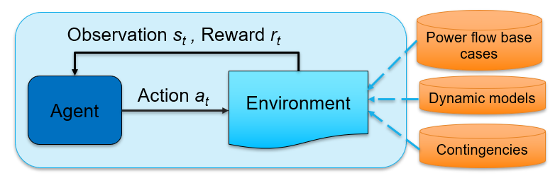
Figure 1: The agent-environment interaction in a Markov decision process

There are increased uncertainties in power systems due to large integration of intermittent generation resources, as illustrated in Fig. 2. The system operation conditions could change tremendously even within a few hours (for example, the so-called duck curve [27]). Since RL training (usually ranging from hours to days) is slow compared to the required real-time emergency control time interval (i.e., within seconds), RL training has to be performed off-line, from hours to days ahead of real-time operation (denoted by time $T$ in Fig. 2). Since the actual operation conditions and contingency scenarios cannot be pre-determined accurately prior to their occurrence, a number of operation conditions (different power flows and system dynamic parameters) have to be considered as a distribution of different environments $\bm{P}(E_{i})$ while the potential contingencies have to be considered as a distribution of different contingencies $\bm{P}(\mathcal{C}_{j})$ when training the RL agent (or policy). The DRL algorithms typically perform well on the set of training environments $\{\bm{\mathcal{E}}_{trn}\}$ and they purely leverage the trained neural networks $\pi_{\theta}$ to learn representations that support generalization to a new target environment $\mathcal{E}_{tar}$. As a result, the success or effectiveness of generalization to a new environment $\mathcal{E}_{tar}$ dependent on the similarity between new target environment $\mathcal{E}_{tar}$ and the training environment set $\{\bm{\mathcal{E}}_{trn}\}$. In other words, the generalization may not be effective if the power grid operation conditions become quite different from those considered at the training stage.

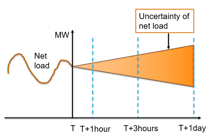
Figure 2: Uncertainties in power systems

II-B Meta-reinforcement Learning

Meta-reinforcement learning (Meta-RL) integrates the idea of meta-learning (learning to learn) into RL. The goal of Meta-RL is to train an agent that can quickly adapt to a new task using only a few data points and training iterations. To accomplish this, the model or learner is trained at a meta-learning stage on a set of tasks, such that the trained model can quickly adapt to new tasks using only a small number of examples or trials. Formally, given a distribution of tasks $\bm{P}(T_{k})$ that we are interesting in and an adaptation process $U:\Theta\times\bm{P}(T_{k})\mapsto\Theta$, Meta-RL finds a policy that maximizes the rewards after adaptation:

$$\theta^{*}=\arg\max_{\theta}\mathbb{E}_{\bm{P}(T_{k})}[J(U(\theta,T_{k}))]$$ (2)

Note that for the power grid emergency control problem we investigated in this paper, the distribution of tasks is defined by a distribution of environments presenting different system conditions and dynamic parameters, that is $\bm{P}(T_{k})=\bm{P}(E_{i})$.

An ideal Meta-RL algorithm should: 1) be data efficient during adaptation to new tasks; 2) flexibly modulate the behavior of the trained policy to achieve optimal performance for new tasks.

II-C Our Proposed Method

We propose a latent-space-based MSO algorithm to address the Meta-RL problem defined in (2) by extracting the training experience on the distribution of tasks $\bm{P}(T_{k}))$ into a latent space representation [26], as illustrated in Fig. 3.

A key idea behind MSO is that we want to obtain a universal policy that performs optimally for every training task in $\bm{P}(T_{k})$. More importantly, this universal policy needs to be able to quickly adapt to novel tasks, which are not seen in $\bm{P}(T_{k})$. We first make the universal policy conditioned on the training tasks $\bm{P}(T_{k})$ so that the policy can learn a specialized strategy for each training task. However, training such a policy is a challenging problem because $\bm{P}(T_{k})$ is high-dimensional, which can significantly increase the input size and the complexity of the neural networks of the policy. Since this high-dimensional task space is often redundant, our method finds a lower-dimensional representation (latent space) of the training tasks $\bm{P}(T_{k})$. This learned low-dimensional representation is then used to encode the task and augment the original input of the control policy. More concretely, the proposed method defines the universal policy to be $\pi_{\theta}(s_{t},c):\mathcal{S}\times\mu\mapsto\mathcal{A}$, where $c$ is a latent vector in the low-dimensional latent space $\mu$. During training time, MSO jointly optimizes the latent space $\mu$ and the policy parameters $\theta$ such that the learned controller can effectively handle novel tasks with a small amount of fine-tuning data. In other words, MSO finds a non-linear dimension reduction of the training tasks $\bm{P}(T_{k})$, guided by the reward of the control policy after adaptation. Given a novel task during the testing stage, our algorithm performs adaptation by identifying the task in the latent space, through finding an optimal latent vector $c$, which combines with the universal policy $\pi_{\theta}(s_{t},c)$, can perform best in the test task. Since the latent space is low dimensional, the adaptation is data efficient. Furthermore, our learning algorithm trains the meta-learning model based on a set of representative forecasted system environments $\{\bm{\mathcal{E}}_{trn}\}$ with uncertainties being taken into account, therefore the latent representation $\mu$ can be learnt efficiently with good physical information and prior knowledge about the distributions of the system environments.

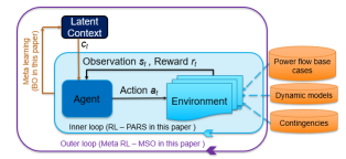
Figure 3: Latent-space based meta-reinforcement learning

We integrate the MSO idea with the highly-scalable PARS algorithm to develop a novel DMRL algorithm that can quickly adapt to the new target power grid environment $\mathcal{E}_{tar}$ (herein a new power grid environment can be either a new power flow condition, or new set of system dynamic parameters or a combination of both). The key idea is illustrated in Fig. 4. The DMRL algorithm includes three stages:

1. meta-training;

2. adaptation;

3. real-time deployment.

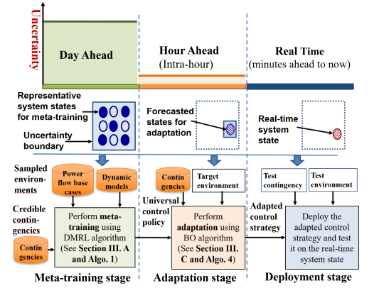
Figure 4: An illustration of application of the proposed method for grid control and its fitting into existing grid operation stages (or time frames). (Note: While all the states are shown within the forecasted operation boundary here, which is valid most of the time, we acknowledge that there are some rare situations where the system operation state at the adaptation stage or deployment stage might be out of the boundary considered during the meta-training stage. We have tested such rare conditions in Section IV.)

At the day-ahead meta-training stage, our work is based on the fact that grid operators do not have the exact information of load and generation patterns, load dynamics, and the exact fault locations and durations, and that they usually have some prior knowledge about system uncertainties based on historical operation data in the day-ahead operation as illustrated in Fig. 2. Therefore, we propose to train a meta-learning model based on a set of representative forecasted system environments $\{\bm{\mathcal{E}}_{trn}\}$. The meta-learning stage produces a well-trained universal policy $\pi_{\theta}(s,c)$ that is conditioned on and can work for a distribution of different environments $\bm{P}(\{\bm{\mathcal{E}}_{trn}\})$. Note that if the system operation conditions do not change notably from day to day, this meta-training stage is not required to perform every day, because the universal policy model can be reused.

At the hour-ahead (or intra-hour) adaptation stage, within a short period of time (from 5 minutes to 1 hour) before actual real-time operation, improved forecast of the power grid states with much less uncertainty is obtained and thus the target environment $\mathcal{E}_{tar}$ can be constructed. For fast adaptation, we directly use the well-trained universal policy $\pi_{\theta}(s,c)$ from the meta-learning stage, and optimize the latent vector $c(\mathcal{E}_{tar})$ to adapt it to the target environment $\mathcal{E}_{tar}$. Consequently, an adapted control strategy $\pi_{\theta}(s,c(\mathcal{E}_{tar}))$ (i.e, an optimized universal policy combined with the optimized latent vector) for the target grid environment is created. With this proposed procedure of meta-learning and adaptation, much less time will be required during the adaptation stage for a target or new environment. Thus, it can meet the real-time operation requirements.

At the deployment stage, the adapted DMRL-based control strategy will be tested for the real-time emergency control. The testing environment could still have a small (i.e., 1% to 2% short-term forecasting errors [28]) difference from the specific target environment we consider at the adaptation stage. As we will shown in Section IV, the generalization capability of the DMRL model can accommodate and handle such small difference well.

In terms of fitting into real-world power grid operation procedures, the three stages discussed above directly correspond to day-ahead, hour-ahead, and real-time operation time frames, and improve forecasting over time.

III Deep meta reinforcement learning

In this section, we present the key algorithms and implementation details of our proposed DMRL method. Fig. 5 shows the flowchart and connections of the meta-learning, adaptation, and testing stages of the proposed DMRL method.

Figure 5: Flow Chart of the three stages of the proposed DMRL Method

III-A Deep Meta-Reinforcement Learning through Meta-Strategy Optimization

We propose a novel DMRL algorithm that combines the MSO and PARS algorithms to solve the meta-learning problem defined in (2). Our proposed method learns a latent-vector-conditioned policy on a distribution of Environments $\bm{P}(E_{i})$ representing forecasted grid operation conditions (different power flows and system dynamic parameters), and can quickly adapt the trained policy to a new target environment. Assuming that the distribution of Environments $\bm{P}(E_{i})$ defined in Section II could be represented by a latent space $\mu$, as explained in Section II.C, MSO extends the standard RL policy learning by training a universal policy $\pi_{\theta}(s,c)$ that is conditioned on the latent vector $c$ in the latent space $\mu$, $c\in\mu$. We can train such a universal policy with any standard RL algorithm by treating the latent vector $c$ as part of the observations [29]. The trained universal policy will change its behaviors with respect to different latent vectors in the latent space, thus a policy with a particular latent vector input $c\in\mu$ can be treated as one control strategy, which is trained to be optimal for one task in $\bm{P}(E_{i})$ as defined in Section II.

At the meta-training stage, we target at learning a universal policy $\pi_{\theta}(s,c)$ conditioned on a distribution of environments $\bm{P}(E_{i})$. We need to determine the corresponding latent vectors in the latent space, ${\bm{c}\in\mu}$, for a set of training environments $\bm{\mathcal{E}}\in\bm{P}(E_{i})$. Given that our goal is to find a set of strategies that work well for the set of training environments $\bm{\mathcal{E}}\in\bm{P}(E_{i})$, a direct approach is to use the performance of the training environments, i.e., the accumulated reward of the training environment as the metric to search the optimal strategies. Mathematically, we reformulate (2) and solve the following optimization problem on a distribution of environments $\bm{P}(E_{i})$ at the meta-training stage:

$$\theta^{\ast}=\arg\max_{\theta}\mathbb{E}_{\bm{\mathcal{E}}\in\bm{P}(E_{i})}\left[\max_{c\in\mu}{J}\left(c,\theta\right)\right],$$ (3)

where $\theta$ is the weight of the policy network, $J\left(c,\theta\right)$ is the expected accumulative reward of the strategy $\pi_{\theta}(s,c)$ on the environment $\mathcal{E}\in\bm{P}(E_{i})$, and $c$ is the latent vector that encodes the power grid operation condition environment $\mathcal{E}$ in the low-dimensional latent space $\mu$, $c\in\mu$. It is rather challenging to directly solve (3) because the optimization of $J(c,\theta)$ is inside the expectation of the objective term, and every single evaluation of $\theta$ requires solving a optimization problem to find the optimized latent vector $c$ to maximize $J(c,\theta)$, which is computationally expensive. To overcome this, we revise (3) as:

$$\theta^{\ast},c\left(\mathcal{E}\right)^{\ast}=\arg\max_{\theta,c(\mathcal{E})}\mathbb{E}_{\bm{\mathcal{E}}\in\bm{P}(E_{i})}\left[{J}\left(c(\mathcal{E}),\theta\right)\right],$$ (4)

where $c(\mathcal{E})$ is the specific latent vector that encodes the specific training environment $\mathcal{E}$ in the low-dimensional latent space $\mu$, $\mathcal{E}\in\bm{P}(E_{i})$ and $c(\mathcal{E})\in\mu$. Then, we can solve the optimization problem in (4) by solving two related optimization problems defined in (5) and (6) in an alternative manner, where $k$ is the iteration number.

$$c(\mathcal{E})_{k+1}=\arg{\max_{c}{J}}\left(c,\theta_{k}\right),\forall\mathcal{E}\in\bm{P}(E_{i})$$ (5)

$$\theta_{k+1}=\arg\max_{\theta}\mathbb{E}_{\mathcal{E}\in\bm{P}(E_{i})}\left[J\left(c(\mathcal{E})_{k},\theta\right)\right]$$ (6)

Note that (5) defines the strategy optimization (SO) problem to optimize the latent vector $c(\mathcal{E})$ for a strategy $\pi_{\theta}(s,c)$ and it will be solved by the Bayesian optimization (BO) described in Subsection III.C, and (6) defines a RL problem to determine the policy network parameters $\theta$ and could be solved by DRL algorithms. We solve (6) using PARS algorithm presented in the following subsection. Algorithm 1 gives the details of the proposed DMRL algorithm solving (5) and (6). As shown in Algorithm 1 and Fig. 5, the meta-learning algorithm includes two loops, the outer BO loop and the inner PARS loop. In the outer BO loop, for each iteration, we keep the weights $\theta$ of the universal policy $\pi_{\theta}(s,c)$ fixed and sample $K$ different environments $\mathcal{E}_{i}|i=1,2,..,K$. We use Bayesian optimization to update the optimal latent vector $c(\mathcal{E}_{i})$ for each corresponding sampled environment $\mathcal{E}_{i}$ by solving (5). Note that during the Bayesian optimization to update the optimal latent vector $c(\mathcal{E}_{i})$, for each different environments $\mathcal{E}_{i}$, we sample a total of $Q$ different contingencies. In the inner PARS loop, for each iteration, we sample $M$ different scenarios $\Gamma_{m\in M}=\{\mathcal{E}_{i\in K}\cup\mathcal{C}_{j\in Q}\}$, which is the combination of $K$ different environments $\mathcal{E}$ and $Q$ different contingencies $\mathcal{C}$. We keep the latent vector $c(\mathcal{E}_{i})$ for each sampled environment $\mathcal{E}_{i}$ fixed and use PARS to update the weights $\theta$ of the universal policy $\pi_{\theta}(s,c)$ by solving (6). At the end, this stage generates a well-trained universal policy $\pi_{\theta}(s,c)$ that is conditioned on the optimized latent vectors and works well for the sampled environments from the distribution of the environments $\bm{P}(E_{i})$.

At the adaptation stage, we target at transferring the universal policy $\pi_{\theta}(s,c)$ trained with DMRL in Algorithm 1 at the meta-learning stage to a target environment $\mathcal{E}_{tar}\in\bm{P}(E_{i})$. We need to determine the corresponding latent vector $c(\mathcal{E}_{tar})$ of the strategy $\pi_{\theta}(s,c)$ for the new specific target environment $\mathcal{E}_{tar}$. Mathematically, at the adaptation stage, we need to solve the strategy optimization (SO) problem defined in (5) for only a specific target environment $\mathcal{E}_{tar}$, which could achieve high computational efficiency. Algorithm 2 gives the details of the proposed adaptation algorithm to optimize the specific latent vector $c(\mathcal{E}_{tar})$ for the target environment $\mathcal{E}_{tar}$. As shown in Algorithm 2 and Fig. 5, we sample $P$ different contingencies $\mathcal{C}_{j}|j=1,2,..,P$ and optimize the latent vector $c(\mathcal{E}_{tar})$ against the $P$ different contingencies for this specific target environment $\mathcal{E}_{tar}$. Note also that in the proposed DMRL method, we adopt the same strategy optimization process to optimize the latent vector for the policy at both the meta-training and adaptation stages prior to testing/deployment. The outcome of the adaptation stage is a specific optimized strategy (an optimized universal policy $\pi_{\theta}(s,c)$ together with the optimized specific latent vector $c(\mathcal{E}_{tar})$) for the specific target environment $\mathcal{E}_{tar}$, and this optimized strategy is robust to a wide range of different contingencies.

Algorithm 1 Deep Meta-Reinforcement Learning (DMRL)

1:  initialize policy weights $\theta_{0}$ with random small numbers

2:  initialize latent vectors $\bm{c}(\mathcal{E})_{0}$ as $\bm{0}$

3:  for outer_iter $k$ = 0 to $N_{out}$ do

4:     sample $K$ Environments {$\mathcal{E}_{i}|i=1,2,..,K$}

5:     for each $\mathcal{E}_{i}$, sample $Q$ Contingencies $\mathcal{C}_{j}|j=1,2,..,Q$, solve (5) using Bayesian optimization with fixed $\theta_{k}$ and update corresponding latent vector $c(\mathcal{E}_{i})_{k}$

6:     for inner_iter $q$ = 0 to $N_{in}$ do

7:        sample $M$ Scenarios $\Gamma_{m\in M}=\{\mathcal{E}_{i\in K}\cup\mathcal{C}_{j\in Q}\}$

8:        update $\theta_{k}$ by solving (6) with the PARS algorithm with fixed $\bm{c}(\mathcal{E})_{k}$ as part of the observation

9:     end for

10:  end for

11:  return  $\theta_{k}$, $\bm{c}(\mathcal{E})_{k}$

Algorithm 2 Adaptation

1:  define the specific target environment $\mathcal{E}_{tar}$ for adaptation

2:  load policy weights $\theta_{train}$ from the outcome of Algorithm 1

3:  initialize the specific latent vector $c(\mathcal{E}_{tar})$ for the target environment $\mathcal{E}_{tar}$ as $\bm{0}$

4:  for adapt_iter $i$ = 0 to $N_{adapt}$ do

5:     sample $P$ Contingencies $\mathcal{C}_{j}|j=1,2,..,P$

6:     solve (5) using Bayesian optimization with fixed $\theta_{train}$ and update the specific latent vector $c(\mathcal{E}_{tar})$

7:  end for

8:  return  the optimized specific latent vector $c(\mathcal{E}_{tar})$

III-B Parallel Augmented Random Search

Augmented random search(ARS) is a derivative-free, efficient, easy-to-tune and robust-to-train RL algorithm[30]. In our previous work[12], we developed the PARS algorithm to scale up the ARS algorithm for large-scale grid control problems and reduce the training time. Specifically, we proposed and and implemented a novel nest parallelism scheme for ARS on a high-performance computing platform. The key steps of PARS algorithm are shown in Algorithm 3, with more details presented in [12]. We use it to solve the RL problem defined with (6) in the DMRL Algorithm 1.

Algorithm 3 Parallel Augmented Random Search (PARS)

1:  Initialize: Policy weights $\theta_{0}$, the running mean of observation states $\mu_{0}=\mathbf{0}\in\mathbb{R}^{n}$ and the running standard deviation of observation states $\Sigma_{0}=\mathbf{I}_{n}\in\mathbb{R}^{n}$, the total iteration number $H$.

2:  for iteration $t=1,...,H$ do

3:     sample $N$ random directions $\delta_{1},...,\delta_{N}$ with the same dimension as policy weights $\theta$

4:     for each $\delta_{i}(i\in[1,...,N])$ do

5:        add $\pm$ perturbations to policy weights: $\theta_{ti+}=\theta_{t-1}+\upsilon\delta_{i}$ and $\theta_{ti-}=\theta_{t-1}-\upsilon\delta_{i}$

6:        do total $2M$ Scenarios (episodes) denoted by $R_{\Gamma_{m\in M}}$, calculate the average rewards for $\pm$ perturbations

7:        During each episode, normalize states $s_{t,k}$ and obtain the action $a_{t,k}$, and new states $s_{t,k+1}$. Update $\mu_{t}$ and $\Sigma_{t}$ with $s_{t,k+1}$

8:     end for

9:     sort the directions based on $\max[r_{ti+},r_{ti-}]$ and select top $b$ directions, calculate their standard deviation $\sigma_{b}$

10:     update the policy weight:

$$\theta_{t+1}=\theta_{t}+\frac{\alpha}{b\sigma_{b}}\sum\limits_{i=1}^{b}(r_{ti+}-r_{ti-})\delta_{i}$$ (7)

11:     Step size $\alpha$ and standard deviation of the exploration noise $\upsilon$ decay with rate $\varepsilon$: $\alpha=\varepsilon\alpha$, $\upsilon=\varepsilon\upsilon$

12:  end for

13:  return  $\theta$

III-C Strategy Optimization through Bayesian Optimization

We propose to use Bayesian optimization (BO)[31] to solve the SO problem defined with (5) in the DMRL Algorithm 1, which can handle noisy and often non-convex objectives. BO is a parameter optimization method for any black-box objective function f(x). The core idea of BO is to conduct sequential sampling to construct the target function. BO consists of two key elements, a probabilistic surrogate model, which is a distribution over the target function, and an acquisition function, which is used to explore the parameter space based on the surrogate model. The surrogate model P(f) can be expressed as follows:

$$P(f|{x_{1:t}},{y_{1:t}})=\frac{{P({x_{t}},{y_{t}}|f)P(f|{x_{1:t-1}},{y_{1:t-1}})}}{{P({x_{t}},{y_{t}})}}$$ (8)

where $x_{1:t}$ is a matrix containing all the inputs from time step 1 to $t$, and $y_{1:t}$ is a vector containing the corresponding outputs, i.e., $y_{t}$ = $f(x_{t})$. The next input $x_{t+1}$ is selected by minimizing the following expected loss:

$${x_{t+1}}=\mathop{\arg\min}\limits_{{x_{t+1}}}\int{{\delta_{t}}(f,{x_{t+1}})dP(f|{x_{1:t}},{y_{1:t}})}$$ (9)

where $\delta_{t}(f,x_{t+1})$ is called the regret function, which measures the difference between the sampling point $x_{t+1}$ and the optimal point $x^{*}$.

However, in reality, since we do not have the knowledge of the optimum $x^{*}$, (9) cannot be applied directly. An acquisition function $\alpha_{t}(x)$ is designed instead as a proxy of the regret function. Namely, (9) becomes:

$${x_{t+1}}=\arg{\min_{x_{t+1}}}{\alpha_{t}}(x)$$ (10)

Some options for the acquisition function include probability of improvement (PI), expected improvement (EI), and upper confidence bound (UCB). In this work, we use UCB as the acquisition function, which has the following expression:

$${x_{t+1}}=\arg{\max_{x_{t+1}}}(\mu_{t}(x)+\kappa*\sigma_{t}(x))$$ (11)

In (11), $\mu_{t}(x)$ and $\sigma_{t}(x)$ are the mean and standard deviation of a Gaussian Process(GP), and $\kappa$ is the weight factor.

The overall process of applying BO to solve (5) is shown in Algorithm 4. Note that for (5), the BO objective function $f(x)$ is the expected accumulative reward $J(c,\theta)$ with only $c$ as the optimization variable $x$, since the $\theta$ is fixed for (5).

Algorithm 4 Bayesian Optimization

1:  initialize the sampling set $D$, probabilistic surrogate model $P(J(c,\theta_{fix}))$, solution $c$, and acquisition function $\alpha_{t}(c;D)$

2:  for $t=1,2,...,N_{BO}$ do

3:     select ${c_{t+1}}=\arg{\min_{c_{t+1}}}{\alpha_{t}}(c;D)$

4:     calculate $y_{t+1}=J(c_{t+1},\theta_{fix})$

5:     update the sampling set $D=D\cup(c_{t+1},y_{t+1})$

6:     update $P(J(c,\theta_{fix}))$ and $\alpha_{t}(c_{t+1};D)$

7:  end for

8:  return the solution $c$

IV Test cases and Results

IV-A The FIDVR problem and MDP formulation

Fault-induced delayed voltage recovery (FIDVR) is defined as the phenomenon whereby system voltage remains at significantly reduced levels for several seconds after a fault has been cleared [32]. The root cause is stalling of air-conditioner (A/C) motors and prolonged tripping. FIDVR events occurred in many utilities in the US. The industry have concerns over FIDVR issues since residential A/C penetration is at an all-time high and continues to grow. A transient voltage recovery criterion is defined to evaluate the system voltage recovery. Without loss of generality, we referred to the standard shown in Fig. 6 [33]. The objective of emergency control for FIDVR problem is to shed as little load as possible to recover voltages to meet the voltage recovery criterion.

Figure 6: Transient voltage recovery criterion for transmission system [33]

Key elements of the MDP formulation of this problem are:

1. Environment: The grid environment is simulated with RLGC [5, 34]. We considered a modified IEEE 300-bus system with loads larger than 50 MW within Zone 1 represented by WECC composite load model [35]. We prepared a wide range of power flow cases and considered different combinations of dynamic load parameters that are key for FIDVR problems for both training and testing.

2. Action: Load shedding control actions are considered for all buses with dynamic composite load model at Zone 1 (46 buses in total). The percentage of load shedding at each control step could be from 0 to 20%. The agent is designed to provide control decisions (including no action as an option) to the grid every 0.1 second.

3. Observation: The observations included voltage magnitudes at 154 buses within Zone 1, as well as the remaining fractions of 46 composite loads. Thus the dimension of the observation space is 200. The agent needs to obtain the observations from the grid environment every 0.1 second.

4. Reward: the reward $r_{t}$ at time $t$ is defined as follows:

   $$r_{t}=\begin{cases}-10000,\text{ if }V_{i}(t)<0.95,\quad t>T_{pf}+4\\ c_{1}\sum_{i}\Delta V_{i}(t)-c_{2}\sum_{j}\Delta P_{j}(t)-c_{3}u_{iv},\text{ otherwise}\end{cases}$$ (12)

   $$\Delta V_{i}(t)=\begin{cases}min\left\{V_{i}(t)-0.7,0\right\},\text{ if }{\scriptstyle T_{pf}<t<T_{pf}+0.33}\\ min\left\{V_{i}(t)-0.8,0\right\},\text{ if }{\scriptstyle T_{pf}+0.33<t<T_{pf}+0.5}\\ min\left\{V_{i}(t)-0.9,0\right\},\text{ if }{\scriptstyle T_{pf}+0.5<t<T_{pf}+1.5}\\ min\left\{V_{i}(t)-0.95,0\right\},\text{ if }{\scriptstyle T_{pf}+1.5<t}\end{cases}$$

   where $T_{pf}$ is the time instant of fault clearance, $V_{i}(t)$ is the bus voltage magnitude for bus $i$ in the power grid, $\Delta P_{j}(t)$ is the load shedding amount in p.u. at time step $t$ for load bus $j$, and $u_{iv}$ is the invalid action penalty. $c_{1},c_{2},$ and $c_{3}$ are weight factors.

5. Other details such as the state transition can be found in [5].

TABLE I: Power flow conditions for training

Training power flow case	Generation	Load
1	Total 22929.5 MW (100%)	Total 22570.2 MW (100%)
2	120% for all generators	120% for all loads
3	135% for all generators	135% for all loads
4	115% for all generators	150% for loads in Zone 1

TABLE II: Power flow conditions for adaptation and testing

	Adaptation		Testing
Adaptation/testing power flow case	Generation	Load	Generation	Load
1	90% for all generators	90% for all loads	92.4% for all generators	92.4% for all loads
2	110% for all generators	110% for all loads	107.7% for all generators	107.7% for all loads
3	115% for all generators	115% for all loads	117.2% for all generators	117.2% for all loads
4	125% for all generators	125% for all loads	122.5% for all generators	122.5% for all loads
5	140% for all generators	140% for all loads	142.1% for all generators	142.1% for all loads
6	95% for all generators	82.8% for loads in Zone 1	97.1% for all generators	85.32% for loads in Zone 1
7	107% for all generators	124.4% for loads in Zone 1	104.6% for all generators	121.5% for loads in Zone 1
8	110% for all generators	134.3% for loads in Zone 1	112.3% for all generators	137.2% for loads in Zone 1
9	119% for all generators	159.7% for loads in Zone 1	121.1% for all generators	162.6% for loads in Zone 1

TABLE III: Dynamic models for training and testing

	A/C Motor Percentage	$\bm{T_{stall}}(s)$	$\bm{V_{stall}}(p.u.)$
Training	44%	0.032	0.45
Testing	55%	0.075	0.495
	55%	0.1	0.53
	44%	0.1	0.53
	35%	0.05	0.45

IV-B Performance metrics and baselines

1. Metrics for training and adaptation: we target at day-ahead training (less than 24 hours) and hour-ahead policy adaptation (less than 60 minutes).

2. Metrics for testing: (a) the total solution time should be within 1 s for an event lasting 8 s to meet the real-time response requirement, or in other words, the average solution time should be within $0.0125$ s for each control step (80 steps in total); (b) the average reward on the testing scenarios set (the reward measures the optimality of the load shedding controls); (c) total load shedding amount.

We compared our method with PARS, one state-of-the-art DRL method, as well as the MPC method that provides (near) optimal solutions of the problem.

IV-C Training, adaptation and testing of control strategies

The meta-learning, adaptation and testing were performed on a local high-performance computing cluster using 1152 cores.

At the day-ahead meta-learning stage, since we do not know the exact load/generation pattern, as well as the load dynamics and the exact fault location and duration, we train a universal LSTM policy on 4 different environments and 18 different contingencies. Table I defines the power flow conditions for training. We consider 18 different contingencies, which are a combination of 2 fault durations (0.05 and 0.08 s) and 9 candidate fault buses (2, 3, 5, 8, 12, 15, 17, 23, 26) in the contingency set $\{C_{train}\}$ for training.

The hyperparameters of the DMRL algorithm for the training is shown in Table IV. Fig. 7 shows the average rewards with respect to training iterations for both the DMRL and PARS algorithms. DMRL and PARS has very similar convergence speed at the training stage. Table V shows the training time for both the DMRL and PARS methods. While the meta-training using BO method costs 2 more hours, the DMRL method can meet the day-ahead training requirement. The day-ahead meta-training produces one well-trained universal LSTM policy.

To comprehensively evaluate the proposed method, we perform adaptation and testing with 9 different power flow cases and 4 different set of dynamic models in this paper (a total of 36 different environments), as shown in Table II and Table III. Note that only one adaptation is usually needed for one system at one operation time instance in real-world application. We recognize that due to unpredicted and extreme situations, the load/generation pattern and the load dynamics of the specific target environments at the adaptation stage will not always be within the boundary considered in the training data set. Accordingly, we include some “outliers” in Table II and Table III. We believe such a testing setup can help to comprehensively test the adaptation and generalization capabilities of the proposed method.

At the intra-hour adaptation stage, we assume the grid operators have a much better estimation of the load/generation pattern and of the load dynamics, but cannot accurately forecast the fault location nor its duration. To validate that the proposed adaptation Algorithm 2 can work for a wide range of target environments that are different from the training environments, we defined a total of 36 different target environments for adaption $\{\mathcal{E}_{adapt}\}$, which are combinations of 9 different power flow conditions shown in Table II and 4 different sets of critical dynamic load parameters shown in Table III. Since we still cannot predict the fault location and duration accurately, for each target environment for adaptation $\mathcal{E}_{target,i}$, we sample the contingency set $\{C_{sample}\}$ and it has 102 different contingencies, which are combinations of 34 different fault buses and three different fault durations (0.06, 0.1 , and 0.18 second). Note that $\{C_{sample}\}$ is totally different from $\{C_{train}\}$. We generate different optimized latent vector for each different target environment in $\{\mathcal{E}_{adapt}\}$ separately. Table V shows that the adaptation for one environment takes 14.1 minutes, demonstrating that our method can meet the intra-hour adaptation time requirement.

At the testing stage, as shown in Table II, we assume the testing environment still has some small (e.g., 2.1% to 2.5% [28]) differences in terms of load, generation and net load when compared with the specific target environment we consider at the adaptation stage. Note that there is a one-to-one correspondence between adaptation and testing in terms of power flow condition, as shown in Table II. Therefore, we have a total of 36 specific target environments for testing and evaluation. For each target environment, we test the corresponding optimized control strategy on the contingency set $\{C_{test}\}$ that has 40 different contingencies with different fault buses and the fault duration being randomly sampled within the range between 0.05 second and 0.2 second. In summary, at the testing stage, we test the proposed DMRL method on a total of $36\times 40=1440$ different test scenarios.

TABLE IV: Hyperparameters for training 300-bus system

Parameters	300-Bus
Policy Model	LSTM
Policy Network Size (Hidden Layers)	[64,64]
Number of Directions ($N$)	128
Top Directions ($b$)	64
Step Size ($\alpha$)	1
Std. Dev. of Exploration Noise ($\upsilon$)	2
Decay Rate ($\varepsilon$)	0.996
BO iterations ($N_{BO}$)	32
Inner loop iteration ($N_{in}$)	20
Outer loop iteration ($N_{out}$)	25
Sampled environments ($K$)	3
Sampled contingencies ($Q$)	12
Sampled scenarios ($M$)	36

IV-D Performance evaluation

Table V shows the average computation time of the DMRL, PARS, and MPC methods for determining the control actions for each testing scenario. The event duration for each testing scenario is 8 s. As discussed in Section IV.A, all the three methods (DMRL, PARS, and MPC) obtain the observations from the grid simulation environment and provide control actions back to it every 0.1 s. Thus, there are a total of 80 control steps with 0.1 s time step. The “testing time” listed in the Table V is the average “total computation time” for the whole 80 control steps for each testing scenario. That is, both DMRL and PARS take 0.009 s on average to compute control actions within the 0.1 s control interval. Therefore, both methods meet the “real-time” requirements for the load shedding actions for the FIDVR problem in real system. In contrast, the MPC method takes 0.79 s computational time to determine the actions per control action step, which does not meet the “real-time” requirements for the load shedding actions. The reason is that performing neural network forward pass to infer actions in the DMRL and PARS approaches is much more efficient than solving a complex optimization problem with the MPC method.

Figure 7: Learning curves of DMRL and PARS.

TABLE V: Comparison of computation time for PARS, DRML, and MPC

	Required	DMRL	PARS	MPC
Training	$<$ 24 hours	11.6 hours	9.5 hours	–
Adaptation	$<$ 60 mins	14.1 mins	–	–
Testing	$<$ 1 s	0.72 s	0.72 s	63.31 s

To show the advantage of our DMRL method, we calculated the reward differences (i.e., the reward of DMRL subtracts that of PARS ) for all 1440 different test scenarios. A positive value means the proposed DMRL method performs better for the corresponding Fig. 8 shows the histogram of rewards differences for the 1440 different scenarios. Among 94.69% of those scenarios, DMRL outperforms PARS since most of the reward differences are positive when compared with PARS. This confirms that with a learnt latent vector for each target environment, DMRL-based agent can better distinguish each environment and tailor the control strategy accordingly, thereby achieving overall better control effectiveness and performance. Furthermore, there are 88 scenarios where DMRL successfully recovered the system voltage above the performance requirement shown in Fig. 6 while PARS failed to do so. These scenarios are corresponding to a cluster of scenarios with reward difference of about +20000 in Fig. 8. Indeed, this result demonstrates the unwarranted generalization capability of DRL algorithms for some new or unseen grid environments while our DMRL algorithm can successfully fast adapt to unseen (even very different from those in the training set) grid operation environments.

Figure 8: Histogram of the reward differences between DMRL and PARS.

Fig. 9 shows the comparison of DMRL, PARS and MPC performance for a test scenario with a three-phase fault at bus 26 lasting 0.15 second. The total rewards of PARS, DMRL and MPC methods are -25833, - 2715 and - 2742, respectively. Fig. 9(A) shows that the voltage with PARS (red curve) at bus 32 could not recover to meet the standard (dashed black curve), while with DMRL (blue curve) and MPC (green curve), voltages could be recovered to meet the performance standard. Further investigation indicated there were 11 buses that could not recover their voltage with the PARS method, while the DMRL and MPC methods successfully recovered all bus voltages above the required levels. Fig. 9(B) shows that the load shedding amount with the DMRL method is less than that of PARS, while being the same as the MPC method, suggesting that DMRL can achieve (near) optimal solutions with fast adaptation.

Figure 9: Test results for a FIDVR event triggered by a three-phase fault at bus 26 of the IEEE 300-bus system. (A) Voltage of bus 32. The dash line denotes the performance requirement for voltage recovery. (B) Total load shedding amount.

V Conclusions

In this paper, we developed a novel DMRL algorithm to enable DRL agents to learn a latent context from prior learning experience and leverage it to quickly adapt to new (i.e., unseen during training time) grid environments, which could be new power flow conditions, dynamic parameters or combinations of them. The key idea in our method is integrating meta strategy optimization (MSO), which is a latent-space based meta-learning algorithm, with one state-of-the-art parallel ARS (PARS) algorithm. In addition, the meta-training and adaption procedures fit well into the execution time frames of the existing grid operation practice. We demonstrate the performance of the DMRL algorithm on a variety of different scenarios with the IEEE 300-bus system and compare it with PARS and MPC methods. The DMRL algorithm can successfully adapt to new power flow conditions and system dynamic parameters in less than 15 minutes. The performance of the adapted DMRL-based control polices is notably better than that of the PARS algorithm, and comparable to that of the MPC solutions. Furthermore, our method can provide control decisions in real-time while MPC fails to do so.

Future research topics of interest include:

1. Application of the developed technique for other grid stability controls and in other areas such as distribution system control, microgrid and building management where adaptation of control strategies is also a key issue.

2. Transferring learnt control policies for one area to a different area of the power system or even a different power system.

References

- [1] Australian Energy Market Operator, “Black system South Australia 28 September 2016 - Final Report,” March 2017. [Online]. Available: https://www.aemo.com.au/-/media/Files/Electricity/NEM/Market_Notices_and_Events/Power_System_Incident_Reports/2017/Integrated-Final-Report-SA-Black-System-28-September-2016.pdf
- [2] A. Kenward and U. Raja, “Blackout: Extreme weather climate change and power outages,” Climate central, vol. 10, pp. 1–23, 2014.
- [3] Z. Bo, O. Shaojie, Z. Jianhua, and et al, “An analysis of previous blackouts in the world: Lessons for china’s power industry,” Renewable and Sustainable Energy Reviews, vol. 42, pp. 1151–1163, feb 2015.
- [4] L. Wehenkel and M. Pavella, “Preventive vs. emergency control of power systems,” in IEEE PES Power Systems Conference and Exposition, 2004., Oct 2004, pp. 1665–1670 vol.3.
- [5] Q. Huang, R. Huang, W. Hao, J. Tan, R. Fan, and Z. Huang, “Adaptive power system emergency control using deep reinforcement learning,” IEEE Transactions on Smart Grid, vol. 11, no. 2, pp. 1171–1182, 2020.
- [6] G. Strbac, I. Konstantelos, and R. Moreno Vieyra, “Emerging modelling capabilities for system operations,” http://hdl.handle.net/10044/1/28453, Tech. Rep., March 2015.
- [7] D. Silver, J. Schrittwieser, and et al, “Mastering the game of go without human knowledge,” Nature, vol. 550, no. 7676, p. 354, 2017.
- [8] Y. Li, “Deep reinforcement learning: An overview,” arXiv preprint arXiv:1701.07274, 2017.
- [9] M. Glavic, “(deep) reinforcement learning for electric power system control and related problems: A short review and perspectives,” Annual Reviews in Control, vol. 48, pp. 22–35, 2019.
- [10] D. Cao, W. Hu, J. Zhao, G. Zhang, B. Zhang, Z. Liu, Z. Chen, and F. Blaabjerg, “Reinforcement learning and its applications in modern power and energy systems: A review,” Journal of Modern Power Systems and Clean Energy, vol. 8, no. 6, pp. 1029–1042, 2020.
- [11] R. S. Sutton and A. G. Barto, Reinforcement learning: An introduction. MIT press, 2018.
- [12] R. Huang, Y. Chen, T. Yin, X. Li, A. Li, J. Tan, W. Yu, Y. Liu, and Q. Huang, “Accelerated derivative-free deep reinforcement learning for large-scale grid emergency voltage control,” IEEE Transactions on Power Systems, vol. 37, no. 1, pp. 14–25, 2021.
- [13] L. Duchesne, E. Karangelos, and L. Wehenkel, “Recent developments in machine learning for energy systems reliability management,” Proceedings of the IEEE, vol. 108, no. 9, pp. 1656–1676, 2020.
- [14] Z. Yan and Y. Xu, “Data-driven load frequency control for stochastic power systems: A deep reinforcement learning method with continuous action search,” IEEE Transactions on Power Systems, vol. 34, no. 2, pp. 1653–1656, 2018.
- [15] Y. Xu and Z. Yan, “A multi-agent deep reinforcement learning method for cooperative load frequency control of a multi-area power system,” IEEE Transactions on Power Systems, vol. 35, no. 6, pp. 4599–4608, 2020.
- [16] Q. Li, Y. Xu, and C. Ren, “A hierarchical data-driven method for event-based load shedding against fault-induced delayed voltage recovery in power systems,” IEEE Transactions on Industrial Informatics, 2020.
- [17] R. Diao, Z. Wang, D. Shi, Q. Chang, J. Duan, and X. Zhang, “Autonomous voltage control for grid operation using deep reinforcement learning,” in 2019 IEEE Power & Energy Society General Meeting (PESGM). IEEE, 2019, pp. 1–5.
- [18] C. Chen, M. Cui, F. F. Li, S. Yin, and X. Wang, “Model-free emergency frequency control based on reinforcement learning,” IEEE Transactions on Industrial Informatics, 2020.
- [19] J. Tobin, R. Fong, A. Ray, J. Schneider, W. Zaremba, and P. Abbeel, “Domain randomization for transferring deep neural networks from simulation to the real world,” in 2017 IEEE/RSJ International Conference on Intelligent Robots and Systems (IROS). IEEE, 2017, pp. 23–30.
- [20] A. Nagabandi, I. Clavera, S. Liu, R. S. Fearing, P. Abbeel, S. Levine, and C. Finn, “Learning to adapt in dynamic, real-world environments through meta-reinforcement learning,” arXiv preprint arXiv:1803.11347, 2018.
- [21] I. Lenz, R. A. Knepper, and A. Saxena, “DeepMPC: Learning deep latent features for model predictive control.” in Robotics: Science and System, 2015. [Online]. Available: http://www.roboticsproceedings.org/rss11/p12.pdf
- [22] C. Finn, P. Abbeel, and S. Levine, “Model-agnostic meta-learning for fast adaptation of deep networks,” arXiv preprint arXiv:1703.03400, 2017.
- [23] C. Finn and S. Levine, “Meta-learning and universality: Deep representations and gradient descent can approximate any learning algorithm,” arXiv preprint arXiv:1710.11622, 2017.
- [24] M. Botvinick, S. Ritter, J. X. Wang, Z. Kurth-Nelson, C. Blundell, and D. Hassabis, “Reinforcement learning, fast and slow,” Trends in cognitive sciences, vol. 23, no. 5, pp. 408–422, 2019.
- [25] K. Rakelly, A. Zhou, C. Finn, S. Levine, and D. Quillen, “Efficient off-policy meta-reinforcement learning via probabilistic context variables,” in International conference on machine learning. PMLR, 2019, pp. 5331–5340.
- [26] W. Yu, J. Tan, Y. Bai, E. Coumans, and S. Ha, “Learning fast adaptation with meta strategy optimization,” IEEE Robotics and Automation Letters, 2020.
- [27] Q. Hou, N. Zhang, E. Du, M. Miao, F. Peng, and C. Kang, “Probabilistic duck curve in high pv penetration power system: Concept, modeling, and empirical analysis in china,” Applied Energy, vol. 242, pp. 205–215, 2019.
- [28] J. Li, D. Deng, J. Zhao, D. Cai, W. Hu, M. Zhang, and Q. Huang, “A novel hybrid short-term load forecasting method of smart grid using mlr and lstm neural network,” IEEE Transactions on Industrial Informatics, 2020.
- [29] W. Yu, J. Tan, C. K. Liu, and G. Turk, “Preparing for the unknown: Learning a universal policy with online system identification,” arXiv preprint arXiv:1702.02453, 2017.
- [30] H. Mania, A. Guy, and B. Recht, “Simple random search of static linear policies is competitive for reinforcement learning,” in Advances in Neural Information Processing Systems, 2018, pp. 1800–1809.
- [31] J. Mockus, Bayesian approach to global optimization: theory and applications. Springer Science & Business Media, 2012, vol. 37.
- [32] NERC, “A technical reference paper fault-induced delayed voltage recovery,” 2009.
- [33] PJM Transmission Planning Department, “Exelon transmission planning criteria,” 2009.
- [34] Q. Huang, R. Huang, and W. Hao, “An open-source platform for applying reinforcement learning for grid control,” https://github.com/RLGC-Project/RLGC, accessed: 2020-12-10.
- [35] Q. Huang, R. Huang, B. J. Palmer, Y. Liu, S. Jin, R. Diao, Y. Chen, and Y. Zhang, “A generic modeling and development approach for WECC composite load model,” Electric Power Systems Research, vol. 172, pp. 1–10, 2019.