Toward Data Cleaning with a Target Accuracy:
A Case Study for Value Normalization

Abstract.

Many applications need to clean data with a target accuracy. As far as we know, this problem has not been studied in depth. In this paper we take the first step toward solving it. We focus on value normalization (VN), the problem of replacing all string that refer to the same entity with a unique string. VN is ubiquitous, and we often want to do VN with 100% accuracy. This is typically done today in industry by automatically clustering the strings then asking a user to verify and clean the clusters, until reaching 100% accuracy. This solution has significant limitations. It does not tell the users how to verify and clean the clusters. This part also often takes a lot of time, e.g., days. Further, there is no effective way for multiple users to collaboratively verify and clean. In this paper we address these challenges. Overall, our work advances the state of the art in data cleaning by introducing a novel cleaning problem and describing a promising solution template.

1. Introduction

Data cleaning (DC) has been a long-standing challenge in the database community. Many DC problems have been studied, such as cleaning with a budget, cleaning to satisfy constraints but minimize changes to the data, etc. Recently, however, we have seen another novel DC problem in industry: cleaning with a target accuracy, e.g., with at least 95% precision and 90% recall. While pervasive, this problem appears to have received little attention in the research community.

In this work, we take the first step toward solving this problem. We focus on value normalization (VN), the problem of replacing all strings (in a given set) that refer to the same real-world entity with a unique string. VN is ubiquitous, and industrial users often want to do VN with 100% accuracy.

Example 1.1.

To enable product browsing by brand on walmart.com, the business group at WalmartLabs asks the IT group to normalize the brands, e.g., converting those in Figure 1.a into those in Figure 1.b. If some brands are not normalized correctly, then customers may not find those products, resulting in revenue losses. So the business group asks the IT group to ensure that the brands are normalized with 100% accuracy.

Many enterprise customers of Informatica (which sells data integration software) also face this problem, in building business glossaries, master data management, and knowledge graph construction. In general, if even a small amount of inaccuracy in VN can cause significant problems for the target application, then the business group will typically ask the IT group to help perform VN with 100% accuracy.

Figure 1. An example of normalizing product brands

In response, the IT group typically employs an algorithm to cluster the strings, then asks a user to verify and clean the clusters. Consider the five brands in Figure 2.a. The IT group applies an algorithm to produce two clusters $c_{1}$ and $c_{2}$ (Figure 2.b). A user $U$ manually verifies and cleans the clusters, by moving “Vizio Corp” from cluster $c_{1}$ to $c_{2}$, producing the two clusters $c_{3}$ and $c_{4}$ in Figure 2.c. Finally, $U$ replaces each string in a cluster with a canonical string, producing the VN result in Figure 2.d.

Typically, a data scientist performs the “machine” part that clusters the strings, then a data analyst performs the “human” part that verifies and cleans the clusters. The IT group assures the business group that the resulting output is 100% accurate because a data analyst has examined it (assuming that he/she does not make mistakes).

While popular, the above solution has significant limitations. First, there is no precise procedure that a user can follow to execute the “human” part. So users often verify and clean in an ad-hoc, suboptimal, and often incorrect fashion. This also makes it impossible to understand the assumptions under which the solution reaches 100% accuracy and to formally prove it.

Second, the “human” part often incurs a huge amount of time, e.g., days. In contrast, the “machine” part often takes mere minutes. (In most cases that we have seen, users verified and cleaned using Excel, in a slow and tedious process.) So it is critical to develop a better solution and GUI tool to minimize the time of the “human” part.

Finally, it is difficult for multiple users to collaboratively verify and clean, even though this setting commonly occurs in practice.

Figure 2. A popular solution in industry to perform VN with 100% accuracy.

In this paper we develop Winston, a solution for the above challenges. (In the movie “Pulp Fiction”, Winston Wolfe is the fixer who cleans up messes made by other gangsters.) We first define a set of basic operations on a GUI for users, e.g., selecting a value, verifying if a cluster is clean, merging two clusters, etc. Then we provide precise procedures involving these actions that users can execute to verify/clean clusters. We prove that if users execute these actions correctly, then the output has 100% accuracy.

To minimize the time of the “human” part, we adopt an RDBMS-style solution. Specifically, we compose the GUI operations with clustering algorithms to form multiple “machine-human” plans, each executes the VN pipeline end-to-end. Next, we estimate the total time a user must spend per plan, select the plan with the least estimated time, execute its machine part, then show the output of that part to the user so that he/she can verify and clean it using a GUI (following the sequence of user operations that this plan specifies).

Finally, we show how to extend our solution to effectively divide the verification and cleaning work among multiple users.

Our solution appears highly effective. Section 8 shows that using the existing solution, a single user needs 29 days, 4.4 years, and 11.5 years to verify/clean 100K, 500K, and 1M strings, respectively. Winston drastically reduces these times to just 13 days, 9.6 months, and 1.3 years, using 1 user, and to 4.25 days, 2.2 months, and 3.5 months, using 3 users.

In summary, we make the following contributions:

• We formally define the novel data cleaning problem of VN with 100% accuracy. As far as we know, this paper is the first to study this problem in depth.

• We propose Winston, a novel RDBMS-style solution. Winston defines complex human operations and optimizes the human time of a plan. This is in contrast to traditional RDBMSs which define machine operations and optimize machine time.

• We describe extensive experiments (comparing Winston to a tool in a company, to the popular open-source tool OpenRefine, and to state-of-the-art string matching and entity matching solutions) that show the promise of our approach.

Overall, our work advances the state of the art in data cleaning by introducing a novel cleaning problem and describing a promising solution template. It also advances the state of the art in human-in-the-loop data analytics (HILDA) by showing that it is possible to develop an RDBMS-style solution to HILDA, by defining complex human operations, combining them to form plans, and selecting the plan with the lowest estimated human effort.

2. Problem Definition

In this section we define the problem of VN with 100% accuracy, and examine when we can reach this accuracy under what conditions. We first define

Definition 2.1 (Value normalization).

Let $V$ be a set of strings $\{v_{1},\ldots,v_{n}\}$. Replace each $v\in V$ with a string $s(v)$ such that $s(v_{i})=s(v_{j})$ if and only if $v_{i}$ and $v_{j}$ refer to the same real-world entity, for all $v_{i},v_{j}$ in $V$.

This problem is often solved in two steps: (1) partition $V$ into a set of disjoint clusters $\mathcal{V}=\{V_{1},\ldots,V_{m}\}$, such that two strings refer to the same real-world entity if and only if they belong to the same cluster; (2) replace all strings in each cluster $V_{i}\in\mathcal{V}$ with a canonical string $s_{i}$.

In this paper we will consider only Step 1, which tries to find the correct partitioning of $V$. Step 2 is typically application dependent (e.g., a common method is to select the longest string in a cluster $V_{i}$ to be its canonical string, because this string tends to be the most informative one).

Gold Partition & Accuracy of Partitions:

Let $U$ be a user who will verify and clean the clusters. To do so, $U$ must be capable of creating a “gold”, i.e., correct, partition $\mathcal{V}^{*}=\{V_{1}^{*},\ldots,V_{k}^{*}\}$, such that two strings refer to the same real-world entity if and only if they are in the same cluster. For example, the two clusters $c_{3}$ and $c_{4}$ in Figure 2.c form the gold partition for the set of strings in Figure 2.a.

Our goal is to find the gold partition $\mathcal{V}^{*}$. But the partition that we find may not be as accurate. We now describe how to compute the accuracy of any partition. First, we define

Definition 2.2 (Match and non-match).

A match $v_{i}=v_{j}$ means “$v_{i}$ and $v_{j}$ refer to the same real-world entity”, and is correct if this is indeed true. $v_{i}=v_{j}$ and $v_{j}=v_{i}$ are considered the same match. We define a non-match $v_{i}\neq v_{j}$ similarly.

Definition 2.3 (Set of matches specified by a partition).

A cluster $V_{i}$ specifies the set of matches $M(V_{i})=\{v_{p}=v_{q}|v_{p}\in V_{i},v_{q}\in V_{i},p\neq q\}$. Partition $\mathcal{V}=\{V_{1},\ldots,V_{m}\}$ specifies the set of matches $M(\mathcal{V})=\cup_{i=1}^{m}M(V_{i})$.

For example, cluster $c_{1}$ in Figure 2.b specifies three matches: $M(c_{1})=\{Sony=Sony\ Corp,Sony=Vizio\ Corp,Sony\ Corp=Vizio\ Corp\}$. Cluster $c_{2}$ specifies one match: $M(c_{2})=\{Vizio=Vizio\ Inc\}$. These two clusters form a partition $\mathcal{V}_{12}$, which specifies the set of matches $M(c_{1})\cup M(c_{2})$. The accuracy of a partition is then measured as follows:

Definition 2.4 (Precision and recall of a partition).

Let $\mathcal{V}^{*}$ be the gold partition of a set of strings $V$. The precision of a partition $\mathcal{V}$ is the fraction of matches in $M(\mathcal{V})$ that are correct, i.e., appearing in $M(\mathcal{V}^{*})$, and the recall of $\mathcal{V}$ is the fraction of matches in $M(\mathcal{V}^{*})$ that appear in $M(\mathcal{V})$.

Given the gold partition $\mathcal{V}_{34}=\{c_{3},c_{4}\}$ in Figure 2.c, the precision of partition $\mathcal{V}_{12}=\{c_{1},c_{2}\}$ in Figure 2.b is 2/4 = 50%, and the recall is 2/4 = 50%.

Figure 3. Actions and their verification sets

Actions & Their Verification Sets:

Henceforth, we use “action” and “operation” interchangeably. When a user $U$ performs an action, $U$ has implicitly verified a set of matches and non-matches, called a verification set. Formally,

Definition 2.5 (User action and verification set).

We assume a GUI on which user $U$ can perform a set of actions $A=\{a_{1},\ldots,a_{r}\}$. Each action $a_{i}$ inputs data $I_{i}$ and outputs data $O_{i}$, both of which involve sets of strings in $V$. After correctly executing an action $a_{i}$ on input $I_{i}$, as a side effect, user $U$ has implicitly verified a set $Q(a_{i},I_{i})$ of matches and non-matches to be correct. We refer to $Q(a_{i},I_{i})$ as a verification set.

To illustrate, suppose $U$ has employed an algorithm to produce the partition $\{d_{1},d_{2}\}$ in Figure 3. Next, $U$ uses a GUI to verify and clean these clusters. Call a cluster “pure” if all strings in it refer to the same real-world entity. Suppose the GUI supports only two actions: $a_{1}$ splits a cluster into pure clusters, and $a_{2}$ merges two pure clusters into one.

Suppose $U$ starts by using $a_{1}$ to split cluster $d_{1}$ into two pure clusters $d_{3}=\{Sony,Sony\ Corp\}$ and $d_{4}=\{Vizio\ Corp\}$ (see Figure 3). Cluster $d_{1}$ specifies three matches: $Sony=Sony\ Corp$, $Sony=Vizio\ Corp$, and $Sony\ Corp=Vizio\ Corp$. With the above splitting, intuitively, $U$ has verified that the first match $Sony=Sony\ Corp$ is indeed correct, but the remaining two matches are not. Thus, the resulting verification set $Q(a_{1},d_{1})$ is the set of 1 match and 2 non-matches: $\{Sony=Sony\ Corp,Sony\neq Vizio\ Corp,$ $Sony\ Corp\neq Vizio\ Corp\}$, as shown in Figure 3.

Next, $U$ uses $a_{1}$ to split cluster $d_{2}$. $U$ determines that $d_{2}$ is already pure, so no new clusters are created. Implicitly, $U$ has verified that the sole match specified by $d_{2}$ is correct. So $Q(a_{1},d_{2})=\{Vizo=Vizio\}$. Finally, $U$ uses action $a_{2}$ to merge the two pure clusters $d_{2}$ and $d_{4}$ into cluster $d_{5}$ (see Figure 3). Implicitly, $U$ has verified that the two matches $\{Vizo=Vizio\ Corp,Vizio=Vizio\ Corp\}$ are correct. These form the verification set $Q(a_{2},\{d_{2},d_{4}\})$.

In a similar fashion, we can define the verification set for the sequence $a_{1}(d_{1}),a_{1}(d_{2}),a_{2}(\{d_{2},d_{4}\})$ in Figure 3 to be $Q(a_{1},d_{1})\cup Q(a_{1},d_{2})\cup Q(a_{2},\{d_{2},d_{4}\})$. Formally,

Definition 2.6 (Verification set of action sequence).

If user $U$ has performed an action sequence $G=a_{i1},\ldots,a_{il}$, then the verification set of $G$ is $Q(G)=\cup_{q=1}^{l}Q(a_{iq})$.

Match Transitivity:

Recall that we assume user $U$ can create a gold partition $\mathcal{V}^{*}$. This implies that transitivity holds for matches, i.e., if $v_{i}=v_{j}$ and $v_{j}=v_{h}$ are correct, then $v_{i}=v_{h}$ is also correct (because all three must be in the same gold cluster). Similarly, if $v_{i}=v_{j}$ and $v_{j}\neq v_{h}$ are correct, then $v_{i}\neq v_{h}$ is also correct.

Definition 2.7 (Inferring matches).

We say that match $v_{i}=v_{j}$ can be inferred from a verification set $Q(G)$ if and only if there exists a sequence of strings $v_{h1},\ldots,v_{hl}$ such that the matches $v_{i}=v_{h1},v_{h1}=v_{h2},\ldots,v_{hl}=v_{j}$ are in $Q(G)$. We say that these matches form a transitivity path from $v_{i}$ to $v_{j}$. Similarly, we say that non-match $v_{i}\neq v_{j}$ can be inferred from $Q(G)$ if and only if there exists such a path, except that exactly one of the edges of the path is a non-match.

VN with 100% Accuracy:

Recall that the gold partition $\mathcal{V}^{*}$ specifies a set of correct matches $M(\mathcal{V}^{*})$. We say that it also specifies a set of correct non-matches $N(\mathcal{V}^{*})$, which consists of all non-match $v_{i}\neq v_{j}$ such that $v_{i}=v_{j}$ is not a match in $M(\mathcal{V}^{*})$. We define

Definition 2.8 (Gold sequence of actions).

A sequence $G$ of actions of user $U$ is “gold” if and only if any match in $M(\mathcal{V}^{*})$ or non-match in $N(\mathcal{V}^{*})$ either already exists in the verification set $Q(G)$ or can be inferred from $Q(G)$.

It is not difficult to prove that executing a gold action sequence $G$ will produce the gold partition $\mathcal{V}^{*}$. We now can define our problem as follows:

Definition 2.9 (VN with 100% accuracy).

Let $V$ be a set of strings. Let $(X,Y)$ be a pair of machine/human algorithms, such that the machine part $X$ can be executed on $V$ to produce a partition $\mathcal{V}$, then the human part $Y$ can be executed by a user $U$ on $\mathcal{V}$ to produce a new partition $\mathcal{V}+$. Find $X$ and $Y$ such that (a) the action sequence executed by user $U$ in part $Y$ is a gold sequence, and (b) the total time spent by user $U$ is minimized. Return the resulting partition $\mathcal{V}+$.

Thus, we reach 100% accuracy if the user executes a gold sequence $G$ of actions. Then all correct matches and non-matches will have already been in the verification set of $G$, or inferred from this verification set via match transitivity.

3. Defining the Human Part

As discussed, each VN plan $(X,Y)$ consists of a machine part $X$ and a human part $Y$. In part $X$ we apply an algorithm to the input strings to obtain a set of clusters $\mathcal{V}$, then in part $Y$ we employ a user $U$ to verify and clean $\mathcal{V}$. We now design part $Y$; the next section designs part $X$.

The key challenge in designing the human part $Y$ is to ensure that it is easy for users to understand and execute, minimizes their effort, and is amenable to cost analysis. Toward these goals, we discuss the user setting, describe a solution called split and merge, then define a set of user operations that can be used to implement this solution.

We assume user $U$ will work with a graphical user interface (GUI), using mouse and keyboard. $U$ has a short-term memory (or STM for short). According to (Miller, 1956) each individual could remember $7\pm 2$ objects in his or her STM at each moment (a.k.a. Miller’s law). Thus we assume the STM capacity to be 7 objects. Finally, we assume that $U$ can use paper and pen for those cases where $U$ needs to keep track of more objects than can be fit into STM.

User $U$ can clean the clusters output by the machine part in many different ways. In this paper, based on what we have seen users do in industry, we propose that $U$ clean in two stages. The first stage splits the clusters recursively until all resulting clusters are “pure”, i.e., each containing only the values of a single real-world entity (though often not all such values). The second stage then merges clusters that refer to the same entity.

Example 3.1.

Suppose the machine part produces clusters 1-2 in Figure 4. The split stage splits cluster 1 into clusters 3-4, cluster 2 into clusters 5-6, cluster 6 into clusters 7-8, then cluster 8 into clusters 9-10 (see the solid arrows). The output of the split stage is the set of pure clusters 3, 4, 5, 7, 9, 10. The merge stage then merges clusters 3 and 5 into cluster 11, and clusters 4 and 9 into cluster 12 (see the dotted arrows). The end result is the set of clean clusters 11, 12, 7, 10.

3.1. The Split Stage

Figure 4. An illustration of the split and merge stages.

We now describe the split stage (Section 3.2 describes the merge stage). First, we define a dominating entity of a cluster $c$ to be the one with the most values in $c$ (henceforth we use “value” and “string” interchangeably). Formally,

Definition 3.2 (Dominating entity).

Let $\mathcal{G}$ be a partition of cluster $c$ into groups of values $G_{1},\ldots,G_{n}$, such that all values in each group refer to the same real-world entity and different groups refer to different entities. Then the dominating entity of $c$ is the entity of the group with the largest size: $G_{k}=arg\,max_{G_{i}\in\mathcal{G}}\ |G_{i}|$. Henceforth, we will use $dom(c)$ (or $e*$ when there is no ambiguity) to denote the dominating entity of $c$.

In Figure 4, dom(Cluster 1) and dom(Cluster 2) are Sony Corporation. Cluster 6 has three candidates; we break tie by randomly selecting one to be the dominating entity.

Let $C$ be the set of clusters output by the machine part. Our key idea for the split stage is that if the machine part has been reasonably accurate, then any cluster $c\in C$ is likely to be dominated by $dom(c)$. If so, user $U$ can clean $c$ by moving all the values in $c$ that do not refer to $dom(c)$ into a new cluster $d$, then clean $d$, and so on.

Algorithm 1 Split Phase

Procedure Split($C$)

Input:      a set of clusters $C=\{c_{1},\dots,c_{n}\}$, output by machine

Output: a set of clean clusters $D=\{d_{1},\dots,d_{m}\}$ s.t. $\cup_{i}c_{i}=\cup_{j}d_{j}$

1:     $D\leftarrow\emptyset$

2:     for each cluster $c\in C$ do $D\leftarrow D\cup\text{SplitCluster}(c)$

3:     return $D$

Procedure SplitCluster($c$)

Input:      a cluster $c$

Output: a set of clean clusters $G=\{g_{1},\dots,g_{p}\}$ $\cup_{k}g_{k}=c$

1:     if $|c|=1$ then return $\{c\}$

2:     isPure($c$) // at the end, user selects yes/no button

3:     if yes button is selected then return $\{c\}$

4:     findDomEntityValue($c$) // at the end, user knows $\underline{e^{*}}$ and $\underline{\alpha}$

5:     // or “mark values" button

6:     if “clean mixed cluster" button is selected then

7:          return Merge($c$) // $\underline{\alpha}<0.1$ in this case

8:     MarkValues($c,\underline{e^{*}},\underline{\alpha}$)

9:     // at the end, user selects “create/clean new cluster"

10:     // or “create new cluster / clean old cluster" button

11:     Move all marked values in $c$ into a new cluster $d$

12:     if “create/clean new cluster" button is selected then

13:          return $c\cup\text{SplitCluster}(d)$ // $\underline{\alpha}\geq 0.5$

14:     else return $\text{SplitCluster}(c)\cup d$ // $\underline{\alpha}<0.5$

Procedure MarkValues($c,\underline{e^{*}},\underline{\alpha}$)

Input:      a cluster $c$, dominating entity $\underline{e^{*}}$ and purity $\underline{\alpha}$ of $c$

Output: a set of values in $c$ will be selected by the user

1:     Let $L$ be the list of values in $c$, displayed on GUI

2:     if $\underline{\alpha}\geq 0.5$ then

3:          for $i\leftarrow 1,\dots,|c|$ do

4:              focus($L[i]$), if not match($L[i],\underline{e^{*}}$) then select($L[i]$)

5:     else for $i\leftarrow 1,\dots,|c|$ do

6:          focus($L[i]$), if match($L[i],\underline{e^{*}}$) then select($L[i]$)

Specifically, for each cluster $c\in C$, user $U$ should (1) check if $c$ is pure; if yes, stop; (2) otherwise find the dominating entity $dom(c)$; (3) move all values in $c$ that do not refer to $dom(c)$ into a new cluster $d$; then (4) apply Steps 1-3 to cluster $d$ (cluster $c$ has become pure, so needs no further splitting). This recursive procedure will split the original cluster $c$ into a set of pure clusters. It is relatively easy for human users to understand and follow, and as we will see in Section 5, it is also highly amenable to cost analysis.

Example 3.3.

Given cluster 1 in Figure 4, user $U$ splits it into the pure cluster 3, which contains only the values of the dominating entity Sony Corporation, and cluster 4, which contains all remaining values of cluster 1. A similar recursive splitting process applies to cluster 2. (Note that cluster 6 has three dominating-entity candidates, so we break tie randomly and select Dell to be the dominating entity.)

We now optimize the above procedure in three ways. First, if $c$ is a singleton cluster, then we do not invoke the above splitting procedure, because $c$ is already pure. Second, there are cases where the number of values referring to $dom(c)$ is less than 50% of $|c|$. Formally, we define

Definition 3.4 (Cluster purity).

The purity of a cluster $c$ is the fraction of the values in $c$ that refer to $dom(c)$. Henceforth we will use $p(c)$ (or $\alpha$ when there is no ambiguity) to denote the purity of $c$.

For example, in Figure 4, the purity of cluster 2 is 2/5 = 0.4 $<$ 0.5. In such cases, instead of moving all values in $c$ that do not refer to $dom(c)$, as discussed so far, it is less work for the user to move the values that do refer to $dom(c)$ into a new cluster $d$ (e.g., for cluster 2, $U$ should move “Sonny” and “SONY Corp”, instead of the other three values).

Finally, if $p(c)$ is below a threshold, currently set to 0.1, then $c$ is very “mixed”, with each entity having less than 10% of the values. In this case, we have found that instead of splitting $c$, it is often more effective to apply the Merge procedure described in Section 3.2 to $c$. This produces a set of pure clusters that are then fed to the merge stage.

Basic User Operations:

To implement the above solution, we define the following five basic user operations:

• focus(a): User $U$ moves his or her focus to a particular object $a$ on the GUI or on the paper, such as a cluster, a value within a cluster, a GUI button, a number on the paper, etc. Intuitively, user $U$ will shift his or her attention from one object to another on the GUI or the paper, and that incurs a certain amount of time. This operation is designed to capture this physical action (and its cost).

• select(a): User $U$ selects an object $a$ on the GUI (e.g., a cluster, a value, a GUI button, etc.) by moving the mouse pointer to that object and clicking on it, or pressing a keyboard button (e.g., Page Up, Page Down). This operation is designed to capture this physical action (and its cost).

• match(x,y): Given two values, or a value and a real-world entity (in $U$’s short-term memory), $U$ determines if they refer to the same real-world entity.

• isPure(c): $U$ examines cluster $c$ to see if it is pure (i.e., if it is clean). Specifically, we assume the values in $c$ is listed (e.g., on the GUI) as a list of values $L$. User $U$ reads the first value of $L$, maps it to an entity $e$, then scans the values in the rest of $L$. As soon as $U$ sees a value that does not refer to $e$, the cluster is not pure, $U$ stops and returns false. Otherwise $U$ exhausts $L$ and returns true.

• findDom(c): finds the dominating entity $dom(c)$ and the purity $p(c)$ of a cluster $c$. If $|c|\leq 7$, the size of the short-term memory (STM), then $U$ does this entirely in STM. Specifically, $U$ scans the list of values in $c$, maps each value into an entity, and keeps track of the number of times $U$ has encountered a particular entity. Then $U$ returns the entity with the highest count $g$ as the dominating one, and $g/|c|$ as the purity of cluster $c$. If $|c|>7$ then $U$ proceeds as above, but uses paper and pen to keep track of the counts of the encountered entities.

The Split Procedure:

Algorithm 1 describes Split, a procedure that uses the above five operations to implement the split stage. Split takes the set of clusters output by the machine part, then applies the SplitCluster procedure to each cluster. We distinguish two kinds of procedures: GUI-driven and human-driven. Split and SplitCluster are GUI-driven, i.e., executed by the computer. A GUI-driven procedure, e.g., SplitCluster, may call human-driven procedures e.g., isPure, findDom, then pass control to user $U$ to execute those procedures. To distinguish between the two, we underline the names of human-driven procedures.

Algorithm 1 shows that SplitCluster handles the corner case of singleton clusters (Step 1), then calls isPure and asks user $U$ to take over (Step 2). At the end of this procedure, $U$ would have selected either “yes” or “no” button, indicating whether the cluster is pure or not. In the former case, SplitCluster terminates, returning the pure cluster (Step 3). Otherwise, it calls findDom (Step 4), and so on. Note that at the end of findDom, user $U$ knows the dominating entity $e*$ and the purity $\alpha$, but the computer does not know these. Hence these quantities (and all quantities that only $U$ know) are shown as underlined, e.g., $\underline{e*}$, $\underline{\alpha}$.

3.2. The Merge Stage

Given a set of pure clusters output by the split stage, the merge state merges clusters that refer to the same entity. Clearly, from each cluster we can select just a single representative value (say the longest string), then merge those (if we know how to merge those, we can easily merge the original clusters). For example, in Figure 4 the split stage produces clusters 3, 4, 5, 7, 9, and 10. To merge them, it is sufficient to consider merging the values “Sony Corp”, “Lg”, “SONY Corp”, “Dell”, “LG”, and “Apple”. Henceforth we will consider this simpler problem of merging $n$ values $v_{1},\ldots,v_{n}$.

Figure 5. An example of local merging.

Naively merging by considering all pair takes quadratic time. To address this problem, we propose a two-step process. First, $U$ does one pass through the list of values to do a “local merging” that merges matching values that are near one another. This reduces $n$. Then $U$ does “global merging” that considers all pairs (of the remaining values). Both steps will exploit the parallel processing capability of short-term memory (STM). We now describe these two steps.

Local Merging:

This step uses STM to merge matching values that are near one another. Specifically, first the set of values is sorted. Currently we use alphabetical sorting, because matching values often share the first few characters (e.g., IBM, IBM Corp). Figure 5.a shows such a sorted list $L$ (ignoring the arrows for now).

Next, user $U$ processes the values in $L$ top down. For each value, $U$ stores it and the associated entity in STM. For the sake of this example, assume STM can only store three such pairs. Figure 5.b shows a full STM after $U$ has processed the first three values of the list. Then when processing the 4th value, “Garmin”, $U$ needs to evict the oldest pair from STM to make space for “Garmin” (see Figure 5.c).

Then when processing the 5th value, “Ge”, $U$ realizes that its entity, $e_{2}$, is already in STM, associated with a previous value “GE”. So $U$ links “Ge” with “GE”, and replaces the value “GE” in STM with the new value “Ge” (see Figure 5.d). Next, “IBM” will be stored in STM, displacing “Gamevice” (Figure 5.e), and so on. At the end, $U$ has linked together certain matching values (see the arrows in Figure 5.a).

Algorithm 2 describes local merging, which uses previously defined user operations focus(a) and select(a) (see Section 3.1), as well as the following new user operation:

• memorize(v): $U$ maps the input value $v$ to an entity $e$, then memorizes, i.e., stores the pair $(e,v)$ in STM. Specifically, if a pair $(e,t)$ is already in STM, $U$ replaces it with $(e,v)$, then exits, returning $(e,t)$ (see Line 2 in Algorithm 2). Otherwise, $U$ adds the pair $(e,v)$ to STM, “kicking” the oldest pair out of STM to make space if necessary.

Algorithm 2 Local Merging

Procedure LocalMerge($L$)

Input:      a list of values $L$ sorted alphabetically

Output: links among certain values in $L$ that match

1:    for $i\leftarrow 1,\dots,|L|$ do

2:        $(\underline{e},\underline{t})\leftarrow$ memorize($L[i]$)

3:        if $\underline{e}$ is not null then

4:       // $L[i]$ maps to $\underline{e}$, $\underline{e}$ is already in STM and associated with $\underline{t}$

5:            select($L[i]$)

6:            focus($L[j]$), select($L[j]$) // $L[j]$ is the previous value $\underline{t}$

7:            focus(link button), select(link button)

8:   // at the end, user selects “done local merging" button

Global Merging:

After local merging, the original list of values is consolidated, i.e., from each set of linked values we again select just a single representative value (e.g., the longest one). This produces a new shorter list, e.g., consolidating the list in Figure 5.a produces the shorter list in Figure 6.a (ignoring the arrow).

Figure 6. An example of global merging.

Let $L=[v_{1},\ldots,v_{n}]$ be this new shorter list. Naively, user $U$ can compare $v_{1}$ with $v_{2},\ldots,v_{n}$, then $v_{2}$ with $v_{3},\ldots,v_{n}$, etc. A better solution however is to exploit the parallel processing capability of STM: read multiple values, say $v_{1},\ldots,v_{k}$, into STM all at once, then compare them all in parallel with $v_{k+1},\ldots,v_{n}$, etc.

Example 3.5.

Consider again the list in Figure 6.a. User $U$ can read the first two values, “Big Blue” and “GE”, into STM, then scan the rest of the values and match them with these two in parallel (using a GUI, see Figure 6.b). If there is a match, e.g., “IBM Corp” and “Big Blue”, then $U$ checks off the appropriate box (see Figure 6.b). At the end of the list, $U$ pushes a button to link the matching values. Next, $U$ reads into STM the next two values, “Gamevice” and “Garmin”, then match “IBM Corp” with these two. $U$ detects no more matches, thus wrapping up global merge. The system uses the results of both local and global merges to produce the final clusters shown in Figure 6.c.

In practice, even though STM can hold 7 objects (Miller, 1956), we found that users prefer to read only 3 values at a time into STM. First, 7 values often take up too much horizontal space on the GUI (especially if the strings are long), making it hard for users to comprehend. Second, users want to reserve some STM capacity to read and remember the values in the rows.

As a result, we currently use $k=3$ in our global merge procedure. Appendix A describes this procedure, which uses user operations focus(a), select(a), memorize(v), as well as the following new user operation:

• recall(v): $U$ maps the input value $v$ to an entity $e$, then checks to see if $e$ is already in STM, returning $e$ and the associated value if yes, and null otherwise.

The Merge procedure (Appendix A) implements the entire merge stage. It calls LocalMerge on the output of the split stage, then GlobalMerge on the output of LocalMerge. The following theorem (whose proof involves the verification sets of actions) shows the correctness of the human part:

Theorem 3.6.

Let $V$ be a set of strings to be normalized. Applying the Split followed by Merge procedures to any partition $\mathcal{V}$ of $V$ produces a set of clusters with 100% precision and recall, assuming that the user correctly executes the operations, per their instructions.

4. Defining the Machine Part

We now discuss the machine part of VN plans, which applies an algorithm to cluster the input strings. Many algorithms can be used, e.g., string clustering, string matching (SM), and entity matching (EM). We first discuss using string clustering algorithms, specifically HAC (hierarchical agglomerative clustering). Then we discuss why existing SM/EM algorithms do not work well for our purposes.

4.1. Using the HAC Clustering Algorithm

We consider using a generic clustering algorithm in the machine part. Many such algorithms exist (Jain et al., 1999; Xu and Wunsch, 2005). For now, we consider hierarchical agglomerative clustering (HAC), because it is easy to understand and debug, can achieve good accuracy, and commonly used in practice. To cluster a set of values, HAC initializes each value as a singleton cluster. Next, it finds the two clusters with the highest similarity score (using a pre-specified similarity measure), merges them, then repeats, until reaching a stopping criterion, e.g., the highest similarity score falling below a pre-specified threshold.

Example 4.1.

Consider clustering the seven values in Figure 7.a. HAC may first cluster “LG” and “Lg” into a cluster $c_{1}$, then “Sony” and “Sonny” into $c_{2}$, then $c_{2}$ and “Sony Corp” into $c_{3}$, etc. The final result is clusters $c_{1}$ and $c_{5}$.

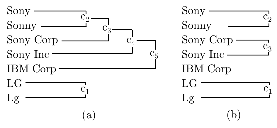
Figure 7. How HAC and HAC with a limit on cluster size work on the same dataset.

Problems with Large Mixed Clusters Produced by HAC:

Using HAC “as is” however does not work well, because it often produces large mixed clusters that are time consuming for user $U$ to clean. Specifically, as HAC iterates, it grows bigger clusters. Initially, when these clusters are small, their quality is often quite good, because they often group together syntactically similar values that refer to the same entity (e.g., “LG” and “Lg”, or “Sony” and “Sonny”, see Figure 7.a).

As the clusters grow, however, they start attracting “junk”, e.g., cluster $c_{4}$ attracts “IBM Corp” (Figure 7.a). If the similarity measure used by HAC happens to be “liberal” for the data set at hand, HAC often grows large clusters that are “mixed”, i.e., containing the values of multiple entities. It is very expensive for user $U$ to clean such clusters, using the Split and Merge procedure described in the previous section.

Proposed Solution:

Ideally, HAC should stop before its clusters become too “mixed”. If HAC’s clusters are smaller but pure (e.g., Figure 8.a), then $U$ mostly just have to merge these clusters using a few mouse clicks. However, if HAC’s clusters are larger but “mixed” (e.g., Figure 8.b), then $U$ would need to split them up into pure clusters, before merging them. This incurs far more mouse clicks and thus far more work.

Of course, we do not know when to stop HAC. To address this problem, we introduce multiple HAC variations, each stopping at a different time, then try to select a good one. Specifically, to cluster $n$ values, we consider $n$ HAC variations, where the $i$-th variation, denoted HAC(i), limits the cluster size to at most $i$. In each iteration, HAC(i) finds the two clusters $c$ and $d$ with the highest similarity score, then merges them if $|c\cup d|\leq i$. Otherwise, HAC(i) finds the two clusters with the next highest score, and merges them if the resulting size is at most $i$, and so on. HAC(i) terminates when it cannot find any more clusters to merge.

Example 4.2.

Consider applying HAC(2) to the values in Figure 7.a. HAC(2) first forms cluster $c_{1}$, then $c_{2}$, exactly as the normal HAC. Then normal HAC goes on to form cluster $c_{3}$ in Figure 7.a, but HAC(2) cannot, because $c_{3}$’s size exceeds 2. Instead, HAC(2) find the next two clusters with the highest similarity score. Suppose these are the singleton clusters for “Sony Corp” and “Sony Inc”. Then HAC(2) merges them to form cluster $c_{3}$ in Figure 7.b. At this point HAC(2) cannot form any more cluster, because any resulting cluster size would exceed 2. So it stops, returning the clusters in Figure 7.b as the output.

HAC(1) produces the smallest but cleanest clusters (as they are singleton). As we increase $i$, HAC(i) tends to produce bigger but less clean clusters. Typically, there exists an i* such that HAC(i*)’s clusters are still so clean that they help user $U$, but HAC(i*+1)’s clusters are already “too dirty” to help (e.g., $U$ would need to split them extensively before her or she can merge). This roughly corresponds to the point where we want HAC to stop. HAC(i*) thus is the “best” HAC variation for the current data set.

To find HAC(i*), we pair HAC(1), $\ldots$, HAC(n) with Split and Merge to form $n$ end-to-end plans. Sections 5 and 6 show how to estimate the costs of these plans and find the one with the least estimated cost.

4.2. Limitations of SM/EM Solutions

We are now in a position to explain why existing string matching (SM) and entity matching (EM) solutions do not work well in our context. (Section 8 shows experimentally that Winston with HAC outperforms these solutions.)

At the core, VN is an SM problem. So SM solutions can be used in the machine part. EM solutions can also be used, by limiting each entity to be a string. Many such solutions have been developed, e.g., TransER (Wang et al., 2013), Magellan (Konda et al., 2016), Falcon (Das et al., 2017), Waldo (Verroios et al., 2017) (see Section 9).

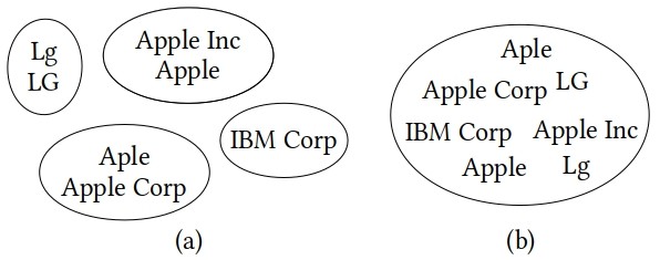
Figure 8. Cleaning (a) is less work than cleaning (b).

These SM/EM solutions (e.g., Magellan, Falcon) typically output a set of matches. One way to use them is to ask user $U$ to verify certain matches, then infer even more matches using match transitivity. For example, given 5 string $a,b,c,d,e$, suppose a solution outputs $a=b$ and $a=c$ as matches. If $U$ has verified these matches, then we can infer $b=c$ as another match. A recent work, TransER (Wang et al., 2013), exemplifies this approach. A serious problem, however, is that we cannot guarantee 100% recall, as shown experimentally in Section 8 For example, no user verification and match transitivity on the outputs $a=b,a=c$ can help us infer $d=e$ (assuming this is also a correct match). Thus, these solutions are not appropriate for Winston.

Another way to use existing SM/EM solutions is to cluster the input strings in a way that respect the output matches. The work (Van Dongen, 2008) describes multiple ways to do this. Continuing with the above example, given the output matches $a=b,a=c$, we can cluster the five input strings into, say, 3 clusters $\{a,b,c\},\{d\},\{e\}$. User $U$ can verify/clean these clusters, as discussed in the human part. A serious problem here, however, is that this approach often produces large mixed clusters, which are very time consuming for $U$ to clean, as shown experimentally in Section 8. With HAC, we solve this problem by modifying HAC to stop early to produce clean clusters (see Section 4.1). But there is no obvious way to modify the clustering algorithms in (Van Dongen, 2008) to stop early such that they produce relatively clean clusters and the quality of these clusters can be estimated (e.g., see Section 5).

The above works provide no GUI, or very basic inefficient GUIs for user feedback, e.g., Falcon and TransER ask users to label string pairs as match/non-match. A recent work, Waldo (Verroios et al., 2017), considers a far more efficient GUI, which displays 6 strings so that a user can cluster all of them in one shot. As such, its “human” part is more similar to ours. But its “machine” part considers a very different optimization problem: namely minimizing crowdsourcing cost (e.g., clustering 6 strings incurs the same monetary cost, regardless of which human user does it). Thus, it cannot be used in Winston, which focuses on minimizing the effort of human users.

5. Estimating Plan Costs

We now discuss estimating the cost of a plan, which is the total time user $U$ spends in the human part to clean the clusters output by the machine part. As we will see below, the key idea is to estimate the quality of these clusters, then use that to estimate the time needed to clean them.

Specifically, let $V=\{v_{1},\ldots,v_{n}\}$ be the set of input values, and $p_{1},\ldots,p_{n}$ be the plans that we will consider, where each plan $p_{\lambda}$ applies HAC($\lambda$) to $V$ to obtain a set of clusters $C_{\lambda}$, then employs a user $U$ to clean $C_{\lambda}$, using Split and Merge. Let $C_{\lambda}=\{c_{1},\ldots,c_{n_{\lambda}}\}$. Then the cost of $p_{\lambda}$ (i.e., the time for $U$ to clean $C_{\lambda}$) can be expressed as $cost(p_{\lambda})=\sum_{i=1}^{n_{\lambda}}time(SplitCluster(c_{i}))\ +\ time(LocalMerge(L))\ +\\ time(GlobalMerge(T)),$ where $L$ is a list of values summarizing the output of SplitCluster, and $T$ is a list summarizing the output of LocalMerge. We now estimate these quantities.

Estimating the Cost of SplitCluster:

We need to estimate $SplitCluster(c_{i})$ for each cluster $c_{i}\in C_{\lambda}$. To do this, we make two assumptions:

(1) All clusters $c_{1},\ldots,c_{n_{\lambda}}$ produced by $p_{\lambda}$ have the same cluster purity $\alpha_{\lambda}$ (which is defined in Definition 3.4).
(2) When we use SplitCluster to split a cluster $c_{i}$ (produced by $p_{\lambda}$) into a pure cluster containing all values of the dominating entity and a “mixed” cluster containing all the remaining values, the “mixed” cluster also has purity $\alpha_{\lambda}$. When we split this “mixed” cluster, the resulting “mixed” cluster also has purity $\alpha_{\lambda}$, and so on.

These are obviously simplifying assumptions. However, they reflect the intuition that each plan HAC($\lambda$) produces clusters of a certain quality level, and that this quality level can be captured by a single number, $\alpha_{\lambda}$, which is the purity of all the clusters. Further, they allow us to efficiently estimate plan costs. Finally, Section 8 empirically shows that with these assumptions we can already find good plans.

Next, we use the above assumptions to estimate the cost of $SplitCluster(c_{i})$. Suppose that we already know $\alpha_{\lambda}$ (we show how to estimate $\alpha_{\lambda}$ later in this section), and that $\alpha_{\lambda}\geq 0.5$, then when splitting $c_{i}$ using SplitCluster, user $U$ creates two clusters: a pure dominating cluster $c_{i,w}$ of size $\alpha_{\lambda}\psi_{i}$, where $\psi_{i}$ is the size of $c_{i}$, and a remainder cluster $c_{i,u}$ of size $(1-\alpha_{\lambda})\psi_{i}$. If $|c_{i,u}|>1$, we assume that its purity is also $\alpha_{\lambda}$. $U$ then splits $c_{i,u}$, etc. After $\beta_{i}$ splits, $U$ has created $\beta_{i}+1$ clusters of sizes $\alpha_{\lambda}\psi_{i},\alpha_{\lambda}(1-\alpha_{\lambda})\psi_{i},\dots,\alpha_{\lambda}(1-\alpha_{\lambda})^{\beta_{i}-1}\psi_{i},(1-\alpha_{\lambda})^{\beta_{i}}\psi_{i}$, such that the last cluster has a single element. Thus we can estimate $\beta_{i}$ as $\lfloor-\log^{\psi_{i}}_{1-\alpha_{\lambda}}\rfloor$. Since we can split a cluster of size $\psi_{i}$ at most $\psi_{i}-1$ times, we set $\beta_{i}=\min(\psi_{i}-1,\lfloor-\log^{\psi_{i}}_{1-\alpha_{\lambda}}\rfloor)$.

Recall that Section 3 defines seven user operations: focus(a), select(a), match(x,y), isPure(c), findDom(c), memorize(v), and recall(v) (see Table 1). Let $\rho_{f},\rho_{s},\rho_{m},\rho_{p},\rho_{d},\rho_{z}$, and $\rho_{r}$ be their costs (i.e., times), respectively. As we will see later, the cost $\rho_{p}$ of isPure(c) is a function of $\psi_{i}$, the size of $c$, and $\alpha_{\lambda}$, the purity of $c$. Hence, abusing notations, we will denote this cost as $\rho_{p}(\psi_{i},\alpha_{\lambda})$ for cluster $c_{i}$. Similarly, the cost $\rho_{d}$ of findDom(c) is a function of the size of $c$, and will be denoted as $\rho_{d}(\psi_{i})$ for cluster $c_{i}$. The remaining five costs (e.g., $\rho_{f},\rho_{s}$, etc.) will be constants. Now we can estimate the cost of $SplitCluster(c_{i})$ where $\alpha_{\lambda}\geq 0.5$ as

$$cost_{SplitCluster}(c_{i};\alpha_{\lambda}\geq 0.5)=\textstyle\sum_{j=1}^{\beta_{i}}[\rho_{p}\big{(}(1-\alpha_{\lambda})^{j-1}\psi_{i},\alpha_{\lambda}\big{)}+\rho_{f}$$

$$+\rho_{s}+\rho_{d}\big{(}(1-\alpha_{\lambda})^{j-1}\psi_{i}\big{)}+\rho_{f}+\rho_{s}+((1-\alpha_{\lambda})^{j-1}\psi_{i})(\rho_{f}+\rho_{m}$$

$$+(1-\alpha_{\lambda})\rho_{s})+\rho_{f}+\rho_{s}].$$

Appendix B discusses deriving the above formula, and computing the cost for the cases $\alpha_{\lambda}\in[0.1,0.5)$ and $\alpha_{\lambda}<0.1$.

Parameter	Meaning	Model	Estimation Method
$\alpha_{\lambda}$	Cluster purity for HAC($\lambda$)	$\alpha_{\lambda}=a\lambda^{b}$	User feedback
$\rho_{f}$	Cost of focus(a)	A constant	Set to 0.5
$\rho_{s}$	Cost of select(a)	A constant	Set to 0.5
$\rho_{m}$	Cost of match(x,y)	A constant	User feedback
$\rho_{p}$	Cost of isPure(c)	$\rho_{p}(\psi,\alpha)=\gamma\psi\alpha+\gamma_{0}$	User feedback
$\rho_{d}$	Cost of findDom(c)	$\rho_{d}(\psi)=\eta_{1}\psi\text{ if }\psi\leq|STM|,$ $\eta_{2}\psi^{2}+\eta_{3}$ o.w.	User feedback
$\rho_{z}$	Cost of memorize(v)	A constant	Set to 0.4
$\rho_{r}$	Cost of recall(v)	A constant	Set to $\rho_{z}$
$\tau$	Shrinkage factor for local merge	A constant	Set to 0.98
$\xi$	Hit factor for global merge	A constant	Set to 0.1

Table 1. Parameters for our cost models.

Estimating the Cost of LocalMerge:

Recall that HAC($\lambda$) produces the set of clusters $C_{\lambda}=\{c_{1},\ldots,c_{n_{\lambda}}\}$, and that $\beta_{i}$ is the total number of splits user $U$ performs in SplitCluster for each cluster $c_{i}$. Then at the end of the split phase, $U$ has produced a set of $r_{\lambda}$ pure clusters, where $r_{\lambda}=\sum_{i=1}^{n_{\lambda}}(\beta_{i}+1)$. Assuming that executing LocalMerge on any list will shrink its size by a factor of $\tau$ (currently set to 0.98), we can estimate the time of executing LocalMerge on the output of the split phase as $r_{\lambda}\rho_{z}+r_{\lambda}(1-\tau)(3\rho_{f}+2\rho_{s})+\rho_{f}+\rho_{s}$ (see Appendix B for an explanation).

Estimating the Cost of GlobalMerge:

LocalMerge produces $r^{\prime}_{\lambda}=\tau r_{\lambda}$ pure clusters to which user $U$ will apply GlobalMerge. Recall that GlobalMerge takes the first three values in the input list $L$, displays them in three columns, then asks $U$ to go through the rest of the values of $L$ and check a box if any value matches the values of the columns (see Figure 6), and so on. We assume that in each such iteration, for each column, $\xi$ values will match, resulting in $\xi$ checkboxes being marked. Then we can estimate the cost of GlobalMege as $\sum_{j=1}^{\left\lfloor 1/(3\xi)\right\rfloor}[3\rho_{z}+(r^{\prime}_{\lambda}-3(j-1)\xi r^{\prime}_{\lambda}-3)\rho_{r}+3(\xi r^{\prime}_{\lambda}-1)(\rho_{f}+\rho_{s})+\rho_{f}+\rho_{s}]$ (see Appendix B).

Estimating the Cluster Purity $\alpha_{\lambda}$:

Recall that we assume all clusters $c_{1},\ldots,c_{n}$ produced by HAC($\lambda$) have the same cluster purity $\alpha_{\lambda}$. Using set-aside datasets, we found that $\alpha_{\lambda}$ could be estimated reasonably well using a power-law function $a\lambda^{b}$ (where $b$ is negative, see Table 1). To estimate $a$ and $b$, we compute $\lambda_{10}$ and $\lambda_{20}$. To compute $\lambda_{10}$, we apply HAC(10) to the set of input values to obtain a set $C_{10}$ of clusters. Next, we randomly sample 3 clusters of size 10 from $C_{10}$ (if there are less than 3 such clusters, we select the three largest). Next, we show each cluster to user $U$, ask him/her to identify all values referring to the dominating entity, then use those to compute the cluster purity. Finally, we take the average purity of these clusters to be $C_{10}$. We proceed similarly to compute $C_{20}$.

We now have three data points: (1,1), (10, $\lambda_{10}$), and (20,$\lambda_{20}$), which we can use to estimate $a$ and $b$ in the function $a\lambda^{b}$, using the ordinary least-squares method.

Estimating the Costs of User Operations:

Finally, we estimate the costs of the seven user operations (see Table 1). The costs of focus(a) and select(a) measure the times user $U$ focuses on an object $a$ then selects it (e.g., by clicking a mouse button). After a number of timing with various users, we found that these times are roughly the same for most users, and we set them to be $\rho_{f}=\rho_{s}=0.5$ seconds. Similarly, we found the times of memorize(v) and recall(v) to be roughly constant, at $\rho_{z}=\rho_{r}=0.4$ seconds respectively (see Table 1).

The time $\rho_{m}$ of match(x,y), however, while largely not dependent on $x$ and $y$, does vary depending on user $U$. Further, estimating the time $\rho_{p}$ of isPure(c) and time $\rho_{d}$ of findDom(c) is significantly more involved. To determine whether a cluster $c$ is pure, user $U$ needs to examine at most $\alpha\psi$ values in $c$ (where $\psi$ is the size of $c$) before he/she sees the first value not referring to $dom(c)$. Hence, we model the time of isPure(c) as $\rho_{p}(\psi,\alpha)=\gamma\,\alpha\,\psi+\gamma_{0}$.

To find the dominating entity $e*$ of cluster $c$, we distinguish two cases. If $\psi\leq|STM|$, then user $U$ can execute findDom(c) entirely in $U$’s short-term memory. In this case the time is proportional to $\psi$. Otherwise $U$ needs to use paper and pen, and we found that the time roughly correlates to $\psi^{2}$. Thus, we model the time $\rho_{d}(\psi)$ of findDom(c) as $\eta_{1}\psi$ if $\psi\leq|STM|$ and as $\eta_{2}\psi^{2}+\eta_{3}$ otherwise.

All that is left is to estimate the cost $\rho_{m}$ of match(x,y), and the parameters $\gamma,\gamma_{0},\eta_{1},\eta_{2},\eta_{3}$ of the cost models of isPure(c) and findDom(c). To do so, when running HAC(20) (to estimate cluster purity $\alpha_{\lambda}$), we also ask user $U$ to perform a few match, isPure, and findDom operations, then use the recorded times to estimate the above quantities (see Appendix B). Altogether, the time it takes for users to calibrate cluster purity $\alpha_{\lambda}$ and the cost models of user operations was mere minutes in our experiments (and was included in the total time of our solution).

6. Searching for the Best Plan

Recall that to cluster the values $V=\{v_{1},\ldots,v_{n}\}$, we consider $n$ plan $p_{1},\ldots,p_{n}$, where each plan $p_{\lambda}$ applies HAC($\lambda$) to $V$ to obtain a set of clusters $C_{\lambda}$, then employs a user $U$ to clean $C_{\lambda}$. We now discuss how to efficiently find the plan $p_{\lambda*}$ with the least estimated cost.

Naively, we can (1) execute HAC($\lambda$) for each plan $p_{\lambda}$ to obtain $C_{\lambda}$, (2) apply the cost estimation procedures in the previous section to $C_{\lambda}$ to compute the cost of $p_{\lambda}$, then (3) return the plan with the lowest cost. Steps 2-3 take negligible times. Step 1 however applies HAC(1), $\cdots$, HAC(n) separately to $V$, which altogether can take a lot of time, e.g., 7.3 minutes for $|V|=480$ and 1.1 hours for $|V|=960$ in our experiments.

To address this problem, we have developed a solution to jointly execute HAC(1), $\cdots$, HAC(n), such that executing a plan can reuse the intermediate results of executing a previous plan. Specifically, we first execute HAC(n), i.e., the regular HAC. Recall that each iteration $Iter_{i}$ of HAC(n) merges two clusters. Let $s(i)$ be the size of the largest cluster at the end of $Iter_{i}$. Suppose there is a $k$ such that $s(i)\leq\lambda$ but $s(i+1)>\lambda$. Then we know that HAC($\lambda$) can reuse everything HAC(n) has produced up to $Iter_{i}$, but cannot proceed to $Iter_{i+1}$. So at the end of $Iter_{i}$ we save certain information for HAC($\lambda$) (e.g., the merge commands so far, the value $\lambda$), then continue with HAC(n). Once HAC(n) is done, we go back to each saved point $\lambda$ and resume HAC($\lambda$) from there. This strategy enables great reuse, especially for high values of $\lambda$, e.g., slashing the time for 960 values from 1.1 hours to 18 secs.

Putting It All Together:

We can now describe the entire Winston system, as used by a single user $U$. Given a set of values $V$ to normalize, (1) Winston first calibrate the cluster purity $\alpha_{\lambda}$ and the cost models. To do so, it runs HAC(10) and HAC(20), asks user $U$ to perform a few basic tasks on sample clusters from these algorithms, then use $U$’s results to calibrate (see Section 5). (2) Winston runs the above search procedure to find a plan $p_{\lambda*}$ with the least estimated cost. (3) Finally, Winston sends the output clusters of $p_{\lambda*}$ to user $U$ to clean, using procedures Split and Merge.

7. Working with Multiple Users

So far we have discussed how Winston works with a single user. In practice, however, multiple users (e.g., people in the same team) are often willing to jointly perform VN. We now discuss how to extend Winston to divide the work among such users, to speed up VN.

Consider the case of 3 users. Naively, we can divide the set of input strings into 3 equal parts, ask each user to apply Winston to perform VN for a part, then combine the three outputs to form a set of clusters. We can obtain a canonical string from each cluster, producing a new list of strings. Then we can divide this new list among 3 users, repeat the process, and so on. This naive solution however does not work well, because it often spreads matching strings, i.e., those belonging to a golden cluster, among all 3 users, causing much additional work in matching across the individual lists, in later steps.

Intuitively, strings within a golden cluster should be assigned to a single user, as much as possible. We have extended Winston to realize this intuition. In the extension, Winston first briefly interacts with each user to learn his/her profiles. Next, it uses these profiles to search a plan space to find a good VN plan. Next, it executes the machine part of this plan to produce a set $C$ of clusters. It then divides $C$ among the users, such that each will have roughly the same workload. The intuition here is that a cluster in $C$ captures many strings that belong to the same golden cluster, and is assigned to a single user. Next, Winston asks each user to use Split and Merge to clean the assigned clusters. Finally, it obtains the set of (cleaned) clusters from all users, then repeatedly performs a distributed version of GlobalMerge until all clusters have been verified and cleaned. Appendix C describes the algorithm in detail, provides the pseudo code, and discusses cost estimation procedures for this version of Winston.

8. Empirical Evaluation

We now evaluate Winston. Among others, we show that Winston can significantly outperform existing solutions, that it can leverage multiple users to drastically cut VN time, and that it can scale to large datasets.

Name	Size	Description	Sample Values
Nickname	5132	Nicknames and some of their typos	“Cissy”, “Fanny”, “Frannie”
Citation	3000	Article citations from Google Scholar and DBLP	“caching technologies for web applications c mohan vldb 2001”
Life Stage	199	Target life stage(s) of products	“Maternity”, “Mothers”, “Youth| Young Professionals”
Big Ten	74	Names of Big Ten Conference colleges	“University of Iowa”, “UIowa”, “UM Twin Cities”

Table 2. Datasets for our experiments.

8.1. Existing Manual/Clustering Solutions

We first compare Winston with state-of-the-art manual and clustering solutions (Section 8.3 considers string/entity matching solutions). We use the four datasets in Table 2, obtained online and from VN tasks at a company. For each dataset we manually created all correct clusters, to serve as the ground truth. (We consider larger datasets later in Section 8.4.)

The Existing Solutions:

We consider four solutions: Manual, Merge, Quack, and OpenRefine. Manual is the typical manual method that we have observed in industry. It can be viewed as performing the GlobalMerge method (Section 3.2). Merge is our own manual VN method, which performs LocalMerge then GlobalMerge.

Quack is a string clustering tool used extensively for VN at a company. It also uses HAC like Winston, but does not place a limit on the cluster size. We extended Quack by asking the user to clean the clusters using Split and Merge. Merge and Quack can be viewed as the two plans HAC(1) and HAC($n$) in the plan space explored by Winston (where $n$ is the number of values to be normalized).

OpenRefine is a popular open-source tool to wrangle data (ope, 2018). It uses several string clustering algorithms to perform VN (orc, 2018). Among these, the most effective one appears to be KNN-based clustering (orc, 2018). We extend this algorithm to work with Split and Merge (because the GUI provided by OpenRefine is very limited).

Results:

Table 3 shows the times of Winston vs. the above four methods (in minutes), using a single user. For each method we measure the total time the user spends cleaning the clusters (for Winston this includes the calibration time). It is difficult to recruit a large number of real users for these experiments, because cleaning some datasets (e.g., Nickname) would take a few working days. So we use synthetic users and each data point here is averaged over 100 such users, see Appendix D. (We use real users to “sanity check” these results in Section 8.4.)

The table shows that Manual performs worst, incurring 3-6800 minutes. Merge performs much better, especially on the two large datasets, incurring 4-1961 minutes, suggesting that performing a local merge before a global merge is important. Merge is clearly the manual method to beat.

Quack is a bit faster than Merge on Nickname (1808 vs. 1961), but slower on the remaining three datasets. OpenRefine’s performance is very uneven. It is a bit faster than Merge on Citation, but far slower on the other three datasets.

In contrast, Winston performs much better than Merge. On Nickname it saves 7.5 hours of user time (see the last column). On Citation it saves 3.34 hours of user time. On Life Stage it is comparable to Merge, and on Big Ten it is only 3 mins worse (due to the overhead of user calibration time).

Winston also outperforms both Quack and OpenRefine. Importantly, in all cases where Quack or OpenRefine performs worse than Merge, Winston is able to select a good plan which allows it to outperform Merge.

Dataset	Manual	Merge	Quack	OpenRefine	Winston	Savings
Nickname	6800	1961	1808	$>$10000	1512	7.5hrs
Citation	6585	1313	1371	1280	1112	3.4hrs
Life Stage	13	9	15	12	9	0hrs
Big Ten	3	4	9	22	7	-3min

Table 3. Winston vs four existing solutions.

Dataset	1 User	3 Users	5 Users	7 Users	9 Users
Nickname	1512	890	610	460	412
Citation	1112	428	278	212	177
Life Stage	9	6	6	6	6
Big Ten	7	4	4	4	4

Table 4. The times of Winston with multiple users.

8.2. Working with Multiple Users

We have shown that Winston outperforms existing manual and clustering methods. We now examine how Winston can leverage multiple users to reduce VN time. Table 4 shows that Winston can leverage multiple users to drastically cut the VN time, e.g., from 1512 minutes with 1 user to 412 with 9 users for Nickname, and from 1112 to 177 for Citation. The most significant reduction is achieved early, e.g., from 1 to 3-5 users. After that, adding more users still helps reduce the VN time, but only in a “diminishing-return” fashion.

8.3. Limitations of SM/EM Solutions

We now compare Winston to existing string matching (SM) and entity matching (EM) solutions, specifically with TransER (Wang et al., 2013), Falcon (Das et al., 2017), and Magellan (Konda et al., 2016).

Comparing with TransER:

As discussed in Section 4.2, there are two main ways to use SM/EM solutions in our context. First, a solution can produce a set of matches $M$, employ a user $U$ to verify certain matches in $M$, then use match transitivity to infer even more matches. The work (Wang et al., 2013) describes such a solution, which we call TransER.

The main problem, as discussed in Section 4.2, is that such solutions cannot guarantee 100% recall. Consider TransER, which matches strings using rule $Jaccard(3g(v_{i}),3g(v_{j}))\geq\alpha$. Assuming a perfect user $U$ who does not make mistakes when verifying matches, Figure 9 shows the recall of TransER on our four datasets as we vary $\alpha$. It shows that to reach 100% recall, $\alpha$ must be set to less than 0.08. But that would produce a huge number of matches (almost the entire Cartesian product), which require a huge amount of effort from the user to verify. In such cases, it is not difficult to show that TransER would perform worse than Merge.

Comparing with Falcon and Magellan:

The second way to use current SM/EM solutions is to produce the matches, then group them into clusters. To examine this approach, we use Falcon (Das et al., 2017) and Magellan (Konda et al., 2016). A recent work (name withheld for anonymous reviewing) has adapted Falcon to SM, and shown that it outperforms existing SM solutions. Thus, Falcon can be viewed as a state-of-the-art SM solution. Magellan, on the other hand, can be viewed as a state-of-the-art EM solution. To learn a matcher, both Falcon and Magellan require the user to label a set of pairs as match/non-match. In Magellan the user can also debug the matcher to improve its accuracy.

Once Falcon and Magellan have produced the matches, we use Markov clustering in (Van Dongen, 2008) to partition the input strings into clusters that are consistent with the matches. Finally, we ask one or more users to clean the clusters using Split and Merge.

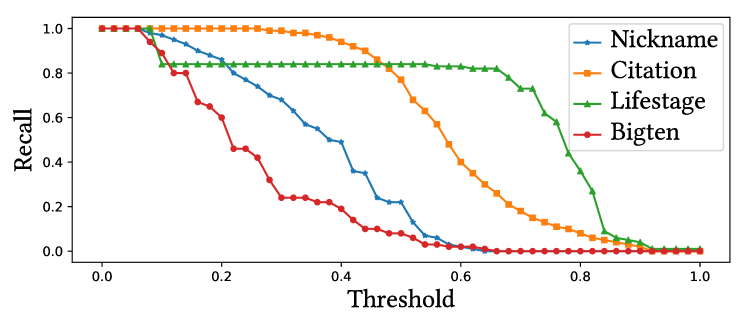
Figure 9. Recall of TransER for varying threshold $\alpha$.

Dataset	1 User	3 Users	5 Users	7 Users	9 Users	Labeling
Nickname	1930 ( 418)	1519 ( 629)	1210 ( 600)	958 ( 498)	807 ( 395)	14
Citation	1114 ( 2)	1302 ( 874)	779 ( 501)	562 ( 350)	459 ( 282)	19
Life Stage	22 ( 13)	21 ( 15)	21 ( 15)	22 ( 16)	22 ( 16)	20
Big Ten	21 ( 14)	21 ( 17)	21 ( 17)	21 ( 17)	21 ( 17)	20

Table 5. The human times of Falcon.

Dataset	1 User	3 Users	5 Users	7 Users	9 Users	Labeling & Debugging
Nickname	1482 ( -30)	1062 ( 172)	788 ( 178)	646 ( 186)	563 ( 151)	89
Citation	1150 ( 38)	900 ( 472)	599 ( 321)	481 ( 269)	393 ( 216)	109
Life Stage	85 ( 76)	85 ( 79)	85 ( 79)	85 ( 79)	85 ( 79)	84
Big Ten	85 ( 78)	85 ( 81)	85 ( 81)	85 ( 81)	85 ( 81)	84

Table 6. The human times of Magellan.

Table 5 shows the human time for Falcon on the four datasets. For example, the first cell “1930 (418)” means that for 1 user, Falcon incurs 1930 mins of human time, 418 mins more than Winston. This time includes the labeling time (14 mins, shown in the last column). The table shows that Winston outperforms Falcon in all cases, reducing human time by 2-874 mins. The larger the dataset, the more the gain, e.g., more than 14.5 hours on Citation, using 3 users.

Table 6 shows the human time for Magellan on the four datasets. The meaning of the table cells here are similar to those for Falcon. The table shows that Winston outperforms Magellan in all cases, reducing human time by 38-472 mins, except in the case of 1 user for Nickname, where it is slower by 30 mins (see the red font).

The above time includes labeling and debugging (the last column). Interestingly, even if we ignore the labeling and debugging time, Winston still outperforms Magellan by a large margin in all cases requiring 3, 5, 7, and 9 users, for Nickname and Citation. It is slower only in the case of 1 user, by 119 mins for Nickname and 71 mins for Citation. Thus, overall Winston outperforms Magellan. In addition, Winston is suitable for lay users, whereas Magellan requires the user to have expertise in EM and machine learning.

A major reason for the worse performance of Falcon and Magellan is that they often produce large mixed clusters. For example, Magellan produces clusters of up to 314 strings coming from 137 real-world entities on Nickname, and clusters of up to 98 strings coming from 62 real-world entities on Citation. Clearly, it is very time consuming for the user to clean such clusters. In contrast, Winston selects VN plans that produce clusters of only up to 20 strings, which are much easier for the user to understand and clean.

8.4. Additional Experiments

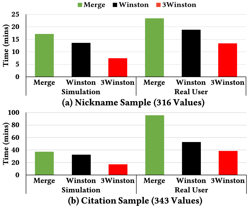
Figure 10. “Sanity check” with real users.

“Sanity Check” with Real Users:

We want to “sanity check” our results so far using real users. Extensive checking is very difficult because it is hard to recruit real users for these time-consuming experiments. As a result, we carried out a limited checking. Specifically, we performed stratified sampling to obtain a Nickname sample of 316 values and a Citation sample of 343 values. On each sample we recruited multiple real users and asked them to perform Merge, Winston and 3Winston (i.e., Winston with 3 users), taking care to minimize user bias. The right side of Figure 10.a shows the results for Nickname. For comparison purposes, the left side of the figure shows the times with synthetic users. Figure 10.b shows similar results for Citation.

The figures show that “Simulation” approximates “Real User” quite well. In both cases, the ordering of the methods is the same. Further, the results show that Winston can do much better than Merge, and 3Winston in turn can do much better than Winston. While limited, this result with real users does provide some anecdotal support for our simulation findings.

Finding Good Plans:

Table 7 shows that Winston finds good plans. Consider Nickname. Recall that we ran 100 synthetic users for this dataset. For each user $U_{i}$ Winston estimated the costs of all plans then selected plan $p+$, the one with the least estimated cost. Knowing gold clusters, however, we can simulate how $U_{i}$ executes each plan and thus compute the plan’s exact cost. This allows us to find the rank of $p+$ on the list of all plans sorted by increasing cost, as well as the time difference between $p+$ and the best plan.

The first row of Table 7 shows this information. Here, Winston considered a space of 100 plans. For all 100 users, it selected the plan ranked 2nd. The difference between this plan and the best plan, however, is just 3-4 mins (over 100 users). The next two cells show the average/min/max times of the best plan, and the average/min/max difference in percentage. The remaining rows are similar. Thus, Winston did a good job. In many cases, it selected top-ranked plans, and most importantly, all the selected plans differ in time from the best plans by only 0-14% (see the last column).

Scaling to Large Datasets:

Finally, we examine how Winston scales to large datasets. Table 8 shows the estimated cleaning time of Merge, Quack, Winston, and 3Winston, i.e., Winston with 3 users, for synthetic datasets of various sizes. The table shows that Merge is not practical, taking 29 days, 4.4 years, and 11.5 years for 100K, 500K, and 1M strings, respectively. Quack is better, but still incurs huge times.

Winston, in contrast, can reduce these times drastically, to just 13 days, 9.6 months, and 1.3 years, respectively. As discussed in Section 1, this is because Winston provides a better UI, so the user can do more with less effort. Further, the machine part of Winston outputs clusters that are “user friendly”, i.e., requiring little effort for the user to clean. Finally, Winston searches a large space of plans to find one with minimal estimated human effort. 3Winston does even better, cutting the times to clean 500K and 1M strings to just 2.2 and 3.5 months, respectively. These suggest that cleaning large datasets with Winston indeed can be practical, especially by dividing the work among multiple users.

Dataset	Picked Plan Rank (Freq)	Size of Plan Space	Time Diff to Best Plan	Time of Best Plan	Diff in %
Nickname	2 (100)	100	(3,4)	2007 (1557,2451)	0.1 (0.1,0.2)
Citation	1 (100)	100	(0,0)	1251 (975,1567)	0 (0,0)
Life Stage	5 (5), 7 (19), 9 (76)	100	(0.5,0.7)	8.1 (7.2,9.2)	7 (6,8)
Big Ten	2 (73)	73	(0.6,1.2)	5.3 (5,5.7)	14 (9,18)

Table 7. The quality of the plans found by Winston.

Dataset Size	Merge	Quack	Winston	3Winston
10K	22	22	13	4
100K	231 ( 29d)	199	107 ( 13d)	34 ( 4.2d)
500K	9415 ( 4.4y)	3231	1688 ( 9.6m)	387 ( 2.2m)
1M	24449 ( 11.5y)	19971	2710 ( 1.3y)	618 ( 3.5m)

Table 8. Cleaning times vs dataset sizes.

9. Related Work

Data Cleaning:

Data cleaning has received enormous attention (e.g., (Galhardas et al., 2001; Khayyat et al., 2015; Haas et al., 2015; Efthymiou et al., 2015; Das Sarma et al., 2012; Chu et al., 2016b; Kolb et al., 2011; Mozafari et al., 2014; Parameswaran and Polyzotis, 2011; Marcus et al., 2011; Park and Widom, 2013; Haas et al., 2016; Franklin et al., 2011; Wang et al., 2013; Krishnan et al., 2016; Heer et al., 2015; Abedjan et al., 2016; Dong et al., 2010; Freire et al., 2016; Arasu et al., 2011; Chaudhuri et al., 2006)). See (Chu et al., 2016a; Chu and Ilyas, 2016; Dasu and Johnson, 2003; Rahm and Do, 2000) for recent tutorials, surveys, and books. However, as far as we can tell, no published work has examined the problem of cleaning with 100% accuracy, as we do for VN in this paper. Our work here shows that the problem of cleaning to reach a desired level of accuracy raises many novel challenges for data cleaning.

Value Normalization:

Much work has addressed VN, typically under the name “synonym discovery”. Most solutions use string/contextual similarities to measure the relatedness of values (Yates and Etzioni, 2009; Chakrabarti et al., 2012), and employ various techniques, e.g., clustering, regular expressions, learning, etc. (McCrae and Collier, 2008; Yates and Etzioni, 2009) to match values. However, no work has examined verifying and cleaning VN results to reach 100% accuracy, as we do here.

Clustering:

Our work is related to clustering (which we use in VN). Numerous clustering algorithms exist (Jain et al., 1999; Xu and Wunsch, 2005; Fahad et al., 2014), but we are not aware of any work that has developed a human-driven procedure to clean up clustering output and tried to minimize the human effort of this procedure. Much work has also tuned clustering (e.g., (Basu et al., 2002; Bilenko et al., 2004)), but for accuracy. In contrast, our work can be viewed as tuning clustering to minimize the post-clustering cleaning effort.

String/Entity Matching for the “Machine” Part:

At the core VN is a matching problem, and hence string matching (SM) and entity matching (EM) solutions can be used in the “machine” part. Numerous such solutions have been developed (e.g., TransER, Falcon, Magellan, Waldo and more (Wang et al., 2013; Das et al., 2017; Konda et al., 2016; Verroios et al., 2017)). We have discussed in Section 4.2 and experimentally validated in Section 8.3 that these methods do not work well for our context. The main reason is that they generate large mixed clusters that are very time consuming for users to clean. This result suggests that when we combine a machine part with a human part, it is important to develop the machine part such that it generates results that are “user friendly” for the user in the human part to work with.

User Interaction Techniques for the “Human” Part:

Many recent works on string/entity matching and crowdsourcing solicit user feedback/action via GUIs to verify and further clean (e.g., CrowdDB, CrowdER, and more (Franklin et al., 2011; Wang et al., 2012, 2013; Firmani et al., 2016; Verroios and Garcia-Molina, 2015; Verroios et al., 2017)). These works however allow only a limited range of user actions (e.g., asking users if two tuples match). A recent work, Waldo (Verroios et al., 2017), considers more expressive user actions, such as showing six values on a single screen and allowing the user to cluster all six in “one shot”. The above works differ from Winston in two important ways. First, the range of user actions that they allow is still quite limited. In contrast, Winston considers far more expressive user actions, such splitting a cluster, merging two clusters, etc. Second, the above works do not explicitly model the human effort of the user actions and do not seek to minimize this total human effort, as Winston does. For example, they model the cost of labeling a value pair or clustering six values to be a fixed value (e.g., 3 cents paid to a crowd worker), regardless of how much effort a user puts into doing it. As such, our work can be viewed as advancing the recent human-in-the-loop (HILDA) line of research, by considering more expressive user actions and studying how to optimize their human-effort cost using RDBMS-style techniques.

RDBMS-Style Cleaning Systems:

Many cleaning works have also adopted an RDBMS-style operator framework, e.g., AJAX (Galhardas et al., 2001), Wisteria (Haas et al., 2015), Arnold (Jeffery et al., 2013), QuERy (Altwaijry et al., 2015). They however do not consider expressive human operations, modeling human actions at a coarse level, e.g, labeling a tuple, converting a dirty tuple into a clean one. In contrast, we model and estimate the cost of complex human operations, e.g., removing a value from a cluster, verifying if a cluster is clean, etc. Finally, current work typically optimizes for the accuracy and time of cleaning algorithms (while assuming a ceiling on the human effort). In contrast, we minimize the human effort, which can be a major bottleneck in practice.

Interactive Cleaning Systems:

Another prominent body of work develops interactive cleaning systems (e.g., AJAX (Galhardas et al., 2001), Potter Wheel (Raman and Hellerstein, 2001), Wrangler (Kandel et al., 2011), Trifacta (Heer et al., 2015), ALIAS (Sarawagi et al., 2002), and (He et al., 2016). Such systems often try to maximize cleaning accuracy, or efficiently build data transformations/cleaning scripts, while minimizing the user effort. To the best of our knowledge, however, they have not examined the problem of VN with 100% accuracy. For example, active learning-based approaches such as (Sarawagi et al., 2002) do not tell the user what to do (to reach 100% accuracy) if after using them the accuracy of the cleaned dataset is still below 100%.

10. Conclusions & Future Work

We have examined the problem of value normalization with 100% accuracy. We have described Winston, an RDBMS-style solution that defines human operations, combines them with clustering algorithms to form hybrid plans, estimates plan costs (in terms of human verification and cleaning effort), then selects the best plan.

Overall, our work here shows that it is indeed possible to apply an RDBMS-style solution approach to the problems of 100% accurate cleaning. Going forward, we plan to open source our current VN solution, explore other clustering algorithms for VN, and explore applying the solutions here to other cleaning tasks, such as deduplication, outlier removal, extraction, and data repair.

Appendix A Defining the Human Part

Algorithm LABEL:algo:globalmerging describes the Merge and GlobalMerge procedures (LocalMerge has been described in Section 3.2).

Appendix B Estimating Plan Costs

In this section we describe the cost estimation formula for various procedures used in the human part of value normalization plans and how we have derived them.

SplitCluster Procedure:

To estimate the cost of applying SplitCluster  to a cluster $c_{i}$ during the execution of the plan $p_{\lambda}$ we consider the following three cases:

Case 1 ($\alpha_{\lambda}\geq 0.5$): Recall that when $\alpha_{\lambda}\geq 0.5$ we estimate the cost of applying SplitCluster  to $c_{i}$ as follows:

$$cost_{SplitCluster}(c_{i};\alpha_{\lambda}\geq 0.5)=$$

$$\sum_{j=1}^{\beta_{i}}[\underbrace{\rho_{p}\big{(}(1-\alpha_{\lambda})^{j-1}\psi_{i},\alpha_{\lambda}\big{)}+\rho_{f}+\rho_{s}}_{q_{1}}+\underbrace{\rho_{d}\big{(}(1-\alpha_{\lambda})^{j-1}\psi_{i}\big{)}+\rho_{f}+\rho_{s}}_{q_{2}}$$

$$+\underbrace{((1-\alpha_{\lambda})^{j-1}\psi_{i})(\rho_{f}+\rho_{m}+(1-\alpha_{\lambda})\rho_{s})}_{q_{3,1}}+\underbrace{\rho_{f}+\rho_{s}}_{q_{3,2}}]$$

Also recall that we go through $\beta_{i}$ iterations of splitting $c_{i}$ and at iteration $j\in\{1,\dots,\beta_{i}\}$ we split an impure cluster of approximate size $(1-\alpha_{\lambda})^{j-1}\psi_{i}$, e.g. at iteration 1 we split the whole cluster of size $(1-\alpha_{\lambda})^{0}\psi_{i}=\psi_{i}$. Each iteration corresponds to a (recursive) call of the SplitCluster. At each execution of SplitCluster, there are three lines (numbered 2, 4 and 7 in Algorithm 1) involving user operations and thus only these lines contribute to the cost of the procedure.

The cost of line 2 is captured by part $q_{1}$ of the above formula: it consists of the cost of isPure (executed on a cluster of size $(1-\alpha_{\lambda})^{j-1}\psi_{i}$) and then focusing on and selecting “no" button. Part $q_{2}$ captures the cost of line 4: it consists of the cost of findDom and then focusing on and selecting “mark values" button. Finally parts $q_{3,1}$ and $q_{3,2}$ of the above formula capture the cost of line 7: $q_{3,1}$ is the cost of MarkValues and $q_{3,2}$ is the cost of focusing on and selecting “create/clean new cluster" button. Part $q_{3,1}$ in turn consists of going through the cluster values (line 3 in MarkValues pseudo code), focusing on each value, matching it with the dominating entity of the cluster and selecting the value if they match (i.e. for $1-\alpha_{\lambda}$ fraction of the values).

Case 2 ($\alpha_{\lambda}\in[0.1,0.5)$): We estimate the cost of applying SplitCluster  to $c_{i}$ when $\alpha_{\lambda}\in[0.1,0.5)$ as follows:

$$cost_{SplitCluster}(c_{i};\alpha_{\lambda}\in[0.1,0.5))=\textstyle\sum_{j=1}^{\beta_{i}}[\rho_{p}\big{(}(1-\alpha_{\lambda})^{j-1}\psi_{i},\alpha_{\lambda}\big{)}$$

$$+\rho_{f}+\rho_{s}+\rho_{d}\big{(}(1-\alpha_{\lambda})^{j-1}\psi_{i}\big{)}+\rho_{f}+\rho_{s}+((1-\alpha_{\lambda})^{j-1}\psi_{i})(\rho_{f}$$

$$+\rho_{m}+\alpha_{\lambda}\rho_{s})+\rho_{f}+\rho_{s}].$$

The derivation is very similar to the previous case. The only difference is the fraction of matching values at each execution of MarkValues which is $\alpha_{\lambda}$ instead of $1-\alpha_{\lambda}$.

Case 3 ($\alpha_{\lambda}<0.1$): When $\alpha_{\lambda}<0.1$ we estimate the cost of applying SplitCluster  to $c_{i}$ as follows:

$$cost_{SplitCluster}(c_{i};\alpha_{\lambda}<0.1)=\underbrace{\rho_{p}\big{(}\psi_{i},\alpha_{\lambda}\big{)}+\rho_{f}+\rho_{s}}_{q^{\prime}_{1}}$$

$$+\underbrace{\rho_{d}\big{(}\psi_{i}\big{)}+\rho_{f}+\rho_{s}}_{q^{\prime}_{2}}+\underbrace{\psi_{i}\rho_{z}+\psi_{i}(1-\tau)(3\rho_{f}+2\rho_{s})+\rho_{f}+\rho_{s}}_{q^{\prime}_{3}}$$

$$+\textstyle\sum_{j=1}^{\beta_{i}}[3\rho_{z}+(3(1-\alpha_{\lambda})^{3(j-1)}\tau\psi_{i}-3)\rho_{r}$$

$$+(\textstyle\sum_{k=1}^{3}\alpha_{\lambda}(1-\alpha_{\lambda})^{3(j-1)+k}\tau\psi_{i}-1)(\rho_{f}+\rho_{s})+\rho_{f}+\rho_{s}]$$

Here $q^{\prime}_{1}$ is the cost of executing isPure on $c_{i}$ and then focusing on and selecting “no" button. $q^{\prime}_{2}$ is the cost of executing findDom and then focusing on and selecting “clean mixed cluster" button. $q^{\prime}_{3}$ is the cost of executing LocalMerge  on $c_{i}$ and the rest of the formula is the cost of executing GlobalMerge   on the results of the previous step. We will describe the costs of LocalMerge  and GlobalMerge  in the following sections.

LocalMerge Procedure:

Recall that for a particular plan $p_{\lambda}$ the split phase result consists of approximately $r_{\lambda}$ pure clusters of input values. Thus the size of the input list $L$ to the LocalMerge  is $r_{\lambda}$. User $U$ goes through the values in $L$ and for each value, he or she first memorizes it. For $1-\tau$ fraction of the values in $L$, $U$ finds a value in his or her short-term memory (STM) in which case he or she (1) selects the current value, then focuses on and selects the value retrieved from STM and finally focuses on and selects the link button. Finally the user focuses on and selects “done local merging” button to proceed to the global merging. Adding up these costs gives us the cost formula $r_{\lambda}\rho_{z}+r_{\lambda}(1-\tau)(3\rho_{f}+2\rho_{s})+\rho_{f}+\rho_{s}$.

GlobalMerge Procedure:

GlobalMerge takes as input a list of values $L$ with approximate size $r^{\prime}_{\lambda}$. The GlobalMerge consists of possibly several iterations and in each iteration, we assume that each of the three values displayed on the columns of the GUI would match approximately $\xi r^{\prime}_{\lambda}-1$ values displayed on the rows, forming clusters of size $\xi r^{\prime}_{\lambda}$. Thus the number of iterations of GlobalMerge  would be approximately $g_{\lambda}=\left\lfloor r^{\prime}_{\lambda}/(3\xi r^{\prime}_{\lambda})\right\rfloor=\left\lfloor 1/(3\xi)\right\rfloor$.

At iteration $j\in\{1,\dots,g_{\lambda}\}$ the user sees $r^{\prime}_{\lambda}-3(j-1)\xi r^{\prime}_{\lambda}$ values remained to be matched, three of which are displayed on the columns and the rest on the rows of the GUI. The user first memorizes the three values on the columns (with total cost of $3\rho_{z}$). Then for the $r^{\prime}_{\lambda}-3(j-1)\xi r^{\prime}_{\lambda}-3$ values on the rows the user recalls each value. Lastly for each of the three columns the user focuses on and selects checkboxes for $\xi r^{\prime}_{\lambda}-1$ rows. Finally the user focuses on and selects “global merge” button to finish the current round. Adding up these costs would give us the cost formula $\sum_{j=1}^{\left\lfloor 1/(3\xi)\right\rfloor}[3\rho_{z}+(r^{\prime}_{\lambda}-3(j-1)\xi r^{\prime}_{\lambda}-3)\rho_{r}+3(\xi r^{\prime}_{\lambda}-1)(\rho_{f}+\rho_{s})+\rho_{f}+\rho_{s}]$

Estimating the Costs of User Operations:

We now describe how we estimate the cost $\rho_{m}$ of the match operation, the parameters $\gamma$ and $\gamma_{0}$ of the isPure operation cost function and the parameters $\eta_{1},\eta_{2}$ and $\eta_{3}$ of the findDom operation cost function during the calibration stage.

To estimate $\rho_{m}$ we first pick three pairs of random values of $V$. We then ask the user $U$ to match each pair and, depending on whether they match or not, to selects a “yes” or “no” button. For the $k$th pair we measure the time $t_{m,k}$ it takes from when we show the screen containing the pair of values and the buttons to $U$ till he or she selects one of the buttons. During this time the user matches the values shown on the screen, then focuses on one of the buttons and selects it. Hence the time we measure is equal to $\rho_{m,k}+\rho_{f}+\rho_{s}$ where $\rho_{m,k}$ is our estimated cost of the $k$th match operation. We then calculate the $\rho_{m,k}=t_{m,k}-(\rho_{f}+\rho_{s})$ and estimate $\rho_{m}$ to be the average of $\rho_{m,k}$s, i.e. $\rho_{m}=\sum_{k=1}^{3}\rho_{m,k}/3$.

For the rest of the parameters above we use the results of HAC(20) we have previously run on the input dataset during the calibration phase. Denote the results of HAC(20) as $C_{20}$. First we pick three random non-singleton clusters $c_{1}$, $c_{2}$ and $c_{3}$ (of different sizes if possible) from $C_{20}$. Then we show each $c_{k}$ and ask $U$ to select a “yes” button if $c_{k}$ is pure and a “no” button otherwise. We record the time $t_{p,k}$ it takes from when we show $c_{k}$ to $U$ till one of the buttons is selected. We also record which button is selected. Using the same timing analysis we described for $\rho_{m}$, we form three equations of the form $\gamma\alpha(c_{k})\psi_{k}+\gamma_{0}=t_{p,k}-(\rho_{f}+\rho_{s})$ where $k\in\{1,2,3\}$, $\alpha(c_{k})$ is the purity of $c_{k}$ and $\psi_{k}$ is the size of $c_{k}$. However since we don’t know the purity of $c_{k}$s, we use the button $U$ has selected to guess the purity of $c_{k}$: if $U$ has selected the “yes” button, we set $\alpha(c_{k})=1$, otherwise we set $\alpha(c_{k})=a(20)^{b}$ (we have already estimated $a$ and $b$ during the calibration of the purity function). Finally we use ordinary least-squares method to solve the system of three equations above to estimate the parameters $\gamma$ and $\gamma_{0}$.

To estimate $\eta_{1}$ we first pick three clusters $c^{\prime}_{1}$, $c^{\prime}_{2}$ and $c^{\prime}_{3}$ from $C_{20}$ such that $\psi^{\prime}_{k}=|c^{\prime}_{k}|\leq|STM|$. We then show each $c^{\prime}_{k}$ to $U$ and ask him/her to find the dominating entity of $c^{\prime}_{k}$, and then select a value in $c^{\prime}_{k}$ which refers to dom($c^{\prime}_{k}$). For each $c^{\prime}_{k}$ we measure the time $t_{\eta_{1},k}$ it takes from when it is shown to $U$ till he/she selects the value referring to dom($c^{\prime}_{k}$). Using the same timing analysis as above we obtain three equations of the form $t_{\eta_{1},k}=\eta_{1}\psi^{\prime}_{k}+\rho_{f}+\rho_{s}$. Then we solve each equation for $\eta_{1}$ and finally average the three numbers we get to estimate $\eta_{1}$ as $\sum_{k=1}^{3}(t_{\eta_{1},k}-(\rho_{f}+\rho_{s}))/\psi^{\prime}_{k}$.

To estimate $\eta_{2}$ and $\eta_{3}$ we follow a similar process: we first pick three clusters $c^{\prime\prime}_{1}$, $c^{\prime\prime}_{2}$ and $c^{\prime\prime}_{3}$ from $C_{20}$ such that $\psi^{\prime\prime}_{k}=|c^{\prime\prime}_{k}|>|STM|$. We then show each $c^{\prime\prime}_{k}$ to $U$ and ask him/her to find the dominating entity of $c^{\prime\prime}_{k}$ and then select a value in $c^{\prime\prime}_{k}$ which refers to dom($c^{\prime\prime}_{k}$). For each $c^{\prime\prime}_{k}$ we measure the time $t_{\eta_{2,3},k}$ it takes from when it is shown to $U$ till he/she selects the value referring to dom($c^{\prime\prime}_{k}$). Using the same timing analysis as above we obtain three equations of the form $t_{\eta_{2,3},k}=\eta_{2}(\psi^{\prime\prime}_{k})^{2}+\eta_{3}+\rho_{f}+\rho_{s}$. Finally we use ordinary least-squares method to solve the system of three equations above to estimate the parameters $\eta_{2}$ and $\eta_{3}$.

Appendix C Working with Multiple Users

We now describe cWinston, which extends Winston to work with multiple users. Assuming $k$ users want to collaborate to normalize a set $V$ of input values, cWinston goes through four main stages. In the first stage, it shows each user a few clusters of values in $V$ and asks them to perform some basic operations on them. cWinston then uses the results of these operations to tune the purity function parameters and user operation cost models for each user (the same way as Winston). Next, it takes the average of purity function and cost model parameters to create a single purity function and a single cost model for each user operation.

In the second stage, cWinston uses the above purity function and user operation cost models to find the best VN plan. To do so, it uses the same plan space searching procedure as Winston (see Section 6) to find the best plan. It then executes the machine part of the best plan to obtain a set $\mathcal{C}$ of clusters.

In the third stage, cWinston partitions $\mathcal{C}$ into $k$ subsets of roughly the same number of values. It then assigns each subset to one of the users and asks them to clean their respective subsets of clusters using Split and Merge algorithms.

In the last stage, cWinston starts by collecting the results of Split+Merge from all the users and for each user, it creates a list of representative values of the clean clusters he or she has produced. It then picks the longest list and divides it into $k$ chunks of roughly the same size. Next, cWinston asks each user to merge one of these chunks with the rest of the lists using the GlobalMerge procedure (see Section 6). It then collects the results from all the users and repeats this stage (i.e., takes representative values from the merged clusters, divides the largest list into $k$ chunks, and so on) until all of the lists are verified/merged. Algorithm 4 shows the pseudocode of cWinston.

Estimating the Cost of cWinston:

Next, we describe how we estimate the cost of cWinston. To do so, we traverse Algorithm 4, using the same assumption as we discussed in Section 5, to arrive at the following cost formula:

$$cost_{{\sf cWinston}}{=} \max_{1\leq i\leq k}\Big{(}cost_{{\sf Split},u_{i}}(C_{i}^{\prime}){+}cost_{{\sf LocalMerge},u_{i}}(E_{i}){+}cost_{{\sf GlobalMerge},u_{i}}(L_{i})\Big{)}$$

$$+ cost_{\text{MultiUserMerge},U}(S)$$

where $k$ is the number of users, the $\max$ term finds the longest it takes any of the users $u_{i}$s to perform Split+Merge on their respective partitions, and the last term is the cost of multi-user merge calculated using the following formula:

$$cost_{\text{MultiUserMerge},U}(S)=\sum_{t=1}^{k-1}\Bigg{(}\max_{u\in U}\Big{(}\sum_{i=0}^{\frac{|D_{t}|(1-R_{t-1}\xi)}{3k}}\big{(}3\rho_{z,u}+$$

$$\sum_{j=t}^{k}(3\xi+1)(\rho_{f,u}+\rho_{s,u})+\mu|D_{j}|(1-(R_{t-1}+3i)\xi)\rho_{r,u}\big{)}\Big{)}\Bigg{)}$$

In the above formula, $D_{t}$ is the largest list of representative values at iteration $t$, $R_{t}$ is the number of entities that are completely merged and removed from the current list $D$ after iteration $t$, $\rho_{.,u}$s are the cost of human operations for user $u$, $\mu$ is the proportion of the rows which, on average, must be examined before all columns are matched, and $\xi$ is described in Section 5.

Algorithm 4 cWinston

Procedure cWinston($V,U$)

Input:    a set $V$ of representative value sets, a set $U=\{u_{1},\ldots,u_{k}\}$ of users

Output: a set clean clusters $S$

1:for each $u_{i}\in U$ do:

2:     $A_{i}\leftarrow$ tune purity function and cost model parameters for $u_{i}$

3:$p_{\lambda^{*}}\leftarrow$ search plan space to find the best plan using $A_{i}$s

4:$C\leftarrow$ run HAC($\lambda^{*}$) on $V$

5:Divide $C$ into $C^{\prime}=\{C_{1}^{\prime},C_{2}^{\prime},\ldots,C_{k}^{\prime}\}$ s.t. $|C_{i}^{\prime}|\approx|C|/k$, $S\leftarrow\emptyset$

6:for each $u_{i}\in U$ do: //each user $u_{i}$ executes Winston on $C_{i}^{\prime}$

7:     $D_{i}\leftarrow$ Split($C_{i}^{\prime}$), $E_{i}\leftarrow$ list of representative values of clusters in $D_{i}$

8:     LocalMerge($E_{i}$), $L_{i}\leftarrow$ consolidated list of values from LocalMerge step

9:     $S\leftarrow S$ $\cup$ GlobalMerge($L_{i}$)

10:if $|U|=1$ then: return $S$ //effectively, (single-user) Winston

11:else: return MultiUserMerge($S,U$)

Procedure MultiUserMerge($S,U$)

Input:    a set $S$ of clean clusters, a set $U=\{u_{1},\ldots,u_{k}\}$ of users

Output: a set clean clusters $S^{\prime}$

1:$D\leftarrow\emptyset$ //representative values for the sets of clusters in $S$

2:$S^{\prime}\leftarrow\emptyset$ //flattened $S$

3:for each $S_{i}\in S$ do:

4:     $D_{i}\leftarrow$ a set of values representing the clusters in $S_{i}$, $S^{\prime}\leftarrow S^{\prime}\cup S_{i}$

5:while each $|D|>0$ do:

6:     $D^{*}\leftarrow\textit{argmax}_{D_{j}\in D}(|D_{j}|)$, $D^{\dagger}\leftarrow D\setminus D^{*}$, $M\leftarrow\emptyset$ //matches

7:     Divide $D^{*}$ into $L=\{L_{1},L_{2},\ldots,L_{k}\}$ s.t. $|L_{i}|\approx|D^{*}|/k$

8:     //all users perform merge with their respective column values in parallel

9:     for each $L_{i}\in L$ do: $M\leftarrow M$ $\cup$ GroupedMerge($L_{i},\textit{copy}(D^{\dagger}),u_{i}$)

10:     //resolve matches

11:     for each $D_{j}\in D$ do:

12:          for each $(v,w)\in M$ do:

13:              $D_{j}\leftarrow D_{j}\setminus\{v,w\}$

14:              Merge the clusters in $S^{\prime}$ which $v$ and $w$ refer to, and

15:                 set $v$ to refer to the new cluster

16:return $S^{\prime}$

Procedure GroupedMerge($L,D,u$)

Input:    a list $L$ of column values, a set $D$ of representative value sets, a user $u$

Output: a set $M$ of matches

1:$M\leftarrow\emptyset$

2:while each $|L|>0$ do: //while there are still column values left

3:     $r\leftarrow\textit{max}(3,|L|)$, $B\leftarrow r$ values from $L$

4:     for each $b\in B$ do: memorize$(b)$

5:     for each $D_{j}\in D$ do: $M\leftarrow M\cup$ SetMerge($B,D_{j},u$)

6:     $L\leftarrow L\setminus B$

7:return $M$

Procedure SetMerge($B,D_{j},u$)

Input:    a set $B$ of column values, a set $D_{j}$ of representative values, a user $u$

Output: a set $M^{\prime}$ of matches

1:$D_{j}\leftarrow$ sort according to similarity to the values in $B$, $M^{\prime}\leftarrow\emptyset$

2:for each $v\in D_{j}$ do:

3:     if recall$(v)$ then:

4:          $M^{\prime}\leftarrow M^{\prime}\cup\{(b,v)\}$ s.t. $b\in B\land b$ matches $v$

5:          if $|M|=3$ then: break

6:          $D_{j}\leftarrow D_{j}\setminus\{v\}$

7:return $M^{\prime}$

Here is how we derive this formula. The outer summation corresponds to choosing the longest list of representative values and dividing it among the users. The $\max$ operation chooses the longest it takes any of the users to perform each one of the above iterations, i.e., the longest path, which would determine the time it takes the users to collaboratively perform MultiUserMerge from start to finish.

The middle sum corresponds to scanning the remaining lists of representative values each user $u$ has to perform at each iteration. To determine the number of such scans per iteration, we need the number of column values that $u$ has to read and memorize for merging. This number is equal to the proportion of the current list $D_{t}$ still remaining to be merged by $u$ which is $\frac{|D_{t}|(1-R_{t-1}\xi)}{k}$. Since we show $u$ three column values at a time, we divide the above number by three to arrive at the correct number of iterations $\frac{|D_{t}|(1-R_{t-1}\xi)}{3k}$. During each of these scans, $u$ memorizes three column values, hence the $3\rho_{z,u}$ term.

The inner-most sum corresponds to the number of rows examined per each set of three representative values during each scan. At iteration $t$, there are $k-t$ lists of representative values left to appear on the rows. Each time $u$ scans one of these lists, he or she matches on average $3\xi$ rows, each of which requires a button click. Additionally, $u$ has to click the merge button, hence the term $(3\xi+1)(\rho_{s,u}+\rho_{f,u})$. To account for the number of rows examined in each list before finding the matches, we calculate the number of rows left in the list by finding the number of entities removed from the list at the end of this iteration, i.e., $|D_{j}|((R_{t-1}+3i))\xi$, and then subtracting this value from $|D_{j}|$. We also assume that only a $\mu$ proportion of these rows need to be investigated before finding matches, hence the term $\mu|D_{j}|(1-(R_{t-1}+3i)\xi)$.

Appendix D Empirical Evaluation

Generating Synthetic Users:

We use a deterministic model of a user, i.e. we use constant values for $\rho_{f},\rho_{s},\rho_{m},\rho_{r},\rho_{z},\allowbreak\gamma,\allowbreak\gamma_{0},\allowbreak\eta_{1},\allowbreak\eta_{2},\allowbreak\eta_{3}$. To generate a synthetic user we first assume a constant value for $\rho_{f}$ and $\rho_{s}$, i.e. $\rho_{f}=\rho_{s}=0.5$. We then assume a range of values for each of $\rho_{m}\in[0.8,1.2]$, $\rho_{r}\in[0.3,0.5]$, $\gamma\in[0.1,0.4]$, $\gamma_{0}\in[0.3,1]$ and $\eta_{1}\in[0.2,0.4]$. Next, we generate a random simulated user by uniformly randomly sampling a number from each of the above ranges and assigning these values to the corresponding parameters of the cost model. Finally, we assign the remaining parameters as $\rho_{z}=\rho_{r}$, $\eta_{2}=\eta_{1}/(|STM|\times 100)$ and $\eta_{3}=0.99\eta_{1}|STM|$.

References

- (1)
- ope (2018) 2018. OpenRefine open-source tool. openrefine.org.
- orc (2018) 2018. The value normalization capabilities of OpenRefine. https://github.com/OpenRefine/OpenRefine/wiki/Clustering.
- Abedjan et al. (2016) Z. Abedjan et al. 2016. Detecting Data Errors: Where are we and what needs to be done? PVLDB 9, 12 (2016), 993–1004.
- Altwaijry et al. (2015) H. Altwaijry et al. 2015. QuERy: A Framework for Integrating Entity Resolution with Query Processing. PVLDB 9, 3 (2015), 120–131.
- Arasu et al. (2011) A. Arasu et al. 2011. Towards a Domain Independent Platform for Data Cleaning. IEEE Data Eng. Bull. 34, 3 (2011), 43–50.
- Basu et al. (2002) S. Basu et al. 2002. Semi-supervised Clustering by Seeding. In ICML.
- Bilenko et al. (2004) M. Bilenko et al. 2004. Integrating constraints and metric learning in semi-supervised clustering. In ICML.
- Chakrabarti et al. (2012) K. Chakrabarti et al. 2012. A Framework for Robust Discovery of Entity Synonyms. In SIGKDD.
- Chaudhuri et al. (2006) S. Chaudhuri et al. 2006. Data Debugger: An Operator-Centric Approach for Data Quality Solutions. IEEE Data Eng. Bull. 29, 2 (2006), 60–66.
- Chu et al. (2016a) Xu Chu et al. 2016a. Data Cleaning: Overview and Emerging Challenges. In SIGMOD.
- Chu et al. (2016b) X. Chu et al. 2016b. Distributed Data Deduplication. In VLDB.
- Chu and Ilyas (2016) X. Chu and I. F. Ilyas. 2016. Qualitative Data Cleaning. PVLDB 9, 13 (2016).
- Das et al. (2017) S. Das et al. 2017. Falcon: Scaling Up Hands-Off Crowdsourced Entity Matching to Build Cloud Services. In SIGMOD.
- Das Sarma et al. (2012) A. Das Sarma et al. 2012. An automatic blocking mechanism for large-scale de-duplication tasks. In CIKM.
- Dasu and Johnson (2003) T. Dasu and T. Johnson. 2003. Exploratory Data Mining and Data Cleaning. John Wiley.
- Dong et al. (2010) X. Dong et al. 2010. Global Detection of Complex Copying Relationships Between Sources. PVLDB 3, 1 (2010), 1358–1369.
- Efthymiou et al. (2015) V. Efthymiou et al. 2015. Parallel Meta-blocking: Realizing Scalable Entity Resolution over Large, Heterogeneous Data. In Big Data.
- Fahad et al. (2014) A. Fahad et al. 2014. A Survey of Clustering Algorithms for Big Data: Taxonomy and Empirical Analysis. IEEE Trans. Emerging Topics in Computing 2, 3 (2014), 267–279.
- Firmani et al. (2016) D. Firmani et al. 2016. Online Entity Resolution Using an Oracle. PVLDB 9, 5 (2016), 384–395.
- Franklin et al. (2011) M. J. Franklin et al. 2011. CrowdDB: answering queries with crowdsourcing. In SIGMOD.
- Freire et al. (2016) J. Freire et al. 2016. Exploring What not to Clean in Urban Data: A Study Using New York City Taxi Trips. IEEE Data Eng. Bull. 39, 2 (2016), 63–77.
- Galhardas et al. (2001) Helena Galhardas et al. 2001. Declarative Data Cleaning: Language, Model, and Algorithms. In VLDB.
- Haas et al. (2015) D. Haas et al. 2015. Wisteria: Nurturing Scalable Data Cleaning Infrastructure. In VLDB.
- Haas et al. (2016) D. Haas et al. 2016. CLAMShell: Speeding up Crowds for Low-latency Data Labeling. In VLDB.
- He et al. (2016) J. He et al. 2016. Interactive and Deterministic Data Cleaning. In SIGMOD.
- Heer et al. (2015) J. Heer et al. 2015. Predictive Interaction for Data Transformation. In CIDR.
- Jain et al. (1999) A. K. Jain et al. 1999. Data Clustering: A Review. ACM Comput. Surv. 31, 3 (1999), 264–323.
- Jeffery et al. (2013) S. R. Jeffery et al. 2013. Arnold: Declarative Crowd-Machine Data Integration. In CIDR.
- Kandel et al. (2011) S. Kandel et al. 2011. Wrangler: Interactive Visual Specification of Data Transformation Scripts. In SIGCHI. 3363–3372.
- Khayyat et al. (2015) Z. Khayyat et al. 2015. BigDansing: A System for Big Data Cleansing. In SIGMOD.
- Kolb et al. (2011) L. Kolb et al. 2011. Parallel Sorted Neighborhood Blocking with MapReduce. In BTW.
- Konda et al. (2016) P. Konda et al. 2016. Magellan: Toward Building Entity Matching Management Systems. PVLDB 9, 12 (2016), 1197–1208.
- Krishnan et al. (2016) S. Krishnan et al. 2016. ActiveClean: Interactive Data Cleaning For Statistical Modeling. PVLDB 9, 12 (2016).
- Marcus et al. (2011) A. Marcus et al. 2011. Crowdsourced databases: Query processing with people. In CIDR.
- McCrae and Collier (2008) J. McCrae and N. Collier. 2008. Synonym set extraction from the biomedical literature by lexical pattern discovery. BMC Bioinformatics 9 (2008).
- Miller (1956) G. A. Miller. 1956. The magical number seven plus or minus two: some limits on our capacity for processing information. Psychological Review 63, 2 (1956).
- Mozafari et al. (2014) B. Mozafari et al. 2014. Scaling Up Crowd-Sourcing to Very Large Datasets: A Case for Active Learning. In VLDB.
- Parameswaran and Polyzotis (2011) A. G. Parameswaran and N. Polyzotis. 2011. Answering Queries using Humans, Algorithms and Databases. In CIDR.
- Park and Widom (2013) H. Park and J. Widom. 2013. Query Optimization over Crowdsourced Data. In VLDB.
- Rahm and Do (2000) E. Rahm and H. H. Do. 2000. Data Cleaning: Problems and Current Approaches. IEEE Data Eng. Bull. 23, 4 (2000).
- Raman and Hellerstein (2001) V. Raman and J. M. Hellerstein. 2001. Potter’s Wheel: An Interactive Data Cleaning System. In VLDB.
- Sarawagi et al. (2002) S. Sarawagi et al. 2002. ALIAS: An Active Learning led Interactive Deduplication System. In VLDB.
- Van Dongen (2008) S. Van Dongen. 2008. Graph Clustering Via a Discrete Uncoupling Process. SIAM J. Matrix Anal. Appl. 30, 1 (2008).
- Verroios et al. (2017) V. Verroios et al. 2017. Waldo: An Adaptive Human Interface for Crowd Entity Resolution. In SIGMOD.
- Verroios and Garcia-Molina (2015) V. Verroios and H. Garcia-Molina. 2015. Entity Resolution with crowd errors. In ICDE.
- Wang et al. (2012) J. Wang et al. 2012. CrowdER: Crowdsourcing Entity Resolution. PVLDB 5, 11 (2012), 1483–1494.
- Wang et al. (2013) J. Wang et al. 2013. Leveraging Transitive Relations for Crowdsourced Joins. In SIGMOD.
- Xu and Wunsch (2005) R. Xu and D. Wunsch, II. 2005. Survey of Clustering Algorithms. Trans. Neur. Netw. 16, 3 (2005), 645–678.
- Yates and Etzioni (2009) A. Yates and O. Etzioni. 2009. Unsupervised Methods for Determining Object and Relation Synonyms on the Web. J. Artif. Int. Res. 34, 1 (2009), 255–296.