Hinge Spin Polarization in Magnetic Topological Insulators
Revealed by Resistance Switch

Abstract

We report on the possibility to detect hinge spin polarization in magnetic topological insulators by resistance measurements. By implementing a three-dimensional model of magnetic topological insulators into a multi-terminal device with ferromagnetic contacts near the top surface, local spin features of the chiral edge modes are unveiled. We find local spin polarization at the hinges that inverts sign between top and bottom surfaces. At the opposite edge, the topological state with inverted spin polarization propagates in the reverse direction. Large resistance switch between forward and backward propagating states is obtained, driven by the matching between the spin polarized hinges and the ferromagnetic contacts. This feature is general to the ferromagnetic, antiferromagnetic and canted-antiferromagnetic phases, and enables the design of spin-sensitive devices, with the possibility of reversing the hinge spin polarization of the currents.

Introduction. — The recent discovery of intrinsic magnetic topological insulator (TI) multilayered ${\rm MnBi}_{2}{\rm Te}_{4}$  Otrokov et al. (2019); Klimovskikh et al. (2020) has boosted the expectations for more resilient quantum anomalous Hall effect Haldane (1988); Chang et al. (2013); Deng et al. (2020); Hirahara et al. (2020); Estyunin et al. (2020); Wimmer et al. (2020); Bonbien et al. (2021) and observability of axion insulator states Zhang et al. (2019); Liu et al. (2020); Giustino et al. (2021). The material platforms to realize the quantum anomalous Hall (QAH) phase can be classified, in a broad sense, in two- and three-dimensional systems. The former includes monolayer materials and high-symmetry models with spin-orbit coupling and magnetic exchange Qiao et al. (2010); Tse et al. (2011); [AnalternativeroutetorealizetheQAHEistoincludestronginteractions; leadingtoorbitalmagnetization; see]FanZhang2011; *Chen2019a; *Serlin2020. The latter is the case of three-dimensional magnetic TIs, usually realized in thin-films and few-layers systems, including magnetically doped TIs Xu et al. (2015); Qi et al. (2016), proximitized TI surfaces with a magnetic insulator Hou et al. (2019); Mogi et al. (2019), and the Chern insulator phase of $\text{MnBi}_{2}\text{Te}_{4}$ Otrokov et al. (2019); Liu et al. (2020). The distinction that arises in three-dimensional magnetic TIs is that the topological nature comes from contributions from two Dirac-like surfaces that, upon the introduction of magnetization field throughout the material, become massive with opposite effective masses Yu et al. (2010); Chu et al. (2011). Despite the three-dimensional nature of magnetic TIs, they are often analyzed near the surface, as effective two-dimensional systems.

However, compared to their two-dimensional counterparts, three-dimensional magnetic TIs present a higher level of complexity that reflects in layer-to-layer magnetic exchange and termination-dependent surface states, which ultimately dictate the nature and properties of surface magnetism and of topological edge states Tokura et al. (2019); Wu et al. (2020); Nevola et al. (2020). The spin texture of topological edge states in both the quantum spin Hall and quantum anomalous Hall (QAH) regimes is usually perpendicular to the material’s surface, limiting the possibility for magnetic-sensitive detection or further spin manipulation protocols [FortunablespinpolarizationintheQAHEsee]RXZhang2016. The effective two-dimensional models of these materials are often highly symmetric and may overlook the sublattice and spin degree of freedom. However, spin textures [A2Dmodelincludingsublatticeandspincanyieldin-planespinpolarization; see]Wu2014, spin Hall conductivity Costa et al. (2020), and local spin polarization Plekhanov et al. (2021) provide great insight into the special topological phases that can arise in topological superconductors and boundary-obstructed TIs [AstudyofthequantumspinHalleffectinmagnetictopologicalinsulatorsindicatesthepresenceofhingedquantumspinHallstates; characterizedbyanon-trivialspin-Chernnumber]Ding2019; *[Howeversimilar; ourmodelcannotbecharacterizedbythespin-ChernnumberduetothelargeSOCandnon-conservationofthespin; see]Prodan2009; *[and][Instead; ourmodelischaracterizedbyanon-zeroChernnumber.]Monaco2020; Khalaf et al. (2019). By reducing the symmetry constrains, new spin textures can develop, such as hidden spin polarization Zhang et al. (2014) and canted spin textures Shi and Song (2019); Vila et al. (2020); Garcia et al. (2020). In presence of a uniform Zhang et al. (2013) or alternating Plekhanov et al. (2020) Zeeman field, several models of magnetic layers exhibit high-order topological phases and cleavage-dependent hinge modes Zhang et al. (2013); Varnava and Vanderbilt (2018); Trifunovic and Brouwer (2021); Tanaka et al. (2020); Zhang et al. (2020); Plekhanov et al. (2020); [Forasimilarmodeldescribingmagnonssee]Mook2020. Thus, a detailed study of the spin features on a spinful three-dimensional model of the QAHE realized in magnetic TIs multilayers is missing.

In this Letter, we use the generic Fu-Kane-Mele (FKM) model for three-dimensional topological insulators Fu et al. (2007) and introduce exchange terms to describe both ferromagnetic (FM) and antiferromagnetic (AFM) multilayered TIs. Contrary to ordinary spin-$z$ polarization of edge states in the QAH regime, the model exhibits an in-plane hinge spin polarization (HSP) which becomes apparent (and observable) in a specific device setup. Indeed, the topological states are characterized by an in-plane HSP perpendicular to both the current flow and the sample magnetization direction. The in-plane polarization reverses sign along the vertical direction, between the top and bottom surfaces. By using efficient quantum transport simulation methods Groth et al. (2014) implemented into a three-dimensional multi-terminal device, such peculiar local spin polarization is shown to give rise to a giant resistance switching (or spin valve) triggered upon either inverting the magnetization of the sample, varying the polarization of the magnetic detectors, or reversing the current direction. The appearance of HSP in the QAH regime is rooted in the chiral-like Wu et al. (2014); Zhang et al. (2020) symmetries of the lattice, and on the half-quantization of the topological charge at the surfaces Qi et al. (2008); Chu et al. (2011); Gu et al. (2020); Lu et al. (2020); [Weverifiedthehalf-quantizedtopologicalchargeatthesurfacesusingthemethoddescribedin]Varjas2020. Therefore, the HSP fingerprints are highly robust to Anderson-type of energetic disorder, and to structural edge disorder.

Hamiltonian of the three-dimensional magnetic TI. — The magnetic TI is described by a three-dimensional (diamond cubic lattice) FKM Hamiltonian Fu and Kane (2007); Fu et al. (2007); Soriano et al. (2012), with magnetic layers modelled by an exchange coupling term that well captures the effect of magnetic impurities Liu et al. (2009) or magnetic layers  Zhang et al. (2013); Wang et al. (2013). To simulate a multilayer FM or AFM magnetic TI we tune the orientation of the magnetic moments per layer. The FKM lattice vectors are $\bm{a}_{1}=\left(1/2,\,-\sqrt{1/3}/2,\,\sqrt{2/3}\right)$, $\bm{a}_{2}=\left(0,\,\sqrt{1/3},\,\sqrt{2/3}\right)$, and $\bm{a}_{3}=\left(-1/2,\,-\sqrt{1/3}/2,\,\sqrt{2/3}\right)$; each unitcell has two sublattices: $A$ with $\bm{0}$ offset, and $B$ with offset $\bm{d}_{4}=(0,\,0,\,\sqrt{3/2}/2)$. The other first neighbors of $A$ sites are at relative positions $\bm{d}_{q}=\bm{d}_{4}-\bm{a}_{q}$ for $q=1,2,3$. The full Hamiltonian reads

$$\begin{split}\mathcal{H}_{0}&=\sum_{\langle i,j\rangle}\sum_{\alpha}c^{\dagger}_{i,\alpha}t_{ij}c_{j,\alpha};\quad\mathcal{H}_{Z}=\sum_{i,\alpha,\beta}c^{\dagger}_{i,\alpha}\left[\bm{m}_{i}\cdot\bm{s}\right]_{\alpha,\beta}c_{i,\beta}\\ \mathcal{H}_{SO}&=i\frac{8\lambda_{SO}}{a^{2}}\sum_{\llangle i,j\rrangle}\sum_{\alpha,\beta}c_{i,\alpha}^{\dagger}\left[\bm{s}\cdot(\bm{d}_{ij}^{1}\times\bm{d}_{ij}^{2})\right]_{\alpha,\beta}c_{j,\beta}\\ \mathcal{H}&=\mathcal{H}_{0}+\mathcal{H}_{SO}+\mathcal{H}_{Z},\end{split}$$ (1)

with latin indices for lattice sites, and Greek indices for spin value in the $s_{z}$ basis. The Zeeman magnetization vector $\bm{m}_{i}$ may depend on the layer of the orbital $i$, and $\bm{s}$ is a vector of Pauli matrices acting on the spin degree of freedom. The parameter $\lambda_{SO}$ denotes the spin-orbit coupling strength, while $t_{ij}$ describes the nearest neighbors coupling between sites $i$ and $j$, and takes different values $t_{q}$ with $q=1...4$ depending on the direction $\bm{r}_{j}-\bm{r}_{i}=\bm{d}_{q}$. As described in Fu et al. (2007), the isotropic case $t_{q}=t$ defines a multicritical point. Adding anisotropy $t_{q}=t$ for $q=1,2,3$ and $t_{4}>t$, sets the phase to a strong TI characterized by a non-trivial $\mathcal{Z}_{2}$ invariant. We tune the parameters to the strong TI phase with $t_{4}=1.4\,t$ and $\lambda_{SO}=0.1\,t$ Note (1). The FKM model can be interpreted as a stack of coupled Rashba layers, with alternating Rashba field Pershoguba and Yakovenko (2012); Plekhanov et al. (2020). In absence of Zeeman field the strong TI phase is the three-dimensional realization of the Shockley model Pershoguba and Yakovenko (2012), hosting sublattice polarized surface states. The magnetic moments per layer describe the AFM (alternating magnetization between layers $\bm{m}_{i}=\pm\bm{m}$) or FM (constant magnetization $\bm{m}_{i}=\bm{m}$) coupling between layers. In a slab geometry perpendicular to the $z$ axis, a Zeeman exchange coupling field $\bm{m}=0.05\,t\,\hat{z}$ opens a gap on the surface states, and sets the QAH phase described by a non-trivial Chern number Liu et al. (2016).

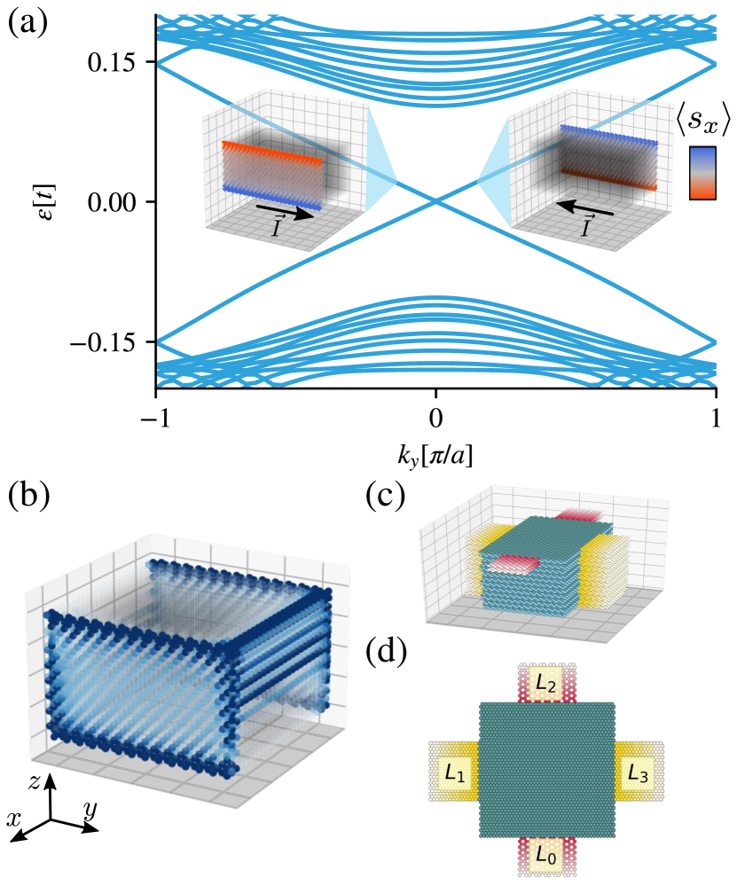
Figure 1: Magnetic TI in the FM phase, $\bm{m}=0.05t\,\hat{z}$. a) Dispersion relation of a slab geometry infinite in the $y$ direction. The left (right) inset depicts the local spin density of states $\langle s_{x}\rangle$ of the edge state at $k_{y}=-0.1\pi/a$ ($k_{y}=0.1\pi/a$). The edge state covers the sidewall of the slab and propagates to the right (left). b) Local density of states of a finite square slab. The edge state circulates around the sample, covers the side surfaces perpendicular to $\hat{x}$, and propagates along the top or bottom hinges of the side surfaces perpendicular to $\hat{y}$. c) Side view of transport setup geometry: metallic leads connect to the whole walls at both ends of the slab (golden color), and ferromagnetic leads connect to the sidewalls only near top hinge (red color). d) Top view and reference numbering of the leads on the transport setup.

We present the main electronic and spin characteristics of the magnetic topological insulator model in Figure 1. The details of the edge modes vary with the geometric design. For a heterostructure infinite along the $y$-direction but finite in both other directions, we obtain the usual linear energy dispersion of topological edge states seen in Fig.1-a). These states cover the whole side surface of the stack (wall-states) with a very large electronic density at the hinges. Interestingly, the projected local spin density of the wall-states is seen to be dominated by the $\langle s_{x}\rangle$ value near the hinges. The hinge spin polarization (HSP) switches sign between opposite surfaces. Furthermore, the HSP changes sign for the back-propagating states, located at the opposite walls (see insets). On a finite slab, Fig. 1-b), the nature of the chiral states becomes richer, with the emergence of hinge states for certain surface cleavage orientations, a property predicted for Möbius fermions Zhang et al. (2013, 2020); Plekhanov et al. (2020). The Möbius fermions phase depends on the ferromagnetic interlayer exchange, and appears in the FM and canted-AFM phase on crystalline canting directions. Conversely, the HSP is robust and appears in all phases, that is: FM, AFM, and canted-AFM, irrespective of the canting angle, as long as there is a $z$-component of the net magnetization. We next explore the possible fingerprints of such anomalous spin features on quantum transport in the QAH regime.

Multi-terminal spin transport simulations. — To analyse the spin transport in the QAH regime, we use the Kwant software package Groth et al. (2014) to build the three-dimensional model, and implement a multi-terminal device configuration, shown in Figs. 1 c), and d). We perform charge transport simulations of a central scattering region connected with metallic and ferromagnetic leads. The interplay between the states available for transport in the leads and in the scattering region has a central role. The leads $L_{1}$ and $L_{3}$ are the metallic leads (golden color). They are fully contacting the left and right sides of the slab (all spin projections). The ferromagnetic leads $L_{0}$ and $L_{2}$ (red color) located on the sides only contact the upper part of the device near the top hinge [AsimilardevicecanbeenvisionedtomeasuretheAxioninsulatorphase]RChen2020. They carry electrons with only one spin polarization: $(s_{x},\downarrow)$. In this way, these contacts couple with the edge state in the region of maximal local spin polarization.

The expected resistance measurements for the QAHE are shown on the inset of Fig. 2. We use the notation $R_{ij,kl}$, for the resistance measured from passing current between terminals $i$ and $j$, and measuring the voltage drop between terminals $k$ and $l$. The two-terminals (2T) resistance $R_{kl,kl}$ is noted $R_{2T,kl}$. The typical values of Hall resistance $R_{xy}=R_{13,20}$ and the longitudinal resistance $R_{xx}=R_{01,23}$ of a QAH insulator Büttiker (1988, 1986) take the quantized values $R_{xy}=\frac{1}{C}h/e^{2}$, where $C$ is the Chern number, and vanishing $R_{xx}$ inside the gap. The two-terminal resistance $R_{2T}=h/e^{2}$ is also quantized for perfect tunneling between the leads and the scattering region Note (2). Such is the case of the matching ferromagnetic lead. The matching or mismatching between the spin current carried by the leads and the spin polarization of the edge states gives rise to a remarkable resistance switch, as seen in Fig. 2. The 2T resistance in the matching case is quantized inside the topological gap, while in the mismatching case the resistance increases by more than one order of magnitude.

To test the robustness of the 2T resistance switching effect, we introduce different types of disorder. First, we consider the impact of structural disorder—vacancies near the sidewalls of the slab. This disorder is detrimental to the formation of well-defined HSP, which only occur for wall-states at crystalline edges. Nevertheless, is relevant for predictions on experiments, since the side walls of material samples have edge disorder. We find that the HSP effect survives to structural disorder, up to $\%5$ vacancies Note (1). Next, we simulate Anderson disorder by adding an onsite energy $d\chi$, where $\chi$ is a random variable with normal distribution on $[-0.5,0.5)$. We find robustness of the HSP up to $d$ much larger than the magnetization strength. In Fig. 2, we use $d=2\lvert\bm{m}\rvert=0.04\,t$, and average the resistance curve over $10$ disorder realizations. We see that spin transport measurements can still distinguish the peculiar spin texture of the edge states.

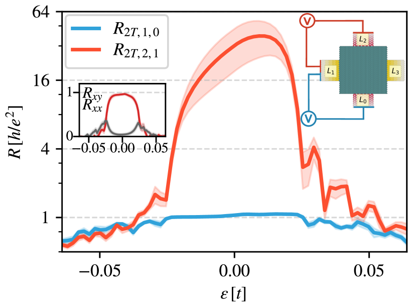
Figure 2: Transport simulations of a FM slab ($\bm{m}=0.02t\,\hat{z}$) between metallic leads and ferromagnetic leads with spin down $(s_{x},\downarrow)$ polarization. The shaded regions depict the standard error of considering $10$ Anderson disorder realizations of strength $d=0.04\,t$. A 4-terminals device allows to measure the distinct resistance profiles. The two-terminal resistance setup between leads $L_{0}$ and $L_{1}$ is depicted on the left inset and the blue curve is the resistance profile. The right inset shows the resistance setup between leads $L_{1}$ and $L_{2}$, with resistance profile in red. In the former case the ferromagnetic lead polarization matches the top HSP, and in the latter case and in the second case the local spin polarization is opposite.

The fact that Anderson disorder and structural disorder show the resistance switch is crucial in establishing the robustness of our results. The limit mismatching case, where the edge state a ferromagnetic lead are completely decoupled from the transport setup, results in voltage probes that have zero transmission probability to any other leads, leaving a floating probe with an arbitrary value of the chemical potential and the voltage Note (3). However, in our case the ferromagnetic leads are not fully disconnected when the spins do not match, rather they are weakly connected. Even though the value of the 2T resistance is sensitive to the details of the weak coupling, seen on the large standard error in Fig. 2, the trend is clear. In a QAH thin-film contacted on its lateral sides with ferromagnetic leads, we can selectively get, either full transmission, or blocking of the edge state transport. Such phenomenon is sensitive to the direction of the magnetization of the ferromagnetic leads, the direction of the current, and the net magnetization of the sample.

Another experimentally relevant analysis is to explore the resistance switch for different directions of the magnetization $\bm{m}$ of the slab in the FM phase. Figure 3 shows two measures of 2T resistance, as in Fig. 2 at the charge neutrality point, for different directions of the Zeeman exchange field $\left(\cos{\theta}\cos{\phi}\hat{x}+\sin{\theta}\cos{\phi}\hat{y}+\sin{\phi}\hat{z}\right)$ (see right inset). At low $\phi$ angles ($\bm{m}$ pointing mostly towards $+\hat{z}$) the configuration $R_{2T,1,2}$ in a) shows large resistance, while $R_{2T,0,1}$ in b) is close to the quantized value $h/e^{2}$. When sweeping the magnetization to the inverse direction (towards $-\hat{z}$) at $\phi~{}180^{\circ}$, the roles of a) and b) reverse, giving a clear signature of the highly spin-polarized hinges and of the spin-dependent matching and mismatching with the ferromagnetic leads. In the middle of both extremes where $\phi=90^{\circ}$, the magnetization lies in the plane of the slab and does not open a gap on the top and bottom surfaces. At intermediate angles, we note that the resistance switch is more robust for $\theta=90^{\circ}$, where $\bm{m}$ tilts towards $\hat{y}$, the transport direction and edge direction that the FM leads contact.

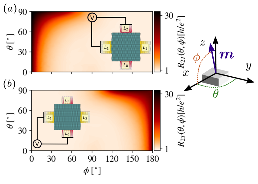
Figure 3: 2T resistance at $e_{F}=0$ of a magnetic TI slab in the FM phase, with magnetization $\lvert\bm{m}\rvert=0.02\,t$ (see right inset). In a) the two-terminal resistance is measured between leads $L_{1}$ and $L_{2}$; in b) the resistance is measured between leads $L_{0}$ and $L_{1}$. The plots in a) and b) are almost identical by reflecting around $\phi=90^{\circ}$, where the magnetization component along the $z$-axis changes sign. The mismatching configurations $\phi=0^{\circ}$ in a), and $\phi=180^{\circ}$ in b) shows the largest resistance, that slowly decreases when rotating the magnetization angle.

The HSP of the edge states is a good proxy to predict the switch in resistances that is measured in the device shown in Fig. 3. We obtain the spin projection of the forward propagating edge states on the top half of an infinite slab in the $\hat{y}$ direction, and finite in the $xz$ plane, see insets of Fig. 4. At momentum $k=-0.02\pi/a$ we select the positive eigenvalue inside the topological gap, similar to the states shown in the insets of Fig. 1-a). Panels a) and b) of Fig. 4 show finite length arrows that indicate the spin density and components in the $(\langle s_{x}\rangle,\langle s_{z}\rangle)$ plane of the forward propagating state, while the color represents the mostly null $\langle s_{y}\rangle$ component. A vanishing arrow length (a point in the plot) indicates that there is no net spin density at that region enclosing that hinge Note (4). When the system is in the topological phase ($\phi\nsim 90^{\circ}$), there is electronic density in one edge or the other, and spin density near the hinge (a finite arrow). Accordingly, we see that panel b) complements perfectly panel a). In both cases the HSP direction changes with the magnetization angle, giving a notch to control the matching or mismatching cases in a transport setup.

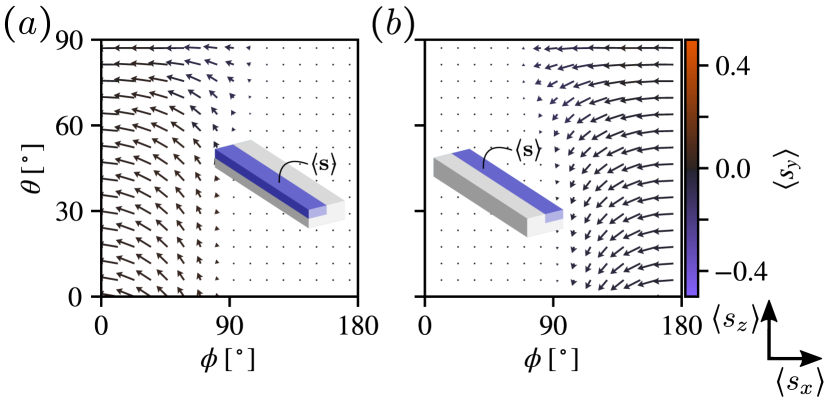
Figure 4: Magnetic TI slab with the same parameters as in Fig. 3. HSP of the edge state at $k_{y}=-0.02\pi/a$ and positive energy (propagating in the $\hat{y}$ direction) for a wide range of magnetization angles $(\theta,\phi)$. The arrows show the components of $\langle{s}\rangle$ projected on the top- left (-right) hinges of an infinite slab along the $y$-axis. The direction of the arrows gives the component in the $(\langle s_{x}\rangle,\langle s_{z}\rangle)$ plane, and the color of the arrows is the component in $\langle s_{y}\rangle$. a) Propagating edge states on the top-left hinge are only present when the magnetization has a positive projection along $z$, thus $\phi\lesssim 90^{\circ}$. b) Propagating edge states on the top-right hinge are only present when the magnetization has a negative projection along $z$, thus $\phi\gtrsim 90^{\circ}$.

Conclusions. — We have demonstrated that the edge states in thin-film ferromagnetic and antiferromagnetic TIs host HSP, spin polarized states at the hinges, which leads to a large resistance switch. The HSP of the edge states is in-plane, but the sign depends on the propagation direction and the magnetization of the sample. For a crystalline edge direction, the local spin polarization reverses across the vertical direction. Thus, the HSP inverts across the vertical direction, and switches sign for the opposite current direction. Carefully engineering ferromagnetic contact leads in a transport setup, allows us to obtain a giant resistance (spin valve effect) upon reversing the current direction or, conversely, tuning the total magnetization of the sample. The $\langle s_{x}\rangle$ component of the spin direction in Fig. 4 a) and b) can be directly translated to the resistance values found in Fig. 3 a) and b). This highlights that the resistance switching mechanism, once established, can be used to gain insight about the magnetization of the sample.

We finally observe that the fact that FM and AFM topological insulators are able to host maximally spin polarized currents along crystalline hinges opens new avenues to implement disruptive proposals using Axion and magnetic TIs to manipulate dislocation, hinge, and edge states Varnava and Vanderbilt (2018), with the additional value of spin polarization features.

Supplemental Material

Appendix S2 Spin texture of the Fu-Kane-Mele model with Zeeman field

The Fu-Kane-Mele Fu and Kane (2007); Fu et al. (2007); Soriano et al. (2012); Pershoguba and Yakovenko (2012) (FKM) model is a versatile model of topological insulators that can reproduce $1$ or $3$ Dirac cones on the surface, depending on the surface termination. If Fig. S1 we show the case of one Dirac cone at each surface of a two-dimensional slab, finite in the $z$-direction. We obtain one Dirac point (per surface) located at the $\Gamma$ point by setting the surface termination to $A(B)$ at the top (bottom) surface, and $t_{4}=t^{\prime}$, $t_{i}=t$ for $i=1,2,3$, with $t^{\prime}>t$. With a small but finite Zeeman field, the Dirac cones at each surface become massive, giving rise to the QAH phase.

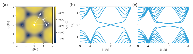
Figure S1: (a) Fermi level resolved in $\bm{k}$ space of a FKM slab with $12$ layers. The Dirac point appears at the $\Gamma$ point. The dotted gray line delimits the Brillouin zone, and high-symmetry points are denoted with white dots. The k-path is traced with a white line connecting the high-symmetry k-points. The band-structure following the k-path is depicted in (b) for zero Zeeman field, and in (c) for finite Zeeman field ($\lvert\bm{m}\rvert=0.1\,t$).

The spin texture in Fig. S2-(a) of the FKM model compares qualitatively well with that of $\text{Bi}_{2}\text{Te}_{3}$ Liu et al. (2010). The model reproduces the time-reversal symmetry $\mathcal{T}$, and three-fold rotation symmetry $\mathcal{C}_{3}$, while the bulk gap can be tuned by $\Delta t=t^{\prime}-t$ and the spin-orbit coupling strength $\lambda_{SO}$.

In Fig. S2 (b) we show the spin texture in the Quantum Anomalous Hall phase. A crystalline termination along the $y$ direction (and $3$-fold rotation symmetric directions) hosts bulk states with zero net spin polarization in the $xy$-plane. The edge states inherit the same pattern, giving a zero net spin polarization in the $xy$-plane. This is also a consequence of one edge mode hosting two hinge spin polarizations near the top and bottom surfaces, that cancel each other out exactly.

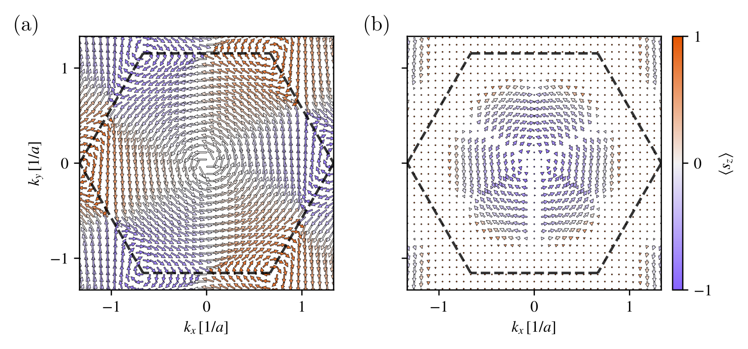
Figure S2: Spin texture of the FKM model. (a) without Zeeman field, and (b) with Zeeman field $\lvert\bm{m}\rvert=0.05\,t$.

Appendix S3 Spatial profile of the edge-states

The edge-states carrying hinge spin polarization (HSP) are wall-states (as opposed to hinge-states). They cover the whole side of the slab, and host finite electronic density throughout. This means that the top and bottom HSP form part of the same state, and injecting current on either, will propagate the electronic density to the other hinge. As a consequence of the non-conservation of the spin in a system with strong spin-orbit coupling (SOC), even if injecting perfectly spin-polarized current, when propagating through the slab, the spin-polarization of current will take the values dictated by the two HSPs.

To demonstrate this, we show in Fig. S3 the spatial profile of one edge-state with the two HSPs. The markedly high (spin-polarized) electronic density at the hinges is a result of the half-quantized topological charge. A signature of the surfaces hosting Dirac states at zero Zeeman field, and these electronic modes being pushed to the hinge at small but finite Zeeman field.

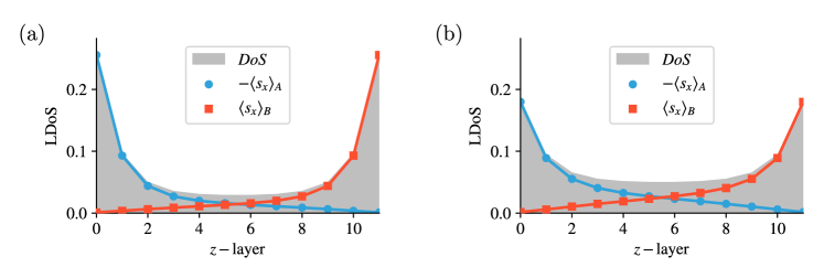
Figure S3: Spatial profile of the local density of states (LDoS) and spin projection per layer of one edge state located at $k=0.05\,a^{-1}$ and positive energy. The single edge state has distinct sublattice and spin profiles. The spin projection $\langle s_{x}\rangle$ of sublattice $A$ is shown in blue circles, and the one of sublattice $B$ in red squares. In (a) the magnetization is $\bm{m}=0.05\,t\hat{z}$, while in (b) is $\bm{m}=0.1\,t\hat{z}$. Note the HSP is sublattice polarized, and that we reversed the sign of $\langle s_{x}\rangle_{A}$.

Appendix S4 Structural disorder simulations

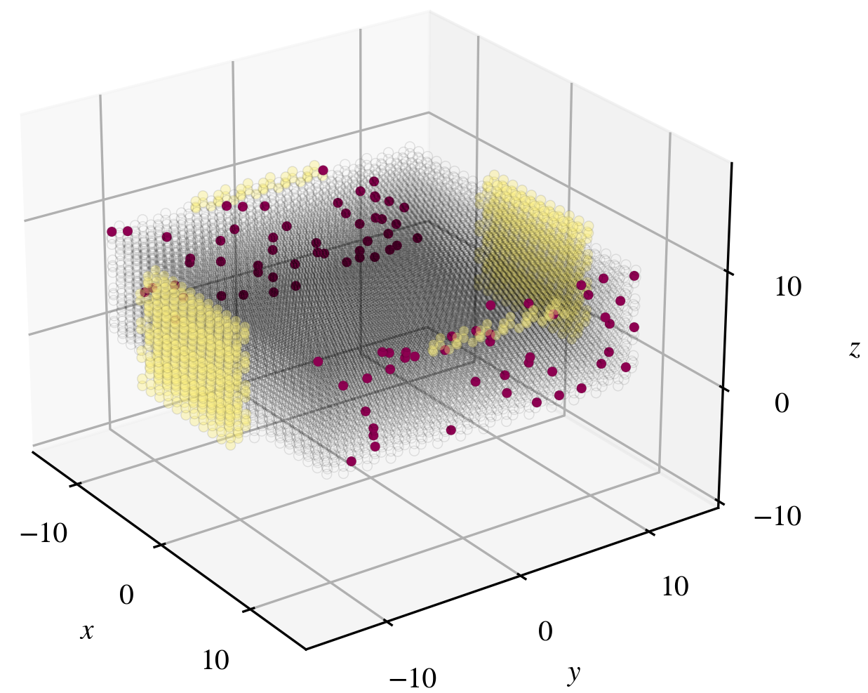
Figure S4: One realization of structural disorder at the edges of a slab. The probability of removal is $p=0.05$ for all sites within $3$ lattice constants from the edge parallel to the $y$ axis. The sites in purple are eliminated from the transport setup. One unitcell of the leads connected to the slab are depicted in golden color.

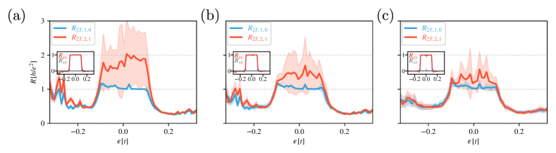
Figure S5: Resistance measurements simulations for slabs with structural disorder. The blue lines depict the matching case $R_{2T,1,0}$, while the red lines the mismatching case $R_{2T,2,1}$. The inset shows the typical non-local resistance measurements $R_{xx}$ and $R_{xy}$. The shaded region around the lines depict the standard deviation taken from $16$ disorder realizations. The panels (a), (b) and (c) correspond to $p=0.01$, $p=0.02$, and $p=0.05$, respectively.

To test the robustness of the HSP we have performed simulations with structural disorder. We remove atomic sites randomly near the edges of the slab, in the closest three unit-cells near the walls, with a probability $p$, as shown in Fig. S4. Note that we remove sites from a within $3$ lattice constants from the edge. Since we remove each site with the same probability, for example $\%5$, then the probability at any point on the side wall that at least one of the sites is removed is much larger, around $\%14$. We find that the spin-valve effect is distinguishable with small structural disorder (Fig. S5), and survives up to a structural disorder of $p=5\%$. While the two-terminal resistance in the matching case remains quantized to the Hall resistance value, the mismatching case shows a clear deviation from quantization that is dependent on the details of the disorder realization. In Fig. S5 we show the averaged results for $16$ disorder realization, with shaded regions around the curves to depict the standard deviation.

Other types of disorder, such as magnetic disorder, or a combination with energetic disorder to mimic the effect of magnetic dopants, are not simulated further in this Supplemental Material nor the main Letter. However, we anticipate them to be detrimental to the hinge spin polarization (HSP). Since we have demonstrated the robustness of the HSP against energetic (Anderson) disorder and structural disorder, we expect that there will also be a range of magnetic doping in which the resistance signatures of the HSP are clearly discernible.

References

- Fu and Kane (2007) L. Fu and C. L. Kane, Topological insulators with inversion symmetry, Physical Review B 76, 045302 (2007).
- Fu et al. (2007) L. Fu, C. L. Kane, and E. J. Mele, Topological Insulators in Three Dimensions, Physical Review Letters 98, 106803 (2007).
- Soriano et al. (2012) D. Soriano, F. Ortmann, and S. Roche, Three-Dimensional Models of Topological Insulators: Engineering of Dirac Cones and Robustness of the Spin Texture, Physical Review Letters 109, 266805 (2012).
- Pershoguba and Yakovenko (2012) S. S. Pershoguba and V. M. Yakovenko, Shockley model description of surface states in topological insulators, Physical Review B 86, 075304 (2012).
- Liu et al. (2010) C.-X. Liu, X.-L. Qi, H. Zhang, X. Dai, Z. Fang, and S.-C. Zhang, Model Hamiltonian for topological insulators, Physical Review B 82, 045122 (2010).