A new analytical approximation of luminosity distance by optimal HPM-Padé technique

Abstract

By the use of homotopy perturbation method-Padé (HPM-Padé) technique, a new analytical approximation of luminosity distance in the flat universe is proposed, which has the advantage of significant improvement for accuracy in approximating luminosity distance over cosmological redshift range within $0\leq z\leq 2.5$. Then we confront the analytical expression of luminosity distance that is obtained by our new approach with the observational data, for the purpose of checking whether it works well. In order to probe the robustness of the proposed method, we also confront it to supernova type Ia and recent data on the Hubble expansion rate $H(z)$. Markov Chain Monte Carlo (MCMC) code emcee is used in the data fitting. The result indicates that it works fairly well.

1 Introduction

Recent astronomical observations clearly indicate that the universe is currently expanding with an increasing speed, and is spatially flat and vacuum dominated[1,2]. In order to explain this mysterious phenomenon, many cosmological models[3] have been proposed. Since the relation between cosmological distances and redshift depends on the parameters of underlying cosmological models, the accurate and efficient analytical computation of these cosmological distances becomes an important issue for the comparison of different cosmological models with observation data in modern precision cosmology.

As is well known to all, in the general lambda cold dark matter ($\Lambda$CDM), luminosity distance which is the most important distance from an observational point of view, can only be expressed in the term of integrals over the cosmological redshift, and computation pressure of the integral of luminosity distance is usual very large. Therefore, for the purpose of avoiding numerical quadrature , several analytical approaches[4,5,6,7,8,9]to approximate luminosity distance in flat universe have been proposed for decades. Among these methods, one of the most widely used approaches is to apply Taylor expansion to approximate luminosity distance[10,11]. Obviously, Taylor polynomial expanding at $z=0$ may have divergence problem caused by cosmological observations that exceed the limits of it. In fact, the supernova data that we obtain now is at least back to $z\approx 2.35$ data available[10,11]. Thus several works suggested [11,13,14] that Padé rational polynomial has the ability to approximate luminosity distance, due to its good convergence property in a relatively larger redshift range.

In addition, by solving the differential equation of luminosity distance, Shchig- olev and Yu obtained two formulae for approximating luminosity distance with smaller error over a relatively small redshift interval based on homotopy perturbation method(HPM)[9](hereafter Shch17) and optimal homotopy perturbation method (OHPM)[15], respectively. The HPM was first put forward by He[16] to solve nonlinear differential equations, which yields a very accurate solution via one or two iterations. After that various modifications of HPM[17,18,19]were given by various investigators, such as the OHPM coupled with the least squares method[19,20], optimal homotopy asymptotic method[21], and so forth. In a word, we can obtain more accurate approximations for luminosity distance over a relatively small redshift interval,based on the use of HPM technique(or modifications of HPM ). Thus, to reach a compromise between accuracy and redshift convergence interval, the combination of padé approximant and HPM are therefore adequate candidates to carry out this goal. In fact, homotopy perturbation method-Padé technique(HPM-Padé) has been recognized as a good one to apply the series solution to improve the accuracy and enlarge the convergence interval[22,23] in the study of nonlinear differential equations.

Therefore, in this paper, we will apply HPM-Padé to obtain a more accurate approximate analytical expression for luminosity distance in a relatively larger redshift range, based on solving the differential equation of luminosity distance in a flat universe. The rest of this paper is as follows. In Section 2, we briefly review the differential equation of luminosity distance $d_{L}$ in a spatially flat universe. The HPM-Padé rational approximation of luminosity distance $d_{L}$ is given in Section 3. In Section 4, comparison of our rational approximation polynomial for computing luminosity distance is made with the results obtained other existing methods. Then we confront the analytical approximate expression of luminosity distance that was obtained by HPM-Padé technique with the observational data, for the purpose of checking whether it works well. Note that Markov Chain Monte Carlo (MCMC) code emcee[24] is used in the data fitting. Finally, some brief conclusions are given in Section 5.

2 Differential equation of luminosity distance in a flat universe

The general expression of theoretical modulus in a flat universe is defined as follows[1,2]

$$\mu{(z)}=5\log_{10}{(\frac{d_{L}}{Mpc})}+25$$ (1)

where $d_{L}$ is the luminosity distance. In order to verify theoretical calculation, we difine the luminosity distance $d_{L}$ of SNe Ia in a flat $\Lambda$CDM universe as follows[25]

$$d_{L}(z)=\frac{c(1+z)}{H_{0}}\int_{0}^{z}\frac{dt}{\sqrt{\Omega_{m}(1+t)^{3}+\Omega_{\Lambda}}},$$ (2)

where $\Omega_{m}$ and $\Omega_{\Lambda}$ are the energy densities corresponding to matter and cosmological constant, respectively: $\Omega_{m}+\Omega_{\Lambda}=1$, $c$ is the speed of light, $z$ is cosmology redshift, and $H_{0}$ is the Hubble constant.

As mentioned in Shch17, we define $W(z)$ as follows

$$W(z)=\Omega_{m}(1+z)^{3}+\Omega_{\Lambda},obviously,W(z)|_{z=0}=1.$$ (3)

Then Eq.(2) can be rewritten as:

$$\frac{d_{L}(z)H_{0}}{c(1+z)}=\int_{0}^{z}\frac{dt}{\sqrt{W(t)}}.$$ (4)

For simplicity,we introduce:

$$1+z=x,u(x)=\frac{d_{L}(z)H_{0}}{cx},$$ (5)

Then, we get

$$u(x)=\int_{0}^{x-1}\frac{dt}{\sqrt{W(t)}}.$$ (6)

By differentiating the Eq.(6), we can obtain

$$u^{{}^{\prime}}(x)=\frac{1}{\sqrt{W(x-1)}}.$$ (7)

Combining the Eq.(2),(3),(4),(5) and (6), we have

$$u^{{}^{\prime}}(x){|_{x=1}}=1,u(x)|_{x=1}=0.$$ (8)

According to Eq.(7) and (8),we can derive the Cauchy problem as follows:

$$u^{{}^{\prime\prime}}+\frac{1}{2}W^{{}^{\prime}}(x-1){u^{{}^{\prime}}}^{3}=0;u^{{}^{\prime}}(x){|_{x=1}}=1,u(x)|_{x=1}=0.$$ (9)

where the prime is the derivative with respect to $x$, and $W(x-1)|_{x=1}=1$.

3 HPM-Padé rational approximation of luminosity distance ${d_{L}}$

3.1 Solution of Homotopy perturbation method

For the homotopy perturbation technique has already become standard and concise, its basic idea can be referred to[16,17]. In order to solve Eq.(9) by homotopy perturbation technique, we build the homotopy as follows:

$${u^{\prime\prime}}+c_{1}+p\left[\frac{1}{2}{W^{\prime}}(x-1){u^{\prime}}^{3}-c_{1}\right]=0,$$ (10)

Let us assume that the solution of Eq.(10) in the form of a series in $p$ :

$$u=u_{0}+pu_{1}+p^{2}u_{2}+p^{3}u_{3}+\dots,$$ (11)

Substituting Eq.(11) into Eq.(10), and collecting coefficients with the same power of $p$, we get a set of differential equations :

$$p^{0}: {u_{0}}^{{}^{\prime\prime}}+c_{1}=0,$$ (12)

$$p^{1}: {u_{1}}^{\prime\prime}+\frac{1}{2}W^{\prime}(x-1){{u_{0}}^{\prime}}^{3}-c_{1}=0,$$ (13)

$$\dots\dots\dots\dots$$

From Eq.(9), we can obtain the initial conditions as follows:

$${u_{0}}{|_{x=1}}=0,~{}{u_{0}}^{\prime}{|_{x=1}}=1;$$

$${u_{i}}{|_{x=1}}=0,~{}{u_{i}}^{\prime}{|_{x=1}=0};$$ (14)

where $i\geq 1$.

We now can solve the above differential equations with the initial conditions Eq.(14). Thus, we successively get

$$u_{0}=(x-1)-\frac{c_{1}}{2}(x-1)^{2},$$ (15)

$$\begin{split}u_{1}=&\frac{1}{2}(x-1)+\frac{c_{1}}{2}(x-1)^{2}-\frac{1}{2}\int_{1}^{x}W(t-1)\\ &\times{\left[1-c_{1}(t-1)\right]}^{2}\{1-c_{1}\left[4(t-1)-3(x-1)\right]\}dt,\end{split}$$ (16)

and so on. By setting $p=1$ in Eq.(11),we get the approximate analytical expression of luminosity distance

$$\widetilde{d}_{L}(z)=\frac{c(1+z)}{H_{0}}\{z+\alpha_{1}z^{2}+\alpha_{3}z^{3}+\dots++\alpha_{k}z^{k}+\dots\}$$ (17)

where $c$ is the speed of light, $H_{0}$ is the Hubble constant, $z$ is redshift, and $\alpha_{k}(k\geq 1)$ are functions of the unknown constant $c_{1}$.

3.2 Padé approximate technique to the series solution of differential equation for luminosity distance ${d_{L}}$

Padé approximate technique is the best approximation of a function $f(z)$ by a rational polynomial of a given order($m$,$n$)[26]

$$P_{mn}(z)=\frac{a_{0}+a_{1}z+\dots+a_{m}z^{m}}{1+b_{1}z+\dots+b_{n}z^{n}}$$ (18)

In order to determine coefficients of Padé approximation of order($m$,$n$), let us assume $f(z)$ can be expanded in the form of a power series in $z$ as follows:

$$f(z)=\sum\limits_{k=0}^{m+n+1}{d_{k}z^{k}}$$ (19)

Generally, $f(z)$ is expanded in Taylor series about at the point $z=a$. In this study, as mentioned above in Section 2, the approximate analytical expression of luminosity distance $\widetilde{d}_{L}$ obviously has similar form of a power series in $z$. For convenience, let us rewrite the approximate analytical expression of luminosity distance(Eq.(17)) $\widetilde{d}_{L}$ as

$$\widetilde{d}_{L}(z)=\sum\limits_{k=0}^{m+n+1}{d_{k}z^{k}}$$ (20)

So,we obtain

$$\widetilde{d}_{L}(z)-\frac{a_{0}+a_{1}z+\dots+a_{m}z^{m}}{1+b_{1}z+\dots+b_{n}z^{n}}=O(Z^{n+m+1})$$ (21)

Then the Eq.(21) can be written out as

$$\begin{split}&d_{m+1}+d_{m}b_{1}+\dots+d_{m-n+1}b_{n}=0\\ &d_{m+2}+d_{m+1}b_{1}+\dots+d_{m-n+2}b_{n}=0\\ &\vdots\\ &d_{m+n}+d_{m+n}b_{1}+\dots+d_{m}b_{n}=0,\end{split}$$ (22)

$$\begin{split}&a_{0}=d_{0}\\ &a_{1}=d_{1}+d_{0}b_{1}\\ &a_{2}=d_{2}+d_{1}b_{1}+d_{0}b_{2}\\ &\vdots\\ &a_{m}=d_{m}+d_{m-1}b_{1}+\dots+d_{0}b_{m},\end{split}$$ (23)

From Eq.(22),we can get the $b_{i}(1\leq i\leq n)$. By the known values of $b_{1},b_{2},\dots,b_{n}$, we can obtain the values of $a_{0},a_{1},\dots,a_{m}$ from the Eq.(23).Then we obtain the approximate analytical expression of luminosity distance as follows:

$$\widetilde{d}_{L}(z)=\frac{c}{H_{0}}\frac{a_{0}+a_{1}z+\dots+a_{m}z^{m}}{1+b_{1}z+\dots+b_{n}z^{n}}$$ (24)

where $c$ is the speed of light, $H_{0}$ is the Hubble constant, $z$ is redshift, and $b_{i}(1\leq i\leq n)$ and $a_{k}(0\leq k\leq m)$ are functions of the unknown constant $c_{1}$.

The relative error of the approximation for the luminosity distance is given by[5]

$$\bigtriangleup E=\left|\frac{\widetilde{d}_{L}-d_{L}^{num}}{d_{L}^{num}}\right|$$ (25)

where $d_{L}^{num}$ and $\widetilde{d}_{L}$ stand for the values of luminosity distance calculated from the numerical method and our HPM-Padé approximate expression, respectively.

Many methods, such as the least square method[19,20] and the collocation method [27], can be used to optimally determine the unknown constant $c_{1}$. As similar in our previous work[15], by minimizing the relative error, we optimally determine unknown constant $c_{1}$, which yields the following algebraic equation

$$\frac{\partial\bigtriangleup E}{\partial C_{1}}=0$$ (26)

Significantly, it is very important to choose the orders ($m,n$) of the rational polynomial for luminosity distance, which may lead to divergence problems and bias its corresponding numerical results. From one hand, the uncertainties of the free coefficients ($b_{i}(1\leq i\leq n)$and $a_{k}(0\leq k\leq m)$) increases when the orders are too high and the number of coefficients is too many; on the other hand, the accuracy of the rational polynomial in approximating for luminosity distance will be small when the number of coefficients is too little. Given this fact, in order to make sure the rational approximations to be convergent, it is essential to consider a small number of free coefficients. Zhou choosed a moderate order($2,2$) in the work of Padé parameterization of the luminosity distance [13]. S. Capozziello pointed out that the order($2,1$) of Padé approximation for the luminosity distance (Hereafter P(2,1)) is better way to explain high-low cosmological redshift data[11].To our knowledge, the best way to this issue on orders choice of rational polynomial is to analysize the above mentioned ones with different orders.

4 Performance of the HPM-Padé rational approximation

In this section, the performance of HPM-Padé rational approximation in Sect.3 is assessed, which includes two steps. Firstly, comparison of our proposed approach for computing $\Lambda$CDM model luminosity distance is made with the results obtained by other methods. Then we confront the analytical expression of luminosity distance that was obtained by the HPM-Padé technique with the observational data, for the purpose of checking whether it works well.

4.1 HPM-Padé approximation versus other methods for the $\Lambda CDM$ model

To help visualize this goal, we will give a qualitative representation of the improvements for accuracy in approximating luminosity distance, which is obtained by performing HPM-Padé technique.

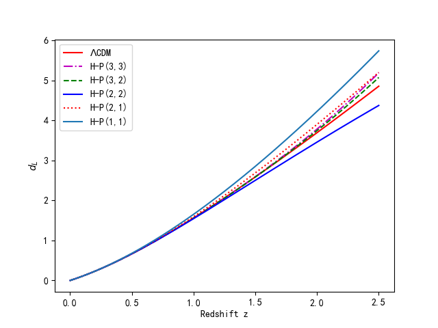
Figure 1: The curves of luminosity distance $d_{L}$ for the $\Lambda$CDM model when $\Omega_{m}=0.28$ and the comparison with the numerical behavior of HPM-Padé approximation with different orders over the range of redshift $0<z\leq 2.5$.

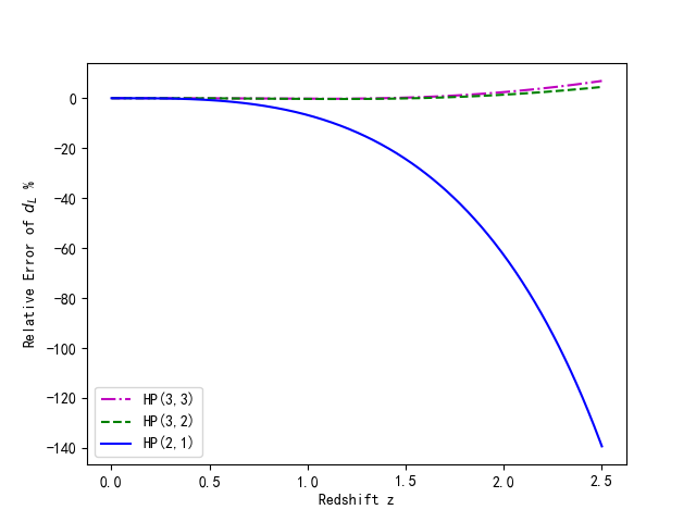
Figure 2: When $\Omega_{m}=0.28$, relative error percentages of rational approximations for $d_{L}$($\bigtriangleup E$) in the $\Lambda$CDM model with third order H-P(2,1), fifth order H-P(3,2) and sixth order H-P(3,3), when $\Omega_{m}=0.28$.

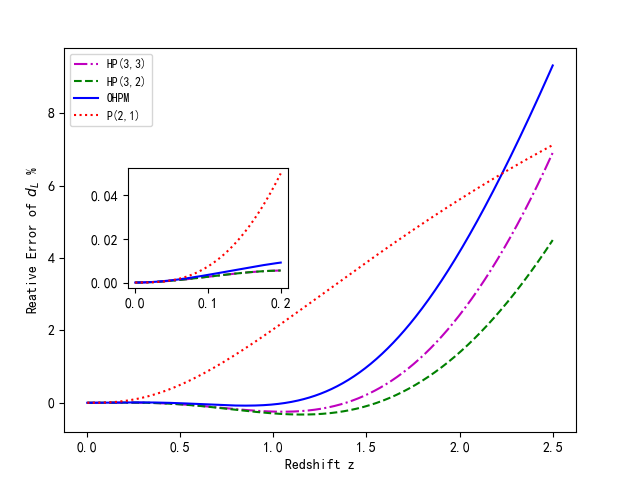
Figure 3: For the fixed $\Omega_{m}=0.28$, relative error percentages of approximate for $d_{L}$($\bigtriangleup E$) in the $\Lambda$CDM model obtained by different approximation techniques.The relative error percentages of $d_{L}$ over range $0\leq z\leq 0.2$ is amplified,which is shown in the inset.

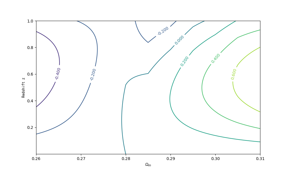
Figure 4: The contour for the distribution of relative error percentages of H-P(3,2) for $d_{L}$($\bigtriangleup E$) in the $\Lambda$CDM model by use of HPM-Padé approximate to corresponding to $\Omega_{m}$ within $0.26\leq\Omega_{m}\leq 0.31$ and over redshift interval $0\leq z\leq 1$. The global error is dominated by the“peaks”and“pits” in the region.

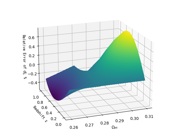
Figure 5: The global relative error surface of approximation H-P(3,2) for $d_{L}$($\bigtriangleup E$) in the $\Lambda$CDM model corresponding to $\Omega_{m}$ over the span $0.26\leq\Omega_{m}\leq 0.31$. When the variation of $\Omega_{m}$ from 0.26 to 0.31, the relative error increases. When the variation of cosmological redshift $z$ from 0 to 1,the relative error first increases and then decreases within the range $0.28\leq\Omega_{m}\leq 0.31$, and the relative error first decreases and then increases within the range $0.26\leq\Omega_{m}\textless 0.28$.

For the elucidative purposes, in Fig.1, we plot analytical curves of luminosity distance $d_{L}$ for the $\Lambda$CDM model and the comparison with the numerical behavior of HPM-Padé approximation with different orders over the range of redshift $0\leq z\leq 2.5$. From the Fig.1, rational HPM-Padé polynomial of third order H-P(2,1), fifth order H-P(3,2) and sixth order H-P(3,3) have been selected according to their good behaviors over the range of redshift $0\leq z\leq 2.5$. Fig. 2 shows the relative error percentages of $d_{L}$($\bigtriangleup E$)for third order H-P(2,1), fifth order H-P(3,2) and sixth order H-P(3,3), which indicates that fifth order H-P(3,2) and sixth order H-P(3,3) behave significantly well in approximating $\Lambda$CDM model luminosity distance.

In Fig. 3, the comparison of fifth order H-P(3,2) and sixth order H-P(3,3) for computing $\Lambda$CDM model luminosity distance is made with the results obtained by some existing methods such as OHPM and P(2,1).The HPM-Padé approximation is superior to other methods, because the relative error percentage $\bigtriangleup E\approx 4\%$ is reached at $z=2.437$ for HPM-Padé approximation with order(3,2), at $z=1.959$ for optimal homotopy perturbation method, and at $z=1.540$ for Padé approximation with order(2,1); the relative error percentages $\bigtriangleup E$ at $z=0.2$ are 0.0053% for HPM-Padé approximation with order(3,2)(or order(3,3)), 0.0099% for optimal homotopy perturbation method, and 0.0498% for Padé approximation with order(2,1), respectively. Fig.4 shows that the relative error percentages range of H-P(3,2) for $d_{L}$ in $\Lambda$CDM model is from -0.4% to 0.6% for any cosmological redshift within $0\leq z\leq 1$ over the $\Omega_{m}$ span $0.26\leq\Omega_{m}\leq 0.31$. Seen from Fig.5, we can get that the relative error increases when the variation of $\Omega_{m}$ from 0.26 to 0.31; the relative error first increases and then decreases within the range $0.28\leq\Omega_{m}\leq 0.31$, and the relative error first decreases and then increases within the range $0.26\leq\Omega_{m}\textless 0.28$.

Obviously, the above figures indicate that, provided we are given data over the relatively larger cosmological redshift interval, HPM-Padé technique would be better way to fit the observed luminosity distances by means of a rational polynomial, for the purpose of getting a more accurate approximate function. Given this fact,we can obtain a better bounds on the parameters of rational HPM-Padé approximation polynomial, which is exactly what we expect.

4.2 Experimental analysis of Type Ia supernova and OHD data with HPM-Padé approximation

Based on the HPM-Padé approximation polynomial of luminosity distance, we can obtain the distance modulus approximation as a function of $H_{0}$, $z$ and $c_{1}$:

$$\widetilde{\mu}{(z)}=5\log_{10}{(\frac{\widetilde{d}_{L}(z)}{Mpc})}+25$$ (27)

Then we confront it with SNIa data to constrain the approximate analytical expression of luminosity distance(Eq.(24)), by use of relation between SNIa data and luminosity distance. Here, we consider the “Pantheon Sample” consisting of 1048 data points within the redshift range $0.01\leq z\leq 2.3$[12] in terms of the distance modulus $\mu_{obs}{(z_{i})}$. By [13], the $\chi^{2}$ from “Pantheon Sample” 1048 SNIa data can be defined as

$$\chi^{2}_{SN}=\sum\limits_{i=1}^{N}\frac{(\mu_{obs}{(z_{i})}-\widetilde{\mu}{(z_{i})})^{2}}{\delta^{2}(z_{i})}$$ (28)

where $N=1048$, and the $\delta(z_{i})$ is corresponding error of observed distance modulus $\mu_{obs}{(z_{i})}$ at $z_{i}$. Correspondingly, a reduced merit function $\chi^{2}_{red}$ becomes:

$$\chi^{2}_{red}=\frac{\chi^{2}_{SN}}{NF}$$ (29)

where the number of degrees of freedom $NF$ is equal to $N-k$, $N$ is the number of SNIa data, and $k$ is the number of parameters of $\widetilde{\mu}{(z)}$. The Akaike information criterion (AIC) [28] is defined by

$$AIC=2k-2\ln(L_{max})$$ (30)

where $L_{max}$ is the maximum likelihood function.

In order to get the best fits, Markov Chain Monte Carlo (MCMC) code emcee[24] was applied on SNIa likelihood. Table 1 reports the numerical results for two parameters of HPM-Padé approximations of luminosity distance. From Table 1, we can see that the constrains on two parameters of rational HPM-Padé approximation polynomial are significantly tightened. Fig.6 shows the best fit for distance modulus(HPM-Padé approximation of order(3,2)).By confronting the HPM-Padé approximation of luminosity distance Eq.(24) with the cosmological observational data, we clearly see that it works fairly well.

As mentioned in[29,30], to probe the robustness of the proposed method, we also confront it to the combination of SNIa data and recent data on the Hubble expansion rate $H(z)$,which includes 31 $H(z)$ measurements that are determined by using the cosmic chronometric technique(see Table 1 in [31]). In fact, we can insert Eq.(24) into

$$H(z)=\left[{\frac{d}{dz}\left(\frac{d_{L}(z)}{1+z}\right)}\right]^{-1}$$ (31)

Table 2 reports the numerical results for two parameters of HPM-Padé approximations with order(3,2)and order(3,3). From Table 2, we can see that the best-fitting values are obtained by HPM-Padé approximation of order(3,3). The marginal distribution function in 1D parameter space, and 1$\delta$, and 2$\delta$ contour in the 2D parameter spaces for the best fitting from SNIa data, combination of SNIa data and OHD data are shown in Fig.7. According to Fig.7, we can get that the constrains on two parameters of rational HPM-Padé approximation polynomial from SNIa data are in good agreement with ones from combination of SNIa data and OHD data. From Table 1 and Table 2, by adding OHD data, the constrains on two parameters are more tightened.

Table 1: MCMC results at the 68.3% (95.4%) C.L for HPM-Padé approximations of luminosity distance from SNIa data. The corresponding AIC and $\chi^{2}_{red}$ are also shown.

. Model $H_{0}$ $c_{1}$ AIC $\chi^{2}_{red}$ HP(3,2) $72.044_{-0.076(-0.149)}^{+0.075(+0.154)}$ $0.4171_{-0.019(-0.038)}^{+0.021(+0.041)}$ 1036.494 0.9890 HP(3,3) $72.039_{-0.074(-0.143)}^{+0.076(+0.151)}$ $0.415_{-0.017(-0.034)}^{+0.019(+0.37)}$ 1036.60 0.9891

Table 2: MCMC results at the 68.3% (95.4%) C.L for HPM-Padé approximations with order(3,2)and order(3,3) from combination of SNIa adta and OHD data. The corresponding AIC and $\chi^{2}_{red}$ are also shown.

. Model $H_{0}$ $c_{1}$ AIC $\chi^{2}_{red}$ HP(3,2) $72.060_{-0.071(-0.141)}^{+0.073(+0.144)}$ $0.431_{-0.015(-0.027)}^{+0.015(+0.030)}$ 1455.07261 0.97742 HP(3,3) $72.050_{-0.071(-0.141)}^{+0.072(+0.142)}$ $0.424_{-0.009(-0.018)}^{+0.0102(+0.021)}$ 1455.07260 0.97727

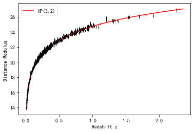
Figure 6: Hubble diagram for Pantheon Sample. The best fit for distance modulus approximation as represented by Eq.(27) with order (3,2) is represented the red solid line.

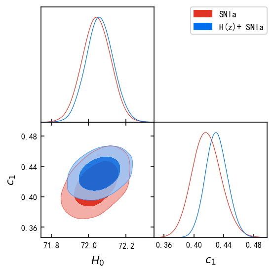
Figure 7: The contour for 1$\delta$, and 2$\delta$ in the 2D parameter spaces, and the marginal distribution function in 1D parameter space. The deep shaded region and light shaded region for each contour stand for 68 percnet confidence level and 95 percent confidence level,respectively.

5 Conclusion and discussion

In this paper, based on use of homotopy perturbation method-Padé (HPM-Padé) technique, a new analytical approximation of luminosity distance in the flat universe is proposed. The numerical results clearly indicate that HPM-Padé technique has obvious advantages in improving accuracy of approximating luminosity distance over relative larger cosmological redshift range interval. It is worthy noting that the choice of the orders ($m,n$) for luminosity distance rational polynomial is very important, which may yield divergence problems and bias its true numerical results. For the elucidative purposes, we make the comparison of rational approximations with different orders for computing $\Lambda$CDM model luminosity distance in Figure 1. Figure 3 indicates that the HPM-Padé approximation is superior to other methods. As an example mentioned above in section 4, the relative error percentage $\bigtriangleup E\approx 4\%$ is reached at $z=2.437$ for HPM-Padé approximation, at $z=1.959$ for optimal homotopy perturbation method, and at $z=1.540$ for Padé approximation, respectively. It means that we can get a larger cosmological redshift range of convergence by HPM-Padé approximation.

According to [29] and [30], to probe the robustness of the proposed method, we confront it to SNIa data, combination of SNIa data and OHD data, respectively. The results indicate the rational HPM-Padé approximation polynomial is robust. Furthermore, the proposed analytical approximation of luminosity distance in the flat $\Lambda$CDM, has the advantage of significant improvement for accuracy in approximating luminosity distance over cosmological redshift range within $0\leq z\leq 2.5$. In other words, the proposed analytical approximation of luminosity distance in the flat $\Lambda$CDM can be trusted up to $z\sim 2.5$, which can avoid a breakdown in the validity of the approximation for luminosity distance over cosmological redshift range within $0\leq z\leq 2.5$ that may be misinterpreted as a (phantom) deviation from $\Lambda$CDM. Due to its model-dependent, rational HPM-Padé approximation polynomial of luminosity distance for $\Lambda$CDM model can not be used to model different dark energy behaviors for different range.[32]. To our knowledge, for methodological reasons, we cannot apply HPM-Padé technique to other cosmological models. Take the $\omega$CDM model as example, we will obtain a series of fractional powers of redshift $z$ during the process of solving differential equation of luminosity distance. As a result, the rational analytic expression of luminosity distance cannot be obtained by using Eq.(21), which causes this technique to be invalid. To conclude, we have put forward and investigated here HPM-Padé technique in approximating luminosity distance. Moreover, HPM-Padé technique can be used in other fields of precision cosmology, due to its good properties.

References

- [1] A. G. Riess, et al., Observational Evidence from Supernovae for an Accelerating Universe and a Cosmological Constant, The Astronomical Journal 116 (3) (1998) 1009–1038.
- [2] S. Perlmutter, G. Aldering, G. Goldhaber, et al., Measurements of Omega and Lambda from 42 High-Redshift Supernovae, The Astrophysical Journal 517 (12) (1999) 565–586.
- [3] M. Li, X.-D. Li, S. Wang, Y. Wang, Dark Energy, Communications in Theoretical Physics 56 (3) (2011) 525–604.
- [4] U.-L. Pen, Analytical Fit to the Luminosity Distance for Flat Cosmologies with a Cosmological Constant, Astron.Astrophys.Suppl.Ser. 120 (1) (1999) 49.
- [5] T. Wickramasinghe, T. N. Ukwatta, An analytical approach for the determination of the luminosity distance in a flat universe with dark energy, Mon. Not. R.Astron.Soc. 406 (1) (2010) 548.
- [6] D.-Z. Liu, C. Ma, T.-J. Zhang, Z. Yang, Numerical strategies of computing the luminosity distance, Mon.Not.R.Astron.Soc. 412 (1) (2011) 2685.
- [7] M. Adachi, M. Kasai, An Analytical Approximation of the Luminosity Distance in Flat Cosmologies with a Cosmological Constant, Prog. Theor. Phys. 127 (1) (2012) 145–152.
- [8] M. Baes, P. Camps, D. Van De Putte, Analytical expressions and numerical evaluation of the luminosity distance in a flat cosmology, Mon. Not. R. Astron. Soc. 468 (1) (2017) 927.
- [9] V. K. Shchigolev, Calculating luminosity distance versus redshift in FLRW cosmology via homotopy perturbation method, Gravitation and Cosmology 23 (2) (2017) 142–148.
- [10] C. Clarkson, C. Zunckel, Direct Reconstruction of Dark Energy, Physical Review Letters 104 (21) (2010) 211301.
- [11] S. Capozziello, R. D’Agostino, O. Luongo, High-redshift cosmography: auxiliary variables versus Padé polynomials, Monthly Notices of the Royal Astronomical Society 494 (2) (2020) 2576–2590.
- [12] D. M. Scolnic, et al., The Complete Light-curve Sample of Spectroscopically Confirmed SNe Ia from Pan-STARRS1 and Cosmological Constraints from the Combined Pantheon Sample, The Astrophysical Journal 859 (2) (2018) 101.
- [13] Y.-N. Zhou, D.-Z. Liu, X.-B. Zou, H. Wei, New generalizations of cosmography inspired by the Padé approximant, European Physical Journal C 76 (5) (2016) 281.
- [14] S.-Y. Li, Y.-L. Li, T.-J. Zhang, T. Zhang, Model-independent determination of cosmic curvature based on the padé approximation, The Astrophysical Journal 887 (1) (2019) 36.
- [15] B. Yu, Z.-H. Wang, D.-Z. Liu, T.-J. Zhang, Computing the luminosity distance via optimal homotopy perturbation method, Physics of the Dark Universe 30 (2020) 100734.
- [16] J. He, Homotopy perturbation technique, Computer Methods in Applied Mechanics and Engineering 178 (3) (1999) 257–262.
- [17] J.-H. He, Some Asymptotic Methods for Strongly Nonlinear Equations, International Journal of Modern Physics B 20 (10) (2006) 1141–1199.
- [18] N. Heris, V. Marinca, Optimal homotopy perturbation method for a non-conservative dynamical system of a rotating electrical machine, Ztschrift Für Naturforschung A 67.
- [19] C. Bota, B. Cruntu, Approximate analytical solutions of nonlinear differential equations using the least squares homotopy perturbation method, Journal of Mathematical Analysis and Applications 448 (2016) 401–47.
- [20] H. Thabet, S. Kendre, Modified least squares homotopy perturbation method for solving fractional partial differential equations, Malaya Journal of Matematik 6 (2018) 420–427.
- [21] A. K. Gupta, S. Saha Ray, Comparison between homotopy perturbation method and optimal homotopy asymptotic method for the soliton solutions of boussinesq–burger equations, Computers and Fluids 103 (2014) 34–41.
- [22] S. Ganjefar, S. Rezaei, Modified homotopy perturbation method for optimal control problems using the padé approximant, Applied Mathematical Modelling 40 (15) (2016) 7062 – 7081.
- [23] H. Bararnia, E. Ghasemi, S. Soleimani, A. R. Ghotbi, D. Ganji, Solution of the falkner–skan wedge flow by hpm–pade’ method, Advances in Engineering Software 43 (1) (2012) 44 – 52.
- [24] D. Foreman-Mackey, D. W. Hogg, D. Lang, J. Goodman, emcee: The MCMC hammer, Publications of the Astronomical Society of the Pacific 125 (925) (2013) 306–312.
- [25] S. Weinberg, General relativity. (book reviews: Gravitation and cosmology. principles and applications of the general theory of relativity), John Wiley. Press, New York.
- [26] L. Wuytack, Pade Approximation and Its Applications, Springer-Verlag,, 1979.
- [27] H. A. Hoshyar, I. Rahimipetroudi, D. D. Ganji, A. R. Majidian, Thermal performance of porous fins with temperature-dependent heat generation via the homotopy perturbation method and collocation method, Journal of Applied Mathematics and Computational Mechanics 14 (4) (2015) 53–65.
- [28] H. Akaike, A new look at the statistical model identification, IEEE Trans on Automatic Control 19 (6) (1974) 716–723.
- [29] S. Capozziello, R. D’Agostino, O. Luongo, Extended gravity cosmography, International Journal of Modern Physics D 28 (10) (2019) 1930016.
- [30] S. Capozziello, R. Lazkoz, V. Salzano, Comprehensive cosmographic analysis by markov chain method, PhRvD 84 (12) (2011) 124061.
- [31] S. L. Cao, X. W. Duan, X. L. Meng, T. J. Zhang, Cosmological model-independent test of cdm with two-point diagnostic by the observational hubble parameter data, The European Physical Journal C 78 (4) (2018) 313.
- [32] S. Capozziello, Ruchika, A. A. Sen, Model independent constraints on dark energy evolution from low-redshift observations, Monthly Notices of the Royal Astronomical Society 484 (12) (2019) 4484–4494.