A quadratic Reynolds stress development for the turbulent Kolmogorov flow

Abstract

We study the three-dimensional turbulent Kolmogorov flow, i.e. the Navier-Stokes equations forced by a single-low-wave-number sinusoidal force in a periodic domain, by means of direct numerical simulations. This classical model system is a realization of anisotropic and non-homogeneous hydrodynamic turbulence. Boussinesq’s eddy viscosity linear relation is checked and found to be approximately valid over half of the system volume. A more general quadratic Reynolds stress development is proposed and its parameters estimated at varying the Taylor scale-based Reynolds number in the flow up to the value 200. The case of a forcing with a different shape, here chosen Gaussian, is considered and the differences with the sinusoidal forcing are emphasized.

I Introduction

In the late 1950s, A.N. Kolmogorov proposed to study the stability properties of an incompressible flow described by the Navier-Stokes equation forced by a sinusoidal shear force in a periodic domain. An answer was put forward soon after Meshalkin and Sinai (1961), indicating the existence of a critical Reynolds number $R=\sqrt{2}$, confirmed also later in Green (1974) (we will provide below the definition of Reynolds number which was used in these works). Such a model system, since then dubbed Kolmogorov flow (KF), is not straightforward to be realized in experiments. However, an important work published in the Russian literature Bondarenko, Gak, and Dolzhanskii (1979) and discussed by A. N. Obukhov Obukhov (1983) describes an experiment using a thin layer of electrolyte in an external force field capable to generate an analogous flow, for which the stability properties as well as the transition to the turbulent state were studied. The results of this experiment, supported by a previous theoretical work Kliatskin (1972), have been taken as an evidence that there exists in the KF a succession of instabilities with increasing Reynolds numbers, until reaching a fully turbulent state for Reynolds numbers of the order of 1000 Bondarenko, Gak, and Dolzhanskii (1979); Obukhov (1983). One the other hand, since the advent of computers and in particular since the introduction of the Fast Fourier Transform (FFT) algorithm the Kolmogorov flow has become amenable to be explored via numerical simulations, even in high-Reynolds number conditions Borue and Orszag (1996). This makes the turbulent Kolmogorov flow (TKF) possibly the simplest and most accessible prototype of open flow, i.e. a flow without boundaries, which is at the same time statistically stationary, anisotropic, and non-homogeneous (along one direction) Borue and Orszag (1996); Shebalin and Woodruff (1997); Biferale and Toschi (2001); Balmforth and Young (2002); Boffetta et al. (2005); Musacchio and Boffetta (2014). As discussed by Musacchio and Boffetta Musacchio and Boffetta (2014), the TKF can be considered, to some respect, as a turbulent channel flow (i.e. a pressure-driven parallel flow) without boundaries. In recent years, the TKF has been mainly studied theoretically and numerically. The large-scale forcing was originally proposed as a sinusoidal force, which, however, is not a requirement, and rather constitutes a convenient simplification for the theoretical analysis and for numerical implementations (which are mostly based on FFT). Other shapes for the large-scale forcing could be imagined as well, see e.g. Rollin, Dubief, and Doering (2011). Many numerical studies devoted to KF and TKF have adopted a two-dimensional configuration She (1987); Berti and Boffetta (2010); Chandler and Kerswell (2013); Lucas and Kerswell (2014, 2015), because of its reduced computational cost. It is however known that 2D turbulence differs from the 3D one due to the existence of an inverse energy cascade. For this reason in this work we prefer to focus on the more realistic three-dimensional case, i.e. fully resolved Navier-Stokes incompressible turbulence forced along the $x$ direction by a large-scale sinusoidal force depending solely on the $z$ coordinate. As observed by Borue and Orszag (1996), such flow is a convenient test ground for transport models. Such a consideration motivates the present study.
The structure of this article is as follows: After a section introducing the present notations and numerical implementation, the theoretical framework of linear and nonlinear closure equation for the Reynolds stress tensor is presented and adapted to the TKF model system. First, we consider the classical turbulence closure based on eddy-viscosity Boussinesq’s approach, where the traceless stress tensor is assumed to be proportional to the mean strain-rate tensor. Such expression is at the basis of many turbulence models including $k$-$\epsilon$, $k$-$\omega$ and all eddy viscosity transport models Pope (2000). We show the range of applicability and limitations of this assumption in the context of TKF. Second, a nonlinear quadratic Reynolds stress development, that makes use of tensor invariants is directly tested on TKF. This is performed along the lines of previous direct test done for channel flows Schmitt (2007a, b), and for various Reynolds numbers. We also compare the different terms of the kinetic energy equation. In a following section a model flow system with a different forcing, non-sinusoidal shape, is considered and its differences with the original KF forcing are considered. The last section is devoted to a discussion of the main findings and conclusions.

II The Kolmogorov flow model system

II.1 Equations of motion and numerical implementations

The governing equations for velocity field $\mathbf{u}(\mathbf{x},t)$ are the incompressible Navier-Stokes equations,

$$\frac{\partial\mathbf{u}}{\partial t}+(\mathbf{u}\cdot\nabla)\mathbf{u}=-\frac{1}{\rho}\nabla p+\nu\Delta\mathbf{u}+\mathbf{f},$$ (1)

where $p$ is the hydrodynamic pressure, $\rho$ the fluid density and $\nu$ is the kinematic viscosity. This flow is sustained by a constant in time and spatially dependent force $\mathbf{f}$ of the form:

$$\mathbf{f}=A\sin\left(2\pi\frac{z}{H}\right)\mathbf{e}_{x},$$ (2)

where $A$ is a constant, $H$ is the length of the side of the cubic domain, chosen here as the characteristic length scale. Such a force, directed along the $x$ direction and depending only on the $z$ coordinate, makes the turbulent flow statistically anisotropic and non-homogeneous along the $z$ direction (but statistically homogeneous in the $x$-$y$ planes). It is convenient to introduce the following reference scales for velocity and time:

$$U_{0} = \left(AH\right)^{1/2};$$ (3)

$$T_{0} = \frac{H}{U_{0}}=\left(\frac{H}{A}\right)^{1/2}.$$ (4)

From this, one can construct the Reynolds number as

$$Re=\frac{U_{0}H}{\nu},$$ (5)

which thus becomes the only dimensionless control parameter in the system. Let us mention that in stability analyses Kliatskin (1972); Green (1974) another Reynolds number is used, which in the present notation reads $R=AH^{3}/(\nu^{2}(2\pi)^{3})$. It thus yields $R=Re^{2}/((2\pi)^{3})$, where the $2\pi$ factor originates from a slightly different choice of the reference length: $H$ as the characteristic length for a sine wave $\sin(2\pi z/H)$ in the present case, $L$ for a sine wave written $\sin(z/L)$ in Kliatskin (1972). The stability criterion $R>\sqrt{2}$ becomes $Re>2^{1/4}(2\pi)^{3/2}\simeq 18.7$. In the following we will also use the Reynolds number based on Taylor microscale, $Re_{\lambda}=\lambda u^{\prime}/\nu$, where $\lambda=u^{\prime}\sqrt{15\nu/\epsilon}$, $\nu$ is the kinematic viscosity, $u^{\prime}=\frac{1}{3}\sqrt{\overline{\mathbf{u}^{\prime 2}}}$ is the global root-mean square of single component velocity, $\epsilon=\frac{\nu}{2}\overline{\sum_{i}\sum_{j}(\partial_{i}u_{j}+\partial_{j}u_{i})^{2}}$ is the global energy dissipation rate, and the overbar $\overline{\cdot\cdot\cdot}$ denotes the global average (in time and all over the spatial domain). The latter number is more convenient to quantify the degree of turbulence realized in the system. In the rest of this article, all the reported quantities are dimensionless with reference to the units defined in (3) and (4).

The Kolmogorov flow model system is numerically simulated in a cubic tri-periodic domain. The dynamical equations (1) are solved numerically by means of a pseudo-spectral code using a smooth dealiasing technique (Hou and Li, 2007) for the treatment of non-linear terms in the equations. Instead of the sudden cut-off used in the conventional $2/3$ rule approach, a filter of the high wave number modes with a relatively smooth filtering function is performed for a the smooth dealiasing, which is capable to reduce numerical high frequency instabilities. The spatial resolution is chosen such that the condition $|\vec{k}|_{max}\cdot\eta>1$, where $\eta$ is the global Kolmogorov scale (which was checked to be nearly independent of the $z$ coordinate), $|\vec{k}|_{max}\approx 0.41N$ is the maximum wave number amplitude kept by the dealiasing procedure, is always satisfied. The time-marching scheme adopts a third order Runge-Kutta method. The global non-dimensional values of the key parameters for the simulations are reported in table 1. Two criteria have been proposed for the convergence of Kolmogorov flow simulations Sarris et al. (2007): first the mean energy injection should be equal (within numerically accuracy) to the total dissipation, and second the left-hand-side and right-hand-side of equation (8) must be equal. It has been checked here that these two criteria are satisfied in our simulations (the right-hand-side of equation (8) is shown in figure 2(b)). The total integration time is chosen in such a way to have comparable datasets for each run and to ensure the statistical convergence of the measurements (see Table 1).

Table 1: Global key parameters in each simulation (all provided in the dimensionless units defined in eq.(3) and (4)). The columns from left to right report respectively: the Run number; the Reynolds numbers $Re=\frac{HU_{0}}{\nu}$, $Re_{\lambda}=\frac{\lambda u^{\prime}}{\nu}$ the Taylor-scale based number, $Re^{*}=\frac{UH}{2\pi\nu}=\frac{H\kappa U_{0}}{2\pi\nu}$ (same as in Ref Musacchio and Boffetta (2014)); the kinematic viscosity $\nu$; $\epsilon=\frac{\nu}{2}\overline{\sum_{i}\sum_{j}(\partial_{i}u_{j}+\partial_{j}u_{i})^{2}}$ is the global energy dissipation rate, $\overline{\cdot}$ denotes the global average (in time and all over the spatial domain). $N^{3}$ is the grid size; $\eta=(\nu^{3}/\epsilon)^{1/4}$ is the global Kolmogorov scale; $|\vec{k}|_{max}\cdot\eta$ is the spatial resolution condition, where $|\vec{k}|_{max}\approx 0.41N$ is the maximum wave number amplitude kept by the dealiasing procedure; $T_{total}$ is the total simulation time and $T_{l}$ is the large eddy turnover time (Pope, 2000), which thus implies that $T_{total}/T_{l}$ denotes the number of large eddy turnover time spanned by the simulation in statistically steady conditions; $\Delta t$ is the numerical time step; $\nu_{T}$ is the turbulent viscosity calculated according to Eq. (14).

No.	$Re$	$Re_{\lambda}$	$Re^{*}$	$\nu$	$\epsilon$	$\eta$	$N^{3}$	$|\vec{k}|_{max}\cdot\eta$	$T_{total}/T_{l}$	$\Delta t$	$\nu_{T}$
1	787.5	38.7	126.24	0.0013	0.51	0.008	$128^{3}$	2.64	462.5	0.0015	0.0239
2	984.4	43.5	160.37	0.001	0.52	0.0067	$128^{3}$	2.22	445.0	0.0014	0.0237
3	1211.5	49.3	197.87	0.00083	0.52	0.0058	$128^{3}$	1.90	427.1	0.0014	0.0239
4	1575.0	57.4	261.36	0.00063	0.52	0.0047	$128^{3}$	1.56	403.5	0.0013	0.0236
5	2099.9	66.9	358.34	0.00048	0.54	0.0038	$128^{3}$	1.25	761.2	0.0013	0.0231
6	3149.9	83.9	565.77	0.00032	0.57	0.0028	$256^{3}$	1.82	259.4	0.00058	0.0221
7	6299.8	123.4	1132.53	0.00016	0.56	0.0016	$256^{3}$	1.08	386.0	0.00054	0.0223
8	15749.6	198.3	2817.24	6.3e-05	0.56	0.00083	$512^{3}$	1.09	70.2	0.00025	0.0225

II.2 Reynolds decomposition and velocity moments

Let us consider a Reynolds decomposition of the velocity into mean and fluctuating quantities $\mathbf{u}=\langle\mathbf{u}\rangle+\mathbf{u}^{\prime}$ ($\langle\cdot\rangle$ denotes the average over time and spatially along $x$ and $y$ directions) and note the three cartesian components of the velocity $\mathbf{u}=(u,v,w)$. Because of the periodicity in $x$ and $y$ directions, the derivatives with respect to $x$ and $y$ of mean quantities are $0$. By taking the average $\langle\cdot\rangle$ of the Navier-Stokes equations, one obtains the following relations:

$$-\partial_{z}\tau =\frac{1}{Re}\partial_{z}^{2}U(z)+\sin(2\pi z),$$ (6)

$$\partial_{z}\langle w^{\prime 2}\rangle =-\partial_{z}\langle p\rangle,$$

where $U=\langle\mathbf{u}\rangle=\langle u\rangle$ and the shear stress is $\tau=-\langle u^{\prime}w^{\prime}\rangle$. Using the first line of this relation, one can verify that for laminar flows when $\tau=0$, the mean velocity profile is sinusoidal while the pressure field is constant Meshalkin and Sinai (1961).

For turbulent flows, it is well-known that the mean velocity profile is also sinusoidal Borue and Orszag (1996). However, this is a numerical result which has so far, to our knowledge, no direct analytical explanation. We obtain the following $z$-dependence for $U$:

$$U(z)=\kappa\sin(2\pi z).$$ (7)

where $\kappa$ is a coefficient whose numerical estimation, at varying the Reynolds number, is plotted in figure 1(b). The maximum value of the mean turbulent velocity is of the order of the characteristic velocity built using the forcing values, since we obtain values of $\kappa$ between 1.01 and 1.12, increasing with the Reynolds number (figure 1(a) and Table 2). The values of $\kappa$ found here are compatible with the value of $\kappa=1.1$ reported by Borue and Orszag (1996) (however, this work makes use of hyperviscosity of the 8th order and the value of the Reynolds number is not provided). In the work by Musacchio and Boffetta (2014), the dependence of the friction coefficient $f$ (written as $f=\frac{AH}{2\pi\kappa^{2}}$ in the present notation), on the Reynolds number based on the forcing scale and mean velocity (denoted here $Re^{*}$, which writes $Re^{*}=\frac{\kappa}{2\pi}Re$ in our notation) was investigated. Such dependence is also plotted in the inset of figure 1(a): the friction coefficient values obtained in our simulations are comparable with those reported by Musacchio and Boffetta (2014) in the same range of Reynolds numbers.

For large Reynolds numbers, using equations (6) and (7) we find that $\partial_{z}\tau$ is proportional to $\sin(2\pi z)$, obtaining finally:

$$\tau=\frac{1}{2\pi}\left(1-(2\pi)^{2}\frac{\kappa}{Re}\right)\cos(2\pi z).$$ (8)

The first and second moments of the velocity obtained after averaging Navier-Stokes equations are shown in figures 2 a) and b). We observe that only one component of the mean velocity is non-zero; concerning second moments, only the shear stress term $\langle u^{\prime}w^{\prime}\rangle$ is non-zero. The turbulence is globally anisotropic since all normal stress components of the stress tensor are different. Specifically, $\langle u^{\prime 2}\rangle>\langle w^{\prime 2}\rangle>\langle v^{\prime 2}\rangle$ (see figure 3). The diagonal terms have twice the spatial frequency of the forcing. Since $\cos(2\theta)=2\cos^{2}\theta-1$, they can be written as:

$$\langle u^{\prime 2}\rangle =\alpha_{1}+\beta_{1}\cos^{2}(2\pi z),$$ (9)

$$\langle v^{\prime 2}\rangle =\alpha_{2}+\beta_{2}\cos^{2}(2\pi z),$$

$$\langle w^{\prime 2}\rangle =\alpha_{3}+\beta_{3}\cos^{2}(2\pi z),$$

where $(\alpha_{i},\beta_{i})$ are numerical coefficients expressing the common shape of the three normal stresses, as visible in figure 3. The estimated values of such coefficients for the different runs are listed in table 2, which will be important for the quadratic closure done in the next section. Consequently, we can write also the evolution of the mean kinetic energy:

$$K(z)=\alpha+\beta\cos^{2}(2\pi z).$$ (10)

The mean kinetic energy profiles are presented in figure 4, from which we can see that the increase of Reynolds number leads to the global growth of the kinetic energy. The coefficients $\alpha$ and $\beta$ as functions of $Re_{\lambda}$ are plotted in figure 1(b). The values found for the highest Reynolds number values are in good agreement with the values reported in Borue and Orszag (1996) ($\alpha=0.391$ and $\beta=0.138$) for simulations of TKF with hyper-viscosity.

Table 2: The numerical values of the coefficients in Eq. 9 for each run.

No.	$\alpha_{1}$	$\beta_{1}$	$\alpha_{2}$	$\beta_{2}$	$\alpha_{3}$	$\beta_{3}$	$\kappa$
1	$0.2247\pm 0.0003$	$0.1121\pm 0.0004$	$0.1483\pm 0.0002$	$0.0837\pm 0.0002$	$0.2279\pm 0.0004$	$0.0498\pm 0.0002$	$1.0084\pm 0.0006$
2	$0.2291\pm 0.0003$	$0.1155\pm 0.0004$	$0.1545\pm 0.0002$	$0.0885\pm 0.0002$	$0.2271\pm 0.0004$	$0.0504\pm 0.0002$	$1.0253\pm 0.0006$
3	$0.2282\pm 0.0003$	$0.1152\pm 0.0004$	$0.1622\pm 0.0002$	$0.0886\pm 0.0002$	$0.2378\pm 0.0004$	$0.0553\pm 0.0002$	$1.0273\pm 0.0006$
4	$0.2327\pm 0.0003$	$0.1141\pm 0.0004$	$0.1665\pm 0.0002$	$0.0920\pm 0.0003$	$0.2483\pm 0.0004$	$0.0587\pm 0.0002$	$1.0438\pm 0.0006$
5	$0.2385\pm 0.0001$	$0.1223\pm 0.0002$	$0.1704\pm 0.0001$	$0.0951\pm 0.0001$	$0.2489\pm 0.0002$	$0.0643\pm 0.0001$	$1.0734\pm 0.0004$
6	$0.2422\pm 0.0004$	$0.1291\pm 0.0007$	$0.1749\pm 0.0003$	$0.1034\pm 0.0004$	$0.2674\pm 0.0009$	$0.0772\pm 0.0004$	$1.1288\pm 0.0012$
7	$0.2605\pm 0.0003$	$0.1394\pm 0.0005$	$0.1749\pm 0.0002$	$0.1092\pm 0.0003$	$0.2678\pm 0.0006$	$0.0744\pm 0.0003$	$1.1325\pm 0.0009$
8	$0.2766\pm 0.0019$	$0.1364\pm 0.0027$	$0.1811\pm 0.0013$	$0.1092\pm 0.0016$	$0.2590\pm 0.0027$	$0.0714\pm 0.0013$	$1.1242\pm 0.0049$

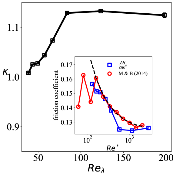
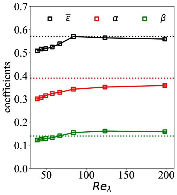
Figure 1: (a) Amplitude of mean velocity profile, $\kappa$ in Eq. 7, as function of $Re_{\lambda}$. The inset panel shows the dependence of the friction coefficient ($f$) on $Re^{*}$ (blue), in comparison with the result obtained by Musacchio and Boffetta (2014) (red). The dashed black line in the inset panel shows the curve of $f=0.124+5.75/Re^{*}$, which fits the red dots in the large $Re^{*}$ range Musacchio and Boffetta (2014). (b) The global dissipation rate ($\overline{\epsilon}$) and the coefficients obtained by fitting the profiles of kinetic energy, $\alpha$ and $\beta$ in Eq. 10, as function of $Re_{\lambda}$. The horizontal dotted red and green lines represent the values $\alpha=0.391$ and $\beta=0.138$, respectively, obtained by Borue and Orszag (1996). The horizontal black dotted line represents the global dissipation rate (expressed in the dimensionless form used in this work) reported by Musacchio and Boffetta (2014) for $Re^{*}=2000$.

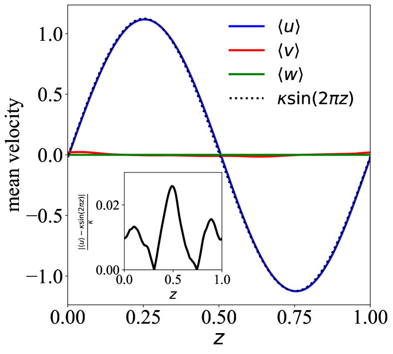
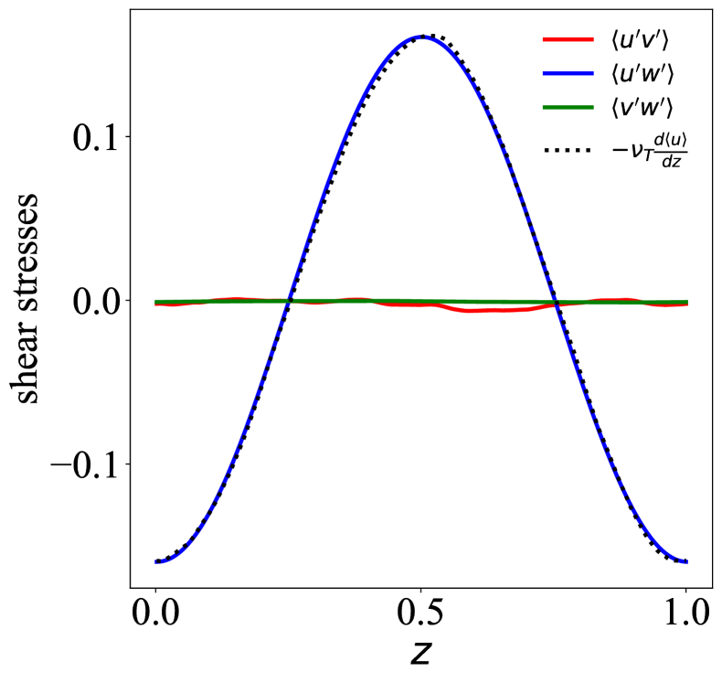
Figure 2: (a) The adimensional mean quantities of each component of the velocity of Run 8. The only non-zero term is $\langle u\rangle$, having a maximum value of $\kappa$, where $\kappa=1.12$. The black dotted line shows the curve of $\kappa\sin(2\pi z)$. The inset plot shows the deviation of $\langle u\rangle$ from $\kappa\sin(2\pi z)$ estimated by $\frac{|\langle u\rangle-\kappa\sin(2\pi z)|}{\kappa}$. (b) The different adimensional shear stress terms of Run 8. The only non-zero term is $\langle u^{\prime}w^{\prime}\rangle$, whose $z$ dependence is given by relation (8). The black dotted line shows the function $-\nu_{T}\frac{d\langle u\rangle}{dz}$, where $\nu_{T}=0.023$ is the turbulent viscosity (Eq. (14)) for the Run 8.

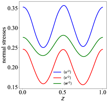
(a) $Re_{\lambda}=38.7$

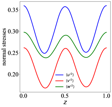
(b) $Re_{\lambda}=49.3$

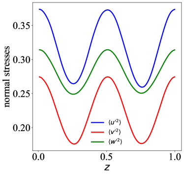
(c) $Re_{\lambda}=66.9$

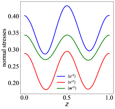
(d) $Re_{\lambda}=123.4$

Figure 3: The different normal stresses with $\langle u^{\prime 2}\rangle>\langle w^{\prime 2}\rangle>\langle v^{\prime 2}\rangle$. The $z$-dependence is given by the fits of equation (9).

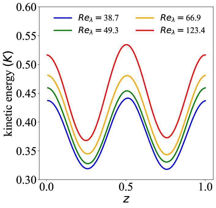
Figure 4: The mean kinetic energy profile $K(z)=\frac{1}{2}\langle u_{i}u_{i}\rangle$ for different Reynolds numbers.

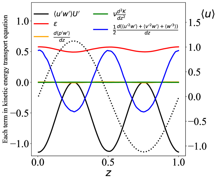
Figure 5: The amplitudes of the terms of the kinetic energy transport equation (11) for Run 7. The mean velocity profile is also shown as dotted line, for reference.

II.3 Kinetic energy balance equation

We next consider the kinetic energy balance equation, givingBernard and Wallace (2002):

$$0= \tau U^{\prime}(z)-\epsilon-\frac{1}{\rho}<p^{\prime}w^{\prime}>+\nu\frac{d^{2}K}{dz^{2}}$$ (11)

$$- \frac{d}{dz}\left(<w^{\prime}u^{\prime 2}>+<w^{\prime}v^{\prime 2}>+<w^{\prime 3}>\right)$$

where the different terms represent respectively the production of kinetic energy, the dissipation, the pressure work, the viscous transport and turbulent transport. These terms have been computed for run 7, and are shown in figure 5. It is visible first that the viscous transport and pressure works are negligible compared to other terms. There is a balance between production and dissipation added to turbulent transport. The dissipation is almost constant, with a small modulation, as already noticed in previous worksMusacchio and Boffetta (2014). The production is close to 0 at two positions corresponding to vanishing velocity shears. At these positions, the kinetic energy is minimum (see figure 4) and also its transport is negative. The production is larger for strong shear zones, where the mean velocity shear is the larger. At these positions, the turbulent transport is also the larger.

III Expression of the Reynolds stress onto a tensor basis

In this section we aim at deriving a relation expressing the Reynolds stress in terms of the gradients of the mean velocity flow. Such a relation, also known as turbulence closure equation, allows to have a self-contained model for the description of the mean flow. To this end, we introduce the Reynolds stress tensor defined as $\mathbf{T}=-\langle\mathbf{u^{\prime}}\otimes\mathbf{u^{\prime}}\rangle$ (with $\otimes$ denoting the dyadic product). The anisotropic stress tensor is $\mathbf{R}=-\mathbf{T}+\frac{2}{3}K\mathbf{I}$, where $K$ is the kinematic energy and $\mathbf{I}$ is the identity tensor. The mean velocity gradient tensor $\mathbf{A}=\partial\langle u_{i}\rangle/\partial x_{j}$, and the mean strain-rate $\mathbf{S}$ and rotation-rate $\mathbf{W}$ tensors are also introduced as:

$$\mathbf{S} = \frac{1}{2}\left(\frac{\partial\langle u_{i}\rangle}{\partial x_{j}}+\frac{\partial\langle u_{j}\rangle}{\partial x_{i}}\right),$$ (12)

$$\mathbf{W} = \mathbf{A}-\mathbf{S}.$$ (13)

A closure for the turbulence equations corresponds to expressing the Reynolds stress tensor using mean quantities, e.g. when the closure is local, using the tensors $\mathbf{S}$ and $\mathbf{W}$. Below we first consider the simplest linear closure and estimate the eddy-viscosity, and later on we address a nonlinear expression using a quadratic constitutive equation.

III.1 Boussinesq’s eddy-viscosity hypothesis and its assessment

It is seen from equations (7) and (8) that the only non-zero non-diagonal term in the stress tensor has the same $z$-dependence as the mean gradient term. This leads to an eddy-viscosity of the form:

$$\nu_{T}=\frac{\tau}{U^{\prime}(z)}=\left(\frac{1}{(2\pi)^{2}\kappa}-\frac{1}{Re}\right).$$ (14)

The eddy-viscosity does not depend on $z$, but depend on the Reynolds number and the coefficient $\kappa$. The values of $\nu_{T}$ provided by this equation are shown in Table 1; these values are in agreement with results at comparable Reynolds numberMusacchio and Boffetta (2014) and imply that $\nu_{T}/\nu=O(10^{2})$. However, the estimation of an eddy-viscosity does not validate the linear closure. The Boussinesq’s hypothesis, which is at the basis of all eddy-viscosity turbulence models, corresponds to a linear proportionality between tensors Boussinesq (1877) :

$$\mathbf{R}=2\nu_{T}\mathbf{S}.$$ (15)

For the flow considered here, there are some symmetries so that the strain as well as the stress have a simplified form:

$$\mathbf{S}=\frac{a}{2}\left(\begin{array}[]{ccc}0&0&1\\ 0&0&0\\ 1&0&0\end{array}\right)$$ (16)

and

$$\mathbf{R}=\left(\begin{array}[]{ccc}\frac{2}{3}K-\sigma^{2}_{u}&0&\tau\\ 0\!&\frac{2}{3}K-\sigma^{2}_{v}&0\\ \tau&0&\frac{2}{3}K-\sigma^{2}_{w}\end{array}\!\right),$$ (17)

where $a=U^{\prime}(z)$, $\sigma^{2}_{u}=\langle u^{\prime 2}\rangle$ and the same for $\sigma^{2}_{v}$ and $\sigma^{2}_{w}$.

It is then clear, as also the case for turbulent channel flows Speziale (1987); Nisizima and Yoshizawa (1987); Pope (2000), that such linear relation between tensors can be realized only when diagonal terms are zero, i.e. in an isotropic situation. However, the Kolmogorov flow is anisotropic and as seen in figure 3, the three normal stresses are all different, which means that a precise proportionality does not exist. In such framework, eddy-viscosity models will only properly capture the shear stress component, and cannot represent the normal stresses. The relative importance of these different components is considered below by using an alignment indicator. For this, we consider the inner product between tensors: $\mathbf{A}:\mathbf{B}=\{\mathbf{A}^{t}\mathbf{B}\}=A_{ij}B_{ij}$, where $\{\mathbf{X}\}$ is a notation for the trace of $\mathbf{X}$. The norm is then $||\mathbf{A}||^{2}=\mathbf{A}:\mathbf{A}$. As a direct test of Boussinesq’s hypothesis, we first represent here the normalized inner product of ${\bf R}$ and ${\bf S}$ tensors (which is similar to the cosine of an “angle” between vectors, see Schmitt and Hirsch (2000); Schmitt (2007a)):

$$\rho_{RS}=\frac{\mathbf{R}:\mathbf{S}}{||\mathbf{R}||~{}||\mathbf{S}||}.$$ (18)

The ratio $\rho_{RS}$ is thus a number between $-1$ and $1$, which characterizes the validity of Boussinesq’s hypothesis: it is $1$ when this hypothesis is valid, and when close to $0$ it corresponds to the case of “orthogonal” tensors. The behaviour of this quantity is shown in figure 6. It is seen that a plateau close to the value one appears in certain regions; in particular the Boussinesq’s hypothesis is approximately valid when the mean velocity gradient is large, whereas it fails dramatically for some range of values around the positions where the mean velocity gradient vanishes.

More quantitatively, from Run 7, we find $\rho_{RS}=0.93$ for $z=1/2$ and by choosing a threshold value at $\rho_{RS}=0.9$, we find that $0.9\leq\rho_{RS}\leq 1$ for $z\in[0,0.13]\cup[0.39,0.59]\cup[0.87,1]$. Hence for about half of the volume (46$\%$) the linear relation between strain and stress tensor is approximately valid with $\rho_{RS}$ larger than 0.9, while for the rest of the flow such linear relation fails to a large extent.

Furthermore, by considering figure 5 providing the different energy transport terms, we see that Boussinesq’s hypothesis is closest to validity at positions where the turbulent production is larger, and is totally failing at positions where there is almost no production and a negative turbulent transport term, meaning that the local dissipation is the result of a transport of kinetic energy.

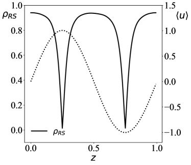
(a) $Re_{\lambda}=38.7$

(b) $Re_{\lambda}=49.3$

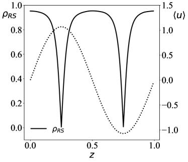
(c) $Re_{\lambda}=66.9$

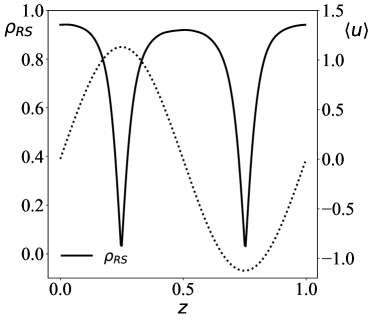
(d) $Re_{\lambda}=123.4$

Figure 6: Simulation results for the test of the validity of Boussinesq’s hypothesis, representing the alignment $\rho_{RS}$ between $\mathbf{R}$ and $\mathbf{S}$. The mean velocity profile is superposed in dotted line for reference.

III.2 A quadratic development for the Reynolds stress

We have seen above that the linear closure model cannot produce an anisotropic Reynolds stress tensor for anisotropic flows such as the Kolmogorov flow. Pope Pope (1975) has proposed to use the invariant theory in turbulence modeling, to represent the stress tensor as a development into a tensor basis composed of symmetric and traceless tensors expressed as polynomial based on the mean strain and rotation tensors. Originally it was on the form ${\bf R}=\sum_{i=1}^{10}a_{i}{\bf T}_{i}$ with $10$ basis tensors. By considering a quadratic development, only three tensors are used, which is complete for two dimensional flows Pope (1975), and is also a good approximation for fully 3-dimensional flows Jongen and Gatski (1998). As it was used for channel flows Schmitt (2007b); Modesti (2020) and for a tube bundle Wellinger et al. (2021), we propose here to use it also for the TKF.

In this framework, the anisotropic stress tensor writes as a three-terms development which is also a nonlinear constitutive equation:

$${\bf R}=a_{1}{\bf T}_{1}+a_{2}{\bf T}_{2}+a_{3}{\bf T}_{3},$$ (19)

where the three tensors of the basis are all symmetric and traceless Pope (1975):

$$\begin{array}[]{ll}{\bf T}_{1}={\bf S},&{\bf T}_{2}={\bf SW}-{\bf WS},\\ {\bf T}_{3}={\bf S}^{2}-\frac{1}{3}\eta_{1}{\bf I}\;\;.&\end{array}$$ (20)

The coefficients $a_{i}$ can be written using scalar invariants of the flow, which correspond to scalar fields whose values are independent of the system of reference. Invariants can be defined as the traces of different tensor products Spencer (1971). Some of the first invariants are the following: $\eta_{1}=\{{\bf S}^{2}\}$, $\eta_{2}=\{{\bf W}^{2}\}$, $\eta_{3}=\{{\bf S}^{3}\}$, $\eta_{4}=\{{\bf SW}^{2}\}$,$\eta_{5}=\{{\bf S}^{2}{\bf W}^{2}\}$, $\mu_{1}=\{{\bf R}^{2}\}$, $\mu_{2}=\{{\bf RS}\}$, $\mu_{3}=\{{\bf RSW}\}$, and $\mu_{4}=\{{\bf RS}^{2}\}$. All these invariants can be here estimated numerically. The coefficients $a_{1}$, $a_{2}$ and $a_{3}$ can be expressed using the above invariants by projecting the constitutive equation (equation (19)) onto the tensor basis: successive inner products of this equation with tensors ${\bf T}_{i}$ provides a system of scalar equations involving the invariants Jongen and Gatski (1998). For two-dimensional mean flows such as the KF, we have $\eta_{3}=0$ and $\eta_{5}=\eta_{1}\eta_{2}/2$, and the system of scalar equations is inverted to provide finally the quadratic constitutive equation using invariants:

$${\bf R}=\frac{\mu_{2}}{\eta_{1}}{\bf S}-\frac{\mu_{3}}{\eta_{1}\eta_{2}}{\bf T}_{2}+6\frac{\mu_{4}}{\eta_{1}^{2}}{\bf T}_{3}$$ (21)

where the invariants write for the TKF:

$$\eta_{1}=\frac{a^{2}}{2};\quad\eta_{2}=-\frac{a^{2}}{2};\quad\mu_{2}=a\tau$$ (22)

$$\mu_{3}=\frac{a^{2}}{4}\left(\sigma^{2}_{u}-\sigma^{2}_{w}\right),$$ (23)

$$\mu_{4}=\frac{a^{2}}{4}\left(\sigma^{2}_{v}-\frac{2}{3}K\right).$$ (24)

The two remaining tensors of the tensor basis are:

$$\mathbf{T}_{2}=\frac{a^{2}}{2}\left(\begin{array}[]{ccc}-1&0&0\\ 0&0&0\\ 0&0&1\end{array}\right)$$ (25)

and

$$\mathbf{T}_{3}=\frac{a^{2}}{12}\left(\begin{array}[]{ccc}1&0&0\\ 0&-2&0\\ 0&0&1\end{array}\right).$$ (26)

The quadratic constitutive equation finally writes, replacing invariants in equation (21):

$${\bf R}=\frac{2\tau}{a}{\bf S}+\left(\sigma^{2}_{u}-\sigma^{2}_{w}\right)\frac{1}{a^{2}}{\bf T}_{2}+\left(6\sigma^{2}_{v}-4K\right)\frac{1}{a^{2}}{\bf T}_{3}.$$ (27)

Equation (27) is a quadratic constitutive equation which expresses a nonlinear closure of the turbulent Kolmogorov flow; the first constant coefficient is twice the eddy-viscosity ($\tau/a=\nu_{T}$), whereas the other coefficients are space-dependent. Such expression belongs to nonlinear-eddy viscosity models (NEVM) Pope (1975); Speziale (1987); Nisizima and Yoshizawa (1987); it is also related with another well-known family of models called explicit algebraic Reynolds-stress models (EARSM), which are based on slightly different assumptions Gatski and Speziale (1993); Xu and Speziale (1996); Girimaji (1996); Wallin and Johansson (2000).

Equation (27) can also be seen as a mathematically simple relation, obtained from a projection onto a three tensor basis; however, even if mathematically simple, it provides new and interesting information on the relative importance of the different terms of this tensorial development according to the position considered. In NEVM and EARSM, the coefficients of such nonlinear development are expressed using other quantities such as e.g. $K$ and $\epsilon$, which are computed in the domain considered using transport equations Gatski and Rumsey (2002). Here we are not building such a model but the assessment of the relative importance of each term in the development will be useful for modelling studies.

When $a=U^{\prime}(z)\simeq 0$, for $z\simeq 1/4$ and $z\simeq 3/4$, $\cos(2\pi z)=0$ and all ${\bf S}$, ${\bf T}_{2}$ and ${\bf T}_{3}$ vanish, but in the three-terms development of ${\bf R}$, the second term and the third are non-zero constants, since the coefficients diverge (the $a^{2}$ terms cancel). In those positions, we see that ${\bf R}$ is a diagonal tensor which is not vanishing: figure 7 shows that the second term is also very small and that the third term is dominant. This means that in those positions, the Boussinesq’s linear eddy-viscosity approximation is no longer appropriate and the anisotropic stress tensor is a constant perpendicular to the linear term and approximately proportional to ${\bf T}_{3}={\bf S}^{2}-\frac{1}{3}\eta_{1}{\bf I}$. We have also noted above that at those positions, the production of kinetic energy is very small and the kinetic energy dissipation at those positions is produced elsewhere and transported.

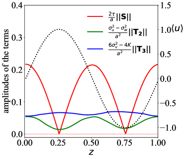
(a) $Re_{\lambda}=38.7$

(b) $Re_{\lambda}=49.3$

(c) $Re_{\lambda}=66.9$

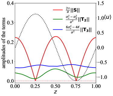
(d) $Re_{\lambda}=123.4$

Figure 7: The amplitudes of the terms at the right hand side of Eq. (27) as function of $z$. The mean velocity profile is also represented as a dotted line, for reference. The horizontal red dotted lines mark the 0 value for the amplitudes. The simulation results of Run 1, 3, 5, 7 are shown here.

IV Periodic flow with non-sinusoidal forcing

As we have seen, the Kolmogorov flow, in its original definition, is sustained by a monochromatic sinusoidal forcing. The resulting mean flow profile is also sinusoidal with the same shape of the force term, both in laminar and in turbulent flow conditions. This peculiar property is of great help in the analysis of the turbulent flow and, as we have seen, it simplifies the formulation of a closure relation. It is therefore of interest to ask what happens when the shape of the force is changed to other periodic or quasi-periodic shapes Romanò (2021). Here we investigate a forcing having a Gaussian shape. Although this function is non-periodic and has an unbounded support, one can adjust its width in such a way that its value and its derivative becomes sufficiently small at the borders. Furthermore, the Gaussian has the advantage to be easily implemented in spectral space. Here we test only one given Reynolds number, as this is sufficient to contrast the qualitative differences with the sinusoidal forcing case. The dimensionless viscosity for this case are $0.00063$, the same as the Run 4 with sinusoidal forcing, while the Taylor based Reynolds number is $44.1$.

The Gaussian-type forcing is of the form of:

$$\mathbf{f}=(A\exp\left(-\frac{(z-0.5)^{2}}{2\ell^{2}}\right)+C)\mathbf{e}_{x},$$ (28)

where $A$ is the forcing parameter, $C$ is a constant to make $\overline{\mathbf{f}}=0$ in equation (1) and $\ell=0.1$ (in $H$ units), which is equivalent to the standard deviation, and controls the width of the Gaussian shape.

Figure 8 shows the Reynolds stress components: the shear stress and normal stresses. The normal stresses have a shape that can not be fitted with known functions and only the numerical result is shown here. It is visible that normal stresses are again anisotropic, with $\sigma_{u}^{2}>\sigma_{w}^{2}>\sigma_{v}^{2}$ at all positions. The shear stress $\tau=-\langle u^{\prime}w^{\prime}\rangle$ is as in the TKF the only non-zero shear stress, and is proportional to $U^{\prime}(z)$, with a coefficient $\nu_{T}=0.016$ (it was found of the same order, $0.0236$, in Run 4 wih sinusoidal forcing according to Eq. (14)).

This shows that here also the eddy-viscosity is a constant, as was found for the sinusoidal forcing. From equation (6), introducing this numerical result $\tau=\nu_{T}U^{\prime}(z)$ we obtain

$$U^{\prime\prime}(z)=-\frac{Re}{\nu_{T}/\nu+1}\mathbf{f}.$$ (29)

This shows that the mean velocity profile is proportional to twice the integral of the forcing. The primitive of the Gaussian is non-analytical and involves the error function; it can be estimated numerically, as shown in figure 9. An excellent superposition is found. The shape of the mean velocity is still Gaussian-like, but its precise analytical expression is given by the function whose second derivative is a Gaussian.

The alignment between the tensors of ${\bf R}$ and ${\bf S}$ (as defined in Eq. (18)) is also examined for the case with Gaussian forcing, as shown in Fig. 10. We observe also in this case the plateaus obtained at the position where the mean velocity gradient is large. Qualitatively, we find that $0.9\leq\rho_{RS}\leq 1$ for $z\in[0.12,0.4]\cup[0.6,0.88]$, corresponding totally to about $56\%$ of the considered domain.

Next, the quadratic development given by equation (27) is tested and shown in figure 11. It is seen that the linear term is dominant in part of the domain, and vanishes at the central position, where the mean velocity is null; in this position the two nonlinear terms do not vanish. Globally all three terms are needed to achieve the closure of the stress tensor.

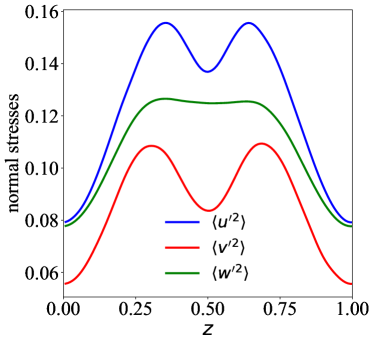
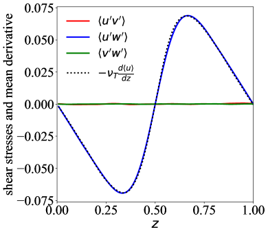
Figure 8: (a) The normal stresses; (b) The shear stresses and the function of $-\nu_{T}\frac{d\langle u\rangle}{dz}$ (black dotted line), where $\nu_{T}$ is the turbulent viscosity (Eq. (14)) and numerically found as $0.016$ here, for the case with Gaussian forcing (same parameters with Run 4).

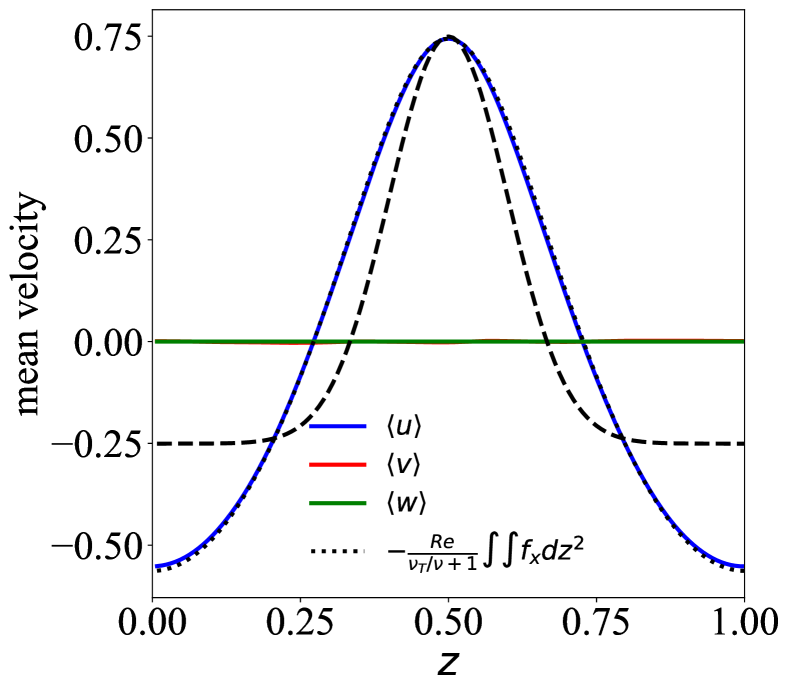
Figure 9: Comparison of the mean profile ($\langle u\rangle$, blue solid line) and the double integral of the forcing (black dotted line) for the case with Gaussian forcing (same parameters with Run 4). The coefficient of $\frac{Re}{\nu_{T}/\nu+1}$ is numerically found as 61.27. The black dashed line represents the Gaussian profile forcing (28). The profiles of $\langle v\rangle$ and $\langle w\rangle$ are very close to zero and almost superposed.

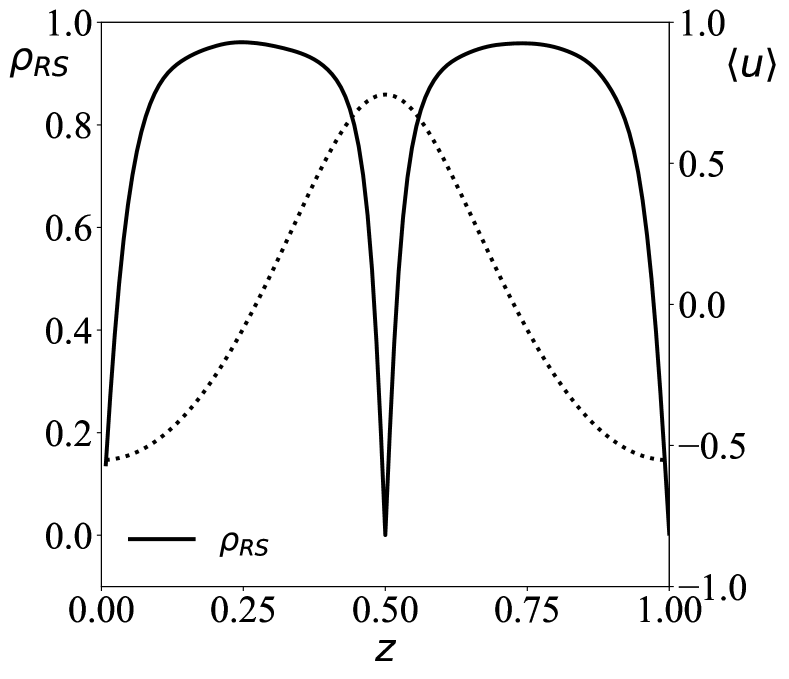
Figure 10: Estimation of the alignment $\rho_{RS}$ between $\mathbf{R}$ and $\mathbf{S}$, for the case with Gaussian forcing (same parameters with Run 4). The mean velocity profile is superposed in dotted line for reference.

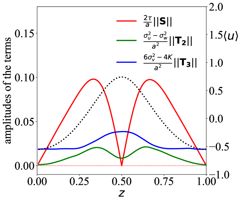
Figure 11: The amplitudes of the terms at the right hand side of Eq. (27) as function of $z$ for the case with Gaussian forcing (same parameters with Run 4). The mean velocity profile is also represented as a dotted line, for reference. The horizontal red dotted lines mark the 0 value for the amplitudes.

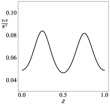
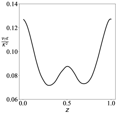
Figure 12: The adimensional mean quantities of $\frac{\nu_{T}\epsilon}{K^{2}}$ of (a) Run 7 and (b) the case with Gaussian forcing.

V Conclusion

We have considered here the closure relation for the Reynolds stress in a numerically simulated turbulent Kolmogorov flow. As the simplest realization of turbulence with a spatially dependent mean flow, such model system is a convenient test ground for turbulent transport models. With a forcing of the form $\sin(2\pi z)$, it was found that the mean velocity profile has the same form, with a damping of a factor $\kappa$ with respect to the mean velocity value calculated from forcing terms. The value of $\kappa$ was found to increase with the Reynolds number, and of the order of 1.01 to 1.12 for the range of Reynolds numbers considered here. The only non-zero shear stress term is proportional to $\cos(2\pi z)$ as expected, and the normal stress components all involve a square cosine expression of the form $\alpha+\beta\cos^{2}(2\pi z/H)$, where the parameters $\alpha$ and $\beta$ are numerically estimated and found to saturate for the largest Reynolds numbers considered here. The normal stresses, i.e. $\langle u^{\prime 2}\rangle,\langle w^{\prime 2}\rangle,\langle v^{\prime 2}\rangle$, are all different in amplitude, showing that the turbulence is anisotropic.

It was also shown that a quadratic nonlinear constitutive equation can be proposed for this flow. Specifically a linear term and two nonlinear terms in the form of traceless and symmetric tensors ${\bf SW}-{\bf WS}$ and ${\bf S}^{2}-\frac{1}{3}\{{\bf S}^{2}\}{\bf I}$ are involved and their coefficients are here numerically estimated. For about half of the flow domain, the linear term is dominating, whereas for the vanishing mean velocity regions a constant term is the only one remaining. Hence an effective viscosity coefficient can indeed be estimated for the Kolmogorov flow, but contrary to what has been indicated previously Rollin, Dubief, and Doering (2011) this type of turbulence without boundaries does not generate an effective diffusion of momentum, since nonlinear terms are needed: globally all linear and nonlinear terms are needed for the complete Reynolds stress closure.

The values obtained here are in agreement with previous works Borue and Orszag (1996); Musacchio and Boffetta (2014). Using 8 different runs with different grid sizes from $128^{3}$ to $512^{3}$, and with Reynolds numbers from $Re_{\lambda}=39$ to $198$, the Reynolds number dependence of involved parameters has been checked with expected convergence toward the largest Reynolds number considered.

Finally a periodic flow with non-sinusoidal forcing has been considered, with the choice of a Gaussian shape. It was found that the shear stress term $\tau$ is proportional to the mean velocity derivative, indicating that for such forcing also the eddy-viscosity does not depend on $z$. With such numerical result, we obtain that the mean velocity profile is twice the integral of the forcing. The shape of the normal stresses in this case is non-trivial and can not be precisely fitted. A quadratic development of the constitutive equation can also be proposed for this flow.

We may qualitatively compare here the turbulent flows sustained by the sinusoidal forcing (TKF) and the Gaussian forcing. In both cases the eddy-viscosity is found to be constant. We observe that the relation stating that $U^{\prime\prime}$ is proportional to the forcing (29), is in fact also valid for the TKF case. Such constant eddy-viscosity found here for two very different types of forcing is not to be taken as a coincidence: we hypothesize here that this is a general property of such boundary free periodic flows. We shall note here that for such flows the classical expression of the eddy-viscosity $\nu_{T}=C_{\mu}k^{2}/\epsilon$ does not hold, as demonstrated in Figure 12 plotting $\frac{\nu_{T}\epsilon}{K^{2}}$ for Run 7 and Gaussian forcing cases, showing that $C_{\mu}$ is not a constant for both flows. There are however, two main differences between the two forcing cases. The first lies in the shape of the mean velocity profile. For the TKF, since the second integral of the forcing is proportional to the forcing, equation (29) directly gives the mean velocity profile, as being proportional to the forcing. In the Gaussian forcing case, the mean velocity is a non-analytical function, obtained as the second integral of the Gaussian. The second difference is in the shape of normal stresses, whose expression could be fitted using $\cos^{2}$ terms for the TKF, while no known analytical fit for the Gaussian forcing is available.

It is also worth mentioning that the linear or non-linear eddy-viscosity modelling that were considered in this work all rely on a local expression of the velocity, through derivatives of the mean velocity field. Such local expression is known to be incomplete Tennekes and Lumley (1972); Corrsin (1975); Pope (2000) and non-local models have been proposed, based on space and time integrations of velocity gradients Hinze, Sonnenberg, and Builtjes (1974); Hamba (2005), as reviewed and discussed in a recent book Egolf and Hutter (2020).

As a perspective let us mention the recent work Bos (2020) describing a flow behind a grid in a wind tunnel as having locally, close to the grid, sinusoidal variations. This could provide ideas to perform measurements of a TKF and to check experimentally the closure proposed in the present study. A more systematic numerical study of non-sinusoidal forcing in future work may also help to provide a general expression for normal stresses, which would be valid for all kind of forcing. It remains also to be understood from analytical arguments why the eddy-viscosity does not depend on $z$ for such periodic flow, contrary to what is found in similar bounded flow such as the channel flow Schmitt (2007b) or the boundary-layer flow.

Data Availability Statement

Data available on request from the authors.

Conflict of interest

The authors have no conflicts to disclose.

References

- Meshalkin and Sinai (1961) L. D. Meshalkin and I. G. Sinai, “Investigation of the stability of a stationary solution of a system of equations for the plane movement of an incompressible viscous liquid,” J. Appl. Math. Mech. 25, 1700–1705 (1961).
- Green (1974) J. S. A. Green, “Two-dimensional turbulence near the viscous limit,” J. Fluid Mech. 62, 273–287 (1974).
- Bondarenko, Gak, and Dolzhanskii (1979) N. F. Bondarenko, M. Z. Gak, and F. V. Dolzhanskii, “Laboratory and theoretical models of plane periodic flow,” Akademiia Nauk SSSR, Izvestiia, Fizika Atmosfery i Okeana 15, 1017–1026 (1979).
- Obukhov (1983) A. M. Obukhov, “Kolmogorov flow and laboratory simulation of it,” Russ. Math. Surv. 38, 113–126 (1983).
- Kliatskin (1972) V. I. Kliatskin, “On the nonlinear theory of stability of periodic flows,” J. Appl. Math. Mech. 36, 243–250 (1972).
- Borue and Orszag (1996) V. Borue and S. A. Orszag, “Numerical study of three-dimensional Kolmogorov flow at high Reynolds numbers,” J. Fluid Mech. 306, 293–323 (1996).
- Shebalin and Woodruff (1997) J. V. Shebalin and S. L. Woodruff, “Kolmogorov flow in three dimensions,” Phys. Fluids 9, 164–170 (1997).
- Biferale and Toschi (2001) L. Biferale and F. Toschi, “Anisotropic homogeneous turbulence: hierarchy and intermittency of scaling exponents in the anisotropic sectors,” Phys. Rev. Lett. 86, 4831 (2001).
- Balmforth and Young (2002) N. J. Balmforth and Y.-N. Young, “Stratified Kolmogorov flow,” J. Fluid Mech. 450, 131 (2002).
- Boffetta et al. (2005) G. Boffetta, A. Celani, A. Mazzino, A. Puliafito, and M. Vergassola, “The viscoelastic Kolmogorov flow: eddy viscosity and linear stability,” J. Fluid Mech. 523, 161 (2005).
- Musacchio and Boffetta (2014) S. Musacchio and G. Boffetta, “Turbulent channel without boundaries: The periodic Kolmogorov flow,” Phys. Rev. E 89, 023004 (2014).
- Rollin, Dubief, and Doering (2011) B. Rollin, Y. Dubief, and C. R. Doering, “Variations on Kolmogorov flow: turbulent energy dissipation and mean flow profiles,” J. Fluid Mech. 670, 204 (2011).
- She (1987) Z. S. She, “Metastability and vortex pairing in the Kolmogorov flow,” Phys. Lett. A 124, 161–164 (1987).
- Berti and Boffetta (2010) S. Berti and G. Boffetta, “Elastic waves and transition to elastic turbulence in a two-dimensional viscoelastic Kolmogorov flow,” Phys. Rev. E 82, 036314 (2010).
- Chandler and Kerswell (2013) G. Chandler and R. Kerswell, “Invariant recurrent solutions embedded in a turbulent two-dimensional kolmogorov flow,” J. Fluid Mech. 722, 554–595 (2013).
- Lucas and Kerswell (2014) D. Lucas and R. R. Kerswell, “Spatiotemporal dynamics in two-dimensional Kolmogorov flow over large domains,” J. Fluid Mech. 750, 518–554 (2014).
- Lucas and Kerswell (2015) D. Lucas and R. R. Kerswell, “Recurrent flow analysis in spatiotemporally chaotic 2-dimensional Kolmogorov flow,” Phys. Fluids 27, 045106 (2015).
- Pope (2000) S. B. Pope, Turbulent flows (Cambridge University Press, 2000).
- Schmitt (2007a) F. G. Schmitt, “About boussinesq’s turbulent viscosity hypothesis: historical remarks and a direct evaluation of its validity,” Comptes Rendus Mécanique 335, 617–627 (2007a).
- Schmitt (2007b) F. G. Schmitt, “Direct test of a nonlinear constitutive equation for simple turbulent shear flows using dns data,” Communications in Nonlinear Science and Numerical Simulation 12, 1251–1264 (2007b).
- Hou and Li (2007) T. Y. Hou and R. Li, “Computing nearly singular solutions using pseudo-spectral methods,” J. Comput. Phys. 226, 379–397 (2007).
- Sarris et al. (2007) I. E. Sarris, H. Jeanmart, D. Carati, and G. Winckelmans, “Box-size dependence and breaking of translational invariance in the velocity statistics computed from three-dimensional turbulent Kolmogorov flows,” Phys. Fluids 19, 095101 (2007).
- Bernard and Wallace (2002) P. Bernard and J. Wallace, Turbulent flow: analysis, measurement, and prediction (John Wiley & Sons, 2002).
- Boussinesq (1877) J. Boussinesq, Essai sur la théorie des eaux courantes (Mémoires présentés par divers savants à l’Académie des Sciences vol. XXIII, Imprimerie Nationale, 1877).
- Speziale (1987) C. G. Speziale, “On nonlinear kl and k- models of turbulence,” J. Fluid Mech. 178, 459–475 (1987).
- Nisizima and Yoshizawa (1987) S. Nisizima and A. Yoshizawa, “Turbulent channel and couette flows using an anisotropic k-epsilon model,” AIAA J. 25, 414–420 (1987).
- Schmitt and Hirsch (2000) F. G. Schmitt and C. Hirsch, “Experimental study of the constitutive equation for an axisymmetric complex turbulent flow,” ZAMM/Zeitschrift für Angewandte Mathematik und Mechanik 80, 815–825 (2000).
- Pope (1975) S. B. Pope, “A more general effective-viscosity hypothesis,” J. Fluid Mech. 72, 331–340 (1975).
- Jongen and Gatski (1998) T. Jongen and T. B. Gatski, “General explicit algebraic stress relations and best approximation for three-dimensional flows,” Int. J. Eng. Sci. 36, 739–763 (1998).
- Modesti (2020) D. Modesti, “A priori tests of eddy viscosity models in square duct flow,” Theor. Comput. Fluid Dyn. 34, 713–734 (2020).
- Wellinger et al. (2021) P. Wellinger, P. Uhl, B. Weigand, and J. Rodriguez, “Analysis of turbulence structures and the validity of the linear boussinesq hypothesis for an infinite tube bundle,” International Journal of Heat and Fluid Flow in press, 108779 (2021).
- Spencer (1971) A. J. M. Spencer, “Part iii. theory of invariants,” Continuum Phys. 1, 239–353 (1971).
- Gatski and Speziale (1993) T. Gatski and C. Speziale, “On explicit algebraic stress models for complex turbulent flows,” J. Fluid Mech. 254, 59–78 (1993).
- Xu and Speziale (1996) X.-H. Xu and C. Speziale, “Explicit algebraic stress model of turbulence with anisotropic dissipation,” AIAA J. 34, 2186–2189 (1996).
- Girimaji (1996) S. S. Girimaji, “Fully explicit and self-consistent algebraic reynolds stress model,” Theoretical and Computational Fluid Dynamics 8, 387–402 (1996).
- Wallin and Johansson (2000) S. Wallin and A. V. Johansson, “An explicit algebraic reynolds stress model for incompressible and compressible turbulent flows,” Journal of Fluid Mechanics 403, 89–132 (2000).
- Gatski and Rumsey (2002) T. Gatski and C. Rumsey, “Closure strategies for turbulent and transitional flows,” (Cambridge University Press, 2002) Chap. Linear and nonlinear eddy viscosity models, pp. 9–46.
- Romanò (2021) F. Romanò, “Stability of generalized kolmogorov flow in a channel,” Phys. Fluids 33, 024106 (2021).
- Tennekes and Lumley (1972) H. Tennekes and J. Lumley, A first course in turbulence (MIT press, 1972).
- Corrsin (1975) S. Corrsin, “Limitations of gradient transport models in random walks and in turbulence,” Adv. geophys. 18, 25–60 (1975).
- Hinze, Sonnenberg, and Builtjes (1974) J. Hinze, R. Sonnenberg, and P. Builtjes, “Memory effect in a turbulent boundary-layer flow due to a relatively strong axial variation of the mean-velocity gradient,” Appl. Sci. Res. 29, 1–13 (1974).
- Hamba (2005) F. Hamba, “Nonlocal analysis of the reynolds stress in turbulent shear flow,” Phys. Fluids 17, 115102 (2005).
- Egolf and Hutter (2020) P. Egolf and K. Hutter, Nonlinear, nonlocal and fractional turbulence (Springer, 2020).
- Bos (2020) W. T. Bos, “Production and dissipation of kinetic energy in grid turbulence,” Phys. Rev. Fluids 5, 104607 (2020).