CobBO: Coordinate Backoff Bayesian Optimization with Two-Stage Kernels

Abstract

Bayesian optimization is a popular method for optimizing expensive black-box functions. Yet it oftentimes struggles in high dimensions where the computation could be prohibitively heavy. While a complex kernel with many length scales are prone to overfitting and expensive to train, a simple kernel with too few length scales cannot effectively capture the variations of the high dimensional function in different directions. To alleviate this problem, we introduce Coordinate backoff Bayesian Optimization (CobBO) with two-stage kernels. During each round, the first stage uses a simple coarse kernel that sacrifices the approximation accuracy for computational efficiency. It captures the global landscape by purposely smoothing away local fluctuations. Then, in the second stage of the same round, past observed points in the full space are projected to the selected subspace to form virtual points. These virtual points, along with the means and variances of their unknown function values estimated using the simple kernel of the first stage, are fitted to a more sophisticated kernel model in the second stage. Within the selected low dimensional subspace, the computational cost of conducting Bayesian optimization therein becomes affordable. To further enhance the performance, a sequence of consecutive observations in the same subspace are collected, which can effectively refine the approximation of the function. This refinement lasts until a stopping rule is met determining when to back off from a certain subspace and switch to another. This decoupling significantly reduces the computational burden in high dimensions, which fully leverages the observations in the whole space rather than only relying on observations in each coordinate subspace. Extensive evaluations show that CobBO finds solutions comparable to or better than other state-of-the-art methods for dimensions ranging from tens to hundreds, while reducing both the trial complexity and computational costs.

1 Introduction

Bayesian optimization (BO) has emerged as an effective zero-order paradigm for optimizing expensive black-box functions. It has been widely used in various real applications, e.g., parameter tuning for recommendation systems, automatic database configuration tuning, and simulation-based optimization.

Though highly competitive in low dimensions (e.g., the dimension $D\leq 20$ Frazier (2018)), Bayesian optimization based on Gaussian Process (GP) regression has obstacles in high dimensions.
Curse of dimensionality: As a sample efficient method, Bayesian optimization often suffers from high dimensions. Fitting the GP model (estimating the parameters, e.g., length scales Eriksson et al. (2019)) and optimizing the acquisition function all incur large computational costs in high dimensions. It also results in statistical insufficiency of exploration Djolonga et al. (2013); Wang et al. (2017). As the GP regression’s error grows with dimensions Bull (2011), more samples are required to balance that in high dimensions, which could cubically increase the computational costs in the worst case Mutny & Krause (2018). Undesirably, the computation times, especially for model fitting and acquisition function optimization, could be even far longer than the required time for evaluating the function values in high dimensions, which significantly limits the application.
Multiple length scales: The smoothness of the regression is determined by the specified kernel and the corresponding length scales, where the latter can be viewed as the measuring units along different coordinates. The landscapes of the function on the global full space and on different local coordinate subspaces can vary significantly as BO tries to approximate all of them in each iteration using a family of Gaussian functions. Thus, a single kernel with a fixed set of length scales cannot effectively fit all.

Algorithm 1 High level description of CobBO

1:  for each round $r$ do

2:     Stage 1:

3:     GP regression using a computation-efficient kernel $K_{1}$ on all of the observed data points from the full space $\Omega$

4:     Select a subspace $\Omega_{r}$, construct “virtual points” and estimate the means (and optional variances) of their function values using $K_{1}$

5:     Stage 2:

6:     repeat

7:        BO on the same subspace $\Omega_{r}$ with a sophisticated and maybe time-consuming kernel $K_{2}$ using both the “virtual points” and truly observed ones on $\Omega_{r}$

8:     until backoff stopping rule is met

9:  end for

10:  return the best observed data point

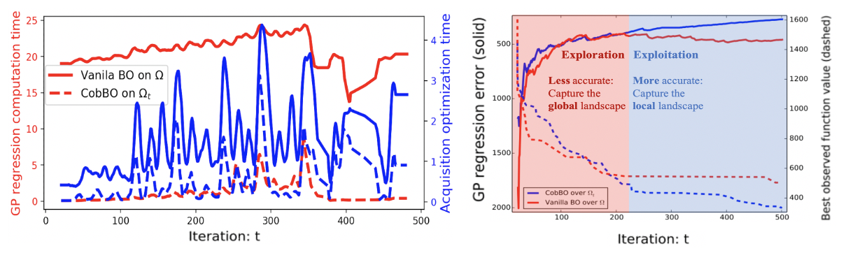
Figure 1: Minimize the fluctuated Rastrigin function on $[-5,10]^{50}$ with $20$ initial samples. [Left] Computation times for training the GP regression model and maximizing the acquisition function at each iteration. CobBO significantly reduces the execution time compared with a vanilla BO, e.g. $\times 13$ faster in this case. [Right] The average error between the GP predictions before making queries and the true function values at the queried points (solid curves, the higher the better) and the best observed function value (dashed curves, the lower the better) at iteration $t$. During each round, CobBO captures the global landscape less accurately using the RBF kernel at the first stage, and then explores selected subspaces $\Omega_{t}$ more accurately using the Matern kernel at the second stage. This eventually better exploits the promising subspaces.

To alleviate, we introduce two-stage kernels and design coordinate backoff Bayesian optimization (CobBO), as illustrated in Algorithm 1. The first stage uses a computation-efficient kernel for capturing the global landscape in the full space. For example, one can use a simple and coarse kernel to purposely smooth away local fluctuations, e.g., RBF Radial basis function , where efficient algorithms in $O(N\log N)$ for $N$ observations have been well studied Gumerov & Duraiswami (2007). In contrast, the second stage utilizes a more sophisticated kernel, e.g., the Automatic Relevance Determination (ARD) Matérn 5/2 Rasmussen & Williams (2005), that learns the varying length scales to properly capture the local fluctuations in the selected subspaces.

To bridge the two stages, CobBO introduces virtual points in the first stage by estimating the values of the unobserved points from the queried ones projected to selected promising subspaces. Then it conducts BO by conditioning on both virtual points and real observations that reside in the selected subspace, by which the information outside the subspace can also be effectively utilized. This introduced decoupling allows us to apply two different kernels on the global space and the subspace, respectively. It can dramatically reduce both the model fitting time in the full space and the acquisition function optimization time in the subspace, as shown in Fig 1.

This method can be viewed as a variant of block coordinate ascent tailored to Bayesian optimization. While similar works exist Li et al. (2017); Moriconi et al. (2020); Oliveira et al. (2018), CobBO differs by introducing the two-stage kernels and the following features:

1. To refine the approximation in a subspace and also reduce the computation time, the second stage of CobBO relies on a sequence of observations determined by a stopping rule that backs off from a certain subspace and switches to another one. When consecutively querying data points in the same subspace, CobBO does not need to conduct the first-stage, including the model fitting and the GP regression, in the full space. In addition, in the second-stage on a low dimensional subspace, both computing the Gaussian process posterior and optimizing the acquisition function can be efficiently conducted, moderating the curse of dimensionality. However, querying a certain subspace comes at the expense of exploring other coordinate blocks. Yet prematurely shifting to different subspaces does not fully exploit the full potential of a given subspace. Hence determining the number of consecutive function queries within a subspace makes a trade-off between exploration and exploitation.

2. Selecting a block of coordinates requires determining the block size as well as the coordinates therein. CobBO selects the coordinate subsets by a multiplicative weights update method Arora et al. (2012) to the preference probability associated with each coordinate. Thus, it samples more promising subspaces with higher probabilities.

Through comprehensive evaluations, CobBO demonstrates appealing performance for dimensions ranging from tens to hundreds. It obtains comparable or better solutions with fewer queries, in comparison with the state-of-the-art methods, for most of the problems tested in Section 4.2.

2 Related work

Certain assumptions are often imposed on the latent structure in high dimensions. Typical assumptions include low dimensional embedding and additive structures. Their advantages manifest on problems with a low dimension or a low effective dimension. However, these assumptions do not necessarily hold in practice, e.g., for non-separable functions without redundant dimensions.

Low dimensional embedding: The function $f$ is assumed to have a low effective dimension Kushner (1964); Tyagi & Cevher (2014), e.g., $f(x)=g(\Phi x)$ for a function $g(\cdot)$ and a matrix $\Phi$ of $d\times D,d<<D$. It essentially assumes that $f(x)$ does not change along certain directions. A variety of methods have been developed, including random embedding Djolonga et al. (2013); Wang et al. (2016); Munteanu et al. (2019); Binois et al. (2020); Letham et al. (2020), Hashing-enhanced Subspace BO (HeSBO) Munteanu et al. (2019), and Mahalanobis kernel ALEBO Letham et al. (2020). Since not all the real-world problems fit the low dimensional embedding structure, CobBO is designed to optimize functions without redundant dimensions. It exploits the subspace structure, independent of the dimensions. Though the embedding-based algorithms and CobBO are based on different assumptions, REMBO Wang et al. (2016) and ALEBO Letham et al. (2020) are compared with CobBO in Section 4.2.3.

Additive structure: A decomposition assumption is often made by $f(x)=\sum_{i=1}^{k}f^{(i)}\left(x_{i}\right)$, with $x_{i}$ defined over low-dimensional components. In this case, the effective dimensionality of the model is the largest dimension among all additive groups Mutny & Krause (2018), which is usually small. The Gaussian process is structured as an additive model Gilboa et al. (2013); Kandasamy et al. (2015). However, learning the unknown structure incurs a considerable computational cost Munteanu et al. (2019), and is not always applicable for non-separable functions.

Trust regions and subspaces: Trust region BO has been proven effective for high-dimensional problems. Within the local trust regions, many efficient methods have been applied, e.g., local Gaussian models (TurBO Eriksson et al. (2019)), adaptive search on a mesh grid (BADS Acerbi & Ma (2017)) or quasi-Newton local optimization (BLOSSOM McLeod et al. (2018)). TurBO Eriksson et al. (2019) uses Thompson sampling to allocate samples across multiple regions. A related method is to use space partitions, e.g., LA-MCTSWang et al. (2020) on a Monte Carlo tree search algorithm to learn efficient partitions. CobBO differs by selecting low dimensional subspaces. A closely related work is LineBO Kirschner et al. (2019), which also significantly reduces the acquisition function optimization time by restricting on one-dimensional subspaces. However, as it uses a single kernel, it does not address the computational issue of the GP regression in the full space. See a comparison in Section 4.2.4.

3 Algorithm

Without loss of generality, suppose that the goal is to solve $x^{\ast}=\textrm{argmax}_{x\in\Omega}f(x)$ for a black-box function $f:{\Omega}\to\mathbb{R}$. The domain is normalized ${\Omega}=[0,1]^{D}$ with the coordinates indexed by $I=\{1,2,\cdots,D\}$. For a sequence of points $\mathcal{X}_{t}=\{x_{1},x_{2},\cdots,x_{t}\}$ with $t$ indexing the most recent iteration, we observe $\mathcal{H}_{t}=\left\{\left(x_{i},y_{i}=f(x_{i})\right)\right\}_{i=1}^{t}$. A subset $C_{t}\subseteq I$ of the coordinates is selected, forming a subspace $\Omega_{t}\subseteq\Omega$.

GP regression assumes a class of random functions in a probability space as surrogates that iteratively yield posterior distributions by conditioning on the queried points. For iteration $t$, instead of computing the Gaussian process posterior distribution $\left\{\hat{f}(x)\middle|\mathcal{H}_{t}=\left\{(x_{i},y_{i})\right\}_{i=1}^{t},x\in{\Omega}\right\}$ by conditioning on the observations $y_{i}=f(x_{i})$ at queried points $x_{i}$ in the full space $\Omega\subset\mathbb{R}^{D}$ for $i=1,\dots,t$, we change the conditional events, and consider

$$\left\{\hat{f}(x)\middle|R\left(P_{\Omega_{t}}(x_{1},\dots,x_{t}),\mathcal{H}_{t}\right),x\in{\Omega}_{t},{\Omega}_{t}\subset\Omega\right\}$$

for a projection function $P_{\Omega_{t}}(\cdot)$ to a random subspace ${\Omega}_{t}$ and an estimation function $R(\cdot,\cdot)$. The projection $P_{\Omega_{t}}(\cdot)$ maps the queried points to virtual points on a subspace ${\Omega}_{t}$ of a lower dimension Rahimi & Recht (2008). The function $R(\cdot,\cdot)$ estimates means and variances of the objective values at the virtual points using $\mathcal{H}_{t}$. The second stage within the subspace $\Omega_{t}$ uses a more sophisticated kernel that otherwise would be expensive to learn the parameters and incur high computational cost in high dimensions.

As a variant of coordinate ascent, the subspace $\Omega_{t}$ contains a pivot point $V_{t}$, which presumably is the maximum point $x^{M}_{t}=\textrm{argmax}_{x\in\mathcal{X}_{t}}f(x)$ with $M_{t}=f\left(x^{M}_{t}\right)$. CobBO may set $V_{t}$ different from $x^{M}_{t}$ to escape local optima, as is a well-known issue for coordinate ascent. Then, BO is conducted within $\Omega_{t}$ while fixing all the other coordinates $C^{c}_{t}=I\setminus C_{t}$, i.e., the complement of $C_{t}$.

Algorithm 2 Detailed description of CobBO(f, $\tau$, T)

1:  $\mathcal{H}_{\tau}\leftarrow$ sample $t=\tau$ initial points and evaluate their values

2:  $V_{\tau},M_{\tau}\leftarrow$ the maximal point in $\mathcal{H}_{\tau}$

3:  $q_{\tau}\leftarrow 0$, number of consecutive failed queries

4:  $\pi_{\tau}\leftarrow$ uniform preference for coordinates

5:  while $t<T$ do

6:     Stage 1: use a computation-efficient kernel $K_{1}$ for the estimation function $R(\cdot,\cdot)$

7:     $\Omega_{t}\leftarrow$ take a new subspace over a coordinate block $C_{t}$, satisfying $V_{t}\in\Omega_{t}$

8:     $\hat{\mathcal{X}}_{t}\leftarrow$ $P_{\Omega_{t}}(\mathcal{X}_{t})$ //form virtual points

9:     $\hat{\mathcal{H}}_{t}\leftarrow$ $R\left(\hat{\mathcal{X}}_{t},\mathcal{H}_{t}\right)$ //compute the means (and optional variances) of the virtual points by $K_{1}$

10:     Stage 2: use a sophisticated kernel $K_{2}$ for BO within $\Omega_{t}$ for consistent queries

11:     repeat

12:        $p\left[\hat{f}_{\Omega_{t}}(x)|\hat{\mathcal{H}}_{t}\right]\leftarrow$ compute the posterior distribution of the Gaussian process in $\Omega_{t}$ conditional on $\hat{\mathcal{H}}_{t}$ by $K_{2}$; note that the points in $\hat{\mathcal{H}}_{t}$ could have non-zero variances

13:        ${x}_{t+1}\leftarrow\textrm{argmax}_{x\in\Omega_{t}}Q_{\hat{f}\sim p(\hat{f}|\hat{\mathcal{H}}_{t})}(x|\hat{\mathcal{H}}_{t})$ //keep using $K_{2}$

14:        $y_{t+1}=f(x_{t+1})$

15:        if $y_{t+1}>M_{t}$ then

16:           $V_{t+1}\leftarrow x_{t+1}$, $M_{t+1}\leftarrow y_{t+1}$, $q_{t+1}\leftarrow 0$

17:        else

18:           $V_{t+1}\leftarrow V_{t}$, $M_{t+1}\leftarrow M_{t}$, $q_{t+1}\leftarrow q_{t}+1$

19:        end if

20:        Update $\pi_{t}$ according to Eq. (2)

21:        $\Omega_{t+1}\leftarrow\Omega_{t}$ //remain in the same subspace for the next query

22:        $\mathcal{H}_{t+1}\leftarrow\mathcal{H}_{t}\bigcup\{(x_{t+1},y_{t+1})\}$, $\mathcal{X}_{t+1}\leftarrow\mathcal{X}_{t}\bigcup\{x_{t+1}\}$, $t\leftarrow t+1$

23:     until switch to a different subspace by the backoff stopping rule

24:  end while

For BO in $\Omega_{t}$, we use Gaussian processes as the random surrogates $\hat{f}=\hat{f}_{\Omega_{t}}(x)$ to describe the Bayesian statistics of $f(x)$ for $x\in\Omega_{t}$. At each iteration, the next query point is by solving

$$x_{t+1}=\textrm{argmax}_{x\in\Omega_{t},V_{t}\in\Omega_{t}}Q_{\hat{f}_{\Omega_{t}}(x)\sim p(\hat{f}|\mathcal{H}_{t})}(x|\mathcal{H}_{t}),\vspace{-1.5mm}$$

where the acquisition function $Q(x|\mathcal{H}_{t})$ incorporates the posterior distribution of the Gaussian processes $p(\hat{f}|\mathcal{H}_{t})$. Typical acquisition functions include the expected improvement (EI) Močkus (1975); Jones et al. (1998), the upper confidence bound (UCB) Auer (2003); Srinivas et al. (2010, 2012), the entropy search Hennig & Schuler (2012); Henrández-Lobato et al. (2014); Wang & Jegelka (2017), and the knowledge gradient Frazier et al. (2008); Scott et al. (2011); Wu & Frazier (2016).

Instead of directly computing the posterior distribution $p(\hat{f}|\mathcal{H}_{t})$, we replace the conditional events $\mathcal{H}_{t}$ by

$$\hat{\mathcal{H}}_{t}=R\left(P_{\Omega_{t}}\left(\mathcal{X}_{t}\right),\mathcal{H}_{t}\right)=\left\{\left(\hat{x}_{i},\hat{y}_{i}\right)\right\}_{i=1}^{t}$$

with a projection function $P_{\Omega_{t}}(\cdot)$

$$P_{\Omega_{t}}(x)^{(j)}=\begin{cases}x^{(j)}&\text{if }j\in C_{t}\\ V_{t}^{(j)}&\text{if }j\notin C_{t}\end{cases}$$ (1)

at coordinate $j$. It simply keeps the values of $x$ whose corresponding coordinates are in $C_{t}$ and replaces the rest by the corresponding values of $V_{t}$, as illustrated in Fig. 2.

Applying $P_{\Omega_{t}}(\cdot)$ on $\mathcal{X}_{t}$ and discarding duplicates generate a new set of distinct virtual points $\hat{\mathcal{X}}_{t}=\{\hat{x}_{1},\hat{x}_{2},\hat{x}_{3},\cdots,\hat{x}_{\hat{t}}\}$, $\hat{x}_{i}\in\Omega_{t}\,\forall\,1\leq i\leq\hat{t}\leq t$. In our implementation, the function values at $\hat{x}_{i}\in\hat{\mathcal{X}}_{t}$ are interpolated as $\hat{y}_{i}=R(\hat{x}_{i},\mathcal{H}_{t})$ using the standard radial basis function Buhmann (2003) due to its generality and existence of efficient implementations Gumerov & Duraiswami (2007). Specifically, using a ‘multiquadric’ kernel with length scales approximating the average distance between points, CobBO can efficiently fit the model in the full space.

Alternative approach: note that a computation-efficient method in the first stage does not prevent us from using a sophisticated kernel, e.g., ARD Matérn kernel, which however needs to be carefully used to reduce the computation time in the full space. For example, one can keep using the same kernel across multiple iterations by remembering the updated parameters and in the meanwhile allowing only a small number of training steps in each iteration. This is possible since the first stage is conducted on the fixed and full space, where the same parameters and the kernel can be utilized and kept in memory. On the contrary, the second stage is on varying coordinate subspaces, where the parameters of the same kernel cannot be applied unanimously on different subspaces.

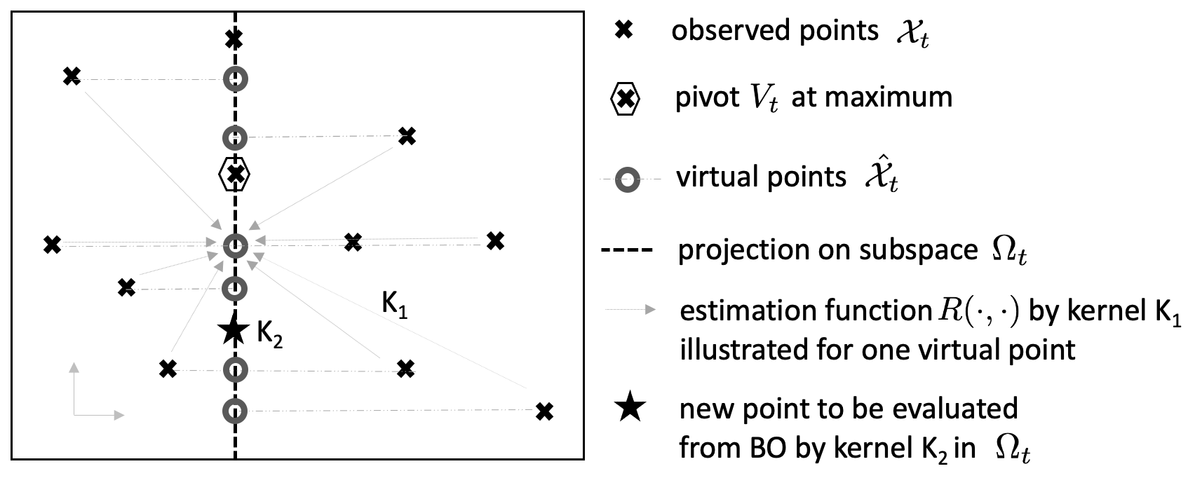
Figure 2: Illustrate of two-stage kernels; stage 1: subspace projection and function value estimation for virtual points using kernel $K_{1}$; stage 2: BO in $\Omega_{t}$ using kernel $K_{2}$

3.1 Block coordinate ascent for subspace selection

We induce a preference distribution $\pi_{t}$ over the coordinate set $I$, and sample a variable-size coordinate block $C_{t}$ accordingly. This distribution is updated at iteration $t$ through a multiplicative weights update method Arora et al. (2012). Specifically, the values of $\pi_{t}$ at coordinates in $C_{t}$ starts off uniform and increase in face of an improvement or decrease otherwise according to different multiplicative ratios $\alpha>1$ and $\beta>1$, respectively,

$$w_{t,j} =w_{t-1,j}\cdot\begin{cases}\alpha&\text{if }j\in C_{t}\text{ and }y_{t}>M_{t-1}\\ 1/\beta&\text{if }j\in C_{t}\text{ and }y_{t}\leq M_{t-1}\\ 1&\text{if }j\notin C_{t}\end{cases}$$ (2)

with $w_{0,j}=\nicefrac{{1}}{{D}}$ and $\pi_{t,j}=\nicefrac{{w_{t,j}}}{{\sum_{j=1}^{D}w_{t,j}}}$. This update characterizes how likely a coordinate block can generate a promising search subspace. The multiplicative ratio $\alpha$ is chosen to be relatively large, e.g., $\alpha=2.0$, and $\beta$ relatively small, e.g., $\beta=1.1$, since the queries that improve the best observations $y_{t}>M_{t-1}$ happen more rarely than the opposite $y_{t}\leq M_{t-1}$.

For selecting the size $|C_{t}|$, we specify an upper bound, e.g. $|C_{t}|\leq 30$, where $|C_{t}|$ can be any random number in a finite set $\mathcal{C}$. Most existing methods partition the coordinates into fixed blocks and select one according to, e.g., cyclic order Wright (June 2015), random sampling or Gauss-Southwell Nutini et al. (July 2015).

3.2 Backoff stopping rule for consistent queries

Observe that only a fraction of the points in $\hat{\mathcal{X}}_{t}\cap\mathcal{X}_{t}$ directly observe the exact function values. The function values on the rest ones in $\hat{\mathcal{X}}_{t}\backslash\mathcal{X}_{t}$ are estimated. For the trade-off between the inaccurate estimations and the exact observations in $\Omega_{t}$, we design a stopping rule that determines the number of consistent queries in $\Omega_{t}$. The more consistent queries conducted in a given subspace, the more accurate observations could be obtained, albeit at the expense of a smaller remaining budget for exploring other regions.

For each iteration $t$, denote the relative improvement at iteration $t$ by

$$\Delta_{t}=\frac{y_{t}-M_{t-1}}{\max(\left|M_{t-1}\right|,0.1)}.$$

When looking backward in time from iteration $t$, we denote by $P_{t}$ the number of consecutive improvements ($\Delta_{s}>0,s\leq t$) and by $N_{t}$ the total number of consecutive queries in the same subspace as in $\Omega_{t}$, respectively. We set

$$C_{t+1} =\begin{cases}\text{a new block},&N_{t}\geq\tau\text{ and }\Delta_{t}\leq 0.1\text{ and }P_{t}\leq\xi\\ C_{t},&N_{t}<\tau\text{ or }\Delta_{t}>0.1\text{ or }P_{t}>\xi\end{cases}$$

where the value $\tau$ depends on the query budget $T$ and the problem dimension $D$, e.g.,

$$\tau=\frac{T}{1000}+\begin{cases}1&D<20\\ 2&20\leq D<70\\ 3&70\leq D<100\\ 4&100\leq D<200\\ 5&200\leq D\end{cases}\qquad\xi=\begin{cases}4&\Delta_{t}<0.05\\ 2&0.05\leq\Delta_{t}\leq 0.1\\ 0&\Delta_{t}>0.1\end{cases}$$

This heuristic stopping rule is designed to take into account several considerations:

1. A maximal query budget ($\tau$) in each subspace grows with the total query budget ($T$) and dimension ($D$).

2. A sufficient progress ($\Delta_{t}$) needs to be made in the subspace to avoid only harvesting marginal improvements due to local fluctuation. The more significant progress the more consecutive improvements ($\xi$) are allowed in this subspace.

This heuristic stopping rule is robust to all the problems presented in this work and to many other that we have tested.

3.3 Theoretical motivation for the subspace selection policy

This section aims at providing some theoretical guidance for specifying the proposed block coordinate selection scheme in section 3.1 rather than it being merely a heuristic. It can be viewed as a combinatorial mixture of experts problem Cesa-Bianchi & Lugosi (2006), where each coordinate is a single expert and the forecaster aims at choosing the best combination of experts in each step. Under this view, we bound the regret of our selection method on an intuitive surrogate loss function with respect to the policy of selecting the best (unknown) block of coordinates at each step. This is complementary to the regret analysis of the optimization procedure performed at each subspace. Specifically, the conventional regret analysis associated with BO, with respect to the value of the objective function, is applicable for each specific subspace, accounting for the projection of points to this subspace. Here we focus on justifying the coordinate selection part alone.

Following the standard framework, we compare with a fixed optimal choice $\mathcal{I}^{*}$ for the block of coordinates to pick at all steps. This block is characterized by improving the objective function for the largest number of times among all the possible coordinate blocks when performing Bayesian optimization. For any coordinate subset $\mathcal{A}$, we define the following loss function at time $t$, for coordinate $i$,

$$\ell_{t,i}(\mathcal{A})=\begin{cases}-\log(\tilde{\alpha})&\text{if }i\in\mathcal{A}\text{ and }y_{t}>M_{t-1}\\ \log(\tilde{\beta})&\text{if }i\in\mathcal{A}\text{ and }y_{t}\leq\lambda_{t}\\ 0&\text{if }i\notin\mathcal{A}\end{cases}$$ (3)

with $\tilde{\alpha},\tilde{\beta}>1$, where both $y_{t}$ and $M_{t-1}$ are fully determined by the previously selected coordinate subset $C_{1},C_{2},\cdots,C_{t-1},C_{t}$. All the coordinates participating in the selected block incur the same loss that effectively rewards these coordinates for improving the objective and penalizes these for failing to improve the objective. All other coordinates that are not selected receive a zero loss and remain untouched.

Note that $\tilde{\alpha}$ and $\tilde{\beta}$ express the extent of reward and penalty, e.g. for $\tilde{\alpha}=\tilde{\beta}=e$ we have losses of $\ell_{t,i}\in\{-1,1,0\}$. Yet, $\tilde{\alpha}$ is chosen to be larger than $\tilde{\beta}$, since the frequency of improving the objective is expected to be smaller.

The loss received by the forecaster is to reflect the same motivation. This is done by averaging the losses of the individual coordinates in the selected block, so that the size of the block does not matter explicitly, i.e. a bigger block should not incur more loss just due to its size but only due to its performance. Such that for each coordinate block $\mathcal{I}_{t}\subset\mathcal{I}=\{1,\cdots,D\}$ selected at time step $t$, the loss incurred by the forecaster is $L_{t,\mathcal{I}_{t}}=\frac{1}{|\mathcal{I}_{t}|}\sum_{i\in\mathcal{I}_{t}}\ell_{t,i}$. This is also the common loss incurred by all the coordinates participating in that block.

In each step we have the following multiplicative update rule of the weights associated with each coordinate

$$w_{t,i} =w_{t-1,i}\cdot e^{-\eta\ell_{t,i}(C_{t};y_{t},M_{t-1})}=w_{t-1,i}\cdot\begin{cases}\tilde{\alpha}^{\eta}&\text{if }i\in C_{t}\text{ and }y_{t}>M_{t-1}\\ 1/\tilde{\beta}^{\eta}&\text{if }i\in C_{t}\text{ and }y_{t}\leq M_{t-1}\\ 1&\text{if }i\notin C_{t},\end{cases}$$ (4)

which, by setting $\alpha=\tilde{\alpha}^{\eta}$ and $\beta=\tilde{\beta}^{\eta}$, yields the update rule in Eq. (2).

The probability $\tilde{\pi}_{t,\mathcal{I}_{t}}$ of selecting a certain coordinate block $\mathcal{I}_{t}$ is induced by $\pi_{t}$ as specified next. Thus the expected cumulative loss of the forecaster is:

$$L_{T}=\sum_{t=1}^{T}\sum_{c\in\mathcal{C}}\sum_{\mathcal{I}_{t}\in\mathcal{S}_{c}}\tilde{\pi}_{t,\mathcal{I}_{t}}\cdot\frac{1}{|\mathcal{I}_{t}|}\sum_{i\in\mathcal{I}_{t}}\ell_{t,i}$$

Assume that the best coordinate block is $\mathcal{I}^{*}$, then the corresponding cumulative loss is:

$$L_{T}^{*} =\sum_{t=1}^{T}L_{t,\mathcal{I}^{*}}=\sum_{t=1}^{T}\frac{1}{|\mathcal{I}^{*}|}\sum_{i\in\mathcal{I}^{*}}\ell_{t,i}$$

We hence aim at bounding the regret $\mathcal{R}_{T}=L_{T}-L_{T}^{*}$.

Theorem 3.1

Sample from the combinatorial space of all possible coordinate blocks $\mathcal{I}_{t}\in\bigcup_{c\in\mathcal{C}}\mathcal{S}_{c}$ with probability $\tilde{\pi}^{c}_{t,\mathcal{I}_{t}}=\nicefrac{{\prod_{i\in\mathcal{I}_{t}}\tilde{w}_{t,\mathcal{I}_{t}}}}{{\sum_{c\in\mathcal{C}}\sum_{\hat{\mathcal{I}}\in\mathcal{S}_{c}}\prod_{j\in\hat{\mathcal{I}}}\tilde{w}_{t,\hat{\mathcal{I}}}}}$. Then the update rule in Eq. (2) with $\alpha=\tilde{\alpha}^{\eta}$, $\beta=\tilde{\beta}^{\eta}$ and $\eta=\log(\tilde{\alpha}\tilde{\beta})^{-1}\sqrt{T^{-1}|\mathcal{C}|D\log(D)}$ yields

$$\mathcal{R}_{T}\leq\mathcal{O}\left(\log(\tilde{\alpha}\tilde{\beta})\cdot\sqrt{T|\mathcal{C}|D\log(D)}\right),$$ (5)

where $\tilde{w}_{t,\mathcal{I}_{t}}=\prod_{i\in\mathcal{I}_{t}}w_{t,i}^{\nicefrac{{1}}{{|\mathcal{I}_{t}|}}}$ is the geometric mean of the weights for block $\mathcal{I}_{t}$.

The upper bound in Eq. (5) is tight, as the lower bound can be shown to be of $\Omega(\sqrt{T\log(N)})$ Haussler et al. (1995) where the number of experts is $N=\sum_{c\in\mathcal{C}}\mathcal{S}_{c}\leq D^{|\mathcal{C}|D}$ in our combinatorial setup, as typically $|\mathcal{C}|\ll D$.

In practice, the direct sampling policy introduced in Theorem 3.1 involves high computational costs due to the exponential growth of combinations in $D$. Thus CobBO suggests an alternative computationally efficient sampling policy with a linear growth in $D$.

Theorem 3.2

Sample a block size $c\in\mathcal{C}$ with probability $p_{c}$ and $c$ coordinates without replacement according to $\pi_{t}$. Assume $\mathcal{C}\supset\{1\}$, then the update rule in Eq. (2), with $\alpha=\tilde{\alpha}^{\eta}$, $\beta=\tilde{\beta}^{\eta}$ and
$\eta=\sqrt{\frac{\log(D)}{T(\log(\tilde{\alpha}\tilde{\beta})^{2}-\log(p_{1}))}}\geq 1$ yields

$$\mathcal{R}_{T}\leq\mathcal{O}\left(\sqrt{(\log(\tilde{\alpha}\tilde{\beta})^{2}-\log(p_{1}))}\cdot\sqrt{T\log(D)})\right),$$ (6)

where $p_{c}>0$ for all $c\in\mathcal{C}$ and $\sum_{c\in\mathcal{C}}p_{c}=1$.

The proof and detailed sampling policy are in appendix A. The regret upper bound in Eq. 6 is tight, as the lower bound for an easier setup can be shown to be of $\Omega(\sqrt{T\log(D)})$ Haussler et al. (1995). The implication on $\eta$ is valid only for settings of a high dimension and low query budget. In particular, CobBO is designed for this kind of problems. Similar analysis and results follow when incorporating consistent queries from section 3.2 and sampling a new coordinate block once every several steps. This is done by effectively performing less steps of aggregated temporal losses, as shown in appendix A.3.

4 Numerical Experiments

This section presents detailed ablation studies of the key components and comparisons with other algorithms. The specifications of the testbed are as follows: Intel(R) Xeon(R) CPU E5-2682 v4 2.50GHz, Memory 32GB, GPU NVIDIA Tesla P100 PCIe 16GB.

4.1 Ablation study and empirical analysis

Ablation studies are designed to study the contributions of the key components in Algorithm 2 by experimenting with the Rastrigin function on $[-5,10]^{50}$ with 20 initial points. Confidence intervals ($95\%$) over $10$ independent experiments for each configuration are presented in Fig. 3,  4 and  5.

The upper bound of the block sizes: At each iteration, the block size $|C_{t}|$ of CobBO is uniformly sampled from a set formed through capping the elements from $\{1,4,6,8,12,14,16,22,24,26,30\}$ by the dimension $D$ of the problem. Hence the average block size is about $15$, the lower bound is $1$ and the upper bound is $30$. This set is chosen to prefer relatively lower dimensions and works well for the problems we experimented with. In Fig. 3 we present an ablation study focusing on the selection of the upper bound of this set, which plots the means and variances of the best searched function values for Rastrigin on $[-3,4]^{50}$. Considering that the differences of the mean values of the best obtained minimization solutions are small compared to the standard deviations, we conclude that the algorithm is not very sensitive to the choice of the upper bound, while higher values are slightly favourable, as expected, yet require more computation.

Figure 3: Impact of the block size upper bound on the best function values for Rastrigin on $[-3,4]^{50}$

Coordinate blocks of a varying size: CobBO selects a block of coordinates $C_{t}$ of a varying size, as described in Section 3.1. The above ablation study in Fig. 3 shows that CobBO is quite robust to the upper bound of the block size $|C_{t}|$. Fig. 4 (left) shows that a varying size is better than a fixed one. Furthermore, although the average block size of CobBO is $15$ in this setting, it enjoys both the fast exploration of larger block sizes (e.g. $22$) and efficient exploitation of smaller block sizes (e.g. $6$).

RBF interpolation in the first stage: RBF calculation is time efficient, which is very beneficial in high dimensions. Fig. 1 (left) shows the computation time of plain Bayesian optimization compared to CobBO’s. While the former applies GP regression using the Matérn kernel in the high dimensional space directly, the later applies RBF interpolation in the high dimensional space and GP regression with the Matérn kernel in the low dimensional subspace. This two-stage kernel method leads to a significant speed-up. Other time efficient alternatives are, e.g., the inverse distance weighting Shepard (1968) and the simple approach of assigning the value of the observed nearest neighbour. Fig. 4 (middle) shows that RBF is more favorable.

Backoff stopping rule: CobBO applies a stopping rule to query a variable number of points in subspace $\Omega_{t}$ (Section 3.2). To validate its effectiveness, we compare it with schemes that use a fixed budget of queries for $\Omega_{t}$. Fig. 4 (right) shows that the stopping rule yields superior results. Specifically, it enjoys both fast exploration of small query budget in each subspace (e.g. $1$,$2$) and efficient exploitation of large ones (e.g. $16$). Note that for different problems the best fixed number of consistent queries vary but the backoff stopping rule can adaptively achieve a good performance.

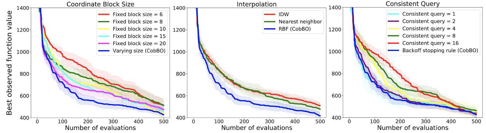
Figure 4: Ablation study using Rastrigin on $[-5,10]^{50}$ with $20$ initial random samples

Figure 5: The preference probability focuses on active coordinates

Preference probability over coordinates: For demonstrating the effectiveness of coordinate selection (Section 3.1), we artificially let the function value only depend on the first $25$ coordinates of its input and ignore the rest. It forms two separate sets of active and inactive coordinates, respectively. We expect CobBO to refrain from selecting inactive coordinates. Fig. 5 shows the overall preference probability $\pi_{t}$ for picking active ($\sum_{i=1}^{25}\pi_{t,i}$) and inactive coordinates ($\sum_{i=26}^{50}\pi_{t,i}$) at each iteration $t$. We see that the preference distribution concentrates on the active coordinates.

4.2 Comparisons with other methods

We fix a default configuration for CobBO identically across all of the experiments. Extensive experiments show that CobBO performs on par or outperforms a collection of state-of-the-art methods. Most of the experiments are conducted using the same settings as in TurBO Eriksson et al. (2019), where it is compared with a comprehensive list of baselines, including BFGS, BOCK Oh et al. (2018), BOHAMIANN, CMA-ES Hansen & Ostermeier (2001), BOBYQA, EBO Wang et al. (2018), GP-TS, HeSBO Munteanu et al. (2019), Nelder-Mead and random search. To avoid repetitions, we only show TuRBO and CMA-ES that achieve the best performance among this list, and additionally compare with BADS Acerbi & Ma (2017), Tree Parzen Estimator (TPE) Bergstra et al. (2011) and Adaptive TPE (ATPE) ElectricBrain (2018). Since CobBO is designed for high dimensional problems, we benchmark the performance in Section 4.2.1 in high dimensions. To show that it also works in low dimensions, we conduct the low dimensional tests in Section 4.2.2. As mentioned in Section 2, the embedding algorithms (e.g., REMBO Wang et al. (2016) and ALEBO Letham et al. (2020)) and CobBO are based on different assumptions, which are compared in Section 4.2.3. Section 4.2.4 presents the comparison with LineBO Kirschner et al. (2019).

4.2.1 High dimensional tests

Since the duration of each experiment in this section is long, confidence intervals ($95\%$) over repeated 10 independent experiments for each problem are shown.

Figure 6: Performance over high dimensional synthetic problems: Levy (left) and Rastrigin (right)

The 100 dimensional synthetic black-box functions (minimization): We minimize the Levy and Rastrigin functions on $[-5,10]^{100}$ with $300$ initial points. These two problems are challenging since they have no redundant dimensions. TuRBO is configured with $1$ trust regions and a batch size of $100$. Fig. 6 (left) shows that CobBO can greatly reduce the trial complexity. For Levy and Rastrigin, CobBO surpasses the final solutions of all the other methods within $2,000$ and $5,000$ trials for a total budget of $10,000$ trials, respectively. REMBO is especially compared in Section 4.2.3.

In order to highlight the difference of the running time, we test Ackley 200D with $10,000$ trials. For a fair comparison, we change the configure so that both TurBO and CobBO have the same batch size of $1$. CobBO runs for $12.8$ CPU hours and TuRBO-1 runs for more than $80$ CPU hours or $9.6$ GPU hours. Other methods either take too long to make progress or find far worse solutions.

Additive latent structure (minimization): As mentioned in Section 2, additive latent structures have been explored for tackling challenges in high dimensions. We construct two additive functions. The first one has 36 dimensions, defined as $f_{36}(x)=\rm{Ackley}(x_{1})+\rm{Levy}(x_{2})+\rm{Rastrigin}(x_{3})+\rm{Hartmann}(x_{4})$, where the first three terms express the exact functions and domains described in Section 4.2.2, with the Hartmann function defiend over $[0,1]^{6}$. The second has 56 dimensions, defined as $f_{56}(x)=\rm{Ackley}(x_{1})+\rm{Levy}(x_{2})+\rm{Rastrigin}(x_{3})+\rm{Hartmann}(x_{4})+\rm{Rosenbrock}(x_{5})+\rm{Schwefel}(x_{6})$, where the first four terms are the same as those of $f_{36}$, with the Rosenbrock and Schwefel functions defined over $[-5,10]^{10}$ and $[-500,500]^{10}$, respectively.

We compare CobBO with TPE, ATPE, BADS, CMA-ES and TuRBO, each with $100$ initial points. Specifically, TuRBO is configured with 15 trust regions and a batch size 50 for $f_{36}$ and $100$ for $f_{56}$. ATPE is excluded for $f_{56}$ as it takes more than 24 hours per run to finish. The results are shown in Fig. 7, where CobBO quickly finds the best solutions for both $f_{36}$ and $f_{56}$.

As shown in Fig. 7, CobBO finds the best solutions for both $f_{36}$ and $f_{56}$. BADS performs closely to CobBO. ATPE outperforms TPE, TuRBO and CMA-ES on $f_{36}$. TuRBO surpasses TPE and CMA-ES on $f_{36}$ eventually, while TPE and CMA-ES converge faster than TuRBO on $f_{56}$.

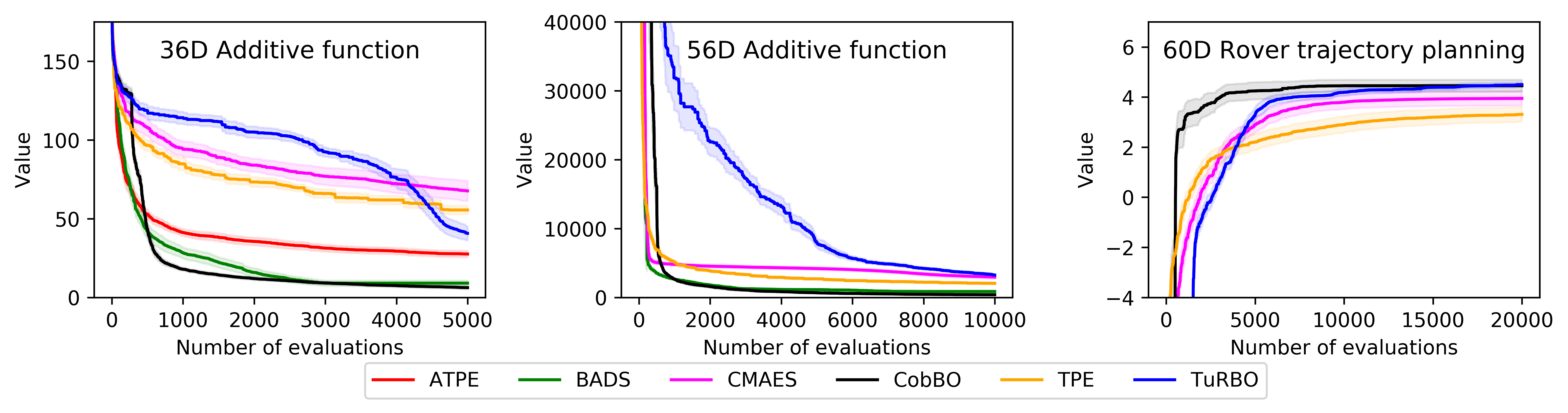
Figure 7: Performance over medium-size dimensional problems: 36D (left) and 56D (middle) additive functions and the 60D rover trajectory planning (right)

Rover trajectory planning (maximization): This problem (60 dimensions) is introduced in Wang et al. (2018). The objective is to find a collision-avoiding trajectory of a sequence consisting of 30 positions in a 2-D plane. We compare CobBO with TuRBO, TPE and CMA-ES with a budget of $20,000$ evaluations and $200$ initial points. TuRBO is configured with $15$ trust regions and a batch size of $100$, as in Eriksson et al. (2019). ATPE, BADS and REMBO are excluded for this problem and the following ones, as they all last for more than 24 hours per run. The result is shown in Fig. 7. CobBO reaches the best solution with fewer evaluations than TuRBO, while TPE and CMA-ES reach inferior solutions.

4.2.2 Low dimensional tests

To evaluate the performance of CobBO on low dimensional problems, we use two more challenging problems of lunar landing Eriksson et al. (2019) and robot pushing Wang et al. (2018), as well as classic synthetic black-box functions Surjanovic & Bingham (2013), by following the setup in Eriksson et al. (2019) for most of the experiments. Confidence intervals ($95\%$) over repeated 30 independent experiments for each problem are shown.

Lunar landing (maximization): This controller learning problem ($12$ dimensions) is provided by the OpenAI gym and evaluated in Eriksson et al. (2019). Each algorithm has 50 initial points and a budget of $1,500$ trials. TuRBO is configured with 5 trust regions and a batch size of 50 as in Eriksson et al. (2019). Fig. 8 shows that, among the $30$ independent tests, CobBO quickly exceeds $300$ along some good sample paths, outperforming other algorithms.

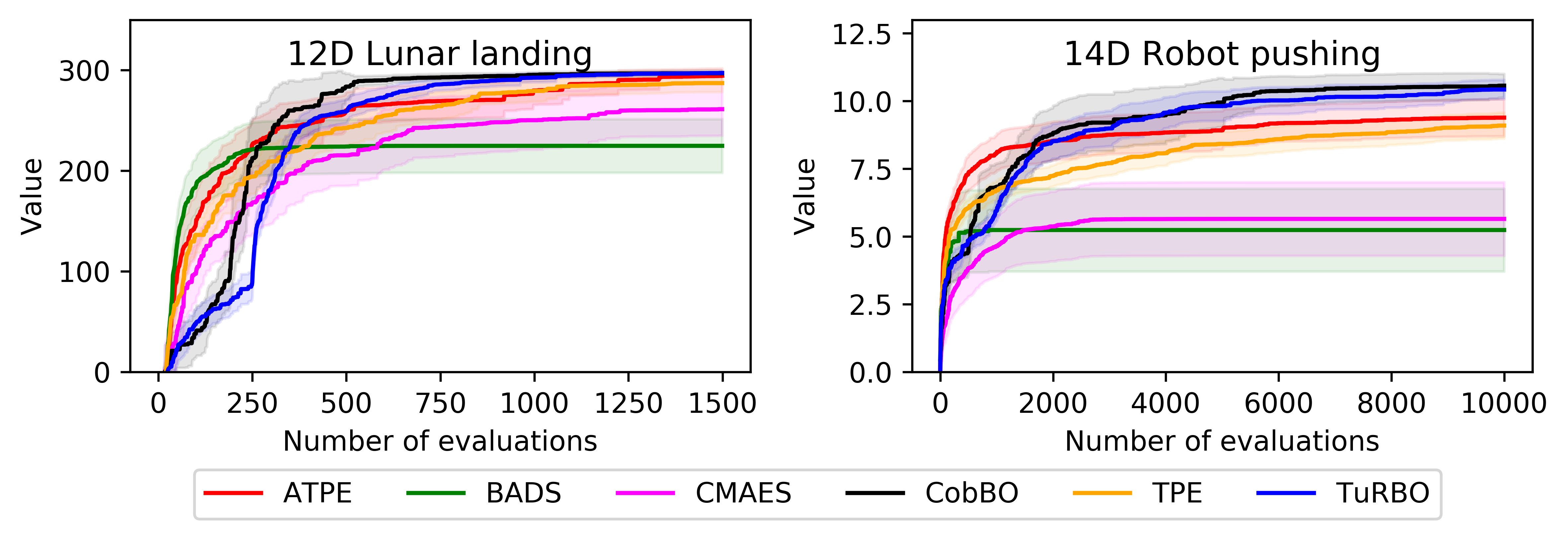
Figure 8: Performance over the lunar landing (left) and robot pushing (right) problems

Robot pushing (maximization): This control problem (14 dimensions) is introduced in Wang et al. (2018) and extensively tested in Eriksson et al. (2019). We follow the setting in Eriksson et al. (2019), where TuRBO is configured with a batch size of 50 and 15 trust regions where each has 30 initial points. We exclude REMBO that takes too long per run (more than $24$ hours). Each experiment has a budget of $10,000$ evaluations. On average CobBO exceeds 10.0 within 5,500 trials, while TuRBO requires about 7,000, as shown in Fig.  8. TPE and ATPE converge to around 9.0, outperforming BADS and CEM-ES with large margins. The latter two exhibit large variations and get stuck at local optima.

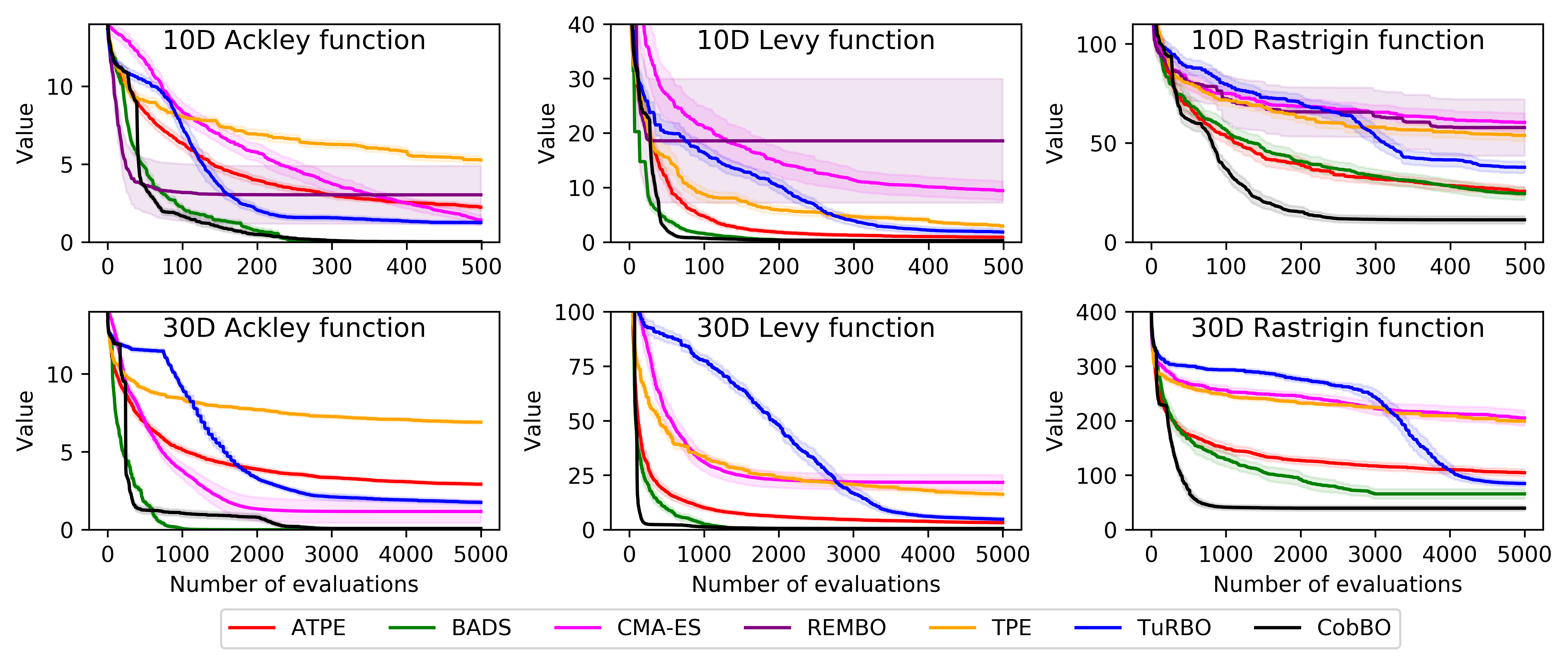
Figure 9: Performance on 10D (top) and 30D (bottom) synthetic black-box functions: Ackley (left), Levy (middle) and Rastrigin (right)

Classic synthetic black-box functions (minimization): Three popular synthetic functions ($10$ and $30$ dimensions) are chosen, including Ackley over $[-5,10]^{10}$ and $[-5,10]^{30}$, Levy over both $[-5,10]^{10}$ and $[-5,10]^{30}$, and Rastrigin over both $[-3,4]^{10}$ and $[-3,4]^{30}$. TuRBO is configured identically the same as in Eriksson et al. (2019), with a batch size of $10$ and $5$ concurrent trust regions where each has $10$ initial points. The other algorithms use $20$ initial points. The results are shown in Fig. 9. CobBO shows competitive or better performance for all of these problems. It finds the global optima on Ackley and Levy, and clearly outperforms the other algorithms for the difficult Rastrigin function. Notably, BADS is more suitable for low dimensions, as commented in Acerbi & Ma (2017), which performs close to CobBO except on Rastrigin. TuRBO performs better than TPE and worse than BADS. ATPE outperforms TPE. CMA-ES eventually catches up with TPE, ATPE and REMBO on Ackley. For $10$ dimensions, REMBO appears unstable with large variations and is trapped at local optima. For $30$ dimensions, REMBO is excluded as it takes too long to finish; see Section 4.2.3.

4.2.3 Comparison to REMBO and ALEBO

REMBO Wang et al. (2016) and ALEBO Letham et al. (2020) are designed for high-dimensional (large $D$) problems with low intrinsic dimensions (small $d$), which essentially assumes that the function does not change along certain directions. They do not necessarily perform well for problems without redundant dimensions, as shown by the following experiments with $D=d$.

First, we compare REMBO and CobBO using Ackley 200D with $4000$ iterations and $50$ initial points. Even though $D=d=200$ in this case, we treat REMBO as if the effective dimension were $d=20$, similar to CobBO’s subspaces with an average size about $15$. REMBO and CobBO reach the mean best values of $15.1$ and $3.8$, respectively, running for $31.2$ and $3.4$ hours, respectively. This shows that CobBO could outperform REMBO by a large margin for problems without redundant dimensions. In addition, CobBO requires about $10\%$ of the computation time of REMBO for this experiment, which demonstrates the advantage of the two-stage kernels in reducing the computation time.

Next, we compare with ALEBO, which has demonstrated great performance for problems with large $D$ but small $d$ in Letham et al. (2020). Through extensive experiments we find that ALEBO works only when the underlying effective dimension satisfies $d\leq 20$. Otherwise, the algorithm suffers from the same curse of dimensionality as vanilla BO algorithms do, since the subproblem in the embedding space of $d$ dimensions is also challenging for large $d$.

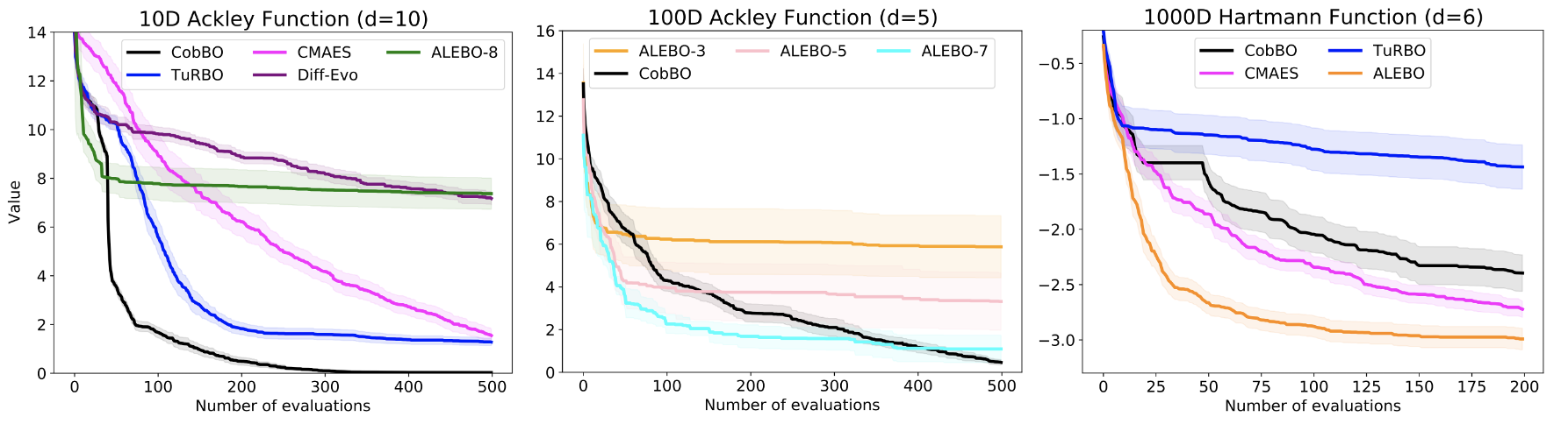
Figure 10: Experiments with $D=10,100,1000$ spaces of small effective dimensions $d=10,5,6$, respectively

To this end, we design three different experiments. First, we study the general problems for $D=d$. Since ALEBO has performance issues for large $d$, we test Ackley ($D=d=10$). As ALEBO requires $d<D$, we treat it as if $d=8$ (ALEBO-8). In this case, ALEBO does not show good performance and is outperformed by CobBO, TurBO and CMAES, as shown in Fig. 10 (left). Second, we test Ackley ($D=100,d=5$). In reality, we do not know the effective dimension $d$. Therefore, we teat it as if $d=3,5,7$ to obtain ALEBO-3, ALEBO-5 and ALEBO-7, respectively. Although this problem indeed has a very small $d=5$, CobBO can still perform well compared to ALEBO, as shown in Fig. 10 (middle). The third experiment is using exactly the same setting as in Letham et al. (2020) for Hartmann6 with $D=1000$ and $d=6$. As shown in Fig. 10 (right), ALEBO outperforms CobBO, since CobBO is not designed for a function with a very high dimension $D=1000$ and a very low effective dimension $d=6$. The reason is because CobBO relies on selection of subspaces of an average dimension $15$, which cannot easily cover the optima in a high dimensional space $D\geq 1000$. In this case, after projecting the original function into a low $d$ dimensional embedding space, CobBO can be applied to solve the subproblem when $d$ is still considered to be too large, e.g., $d>20$.

4.2.4 Comparison to LineBO

Although sharing some common basic ideas, LineBO Kirschner et al. (2019) reduces the acquisition maximization cost by restricting on a line, but it does not address the computational issue of the GP regression in the full space by using a single kernel, i.e., the first stage of CobBO. In addition, it is difficult to find a good direction to form the line space at each iteration, since searching for the optima in a high dimensional space on a random line is not computationally efficient. Fig. 11 shows that LineBO is significantly outperformed by CobBO using a typical example, e.g., Ackley, with $D=10,30$.

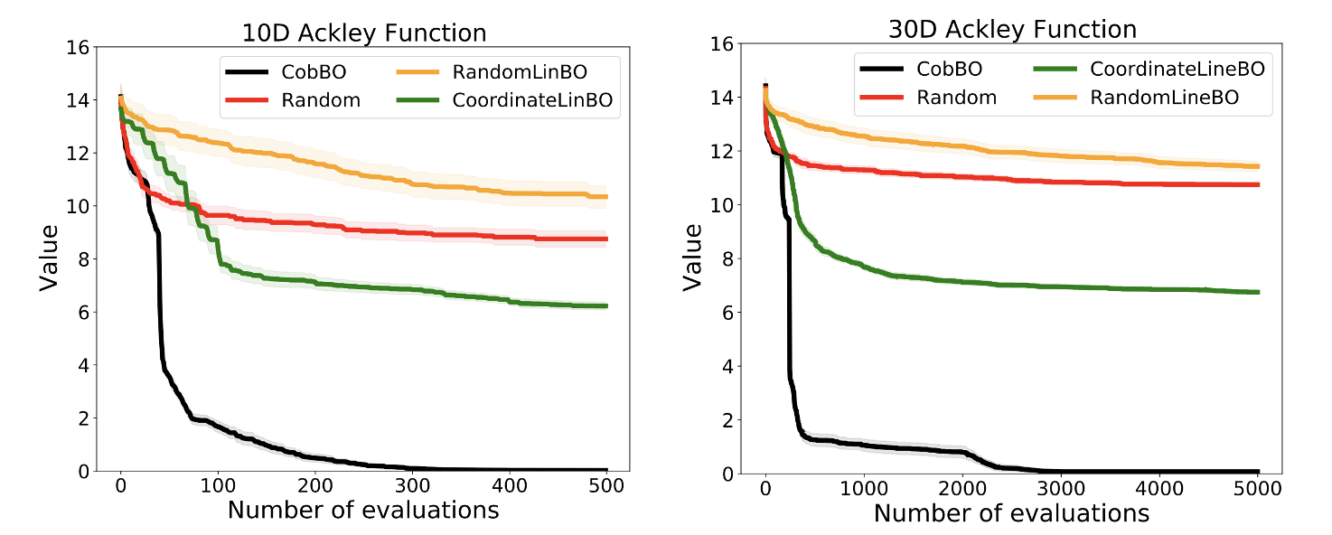
Figure 11: CobBO outperforming different variants of LineBO

For $D=10$ with a query budget of $500$, CobBO almost reaches the optimal solution $0.0$ while LineBO (CoordinateLineBO) only obtains 6.2. For $D=30$ with a query budget of $5000$, CobBO reaches $0.12$ and LineBO (CoordinateLineBO) only obtains $7.6$. In both cases, RandomLineBO performs even worse than random search.

5 Conclusion

CobBO is a variant of coordinate ascent tailored for Bayesian optimization with a stopping rule to switch coordinate subspaces. The sampling policy of subspaces is proven to have tight regret bounds with respect to the best subspace in hindsight. Combining the projection on random subspaces with a two-stage kernels for function value interpolation and GP regression, we provide a practical Bayesian optimization method of affordable computational costs in high dimensions. Empirically, CobBO consistently finds comparable or better solutions with reduced trial complexity in comparison with the state-of-the-art methods across a variety of benchmarks.

Supplementary Material

Appendix A Proofs

In this section we provide proofs for the theorems in Section 3.3. To make non-negative temporal losses, we modify the losses in Eq. (3) to be non-negative by adding the same constant $\log(\tilde{\alpha})$,

$$\tilde{\ell}_{t,i}=\begin{cases}0&\text{if }i\in C_{t}\text{ and }y_{t}>M_{t-1}\\ \log(\tilde{\alpha}\tilde{\beta})&\text{if }i\in C_{t}\text{ and }y_{t}\leq M_{t-1}\\ \log(\tilde{\alpha})&\text{if }i\notin C_{t}.\end{cases}$$

This modification does not change the resulted distribution $\pi_{t}$ induced over the coordinates as it is invariant to shifts of the losses, $\pi_{t,i}=w_{t,i}/W_{t}$,

$$\pi_{t,i}=\frac{e^{-\eta\sum_{\tau=1}^{t}\tilde{\ell}_{\tau,i}}}{\sum_{j=1}^{D}e^{-\eta\sum_{\tau=1}^{t}\tilde{\ell}_{\tau,j}}} =\frac{e^{-\eta\sum_{\tau=1}^{t}(\ell_{\tau,i}+\log(\tilde{\alpha}))}}{\sum_{j=1}^{D}e^{-\eta\sum_{\tau=1}^{t}(\ell_{\tau,j}+\log(\tilde{\alpha}))}}$$

$$=\frac{e^{-\eta t\log(\tilde{\alpha})}e^{-\eta\sum_{\tau=1}^{t}\ell_{\tau,i}}}{e^{-\eta t\log(\tilde{\alpha})}\sum_{j=1}^{D}e^{-\eta\sum_{\tau=1}^{t}\ell_{\tau,j}}}=\frac{e^{-\eta\sum_{\tau=1}^{t}\ell_{\tau,i}}}{\sum_{j=1}^{D}e^{-\eta\sum_{\tau=1}^{t}\ell_{\tau,j}}}.$$

Thus, $\tilde{\pi}_{t,i}$ and $\hat{\pi}_{t,i}$ introduced in Sections A.1 and  A.2 remain unchanged as well. For simplicity we refer to $\tilde{\ell}$ as $\ell$ throughout this section.

A.1 Regret analysis for sampling from the combinatorial space of coordinate blocks

The probability $\tilde{\pi}_{t,\mathcal{I}_{t}}$ of selecting a certain coordinate block $\mathcal{I}_{t}\subset\mathcal{I}=\{1,\cdots,D\}$ of size $|\mathcal{I}_{t}|=c\in\mathcal{C}$ follows sampling according to $\pi_{t}$ such that

$$\tilde{w}_{t,\mathcal{I}_{t}}=\prod_{i\in\mathcal{I}_{t}}w_{t,i}^{\frac{1}{|\mathcal{I}_{t}|}}\;,\quad\tilde{W}_{t}=\sum_{c\in\mathcal{C}}\sum_{\mathcal{I}_{t}\in\mathcal{S}_{c}}\tilde{w}_{t,\mathcal{I}_{t}}\;,\quad\tilde{\pi}_{t,\mathcal{I}_{t}}=\frac{\tilde{w}_{t,\mathcal{I}_{t}}}{\tilde{W}_{t}}\quad\forall\mathcal{I}_{t}\in\bigcup_{c\in\mathcal{C}}\mathcal{S}_{c}$$ (7)

with

$$\sum_{c\in\mathcal{C}}\sum_{\mathcal{I}_{t}\in\mathcal{S}_{c}}\tilde{\pi}_{t,\mathcal{I}_{t}}=1.$$ (8)

Lemma A.1

For $\eta>0$ and non-negative losses $\ell_{t,i}\geq 0$ the update rule in (4) satisfies for any block of coordinates $\mathcal{I}^{*}$:

$$\sum_{t=1}^{T}\sum_{c\in\mathcal{C}}\sum_{\mathcal{I}_{t}\in\mathcal{S}_{c}} \tilde{\pi}_{t,\mathcal{I}_{t}}\cdot\frac{1}{|\mathcal{I}_{t}|}\sum_{i\in\mathcal{I}_{t}}\ell_{t,i}-\sum_{t=1}^{T}\frac{1}{|\mathcal{I}^{*}|}\sum_{i\in\mathcal{I}^{*}}\ell_{t,i}\leq$$

$$\eta\sum_{t=1}^{T}\sum_{c\in\mathcal{C}}\sum_{\mathcal{I}_{t}\in\mathcal{S}_{c}}\tilde{\pi}_{t,\mathcal{I}_{t}}\cdot\left(\frac{1}{|\mathcal{I}_{t}|}\sum_{i\in\mathcal{I}_{t}}\ell_{t,i}\right)^{2}+\frac{D\log(D)}{\eta}.$$ (9)

Proof: Set

$$\tilde{w}_{0,\mathcal{I}_{t}}=1\quad\forall\mathcal{I}_{t}\in\bigcup_{c\in\mathcal{C}}\mathcal{S}_{c}$$ (10)

Thus,

$$\tilde{W}_{t+1} =\sum_{c\in\mathcal{C}}\sum_{\mathcal{I}_{t}\in\mathcal{S}_{c}}\tilde{w}_{t+1,\mathcal{I}_{t}}=\sum_{c\in\mathcal{C}}\sum_{\mathcal{I}_{t}\in\mathcal{S}_{c}}\prod_{i\in\mathcal{I}_{t}}w_{t+1,i}^{\frac{1}{|\mathcal{I}_{t}|}}$$

$$=\sum_{c\in\mathcal{C}}\sum_{\mathcal{I}_{t}\in\mathcal{S}_{c}}\prod_{i\in\mathcal{I}_{t}}w_{t,i}^{\frac{1}{|\mathcal{I}_{t}|}}e^{-\frac{\eta}{|\mathcal{I}_{t}|}\ell_{t,i}}=\sum_{c\in\mathcal{C}}\sum_{\mathcal{I}_{t}\in\mathcal{S}_{c}}\prod_{i\in\mathcal{I}_{t}}w_{t,i}^{\frac{1}{|\mathcal{I}_{t}|}}\cdot e^{-\frac{\eta}{|\mathcal{I}_{t}|}\sum_{i\in\mathcal{I}_{t}}\ell_{t,i}}$$

$$=\sum_{c\in\mathcal{C}}\sum_{\mathcal{I}_{t}\in\mathcal{S}_{c}}\tilde{w}_{t,\mathcal{I}_{t}}\cdot e^{-\frac{\eta}{|\mathcal{I}_{t}|}\sum_{i\in\mathcal{I}_{t}}\ell_{t,i}}$$

$$=\tilde{W}_{t}\sum_{c\in\mathcal{C}}\sum_{\mathcal{I}_{t}\in\mathcal{S}_{c}}\tilde{\pi}_{t,\mathcal{I}_{t}}\cdot e^{-\frac{\eta}{|\mathcal{I}_{t}|}\sum_{i\in\mathcal{I}_{t}}\ell_{t,i}}$$ (11)

$$\leq\tilde{W}_{t}\sum_{c\in\mathcal{C}}\sum_{\mathcal{I}_{t}\in\mathcal{S}_{c}}\tilde{\pi}_{t,\mathcal{I}_{t}}\left(1-\frac{\eta}{|\mathcal{I}_{t}|}\sum_{i\in\mathcal{I}_{t}}\ell_{t,i}+\eta^{2}\left(\frac{1}{|\mathcal{I}_{t}|}\sum_{i\in\mathcal{I}_{t}}\ell_{t,i}\right)^{2}\right)$$ (12)

$$\leq\tilde{W}_{t}\left(1+\sum_{c\in\mathcal{C}}\left(\sum_{\mathcal{I}_{t}\in\mathcal{S}_{c}}\eta^{2}\tilde{\pi}_{t,\mathcal{I}_{t}}\left(\frac{1}{|\mathcal{I}_{t}|}\sum_{i\in\mathcal{I}_{t}}\ell_{t,i}\right)^{2}-\frac{\eta}{|\mathcal{I}_{t}|}\tilde{\pi}_{t,\mathcal{I}_{t}}\sum_{i\in\mathcal{I}_{t}}\ell_{t,i}\right)\right)$$ (13)

$$\leq\tilde{W}_{t}e^{\sum_{c\in\mathcal{C}}\cdot\left(\sum_{\mathcal{I}_{t}\in\mathcal{S}_{c}}\eta^{2}\tilde{\pi}_{t,\mathcal{I}_{t}}\left(\frac{1}{|\mathcal{I}_{t}|}\sum_{i\in\mathcal{I}_{t}}\ell_{t,i}\right)^{2}-\frac{\eta}{|\mathcal{I}_{t}|}\tilde{\pi}_{t,\mathcal{I}_{t}}\sum_{i\in\mathcal{I}_{t}}\ell_{t,i}\right),}$$ (14)

where (11) follows from (7), (12) holds since $e^{-x}\leq 1-x+x^{2}$ for $x\geq 0$, (13) holds due to Eq. (8) and (14) holds since $1+x\leq e^{x}$.

Due to Eq. (10), we have,

$$\tilde{w}_{t,\mathcal{I}_{t}}=\prod_{i\in\mathcal{I}_{t}}w_{t,i}^{\frac{1}{|\mathcal{I}_{t}|}}=\prod_{i\in\mathcal{I}_{t}}w_{0,i}^{\frac{1}{|\mathcal{I}_{t}|}}e^{-\frac{\eta}{|\mathcal{I}_{t}|}\sum_{t=1}^{T}\ell_{t,i}}=e^{-\frac{\eta}{\mathcal{I}_{t}}\sum_{t=1}^{T}\sum_{i\in\mathcal{I}_{t}}\ell_{t,i}}.$$ (15)

And,

$$W_{0}=\sum_{c\in\mathcal{C}}\sum_{\mathcal{I}_{t}\in\mathcal{S}_{c}}\tilde{w}_{0,\mathcal{I}_{t}}=\sum_{c\in\mathcal{C}}\sum_{\mathcal{I}_{t}\in\mathcal{S}_{c}}1=\sum_{c\in\mathcal{C}}|\mathcal{S}_{c}|=\sum_{c\in\mathcal{C}}{D\choose c}\leq(D!)^{|\mathcal{C}|}.$$ (16)

Given that the weight of a certain coordinate block $\mathcal{I}^{*}$ is less than the total sum of all weights, together with Eq. (14), (10) and (16) we have

$$e^{-\frac{\eta}{|\mathcal{I}^{*}|}\sum_{t=1}^{T}\sum_{i\in\mathcal{I}^{*}}\ell_{t,i}} =\tilde{w}_{t,\mathcal{I}^{*}}\leq\tilde{W}_{T}$$

$$\leq(D!)^{|\mathcal{C}|}e^{\sum_{t=1}^{T}\sum_{c\in\mathcal{C}}\cdot\left(\sum_{\mathcal{I}_{t}\in\mathcal{S}_{c}}\eta^{2}\tilde{\pi}_{t,\mathcal{I}_{t}}\left(\frac{1}{|\mathcal{I}_{t}|}\sum_{i\in\mathcal{I}_{t}}\ell_{t,i}\right)^{2}-\frac{\eta}{|\mathcal{I}_{t}|}\tilde{\pi}_{t,\mathcal{I}_{t}}\sum_{i\in\mathcal{I}_{t}}\ell_{t,i}\right)}.$$

Taking the $\log$ of both sides, we have

$$-\eta\sum_{t=1}^{T}\frac{1}{|\mathcal{I}^{*}|}\sum_{i\in\mathcal{I}^{*}}\ell_{t,i}\leq \sum_{t=1}^{T}\sum_{c\in\mathcal{C}}\cdot\left(\sum_{\mathcal{I}_{t}\in\mathcal{S}_{c}}\eta^{2}\tilde{\pi}_{t,\mathcal{I}_{t}}\left(\frac{1}{|\mathcal{I}_{t}|}\sum_{i\in\mathcal{I}_{t}}\ell_{t,i}\right)^{2}-\frac{\eta}{|\mathcal{I}_{t}|}\tilde{\pi}_{t,\mathcal{I}_{t}}\sum_{i\in\mathcal{I}_{t}}\ell_{t,i}\right)+|\mathcal{C}|\log(D!),$$

which, using $D!\leq D^{D}$, finishes the proof.

Proof of Theorem 3.1: Since $\ell_{t,i}\leq\log(\tilde{\alpha}\tilde{\beta})$, then

$$\left(\frac{1}{|\mathcal{I}_{t}|}\sum_{i\in\mathcal{I}_{t}}\ell_{t,i}\right)^{2}\leq\left(\frac{1}{|\mathcal{I}_{t}|}\sum_{i\in\mathcal{I}_{t}}\log(\tilde{\alpha}\tilde{\beta})\right)^{2}\leq\log(\tilde{\alpha}\tilde{\beta})^{2}.$$

Thus, due to Eq. (8), one has

$$\sum_{c\in\mathcal{C}}\sum_{\mathcal{I}_{t}\in\mathcal{S}_{c}}\tilde{\pi}_{t,\mathcal{I}_{t}}\cdot\left(\frac{1}{|\mathcal{I}_{t}|}\sum_{i\in\mathcal{I}_{t}}\ell_{t,i}\right)^{2}\leq\sum_{c\in\mathcal{C}}\sum_{\mathcal{I}_{t}\in\mathcal{S}_{c}}\tilde{\pi}_{t,\mathcal{I}_{t}}\log(\tilde{\alpha}\tilde{\beta})^{2}=\log(\tilde{\alpha}\tilde{\beta})^{2}.$$

Setting $\eta=\frac{1}{\log(\tilde{\alpha}\tilde{\beta})}\sqrt{\frac{|\mathcal{C}|D\log(D)}{T}}$ in Eq. (A.1) yields

$$Regret_{t}\leq\eta T\log(\tilde{\alpha}\tilde{\beta})^{2}+\frac{|\mathcal{C}|D\log(D)}{\eta}=2\log(\tilde{\alpha}\tilde{\beta})\sqrt{T|\mathcal{C}|D\log(D)}.$$ (17)

A.2 Regret analysis for sampling coordinates without replacement

Denote by $p_{c}$ the probability of choosing a certain block size $c\in\mathcal{C}$, such that $p_{c}>0$ and $\sum_{c\in\mathcal{C}}p_{c}=1$, e.g., for a uniform sampling of the block size $p_{c}=1/|\mathcal{C}|$ for all $c\in\mathcal{C}$.

The probability $\hat{\pi}_{t,\mathcal{I}_{t}}$ of selecting a certain coordinate block $\mathcal{I}_{t}\subset\mathcal{I}=\{1,\cdots,D\}$ of size $|\mathcal{I}_{t}|=c\in\mathcal{C}$ follows sampling according to $\pi_{t}$ (Eq. (2)) without replacement, such that,

$$\hat{\pi}_{t,\mathcal{I}_{t}} =\sum_{p\in perm(\mathcal{I}_{t})}\prod_{k\in p}{\frac{\pi_{t,k}}{1-\sum_{j\in p_{1:k}}\pi_{t,j}}}$$

$$=\left(\prod_{i\in\mathcal{I}_{t}}\pi_{t,i}\right)\cdot\left(\sum_{p\in perm(\mathcal{I}_{t})}\prod_{k\in p}\left(1-\sum_{j\in p_{1:k}}\pi_{t,j}\right)^{-1}\right)=\mathcal{P}(\mathcal{I}_{t})\cdot\mathcal{R}(\mathcal{I}_{t})$$ (18)

where $perm(\mathcal{I}_{t})$ are all the permutations of the set $\mathcal{I}_{t}$ and $p_{1:k}$ are the first $k$ coordinates in the permutation $p$. Eq. (18) holds due to the common numerator of all permutations where the left term $\mathcal{P}(\mathcal{I}_{t})$ corresponds to the probability of sampling a subset of coordinates with replacement, and the right term $\mathcal{R}(\mathcal{I}_{t})$ is associated with sampling without replacement. Of course, summing over all the possible blocks of size $c$ results $\sum_{\mathcal{I}_{t}\in\mathcal{S}_{c}}\hat{\pi}_{t,\mathcal{I}_{t}}=1$ for all $c\in\mathcal{C}$.

Thus $\tilde{\pi}_{t,\mathcal{I}_{t}}=p_{c}\cdot\hat{\pi}_{t,\mathcal{I}_{t}}$ and the probability of sampling every block of coordinates of any size sum up to $1$ as well:

$$\sum_{c\in\mathcal{C}}\sum_{\mathcal{I}_{t}\in\mathcal{S}_{c}}\tilde{\pi}_{t,\mathcal{I}_{t}}=\sum_{c\in\mathcal{C}}p_{c}\sum_{\mathcal{I}_{t}\in\mathcal{S}_{c}}\hat{\pi}_{t,\mathcal{I}_{t}}=\sum_{c\in\mathcal{C}}p_{c}=1$$ (19)

Lemma A.2

Sample a block size $c\in\mathcal{C}$ with probability $p_{c}>0$ and $c$ coordinates without replacement according to $\pi_{t}$. Assume $\mathcal{C}\supset\{1\}$, $\eta>0$ and non-negative losses $\ell_{t,i}\geq 0$. Then the update rule in (4) satisfies for any block of coordinates $\mathcal{I}^{*}$:

$$\sum_{t=1}^{T}\sum_{c\in\mathcal{C}}p_{c}\sum_{\mathcal{I}_{t}\in\mathcal{S}_{c}}\hat{\pi}_{t,\mathcal{I}_{t}}\cdot \frac{1}{|\mathcal{I}_{t}|}\sum_{i\in\mathcal{I}_{t}}\ell_{t,i}-\sum_{t=1}^{T}\frac{1}{|\mathcal{I}^{*}|}\sum_{i\in\mathcal{I}^{*}}\ell_{t,i}$$

$$\leq\eta\sum_{t=1}^{T}\sum_{c\in\mathcal{C}}p_{c}\sum_{\mathcal{I}_{t}\in\mathcal{S}_{c}}\hat{\pi}_{t,\mathcal{I}_{t}}\cdot\left(\frac{1}{|\mathcal{I}_{t}|}\sum_{i\in\mathcal{I}_{t}}\ell_{t,i}\right)^{2}+\frac{\log(D)}{\eta}-\frac{T\log(p_{1})}{\eta}$$ (20)

Proof: Starting with a uniform distribution over the coordinates $w_{0,i}\equiv\frac{1}{D}$ such that $W_{0}=1$ and we have:

$$p_{1}\cdot W_{t+1} =p_{1}\cdot\sum_{i\in\mathcal{I}}w_{t+1,i}$$

$$\leq\sum_{c\in\mathcal{C}}p_{c}\sum_{\mathcal{I}_{t}\in\mathcal{S}_{c}}\prod_{i\in\mathcal{I}_{t}}w_{t+1,i}$$ (21)

$$=W_{t}\sum_{c\in\mathcal{C}}p_{c}\sum_{\mathcal{I}_{t}\in\mathcal{S}_{c}}W_{t}^{-1}\prod_{i\in\mathcal{I}_{t}}w_{t,i}e^{-\eta\ell_{t,i}}$$

$$\leq W_{t}\sum_{c\in\mathcal{C}}p_{c}\sum_{\mathcal{I}_{t}\in\mathcal{S}_{c}}W_{t}^{-|\mathcal{I}_{t}|}\prod_{i\in\mathcal{I}_{t}}w_{t,i}e^{-\eta\ell_{t,i}}\cdot|perm(\mathcal{I}_{t})|$$ (22)

$$=W_{t}\sum_{c\in\mathcal{C}}p_{c}\sum_{\mathcal{I}_{t}\in\mathcal{S}_{c}}\prod_{i\in\mathcal{I}_{t}}\frac{w_{t,i}}{W_{t}}e^{-\eta\ell_{t,i}}\cdot\sum_{p\in perm(\mathcal{I}_{t})}1$$

$$=W_{t}\sum_{c\in\mathcal{C}}p_{c}\sum_{\mathcal{I}_{t}\in\mathcal{S}_{c}}\prod_{i\in\mathcal{I}_{t}}\pi_{t,i}e^{-\eta\ell_{t,i}}\cdot\sum_{p\in perm(\mathcal{I}_{t})}\prod_{k\in p}1$$

$$\leq W_{t}\sum_{c\in\mathcal{C}}p_{c}\sum_{\mathcal{I}_{t}\in\mathcal{S}_{c}}e^{-\eta\sum_{i\in\mathcal{I}_{t}}\ell_{t,i}}\prod_{i\in\mathcal{I}_{t}}\pi_{t,i}\cdot\sum_{p\in perm(\mathcal{I}_{t})}\prod_{k\in p}\left(1-\sum_{j\in p_{1:k}}\pi_{t,j}\right)^{-1}$$

$$=W_{t}\sum_{c\in\mathcal{C}}p_{c}\sum_{\mathcal{I}_{t}\in\mathcal{S}_{c}}\hat{\pi}_{t,\mathcal{I}_{t}}e^{-\eta\sum_{i\in\mathcal{I}_{t}}\ell_{t,i}}$$ (23)

$$\leq W_{t}\sum_{c\in\mathcal{C}}p_{c}\sum_{\mathcal{I}_{t}\in\mathcal{S}_{c}}\hat{\pi}_{t,\mathcal{I}_{t}}e^{-\frac{\eta}{|\mathcal{I}_{t}|}\sum_{i\in\mathcal{I}_{t}}\ell_{t,i}}$$

$$\leq W_{t}\sum_{c\in\mathcal{C}}p_{c}\sum_{\mathcal{I}_{t}\in\mathcal{S}_{c}}\hat{\pi}_{t,\mathcal{I}_{t}}\left(1-\frac{\eta}{|\mathcal{I}_{t}|}\sum_{i\in\mathcal{I}_{t}}\ell_{t,i}+\eta^{2}\left(\frac{1}{|\mathcal{I}_{t}|}\sum_{i\in\mathcal{I}_{t}}\ell_{t,i}\right)^{2}\right)$$ (24)

$$\leq W_{t}\left(1+\sum_{c\in\mathcal{C}}p_{c}\cdot\left(\sum_{\mathcal{I}_{t}\in\mathcal{S}_{c}}\eta^{2}\hat{\pi}_{t,\mathcal{I}_{t}}\left(\frac{1}{|\mathcal{I}_{t}|}\sum_{i\in\mathcal{I}_{t}}\ell_{t,i}\right)^{2}-\frac{\eta}{|\mathcal{I}_{t}|}\hat{\pi}_{t,\mathcal{I}_{t}}\sum_{i\in\mathcal{I}_{t}}\ell_{t,i}\right)\right)$$ (25)

$$\leq W_{t}e^{\sum_{c\in\mathcal{C}}p_{c}\cdot\left(\sum_{\mathcal{I}_{t}\in\mathcal{S}_{c}}\eta^{2}\hat{\pi}_{t,\mathcal{I}_{t}}\left(\frac{1}{|\mathcal{I}_{t}|}\sum_{i\in\mathcal{I}_{t}}\ell_{t,i}\right)^{2}-\frac{\eta}{|\mathcal{I}_{t}|}\hat{\pi}_{t,\mathcal{I}_{t}}\sum_{i\in\mathcal{I}_{t}}\ell_{t,i}\right)}$$ (26)

where

• (21) holds since $\mathcal{C}\supset\{1\}$ always contains a block size of $1$ and thus

  $$\sum_{c\in\mathcal{C}}p_{c}\sum_{\mathcal{I}_{t}\in\mathcal{S}_{c}}\prod_{i\in\mathcal{I}_{t}}w_{t+1,i} =p_{1}\sum_{\mathcal{I}_{t}\in\mathcal{S}_{1}}\prod_{i\in\mathcal{I}_{t}}w_{t+1,i}+\sum_{c\in\mathcal{C}\setminus\{1\}}p_{c}\sum_{\mathcal{I}_{t}\in\mathcal{S}_{c}}\prod_{i\in\mathcal{I}_{t}}w_{t+1,i}$$

  $$=p_{1}\sum_{i\in\mathcal{I}}w_{t+1,i}+\sum_{c\in\mathcal{C}\setminus\{1\}}p_{c}\sum_{\mathcal{I}_{t}\in\mathcal{S}_{c}}\prod_{i\in\mathcal{I}_{t}}w_{t+1,i}\geq p_{1}\sum_{i\in\mathcal{I}}w_{t+1,i}$$

• (22) holds since $W_{0}=1$ and $W_{t}$ is monotonically non-increasing following the update rule (4) with non-negative losses, thus $w_{t}\leq 1$ for all $t$; (23) follows from (18); (24) holds since $e^{-x}\leq 1-x+x^{2}$ for $x\geq 0$; (25) holds due to Eq. 19; (26) holds since $1+x\leq e^{x}$.

Given that the sum of weights of a certain coordinate block $\mathcal{I}^{*}$ is less than the total sum of weights, together with Eq. 26, $w_{0,i}\equiv\frac{1}{D}$ and $W_{0}=1$ we have

$$\frac{1}{D}\sum_{i\in\mathcal{I}^{*}} e^{-\eta\sum_{t=1}^{T}\ell_{t,i}}=\sum_{i\in\mathcal{I}^{*}}w_{t,i}\leq W_{T}$$

$$\leq p_{1}^{-T}e^{\sum_{t=1}^{T}\sum_{c\in\mathcal{C}}p_{c}\cdot\left(\sum_{\mathcal{I}_{t}\in\mathcal{S}_{c}}\eta^{2}\hat{\pi}_{t,\mathcal{I}_{t}}\left(\frac{1}{|\mathcal{I}_{t}|}\sum_{i\in\mathcal{I}_{t}}\ell_{t,i}\right)^{2}-\frac{\eta}{|\mathcal{I}_{t}|}\hat{\pi}_{t,\mathcal{I}_{t}}\sum_{i\in\mathcal{I}_{t}}\ell_{t,i}\right)},$$

Taking the $\log$ of both sides, we have

$$\log \left(\sum_{i\in\mathcal{I}^{*}}e^{-\eta\sum_{t=1}^{T}\ell_{t,i}}\right)-\log(D)$$

$$\leq\sum_{t=1}^{T}\sum_{c\in\mathcal{C}}p_{c}\cdot\left(\sum_{\mathcal{I}_{t}\in\mathcal{S}_{c}}\eta^{2}\hat{\pi}_{t,\mathcal{I}_{t}}\left(\frac{1}{|\mathcal{I}_{t}|}\sum_{i\in\mathcal{I}_{t}}\ell_{t,i}\right)^{2}-\frac{\eta}{|\mathcal{I}_{t}|}\hat{\pi}_{t,\mathcal{I}_{t}}\sum_{i\in\mathcal{I}_{t}}\ell_{t,i}\right)-T\log(p_{1})$$ (27)

Following the same certain block, all the participating coordinates suffer the same loss $\ell^{*}_{t}$ at every time step as follows from Eq. 3, hence

$$\log\left(\sum_{i\in\mathcal{I}^{*}}e^{-\eta\sum_{t=1}^{T}\ell_{t,i}}\right)=\log\left(\sum_{i\in\mathcal{I}^{*}}e^{-\eta\sum_{t=1}^{T}\ell^{*}_{t}}\right) =\log\left(|\mathcal{I}^{*}|e^{-\eta\sum_{t=1}^{T}\ell^{*}_{t}}\right)$$

$$=\log(|\mathcal{I}^{*}|)-\eta\sum_{t=1}^{T}\ell^{*}_{t}\geq-\eta\sum_{t=1}^{T}\ell^{*}_{t},$$

which, together with Eq. (A.2), yields

$$-\eta\sum_{t=1}^{T}\ell^{*}_{t} -\log(D)$$

$$\leq\sum_{t=1}^{T}\sum_{c\in\mathcal{C}}p_{c}\cdot\left(\sum_{\mathcal{I}_{t}\in\mathcal{S}_{c}}\eta^{2}\hat{\pi}_{t,\mathcal{I}_{t}}\left(\frac{1}{|\mathcal{I}_{t}|}\sum_{i\in\mathcal{I}_{t}}\ell_{t,i}\right)^{2}-\frac{\eta}{|\mathcal{I}_{t}|}\hat{\pi}_{t,\mathcal{I}_{t}}\sum_{i\in\mathcal{I}_{t}}\ell_{t,i}\right)-T\log(p_{1}),$$

which finishes the proof.

Proof of Theorem 3.2: Since $\ell_{t,i}\leq\log(\tilde{\alpha}\tilde{\beta})$ then

$$\left(\frac{1}{|\mathcal{I}_{t}|}\sum_{i\in\mathcal{I}_{t}}\ell_{t,i}\right)^{2}\leq\left(\frac{1}{|\mathcal{I}_{t}|}\sum_{i\in\mathcal{I}_{t}}\log(\tilde{\alpha}\tilde{\beta})\right)^{2}\leq\log(\tilde{\alpha}\tilde{\beta})^{2}.$$

Thus, due to Eq. (19), we have

$$\sum_{c\in\mathcal{C}}p_{c}\sum_{\mathcal{I}_{t}\in\mathcal{S}_{c}}\hat{\pi}_{t,\mathcal{I}_{t}}\cdot\left(\frac{1}{|\mathcal{I}_{t}|}\sum_{i\in\mathcal{I}_{t}}\ell_{t,i}\right)^{2}\leq\sum_{c\in\mathcal{C}}p_{c}\sum_{\mathcal{I}_{t}\in\mathcal{S}_{c}}\hat{\pi}_{t,\mathcal{I}_{t}}\log(\tilde{\alpha}\tilde{\beta})^{2}=\log(\tilde{\alpha}\tilde{\beta})^{2}.$$

Eq. (A.2) reads

$$Regret_{t}\leq\eta T\log(\tilde{\alpha}\tilde{\beta})^{2}+\frac{\log(D)}{\eta}-\frac{T\log(p_{1})}{\eta}.$$ (28)

Choosing $\eta\geq 1$, we have

$$Regret_{t}\leq\eta T\log(\tilde{\alpha}\tilde{\beta})^{2}+\frac{\log(D)}{\eta}-\eta T\log(p_{1})=\eta T(\log(\tilde{\alpha}\tilde{\beta})^{2}-\log(p_{1}))+\frac{\log(D)}{\eta}.$$

Thus setting $\eta=\sqrt{\frac{\log(D)}{T(\log(\tilde{\alpha}\tilde{\beta})^{2}-\log(p_{1}))}}\geq 1$ finally we have

$$Regret_{t}\leq\mathcal{O}\left(\sqrt{(\log(\tilde{\alpha}\tilde{\beta})^{2}-\log(p_{1}))\cdot T\log(D)}\right).$$

Remark: Note that the condition $\eta\geq 1$ can be replaced by setting an appropriate $p_{1}=\sqrt[T]{\epsilon}$ for $0<\epsilon\leq 1$. Thus Eq. (28) reads

$$Regret_{t}\leq\eta T\log(\tilde{\alpha}\tilde{\beta})^{2}+\frac{\log(D)-\log(\epsilon)}{\eta}.$$

Thus, setting $\eta=\frac{1}{\log(\tilde{\alpha}\tilde{\beta})}\sqrt{\frac{\log(D)-\log(\epsilon)}{T}}$ yields $Regret_{t}\leq\mathcal{O}\left(\log(\tilde{\alpha}\tilde{\beta})^{-1}\sqrt{T(\log(D)-\log(\epsilon))}\right)$.

A.3 Regret analysis for consistent queries

The regret analyses presented in Sections A.1 and A.2 hold when incorporating the consistent queries mentioned in section 3.2 for an adapted settings.

Consider the update rule of Eq. 4 at each time step $t=1,\dots,T$ where the sampling of next coordinate blocks happens for $K\leq T$ time steps at $0=t_{0}<t_{1}<\dots<t_{k}<\dots<t_{K-1}<t_{k}=T$. Both $K$ and $\{t_{k}\}_{k=0}^{K-1}$ are unknown in advance and are revealed to the decision maker along the process. At each time $t_{k}$ a coordinate block is selected and fixed for the next $t_{k+1}-t_{k}$ steps. The effective losses incurred to the coordinates are the aggregation of all the temporal losses in this time interval $t\in[t_{k},t_{k+1}-1]$, and thus $\bar{\ell}_{k,i}=\sum_{t=t_{k}}^{t_{k+1}-1}\ell_{t,i}$ where $\bar{\ell}_{k,i}\geq 0$ due to $\ell_{t,i}\geq 0$.

Since the update rule in Eq. (2) is applied in every time step $t=1,\dots,T$, we effectively have

$$w_{k+1,i}=w_{k,i}\prod_{t=t_{k}}^{t_{k+1}-1}e^{-\eta\ell_{t,i}}=w_{k,i}e^{-\eta\sum_{t=t_{k}}^{t_{k+1}-1}\ell_{t,i}}=w_{k,i}e^{-\eta\bar{\ell}_{k,i}}.$$

Define the stopping rule mentioned in section 3.2 such that the number of consistent queries in a subspace does not cross $\tau\in[1,2,\dots,T]$, such that $t_{k+1}-t_{k}\leq\tau$ for all $k=0,\dots,K-1$ and thus $\bar{\ell}_{k,i}\leq\tau\log(\tilde{\alpha}\tilde{\beta})$ since $\ell_{t,i}\leq\log(\tilde{\alpha}\tilde{\beta})$.

Hence, all the results hold by replacing $T$ with $K$ and $\log(\tilde{\alpha}\tilde{\beta})$ with $\tau\log(\tilde{\alpha}\tilde{\beta})$.

Appendix B More on implementation and ablation studies

The proposed CobBO algorithm is implemented in Python 3. The source code and the original log files of all the experiments are attached for review. The code has been utilized for various complex real-world applications and handles many corner cases (hence the error fallbacks). For example, a parameter “smooth” of Scipy RBF (kernel=multiquadric, default=0.0) is increased by 0.02 upon “try catch” numerical issues of ill conditioning.

B.1 Escaping trapped local optima

CobBO can be viewed as a variant of block coordinate ascent. Each subspace $\Omega_{t}$ contains a pivot point $V_{t}$. If fixing the coordinates’ values incorrectly, one is condemned to move in a suboptimal subspace. Considering that those are determined by $V_{t}$, it has to be changed in the face of many consecutive failures to improve over $M_{t}$ in order to escape this trapped local maxima. We do that by decreasing the observed function value at $V_{t}$ and setting $V_{t+1}$ as a selected sub-optimal random point in $\mathcal{X}_{t}$. Specifically, we randomly sample a few points (e.g., $5$) in $\mathcal{X}_{t}$ with their values above the median and pick the one furthest away from $V_{t}$. Figure 12 shows that the way CobBO escapes local optima is beneficial.

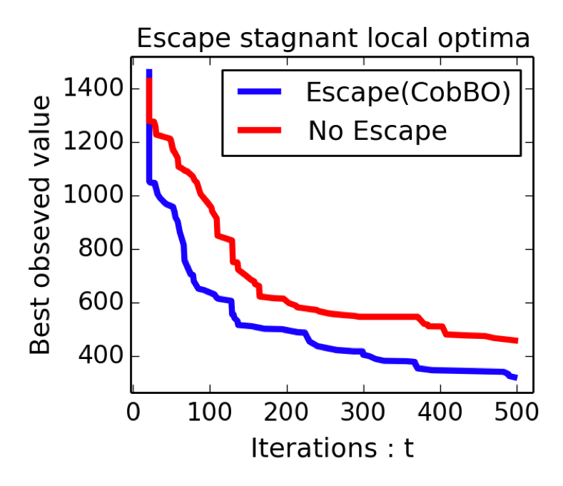
Figure 12: Ablation study for escaping local optima for Rastrigin on $[-5,10]^{50}$ with $20$ initial random samples.

We further the experiment with Levy and Ackley functions of 100 dimensions, as described in Section 4.2.1 to compute the fraction of queries that improve the already observed maximal points due to the change of $V_{t}$.

Problem	Average # improved queries	Average # improved queries due to escaping
Ackley	228	15.3
Levy	155	3

Table 1: The number of improved queries due to escaping local maxima

We observe that optimizing the Levy function yields very few queries that improve the maximal points by changing the pivot point, while optimizing the Ackley function can benefit more from that.

Appendix C Additional experiments

In Fig. 13 we show that CobBO also optimizes well the Michalewicz function on $10$ dimensions, although it has symmetric bumps, where certain subspaces pass through a point in a symmetrical manner and others break it.

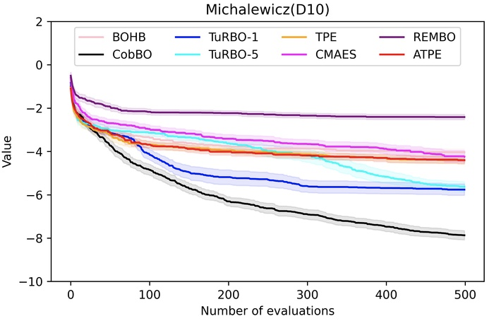
Figure 13: Performance over the low dimensional Michalewicz function with symmetrical and asymmetrical subspaces

Other real applications include parameter tuning for recommendation systems, database online performance tuning, and simulation based parameter optimization. However, due to deviating from the main study of this paper, we refrain from presenting these results that require elaborated description on the application backgrounds.

References

- Acerbi & Ma (2017) Acerbi, L. and Ma, W. J. Practical bayesian optimization for model fitting with bayesian adaptive direct search. In Proceedings of the 31st International Conference on Neural Information Processing Systems, NIPS’17, pp. 1834–1844, Red Hook, NY, USA, 2017. Curran Associates Inc. ISBN 9781510860964.
- Arora et al. (2012) Arora, S., Hazan, E., and Kale, S. The multiplicative weights update method: a meta-algorithm and applications. Theory of Computing, 8(6):121–164, 2012.
- Auer (2003) Auer, P. Using confidence bounds for exploitation-exploration trade-offs. J. Mach. Learn. Res., 3(null):397–422, March 2003. ISSN 1532-4435.
- Bergstra et al. (2011) Bergstra, J. S., Bardenet, R., Bengio, Y., and Kégl, B. Algorithms for hyper-parameter optimization. In Shawe-Taylor, J., Zemel, R. S., Bartlett, P. L., Pereira, F., and Weinberger, K. Q. (eds.), Advances in Neural Information Processing Systems 24, pp. 2546–2554. Curran Associates, Inc., 2011.
- Binois et al. (2020) Binois, M., Ginsbourger, D., and Roustant, O. On the choice of the low-dimensional domain for global optimization via random embeddings. Journal of Global Optimization, 76(1):69–90, January 2020.
- Buhmann (2003) Buhmann, M. D. Radial Basis Functions: Theory and Implementations. Cambridge Monographs on Applied and Computational Mathematics. Cambridge University Press, 2003.
- Bull (2011) Bull, A. D. Convergence rates of efficient global optimization algorithms. Journal of Machine Learning Research, 12(88):2879–2904, 2011.
- Cesa-Bianchi & Lugosi (2006) Cesa-Bianchi, N. and Lugosi, G. Prediction, learning, and games. Cambridge university press, 2006.
- Djolonga et al. (2013) Djolonga, J., Krause, A., and Cevher, V. High-dimensional gaussian process bandits. In Burges, C. J. C., Bottou, L., Welling, M., Ghahramani, Z., and Weinberger, K. Q. (eds.), Advances in Neural Information Processing Systems 26, pp. 1025–1033. Curran Associates, Inc., 2013.
- ElectricBrain (2018) ElectricBrain. Blog: Learning to optimize, 2018. URL https://www.electricbrain.io/post/learning-to-optimize.
- Eriksson et al. (2019) Eriksson, D., Pearce, M., Gardner, J., Turner, R. D., and Poloczek, M. Scalable global optimization via local bayesian optimization. In Advances in Neural Information Processing Systems 32, pp. 5496–5507. Curran Associates, Inc., 2019.
- Frazier (2018) Frazier, P. I. A tutorial on bayesian optimization, 2018.
- Frazier et al. (2008) Frazier, P. I., Powell, W. B., and Dayanik, S. A knowledge-gradient policy for sequential information collection. SIAM J. Control Optim., 47(5):2410–2439, September 2008. ISSN 0363-0129.
- Gilboa et al. (2013) Gilboa, E., Saatçi, Y., and Cunningham, J. P. Scaling multidimensional Gaussian processes using projected additive approximations. In Proceedings of the 30th International Conference on International Conference on Machine Learning - Volume 28, ICML’13, pp. I–454–I–461. JMLR.org, 2013.
- Gumerov & Duraiswami (2007) Gumerov, N. A. and Duraiswami, R. Fast radial basis function interpolation via preconditioned krylov iteration. SIAM Journal on Scientific Computing, 29(5):1876–1899, 2007.
- Hansen & Ostermeier (2001) Hansen, N. and Ostermeier, A. Completely derandomized self-adaptation in evolution strategies. Evolutionary Computation, 9(2):159–195, June 2001. ISSN 1063-6560.
- Haussler et al. (1995) Haussler, D., Kivinen, J., and Warmuth, M. K. Tight worst-case loss bounds for predicting with expert advice. In European Conference on Computational Learning Theory, pp. 69–83. Springer, 1995.
- Hennig & Schuler (2012) Hennig, P. and Schuler, C. J. Entropy search for information-efficient global optimization. J. Mach. Learn. Res., 13(1):1809–1837, June 2012. ISSN 1532-4435.
- Henrández-Lobato et al. (2014) Henrández-Lobato, J. M., Hoffman, M. W., and Ghahramani, Z. Predictive entropy search for efficient global optimization of black-box functions. In Proceedings of the 27th International Conference on Neural Information Processing Systems - Volume 1, NIPS’14, pp. 918–926, Cambridge, MA, USA, 2014. MIT Press.
- Jones et al. (1998) Jones, D. R., Schonlau, M., and Welch, W. J. Efficient global optimization of expensive black-box functions. Journal of Global optimization, 13(4):455–492, 1998.
- Kandasamy et al. (2015) Kandasamy, K., Schneider, J., and Póczos, B. High dimensional bayesian optimization and bandits via additive models. In Proceedings of the 32nd International Conference on International Conference on Machine Learning - Volume 37, ICML’15, pp. 295–304. JMLR.org, 2015.
- Kirschner et al. (2019) Kirschner, J., Mutny, M., Hiller, N., Ischebeck, R., and Krause, A. Adaptive and safe Bayesian optimization in high dimensions via one-dimensional subspaces. In Chaudhuri, K. and Salakhutdinov, R. (eds.), Proceedings of the 36th International Conference on Machine Learning, volume 97 of Proceedings of Machine Learning Research, pp. 3429–3438, Long Beach, California, USA, 09–15 Jun 2019. PMLR.
- Kushner (1964) Kushner, H. J. A new method of locating the maximum point of an arbitrary multipeak curve in the presence of noise. Journal of Basic Engineering, 86(1):97–106, mar 1964.
- Letham et al. (2020) Letham, B., Calandra, R., Rai, A., and Bakshy, E. Re-examining linear embeddings for high-dimensional bayesian optimization. In Larochelle, H., Ranzato, M., Hadsell, R., Balcan, M. F., and Lin, H. (eds.), Advances in Neural Information Processing Systems, volume 33, pp. 1546–1558. Curran Associates, Inc., 2020.
- Li et al. (2017) Li, C., Gupta, S., Rana, S., Nguyen, V., Venkatesh, S., and Shilton, A. High dimensional bayesian optimization using dropout. In Proceedings of the Twenty-Sixth International Joint Conference on Artificial Intelligence, IJCAI-17, pp. 2096–2102, 2017.
- McLeod et al. (2018) McLeod, M., Osborne, M. A., and Roberts, S. J. Optimization, fast and slow: Optimally switching between local and bayesian optimization. In ICML, 2018.
- Močkus (1975) Močkus, J. On bayesian methods for seeking the extremum. In Marchuk, G. I. (ed.), Optimization Techniques IFIP Technical Conference Novosibirsk, July 1–7, 1974, pp. 400–404, Berlin, Heidelberg, 1975. Springer Berlin Heidelberg. ISBN 978-3-540-37497-8.
- Moriconi et al. (2020) Moriconi, R., Kumar, K. S. S., and Deisenroth, M. P. High-dimensional bayesian optimization with projections using quantile gaussian processes. Optimization Letters, 14:51–64, 2020.
- Munteanu et al. (2019) Munteanu, A., Nayebi, A., and Poloczek, M. A framework for Bayesian optimization in embedded subspaces. In Chaudhuri, K. and Salakhutdinov, R. (eds.), Proceedings of the 36th International Conference on Machine Learning, volume 97 of Proceedings of Machine Learning Research, pp. 4752–4761, Long Beach, California, USA, 09–15 Jun 2019. PMLR.
- Mutny & Krause (2018) Mutny, M. and Krause, A. Efficient high dimensional bayesian optimization with additivity and quadrature fourier features. In Bengio, S., Wallach, H., Larochelle, H., Grauman, K., Cesa-Bianchi, N., and Garnett, R. (eds.), Advances in Neural Information Processing Systems 31, pp. 9005–9016. Curran Associates, Inc., 2018.
- Nutini et al. (July 2015) Nutini, J., Schmidt, M., Laradji, I. H., Friedlander, M., and Koepke, H. Coordinate descent converges faster with the gauss-southwell rule than random selection. ICML’15: Proceedings of the 32nd International Conference on International Conference on Machine Learning, 37, July 2015.
- Oh et al. (2018) Oh, C., Gavves, E., and Welling, M. BOCK : Bayesian optimization with cylindrical kernels. In Dy, J. and Krause, A. (eds.), Proceedings of the 35th International Conference on Machine Learning, volume 80 of Proceedings of Machine Learning Research, pp. 3868–3877, Stockholm, Sweden, 10–15 Jul 2018. PMLR.
- Oliveira et al. (2018) Oliveira, R., Rocha, F., Ott, L., Guizilini, V., Ramos, F., and Jr, V. Learning to race through coordinate descent bayesian optimisation. In IEEE International Conference on Robotics and Automation (ICRA), February 2018.
- (34) Radial basis function. https://docs.scipy.org/doc/scipy/reference/generated/scipy.interpolate.Rbf.html.
- Rahimi & Recht (2008) Rahimi, A. and Recht, B. Random features for large-scale kernel machines. In Platt, J. C., Koller, D., Singer, Y., and Roweis, S. T. (eds.), Advances in Neural Information Processing Systems 20, pp. 1177–1184. Curran Associates, Inc., 2008.
- Rasmussen & Williams (2005) Rasmussen, C. E. and Williams, C. K. I. Gaussian Processes for Machine Learning (Adaptive Computation and Machine Learning). The MIT Press, 2005. ISBN 026218253X.
- Scott et al. (2011) Scott, W., Frazier, P., and Powell, W. The correlated knowledge gradient for simulation optimization of continuous parameters using gaussian process regression. SIAM Journal on Optimization, 21(3):996–1026, 2011.
- Shepard (1968) Shepard, D. A two-dimensional interpolation function for irregularly-spaced data. In Proceedings of the 1968 23rd ACM National Conference, ACM ’68, pp. 517–524, New York, NY, USA, 1968. Association for Computing Machinery. ISBN 9781450374866.
- Srinivas et al. (2010) Srinivas, N., Krause, A., Kakade, S., and Seeger, M. Gaussian process optimization in the bandit setting: No regret and experimental design. In Proceedings of the 27th International Conference on International Conference on Machine Learning, ICML’10, pp. 1015–1022, Madison, WI, USA, 2010.
- Srinivas et al. (2012) Srinivas, N., Krause, A., Kakade, S. M., and Seeger, M. W. Information-theoretic regret bounds for gaussian process optimization in the bandit setting. IEEE Transactions on Information Theory, 58(5):3250–3265, 2012.
- Surjanovic & Bingham (2013) Surjanovic, S. and Bingham, D. Optimization test problems, 2013. URL http://www.sfu.ca/~ssurjano/optimization.html.
- Tyagi & Cevher (2014) Tyagi, H. and Cevher, V. Learning non-parametric basis independent models from point queries via low-rank methods. Applied and Computational Harmonic Analysis, 37(3):389 – 412, 2014. ISSN 1063-5203.
- Wang et al. (2020) Wang, L., Fonseca, R., and Tian, Y. Learning search space partition for black-box optimization using monte carlo tree search. ArXiv, abs/2007.00708, 2020.
- Wang & Jegelka (2017) Wang, Z. and Jegelka, S. Max-value entropy search for efficient Bayesian optimization. In Precup, D. and Teh, Y. W. (eds.), Proceedings of the 34th International Conference on Machine Learning, volume 70 of Proceedings of Machine Learning Research, pp. 3627–3635, International Convention Centre, Sydney, Australia, 06–11 Aug 2017. PMLR.
- Wang et al. (2016) Wang, Z., Hutter, F., Zoghi, M., Matheson, D., and De Freitas, N. Bayesian optimization in a billion dimensions via random embeddings. J. Artif. Int. Res., 55(1):361–387, January 2016. ISSN 1076-9757.
- Wang et al. (2017) Wang, Z., Li, C., Jegelka, S., and Kohli, P. Batched high-dimensional bayesian optimization via structural kernel learning. In Proceedings of the 34th International Conference on Machine Learning - Volume 70, ICML’17, pp. 3656–3664. JMLR.org, 2017.
- Wang et al. (2018) Wang, Z., Gehring, C., Kohli, P., and Jegelka, S. Batched large-scale bayesian optimization in high-dimensional spaces. In International Conference on Artificial Intelligence and Statistics (AISTATS), 2018.
- Wright (June 2015) Wright, S. J. Coordinate descent algorithms. Mathematical Programming: Series A and B, June 2015.
- Wu & Frazier (2016) Wu, J. and Frazier, P. I. The parallel knowledge gradient method for batch bayesian optimization. In Proceedings of the 30th International Conference on Neural Information Processing Systems, NIPS’16, pp. 3134–3142, Red Hook, NY, USA, 2016. Curran Associates Inc. ISBN 9781510838819.