Saturating PI Control of Stable Nonlinear Systems Using Singular Perturbations

Abstract

This paper presents an anti-windup PI controller, using a saturating integrator, for a single-input single-output stable nonlinear plant, whose steady-state input-output map is increasing. We prove that, under reasonable assumptions, there exists an upper bound on the controller gain such that for any constant reference input, the corresponding equilibrium point of the closed-loop system is exponentially stable, with a “large” region of attraction. When the state of the closed-loop system converges to this equilibrium point, then the tracking error tends to zero. The closed-loop stability analysis employs Lyapunov methods in the framework of singular perturbations theory. Finally, we show that if the plant satisfies the asymptotic gain property, then the closed-loop system is globally asymptotically stable for any sufficiently small controller gain. The effectiveness of the proposed PI controller is proved by showing how it performs as part of the control algorithm of a synchronverter (a special type of DC to AC power converter).

I Introduction

PProportional-integral (PI) control is extensively used to achieve robust asymptotic tracking and disturbance rejection of constant external signals (it is the simplest instance of the internal model principle). When the plant is an uncertain linear system, closed-loop stability can be achieved if the control gains are sufficiently small and the plant fulfils certain stability conditions [10, 35]. The theory has been extended to nonlinear systems, where global results have been derived in [7] for PI control and in [40] for integral control, and local ones in [19] for the more general internal model principle. Later, regional and semiglobal results have been presented in [18], [23] for specific classes of nonlinear systems using high-gain observers. For extensions of PI control to infinite dimensional linear systems see [13, 31, 38].

In the presence of actuator limitations, e.g. saturation, there can be a mismatch between the actual plant input and the controller output. When this happens, the controller output does not drive the plant and, as a result, the states of the controller are wrongly updated. If the controller is unstable (such as PI), then the state of the controller may reach a region far from the normal operating range, an effect called controller windup [27]. (Windup can also be caused by a temporary fault in the system.) Windup may cause long transients, oscillations and even instability. To prevent windup, several anti-windup techniques have been investigated in the last 50 years. Mainly, two design approaches can be identified (see [45]): one-step design, where both the actuator limitations and the performances are taken into account during the controller design, and two-steps design (also known as anti-windup compensation), where first a nominal controller is designed ignoring the actuator nonlinearities, focusing on the performance, and then an anti-windup compensator is added to handle the actuator nonlinearities so that the closed-loop performance degrades “gracefully” when actuator limitations occur.

In the field of linear systems, one of the first systematic anti-windup methods is the conditioning technique introduced in [14] as an extension of the back calculation method presented in [9]. Later, this and other designs have been collected in [1], where the more general observer approach is formulated for a class of anti-windup compensation schemes, which includes the conditioning technique. For the application of internal model control to the anti-windup problem, see [51]. Even though this method does not excel in terms of performance, it has been proved later (see [46]) to be the optimal one in terms of robustness. One of the first theoretical frameworks for the study of two-steps anti-windup design for LTI systems is in [27], where a general coprime-factor scheme is introduced, unifying all the known anti-windup methods. Related later work is in [8], where a generic approach in the form of an $H_{\infty}$ optimization framework is proposed. A comprehensive review of anti-windup techniques specific for PID controllers is [49]. Additional results on anti-windup schemes for PI and PID controllers are respectively in [5], where the conditional integrator scheme is improved by setting a specific initial value for the integrator when switching from P to PI control mode, and in [16], where a variable structure PID is presented, able to switch between normal operating mode and anti-windup compensator mode. A recent result on anti-windup low-gain integral control for multivariable linear systems subject to input nonlinearities is in [12]. A treatment of the ${\mathscr{L}}_{2}$ anti-windup problem is in [50]. In recent years, more attention has been devoted to LMIs to tackle complex anti-windup scenarios. In fact, the actuator nonlinearities can be modelled as sector nonlinearities so that the anti-windup controller design is recast into a convex optimization problem under LMI constraints [45]. In this context, in [46] the uncertainty in the system model is taken into account, and in [48] regional stability is guaranteed in the presence of input saturation for an exponentially unstable linear system. These and other LMI-based methods can be found in the comprehensive surveys [15, 44, 45].

Nonlinear systems have received less attention in the anti-windup literature. The first notable results in this direction are based on input-output linearization techniques, combined with internal model control, for nonlinear affine systems. Among them, we refer to [17] for single-input-single-output nonlinear systems and to [20, 22] for multivariable systems. For Euler-Lagrange systems, an anti-windup scheme inducing global asymptotic stability and local exponential stability is proposed in [34]. For LMI-based optimization techniques, the reader is referred to [6], [39], and the references therein.

A one-step anti-windup design for nonlinear systems has been recently proposed in [26], where a bounded integral controller (BIC) is presented. Under suitable assumptions (input to state practical stability), the BIC generates a bounded control signal, guaranteeing boundedness of the plant state trajectory, while achieving tracking for constant references. According to [26], most integral control algorithms for nonlinear plants require detailed knowledge of the plant, leading to high complexity. Therefore, a simple anti-windup controller that allows a rigorous stability analysis, based on simple assumptions about the plant, is of significance.

This paper proposes a one-step anti-windup PI design for stable nonlinear systems. This PI controller uses a saturating integrator, which ensures that the integrator state is constrained to a compact interval chosen based on physical constraints. The saturating integrator is straightforward to implement and it has proved to be effective in power electronics applications, see for instance [28], [30] and [36]. Our main result, Theorem IV.3, shows that under reasonable assumptions, for small enough controller gain, the closed-loop system is (locally) exponentially stable and the region of attraction of its equilibrium point contains a curve of equilibrium points of the open-loop system.

Note that results closely related to our Theorem IV.3, considering only integral control, with many proofs missing, and without using singular perturbation theory, have been presented in the conference paper [47]. We believe that the new singular perturbations approach is much more elegant, and more suitable for generalizations. A preliminary and partial presentation of our results, without applications, is in our recent conference paper [33], again considering only integral control. Moreover, the global stability results from Section V here are substantially stronger than those in [33].

The paper is organized as follows. In Section II the saturating integrator is introduced and the control system under consideration is described in precise terms. In Section III the closed-loop system equations are rewritten as a singular perturbation model. In Section IV the main result is presented, with the stability analysis of the closed-loop system using singular perturbation methods. In Section V we assume that the plant satisfies the asymptotic gain property around each equilibrium point. Then, we show that for small enough controller gain, the closed-loop system is globally asymptotically stable. Finally, in Section VI we illustrate our theory using two examples: a toy example and a real application in the control of a certain type of three phase inverters.

II The closed-loop system

We describe the control system that will be investigated here. The nonlinear plant ${\mathbf{P}}$ to be controlled is described by:

$$\dot{x}{\hbox{\hskip 1.0pt}}={\hbox{\hskip 1.0pt}}f(x,u),\qquad y{\hbox{\hskip 1.0pt}}={\hbox{\hskip 1.0pt}}g(x),$$ (1)

where $f\in C^{2}({\mathbb{R}}^{n}\times{\mathbb{R}};{\mathbb{R}}^{n})$ and $g\in{\rm Lip}({\mathbb{R}}^{n};{\mathbb{R}})$. In this paper, Lip denotes a space of locally Lipschitz functions, that is, functions that are Lipschitz on any compact set.

The control objective is to make the output signal $y$ track a constant reference signal $r\in Y\vcentcolon=[y_{min},y_{max}]\subset{\mathbb{R}}$, using an input signal that in steady state takes values in the range $U\vcentcolon=[u_{min},u_{max}]\subset\mathbb{R}$ (here $u_{min}<u_{max}$). In order to achieve this goal, a type of anti-windup integral controller is used, which we call the saturating integrator. We define the positive (negative) part of a real number $w$ by $w^{+}=\max\{w,0\}$ ($w^{-}=\min\{w,0\}$), so that $w=w^{+}+w^{-}$. The saturating integrator is a system with input $w$ and state $u_{I}$, described by

$$\begin{gathered}\dot{u}_{I}{\hbox{\hskip 1.0pt}}={\hbox{\hskip 1.0pt}}{\mathscr{S}}(u_{I},w),\\ {\hbox{\hskip 1.0pt}}\text{where}\qquad{\mathscr{S}}(u_{I},w){\hbox{\hskip 1.0pt}}={\hbox{\hskip 1.0pt}}\begin{cases}w^{+}&\text{if}\quad u_{I}\leq u_{min},\\ w&\text{if}\quad u_{I}\in(u_{min},u_{max}),\\ w^{-}&\text{if}\quad u_{I}\geq u_{max}.\end{cases}\end{gathered}$$ (2)

The idea behind (2) is that if $u_{I}\geq u_{max}$ ($u_{I}\leq u_{min}$), we do not allow $u_{I}$ to move further into the forbidden region. In this way, assuming that $u_{I}(0)\in U$, the state trajectory $u_{I}(t)$ is constrained in $U$ for all $t\geq 0$. A similar controller is described in [16], under the name of conditionally freeze integrator, however no closed-loop stability results are given. We also mention that the limited integrator present in the MATLAB/Simulink software is of the form (2).

Remark II.1

As discussed in [3], the saturating integrator (2) can be approximated by the nonlinear system with input $w$, state $v_{I}$ and output $\bar{v}_{I}$ described by

$$\dot{v}_{I}=w-\lambda(v_{I}-\bar{v}_{I}),\qquad\bar{v}_{I}={\rm sat}{\hbox{\hskip 1.0pt}}v_{I},\vspace{-1mm}$$

where ${\rm sat}$ is the saturating function with lower bound $u_{min}$ and upper bound $u_{max}$, and the gain $\lambda>0$ is sufficiently large. More precisely, as stated in [3, Lemma 5.1], the approximation error $e_{I}\vcentcolon=\bar{v}_{I}-u_{I}$, where $u_{I}$ is the state of (2), tends to zero for increasing values of $\lambda$. The advantage of this representation is that, in case of a linear plant ${\mathbf{P}}$, the stability analysis can be performed using the LMI-based tools developed, for instance, in [3, 41, 45, 44].

As shown in Fig. 1, we connect the saturating integrator in parallel with a proportional gain $\tau_{p}\geq 0$, and the input to these two blocks comes through a gain $k>0$. If the integrator does not saturate, then this is a linear PI controller with transfer function

$${\mathbf{C}}(s){\hbox{\hskip 1.0pt}}={\hbox{\hskip 1.0pt}}k\left(\tau_{p}+\frac{1}{s}\right){\hbox{\hskip 1.0pt}}.$$ (3)

(Here $\tau_{p}\geq 0$ is considered to be given, while $k>0$ to be chosen according to the discussion in Remark IV.4.) We assume that $r\in Y$. Most of the time we have that $u(t)\in U$, thanks to the saturating integrator, and thanks to the fact that in steady state, $e(t)=0$. During transients the signal $u$ may exit $U$ because of the term $\tau_{p}w$, but $u_{I}$ will remain in $U$. The closed-loop system from Fig. 1 is given by

$$\begin{cases}\begin{gathered}{\hbox{\hskip 1.0pt}}\ \dot{x}{\hbox{\hskip 1.0pt}}={\hbox{\hskip 1.0pt}}f(x,u_{I}+\tau_{p}k(r-g(x))),\\ \dot{u}_{I}{\hbox{\hskip 1.0pt}}={\hbox{\hskip 1.0pt}}{\mathscr{S}}(u_{I},k(r-g(x))),\end{gathered}\end{cases}$$ (4)

with state $(x,u_{I})$ and state space $X\vcentcolon={\mathbb{R}}^{n}\times U$.

An informal statement of our main result (see Theorem IV.3) is that, under reasonable assumptions on the plant ${\mathbf{P}}$, the following holds: For any small enough $k>0$, the closed-loop system (4) shown in Fig. 1, with any constant reference $r\in Y$, is locally exponentially stable around an equilibrium point, with a “large” region of attraction. When the state converges to this equilibrium point, then the tracking error $e\vcentcolon=r-y$ tends to zero at an exponential rate. Moreover, this result remains true also if $r$ has finitely many step changes, if the time interval between consecutive changes is large enough.

A related result, but without limitations on $u$, assuming global exponential stability of the plant’s equilibrium point for any constant input $u\in\mathbb{R}^{m}$, has been given in [7]. Recently, the result from [7] has been generalized in [40], where the assumption on the monotonicity of the plant steady-state input-output map has been replaced by the (weaker) uniform infinitesimal contracting property of the reduced dynamics.

Figure 1: Closed-loop system formed by the plant ${\mathbf{P}}$, the saturating integrator $\int{\mathscr{S}}$ and the constant gains $k>0$, $\tau_{p}\geq 0$, with the reference $r$.

Before addressing the stability analysis of the closed-loop system (4), some care has to be taken to define its trajectories. First, it has to be ensured that the state trajectories $u_{I}$ of the saturating integrator (2) are well-defined for any input $w\in L^{1}[0,t]$. For this we resort to a density argument: Note that for a polynomial input $w$, the state trajectory $u_{I}$ is easy to define. (The key is that a polynomial has finitely many zeros. Problems with defining the solution of (2) may arise when the zeros of $w$ have an accumulation point, for instance if $w(t)=t\sin(\frac{1}{t})$ and $u_{I}(0)=u_{max}$.)

Let $u_{1},u_{2}$ be the state trajectories of (2) corresponding to the polynomials $w_{1},w_{2}$. Then by an elementary argument

$$\lvert u_{2}(t)-u_{1}(t)\rvert\leq\lvert u_{2}(0)-u_{1}(0)\rvert+\int_{0}^{t}\lvert w_{2}(\sigma)-w_{1}(\sigma)\rvert d\sigma.$$ (5)

This shows that $u_{I}(t)$ depends Lipschitz continuously both on $u_{I}(0)$ and also on $w$ considered with the $L^{1}$ norm. For $u_{2}(0)=u_{1}(0)$ we can write the last estimate as

$$|u_{2}(t)-u_{1}(t)|\leq\|w_{2}-w_{1}\|_{L^{1}[0,t]}.$$ (6)

Hence, by continuous extension, we can define $u_{I}(t)$ for any initial state $u_{I}(0)$ and for any input $w\in L^{1}[0,t]$ (because the polynomials are dense in $L^{1}[0,t]$). Next, we show the local existence and uniqueness of the state trajectories of (4), which is not trivial due to the discontinuity of $\mathscr{S}$.

Notation. For any $\delta>0$, denote $U_{\delta}\vcentcolon=[u_{min}-\delta,u_{max}+\delta]$.

Proposition II.2

Let ${\mathbf{P}}$ be described by (1) and let $\int{\mathscr{S}}$ be the saturating integrator from (2). For every $k,\tau_{p}\in\mathbb{R}$, $x_{0}\in{\mathbb{R}}^{n}$, $\delta>0$, $u_{0}\in U_{\delta}$, and every constant $r\in{\mathbb{R}}$ there exists a $\tau\in(0,\infty]$ such that the closed-loop system (4) (shown in Fig. 1) has a unique state trajectory $(x,u_{I})$ defined on $[0,\tau)$, such that $x(0)=x_{0}$ and $u_{I}(0)=u_{0}$. If $\tau$ is finite and maximal (i.e., the state trajectory cannot be continued beyond $\tau$), then $\limsup_{t\mathop{\rightarrow}\tau}\|x(t)\|=\infty$.

For the proof see Appendix A.

III Formulation as a standard singular perturbation model

To perform the stability analysis of the closed-loop system (4), the idea is to regard the constant gain $k>0$ as a “sufficiently small” parameter such that (4) can be rewritten as a standard singular perturbation model (see [25, Chapt. 1] or [24, Chapt. 11]). Then, we can separately analyze the stability of the reduced (slow) model and of the boundary-layer (fast) system, and, using the tools from singular perturbation theory, obtain stability results for (4). Note that in the less general formulation in [24, Sect. 11.5], the functions determining the closed-loop system are required to be locally Lipschitz, while in [25, Chapt. 7] it is only required that a unique (local) solution exists for the closed-loop system, which we have proved in Proposition II.2.

The following assumption is common in the singular perturbation theory (see [7],[40], [24, Chapt. 11], [25]) and in the theory for nonlinear systems with slowly varying inputs (see [21], [29], [24, Sect. 9.6]).

Assumption 1

There exists $\delta>0$ and a function $\Xi\in C^{1}(U_{\delta};{\mathbb{R}}^{n})$ such that $$f(\Xi(u),u){\hbox{\hskip 1.0pt}}={\hbox{\hskip 1.0pt}}0{\hbox{$\hskip 31.29802pt\forall\;$}}u\in U_{\delta},\vspace{-1mm}$$ (7) i.e., for each $u_{0}\in U_{\delta}$, $\Xi(u_{0})$ is an equilibrium point that corresponds to the constant input $u_{0}$. Moreover, ${\mathbf{P}}$ is uniformly exponentially stable around these equilibrium points. This means that there exist ${\varepsilon}_{0}>0$, ${\lambda}>0$ and $m\geq 1$ such that for each constant input function $u_{0}\in U_{\delta}$, the following holds for the solutions of (1): If $\lVert x(0)-\Xi(u_{0})\rVert\leq{\varepsilon}_{0}$, then for every $t\geq 0$, $$\lVert x(t)-\Xi(u_{0})\rVert\leq me^{-{\lambda}t}\lVert x(0)-\Xi(u_{0})\rVert.$$ (8)

Remark III.1

The uniform exponential stability condition above can be checked by linearization: If the Jacobian matrices

$$A(u_{0}){\hbox{\hskip 1.0pt}}={\hbox{\hskip 1.0pt}}\left.\frac{\partial f(x,u)}{\partial x}\right|_{{\hbox{\hskip-3.0pt}}\begin{array}[]{c}\scriptstyle x=\Xi(u_{0})\vspace{-1mm}\\ \scriptstyle u=u_{0}\end{array}}{\hbox{\hskip 1.0pt}}\in{\hbox{\hskip 1.0pt}}{\mathbb{R}}^{n\times n}\vspace{-1mm}$$ (9)

have eigenvalues bounded away from the right half-plane,

$$\max{\rm Re\,}\sigma(A(u_{0})){\hbox{\hskip 1.0pt}}\leq{\hbox{\hskip 1.0pt}}{\lambda}_{0}{\hbox{\hskip 1.0pt}}<{\hbox{\hskip 1.0pt}}0{\hbox{$\hskip 31.29802pt\forall\;$}}u_{0}\in U_{\delta},$$

then ${\mathbf{P}}$ is uniformly exponentially stable, see (11.16) in [24]. From the first part of Assumption 1, $\max{\rm Re\,}\sigma(A(u_{0}))$ is a continuous function of $u_{0}$. Hence, if this function is always negative, then by the compactness of $U_{\delta}$, its maximum is also negative. Thus, for the uniform exponential stability of ${\mathbf{P}}$ we only have to check that each of the matrices $A(u_{0})$ is stable (where $u_{0}\in U_{\delta}$).

Remark III.2

If there exists a function $\Xi$ with the properties (7) and (8), then automatically $\Xi\in C^{2}$ according to the implicit function theorem, since $f\in C^{2}$. The stability property (8) guarantees that all the eigenvalues of the Jacobians from (9) are non-zero, see Remark III.1.

Assumption 2

The system ${\mathbf{P}}$ satisfies Assumption 1 and, moreover, the function $$G(u)\vcentcolon=g(\Xi(u)){\hbox{$\hskip 31.29802pt\forall\;$}}u\in U_{\delta},$$ is monotone increasing in the following sense: there exists $\mu>0$ such that $$G(b)-G(a){\hbox{\hskip 1.0pt}}\geq{\hbox{\hskip 1.0pt}}\mu(b-a){\hbox{$\hskip 31.29802pt\forall\;$}}a,b\in U_{\delta},\ a<b{\hbox{\hskip 1.0pt}}.$$

Note that the function $G\in{\rm Lip}(U_{\delta},{\mathbb{R}})$. We denote $y_{min}\vcentcolon=G(u_{min})$ and $y_{max}\vcentcolon=G(u_{max})$, where clearly $y_{min}<y_{max}$. Moreover, using the notation $Y=[y_{min},y_{max}]$, for any $r\in Y$, we define $u_{r}\vcentcolon=G^{-1}(r)$, which is well-defined in $U$ since $G$ is continuous and strictly monotone.

Remark III.3

If ${\mathbf{P}}$ is linear, described by the matrices $A,B,C$ in the usual way ($\dot{x}=Ax+Bu$, $y=Cx$), then Assumption 1 reduces to the fact that $A$ is stable. The functions $\Xi$ and $G$ from Assumptions 1 and 2 are given by

$$\Xi(u){\hbox{\hskip 1.0pt}}={\hbox{\hskip 1.0pt}}(-A)^{-1}Bu,\qquad G(u){\hbox{\hskip 1.0pt}}={\hbox{\hskip 1.0pt}}P(0)u,$$

where $P(s)=C(sI-A)^{-1}B$ is the plant transfer function. Assumption 2 is satisfied if and only if $P(0)=\mu>0$. Note that the above conditions are the same conditions given in [35] for the closed-loop stability of a linear (stable) plant connected in feedback with a low-gain integral controller, when $k>0$.

Assumptions 1 and 2 are crucial for the stability analysis presented in Section IV. In fact, Assumption 1 guarantees the stability of the boundary-layer (fast) system, while Assumption 2 guarantees the stability of the reduced (slow) model. Note that $G$ is the steady-state input-output map associated to ${\mathbf{P}}$.

In the following, we manipulate the closed-loop equations (4) to rewrite them as a standard singular perturbation model (see (11.47), (11.48) in [24]). Defining the function

$$\beta(x,u_{I},k){\hbox{\hskip 1.0pt}}\vcentcolon={\hbox{\hskip 1.0pt}}f(x,u_{I}+\tau_{p}k(r-g(x)))-f(x,u_{I}),$$ (10)

the closed-loop system (4) can be rewritten as

$$\begin{cases}\begin{gathered}{\hbox{\hskip 1.0pt}}\ {\hbox{\hskip 1.0pt}}\dot{x}{\hbox{\hskip 1.0pt}}={\hbox{\hskip 1.0pt}}f(x,u_{I})+\beta(x,u_{I},k),\\ {\hbox{\hskip 1.0pt}}\dot{u}_{I}{\hbox{\hskip 1.0pt}}={\hbox{\hskip 1.0pt}}{\mathscr{S}}(u_{I},k(r-g(x))).\end{gathered}\end{cases}$$ (11)

Note that $\beta(x,u_{I},0)=0$ for all $(x,u_{I})\in\mathbb{R}^{n+1}$. We define

$$h(x,u_{I})\vcentcolon={\hbox{\hskip 1.0pt}}{\mathscr{S}}(u_{I},r-g(x)),$$ (12)

and then the closed-loop system (11) can be rewritten as

$$\dot{u}_{I}{\hbox{\hskip 1.0pt}}={\hbox{\hskip 1.0pt}}k\cdot h(x,u_{I}),\quad\dot{x}{\hbox{\hskip 1.0pt}}={\hbox{\hskip 1.0pt}}f(x,u_{I})+\beta(x,u_{I},k).$$ (13)

The functions $h(\cdot,\cdot)$ and $\beta(\cdot,\cdot,k)$ are defined on ${\mathbb{R}}^{n}\times U_{\delta}$. Using that $k>0$, we change the time-scale of (13) introducing $s\vcentcolon=kt$ (it is a “slower” time-scale because $k$ is small). Rewriting the system (13) in the new time-scale $s$, we get

$$\frac{{\rm d}\hbox{\hskip 0.5pt}u_{I}}{{\rm d}\hbox{\hskip 0.5pt}s}{\hbox{\hskip 1.0pt}}={\hbox{\hskip 1.0pt}}h(x,u_{I}),\quad k\frac{{\rm d}\hbox{\hskip 0.5pt}x}{{\rm d}\hbox{\hskip 0.5pt}s}{\hbox{\hskip 1.0pt}}={\hbox{\hskip 1.0pt}}f(x,u_{I})+\beta(x,u_{I},k).$$ (14)

To simplify the stability analysis, we move the equilibrium point of the closed-loop system (14) to the origin. It follows from Assumption 1 and the notation introduced after Assumption 2 that $(x_{r},u_{r})$ is an equilibrium point of (14), where $x_{r}\vcentcolon=\Xi(u_{r})$. Note that $g(x_{r})=r$. Introduce the variables

$$\tilde{x}{\hbox{\hskip 1.0pt}}\vcentcolon={\hbox{\hskip 1.0pt}}x-x_{r},\qquad\tilde{u}_{I}\vcentcolon={\hbox{\hskip 1.0pt}}u_{I}-u_{r},$$ (15)

and the functions

$$\tilde{h}(\tilde{u}_{I},\tilde{x})\vcentcolon={\hbox{\hskip 1.0pt}}h(\tilde{x}+x_{r},\tilde{u}_{I}+u_{r}),$$ (16a)

$$\tilde{f}(\tilde{u}_{I},\tilde{x})\vcentcolon={\hbox{\hskip 1.0pt}}f(\tilde{x}+x_{r},\tilde{u}_{I}+u_{r}),$$ (16b)

$$\tilde{g}(\tilde{x})\vcentcolon=g(\tilde{x}+x_{r}),$$ (16c)

$$\tilde{\beta}(\tilde{u}_{I},\tilde{x},k)\vcentcolon={\hbox{\hskip 1.0pt}}\tilde{f}(\tilde{u}_{I}+\tau_{p}k(r-\tilde{g}(\tilde{x})),\tilde{x})-\tilde{f}(\tilde{u}_{I},\tilde{x})$$ (16d)

$$={\hbox{\hskip 1.0pt}}\beta(\tilde{x}+x_{r},\tilde{u}_{I}+u_{r},k).$$

The system (14) can be rewritten as

$$\frac{{\rm d}\hbox{\hskip 0.5pt}\tilde{u}_{I}}{{\rm d}\hbox{\hskip 0.5pt}s}{\hbox{\hskip 1.0pt}}={\hbox{\hskip 1.0pt}}\tilde{h}(\tilde{u}_{I},\tilde{x}),\qquad k\frac{{\rm d}\hbox{\hskip 0.5pt}\tilde{x}}{{\rm d}\hbox{\hskip 0.5pt}s}{\hbox{\hskip 1.0pt}}={\hbox{\hskip 1.0pt}}\tilde{f}(\tilde{u}_{I},\tilde{x})+\tilde{\beta}(\tilde{u}_{I},\tilde{x},k),$$ (17)

with an equilibrium point $(\tilde{u}_{I},\tilde{x})=(0,0)$. For $k>0$ small, this is a standard singular perturbation model according to [24, Sect. 11.5] (see equations (11.47) and (11.48) there). Note that in our case the system (17) is autonomous.

TABLE I: Correspondence of our notation with the one used in [24]

this paper	$\tilde{u}_{I}$	$\tilde{x}$	$\tilde{h}$	$\tilde{f}+\tilde{\beta}$	$k$	$z$	$\tilde{\Xi}$	$s$	$t$	${\varepsilon}_{0}$
[24]	$x$	$z$	$f$	$g$	${\varepsilon}$	$y$	$h$	$t$	$\tau$	$r_{0}$

Recalling $\Xi$ from Assumption 1, we introduce the function

$$\tilde{\Xi}(\tilde{u}_{I})\vcentcolon={\hbox{\hskip 1.0pt}}\Xi(\tilde{u}_{I}+u_{r})-x_{r}$$ (18)

and following the guidelines of [24], we define

$$z\vcentcolon={\hbox{\hskip 1.0pt}}\tilde{x}-\tilde{\Xi}(\tilde{u}_{I})=x-\Xi(u_{I}).$$ (19)

Using the notation introduced above, we reformulate our system (17) like (11.49), (11.50) of [24], i.e.,

$$\frac{{\rm d}\hbox{\hskip 0.5pt}\tilde{u}_{I}}{{\rm d}\hbox{\hskip 0.5pt}s}{\hbox{\hskip 1.0pt}}={\hbox{\hskip 1.0pt}}\tilde{h}(\tilde{u}_{I},z+\tilde{\Xi}(\tilde{u}_{I})),$$ (20)

$$k\frac{{\rm d}\hbox{\hskip 0.5pt}z}{{\rm d}\hbox{\hskip 0.5pt}s}{\hbox{\hskip 1.0pt}}={\hbox{\hskip 1.0pt}}\tilde{f}(\tilde{u}_{I},z+\tilde{\Xi}(\tilde{u}_{I}))+\tilde{\beta}(\tilde{u}_{I},z+\tilde{\Xi}(\tilde{u}_{I}),k)\\ -k\frac{{\rm d}\hbox{\hskip 0.5pt}\tilde{\Xi}}{{\rm d}\hbox{\hskip 0.5pt}\tilde{u}_{I}}\tilde{h}(\tilde{u}_{I},z+\tilde{\Xi}(\tilde{u}_{I})),$$ (21)

which has an equilibrium point at $(\tilde{u}_{I},z)=(0,0)$. Finally, in accordance with the change of variables (15), we define

$$\tilde{u}_{min}\vcentcolon={\hbox{\hskip 1.0pt}}u_{min}-u_{r}{\hbox{\hskip 1.0pt}},\qquad\tilde{u}_{max}\vcentcolon={\hbox{\hskip 1.0pt}}u_{max}-u_{r}$$

and the sets $\tilde{U}\vcentcolon=[\tilde{u}_{min},\tilde{u}_{max}]\subset{\mathbb{R}}$, and

$$\tilde{U}_{\delta}\vcentcolon=[\tilde{u}_{min}-\delta,\tilde{u}_{max}+\delta]{\hbox{\hskip 1.0pt}}.$$

$\tilde{U}_{\delta}$ contains 0 in its interior. The state space of the closed-loop system (20)-(21) is $\tilde{X}_{\delta}\vcentcolon=\tilde{U}_{\delta}\times{\mathbb{R}}^{n}$. To facilitate the comparison of our equations with those in [24], the relation between the notation in these two works is shown in Table I.

Remark III.4

Since $\tilde{\Xi}\in C^{2}(\tilde{U}_{\delta},{\mathbb{R}}^{n})$, the change of variables (19) is stability preserving, i.e., the origin of (20)-(21) is asymptotically (exponentially) stable, if and only if the origin of (17) is asymptotically (exponentially) stable.

The reduced (slow) model is obtained setting $k=0$ in (21), and solving the resulting algebraic equation

$$0{\hbox{\hskip 1.0pt}}={\hbox{\hskip 1.0pt}}\tilde{f}(\tilde{u}_{I},z+\tilde{\Xi}(\tilde{u}_{I})),$$

for which $z=0$ is a solution. Substituting $z=0$ in (20), the following reduced (slow) model is obtained:

$$\frac{{\rm d}\hbox{\hskip 0.5pt}\tilde{u}_{I}}{{\rm d}\hbox{\hskip 0.5pt}s}{\hbox{\hskip 1.0pt}}={\hbox{\hskip 1.0pt}}\tilde{h}(\tilde{u}_{I},\tilde{\Xi}(\tilde{u}_{I})).$$ (22)

Recall ${\mathscr{S}}$ from (2) and $G$ from Assumption 2. Defining

$$\begin{gathered}\tilde{\mathscr{S}}(\tilde{u}_{I},\cdot)\vcentcolon={\hbox{\hskip 1.0pt}}{\mathscr{S}}(\tilde{u}_{I}+u_{r},\cdot),\quad\tilde{G}(\tilde{u}_{I})\vcentcolon={\hbox{\hskip 1.0pt}}G(\tilde{u}_{I}+u_{r}),\end{gathered}$$

the reduced model (22) can be described equivalently (recall the definitions of $\tilde{h}$ from (16a) and of $h$ from (12)) by

$$\frac{{\rm d}\hbox{\hskip 0.5pt}\tilde{u}_{I}}{{\rm d}\hbox{\hskip 0.5pt}s}{\hbox{\hskip 1.0pt}}={\hbox{\hskip 1.0pt}}\tilde{{\mathscr{S}}}(\tilde{u}_{I},r-\tilde{G}(\tilde{u}_{I})).$$ (23)

The reduced closed-loop system is shown in Fig. 2. Note that

$$\tilde{h}(\tilde{u}_{I},\tilde{x}){\hbox{\hskip 1.0pt}}={\hbox{\hskip 1.0pt}}\tilde{{\mathscr{S}}}(\tilde{u}_{I},r-\tilde{g}(\tilde{x})).$$

Figure 2: Closed-loop representation of the reduced (slow) model (23).

The boundary-layer (fast) system is obtained by rewriting the second equation in (17) in the original fast time-scale $t$ as

$$\dot{z}{\hbox{\hskip 1.0pt}}={\hbox{\hskip 1.0pt}}\tilde{f}(\tilde{u}_{I},z+\tilde{\Xi}(\tilde{u}_{I}))+\tilde{\beta}(\tilde{u}_{I},z+\tilde{\Xi}(\tilde{u}_{I}),k).$$

Taking here $k=0$, we obtain the boundary-layer system

$$\dot{z}{\hbox{\hskip 1.0pt}}={\hbox{\hskip 1.0pt}}\tilde{f}(\tilde{u}_{I},z+\tilde{\Xi}(\tilde{u}_{I})),$$ (24)

where $\tilde{u}_{I}\in\tilde{U}_{\delta}$ is treated as a fixed parameter.

IV Stability analysis via singular perturbations

To perform the stability analysis of the closed-loop system (17), we would like to use Theorem 11.4 from [24]. However, the assumptions of this theorem are not met by our model. Therefore, we state a slightly modified version of it, which holds in our framework, together with a proof. Note that a similar result, with asymptotic stability in place of exponential one, is provided in Theorem 5.1 from [25, Chapt. 7].

The analysis will be performed by first finding two distinct Lyapunov functions $V$ and $W$, respectively for the reduced (slow) model (22) and the boundary-layer (fast) system (24). Then, our modified version of Theorem 11.4 from [24] will be stated, see Theorem IV.2. The stability of the closed-loop system (4), with the region of attraction containing the curve $\{(\Xi(u),u){\hbox{\hskip 1.0pt}}|{\hbox{\hskip 1.0pt}}u\in U\}$, will be presented in Theorem IV.3.

IV-A Stability of the reduced (slow) model

Our Theorem IV.2 requires the existence of a Lyapunov function $V$ for (22) (defined on $\tilde{U}_{\delta}$) such that

$$\begin{gathered}c_{1}\tilde{u}_{I}^{2}\leq V(\tilde{u}_{I})\leq c_{2}\tilde{u}_{I}^{2},\\ \frac{{\rm d}\hbox{\hskip 0.5pt}V}{{\rm d}\hbox{\hskip 0.5pt}\tilde{u}_{I}}\tilde{h}(\tilde{u}_{I},\tilde{\Xi}(\tilde{u}_{I}))\leq-c_{3}\lvert\tilde{u}_{I}\rvert^{2},\ \ \ \bigg{|}\frac{{\rm d}\hbox{\hskip 0.5pt}V}{{\rm d}\hbox{\hskip 0.5pt}\tilde{u}_{I}}\bigg{|}\leq c_{4}\lvert\tilde{u}_{I}\rvert,\end{gathered}$$ (25)

for all $\tilde{u}_{I}\in\tilde{U}_{\delta}$, where $c_{1},\dots c_{4}$ are positive constants. Consider the candidate

$$V(\tilde{u}_{I}){\hbox{\hskip 1.0pt}}={\hbox{\hskip 1.0pt}}\frac{1}{2}\tilde{u}_{I}^{2}{\hbox{$\hskip 31.29802pt\forall\;$}}\tilde{u}_{I}\in\tilde{U}_{\delta}.$$ (26)

It follows from (23) that

$$\frac{{\rm d}\hbox{\hskip 0.5pt}V}{{\rm d}\hbox{\hskip 0.5pt}s}{\hbox{\hskip 1.0pt}}={\hbox{\hskip 1.0pt}}\tilde{u}_{I}\frac{{\rm d}\hbox{\hskip 0.5pt}\tilde{u}_{I}}{{\rm d}\hbox{\hskip 0.5pt}s}{\hbox{\hskip 1.0pt}}={\hbox{\hskip 1.0pt}}\tilde{u}_{I}\tilde{\mathscr{S}}(\tilde{u}_{I},r-\tilde{G}(\tilde{u}_{I})).$$

If $\tilde{u}_{I}(s)=0$, then the system (23) has reached its equilibrium point (recall that $r=\tilde{G}(0)$). If $\tilde{u}_{I}(s)>0$, then recalling that $\tilde{G}$ is monotone increasing (see Assumption 2), it follows that

$$\frac{{\rm d}\hbox{\hskip 0.5pt}\tilde{u}_{I}}{{\rm d}\hbox{\hskip 0.5pt}s}=\tilde{G}(0)-\tilde{G}(\tilde{u}_{I}(s))<0,$$

therefore

$$\frac{{\rm d}\hbox{\hskip 0.5pt}V}{{\rm d}\hbox{\hskip 0.5pt}s}{\hbox{\hskip 1.0pt}}={\hbox{\hskip 1.0pt}}\tilde{u}_{I}\frac{{\rm d}\hbox{\hskip 0.5pt}\tilde{u}_{I}}{{\rm d}\hbox{\hskip 0.5pt}s}{\hbox{\hskip 1.0pt}}<{\hbox{\hskip 1.0pt}}0{\hbox{\hskip 1.0pt}}.$$

If $\tilde{u}_{I}(s)<0$, then by a similar argument the same conclusion is obtained. This proves that (26) is indeed a Lyapunov function for (22), defined for all $\tilde{u}_{I}\in\tilde{U}_{\delta}$.

Remark IV.1

Note that the above argument tells us also that if $\tilde{u}_{I}(0)\in\tilde{U}$, then the saturating integrator $\int\tilde{\mathscr{S}}$ of the reduced model in Fig. 2 is behaving like a standard integrator.

From Assumption 2, $\lvert\tilde{G}(\tilde{u}_{I})-\tilde{G}(0)\rvert\geq\mu\lvert\tilde{u}_{I}\rvert$, for all $\tilde{u}_{I}\in\tilde{U}_{\delta}$. Then we can write

$$\frac{{\rm d}\hbox{\hskip 0.5pt}V}{{\rm d}\hbox{\hskip 0.5pt}s}=-\left|\tilde{u}_{I}{\hbox{\raise 9.0pt\hbox{{\hbox{\hskip 0.5pt}}}}}\left[\tilde{G}(0)-\tilde{G}(\tilde{u}_{I})\right]\right|\leq-\lvert\tilde{u}_{I}\rvert\mu\lvert\tilde{u}_{I}\rvert=-\mu\lvert\tilde{u}_{I}\rvert^{2},$$

for all $\tilde{u}_{I}\in\tilde{U}_{\delta}$. Therefore, the conditions (25) holds with

$$\begin{gathered}c_{1}=c_{2}={\frac{1}{2}},\quad c_{3}=\mu\quad\text{and}\quad c_{4}=1.\end{gathered}$$

IV-B Stability of the boundary-layer (fast) system

Our Theorem IV.2 requires the existence of a Lyapunov function $W$ for (24) (defined on $\tilde{U}_{\delta}\times B_{{\varepsilon}_{0}}$) such that

$$\begin{gathered}b_{1}\lVert z\rVert^{2}\leq W(\tilde{u}_{I},z)\leq b_{2}\lVert z\rVert^{2},\\ \frac{\partial W}{\partial z}\tilde{f}(\tilde{u}_{I},z+\tilde{\Xi}(\tilde{u}_{I}))\leq-b_{3}\lVert z\rVert^{2},\\ \bigg{\|}\frac{\partial W}{\partial z}\bigg{\|}\leq b_{4}\lVert z\rVert,\quad\bigg{\|}\frac{\partial W}{\partial\tilde{u}_{I}}\bigg{\|}\leq b_{5}\lVert z\rVert^{2},\end{gathered}$$ (27)

for all $(\tilde{u}_{I},z)\in\tilde{U}_{\delta}\times B_{{\varepsilon}_{0}}$ (recall ${\varepsilon}_{0}$ from Assumption 1), where $b_{1},\dots b_{5}$ are positive constants and $B_{{\varepsilon}_{0}}$ denotes the closed ball of radius ${\varepsilon}_{0}$ in ${\mathbb{R}}^{n}$. We use Lemma 9.8 of [24], which, under Assumption 1 and some smoothness requirements on $\tilde{f}$, guarantees the existence of $W$ such that the conditions in (27) hold. The aforementioned requirements on $\tilde{f}$ are: Denoting $p(z,\tilde{u}_{I})\vcentcolon=\tilde{f}(\tilde{u}_{I},z+\tilde{\Xi}(\tilde{u}_{I}))$ (this function is denoted by $g$ in Lemma 9.8 of [24]), it should hold that

$$\bigg{\|}\frac{\partial p}{\partial z}(z,\tilde{u}_{I})\bigg{\|}\leq L_{1}\quad\text{and}\quad\bigg{\|}\frac{\partial p}{\partial\tilde{u}_{I}}(z,\tilde{u}_{I})\bigg{\|}\leq L_{2}\|z\|,$$ (28)

for all $(z,\tilde{u}_{I})\in B_{\rho}\times\tilde{U}_{\delta}$ (where ${\varepsilon}_{0}\leq\rho<\infty$). The first condition follows from $p\in C^{2}$ and $B_{\rho}\times\tilde{U}_{\delta}$ being compact. For the second condition, for any $j\in\{1,2,\dots n\}$, we define $F_{j}(z,\tilde{u}_{I})\vcentcolon=\frac{\partial p_{j}}{\partial\tilde{u}_{I}}(z,\tilde{u}_{I})\in{\mathbb{R}}$. Since $\tilde{f}(\tilde{u}_{I},\tilde{\Xi}(\tilde{u}_{I}))=0$ for all $\tilde{u}_{I}\in\tilde{U}_{\delta}$, then $F_{j}(0,\tilde{u}_{I})=0$ for all $\tilde{u}_{I}\in\tilde{U}_{\delta}$. For every fixed $(z,\tilde{u}_{I})\in B_{r}\times\tilde{U}_{\delta}$, we introduce the function $\tilde{F}_{j}:[0,1]\to{\mathbb{R}}$ such that $\tilde{F}_{j}(\sigma)=F_{j}(\sigma z,\tilde{u}_{I})$, hence $\tilde{F}_{j}(0)=0$ and $\tilde{F}_{j}(1)=F_{j}(z,\tilde{u}_{I})$. According to the mean value theorem, there exists $\xi\in(0,1)$ such that $F_{j}(z,\tilde{u}_{I})=\tilde{F}_{j}(1)-\tilde{F}_{j}(0)=\tilde{F}_{j}^{\prime}(\xi)$. Therefore, we get that for all $(z,\tilde{u}_{I})\in B_{r}\times\tilde{U}_{\delta}$,

$$\lvert F_{j}(z,\tilde{u}_{I})\rvert\leq\bigg{\|}\frac{\partial F_{j}}{\partial z}(\xi z,\tilde{u}_{I})\bigg{\|}\cdot\lVert z\rVert=\bigg{\|}\frac{\partial^{2}p_{j}}{\partial z\partial\tilde{u}_{I}}(\xi z,\tilde{u}_{I})\bigg{\|}\cdot\lVert z\rVert,$$

which holds because $p\in C^{2}$ and $B_{r}\times\tilde{U}_{\delta}$ is compact. Recall that $F_{j}(z,\tilde{u}_{I})$ is the $j$-th component of $\frac{\partial p}{\partial\tilde{u}_{I}}(z,\tilde{u}_{I})$, then the above inequality implies the second estimate in (28). Therefore, we can apply Lemma 9.8 of [24], which yields the existence of $W$ and $b_{1}\dots b_{5}$ such that (27) holds.

IV-C Closed-loop stability analysis

First we state our modified version of Theorem 11.4 from [24]. We have strived to formulate a self-contained theorem. For this, we forget about the specific meaning of the notation $\tilde{f},\tilde{\beta},\tilde{h},\tilde{\Xi},\tilde{U}_{\delta}$ introduced earlier in this paper and we introduce these functions in our Theorem IV.2, while stating all the properties that are needed for this theorem.

Theorem IV.2

Let $\tilde{U}_{\delta}$ be a finite closed interval containing 0 in its interior. Consider the singularly perturbed system (17), with state space $\tilde{X}_{\delta}=\tilde{U}_{\delta}\times{\mathbb{R}}^{n}$, where $\tilde{f}\in C^{2}(\tilde{X}_{\delta};{\mathbb{R}}^{n})$, $\tilde{\beta}\in{\rm Lip}(\tilde{X}_{\delta}\times{\mathbb{R}};{\mathbb{R}}^{n})$, and $\tilde{h}:\tilde{X}_{\delta}\to{\mathbb{R}}$ is uniformly Lipschitz in the second argument. We assume that (17) has a unique local solution for every initial state in $\tilde{X}_{\delta}$ and for every $k>0$. There is also a function $\tilde{\Xi}\in C^{1}(\tilde{U}_{\delta};{\mathbb{R}}^{n})$. Assume the following:

• $\tilde{f}(0,0)=0$ and $\tilde{\beta}(0,0,k)=0$ for all $k>0$.

• For every $\tilde{u}_{I}\in\tilde{U}_{\delta}$, the equation $\tilde{f}(\tilde{u}_{I},\tilde{x})=0$ has an isolated root $\tilde{x}=\tilde{\Xi}(\tilde{u}_{I})$ and $\tilde{\Xi}(0)=0$.

• $\tilde{\beta}(\tilde{u}_{I},\tilde{x},0)=0$ for all $(\tilde{u}_{I},\tilde{x})\in\tilde{X}_{\delta}$, and $\tilde{h}(\tilde{u}_{I},0)=0$ for all $\tilde{u}_{I}\in\tilde{U}_{\delta}$.

• There exists a Lyapunov function $V$ for the reduced system (22) such that (25) holds.

• There exists a Lyapunov function $W$ for the boundary-layer system (24) such that (27) holds.

Then there exists $\kappa>0$ such that for all $k\in(0,\kappa)$, the origin of (17) is exponentially stable. Moreover, the function

$$\nu(\tilde{u}_{I},z)\vcentcolon=V(\tilde{u}_{I})+W(\tilde{u}_{I},z)$$ (29)

is a Lyapunov function for the system (20)-(21), obtained from (17) by the change of variables (19).

For the proof see Appendix B.

We now return to the context of our problem introduced in Section II, and we use all the notation introduced in Sections II and III. We use the above “general” theorem to prove that the equilibrium point $(\Xi(u_{r}),u_{r})$ of the closed-loop system (4) is locally exponentially stable, with its region of attraction containing the curve $\{(\Xi(u),u){\hbox{\hskip 1.0pt}}|{\hbox{\hskip 1.0pt}}u\in U\}$. If the initial state is in the region of attraction, then the output $y$ of ${\mathbf{P}}$ converges to $r\in Y$ (recall that $Y=[y_{min},y_{max}]$ and $u_{r}=G^{-1}(r)$).

Theorem IV.3

Consider the closed-loop system (4), where ${\mathbf{P}}$ satisfies Assumption 2. Then there exists a $\kappa>0$ such that if the gain $k\in(0,\kappa]$, then for any $r\in Y$, $(\Xi(u_{r}),u_{r})$ is a (locally) exponentially stable equilibrium point of the closed-loop system (4), with state space $X={\mathbb{R}}^{n}\times U$.

If the initial state $(x(0),u_{I}(0))\in X$ of the closed-loop system satisfies $\lVert x(0)-\Xi(u_{I}(0))\rVert\leq{\varepsilon}_{0}$, then

$$x(t)\mathop{\rightarrow}\Xi(u_{r}),\qquad u(t)\mathop{\rightarrow}u_{r},\qquad y(t)\mathop{\rightarrow}r,$$

and this convergence is at an exponential rate.

Proof:

Take $r\in Y$. Consider the singularly perturbed system (17) with state space $\tilde{X}_{\delta}=\tilde{U}_{\delta}\times{\mathbb{R}}^{n}$. Recall from Subsections IV-A and IV-B that (thanks to Assumption 2) there are functions $V$ and $W$ satisfying the conditions (25) and (27). According to Theorem IV.2 there exists a $\kappa_{r}>0$ such that the origin of (17) is (locally) exponentially stable for all $k<\kappa_{r}$. Moreover, $\nu$ from (29) is a Lyapunov function for the closed-loop system (20)-(21). From (26), it is clear that

$$V(\tilde{u}_{I})\leq\frac{1}{2}\max\{(\tilde{u}_{min}-\delta)^{2},(\tilde{u}_{max}+\delta)^{2}\}=\vcentcolon u_{M},$$

for all $\tilde{u}_{I}\in\tilde{U}$, and from (27), it follows that

$$W(\tilde{u}_{I},z)\leq b_{2}{\varepsilon}_{0}^{2}{\hbox{$\hskip 31.29802pt\forall\;$}}(\tilde{u}_{I},z)\in\tilde{U}_{\delta}\times B_{{\varepsilon}_{0}}.$$ (30)

We introduce the compact positively-invariant set

$$L\vcentcolon={\hbox{\hskip 1.0pt}}\bigg{\{}(\tilde{u}_{I},z)\in\tilde{U}_{\delta}\times{\mathbb{R}}^{n}\ |\ \nu(\tilde{u}_{I},z)\leq u_{M}+b_{2}{\varepsilon}_{0}^{2}\bigg{\}}.$$ (31)

From the above reasoning $\tilde{U}_{\delta}\times B_{{\varepsilon}_{0}}\subset L$, and therefore, $\tilde{U}_{\delta}\times B_{{\varepsilon}_{0}}$ is contained in the domain of attraction of the origin of (20)-(21) for all $k<\kappa_{r}$. Finally, the change of variables (19) is stability preserving (see Remark III.4), hence the equilibrium point $(\Xi(u_{r}),u_{r})$ of (4) is locally exponentially stable with region of attraction containing all $(x_{0},u_{0})\in{\mathbb{R}}^{n}\times U_{\delta}$ such that $\|x_{0}-\Xi(u_{0})\|\leq{\varepsilon}_{0}$. Since $y(t)=g(x(t))$ and $g$ is locally Lipschitz, we have that $y(t)$ converges to $g(\Xi(u_{r}))=G(u_{r})=r$ at an exponential rate.

We now want to find a $\kappa>0$ independent from the specific $r\in Y$. Substituting $b_{3}$ in (27) with $\tilde{b}_{3}=\frac{b_{3}}{2}$, there exists an ${\varepsilon}_{r}>0$ such that (27), with $W$ from above and $\tilde{b}_{3}$ in place of $b_{3}$, still holds for all $r_{1}\in(r-{\varepsilon}_{r},r+{\varepsilon}_{r})=\vcentcolon Y_{r}$. Indeed, the first and third lines of (27) are independent of $r$, while the second one is true in a neighborhood of $r$ because $\tilde{f}$ and $\tilde{\Xi}$ are continuous functions of $r$ (see (16b), (18)). Similarly, the stability of the reduced system (22) is guaranteed for all $r_{1}\in Y_{r}$. Hence we can apply Theorem IV.2 to find a $\kappa_{r}>0$ such that $(\Xi(u_{r}),u_{r})$ is an exponentially stable equilibrium point of the closed-loop system (4), for all $r_{1}\in Y_{r}$. Since $Y$ is compact and the sets {$Y_{r}\ |\ r\in Y$} are an open covering of $Y$, we can extract a finite cover {$Y_{r}\ |\ r\in Y_{F}$}. Therefore, it is enough to take $\kappa=\min\{\kappa_{r}\ |\ r\in Y_{F}\}$. ∎

Remark IV.4

In Theorem IV.3 we have proved the existence of an upper bound $\kappa>0$ for the controller gain $k$, guaranteeing the (exponential) stability of the closed-loop system equilibrium points for varying $r\in Y$. For the interested readers, we mention that a formula for $\kappa$ can be found following the steps of the proof of Theorem IV.2 (see Appendix B). Indeed, for the inequality (obtained before (47) in Appendix B)

$$\frac{{\rm d}\hbox{\hskip 0.5pt}\nu}{{\rm d}\hbox{\hskip 0.5pt}s}{\hbox{\hskip 1.0pt}}\leq{\hbox{\hskip 1.0pt}}-\left[\begin{matrix}\lvert\tilde{u}_{I}\rvert\\ \lVert z\rVert\end{matrix}\right]^{\top}\left[\begin{matrix}c_{3}&-d_{6}\\ -d_{6}&\frac{b_{3}}{k}-d_{5}\end{matrix}\right]\left[\begin{matrix}\lvert\tilde{u}_{I}\rvert\\ \lVert z\rVert\end{matrix}\right]{\hbox{\hskip 1.0pt}}<{\hbox{\hskip 1.0pt}}0$$

to hold, we need $k<\frac{c_{3}b_{3}}{d_{6}^{2}+c_{3}d_{5}}=\vcentcolon\kappa_{r}$. From here, following the steps of the last part of the proof of Theorem IV.3, we can obtain a $\kappa>0$ independent from the specific $r\in Y$. A similar procedure can be found in other works using singular perturbation methods, see, for instance, [33, Theorem 4.2] (for the case $\tau_{p}=0$), [7, Lemma 3.2], [24, Theorems 11.3, 11.4], [25, Theorem 2.1 (Chapt. 7)], [40, Theorem 3.1].

Computing $\kappa$ using the method sketched above will lead to a very complicated and extremely conservative expression, which is not of practical help for tuning a real controller (an unnecessarily small controller gain would cause a slow acting feedback and the resulting closed-loop system would exhibit a large settling time). For this reason, we have omitted the details of such method and, in practice, the tuning should be performed through simulation experiments. (The excessive conservativeness of the upper bound $\kappa$ is a common feature of all the stability analysis methods based on singular perturbations theory, see the references mentioned above.)

We show that if $r$ is in a class of step functions, then the stability result of the above theorem still holds.

Proposition IV.5

Consider the closed-loop system (4), where ${\mathbf{P}}$ satisfies Assumption 2 and $k\in(0,\kappa)$ as in Theorem IV.3. Then there exists a $\bar{T}>0$ with the following property: Let $r$ be a step function with values in $Y$ with finitely many discontinuity (jump) points. If the time difference between any two jump points is at least $\bar{T}$, then the statement in the last sentence of Theorem IV.3 remains true.

Proof:

Recall the estimate (47) from Appendix B. By rewriting it only for $z$, we get

$$\lVert z(s)\rVert\leq K_{1}e^{-\gamma s}\lVert z(0)\rVert\leq K_{1}e^{-\gamma s}{\varepsilon}_{0}.$$ (32)

We are interested in computing the time $\bar{T}$ needed by the state trajectory $z(t)$ to enter again in $B_{{\varepsilon}_{0}}$, after the transient due to the boundary-layer (fast) system trajectory of (24). From (32), it is easy to obtained a lower bound on $s$ as

$$s{\hbox{\hskip 1.0pt}}\geq{\hbox{\hskip 1.0pt}}\frac{1}{\gamma}\log K_{1},$$

and, recalling that $s=kt$, we get a lower bound on $t$ as

$$t{\hbox{\hskip 1.0pt}}\geq{\hbox{\hskip 1.0pt}}\bar{T}\vcentcolon=\frac{1}{\gamma k}\log K_{1}.$$

We have that $\lVert z(t)\rVert\leq{\varepsilon}_{0}$ for all $t\geq\bar{T}$. Now we reset the time to be $0$ at the first discontinuity point of $r$, and then the same argument applies again and again. When we reach $t_{1}$, the last discontinuity point of $r$, then Theorem IV.3 can be applied with initial state $(x(t_{1}),u_{I}(t_{1}))\in X$ (satisfying $\|x(t_{1})-\Xi(u_{I}(t_{1}))\|=\|z(t_{1})\|\leq{\varepsilon}_{0}$) and with the constant reference $r(t_{1})\in Y$. ∎

V Global asymptotic stability

In the previous sections, we have derived local results for the closed-loop system (4) shown in Fig. 1: the existence and uniqueness of solutions has been stated in Proposition II.2, while constant reference tracking has been proved in Theorem IV.3. At this point, a legitimate question is which assumptions are required for these results to hold in a global framework. In our view, the concept of input-to-state stability (ISS) (see [42, 43]) enables such an extension in a natural way. In fact, we will show how an additional ISS type requirement on the open-loop plant ${\mathbf{P}}$ is enough to obtain global stability results for the closed-loop system (4).

The following assumption requires that our plant ${\mathbf{P}}$ from (1) satisfies the asymptotic gain (AG) property introduced in [43], around each equilibrium point $\Xi(u_{0})$, with $u_{0}\in U$.

Notation. Let ${\mathbb{R}}_{+}=[0,\infty)$ and denote

$${\mathscr{K}}_{\infty}\vcentcolon=\left\{\gamma\in C({\mathbb{R}}_{+};{\mathbb{R}}_{+}){\hbox{\hskip 1.0pt}}\bigg{|}\ \gamma(0)=0,\begin{array}[]{c}\gamma\text{ increasing},\\ \gamma\text{ unbounded}\end{array}{\hbox{\hskip-3.0pt}}\right\},$$

$${\mathscr{K}}{\hbox{\hskip-3.0pt}}{\mathscr{L}}\vcentcolon={\hbox{\hskip-3.0pt}}\left\{\alpha\in C({\mathbb{R}}_{+}{\hbox{\hskip-3.0pt}}\times{\mathbb{R}}_{+};{\mathbb{R}}_{+}){\hbox{\hskip 1.0pt}}\bigg{|}\begin{array}[]{c}\alpha(\cdot,s)\in{\mathscr{K}}_{\infty}{\hbox{\hskip 1.0pt}}\forall s\geq 0,\\ \alpha(r,\cdot)\text{ is decreasing},\\ {\lim_{s\mathop{\rightarrow}\infty}\alpha(r,s)=0}\end{array}{\hbox{\hskip-3.0pt}}\right\}.$$

Assumption 3

The plant ${\mathbf{P}}$ satisfies Assumption 1 and there exists $\gamma\in{\mathscr{K}}_{\infty}$ such that for each $x_{0}\in{\mathbb{R}}^{n}$, each $u_{0}\in U_{\delta}$ and all $u\in C({\mathbb{R}}_{+};{\mathbb{R}})$, the following holds: Denoting the solution of (1) corresponding to the initial state $x_{0}$ and the input $u$ by $x$, we have $$\limsup_{t\mathop{\rightarrow}\infty}\lVert x(t)-\Xi(u_{0})\rVert\leq{\hbox{\hskip 1.0pt}}\gamma\left(\limsup_{t\mathop{\rightarrow}\infty}\lvert u(t)-u_{0}\rvert\right).$$

Proposition V.1

If ${\mathbf{P}}$ satisfies Assumption 3, then for each $u_{0}\in U_{\delta}$ there exists $\alpha_{u_{0}}\in{\mathscr{K}}{\hbox{\hskip-3.0pt}}{\mathscr{L}}$ such that for all $x_{0}\in{\mathbb{R}}^{n}$ and all $u\in C({\mathbb{R}}_{+},{\mathbb{R}})$, the following holds: Denoting the solution of (1) corresponding to the initial state $x_{0}\in{\mathbb{R}}^{n}$ and the continuous input $u$ by $x$,

$$\lVert x(t)-\Xi(u_{0})\rVert{\hbox{\hskip 1.0pt}}\leq{\hbox{\hskip 1.0pt}}\alpha_{u_{0}}\left(\lVert x_{0}-\Xi(u_{0})\rVert,t\right)\\ +\gamma\left(\sup_{\sigma\in[0,t]}\lVert u(\sigma)-u_{0}\rVert\right)\ \ \forall{\hbox{\hskip 1.0pt}}t\geq 0.$$ (33)

Note that (33) means that ${\mathbf{P}}$ is ISS around each equilibrium point corresponding to $u_{0}\in U_{\delta}$, uniformly with respect to $u_{0}$.

Proof:

Take $u_{0}\in U_{\delta}$. From Assumption 1, it follows that ${\mathbf{P}}$ is 0-stable (see [43]), around the equilibrium point $\Xi(u_{0})$. (Note that in [43] the 0-stability property is defined in terms of (Lyapunov) stability of the origin for zero input, while, in our framework, it refers to the (Lyapunov) stability of the equilibrium point $\Xi(u_{0})$ for ${\mathbf{P}}$ subjected to constant input $u_{0}$). On the other hand, Assumption 3 guarantees that ${\mathbf{P}}$ satisfies the AG property. Therefore, to complete the proof, is enough to apply Theorem 2 from [42], which states that a systems is ISS if and only if it is 0-stable and AG. ∎

Besides Assumption 3, for the results of this section, we need that the signal $u$ in the closed-loop system from Fig. 1 is constrained to a compact set. To guarantee this, we assume that either $g$ is bounded or $\tau_{p}=0$. Note that the boundedness of $g$ is true for most physical systems.

Proposition V.2

Assume that ${\mathbf{P}}$ satisfies Assumption 3, and at least one of the following conditions: $g$ is bounded or $\tau_{p}=0$. Take $k>0$ and $r\in Y$. Then the closed-loop system (4) has a unique state trajectory on the interval $[0,\infty)$, for any initial state in $X_{\delta}={\mathbb{R}}^{n}\times U_{\delta}$. Moreover, at any time $t\geq 0$, the state $(x(t),u_{I}(t))$ depends continuously on the initial state $(x(0),u_{I}(0))\in X$.

For the proof see Appendix C.

We now state a global stability result for the closed-loop system (4), extending the local one from Theorem IV.3.

Theorem V.3

We work under the assumptions of Proposition V.2 and, additionally, we assume that ${\mathbf{P}}$ satisfies Assumption 2. Then there exists a $\kappa^{*}>0$ such that for any $k\in(0,\kappa^{*}]$, for any $r\in Y$, and for any initial state $(x_{0},u_{0})\in X$, the state trajectory $(x,u_{I})$ of the closed-loop system (4) satisfies

$$x(t)\mathop{\rightarrow}\Xi(u_{r}),\qquad u(t)\mathop{\rightarrow}u_{r},\qquad y(t)\mathop{\rightarrow}r,$$

and this convergence is at an exponential rate.

For the proof see Appendix D.

Note that the above exponential convergence holds uniformly on any compact set of initial states, but not globally (see Appendix D for more details on the choice of $\kappa^{*}$).

VI Examples

In this section, two examples are presented. In Example VI-A, we illustrate our main global results from Section V for the closed-loop system formed by a simple nonlinear plant ${\mathbf{P}}$ and a PI controller with a saturating integrator, connected as in Fig. 1. In Example VI-B, we address a problem of practical relevance: the control of the local voltage for an inverter connected to the power grid. In particular, we show how the PI controller with a saturating integrator improves the recovery of the system after a grid fault. Due to the high complexity of this system, some details will be omitted.

Figure 3: Equivalent block diagram of (34).

VI-A Control of a simple nonlinear plant

Consider he plant ${\mathbf{P}}$ shown in Fig. 3, described by

$$\dot{x}_{1}{\hbox{\hskip 1.0pt}}={\hbox{\hskip 1.0pt}}-x_{1}+u,\quad\dot{x}_{2}{\hbox{\hskip 1.0pt}}={\hbox{\hskip 1.0pt}}x_{1}^{2}-x_{2},\quad y{\hbox{\hskip 1.0pt}}={\hbox{\hskip 1.0pt}}{\mathrm{B}}_{\eta}(x_{2}),$$ (34)

where $x\vcentcolon=\left[\begin{smallmatrix}x_{1}\\ x_{2}\end{smallmatrix}\right]\in{\mathbb{R}}^{2}$ is the state and ${\mathrm{B}}_{\eta}$ is the usual saturation function, defined for $\eta>0$ by

$$\mathrm{B}_{\eta}(z){\hbox{\hskip 1.0pt}}={\hbox{\hskip 1.0pt}}\begin{cases}-\eta&\text{if}\quad z\leq-\eta,\\ \ \ z&\text{if}\quad z\in(-\eta,\eta),\\ \ \ \eta&\text{if}\quad z\geq\eta.\end{cases}$$ (35)

The functions $\Xi$ and $G$ from Assumptions 1 and 2 are

$$\Xi(u){\hbox{\hskip 1.0pt}}={\hbox{\hskip 1.0pt}}\begin{bmatrix}u\\ u^{2}\end{bmatrix}\quad\text{and}\quad G(u)=u^{2},$$

for all $u\in U_{\delta}$, where $U_{\delta}\vcentcolon=[u_{min}-\delta,u_{max}+\delta]$. We take positive numbers $u_{min}<u_{max}$ and $\delta$ satisfying

$$0{\hbox{\hskip 1.0pt}}<{\hbox{\hskip 1.0pt}}u_{min}-\delta{\hbox{\hskip 1.0pt}},\quad(u_{max}+\delta)^{2}{\hbox{\hskip 1.0pt}}<{\hbox{\hskip 1.0pt}}\eta{\hbox{\hskip 1.0pt}},$$

so that $y=G(u)=u^{2}<\eta$, for all $u\in U_{\delta}\subset[0,\infty)$.

To check Assumption 1, we use the result from Remark III.1. In particular, we have that

$$A(u_{0}){\hbox{\hskip 1.0pt}}={\hbox{\hskip 1.0pt}}\left.\frac{\partial f(x,u)}{\partial x}\right|_{{\hbox{\hskip-3.0pt}}\begin{array}[]{c}\scriptstyle x=\Xi(u_{0})\vspace{-1mm}\\ \scriptstyle u=u_{0}\end{array}}=\begin{bmatrix}-1&0\\ 2u_{0}&-1\end{bmatrix},\vspace{-1mm}$$

for all $u_{0}\in{\mathbb{R}}$. Clearly $\max{\rm Re\,}\sigma(A(u_{0}))=-1<0$, for all $u_{0}\in U_{\delta}$. Therefore, according to Remark III.1, Assumption 1 is satisfied. Clearly $G$ satisfies Assumption 2, with $\mu=2(u_{min}-\delta)$. Note that $Y=[u_{min}^{2},u_{max}^{2}]$. In the following we show that also Assumption 3 is met. Solving (34), we get

$$x_{1}(t){\hbox{\hskip 1.0pt}}={\hbox{\hskip 1.0pt}}e^{-t}x_{1}(0)+\int_{0}^{t}e^{\sigma-t}u(\sigma){\rm d}\hbox{\hskip 0.5pt}\sigma,$$

$$x_{2}(t){\hbox{\hskip 1.0pt}}={\hbox{\hskip 1.0pt}}e^{-t}x_{2}(0)+\int_{0}^{t}e^{\sigma-t}x_{1}^{2}(\sigma){\rm d}\hbox{\hskip 0.5pt}\sigma.$$

Shifting the trajectories of $x_{1}(t),x_{2}(t)$ respectively by $\Xi_{1}(u_{0})=u_{0}$ and $\Xi_{2}(u_{0})=u_{0}^{2}$, we have

$$x_{1}(t)-u_{0}{\hbox{\hskip 1.0pt}}={\hbox{\hskip 1.0pt}}e^{-t}\left[x_{1}(0)-u_{0}\right]+\int_{0}^{t}e^{\sigma-t}\left[u(\sigma)-u_{0}\right]{\rm d}\hbox{\hskip 0.5pt}\sigma,$$

$$x_{2}(t)-u_{0}^{2}=e^{-t}\left[x_{2}(0)-u_{0}^{2}\right]+\int_{0}^{t}e^{\sigma-t}\left[x_{1}^{2}(\sigma)-u_{0}^{2}\right]{\rm d}\hbox{\hskip 0.5pt}\sigma.$$

Assume that $\lvert u(t)-u_{0}\rvert\leq m$ for all $t\geq 0$, $m>0$. Then

$$\lvert x_{1}(t)-u_{0}\rvert\leq e^{-t}\lvert x_{1}(0)-u_{0}\rvert+m{\hbox{$\hskip 31.29802pt\forall\;$}}t\geq 0.$$

From the above, it follows trivially that

$$\limsup_{t\mathop{\rightarrow}\infty}{\hbox{\hskip 1.0pt}}\lvert x_{1}(t)-u_{0}\rvert{\hbox{\hskip 1.0pt}}\leq{\hbox{\hskip 1.0pt}}m.$$ (36)

Denote $v(t)\vcentcolon=x_{1}^{2}(t)-u_{0}^{2}$, then

$$\lvert v(t)\rvert=\lvert x^{2}_{1}(\sigma)-u_{0}^{2}\rvert{\hbox{\hskip 1.0pt}}\leq{\hbox{\hskip 1.0pt}}\lvert x_{1}(\sigma)-u_{0}\rvert\cdot\big{[}\lvert x_{1}(\sigma)-u_{0}\rvert\\ +2(u_{max}+\delta)\big{]}\leq m\left[m+2(u_{max}+\delta)\right].$$

By a similar reasoning that has lead to (36), we have

$$\limsup_{t\mathop{\rightarrow}\infty}{\hbox{\hskip 1.0pt}}\lvert x_{2}(t)-u_{0}^{2}\rvert{\hbox{\hskip 1.0pt}}\leq{\hbox{\hskip 1.0pt}}m\left[m+2(u_{max}+\delta)\right].$$

Combining this with (36), we see that

$$\limsup_{t\mathop{\rightarrow}\infty}\lVert x(t)-\Xi(u_{0})\rVert\leq m\left[m+2(u_{max}+\delta)+1\right]=\vcentcolon\gamma(m)$$

and this implies Assumption 3.

VI-A1 Linearized system stability analysis

Choose $u_{0}\in U_{\delta}$. Linearizing ${\mathbf{P}}$ around the equilibrium point $(u_{0},\Xi(u_{0}))$, we get the transfer function

$$P(s){\hbox{\hskip 1.0pt}}={\hbox{\hskip 1.0pt}}\frac{2u_{0}}{(s+1)^{2}}.$$ (37)

The linearized closed-loop system is given by (37) in feedback with (3). The denominator of its sensitivity is

$$s^{3}+2s^{2}+(1+2u_{0}k\tau_{p})s+2u_{0}k,$$

where $k>0$ and $\tau_{p}\geq 0$. Using the well-known Routh test, assuming that $\tau_{p}\in[0,{\frac{1}{2}})$, the closed-loop is stable iff

$$k<\frac{1}{u_{0}(1-2\tau_{p})}.$$

Finally, in order to guarantee the closed-loop stability of the linearized system for all $u_{0}\in U$, we must have

$$k\leq\kappa_{lin}=\frac{1}{(u_{max}+\delta)(1-2\tau_{p})}.$$ (38)

VI-A2 Nonlinear system stability analysis

Substituting (34) in (4), we get the following closed-loop system equations:

$$\begin{gathered}\dot{x}_{1}=-x_{1}+u_{I}+\tau_{p}k(r-{\mathrm{B}}_{\eta}(x_{2})),\quad\dot{x}_{2}=x_{1}^{2}-x_{2},\\ \dot{u}_{I}{\hbox{\hskip 1.0pt}}={\hbox{\hskip 1.0pt}}{\mathscr{S}}(u_{I},k(r-{\mathrm{B}}_{\eta}(x_{2}))),\end{gathered}$$ (39)

where $r\in Y$ is a constant reference. Using the notation of (1), (10), and (15), it is clear that

$$\begin{gathered}f(x,u_{I}){\hbox{\hskip 1.0pt}}=\begin{bmatrix}-x_{1}+u_{I}\\ x_{1}^{2}-x_{2}\end{bmatrix},\quad g(x)={\hbox{\hskip 1.0pt}}x_{2},\\ \beta(x,u_{I},k){\hbox{\hskip 1.0pt}}=\begin{bmatrix}\tau_{p}k(r-{\mathrm{B}}_{\eta}(x_{2}))\\ 0\end{bmatrix},\quad u_{r}={\hbox{\hskip 1.0pt}}\sqrt{r},\quad x_{r}=\begin{bmatrix}\sqrt{r}\\ r\end{bmatrix}.\end{gathered}$$

The system (39) can then be formulated as (4). We can apply Theorem V.3, yielding that for $k\leq\kappa^{*}$ the closed-loop system is globally asymptotically stable and the tracking error tends to zero. Note that $\kappa^{*}$ is, in general, less that $\kappa_{lin}$ from (38).

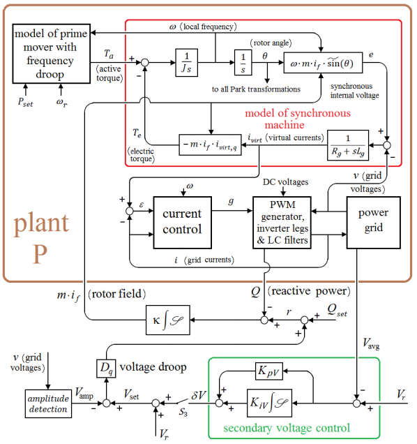
Figure 4: A synchronverter with primary and secondary voltage control loops, based on Fig. 2 from [28] (rearranged). The central secondary voltage control sends the signal $\delta V$ to each synchronverter in the microgrid. $V_{\rm avg}$ is the (weighted) average of several inverter voltage amplitudes.

VI-B Voltage control for an inverter

Here we consider the primary and secondary voltage control loops for a grid-connected synchronverter. For the background on synchronverters (a special type of 3 phase inverters that emulate synchronous machines) we refer to [52, 36, 28], and the references therein. The primary voltage control loop in a synchronverter is meant to react rapidly (on the time scale of tens of milliseconds) to changes in the amplitude $V_{\rm amp}$ of the AC terminal voltages, adjusting the field current $i_{f}$ (and hence the field $mi_{f}$) of the virtual rotor, so that the reactive power $Q$ flowing from the inverter to the grid tracks the expression

$$r{\hbox{\hskip 1.0pt}}={\hbox{\hskip 1.0pt}}Q_{\rm set}+D_{q}(V_{\rm set}-V_{\rm amp}){\hbox{\hskip 1.0pt}}.$$

This means that in steady state, $r-Q$ tends to zero. Here $Q_{\rm set}$ is the set value for the reactive power, $D_{q}$ is the voltage droop coefficient and $V_{\rm set}$ is the desired amplitude of the terminal voltage. This primary voltage control loop can be seen in Fig. 4, the controller (a saturating integrator with gain $\kappa$) is just below the large brown block ${\mathbf{P}}$ that represents the inverter, the power grid and the other blocks of the synchronverter algorithm. The diagram is based in Figure 2 in [28], and we refer the reader to the cited reference for the details of the diagram and the meaning of various variables that appear there, although we have strived to make the picture directly understandable to a reader familiar with inverters.

When several inverters are connected into an islanded microgrid, then it is useful to have a central controller for secondary voltage control. The purpose of the secondary control is to keep the voltages in the microgrid within reasonable bounds, by imposing a certain reference value $V_{r}$ for a weighted average $V_{\rm ave}$ of the terminal voltages amplitudes $V_{\rm amp}$ of the individual inverters. Assuming that the line impedances are low, if in steady state $V_{\rm avg}=V_{r}$, then all the individual terminal voltages will be within reasonable bounds. The secondary voltage controller proposed in [28] is a PI controller with saturating integrator, as discussed in this paper. Its output is a correction $\delta V$ that is added to the voltage reference $V_{r}$ of each inverter. The secondary controller can be seen on the bottom of Fig. 4, and this figure shows clearly that the two controllers are in a nested structure.

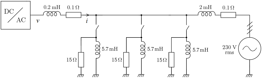
Figure 5: The electric circuit of the system considered in Example VI-B.

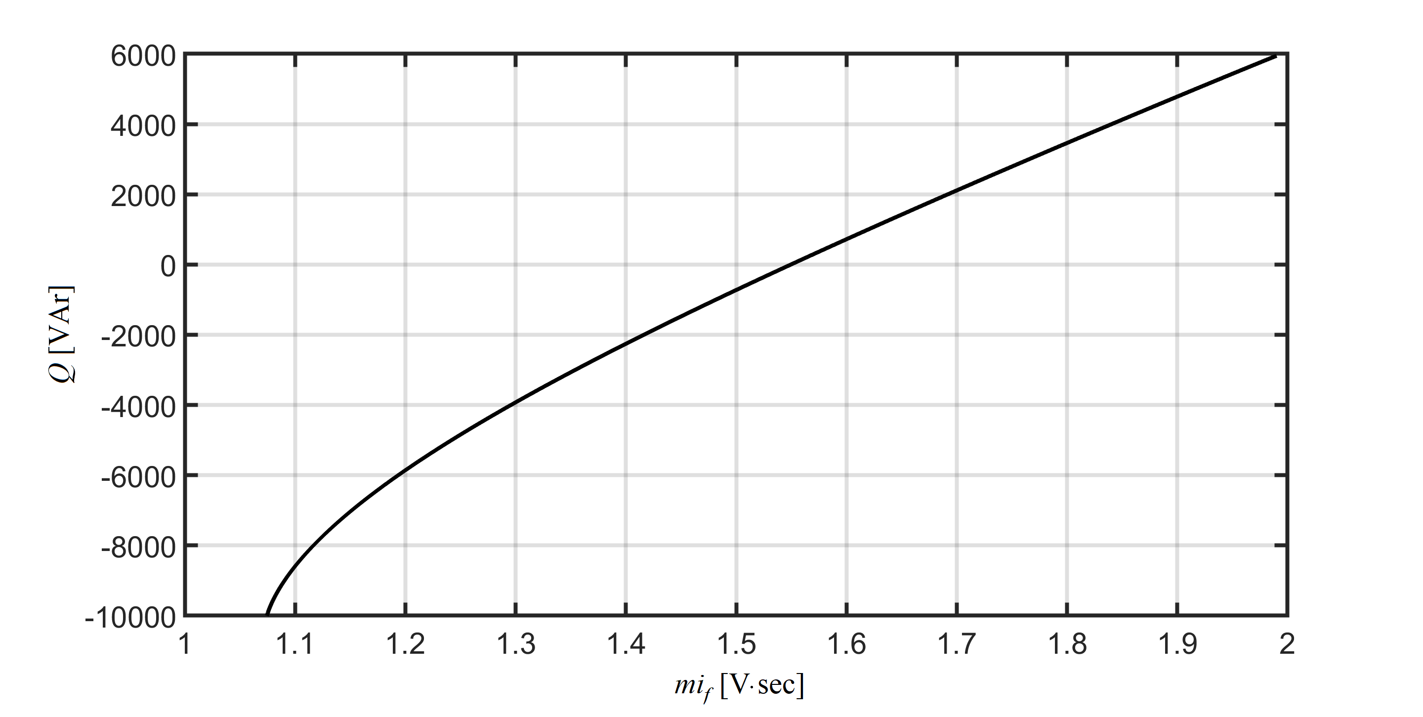
Figure 6: $Q$ as a function of $mi_{f}$, at steady state, for various values of constant $mi_{f}$, in Example VI-B.

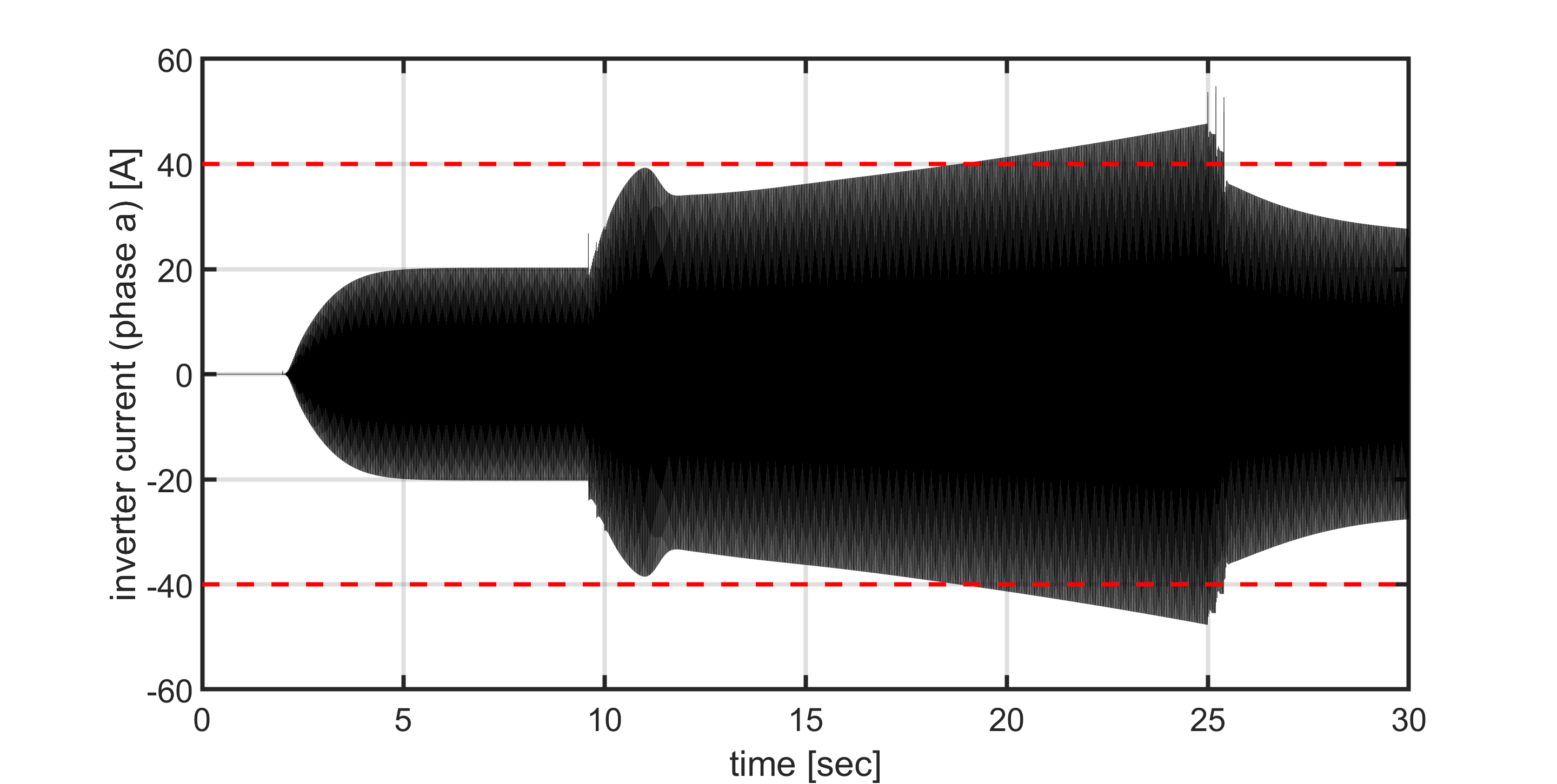
(a) Using classical integrators: After the large load is connected (in three steps) approximately at $t=10$ sec, the current increases beyond the allowed range (marked in dashed red).

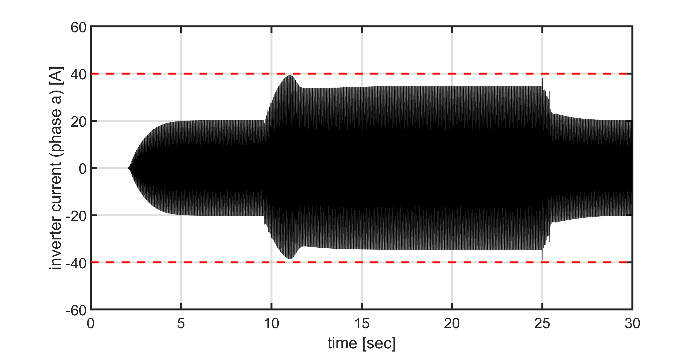
(b) Using saturating integrators: After the large load is connected at $t=10$ sec, the current stablizes quickly to a higher amplitude within the allowed range (marked in dashed red).

Figure 7: Connecting the large consumer causes a voltage drop from about 10 sec to about 25 sec, leading to an increase of the inverter current. The plots show the inverter current in phase a when the I and PI controllers on the bottom of Fig. 4 are without saturation (Subfig. a) and with saturation (Subfig. b).

For our simulation experiment, we have assumed that a single inverter is connected to a power grid representing a large number of other inverters, so that the other inverters together act as an AC voltage source (also called infinite bus), with frequency 50 Hz. There is a line impedance consisting of a 2 mH inductor and a 0.1 $\Omega$ resistor from the inverter to the grid, as shown in Fig. 5. There is a large consumer that connects directly to the inverter for a period of 15 sec, starting at about 10 sec. (The load is split into 3 equal parallel parts to avoid the large current peaks that occur with the connection or disconnection of a large load. These parts act with a delay of 200 msec between them, so that it takes 400 msec to completely connect or to disconnect the load.) During the first 2 sec of the simulations, the synchronverter goes through the start-up procedure and then it connects to the grid. At about $t=5$ sec the grid currents reach steady state, with an amplitude of about 20 A (the nominal current of this inverter), as can be seen in Fig. 7(a) and 7(b). In our simulation experiment, it is assumed that $V_{\rm amp}$ contributes 1/3 of $V_{\rm avg}$, the rest being the infinite bus voltage amplitude, 325.3 V.

For lack of space, we do not provide all the details of the analysis of these control loops. A detailed stability analysis of a closely related but simpler system appears in [32], where the inverter is connected directly to the infinite bus, without all the other circuit elements in Fig. 5, and there is no secondary voltage control ($\delta V=0$ in Fig. 4).

In order for the theory presented here to be applicable to the primary control loop, we need that the plant ${\mathbf{P}}$ should be described by sufficiently smooth functions as in (1), it should be exponentially stable around the equilibrium points corresponding to constant inputs $mi_{f}$ in a certain range $mi_{f}\in[u_{min},u_{max}]$ and in steady state, the dependence of the output $Q$ on $mi_{f}$ (the function $G$ from Assumption 1) should be monotone increasing. The smoothness property is easy to verify if we use the average model for the inverter legs (that are switching at a frequency of several times 10 kHz). The exponential stability for constant $mi_{f}$ is a delicate property that has been proved, under certain sufficient conditions on the parameters, in [2] and in [37] (the conditions that they found are not equivalent). Finally, we have verified the monotone property numerically for a set of typical parameters for a 10 kW synchronverter, the same parameters as used in [28]. We refrain from listing the parameters here, but we show the plot of $Q$ (in steady state) as a function of $mi_{f}$ in Figure 6. A similar plot of monotonicity can be obtained for the secondary control loop (where the input of the new plant is $\delta V$ and its output is $V_{\rm avg}$), but we omit the plot.

During the time when the large load is connected, the terminal voltage of the synchronverter drops considerably, causing the signal $V_{\rm avg}$ to drop as well, so that $\delta V$ starts growing. If the two PI controllers under discussion have normal integrators, then $\delta V$ keeps increasing during the time of low voltage and pushes the signal $mi_{f}$ to increase as well. This increases the synchronous internal voltage $e$, hence the currents, until the currents reach almost 50 A towards the end of the low voltage period, see Fig. 7(a). In reality, this cannot happen, because when the currents reach 40 A (double the nominal current), the protection logic of the inverter disables the gate signals and opens the circuit breaker.

By contrast, if we do the same experiment but using two saturating integrators in the two nested controllers, then the current stabilizes at around 34 A during the low voltage period, and quickly returns to normal steady state after the large consumer is disconnected at around $t=25$ sec, see Fig. 7(b). Notice that the recovery to steady state currents is much quicker in Fig. 7(b) than in Fig. 7(a).

These different behaviors are due to the secondary voltage control integrator state, which, in the case of a classical integrator, tends to windup to excessively large values.

VII Conclusion

We have presented a PI controller with anti-windup (saturating integrator), for a single-input single-output stable nonlinear plant, based on singular perturbations theory. Under reasonable assumptions, we proved that the closed-loop system from Fig. 1 is able to track a constant reference signal $r$, while not allowing the integrator state $u_{I}$ to leave the set $U$. Moreover, the equilibrium point of the closed-loop system is stable and has a “large” region of attraction. If the plant is ISS, then the closed-loop system is globally asymptotically stable. Finally, the validity of our theoretical results has been demonstrated through two examples: a toy example and a real application in the control of a certain type of three phase inverters.

Appendix A Proof of Proposition II.2

For the sake of the proof, we slightly modify the closed-loop system in Fig. 1 by adding a saturation block, using the function $\mathrm{B}_{\eta}$ defined in (35), where $\eta>0$ is fixed, to be determined later. The corresponding modified closed-loop system is shown in Fig. 8, so that $\mathrm{B}_{\eta}$ is applied to $\tau_{p}w$, and it is described by

$$\begin{cases}\begin{gathered}{\hbox{\hskip 1.0pt}}\ \dot{x}{\hbox{\hskip 1.0pt}}={\hbox{\hskip 1.0pt}}f(x,u_{I}+\mathrm{B}_{\eta}(\tau_{p}k(r-g(x)))),\\ \dot{u}_{I}{\hbox{\hskip 1.0pt}}={\hbox{\hskip 1.0pt}}{\mathscr{S}}(u_{I},k(r-g(x))).\end{gathered}\end{cases}$$ (40)

Notation. For any $R>0$, $B_{R}$ is the closed ball of radius $R$ in $\mathbb{R}^{n}$. For any $\tau>0$ we denote by $C_{\tau}$ the set of all the continuous functions on the interval $[0,\tau]$, with values in $U_{\eta}\vcentcolon=[u_{min}-\eta,u_{max}+\eta]$. This is a complete metric space with the distance induced by the supremum norm $\lVert\cdot\rVert_{\infty}$.

Lemma A.1

Take $x_{0}\in{\mathbb{R}}^{n}$ and $R>0$. Denote $M=\max\{\|f(x,v)\|\ |\ x\in x_{0}+B_{R},\ v\in U_{\eta}\}$ and let $\tau\in(0,R/M]$. Then, for every $u\in C_{\tau}$, (1) has a unique solution $x\in C^{1}([0,\tau];{\mathbb{R}}^{n})$ and $x(t)\in x_{0}+B_{R}$ for all $t\in[0,\tau]$.

The (nonlinear) operator $T_{\tau}$ determined by ${\mathbf{P}}$, that maps any input function $u\in C_{\tau}$ into an output function $y\in C[0,\tau]$ (corresponding to $x(0)=x_{0}$) is Lipschitz continuous, with Lipschitz constant of the form $\tau L_{T}$, where $L_{T}>0$ is independent of $\tau$.

Proof:

It follows from classical ODE theory and the mean value theorem that for any $u\in C_{\tau}$, the state trajectory $x(t)$ of ${\mathbf{P}}$ exists and remains in $x_{0}+B_{R}$ for all $t\leq\tau$. Let $L_{1},L_{2}>0$ be such that for any $z_{1},z_{2}\in x_{0}+B_{R}$, and for any $v_{1},v_{2}\in U_{\eta}$

$$\|f(z_{2},v_{2})-f(z_{1},v_{1})\|{\hbox{\hskip 1.0pt}}\leq{\hbox{\hskip 1.0pt}}L_{1}\|z_{2}-z_{1}\|+L_{2}\|v_{2}-v_{1}\|.$$ (41)

Such $L_{1},L_{2}$ exist since $f\in C^{2}$ and $\{x_{0}+B_{R}\}\times U_{\eta}$ is compact. Take two state trajectories of ${\mathbf{P}}$, $x_{1}$ and $x_{2}$, starting from the same initial state $x_{0}$ and corresponding to inputs $u_{1}$ and $u_{2}$. Then

$$x_{2}(t)-x_{1}(t)=\int_{0}^{t}\big{[}f(x_{2}(\sigma),u_{2}(\sigma))-f(x_{1}(\sigma),u_{1}(\sigma))\big{]}{\rm d}\hbox{\hskip 0.5pt}\sigma,$$

for any $t\in[0,\tau]$, whence, using (41),

$$\lVert x_{2}(t)-x_{1}(t)\rVert\leq L_{1}\int_{0}^{t}\lVert x_{2}(\sigma)-x_{1}(\sigma)\rVert{\rm d}\hbox{\hskip 0.5pt}\sigma+\tau L_{2}\lVert u_{2}-u_{1}\rVert_{\infty}.$$

It follows from Gronwall’s inequality that

$$\lVert x_{2}(t)-x_{1}(t)\rVert\leq\tau L_{2}\lVert u_{1}-u_{2}\rVert_{\infty}\;e^{L_{1}t}{\hbox{$\hskip 31.29802pt\forall\;$}}t\in[0,\tau],$$

which implies that

$$\|x_{2}-x_{1}\|_{\infty}{\hbox{\hskip 1.0pt}}\leq{\hbox{\hskip 1.0pt}}\tau L_{2}\|u_{1}-u_{2}\|_{\infty}\;e^{L_{1}\tau}.$$

Finally, since $g\in C^{1}$, we get

$$\|y_{2}-y_{1}\|_{\infty}{\hbox{\hskip 1.0pt}}\leq{\hbox{\hskip 1.0pt}}\tau L_{T}^{\tau}\|u_{1}-u_{2}\|_{\infty},$$

where $L_{T}^{\tau}=L_{2}e^{L_{1}\tau}L_{g}$ and $L_{g}$ is the Lipschitz constant of $g$ on the set $x_{0}+B_{R}$. Taking the largest possible value for $\tau$, i.e., $\tau=\frac{R}{M}$, we get $L_{T}=L_{2}e^{L_{1}\frac{R}{M}}L_{g}$. ∎

Figure 8: The modified closed-loop system formed by the plant ${\mathbf{P}}$, the saturating integrator $\int{\mathscr{S}}$, the constant gains $k>0$, $\tau_{p}\geq 0$ and the saturation function $\mathrm{B}_{\eta}$, with the reference signal $r$.

Proof of Proposition II.2: We use the notation from Lemma A.1, in particular, $R>0$ is arbitrary and $x_{0}$, $u_{0}$ are fixed. As we have shown in the previous lemma, the Lipschitz bound of $T_{\tau}$ is $\tau L_{T}$, where $L_{T}>0$ is independent of $\tau\in(0,R/M]$. We choose $\eta>\delta$ large enough such that $\lvert\tau_{p}ke(0)\rvert<\eta$, where $e(0)=r-g(x_{0})$. Let us denote by $S_{\tau}$ the input to output map of the saturating integrator on the time interval $[0,\tau]$, corresponding to $u_{I}(0)=u_{0}$, and let $\mathrm{B}_{\eta}$ denote the (Lipschitz continuous) operator on $C[0,\tau]$ obtained from the function $\mathrm{B}_{\eta}$ by applying it pointwise. The estimate (6) shows that $S_{\tau}:C[0,\tau]\mapsto C_{\tau}$ is Lipschitz continuous with Lipschitz constant $\tau$. If $(x,u_{I})$ is a state trajectory of the modified closed-loop system which is defined on $[0,\tau]$, and we define $e=r-g(x)$, then we must have (see Fig. 8)

$$e{\hbox{\hskip 1.0pt}}={\hbox{\hskip 1.0pt}}r-T_{\tau}(S_{\tau}+\mathrm{B}_{\eta}\tau_{p})k{\hbox{\hskip 1.0pt}}e.$$

This can be regarded as a fixed point equation on $C[0,\tau]$. For $\tau$ sufficiently small so that $\tau L_{T}\cdot(\tau+\lvert\tau_{p}\rvert)\cdot\lvert k\rvert<1$, the above equation has a unique solution $e$ according to the Banach fixed point theorem, see for instance [4, Sect. 3]. It is easy to see that if $e$ is a solution of the fixed point equation, if $u=(S_{\tau}+\mathrm{B}_{\eta}\tau_{p})ke$, $x$ is the corresponding state trajectory of ${\mathbf{P}}$ starting from $x_{0}$, and $u_{I}=S_{\tau}ke$, then $(x,u_{I})$ is the desired unique state trajectory of (40) on $[0,\tau]$.

To extend the above result to the closed-loop system shown in Fig. 1, recall from the beginning of the proof that $\lvert\tau_{p}ke(0)\rvert<\eta$, i.e., the saturation function $\mathrm{B}_{\eta}$ from Fig. 8 is not saturated at $t=0$. Since $e(t)=r-g(x(t))$ is a continuous function, there exists $\tau^{\prime}\in(0,\tau]$ such that $\lvert\tau_{p}ke(t)\rvert<\eta$ remains true for $t\in[0,\tau^{\prime})$. Then, on the time interval $[0,\tau^{\prime})$ the equations satisfied by $(x,u_{I})$ are precisely (4). Hence, $(x,u_{I})$ is the unique solution of (4) on $[0,\tau^{\prime})$. This $\tau^{\prime}$ is what we have called $\tau$ in the proposition.

Finally, using standard arguments, see for instance Exercise 3.26 in [24], we get that if an interval of existence $[0,\tau)$ is such that $\tau>0$ is finite and maximal, then $\limsup_{t\mathop{\rightarrow}\tau}\|(x(t),u_{I}(t))\|=\infty$, implying that $\limsup_{t\mathop{\rightarrow}\tau}\|x(t)\|=\infty$. ∎

Remark A.2

An alternative way to prove existence (but not uniqueness) of the solution to the closed-loop system (4) is to use tools from differential inclusions theory. In particular, (2) can be regarded as a constrained differential inclusion, see for example (5.4) in [11], where the state $u$ is constrained in the closed set $U$ and the map ${\mathscr{S}}$ is replaced with the Krasovskii set-valued map

$$\begin{gathered}{\mathscr{S}}_{K}(u_{I},w){\hbox{\hskip 1.0pt}}={\hbox{\hskip 1.0pt}}\begin{cases}\{w^{+}\}&\text{if}\quad u_{I}<u_{min},\\ [w,w^{+}]&\text{if}\quad u_{I}=u_{min},\\ \{w\}&\text{if}\quad u_{I}\in(u_{min},u_{max}),\\ [w^{-},w]&\text{if}\quad u_{I}=u_{max},\\ \{w^{-}\}&\text{if}\quad u_{I}>u_{max}.\end{cases}\end{gathered}$$

The set-valued map describing the closed-loop system is outer semicontinuous (see Definition 5.9 of [11]). Therefore, the closed-loop system (4) satisfies Assumption 6.5 of [11] and, according to Theorem 6.30 of [11], it is well-posed.

Appendix B Proof of Theorem IV.2

By assumption, there exist two Lyapunov functions $V$ and $W$, for the reduced system (22) and for the boundary-layer system (24), respectively, so that the conditions presented in the first 12 lines of the proof of Theorem 11.4 in [24] hold (our (25), (27)). The translation between our notation and the one in [24] is, again, given by Table I. (Note that, unlike in Theorem 11.4 of [24], assuming that the origin of (22) is exponentially stable is not enough in our case to apply the converse Theorem 4.14 from [24], since $\tilde{h}\notin C^{1}$.) If we define $z$ as in (19), then equations (11.49)-(11.50) in [24] translate to our (20)-(21).

We prove some estimates. Since the system (20)-(21) is time-invariant and $\tilde{h}$ is independent of $k$, the growth conditions (valid in a neighbourhood of the origin) shown in [24] (after (11.50)) reduce in our case to

$$\big{\|}\tilde{\beta}(\tilde{u}_{I},z+\tilde{\Xi}(\tilde{u}_{I}),k)\big{\|}\leq k\alpha_{1}(|\tilde{u}_{I}|+\lVert z\rVert),$$ (42a)

$$\big{|}\tilde{h}(\tilde{u}_{I},z+\tilde{\Xi}(\tilde{u}_{I}))-\tilde{h}(\tilde{u}_{I},\tilde{\Xi}(\tilde{u}_{I}))\big{|}\leq\alpha_{2}\lVert z\rVert,$$ (42b)

$$\big{|}\tilde{h}(\tilde{u}_{I},\tilde{\Xi}(\tilde{u}_{I}))\big{|}\leq\alpha_{3}|\tilde{u}_{I}|,\quad\bigg{\|}\frac{{\rm d}\hbox{\hskip 0.5pt}\tilde{\Xi}}{{\rm d}\hbox{\hskip 0.5pt}\tilde{u}_{I}}\bigg{\|}\leq\alpha_{4},$$ (42c)

where $\alpha_{1},\dots\alpha_{4}$ are positive constants. These estimates follow respectively from:

• $\tilde{\beta}\in{\rm Lip}$ and $\tilde{\beta}(\tilde{u}_{I},\tilde{x},0)=0$ for all $(\tilde{u}_{I},\tilde{x})\in\tilde{X}_{\delta}$,

• $\tilde{h}$ being uniformly Lipschitz in the second argument,

• $\tilde{h}$ being uniformly Lipschitz in the second argument, $\tilde{\Xi}\in C^{1}$, $\tilde{h}(0,0)=0$, and $\tilde{\Xi}(0)=0$.

• $\tilde{\Xi}\in C^{1}$.

Consider the function $\nu$ from (29) as a Lyapunov function candidate for the system (20)-(21). Computing its derivative along the state trajectories of (20)-(21), we get

$$\frac{{\rm d}\hbox{\hskip 0.5pt}\nu}{{\rm d}\hbox{\hskip 0.5pt}s}=\frac{{\rm d}\hbox{\hskip 0.5pt}V}{{\rm d}\hbox{\hskip 0.5pt}\tilde{u}_{I}}\frac{{\rm d}\hbox{\hskip 0.5pt}\tilde{u}_{I}}{{\rm d}\hbox{\hskip 0.5pt}s}+\frac{\partial W}{\partial\tilde{u}_{I}}\frac{{\rm d}\hbox{\hskip 0.5pt}\tilde{u}_{I}}{{\rm d}\hbox{\hskip 0.5pt}s}+\frac{\partial W}{\partial z}\frac{{\rm d}\hbox{\hskip 0.5pt}z}{{\rm d}\hbox{\hskip 0.5pt}s}.$$ (43)

Consider the first term on the right-hand side of (43). Substituting (20) we obtain

$$\frac{{\rm d}\hbox{\hskip 0.5pt}V}{{\rm d}\hbox{\hskip 0.5pt}\tilde{u}_{I}}\tilde{h}(\tilde{u}_{I},z+\tilde{\Xi}(\tilde{u}_{I}))\leq\frac{{\rm d}\hbox{\hskip 0.5pt}V}{{\rm d}\hbox{\hskip 0.5pt}\tilde{u}_{I}}\tilde{h}(\tilde{u}_{I},\tilde{\Xi}(\tilde{u}_{I}))\\ +\bigg{|}\frac{{\rm d}\hbox{\hskip 0.5pt}V}{{\rm d}\hbox{\hskip 0.5pt}\tilde{u}_{I}}\bigg{|}\big{|}\tilde{h}(\tilde{u}_{I},z+\tilde{\Xi}(\tilde{u}_{I}))-\tilde{h}(\tilde{u}_{I},\tilde{\Xi}(\tilde{u}_{I}))\big{|}.$$

Using (25) and (42b), we have

$$\frac{{\rm d}\hbox{\hskip 0.5pt}V}{{\rm d}\hbox{\hskip 0.5pt}\tilde{u}_{I}}\frac{{\rm d}\hbox{\hskip 0.5pt}\tilde{u}_{I}}{{\rm d}\hbox{\hskip 0.5pt}s}\leq-c_{3}\lvert\tilde{u}_{I}\rvert^{2}+\alpha_{2}c_{4}\lvert\tilde{u}_{I}\rvert\lVert z\rVert.$$ (44)

Consider the second term on the right-hand side of (43). Substituting (20) we obtain

$$\frac{\partial W}{\partial\tilde{u}_{I}}\tilde{h}(\tilde{u}_{I},z+\tilde{\Xi}(\tilde{u}_{I}))\leq\bigg{\|}\frac{\partial W}{\partial\tilde{u}_{I}}\bigg{\|}\bigg{[}\big{|}\tilde{h}(\tilde{u}_{I},\tilde{\Xi}(\tilde{u}_{I}))\big{|}\\ +\big{|}\tilde{h}(\tilde{u}_{I},z+\tilde{\Xi}(\tilde{u}_{I}))-\tilde{h}(\tilde{u}_{I},\tilde{\Xi}(\tilde{u}_{I}))\big{|}\bigg{]}.$$

Using (27), (42b) and (42c), we get

$$\frac{\partial W}{\partial\tilde{u}_{I}}\frac{{\rm d}\hbox{\hskip 0.5pt}\tilde{u}_{I}}{{\rm d}\hbox{\hskip 0.5pt}s}\leq b_{5}\lVert z\rVert^{2}\big{(}\alpha_{2}\lVert z\rVert+\alpha_{3}|\tilde{u}_{I}|\big{)}.$$ (45)

Finally, consider the third term on the right-hand side of (43). Substituting (21) we obtain

$$\frac{\partial W}{\partial z}\bigg{[}\frac{1}{k}\tilde{f}(\tilde{u}_{I},z+\tilde{\Xi}(\tilde{u}_{I}))+\frac{1}{k}\tilde{\beta}(\tilde{u}_{I},z+\tilde{\Xi}(\tilde{u}_{I}),k)\\ -\frac{{\rm d}\hbox{\hskip 0.5pt}\tilde{\Xi}}{{\rm d}\hbox{\hskip 0.5pt}\tilde{u}_{I}}\tilde{h}(\tilde{u}_{I},z+\tilde{\Xi}(\tilde{u}_{I}))\bigg{]}$$

$$\leq\frac{1}{k}\frac{\partial W}{\partial z}\tilde{f}(\tilde{u}_{I},z+\tilde{\Xi}(\tilde{u}_{I}))+\bigg{\|}\frac{\partial W}{\partial z}\bigg{\|}\bigg{[}\frac{1}{k}\big{\|}\tilde{\beta}(\tilde{u}_{I},z+\tilde{\Xi}(\tilde{u}_{I}),k)\|\\ +\bigg{\|}\frac{{\rm d}\hbox{\hskip 0.5pt}\tilde{\Xi}}{{\rm d}\hbox{\hskip 0.5pt}\tilde{u}_{I}}\bigg{\|}\big{\|}\tilde{h}(\tilde{u}_{I},z+\tilde{\Xi}(\tilde{u}_{I}))\big{\|}\bigg{]}.$$

Proceeding as before and using (27), (42), we get

$$\frac{\partial W}{\partial z}\frac{{\rm d}\hbox{\hskip 0.5pt}z}{{\rm d}\hbox{\hskip 0.5pt}s}\leq-\frac{b_{3}}{k}\lVert z\rVert^{2}+\alpha_{1}b_{4}\lVert z\rVert(\lvert\tilde{u}_{I}\rvert+\lVert z\rVert)\\ +\alpha_{4}b_{4}\lVert z\rVert(\alpha_{2}\lVert z\rVert+\alpha_{3}\lvert\tilde{u}_{I}\rvert).$$ (46)

Putting together (44), (45) and (46), we have from (43)

$$\frac{{\rm d}\hbox{\hskip 0.5pt}\nu}{{\rm d}\hbox{\hskip 0.5pt}s}\leq-c_{3}\lvert\tilde{u}_{I}\rvert^{2}-\frac{b_{3}}{k}\lVert z\rVert^{2}+d_{1}\lVert z\rVert^{2}\\ +d_{2}\lvert\tilde{u}_{I}\rvert\lVert z\rVert+d_{3}\lvert\tilde{u}_{I}\rvert\lVert z\rVert^{2}+d_{4}\lVert z\rVert^{3},$$

with positive $c_{3}$, $b_{3}$ and non negative $d_{1},\dots d_{4}$. For all $z\leq{\varepsilon}_{0}$, this reduces to

$$\frac{{\rm d}\hbox{\hskip 0.5pt}\nu}{{\rm d}\hbox{\hskip 0.5pt}s}\leq-c_{3}\lvert\tilde{u}_{I}\rvert^{2}-\frac{b_{3}}{k}\lVert z\rVert^{2}+d_{5}\lVert z\rVert^{2}+2d_{6}\lvert\tilde{u}_{I}\rvert\lVert z\rVert,$$

for non negative $d_{5}$, $d_{6}$. The above inequality can be rewritten in matrix form as

$$\frac{{\rm d}\hbox{\hskip 0.5pt}\nu}{{\rm d}\hbox{\hskip 0.5pt}s}\leq-\begin{bmatrix}\lvert\tilde{u}_{I}\rvert\\ \lVert z\rVert\\ \end{bmatrix}^{T}\begin{bmatrix}c_{3}&-d_{6}\\ -d_{6}&\frac{b_{3}}{k}-d_{5}\end{bmatrix}\begin{bmatrix}\lvert\tilde{u}_{I}\rvert\\ \lVert z\rVert\\ \end{bmatrix}.$$

(Note that, differently from [24], $k$ does not appear in the upper-left term, since our reduced model (22) is independent of $k$.) Therefore, there exists a $\kappa>0$ such that for all $0<k<\kappa$, we have $\frac{{\rm d}\hbox{\hskip 0.5pt}\nu}{{\rm d}\hbox{\hskip 0.5pt}s}\leq-2\gamma\nu$, for some $\gamma>0$. It follows that

$$\nu(\tilde{u}_{I}(s),z(s))\leq e^{-\gamma s}\nu(\tilde{u}_{I}(0),z(0)),$$

and from (25), (27)

$$\begin{bmatrix}\lvert\tilde{u}_{I}(s)\rvert\\ \lVert z(s)\rVert\\ \end{bmatrix}\leq K_{1}e^{-\gamma s}\begin{bmatrix}\lvert\tilde{u}_{I}(0)\rvert\\ \lVert z(0)\rVert\\ \end{bmatrix},$$ (47)

for some $K_{1}>0$. Recall the change of variables (19), since $\lVert\tilde{\Xi}(\tilde{u}_{I})\rVert\leq L_{\tilde{\Xi}}\lvert\tilde{u}_{I}\rvert$ ($\tilde{\Xi}\in C^{2}$ and $\tilde{U}_{\delta}$ compact), then from (47) it follows that

$$\begin{bmatrix}\lvert\tilde{u}_{I}(s)\rvert\\ \lVert\tilde{x}(s)\rVert\\ \end{bmatrix}\leq K_{2}e^{-\gamma s}\begin{bmatrix}\lvert\tilde{u}_{I}(0)\rvert\\ \lVert\tilde{x}(0)\rVert\\ \end{bmatrix},$$

for some $K_{2}>0$, completing the proof. ∎

Appendix C Proof of Proposition V.2

As assumed in the proposition, $g$ is bounded or $\tau_{p}=0$. Choose an initial state $(x_{0},u_{0})\in X_{\delta}$ for the closed-loop system (4). From Proposition II.2 it follows that there exists a maximal $\tau\in(0,\infty]$ such that (4) has a unique state trajectory $(x,u_{I})$ defined on $[0,\tau)$. If $\tau$ is finite, then $\limsup_{t\mathop{\rightarrow}\tau}\|x(t)\|=\infty$. This contradicts Proposition V.1. Indeed, recalling the definition of $\int\mathscr{S}$ from (2), $u_{I}(t)\in U_{\delta}$ for all $t\geq 0$. Thus, according to Proposition V.1, $\lVert x(t)\rVert$ is bounded for all $t\geq 0$. Therefore, for any $(x_{0},u_{0})\in X_{\delta}$, (4) has a unique global solution for all $k>0$ and $r\in Y$.

We now prove continuous dependence of the solution on the initial state. Take $(x_{0},u_{0})$ and $(\bar{x}_{0},\bar{u}_{0})$ to be initial states in $X_{\delta}$. Let $(x,u_{I})$ be the state trajectory of (4) for the initial state $(x_{0},u_{0})$, and, similarly, let $(\bar{x},\bar{u}_{I})$ be the state trajectory corresponding to $(\bar{x}_{0},\bar{u}_{0})$. Denote by $B_{R}$ the closed ball of radius $R$ in $\mathbb{R}^{n}$. Let $M>0$ be such that $\lvert u(t)-v\rvert\leq M$ for all $t\geq 0$, for any trajectory of (4) starting in $X_{\delta}$, and for any $v\in U_{\delta}$. Such an $M$ exists because $g$ is bounded or $\tau_{p}=0$. Then from (33) we have, for any $v\in U_{\delta}$,

$$\lVert x(t)-\Xi(v)\rVert\leq\alpha_{v}(\lVert x_{0}-\Xi(v)\rVert,t)+\gamma(M),$$

$$\lVert\bar{x}(t)-\Xi(v)\rVert\leq\alpha_{v}(\lVert\bar{x}_{0}-\Xi(v)\rVert,t)+\gamma(M),$$

which implies that there exists $\rho>0$ such that $x(t),\bar{x}(t)\in B_{\rho}$ for all $t\geq 0$. Let $L_{1},L_{2}>0$ be such that

$$\lVert f(z_{2},v_{2})-f(z_{1},v_{1})\rVert{\hbox{\hskip 1.0pt}}\leq{\hbox{\hskip 1.0pt}}L_{1}\lVert z_{2}-z_{1}\rVert+L_{2}\lvert v_{2}-v_{1}\rvert,$$

for any $z_{1},z_{2}\in B_{\rho}$ and for any $v_{1},v_{2}\in U_{\delta}$. Such $L_{1},L_{2}$ exist since $f\in C^{2}$ and $B_{\rho}\times U_{\delta}$ is compact. It follows that

$$\lVert x(t)-\bar{x}(t)\rVert\leq\lVert x_{0}-\bar{x}_{0}\rVert+L_{1}\int_{0}^{t}\lVert x(\sigma)-\bar{x}(\sigma)\rVert{\rm d}\hbox{\hskip 0.5pt}\sigma\\ +L_{2}\int_{0}^{t}\lvert u_{I}(\sigma)-\bar{u}_{I}(\sigma)\rvert{\rm d}\hbox{\hskip 0.5pt}\sigma.$$ (48)

Besides, from (5) (extended to continuous functions) we have

$$\lvert u_{I}(t)-\bar{u}_{I}(t)\rvert{\hbox{\hskip 1.0pt}}\leq{\hbox{\hskip 1.0pt}}\lvert u_{I}(0)-\bar{u}_{I}(0)\rvert+\int_{0}^{t}\lvert w(\sigma)-\bar{w}(\sigma)\rvert{\rm d}\hbox{\hskip 0.5pt}\sigma,$$

where $w(\sigma)=k(r-g(x(\sigma)))$, $\bar{w}(\sigma)=k(r-g(\bar{x}(\sigma)))$. Let $L_{3}$ be the Lipschitz constant of $g$ on $B_{\rho}$, then

$$\lvert w(\sigma)-\bar{w}(\sigma)\rvert{\hbox{\hskip 1.0pt}}\leq{\hbox{\hskip 1.0pt}}kL_{3}\lVert x(\sigma)-\bar{x}(\sigma)\rVert,$$ (49)

for all $\sigma\geq 0$ and $x,\bar{x}\in B_{\rho}$. Adding (48) to (49), we get

$$\lVert x(t)-\bar{x}(t)\rVert+\lvert u_{I}(t)-\bar{u}_{I}(t)\rvert\leq\lVert x_{0}-\bar{x}_{0}\rVert+\lvert u_{0}-\bar{u}_{0}\rvert\\ +(L_{1}+kL_{3})\int_{0}^{t}\lVert x(\sigma)-\bar{x}(\sigma)\rVert{\rm d}\hbox{\hskip 0.5pt}\sigma+L_{2}\int_{0}^{t}\lvert u_{I}(\sigma)-\bar{u}_{I}(\sigma)\rvert{\rm d}\hbox{\hskip 0.5pt}\sigma.$$

Denote $L_{4}=\max\{L_{1}+kL_{3},L_{2}\}$, then defining $q(t)\vcentcolon=\lVert x(t)-\bar{x}(t)\rVert+\lvert u_{I}(t)-\bar{u}_{I}(t)\rvert$, the last estimate becomes

$$q(t){\hbox{\hskip 1.0pt}}\leq{\hbox{\hskip 1.0pt}}q(0)+L_{4}\int_{0}^{t}q(\sigma){\rm d}\hbox{\hskip 0.5pt}\sigma.$$

Finally, using the Gronwall inequality, we get

$$q(t){\hbox{\hskip 1.0pt}}\leq{\hbox{\hskip 1.0pt}}q(0)e^{L_{4}t}.$$

This shows that at any $t\geq 0$, the state $(x(t),u_{I}(t))$ from (4) depends Lipschitz continuously on the initial state $(x_{0},u_{0})$. ∎

Appendix D Proof of Theorem V.3

Lemma D.1

We work under the assumptions of Proposition V.2. Let $T>0$ and let $X_{T}\subset X_{\delta}$ be a compact set such that if $(x_{0},u_{0})\in X_{T}$, then the state trajectory $x$ of ${\mathbf{P}}$ starting from $x(0)=x_{0}$, with constant input $u_{0}$, satisfies

$$\lVert x(T)-\Xi(u_{0})\rVert{\hbox{\hskip 1.0pt}}\leq{\hbox{\hskip 1.0pt}}{\varepsilon}_{0}{\hbox{\hskip 1.0pt}}.$$

Then there exists a $\kappa_{T}>0$ such that for any $k\in(0,\kappa_{T})$, for any $r\in Y$, if the initial state $(x_{0},u_{0})$ of (4) is in $X_{T}$, then its state trajectory $(x,u_{I})$ satisfies

$$x(t)\mathop{\rightarrow}\Xi(u_{r}),\qquad u(t)\mathop{\rightarrow}u_{r},\qquad y(t)\mathop{\rightarrow}r,$$ (50)

and this convergence is at an exponential rate.

Proof:

Take $r\in Y$. Recall the changes of variables (15), (19) and the state space $\tilde{X}_{\delta}=\tilde{U}_{\delta}\times{\mathbb{R}}^{n}$ of the closed-loop system (20)-(21). Define the set $\tilde{X}_{T}\subset\tilde{X}_{\delta}$ as the image of the set $X_{T}$ through the change of variables just mentioned. Then for any $(\tilde{u}_{0},z_{0})\in\tilde{X}_{T}$, the state trajectory $z$ of the boundary-layer system (24) starting from $z(0)=z_{0}$, with fixed input $\tilde{u}_{0}$, satisfies $\lVert z(T)\rVert\leq{\varepsilon}_{0}$. Clearly $\tilde{X}_{T}$ is compact.

The convergence of $z$ to $0$ can be regarded as an exponential one. Indeed, for $\lVert z_{0}\rVert\leq{\varepsilon}_{0}$ this is clear from (8). For $\lVert z_{0}\rVert>{\varepsilon}_{0}$ we invoke a compactness argument: there exist $\tilde{m}>0$ such that $\lVert z(t)\rVert\leq\tilde{m}e^{-{\lambda}t}\lVert z_{0}\rVert$ for all $(z_{0},\tilde{u}_{0})\in\tilde{X}_{T}$ with $\lVert z_{0}\rVert\geq{\varepsilon}_{0}$ and for all $t\in[0,T]$. Then for $t>T$ we have, according to (8), $\lVert z(t)\rVert\leq\tilde{m}e^{-{\lambda}(t-T)}\lVert z(T)\rVert\leq\tilde{m}me^{-{\lambda}t}\lVert z_{0}\rVert$.

Applying Lemma 9.8 of [24], we get a Lyapunov function $W(\tilde{u}_{I},z)$ for the boundary-layer system (24) such that (27) holds for all $(\tilde{u}_{I},z)\in\tilde{X}_{T}$. The constants $b_{i}$, $i=1,\dots 5$ from (27) in this case are different, since $\tilde{m}_{T}$ and $\tilde{{\lambda}}_{T}$ are, in general, different from $m$ and ${\lambda}$ of Assumption 1. From this point on, we apply Theorem IV.2 and everything proceeds as in the proof of Theorem IV.3, substituting the inequality (30) with

$$W(\tilde{u}_{I},z)\leq b_{2}\max\{\lVert z\rVert^{2}\ |\ z\in\Pi\tilde{X}_{T}\}\ \ \ \forall{\hbox{\hskip 1.0pt}}(\tilde{u}_{I},z)\in\tilde{X}_{T},$$ (51)

where $\Pi$ denotes the projection onto the second component in the product $\tilde{U}_{\delta}\times{\mathbb{R}}^{n}$, and modifying the definition of $L$ in (31) by substituting $b_{2}{\varepsilon}_{0}^{2}$ with the right-hand side of (51). ∎

Proof of Theorem V.3: For any $(x_{0},u_{0})\in X$, we denote by $\phi(t,x_{0},u_{0})$ the solution of (1) corresponding to the initial state $x_{0}$ and the constant input $u_{0}$. Then Assumption 1 implies that for $\lVert z_{0}\rVert\leq{\varepsilon}_{0}$ we have

$$\lVert\phi(t,x_{0},u_{0})-\Xi(u_{0})\rVert\leq me^{-{\lambda}t}\lVert x_{0}-\Xi(u_{0})\rVert,$$

for all $t\geq 0$. For each $T>0$, we define the relatively open set $\mathring{X}_{T}\subset X$ as follows:

$$\mathring{X}_{T}{\hbox{\hskip-3.0pt}}{\hbox{\hskip 1.0pt}}=\{(x_{0},u_{0}){\hbox{\hskip-3.0pt}}{\hbox{\hskip 0.5pt}}\in{\hbox{\hskip-3.0pt}}{\hbox{\hskip 1.0pt}}X{\hbox{\hskip 1.0pt}}|\ \lVert\phi(T,x_{0},u_{0})-\Xi(u_{0})\rVert{\hbox{\hskip-3.0pt}}<{\hbox{\hskip-3.0pt}}{\hbox{\hskip 0.5pt}}{\varepsilon}_{0},{\hbox{\hskip 0.5pt}}\lVert x_{0}\rVert{\hbox{\hskip-3.0pt}}{\hbox{\hskip 0.5pt}}<{\hbox{\hskip-3.0pt}}{\hbox{\hskip 0.5pt}}T\}.$$

Clearly Assumption 3 implies that every $(x_{0},u_{0})\in X$ is contained in some of the sets $\mathring{X}_{T}$. In other words, the union of all the sets $\mathring{X}_{T}$ is $X$.

Let us choose an (arbitrary) upper bound $k_{max}>0$ for the gain $k$ in Fig. 1. It follows from the assumptions that there exists an $M>0$ such that for any state trajectory $(x,u_{I})$ of (4) (with any $r\in Y$, any gain $k\in[0,k_{max}]$ and starting from any initial state in $X$), the function $u=u_{I}+\tau_{p}k(r-g(x))$ satisfies $|u(t)|\leq M$. Denote $R=\gamma(M)+1+\max_{u_{0}\in U}\lVert\Xi(u_{0})\rVert$ and, as usual, $B_{R}$ is the closed ball of radius $R$ in ${\mathbb{R}}^{n}$. We claim that for any $r\in Y$, any $k\in[0,k_{max}]$ and for any initial state $(x_{0},u_{0})\in X$, the closed-loop system (4) has a solution for all $t\geq 0$ and there exists $T^{*}>0$ such that $x(t)\in B_{R}$, for all $t\geq T^{*}$. Indeed, if we choose $T^{*}>0$ such that $\alpha_{u_{0}}(\lVert x_{0}-\Xi(u_{0})\rVert,T^{*})\leq 1$, then from (33),

$$\lVert x(t)-\Xi(u_{0})\rVert{\hbox{\hskip 1.0pt}}\leq{\hbox{\hskip 1.0pt}}1+\gamma(M){\hbox{$\hskip 31.29802pt\forall\;$}}{\hbox{\hskip 1.0pt}}t\geq T^{*},$$

which implies our previous claim. Since $B_{R}$ is compact and the sets {$\mathring{X}_{T}\ |\ T>0$} are an open covering of $B_{R}$, we can extract a finite cover. Since $\mathring{X}_{T}$ is increasing with $T$, there exists $T>0$ such that $B_{R}\subset\mathring{X}_{T}$. Let us denote by $X_{T}$ the closure of $\mathring{X}_{T}$. Then we can apply Lemma D.1 for this $X_{T}$, to conclude that there exists $\kappa^{*}\in(0,k_{max}]$ such that for any $k\in(0,\kappa^{*}]$, every state trajectory of (4) that, at some point, is in $X_{T}$ satisfies (50) and the convergence is at an exponential rate. But we have seen earlier that every state trajectory of (4) (starting from any initial state) reaches $B_{R}$ in some time. Hence (since $B_{R}\subset X_{T}$), we conclude that for any $k\in(0,\kappa^{*}]$, any state trajectory of (4) satisfies (50) and the convergence is at an exponential rate. ∎

Pietro Lorenzetti is an Early Stage Researcher within the Marie Curie ITN project “ConFlex”, who focuses his research on nonlinear control. He is working under the supervision of George Weiss, and his co-supervisor is Enrique Zuazua. Pietro has completed the bachelor degree in “Computer engineering and automation” at Universita Politecnica delle Marche, in Ancona. In 2015 he graduated with honours and he moved to Torino, where he enrolled the master degree in “Mechatronic Engineering” at Politecnico di Torino. In the same year, he also joined the double-degree program “Alta Scuola Politecnica”, a highly selective joined program between Politecnico di Torino and Politecnico di Milano. In 2017 he graduated in both Politecnico di Milano and Politecnico di Torino, with honours. His research interests include nonlinear systems, nonlinear control, and power system stability.

George Weiss received the MEng degree in control engineering from the Polytechnic Institute of Bucharest, Romania, in 1981, and the Ph.D. degree in applied mathematics from Weizmann Institute, Rehovot, Israel, in 1989. He was with Brown University, Providence, RI, Virginia Tech, Blacksburg, VA, Ben-Gurion University, Beer Sheva, Israel, the University of Exeter, U.K., and Imperial College London, U.K. His current research interests include distributed parameter systems, operator semigroups, passive and conservative systems (linear and nonlinear), power electronics, repetitive control, sampled data systems, and the grid integration of distributed energy sources.

References

- [1] K. J. Åström, and L. Rundqwist, “Integrator windup and how to avoid it”, 1989 American Control Conference. IEEE, 1989, pp. 1693-1698.
- [2] N. Barabanov, J. Schiffer, R. Ortega, and D. Efimov, “Conditions for almost global attractivity of a synchronous generator connected to an infinite bus”, IEEE Trans. on Automatic Control, vol. 62, 2017, pp. 4905-4916.
- [3] J. Biannic, S. Tarbouriech, “Optimization and implementation of dynamic anti-windup compensators with multiple saturations in flight control systems,” Control Engineering Practice, vol. 17, 2009, pp. 703-713.
- [4] R. Brooks, and K. Schmitt, “The contraction mapping principle and some applications”, Electronic Journal of Differential Equations, vol. 9, 2009.
- [5] J. Choi, and S. Lee, “Antiwindup strategy for PI-type speed controller”, IEEE Trans. on Industrial Electronics, vol. 56, 2009, pp. 2039-2046.
- [6] J. M. G. da Silva, M. Z. Oliveira, D. Coutinho, and S. Tarbouriech, “Static anti-windup design for a class of nonlinear systems”, Int. Journal of Control, vol. 24, 2012, pp. 793-810.
- [7] C. Desoer, and C. A. Lin, “Tracking and disturbance rejection of MIMO nonlinear systems with PI controller”, IEEE Trans. on Automatic Control, vol. 30, 1985, pp. 861-867.
- [8] C. Edwards, and I. Postlethwaite, “Anti-windup and bumpless-transfer schemes”, Automatica, vol. 34, 1998, pp. 199-210.
- [9] H. A. Fertik, and C. W. Ross, “Direct digital control algorithm with anti-windup feature”, ISA Transactions, vol. 6, 1967, pp. 317-328.
- [10] T. Fliegner, H. Logemann and E. P. Ryan, “Low-gain integral control of continuous-time linear systems subject to input and output nonlinearities”, Automatica, vol. 39, 2003, pp. 455-462.
- [11] R. Goebel, R. G. Sanfelice, and A. R. Teel, Hybrid Dynamical Systems: Modeling, Stability, and Robustness, Princeton University Press, 2012.
- [12] C. Guiver, H. Logemann, and S. Townley, “Low-gain integral control for multi-input multioutput linear systems with input nonlinearities”, IEEE Trans. on Automatic Control, vol. 62, 2017, pp. 4776-4783.
- [13] T. Hämäläinen, and S. Pohjolainen, “Robust control and tuning problem for distributed parameter systems”, International Journal of Robust and Nonlinear Control, vol. 6, 1996, pp. 479-500.
- [14] R. Hanus, M. Kinnaert, and J. L. Henrotte, “Conditioning technique, a general anti-windup and bumpless transfer method”, Automatica, vol. 23, 1987, pp. 729-739.
- [15] P. Hippe, Windup in Control: Its effects and Their Prevention. Springer-Verlag, New York, 2006.
- [16] A. S. Hodel, and C. E. Hall, “Variable-structure PID control to prevent integrator windup”, IEEE Trans. on Industrial Electronics, vol. 48, 2001, pp. 442-451.
- [17] Q. Hu, and G. P. Rangaiah, “Anti-windup schemes for uncertain nonlinear systems”, IEE Proceedings-Control Theory and Applications, vol. 147, 2000, pp. 321-329.
- [18] A. Isidori, “A remark on the problem of semiglobal nonlinear output regulation”, IEEE Trans. on Automatic Control, vol. 42, 1997, pp. 1734-1738.
- [19] A. Isidori, and C. I. Byrnes, “Output regulation of nonlinear systems”, IEEE Trans. on Automatic Control, vol. 35, 1990, pp. 131-140.
- [20] N. Kapoor, and P. Daoutidis, “An observer-based anti-windup scheme for non-linear systems with input constraints”, Int. Journal of Control, vol. 72, 1999, pp. 18-29.
- [21] M. Kelemen, “A stability property”, IEEE Trans. on Automatic Control, vol. 31, 1986, pp. 766-768.
- [22] T. A. Kendi, and F. J. Doyle, III, “An anti-windup scheme for multivariable nonlinear systems”, Journal of Process Control, vol. 7, 1997, pp. 329-343.
- [23] H. K. Khalil, “Universal integral controllers for minimum-phase nonlinear systems”, IEEE Trans. on Aut. Control, vol. 45, 2000, pp. 490-494.
- [24] H. K. Khalil, Nonlinear Systems; 3rd ed., Prentice-Hall, Upper Saddle River, NJ, 2002.
- [25] P. Kokotović, H. K. Khalil, and J. O’Reilly, Singular Perturbation Methods in Control: Analysis and Design, Society for Industrial and Applied Mathematics, 1999.
- [26] G. C. Konstantopoulos, Q. C. Zhong, B. Ren, and M. Krstic, “Bounded integral control of input-to-state practically stable nonlinear systems to guarantee closed-loop stability”, IEEE Trans. on Automatic Control, vol. 61, 2016, pp. 4196-4202.
- [27] M. V. Kothare, P. J. Campo, M. Morari, and C. N. Nett, “A unified framework for the study of anti-windup designs”, Automatica, vol. 30, 1994, pp. 1869-1883.
- [28] Z. Kustanovich, S. Shivratri, and G. Weiss, “Virtual synchronous machines with fast current loops and secondary control”, 2021, available on arXiv.
- [29] D. A. Lawrence, and J. W. Rugh, “On a stability theorem for nonlinear systems with slowly varying inputs”, IEEE Trans. on Automatic Control, vol. 35, 1990, pp. 860-864.
- [30] D. Lifshitz, and G. Weiss, “Optimal control of a capacitor-type energy storage system”, IEEE Trans. on Automatic Control, vol. 60, 2015, pp. 216-220.
- [31] H. Logemann, E. P. Ryan and S. Townley, “Integral control of linear systems with actuator nonlinearities: lower bounds for the maximal regulating gain”, IEEE Trans. on Automatic Control, vol. 44, 1999, pp. 1315-1319.
- [32] P. Lorenzetti, Z. Kustanovich, S. Shivratri, and G. Weiss, “The equilibrium points and stability of grid-connected synchronverters”, 2021, available on arXiv.
- [33] P. Lorenzetti, G. Weiss and V. Natarajan, “Integral control of stable nonlinear systems based on singular perturbations”, IFAC-PapersOnLine, vol. 53, 2020, pp. 6157-6164.
- [34] F. Morabito, A. R. Teel, and L. Zaccarian, “Nonlinear antiwindup applied to Euler-Lagrange systems”, IEEE Trans. on Robotics and Automation, vol. 20, 2004, pp. 526-537.
- [35] M. Morari, “Robust stability of systems with integral control”, IEEE Trans. on Automatic Control, vol. 30, 1985, pp. 574-577.
- [36] V. Natarajan, and G. Weiss, “Synchronverters with better stability due to virtual inductors, virtual capacitors, and anti-windup”, IEEE Trans. on Industrial Electronics, vol. 64, 2017, pp. 5994-6004.
- [37] V. Natarajan, and G. Weiss, “Almost global asymptotic stability of a grid-connected synchronous generator”, Mathematics of Control, Signals, and Systems, vol. 30, 2018, 10.
- [38] R. Rebarber, and G. Weiss, “Internal model based tracking and disturbance rejection for stable well-posed systems”, Automatica, vol. 39, 2003, pp. 1555-1569.
- [39] M. Rehan, A. Q. Khan, M. Abid, N. Iqbal, and B. Hussain, “Anti-windup-based dynamic controller synthesis for nonlinear systems under input saturation”, Applied Mathematics and Computation, vol. 220, 2013, pp. 382-393.
- [40] J.W. Simpson-Porco, “Analysis and synthesis of low-gain integral controllers for nonlinear systems,” IEEE Trans. on Automatic Control, published online, Nov. 2020.
- [41] J. Sofrony, I. Postlethwaite, M. Turner, “Anti-windup synthesis for systems with rate-limits using Riccati equations,” Int. Journal of Control, vol. 83, 2009, pp. 233-245.
- [42] E. D. Sontag, “Input to state stability: basic concepts and results”, in Nonlinear and Optimal Control Theory, editors: P. Nistri and G. Stefanini. Springer Berlin, Germany, 2008, pp. 163-220.
- [43] E. D. Sontag, and Y. Wang, “New characterizations of input to state stability”, IEEE Trans. on Aut. Control, vol. 41, 1996, pp. 1283-1294.
- [44] S. Tarbouriech, G. Garcia, J. Gomes da Silva Jr., I. Queinnec, Stability and Stabilization of Linear Systems with Saturating Actuators. Springer-Verlag, London, 2011.
- [45] S. Tarbouriech, and M. Turner, “Anti-windup design: an overview of some recent advances and open problems”, IET Control Theory & Applications, vol. 3, 2009, pp. 1-19.
- [46] M. C. Turner, G. Herrmann, and I. Postlethwaite, “Incorporating robustness requirements into antiwindup design”, IEEE Trans. on Automatic Control, vol. 52, 2007, pp. 1842-1855.
- [47] G. Weiss, and V. Natarajan, “Stability of the integral control of stable nonlinear systems”, IEEE Conf. on the Science of Electrical Eng. (ICSEE), Eilat, Dec. 2016.
- [48] F. Wu, and B. Lu, “Anti-windup control design for exponentially unstable LTI systems with actuator saturation”, Systems & Control Letters, vol. 52, 2004, pp. 305-322.
- [49] Y. Peng, D. Vrancic, and R. Hanus, “Anti-windup, bumpless, and conditioned transfer techniques for PID controllers”, IEEE Control Systems Magazine, vol. 16, 1996, pp. 48-57.
- [50] L. Zaccarian, and A. R. Teel, “A common framework for anti-windup, bumpless transfer and reliable designs”, Automatica, vol. 38, 2002, pp. 1735-1744.
- [51] A. Zheng, M. V. Kothare, and M. Morari, “Anti-windup design for internal model control”, International Journal of Control, vol. 60, 1994, pp. 1015-1024.
- [52] Q.-C. Zhong and G. Weiss, “Synchronverters: Inverters that mimic synchronous generators,” IEEE Trans. Industr. Electronics, vol. 58, 2011, pp. 1259-1267.