Autonomous implementation of thermodynamic cycles at the nanoscale

Abstract

There are two paradigms to study nanoscale engines in stochastic and quantum thermodynamics. Autonomous models, which do not rely on any external time-dependence, and models that make use of time-dependent control fields, often combined with dividing the control protocol into idealized strokes of a thermodynamic cycle. While the latter paradigm offers theoretical simplifications, its utility in practice has been questioned due to the involved approximations. Here, we bridge the two paradigms by constructing an autonomous model, which implements a thermodynamic cycle in a certain parameter regime. This effect is made possible by self-oscillations, realized in our model by the well studied electron shuttling mechanism. Based on experimentally realistic values, we find that a thermodynamic cycle analysis for a single-electron working fluid is not justified, but a few-electron working fluid could suffice to justify it. Furthermore, additional open challenges remain to autonomously implement the more studied Carnot and Otto cycles.

Introduction.—The success of thermodynamics builds on the possibility to reduce macroscopic phenomena to a few essential elements. An important role in that respect has played the idea of a thermodynamic cycle, allowing to break up the working mechanism of a complex machine into steps, which are easy to study. These steps are called, e.g., adiabatic, isothermal or isentropic strokes.

Understanding thermodynamics at the nanoscale forces us to give up many traditionally used assumptions. From that perspective, it is interesting to observe that much current work focuses on idealized cycles as introduced by, e.g., Carnot and Otto back in the 19th century; see Refs. Vinjanampathy and Anders (2016); Kosloff and Rezek (2017); Ghosh et al. (2018); Feldmann and Palao (2018); Levy and Gelbwaser-Klimovsky (2018); Deffner and Campbell (2019) for reviews. But for a small system, such 19th-century-cycles seem to be based on crude assumptions: the system needs to be repeatedly (de)coupled from a bath and work extraction is modeled semi-classically via time-dependent fields.

Recent experiments implementing thermodynamic cycles in nanoscale engines echo these problems Blickle and Bechinger (2012); Martínez et al. (2016); Roßnagel et al. (2016); Passos et al. (2019); Klatzow et al. (2019); von Lindenfels et al. (2019); Peterson et al. (2019): the thermal baths are typically simulated via additional time-dependent fields and a net work extraction (including the work spent to generate the driving fields) has not been demonstrated. This has raised doubts about the usefulness of cycles to analyze nanoscale engines (see the recent discussion Quo (2020)). Yet, a critical theoretical study to rigorously address this problem is missing.

Here, we provide such a critical study based on the phenomenon of self-oscillations Jenkins (2013). This provides a missing link between nanoscale engines studied with a cycle analysis and autonomous engines, such as thermoelectric devices Schaller (2014); Sothmann et al. (2015); Benenti et al. (2017); Whitney et al. (2018) or absorption refrigerators Mitchison (2019). To be precise, by “implementing a thermodynamic cycle autonomously” we mean that (see Refs. Tonner and Mahler (2005); Deffner and Jarzynski (2013); Gelbwaser-Klimovsky and Kurizki (2014); Mayrhofer et al. (2021) for related ideas):

1. The starting point is a model without explicit time-dependence. The guiding principle should be simplicity and experimental feasibility.

2. In some parameter regime the dynamics of the model reduces to that of a thermodynamic cycle.

3. For a subset of the parameter regime in (ii), the thermodynamics of the cycle analysis matches the original thermodynamics of the autonomous model.

In particular, by using experimentally realistic values, we can draw practically relevant conclusions at the end. Moreover, similar to autonomous Maxwell demons Strasberg et al. (2013); Hartich et al. (2014); Horowitz and Esposito (2014); Koski et al. (2015); Strasberg et al. (2018); Ptaszyński and Esposito (2019); Sánchez et al. (2019a, b), our work bridges a gap between different theoretical paradigms, as well as between theory and experiment.

(i) Model.—We study a nano-electromechanical system called the single-electron shuttle, which has been investigated theoretically Gorelik et al. (1998); Weiss and Zwerger (1999); Boese and Schoeller (2001); Armour and MacKinnon (2002); Nord et al. (2002); McCarthy et al. (2003); Novotný et al. (2003, 2004); Utami et al. (2006); Nocera et al. (2011); Prada and Platero (2012), experimentally Park et al. (2000); Erbe et al. (2001); Scheible and Blick (2004); Ayari et al. (2007); Kim et al. (2007); Moskalenko et al. (2009a, b); Kim et al. (2010a, b, 2012); Koenig and Weig (2012); Wen et al. (2020) (for reviews see Refs. Shekhter et al. (2003); Galperin et al. (2007); Lai et al. (2015)) and recently also thermodynamically Tonekaboni et al. (2018); Wächtler et al. (2019a, b). Consider a quantum dot mounted on an oscillatory degree of freedom, which can move between two electron reservoirs (leads), see Fig. 1. Proximity effects enhance (suppress) tunneling events of electrons whenever the dot is close (far) from the lead. Moreover, if electrons are on the dot, an electrostatic force acts in direction of the chemical potential bias (the voltage). Thus, the oscillator has the tendency to move with the bias whenever the dot is filled with electrons and, due to proximity effects, transport of electrons is enhanced due to the oscillation. Above a threshold voltage, this intrinsic feedback loop causes the oscillator to enter the regime of self-oscillations Jenkins (2013), even if it is damped by friction. This self-oscillation is responsible for the implementation of our thermodynamic cycle.

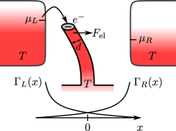
Figure 1: Two leads with chemical potentials $\mu_{L}$ and $\mu_{R}$ at temperature $T$ are placed at some distance. In between, a quantum dot (grey disk) is mounted on a nanopillar, which in turn is mounted on a larger solid at temperature $T$. The nanopillar has diameter $d$ (which is relevant for our final discussion) and can oscillate from left ($x<0$) to right($x>0$). The left/right bare tunneling rates $\Gamma_{L/R}(x)$ depend on the dot position as sketched at the bottom. If an electron jumps on the dot, an electrostatic force $F_{\text{el}}$ acts on the nanopillar towards the right. The sketch pictures experimental setups of Refs. Erbe et al. (2001); Scheible and Blick (2004); Kim et al. (2010a, b, 2012), but the theoretical description below holds for a wider range of self-oscillating nanosystems.

We model the dynamics of the dot and oscillator semi-classically by a coupled Fokker-Planck and master equation Wächtler et al. (2019a), which includes thermal fluctuations of the oscillator and allows us to study its entropy later on. In our regime of interest, quantum corrections to the oscillator are negligible . In Appendix A we derive our equation of motion below starting from the quantum description Novotný et al. (2003) and using phase space methods Faddeev and Yakubovskii (2009); Gardiner and Zoller (2004).

Let $P_{q}(x,v;t)$ be the probability density at time $t$ to find the oscillator at position $x$ (where $x=0$ defines the centre between the leads) with velocity $v$ and the dot with $q$ electrons. For simplicity we assume $q\in\{0,1\}$ (ultrastrong Coulomb blockade). This choice has little influence on the qualitative behaviour we are interested in, but we return to it at the end. Then, $P_{q}(x,v;t)$ obeys

$$\frac{\partial P_{q}(x,v;t)}{\partial t}=L_{q}P_{q}(x,v;t)+\sum_{q^{\prime}}R_{qq^{\prime}}(x)P_{q^{\prime}}(x,v;t),$$ (1)

where we defined the following objects. First,

$$L_{q}\equiv-v\frac{\partial}{\partial x}+\frac{\partial}{\partial v}\left[\frac{k}{m}x+\frac{\gamma}{m}v-\frac{e\alpha V}{m}q+\frac{\gamma}{\beta m^{2}}\frac{\partial}{\partial v}\right]$$ (2)

generates the oscillator movement as a function of the dot occupation $q$, where $k$ is the spring constant, $m$ the mass and the friction coefficient $\gamma=-F_{\text{damp}}/v$ results from a force $F_{\text{damp}}$ damping the oscillator in contact with an environment at inverse temperature $\beta=(k_{B}T)^{-1}$. The inverse distance $\alpha>0$ quantifies the strength of the electric field in between the leads and $V=(\mu_{L}-\mu_{R})/e$ denotes the voltage ($e>0$ is the elementary charge). The leads with chemical potential $\mu_{L}$ and $\mu_{R}$ are at the same temperature $T$. They influence the dynamics via the rate matrix $R(x)=R^{L}(x)+R^{R}(x)$, which can be split into contributions from the left and right lead and depends on the oscillator position $x$. Explicitly, the off-diagonal elements of $R^{L}(x)$ (the diagonal elements are fixed by probability conservation) describing the filling or depletion of the dot, respectively, read $R_{10}^{L}(x)=\Gamma_{L}(x)f_{L}[\epsilon(x)]$ and $R_{01}^{L}(x)=\Gamma_{L}(x)\{1-f_{L}[\epsilon(x)]\}$. Here, $\Gamma_{L}(x)=\Gamma_{0}e^{-x/\lambda}$ is an exponentially sensitive tunneling rate, $\Gamma_{0}$ a bare tunneling rate, $\lambda$ a characteristic tunneling distance and $f_{L}(\omega)=[e^{\beta(\omega-\mu_{L})}+1]^{-1}$ the Fermi function. Importantly, the charging energy $\epsilon(x)=\epsilon_{0}-e\alpha Vx$ of the filled dot is $x$-dependent ($\epsilon_{0}$ is some effective on-site energy). Finally, the rate matrix $R^{R}(x)$ of the right lead is obtained from $R^{L}(x)$ by replacing $f_{L}$ by $f_{R}$ and by setting $\Gamma_{R}(x)=\Gamma_{L}(-x)$ (symmetric tunneling rates).

We briefly discuss the thermodynamics of our autonomous model. The system (dot plus oscillator) is coupled to three baths: two electronic leads and the oscillator heat bath, labeled with a subscript ‘$O$’ below. The heat flow up to time $t$ from bath $\nu\in\{L,R,O\}$ is denoted $Q_{\nu}(t)$. The first law reads

$$\Delta U_{DO}(t)=\sum_{\nu}Q_{\nu}(t)+W_{\text{chem}}(t),$$ (3)

where $\Delta U_{DO}=U_{DO}(t)-U_{DO}(0)$ is the change in internal energy of the dot and oscillator (we set the initial time to $t=0$) and $W_{\text{chem}}(t)$ is the chemical work associated to the transport of electrons (defined positive if electrons flow along the bias). Since all baths have the same temperature, the second law becomes

$$\Delta S_{DO}(t)-\frac{1}{T}\sum_{\nu}Q_{\nu}(t)\geq 0$$ (4)

with $S_{DO}(t)$ denoting the Gibbs-Shannon entropy of $P_{q}(x,v;t)$.

We are only interested in average thermodynamic quantities. Therefore, the above analysis is quite standard and detailed definitions are postponed to Appendix B. In our numerical simulations, however, we compute all quantities as averages over stochastic trajectories as detailed in Ref. Wächtler et al. (2019a).

(ii) Reduced dynamics.—We now show how our autonomous model implements an idealized cycle in a certain parameter regime. Numerical simulations of Eq. (1) support our arguments.

First, we want the oscillator to act like a work reservoir, which is described by the ideal limit $m\rightarrow\infty$ while keeping $\omega=\sqrt{k/m}$ fixed Deffner and Jarzynski (2013). We argue below that this limit is actually ‘over-idealized,’ but for now it is instructive to consider it. Then, the generator (2) reduces to $L_{q}\rightarrow-v\partial_{x}+\partial_{v}\omega^{2}x$, which describes undisturbed motion of the oscillator according to the Hamiltonian $H_{O}(x,v)=mv^{2}/2+kx^{2}/2$. If the initial condition is $P_{q}(x,v;0)={\cal{P}}_{q}(0)\delta(x-x_{0})\delta(v)$, i.e., the oscillator starts at position $x_{0}$ with zero velocity, the state at time $t$ reads $P_{q}(x,v;t)={\cal{P}}_{q}(t)\delta(x-x_{t})\delta(v-v_{t})$ with $x_{t}=x_{0}\cos(\omega t)$ and $v_{t}=\dot{x}_{t}$. Thus, there is no backaction from the dot on the oscillator. However, the oscillator still influences the dot, which now obeys a time-dependent master equation:

$$\frac{\partial{\cal{P}}_{q}(t)}{\partial t}=\sum_{q^{\prime}}R_{qq^{\prime}}(x_{t}){\cal{P}}_{q^{\prime}}(t).$$ (5)

The solution of Eq. (5), and quantities derived from it, is distinguished from the solution of the full dynamics (1) by using calligraphic symbols such as ${\cal{P}}_{q}$.

In reality, the above limit is too strong as it implies a constant oscillator energy: $dH_{O}(x_{t},v_{t})/dt=0$. This is unphysical because Eq. (5) predicts a finite energy flow into the oscillator (see below). Of course, in reality any oscillator mass is finite, albeit it can be very large. An adequate description is achieved by replacing $x_{t}$ with $\tilde{x}_{t}=a_{t}\cos(\omega t)$, where $a_{t}$ is the amplitude of the oscillator starting from $a_{0}=x_{0}$. For large but finite mass $m$, $a_{t}$ varies slowly in time, i.e., $a_{t}=x_{0}(1+\delta_{t})$ with $|\dot{\delta}_{t}|\ll\omega$. Furthermore, for times $t$ such that $|\delta_{t}|\ll 1$, Eq. (5) remains a good approximation while at the same time there is a finite change in oscillator energy because the evaluation of $H_{O}(x_{t},v_{t})-H_{O}(x_{0},v_{0})$ involves terms like $\delta_{t}mx_{0}$, which can be large.

The previous point is very important. The limit $m\rightarrow\infty$ is inconsistent, whereas the regime of finite but large $m$ makes our analysis consistent and non-trivial. From an analytical and numerical perspective, this is challenging as we can not rely on a steady state analysis of Eq. (1). To capture thermodynamic changes of the oscillator, we have to take into account its transient dynamics.

Finally, we justify the analysis in terms of a thermodynamic cycle divided into strokes (cf. Figs. 1 and 2 and Appendix C). First, the (approximately) periodic motion of the oscillator gives us the duration $\tau_{\text{cycle}}=2\pi/\omega$ of one cycle. Next, if $x_{0}$ and $\lambda$ are chosen appropriately, the exponential sensitivity of the tunneling rates $\Gamma_{L/R}(x_{t})$ justifies to neglect the influence of both leads when the dot is in the centre and to neglect the influence of the left (right) lead when the dot is on the right (left). The first case, determined by $\Gamma_{L/R}(x_{t})\approx 0$, realizes an isentropic stroke, where the dot does not change its state while its energy changes due to its movement in the potential bias. The second case, determined by $\Gamma_{L}(x_{t})\gg 0$ or $\Gamma_{R}(x_{t})\gg 0$, realizes a dissipative stroke, where, both, the state and energy of the dot changes. If parameters are fine-tuned such that the dot remains at temperature $T$, this stroke is isothermal. In general, however, the dot is out of equilibrium in our setup.

Thus, we find that the cycle description is justified if

$$e^{|x_{0}|/\lambda}\gg 1,~{}~{}~{}\tau_{\text{isen}}\Gamma_{0}\exp\left[\frac{|x_{0}|}{\lambda}\sin\left(\frac{\omega\tau_{\text{isen}}}{2}\right)\right]\ll 1.$$ (6)

The first condition in Eq. (6) is necessary to neglect the effect of the opposite, remote lead during the dissipative strokes. The second condition involves the duration $\tau_{\text{isen}}$ of the isentropic strokes, which depends on other parameters of the model. It is derived in detail in Appendix C.

We are particularly interested in the properties of our device as a function of the oscillator mass $m$ (keeping $\omega$ fixed) and the friction coefficient $\gamma$. The other parameters are based on reasonable estimates from Refs. Kim et al. (2007, 2010a, 2010b, 2012); Prada and Platero (2012), precisely listed in Appendix D. For them we find a duration $\tau_{\text{isen}}=\tau_{\text{cycle}}/12$ of the isentropic stroke in unison with condition (6) with a total cycle time $\tau_{\text{cycle}}\approx 25$ ns.

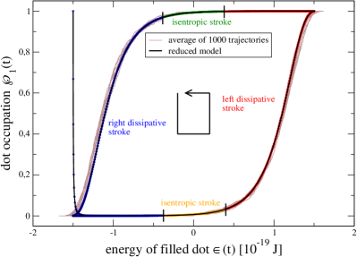
Figure 2: Parametric plot of the dot occupation and energy $\epsilon(t)=\epsilon_{0}-\alpha eVx_{t}$, which is in one-to-one correspondence with the oscillator position $x_{t}$ ($\epsilon_{0}=0$ here). We compare the solution of Eq. (5) with unperturbed oscillator trajectory $x_{t}=x_{0}\cos(\omega t)$ (black and dotted) with the average of 1000 stochastic trajectories of the full dynamics (1) (thin brown) with identical initial condition for $t\in[0,250{\rm ns}]$. The system quickly reaches a limit cycle, where the enclosed area measures the extracted work per cycle.

(iii) Reduced thermodynamics.—We start with the analysis of Eq. (5), distinguished by calligraphic symbols. For now, we ignore the fact that Eq. (5) follows from an underlying autonomous model—instead, we assume that the time-dependent rate matrix is generated by an ideal work reservoir as conventionally done in thermodynamic cycle analyses Vinjanampathy and Anders (2016); Kosloff and Rezek (2017); Ghosh et al. (2018); Feldmann and Palao (2018); Levy and Gelbwaser-Klimovsky (2018); Deffner and Campbell (2019). Then, mechanical work becomes

$${\cal{W}}_{\rm mech}(t)=\int_{0}^{t}dt^{\prime}{\cal{P}}_{1}(t^{\prime})\frac{\partial\epsilon(x_{t^{\prime}})}{\partial t^{\prime}}.$$ (7)

For a single cycle the work equals the area enclosed by the limit cycle trajectory (counted positive in clockwise direction in Fig. 2), similar to a $p$–$V$ diagram in traditional cycles.

As before, there are heat flows ${\cal{Q}}_{\nu}(t)$ from lead $\nu$ and chemical work ${\cal{W}}_{\text{chem}}(t)$ such that the first law reads

$$\Delta{\cal{U}}_{D}(t)={\cal{Q}}_{L}(t)+{\cal{Q}}_{R}(t)+{\cal{W}}_{\rm chem}(t)+{\cal{W}}_{\rm mech}(t).$$ (8)

Here, ${\cal{U}}_{D}(t)=\epsilon(x_{t}){\cal{P}}_{1}(t)$ is the internal energy of the dot. Furthermore, denoting by ${\cal{S}}_{D}(t)$ the Gibbs-Shannon entropy of ${\cal{P}}_{q}(t)$, the second law reads

$$\Delta{\cal{S}}_{D}(t)-\frac{1}{T}[{\cal{Q}}_{L}(t)+{\cal{Q}}_{R}(t)]\geq 0.$$ (9)

This analysis follows again from standard considerations and explicit expressions are thus only displayed in Appendix E. Note that Eqs. (8) and (9), while mathematically true, need not coincide with the thermodynamics of the autonomous model. In general, the dot dynamics predicted by both methods differ, i.e., ${\cal{P}}_{q}(t)\neq P_{q}(t)\equiv\int dxdvP_{q}(x,v;t)$.

We now return to the first and second law of the autonomous model, Eqs. (3) and (4), rewritten as (dropping the $t$-dependence for simplicity)

$$\Delta U_{D}=Q_{L}+Q_{R}+W_{\text{chem}}+Q_{O}-\Delta U_{O},$$ (10)

$$\Delta S_{D}-\frac{Q_{L}}{T}-\frac{Q_{R}}{T}+\Delta S_{O|D}-\frac{Q_{O}}{T}\geq 0.$$ (11)

Here, the oscillator energy $U_{O}$ equals the expectation value of its Hamiltonian $H_{O}(x,v)$ and $S_{O|D}=S_{DO}-S_{D}$ is the conditional entropy. The necessary conditions for the thermodynamic laws (8) and (9) of the reduced model to coincide with Eqs. (10) and (11) follow as

$$\frac{Q_{O}}{T}=0~{}~{}~{}\text{and}~{}~{}~{}\Delta S_{O|D}=0.$$ (12)

Of course, on top of that, we also need ${\cal{P}}_{q}(t)=P_{q}(t)$.

Even if all parameters are kept finite in the original model, the above conditions can be satisfied to good approximation. First, for large mass $m$, keeping $k/m$ fixed, the dynamics is well-described by Eq. (5), i.e., ${\cal{P}}_{q}(t)\approx P_{q}(t)$. We checked this numerically for multiple parameters, see Fig. 2 for a particular example. Furthermore, the solution of Eq. (1) remains approximately of the form $P_{q}(x,v;t)\approx{\cal{P}}_{q}(t)\delta(x-x_{t})\delta(v-v_{t})$, i.e., the oscillator state has low entropy for long times, which implies $\Delta S_{O|D}\approx 0$ (dash-dotted grey line in Fig. 3).

The previous argument is not yet sufficient to conclude that $Q_{O}/T\approx 0$. Instead, the heat flow $Q_{O}$ is controlled by the friction coefficient $\gamma$. Thus, on top of the large $m$ regime, we also require small $\gamma$. Then, Eqs. (10) and (11) coincide with Eqs. (8) and (9). In this limit, the oscillator resembles a perfect work reservoir or battery.

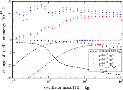
Figure 3: Average energy change of the oscillator $\Delta U_{O}$ (with error bars marking the statistical error) over the time interval $[0,250{\rm ns}]$ versus mass for different friction coefficients (in logarithmic scale). Dashed curves of matching color correspond to the heat flow $Q_{O}$ from the oscillator bath. As $\gamma\to 0$ and $m\to\infty$, $\Delta U_{O}$ matches $-{\cal{W}}_{\text{mech}}$ (dash-dotted blue line) and $Q_{O}$ and $\Delta S_{O|D}$ become negligible.

These arguments are exemplified in Fig. 3. First, for increasing $m$, we see that we obtain $\Delta U_{O}-Q_{O}\approx-{\cal{W}}_{\text{mech}}$. Second, we observe for decreasing $\gamma$ that $Q_{O}\rightarrow 0$. Hence, $\Delta U_{O}=-{\cal{W}}_{\text{mech}}$ and the mechanical work computed from the reduced dynamics (5) is stored as extractable energy in the oscillator since $T|\Delta S_{O}|\ll|\Delta U_{O}|$.

The question remains whether also the cycle analysis matches this picture. However, if condition (6) is satisfied, then the dynamics of the master equation (5) matches the cycle dynamics. This is constructed by time-evolving the state ${\cal{P}}_{q}(t)$ only with respect to the rate matrix $R^{L}(x_{t})$ [$R^{R}(x_{t})$] during the left [right] dissipative stroke and by using the identity map for the isentropic strokes. In this regime, the thermodynamic quantities in Eqs. (8) and (9) coincide by construction with the cycle analysis, demonstrated in detail in Appendix F.

Experimental feasibility.—Can thermodynamic cycles realistically be used to analyse nanoscale engines? Based on our parameter choice (see Appendix D), we find the following. First, the experimentally used mass $m$ is already sufficiently large, albeit an increase in it would still be beneficial. Second, to mimic an ideal work reservoir, the friction $\gamma$ needs to be about one order of magnitude smaller than typical experimental values. This could be in reach with current technologies. Third, as stated in the SM, our numerics is based on a large voltage $V$. This likely invalidates the ultrastrong Coulomb blockade assumption and raises the final question: is a cycle with a single-electron working fluid realistic?

To answer it, we estimate the number $N$ of electrons contributing to the transport in the ‘bias window’ $\Delta E\equiv eV$. The electrostatic energy of the dot is $E_{D}=(eN)^{2}/(2C)$, where $C\approx 4\pi\epsilon_{0}d$ is the self capacitance of the dot mounted on the nanopillar with diameter $d$ . Equating $\Delta E=E_{D}$, we obtain $N^{2}\approx 3.5\cdot 10^{10}\cdot d/$m for our parameter choice. For $N=1$ (the case considered here), this requires a nanopillar with a diameter of 30 pm. This is smaller than the radius of a hydrogen atom and impossible to fabricate. Hence, we assume a diameter of 5 nm for stability reasons, which is optimistic compared to experimental values of $d=60$ nm Kim et al. (2010a). Then, we obtain the estimate $N\approx 13$. We conclude that an autonomous implementation of a thermodynamic cycle with a single-electron working medium seems experimentally impossible, but $N\gtrsim 10$ electrons could suffice.

Our conclusions seem to remain for other experimental platforms , but a recent experiment Wen et al. (2020) reports sustained oscillations of a suspended carbon nanotube for $N=1$ electron. However, in view of our Fig. 1, the nanotube oscillates vertically (i.e., up–down instead of left–right), which makes the identification of strokes unclear. Nevertheless, it remains an intriguing question whether the nanotube acts like an ideal work reservoir.

We remark that we have not shown how to implement a Carnot or Otto cycle. Our cycle is driven by a voltage instead of temperature bias, converting chemical work into mechanical work. Autonomously realizing Carnot and Otto cycles faces additional challenges and remains open.

Conclusions.—We demonstrated the potential of self-oscillating engines to address problems of foundational and practical relevance. These models could pave the way for fruitful future research avenues, as evidenced also by other recent studies Tonekaboni et al. (2018); Wächtler et al. (2019a, b); Filliger and Reimann (2007); Wang et al. (2008); Alicki et al. (2015); Serra-Garcia et al. (2016); Alicki (2016); Chiang et al. (2017); Roulet et al. (2017); Alicki et al. (2017); Seah et al. (2018); Alicki et al. (2020).

Acknowledgements.—PS is financially supported by the DFG (project STR 1505/2-1), the Spanish Agencia Estatal de Investigación, project PID2019-107609GB-I00, the Spanish MINECO FIS2016-80681-P (AEI/FEDER, UE), and Generalitat de Catalunya CIRIT 2017-SGR-1127. CWW and GS acknowledge support by the DFG through Project No. BR1528/8-2. CWW acknowledges support from the Max-Planck Gesellschaft via the MPI-PKS Next Step fellowship.

Appendix A Derivation of the coupled Fokker-Planck and master equation

Our starting point is the full quantum master equation for the combined dot-oscillator system as derived in Ref. Novotný et al. (2003):

$$\frac{\partial}{\partial t}\hat{\rho}(t)= ~{}({\cal{L}}_{\text{coh}}+{\cal{L}}_{\text{drive}}+{\cal{L}}_{\text{damp}})\hat{\rho}(t),$$ (13)

$${\cal{L}}_{\text{coh}}\hat{\rho}= ~{}\frac{1}{\rm i\hbar}[H_{\text{osc}}+\epsilon_{0}\hat{c}_{0}^{\dagger}\hat{c}_{0}-eE\hat{x}\hat{c}_{0}^{\dagger}\hat{c}_{0},\hat{\rho}],$$ (14)

$${\cal{L}}_{\text{drive}}\hat{\rho}= -\frac{\Gamma_{L}}{2}\left(\hat{c}_{0}\hat{c}_{0}^{\dagger}e^{-2\hat{x}/\lambda^{\prime}}\hat{\rho}-2\hat{c}_{0}^{\dagger}e^{-\hat{x}/\lambda^{\prime}}\hat{\rho}e^{-\hat{x}/\lambda^{\prime}}\hat{c}_{0}+\hat{\rho}e^{-2\hat{x}/\lambda^{\prime}}\hat{c}_{0}\hat{c}_{0}^{\dagger}\right)$$ (15)

$$-\frac{\Gamma_{R}}{2}\left(\hat{c}_{0}^{\dagger}\hat{c}_{0}e^{2\hat{x}/\lambda^{\prime}}\hat{\rho}-2\hat{c}_{0}e^{\hat{x}/\lambda^{\prime}}\hat{\rho}e^{\hat{x}/\lambda^{\prime}}\hat{c}^{\dagger}_{0}+\hat{\rho}e^{2\hat{x}/\lambda^{\prime}}\hat{c}_{0}^{\dagger}\hat{c}_{0}\right),$$

$${\cal{L}}_{\text{damp}}\hat{\rho}= -\frac{\rm i\gamma^{\prime}}{2\hbar}[\hat{x},\{\hat{p},\hat{\rho}\}]-\frac{\gamma^{\prime}m\omega}{\hbar}\left(\bar{N}+\frac{1}{2}\right)[\hat{x},[\hat{x},\hat{\rho}]].$$ (16)

Here, we mostly followed the notation of Ref. Novotný et al. (2003), but explicitly denoted operators with a hat for convenience. The notation of the main text is obtained after identifying $H_{\text{osc}}=H_{O}$, $\lambda^{\prime}=2\lambda$, $E=\alpha V$ and $\gamma^{\prime}=\gamma/m$ (note that the friction coefficient $\gamma$ in the main text does not have the dimension of a rate in contrast to $\gamma^{\prime}$). Furthermore, $\hat{c}_{0}^{\dagger}$ ($\hat{c}_{0}$) creates (annihilates) an electron on the dot and $\bar{N}=(e^{\beta\hbar\omega}-1)^{-1}$ is the Bose-Einstein distribution. Finally, we point out that the master equation in Ref. Novotný et al. (2003) was derived in the ‘high-bias’ limit, which allowed them to replace the Fermi functions by $f_{L}(\omega)\approx 1$ and $f_{R}(\omega)\approx 0$ for all dot energies $\omega$. For simplicity in the presentation and in unison with Ref. Novotný et al. (2003) we keep the Fermi function out of the discussion here.

For the reasons spelled out in Footnote [62] of the main text, we are interested in the classical limit of the quantum master equation above. This is most conveniently derived by considering the time-evolution of the Wigner function $W(x,p)$ of the oscillator (where $p$ is its momentum) and by taking the formal limit $\hbar\rightarrow 0$ Faddeev and Yakubovskii (2009). Moreover, we are only interested in the occupation probabilities of the dot as coherences between the empty and filled state of the dot are prohibited since they correspond to superpositions of different charged states. Thus, we define

$$W_{q}(x,p)=\frac{1}{\hbar\pi}\int_{-\infty}^{\infty}dy\langle x-y,q|\hat{\rho}|x+y,q\rangle e^{2\rm ipy/\hbar},$$ (17)

where $q\in\{0,1\}$ denotes the number of electrons on the dot. The time-evolution of $W_{q}(x,p)$ can then be derived from Eq. (13) by using operator correspondence rules, which can be readily checked for consistency in textbooks Gardiner and Zoller (2004). Examples are

$$\hat{x}\hat{\rho}\mapsto\left(x+\frac{\rm i\hbar}{2}\frac{\partial}{\partial p}\right)W_{q}(x,p),~{}~{}~{}\hat{p}\hat{\rho}\mapsto\left(p-\frac{\rm i\hbar}{2}\frac{\partial}{\partial x}\right)W_{q}(x,p),~{}~{}~{}\dots,$$ (18)

from which we can already confirm the position-momentum commutation relation. Multiplication from the right with these operators follows from Hermitian conjugation, as does a combination of them (provided one minds the correct ordering).

We find for the first term in Eq. (13) that

$${\cal{L}}_{\text{coh}}\hat{\rho}\mapsto\left[-\frac{\partial}{\partial x}\frac{p}{m}+\frac{\partial}{\partial p}(kx-eEq)\right]W_{q}(x,p),$$ (19)

without any need to take the limit $\hbar\rightarrow 0$. After setting $v=p/m$, Eq. (19) reproduces the first, second and fourth term of the generator $L_{q}$ defined in Eq. (2) of the main text.

Next, we consider the second term ${\cal{L}}_{\text{drive}}\hat{\rho}(t)$ in Eq. (13). The exponential factors $e^{\hat{x}/\lambda^{\prime}}$ in it make the mapping complicated in principle, but remember that we are only interested in the limit $\hbar\rightarrow 0$. Since $\hbar$ appears nowhere explicitly in ${\cal{L}}_{\text{drive}}$, we can directly use $\lim_{\hbar\rightarrow 0}\hat{x}\hat{\rho}\mapsto xW_{q}(x,p)$, which follows from Eq. (18). Thus, we can set, e.g., $\lim_{\hbar\rightarrow 0}e^{\hat{x}/\lambda^{\prime}}\hat{\rho}\mapsto e^{x/\lambda^{\prime}}W_{q}(x,p)$ and we obtain

$$\begin{split}\lim_{\hbar\rightarrow 0}{\cal{L}}_{\text{drive}}\hat{\rho}\mapsto&-\frac{\Gamma_{L}}{2}e^{-2x/\lambda^{\prime}}\left(\hat{c}_{0}\hat{c}_{0}^{\dagger}W(x,p)-2\hat{c}_{0}^{\dagger}W(x,p)\hat{c}_{0}+W(x,p)\hat{c}_{0}\hat{c}_{0}^{\dagger}\right)\\ &-\frac{\Gamma_{R}}{2}e^{2x/\lambda^{\prime}}\left(\hat{c}_{0}^{\dagger}\hat{c}_{0}W(x,p)-2\hat{c}_{0}W(x,p)\hat{c}^{\dagger}_{0}+W(x,p)\hat{c}_{0}^{\dagger}\hat{c}_{0}\right).\\ \end{split}$$ (20)

Here, we have not yet taken matrix element $|q\rangle$ in the dot basis. Doing so reveals that

$$\lim_{\hbar\rightarrow 0}{\cal{L}}_{\text{drive}}\hat{\rho}\mapsto\sum_{q^{\prime}}R_{qq^{\prime}}(x)W_{q^{\prime}}(x,p),$$ (21)

where $R_{qq^{\prime}}(x)$ is the rate matrix defined in the main text in the high bias limit (as discussed above).

Finally, the last term ${\cal{L}}_{\text{damp}}\hat{\rho}(t)$ in Eq. (13) simply describes the dynamics of a damped harmonic oscillator. It reduces to the third and fifth term of the generator $L_{q}$ defined in Eq. (2) of the main text for $\hbar\rightarrow 0$, after paying attention to the fact that $\gamma^{\prime}=\gamma/m$. Thus, after setting $P_{q}(x,v;t)\equiv W_{q}(x,mv)$, we obtain Eq. (1) of the main text as the classical limit of the quantum master equation derived in Ref. Novotný et al. (2003). Note that in the classical limit $P_{q}(x,v;t)=W_{q}(x,mv)$ has no negativities and becomes a well defined probability density.

Appendix B Precise thermodynamic definitions for the autonomous model

We define the internal energy and entropy of the combined dot-oscillator system as

$$U_{DO}(t)\equiv\sum_{q}\int dxdv\left[\frac{mv^{2}}{2}+\frac{kx^{2}}{2}+\epsilon(x)q\right]P_{q}(x,v;t),~{}~{}~{}S_{DO}(t)\equiv-k_{B}\sum_{q}\int dxdvP_{q}(x,v;t)\ln\left[\frac{\hbar}{m}P_{q}(x,v;t)\right].$$ (22)

We remark that the factor $\hbar/m$, which ensures that the argument of the logarithm is dimensionless, cancels out whenever we take differences of $S_{DO}(t)$. This is always the case in the following. Furthermore, the instantaneous heat flow from lead $\nu\in\{L,R\}$ is composed out of an energy and a particle current: $\dot{Q}_{\nu}(t)=J_{\nu}(t)-\mu_{\nu}I_{\nu}(t)$. They are defined as

$$J_{\nu}(t)\equiv\sum_{q,q^{\prime}}\int dxdv(\epsilon_{0}-\alpha eVx)qR^{\nu}_{q,q^{\prime}}(x)p_{q^{\prime}}(x,v;t),~{}~{}~{}I_{\nu}(t)\equiv\sum_{q,q^{\prime}}\int dxdvqR_{q,q^{\prime}}^{\nu}(x)p_{q^{\prime}}(x,v;t).$$ (23)

The instantaneous heat flow from the oscillator bath $\dot{Q}_{O}(t)$ only has an energy component:

$$\dot{Q}_{O}(t)=\sum_{q}\int dxdv\left(\frac{mv^{2}}{2}+\frac{kx^{2}}{2}-\alpha eVxq\right)L_{q}P_{q}(x,v;t).$$ (24)

The heat flows appearing in the first law (3) in the main text follow by integration: $Q_{\nu}(t)=\int_{0}^{t}dt^{\prime}\dot{Q}_{\nu}(t^{\prime})$, $\nu\in\{L,R,O\}$. Finally, the chemical work is defined as

$$W_{\text{chem}}(t)\equiv\int_{0}^{t}dt^{\prime}\left[\mu_{L}I_{L}(t^{\prime})+\mu_{R}I_{R}(t^{\prime})\right].$$ (25)

Appendix C Partitioning the cycle into strokes

The emergence of different strokes in our analysis arises from the sensitivity of the bare tunneling rates $\Gamma_{L/R}(x_{t})$ with respect to the changing position $x_{t}$ of the oscillator as sketched in Fig. 4. If $\Gamma_{L}(x_{t})\gg\Gamma_{R}(x_{t})\approx 0$ [$\Gamma_{R}(x_{t})\gg\Gamma_{L}(x_{t})\approx 0$], the oscillator is on the left [right] and we can neglect the influence of the opposite lead, which defines the respective dissipative strokes. If $\Gamma_{L}(x_{t})\approx\Gamma_{R}(x_{t})\approx 0$, the oscillator is in the middle, which defines the isentropic strokes. Whether these strokes can be identified and how long they last depends on the precise choice of numerical parameters. Below, we estimate the time $\tau_{\text{isen}}$ that the oscillator spends in the centre with negligible influence from both leads, i.e., we ask when is $\Gamma_{L}(x_{t})\approx\Gamma_{R}(x_{t})\approx 0$. This gives us the second condition in Eq. (6) in the main text.

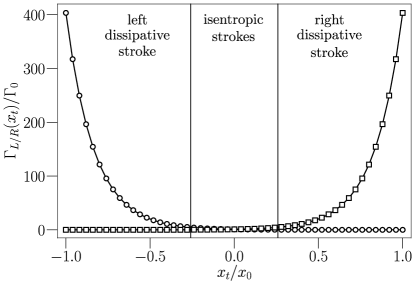
Figure 4: Plot of the bare tunneling rates $\Gamma_{L}(x_{t})$ (circles) and $\Gamma_{R}(x_{t})$ (squares) as a function of the oscillator trajectory $x_{t}=x_{0}\cos(\omega t)$ obtained in the limit of an ideal work reservoir for the numerical parameters specified in Sec. D. The regimes where we identify the different strokes are separated by vertical lines. We remark that the precise numerical definition of the strokes requires to introduce a threshold value and is therefore only fixed with respect to that value. To be on the safe side, we choose our threshold value such that the integral (26) is much smaller than one. Then, at the boundary of the isentropic stroke, the dot is still hardly coupled to any of the leads, and small changes of the cycle durations will have no net effect.

The time evolution of the dot is given by the time-ordered exponential of the rate matrix appearing in Eq. (5) in the main text and we seek to find the time-intervals in which this is approximately equal to the identity, i.e., the state of the dot remains unchanged. The length of this ‘isentropic’ time interval is denoted $\tau_{\text{isen}}$ in the following. Clearly, by symmetry these time-interval are centered around the times $\pi(n+\frac{1}{2})/\omega$ ($n\in\mathbb{N}$) when the oscillator is in the centre around $x_{t}\approx 0$ [note that the initial condition for the oscillator is $(x_{0},v_{0})=(|x_{0}|,0)$, see Sec. D]. To determine the length $\tau$ of, say, the first time-interval, we demand that

$$I\equiv\int\limits_{\frac{\pi}{2\omega}-\frac{\tau_{\text{isen}}}{2}}^{\frac{\pi}{2\omega}+\frac{\tau_{\text{isen}}}{2}}dt\left[\Gamma_{L}(x_{t})+\Gamma_{R}(x_{t})\right]\ll 1.$$ (26)

Here, $\Gamma_{L}(x_{t})=\Gamma_{0}e^{-x_{t}/\lambda}=\Gamma_{R}(-x_{t})$ are the bare tunneling rates for the left and right lead ignoring the influence of the Fermi functions. Since the Fermi functions are always smaller than one, neglecting them only underestimates the length $\tau_{\text{isen}}$.

Nevertheless, an exact analytical evaluation of the integral (26) is still not possible. Therefore, we make further approximations. First, we assume the necessary requirement $\exp(|x_{0}|/\lambda)\gg 1$, i.e., the first condition of Eq. (6) in the main text, to be satisfied. Together with our choice for the initial state of the oscillator, we simplify

$$I\approx\int\limits_{\frac{\pi}{2\omega}-\frac{\tau_{\text{isen}}}{2}}^{\frac{\pi}{2\omega}}\Gamma_{L}(x_{t})dt+\int\limits_{\frac{\pi}{2\omega}}^{\frac{\pi}{2\omega}+\frac{\tau_{\text{isen}}}{2}}\Gamma_{R}(x_{t})dt\ll 1.$$ (27)

This step undestimates the value of $I$, but this is well compensated by the next crude approximation, where we replace $\Gamma_{L}(x_{t})$ and $\Gamma_{R}(x_{t})$ by their maximum values taken at the boundaries for $t=\frac{\pi}{2\omega}-\frac{\tau_{\text{isen}}}{2}$ and $t=\frac{\pi}{2\omega}+\frac{\tau_{\text{isen}}}{2}$, respectively. Then,

$$I\approx\frac{\tau_{\text{isen}}}{2}\Gamma_{L}\left(x_{\pi/2\omega-\tau_{\text{isen}}/2}\right)+\frac{\tau_{\text{isen}}}{2}\Gamma_{R}\left(x_{\pi/2\omega+\tau_{\text{isen}}/2}\right)=\tau_{\text{isen}}\Gamma_{0}\exp\left[\frac{|x_{0}|}{\lambda}\sin\left(\frac{\omega\tau_{\text{isen}}}{2}\right)\right],$$ (28)

where we used the identity $\cos(\pi/2\pm x)=\mp\sin(x)$. Now, the requirement that $I\ll 1$ gives the second condition in Eq. (6) in the main text.

For the numerical parameters listed in Sec. D below, we find a partition into strokes as summarized in Table 1.

	stroke	time interval $[\tau_{\text{cycle}}]$
(a)	right dissipative stroke	$\left[0,\frac{5}{24}\right)\cup\left[\frac{19}{24},1\right)$
(b)	isentropic stroke	$\left[\frac{5}{24},\frac{7}{24}\right)$
(c)	left dissipative stroke	$\left[\frac{7}{24},\frac{17}{24}\right)$
(d)	isentropic stroke	$\left[\frac{17}{24},\frac{19}{24}\right)$

Table 1: Division of the cycle into four strokes such that Eq. (6) in the main text is satisfied.

Appendix D Parameter choice for numerical simulations

The electron shuttle can be realized using different experimental setups. We here focus on the case where the oscillatory degree of freedom is a nanopillar as sketched in Fig. 1 in the main text and realized in Refs. Kim et al. (2007, 2010a, 2010b, 2012). The material parameters typical for such experiments and used in this work are summarized below and in Table 2.

The bias voltage for electron shuttles can be tuned over a large regime. Here, we use a value of $V=25$V, which is a bit larger than experimentally reported values, but guarantees a clearly visible regime of self-oscillations and a simpler numerical treatment. We remark that the threshold value for the onset of self-oscillations is in our model around $V^{*}\approx 10$ V for the parameters chosen here. In reality, for $V=25$V we no longer expect the ultrastrong Coulomb blockade assumption to work well, which means that multiple electrons can hop on the dot. Importantly, this effect does not change the general conclusions reported in this paper and it can be easily accounted for (see the final conclusions in the main text). Furthermore, in all our calculations we choose a temperature of $T=1$K and set the chemical potentials as $\mu_{L}=\epsilon_{0}+eV/2$ and $\mu_{R}=\epsilon_{0}-eV/2$, which eliminates the dependence on the on-site energy $\epsilon_{0}$ in all equations.

Since we consider transient dynamics, the choice of initial conditions and running time is important. Here, we choose the initial conditions $x_{0}=6.0$ nm, $v_{0}=0.0~{}\text{nm}/\text{ns}$ and $P_{q}(0)=\delta_{q,1}$ (filled dot). The simulation runs for $t_{f}=250$ ns, which corresponds to roughly 150 cycles, and we average over 1000 trajectories.

Parameter	Value	Units	Source
$\omega$	$0.25$	GHz	Kim et al. (2010b)
$m$	$20\times 10^{-19}$	kg	Kim et al. (2010b, 2012)
$\lambda$	$1$	nm	Kim et al. (2012)
$\alpha$	$0.01$	$\text{nm}^{-1}$	Estimated from Kim et al. (2007, 2010a)
$\gamma$	$0.05\times 10^{-10}$	$\text{kg}/\text{s}$	Kim et al. (2012)
$\Gamma_{0}$	$0.01$	GHz	Kim et al. (2012)
$V$	$25.0$	V
$T$	$1$	K

Table 2: Parameters used in this work.

Appendix E Precise thermodynamic definitions for the reduced model

The internal energy and entropy of the dot are defined as follows:

$${\cal{U}}_{D}(t)\equiv\sum_{q}[\epsilon_{0}-\alpha eVx(t)]q{\cal{P}}_{q}(t),~{}~{}~{}{\cal{S}}_{D}(t)\equiv-k_{B}\sum_{q}{\cal{P}}_{q}(t)\ln{\cal{P}}_{q}(t).$$ (29)

The heat flow and chemical work rate are composed out of the energy and matter fluxes as usual: $\dot{{\cal{Q}}}_{\nu}(t)={\cal{J}}_{\nu}(t)-\mu_{\nu}{\cal{I}}_{\nu}(t)$ and $\dot{{\cal{W}}}_{\text{chem}}(t)=\sum_{\nu}\mu_{\nu}{\cal{I}}_{\nu}(t)$. They are defined as

$${\cal{I}}_{\nu}(t)\equiv\sum_{q,q^{\prime}}qR_{q,q^{\prime}}^{\nu}(x_{t}){\cal{P}}_{q^{\prime}}(t),~{}~{}~{}{\cal{J}}_{\nu}(t)\equiv[\epsilon_{0}-\alpha eVx(t)]{\cal{I}}_{\nu}(t).$$ (30)

Appendix F Cycle analysis of the reduced model in terms of thermodynamic strokes

In this section we denote by $\tau_{a,b,c,d}$ the time-intervals defined in Table 1 for brevity. Furthermore, for definiteness we focus on the analysis of the first cycle $[0,\tau_{\text{cycle}}]$. Extending our result below to further cycles is merely a matter of notation.

Based on this, the state of the dot within the cycle analysis at time $t\in[0,\tau_{\text{cycle}}]$, denoted $[{\cal{P}}_{q}(t)]_{\text{cycle}}$, can be written in the compact form

$$[{\cal{P}}_{q}(t)]_{\text{cycle}}={\cal{T}}_{+}\exp\left\{\int_{\tau_{a}\cap[0,t]}dtR^{L}(x_{t})+\int_{\tau_{c}\cap[0,t]}dtR^{R}(x_{t})\right\}{\cal{P}}_{q}(0),$$ (31)

where ${\cal{T}}_{+}$ denotes the time-ordering operator. If condition (6) in the main text is satisfied, then we have

$$[{\cal{P}}_{q}(t)]_{\text{cycle}}\approx{\cal{P}}_{q}(t)={\cal{T}}_{+}\exp\left\{\int_{0}^{t}dt[R^{L}(x_{t})+R^{R}(x_{t})]\right\}{\cal{P}}_{q}(0).$$ (32)

The claim is now that this is sufficent to demonstrate that the thermodynamic analysis of the cycle coincides with the analysis of Sec. E.

To this end, we first note that the definition of the state functions internal energy and system entropy are the same as in Sec. E, see Eq. (29), with ${\cal{P}}_{q}(t)$ replaced by $[{\cal{P}}_{q}(t)]_{\text{cycle}}$. Thus, clearly, if ${\cal{P}}_{q}(t)\approx[{\cal{P}}_{q}(t)]_{\text{cycle}}$, then

$${\cal{U}}_{D}\approx[{\cal{U}}_{D}]_{\text{cycle}}~{}~{}~{}\text{and}~{}~{}~{}{\cal{S}}_{D}\approx[{\cal{S}}_{D}]_{\text{cycle}},$$ (33)

where we used $[{\cal{X}}]_{\text{cycle}}$ to denote a thermodynamic quantity ${\cal{X}}$ in our cycle analysis. Furthermore, the definition of mechanical work during stroke $s$ ($s\in\{a,b,c,d\}$) is

$$[{\cal{W}}_{\rm mech}^{(s)}]_{\text{cycle}}=\int_{\tau_{s}}dt[{\cal{P}}_{1}(t)]_{\text{cycle}}\frac{\partial\epsilon(x_{t})}{\partial t}.$$ (34)

Again, if ${\cal{P}}_{q}(t)\approx[{\cal{P}}_{q}(t)]_{\text{cycle}}$, we clearly have

$$\sum_{s}[{\cal{W}}_{\rm mech}^{(s)}]_{\text{cycle}}\approx{\cal{W}}_{\text{mech}}=\int_{0}^{\tau_{\text{cycle}}}dt{\cal{P}}_{1}(t)\frac{\partial\epsilon(x_{t})}{\partial t}.$$ (35)

We now continue with a step-by-step analysis of the thermodynamic cyle

1. Left dissipative stroke: The dot is only coupled to the left lead and the first and second law read

   $$\Delta{\cal{U}}_{S}=[{\cal{Q}}_{L}]_{\text{cycle}}+[{\cal{W}}_{\text{chem}}]_{\text{cycle}}+{\cal{W}}_{\text{mech}},~{}~{}~{}\Delta S_{D}-[{\cal{Q}}_{L}]_{\text{cycle}}/T\geq 0.$$ (36)

   The not yet defined quantities appearing here are

   $$[{\cal{Q}}_{L}]_{\text{cycle}}=\int_{\tau_{a}}dt[{\cal{J}}_{L}(t)-\mu_{L}{\cal{I}}_{L}(t)],~{}~{}~{}[{\cal{W}}_{\text{chem}}]_{\text{cycle}}=\int_{\tau_{a}}dt\mu_{L}I_{L}(t)$$ (37)

   with the energy and matter current defined in Eq. (30).

2. Isentropic stroke: One has

   $$\Delta{\cal{U}}_{S}={\cal{W}}_{\text{mech}},~{}~{}~{}[{\cal{Q}}_{L}]_{\text{cycle}}=[{\cal{Q}}_{R}]_{\text{cycle}}=0,~{}~{}~{}[{\cal{W}}_{\text{chem}}]_{\text{cycle}}=0,~{}~{}~{}\Delta S_{D}=0.$$ (38)

3. Left dissipative stroke: Everything as in (a) with $L$ replaced by $R$ and $\tau_{a}$ replaced by $\tau_{c}$.

4. Isentropic stroke: Identical to (b).

Thus, to finally guarantee that the cycle analysis matches the analysis from Sec. (D), we recall that the bare tunneling rates $\Gamma_{L,R}(x_{t})$ are contained in the rate matrix $R^{L,R}(x_{t})$ as an overall factor. Thus, if condition (6) in the main text is satisfied, we observe that

$${\cal{Q}}_{L} =\int_{[0,\tau_{\text{cycle}}]}dt[{\cal{J}}_{L}(t)-\mu_{L}{\cal{I}}_{L}(t)]\approx\int_{\tau_{a}}dt[{\cal{J}}_{L}(t)-\mu_{L}{\cal{I}}_{L}(t)]=[{\cal{Q}}_{L}]_{\text{cycle}},$$ (39)

$${\cal{Q}}_{R} =\int_{[0,\tau_{\text{cycle}}]}dt[{\cal{J}}_{R}(t)-\mu_{R}{\cal{I}}_{R}(t)]\approx\int_{\tau_{c}}dt[{\cal{J}}_{R}(t)-\mu_{R}{\cal{I}}_{R}(t)]=[{\cal{Q}}_{R}]_{\text{cycle}}.$$ (40)

This shows that the thermodynamic analysis in terms of a cycle is automatically consistent if the analysis of Sec. E is consistent (which requires large mass $m$ and small friction $\gamma$) and condition (6) in the main text is satisified.

References

- Vinjanampathy and Anders (2016) S. Vinjanampathy and J. Anders, Contemp. Phys. 57, 1 (2016).
- Kosloff and Rezek (2017) R. Kosloff and Y. Rezek, Entropy 19, 136 (2017).
- Ghosh et al. (2018) A. Ghosh, W. Niedenzu, V. Mukherjee, and G. Kurizki, “Thermodynamics in the quantum regime,” (Springer, 2018) Chap. Thermodynamic Principles and Implementations of Quantum Machines.
- Feldmann and Palao (2018) T. Feldmann and J. P. Palao, “Thermodynamics in the quantum regime,” (Springer, 2018) Chap. Performance of Quantum Thermodynamic Cycles.
- Levy and Gelbwaser-Klimovsky (2018) A. Levy and D. Gelbwaser-Klimovsky, “Thermodynamics in the quantum regime,” (Springer, 2018) Chap. Quantum features and signatures of quantum-thermal machines.
- Deffner and Campbell (2019) S. Deffner and S. Campbell, Quantum Thermodynamics: An Introduction to the Thermodynamics of Quantum Information (Morgan & Claypool, San Rafael, CA, 2019).
- Blickle and Bechinger (2012) V. Blickle and C. Bechinger, Nat. Phys. 8, 143 (2012).
- Martínez et al. (2016) I. A. Martínez, E. Roldán, L. Dinis, D. Petrov, J. M. R. Parrondo, and R. A. Rica, Nat. Phys. 12, 67 (2016).
- Roßnagel et al. (2016) J. Roßnagel, S. T. Dawkins, K. N. Tolazzi, O. Abah, E. Lutz, F. Schmidt-Kaler, and K. Singer, Science 352, 325 (2016).
- Passos et al. (2019) M. H. M. Passos, A. C. Santos, M. S. Sarandy, and J. A. O. Huguenin, Phys. Rev. A 100, 022113 (2019).
- Klatzow et al. (2019) J. Klatzow, J. N. Becker, P. M. Ledingham, C. Weinzetl, K. T. Kaczmarek, D. J. Saunders, J. Nunn, I. A. Walmsley, R. Uzdin, and E. Poem, Phys. Rev. Lett. 122, 110601 (2019).
- von Lindenfels et al. (2019) D. von Lindenfels, O. Gräb, C. T. Schmiegelow, V. Kaushal, J. Schulz, M. T. Mitchison, J. Goold, F. Schmidt-Kaler, and U. G. Poschinger, Phys. Rev. Lett. 123, 080602 (2019).
- Peterson et al. (2019) J. P. S. Peterson, T. B. Batalhão, M. Herrera, A. M. Souza, R. S. Sarthour, I. S. Oliveira, and R. M. Serra, Phys. Rev. Lett. 123, 240601 (2019).
- Quo (2020) Quo Vadis Q Thermo? (Discussion session on the QTD 2020 conference, accessed November 10, 2020).
- Jenkins (2013) A. Jenkins, Phys. Rep. 525, 167 (2013).
- Schaller (2014) G. Schaller, Open Quantum Systems Far from Equilibrium (Lect. Notes Phys., Springer, Cham, 2014).
- Sothmann et al. (2015) B. Sothmann, R. Sánchez, and A. N. Jordan, Nanotechnology 26, 032001 (2015).
- Benenti et al. (2017) G. Benenti, G. Casati, K. Saito, and R. S. Whitney, Phys. Rep. 694, 1 (2017).
- Whitney et al. (2018) R. S. Whitney, R. Sánchez, and J. Splettstoesser, “Thermodynamics in the quantum regime,” (Springer, 2018) Chap. Quantum Thermodynamics of Nanoscale Thermoelectrics and Electronic Devices.
- Mitchison (2019) M. T. Mitchison, Contemp. Phys. 60, 164 (2019).
- Tonner and Mahler (2005) F. Tonner and G. Mahler, Phys. Rev. E 72, 066118 (2005).
- Deffner and Jarzynski (2013) S. Deffner and C. Jarzynski, Phys. Rev. X 3, 041003 (2013).
- Gelbwaser-Klimovsky and Kurizki (2014) D. Gelbwaser-Klimovsky and G. Kurizki, Phys. Rev. E 90, 022102 (2014).
- Mayrhofer et al. (2021) R. D. Mayrhofer, C. Elouard, J. Splettstoesser, and A. N. Jordan, Phys. Rev. B 103, 075404 (2021).
- Strasberg et al. (2013) P. Strasberg, G. Schaller, T. Brandes, and M. Esposito, Phys. Rev. Lett. 110, 040601 (2013).
- Hartich et al. (2014) D. Hartich, A. C. Barato, and U. Seifert, J. Stat. Mech. P02016, (2014).
- Horowitz and Esposito (2014) J. M. Horowitz and M. Esposito, Phys. Rev. X 4, 031015 (2014).
- Koski et al. (2015) J. V. Koski, A. Kutvonen, I. M. Khaymovich, T. Ala-Nissila, and J. P. Pekola, Phys. Rev. Lett. 115, 260602 (2015).
- Strasberg et al. (2018) P. Strasberg, G. Schaller, T. L. Schmidt, and M. Esposito, Phys. Rev. B 97, 205405 (2018).
- Ptaszyński and Esposito (2019) K. Ptaszyński and M. Esposito, Phys. Rev. Lett. 123, 200603 (2019).
- Sánchez et al. (2019a) R. Sánchez, P. Samuelsson, and P. P. Potts, Phys. Rev. Research 1, 033066 (2019a).
- Sánchez et al. (2019b) R. Sánchez, J. Splettstoesser, and R. S. Whitney, Phys. Rev. Lett. 123, 216801 (2019b).
- Gorelik et al. (1998) L. Y. Gorelik, A. Isacsson, M. V. Voinova, B. Kasemo, R. I. Shekhter, and M. Jonson, Phys. Rev. Lett. 80, 4526 (1998).
- Weiss and Zwerger (1999) C. Weiss and W. Zwerger, Europhys. Lett. 47, 97 (1999).
- Boese and Schoeller (2001) D. Boese and H. Schoeller, Europhys. Lett. 54, 668 (2001).
- Armour and MacKinnon (2002) A. D. Armour and A. MacKinnon, Phys. Rev. B 66, 035333 (2002).
- Nord et al. (2002) T. Nord, L. Y. Gorelik, R. I. Shekhter, and M. Jonson, Phys. Rev. B 65, 165312 (2002).
- McCarthy et al. (2003) K. D. McCarthy, N. Prokof’ev, and M. T. Tuominen, Phys. Rev. B 67, 245415 (2003).
- Novotný et al. (2003) T. Novotný, A. Donarini, and A.-P. Jauho, Phys. Rev. Lett. 90, 256801 (2003).
- Novotný et al. (2004) T. Novotný, A. Donarini, C. Flindt, and A.-P. Jauho, Phys. Rev. Lett. 92, 248302 (2004).
- Utami et al. (2006) D. W. Utami, H.-S. Goan, C. A. Holmes, and G. J. Milburn, Phys. Rev. B 74, 014303 (2006).
- Nocera et al. (2011) A. Nocera, C. A. Perroni, V. Marigliano Ramaglia, and V. Cataudella, Phys. Rev. B 83, 115420 (2011).
- Prada and Platero (2012) M. Prada and G. Platero, Phys. Rev. B 86, 165424 (2012).
- Park et al. (2000) H. Park, J. Park, A. K. L. Lim, E. H. Anderson, A. P. Alivisatos, and P. L. McEuen, Nature 407, 57 (2000).
- Erbe et al. (2001) A. Erbe, C. Weiss, W. Zwerger, and R. H. Blick, Phys. Rev. Lett. 87, 096106 (2001).
- Scheible and Blick (2004) D. V. Scheible and R. H. Blick, Appl. Phys. Lett. 84, 4632 (2004).
- Ayari et al. (2007) A. Ayari, P. Vincent, S. Perisanu, M. Choueib, V. Gouttenoire, M. Bechelany, D. Cornu, and S. T. Purcell, Nano Lett. 7, 2252 (2007).
- Kim et al. (2007) H. S. Kim, H. Qin, and R. H. Blick, Appl. Phys. Lett. 91, 143101 (2007).
- Moskalenko et al. (2009a) A. V. Moskalenko, S. N. Gordeev, O. F. Koentjoro, P. R. Raithby, R. W. French, F. Marken, and S. E. Savel’ev, Phys. Rev. B 79, 241403 (2009a).
- Moskalenko et al. (2009b) A. V. Moskalenko, S. N. Gordeev, O. F. Koentjoro, P. R. Raithby, R. W. French, F. Marken, and S. Savel’ev, Nanotechnology 20, 485202 (2009b).
- Kim et al. (2010a) H. S. Kim, H. Qin, and R. H. Blick, New J. Phys. 12, 033008 (2010a).
- Kim et al. (2010b) C. Kim, J. Park, and R. H. Blick, Phys. Rev. Lett. 105, 067204 (2010b).
- Kim et al. (2012) C. Kim, M. Prada, and R. H. Blick, ACS Nano 6, 651 (2012).
- Koenig and Weig (2012) D. R. Koenig and E. M. Weig, Appl. Phys. Lett. 101, 213111 (2012).
- Wen et al. (2020) Y. Wen, N. Ares, F. J. Schupp, T. Pei, G. A. D. Briggs, and E. A. Laird, Nat. Phys. 16, 75 (2020).
- Shekhter et al. (2003) R. I. Shekhter, Y. Galperin, L. Y. Gorelik, A. Isacsson, and M. Jonson, J. Phys. Cond. Mat. 15, R441 (2003).
- Galperin et al. (2007) M. Galperin, M. A. Ratner, and A. Nitzan, J. Phys. Cond. Mat. 19, 103201 (2007).
- Lai et al. (2015) W. Lai, C. Zhang, and Z. Ma, Front. Phys. 10, 59 (2015).
- Tonekaboni et al. (2018) B. Tonekaboni, B. W. Lovett, and T. M. Stace, arXiv: 1809.04251 (2018).
- Wächtler et al. (2019a) C. W. Wächtler, P. Strasberg, S. H. L. Klapp, G. Schaller, and C. Jarzynski, New J. Phys. 21, 073009 (2019a).
- Wächtler et al. (2019b) C. W. Wächtler, P. Strasberg, and G. Schaller, Phys. Rev. Applied 12, 024001 (2019b).
- Note (1) For our numerical parameters, the thermal de Broglie wavelength roughly equals 50 femtometres, whereas shuttle oscillations happen in the few nanometres regime.
- Faddeev and Yakubovskii (2009) L. D. Faddeev and O. A. Yakubovskii, Lectures on quantum mechanics for mathematics students (Student mathematical library vol. 47, American Mathematical Soc., 2009).
- Gardiner and Zoller (2004) C. Gardiner and P. Zoller, Quantum Noise (Springer-Verlag, Berlin Heidelberg, 2004).
- Note (2) This is a simplified estimate, which we believe to be sufficient for our purposes Nazarov and Blanter (2009). Determining the exact electrostatic energy of a quantum dot is quite complicated, see, e.g., Ref. Ranjan et al. (2002).
- Note (3) For a 60 nm pillar, our estimate predicts electrons. Given the simplicity of our estimate, this matches well the reported 100 electrons shuttled per cycle in Ref. Kim et al. (2010a) if one takes into account that this experiment was done at room temperature whereas we assumed K.
- Note (4) An early experiment Ayari et al. (2007) with nanowires of nm diameter reports self-oscillations for voltages around V with electrons (indirectly inferred by assuming a shuttling period of s). In Refs. Moskalenko et al. (2009a, b) for a 20 nm gold-nanoparticle-shuttle, shuttling above a voltage of 3 V with electrons was reported, which matches well our estimate. Finally, Ref. Koenig and Weig (2012) uses a gold island with size nm to shuttle electrons per cycle above a threshold voltage V.
- Filliger and Reimann (2007) R. Filliger and P. Reimann, Phys. Rev. Lett. 99, 230602 (2007).
- Wang et al. (2008) B. Wang, L. Vuković, and P. Král, Phys. Rev. Lett. 101, 186808 (2008).
- Alicki et al. (2015) R. Alicki, D. Gelbwaser-Klimovsky, and K. Szczygielski, J. Phys. A: Math. Theor. 49, 015002 (2015).
- Serra-Garcia et al. (2016) M. Serra-Garcia, A. Foehr, M. Molerón, J. Lydon, C. Chong, and C. Daraio, Phys. Rev. Lett. 117, 010602 (2016).
- Alicki (2016) R. Alicki, J. Phys. A Math. Theor. 49, 085001. (2016).
- Chiang et al. (2017) K.-H. Chiang, C.-L. Lee, P.-Y. Lai, and Y.-F. Chen, Phys. Rev. E 96, 032123 (2017).
- Roulet et al. (2017) A. Roulet, S. Nimmrichter, J. M. Arrazola, S. Seah, and V. Scarani, Phys. Rev. E 95, 062131 (2017).
- Alicki et al. (2017) R. Alicki, D. Gelbwaser-Klimovsky, and A. Jenkins, Ann. Phys. 378, 71 (2017).
- Seah et al. (2018) S. Seah, S. Nimmrichter, and V. Scarani, New J. Phys. 20, 043045 (2018).
- Alicki et al. (2020) R. Alicki, D. Gelbwaser-Klimovsky, A. Jenkins, and E. von Hauff, arXiv 2010.16400 (2020).
- Nazarov and Blanter (2009) Y. V. Nazarov and Y. M. Blanter, Quantum Transport: Introduction to Nanoscience (Cambridge University Press, Cambridge, 2009).
- Ranjan et al. (2002) V. Ranjan, R. K. Pandey, M. K. Harbola, and V. A. Singh, Phys. Rev. B 65, 045311 (2002).