Distributed Multi-Building Coordination for Demand Response

Abstract

This paper presents a distributed optimization algorithm tailored for solving optimal control problems arising in multi-building coordination. The buildings coordinated by a grid operator, join a demand response program to balance the voltage surge by using an energy cost defined criterion. In order to model the hierarchical structure of the building network, we formulate a distributed convex optimization problem with separable objectives and coupled affine equality constraints. A variant of the Augmented Lagrangian based Alternating Direction Inexact Newton (ALADIN) method for solving the considered class of problems is then presented along with a convergence guarantee. To illustrate the effectiveness of the proposed method, we compare it to the Alternating Direction Method of Multipliers (ADMM) by running both an ALADIN and an ADMM based model predictive controller on a benchmark case study.

1 Introduction

Energy generation is undergoing a rapid transition from fossil fuels to renewable sources (Liserre et al. (2010)), which poses a challenge to balance the unpredictable generation demand due to the highly stochastic nature of renewable energy sources, and requiring advanced ancillary service providers. Recently, Demand Response (DR) programs utilizing the flexibility of power demand to provide services have been considered in the power systems community (Siano (2014)). These programs cover collective load shifting, real time power regulation for load balancing and capacity firming, which has been applied to mitigate the uncertainty in renewable power generation effectively (Bitlislioglu (2018)). Because commercial buildings, which are equipped with available heating, ventilation and air conditioning (HVAC) systems, have a potential to collectively offer ancillary services to the power grid (Oldewurtel et al. (2012)). Smart grids connecting multiple commercial buildings were developed recently in the DR program to match the increasing power scale. In this setting, individual buildings are coupled via the grid operator. This yields a coordination problem, which can be put in the generic framework of multi-agent optimization and control (Bitlislioglu (2018)).

Typically, in order to meet the real-time requirement, these multi-agent coordination problems are embedded in a Model Predictive Control (MPC) framework (Rawlings et al. (2017)), where the resulting problems have to be solved once during each sampling time, which requires an efficient online solver. For this purpose, distributed algorithms have already been developed (Bitlislioğlu et al. (2017); Boyd et al. (2011); Braun et al. (2018)). A class of these approaches is based on decomposition methods, including primal and dual decomposition. In (Rantzer (2009); Richter et al. (2011)), gradient-based dual decomposition methods are used to solve the concave dual problem. Alternatively, semi-smooth Newton methods (Frasch et al. (2015)) can be applied. In (Bitlislioğlu et al. (2017)), an interior point method based on primal decomposition was proposed, which writes all the inequality constraints into the objective by using a primal barrier function (Boyd and Vandenberghe (2004)). As a follow-up, (Bitlislioğlu and Jones (2017)) proposed a primal-dual interior point method, which further decomposes the resulting Newton-step. However, such Newton-type methods are in general only convergent if they are equipped with additional smoothing heuristics and line-search routines. Compared to the decomposition method, the Alternating Direction Method of Multipliers (ADMM) has more reliable convergence properties (Boyd et al. (2011); Hong and Luo (2017)). Many variants of ADMM exploit the hierarchical structure (Boyd et al. (2011); Goldstein et al. (2014)), but, in practice, a heuristic pre-conditioner is required to enhance convergence (O’Donoghue et al. (2016)).

This paper considers the case that the grid operator coordinates a group of commercial buildings, which joins a DR program. Section 2 introduces the problem formulation based on (Bitlislioğlu et al. (2017)). Then, we reformulate the original problem by exploiting the decomposed structure of the building network, in which the local variables are hidden. A distributed optimization problem is thus yielded, where the decoupled objectives are non-smooth Piece-Wise Quadratic (PWQ) functions with linear coupling constraints. For solving this problem in the context of MPC, Section 3 proposes a tailored Augmented Lagrangian based Alternating Direction Inexact Newton (ALADIN) method (Houska et al. (2016)), which comes along with a convergence guarantee. ALADIN recently has been proposed to solve multi-agent optimization problems (Jiang et al. (2017); Engelmann et al. (2019)). Similar to ADMM, it requires the local agents to solve small-scale decoupled problems and the central entity to deal with a linear equation in every iteration. For this variant, a warm-start strategy is further proposed to improve its online performance. As a result, compared to ADMM, ALADIN takes the same communication effort per iteration while requiring much fewer iterations to converge to a desired accuracy. This is illustrated by running both an ALADIN and an ADMM based MPC controller in a benchmark case study.

Notation: The set of symmetric, positive (semi-)definite matrices in $\mathbb{R}^{n\times n}$ is denoted by $(\mathbb{S}_{+}^{n})\,\mathbb{S}_{++}^{n}$. We use notation $\mathbf{1}_{n}=[1\,\ldots\,1]^{\top}\in\mathbb{R}^{n}$ for all $n\in\mathbb{N}$. For a given matrix $\Sigma\in\mathbb{S}_{+}^{n}$ the notation

$$\left\|x\right\|_{\Sigma}=\sqrt{x^{\top}\Sigma x}$$

is used. Moreover, we call a function $f:\mathbb{R}^{n}\to\mathbb{R}\cup\{\infty\}$ strongly convex with $\Sigma\in\mathbb{S}_{+}^{n}$, if the inequality

$$f(tx+(1-t)y)\leq tf(x)+(1-t)f(y)-\frac{1}{2}t(1-t)\left\|x-y\right\|_{\Sigma}^{2}$$

is satisfied for all $x,y\in\mathbb{R}^{n}$ and all $t\in[0,1]$. Finally, the Kronecker product of two matrices $A\in\mathbb{R}^{k\times l}$ and $B\in\mathbb{R}^{m\times n}$ is given by

$$A\otimes B=\left(a_{ij}B\right)_{i,j}\in\mathbb{R}^{km\times ln}.$$

2 Problem Formulation

This section introduces a hierarchical optimal control problem for coordinating a group of commercial buildings, which join a Demand Response (DR) program.

2.1 Tracking Model of Single Building

This paper considers a building network in which each building has a central heating control system. The dynamics of the $i$-th building can be described by a linear input-output system,

$$\begin{split}x_{i,k+1}\;=\;&A_{i}x_{i,k}+B_{i}u_{i,k}+w_{i,k}\;,\\ y_{i,k}\;=\;&C_{i}x_{i,k}+D_{i}u_{i,k}\;,\end{split}$$ (1)

where state $x_{i,k}\in\mathbb{R}^{n_{x_{i}}}$ denotes the temperatures of the thermal zones of the $i$-th building, $u_{i,k}\in\mathbb{R}^{n_{u_{i}}}$ the thermal cooling energy input to the building at time step $k$ and $w_{i,k}\in\mathbb{R}^{n_{w_{i}}}$ the system disturbance. The output $y_{i,k}\in\mathbb{R}^{n_{y_{i}}}$ denotes the mean zone temperatures and coefficient matrices $A_{i}$, $B_{i}$, $C_{i}$, $D_{i}$ depend on the specific buildings.

For a given reference room temperature $y_{i}^{\mathrm{ref}}$, the following tracking optimal control problem can be constructed,

$$\begin{split}\min_{u_{i}}\quad&\sum_{k=0}^{N-1}\left(\left\|y_{i,k}-y_{i}^{\mathrm{ref}}\right\|_{Q_{i}}^{2}+\left\|u_{i,k}\right\|_{R_{i}}^{2}\right)\\ \text{s.t.}\quad&\left\{\begin{array}[]{rcl}\forall\;k&\in&\{0,...,N-1\}\\[3.41418pt] x_{i,k+1}&=&A_{i}x_{i,k}+B_{i}u_{i,k}+w_{i,k},\\[3.41418pt] y_{i,k}&=&C_{i}x_{i,k}+D_{i}u_{i,k}\\[3.41418pt] x_{i,0}&=&\hat{x}_{i},\\[3.41418pt] \underline{y}_{i}&\leq&y_{i,k}\;\leq\;\overline{y}_{i},\\[3.41418pt] \underline{u}_{i}&\leq&u_{i,k}\;\leq\;\overline{u}_{i}\end{array}\right.\end{split}$$ (2)

with $u_{i}=[u_{i,0}^{\top}\;\ldots\;u_{i,N-1}^{\top}]^{\top}$. Here $\hat{x}_{i}$ is the initial state, $[\underline{y}_{i},\overline{y}_{i}]$ and $[\underline{u}_{i},\overline{u}_{i}]$ denote box constraints on the system outputs and control inputs, respectively. The matrices $Q_{i}\in\mathbb{S}_{+}^{n_{x_{i}}}$ and $R_{i}\in\mathbb{S}_{++}^{n_{u_{i}}}$ are symmetric positive semi-definite and positive definite such that Problem (2) is a strongly convex quadratic programming (QP) problem (Borrelli et al. (2003)). In the following, we represent the states and outputs as an affine function of the initial state $\hat{x}_{i}$ and control inputs $u_{i}$ by using the recursive derivation

$$x_{i,k+1}=A_{i}^{k+1}\hat{x}_{i}+\sum_{j=0}^{k}A_{i}^{k-j}\left(B_{i}u_{i,j}+w_{i,k}\right)$$

for $k=0,...,N-1$ such that the dynamics (1) can be written in the dense form

$$\begin{split}x_{i}&\;=\;\mathcal{A}_{i}\hat{x}_{i}+\mathcal{B}_{i}^{u}u_{i}+\mathcal{B}_{i}^{w}w_{i}\\ y_{i}&\;=\;\mathcal{C}_{i}x_{i}+\mathcal{D}_{i}u_{i}\end{split}$$

with $x_{i}$, $y_{i}$ and $w_{i}$ defined analogously to $u_{i}$. Thus, we can rewrite the objective of (2) as a quadratic cost

$$f_{i}(u_{i})=u_{i}^{\top}H_{i}u_{i}+2h_{i}^{\top}u_{i}$$

with matrix $H_{i}\succ 0$ and vector $h_{i}$ given by

$$\begin{split}H_{i}&\;=\;(\mathcal{C}_{i}\mathcal{B}_{i}^{u}+\mathcal{D}_{i})^{\top}\mathcal{Q}_{i}(\mathcal{C}_{i}\mathcal{B}_{i}^{u}+\mathcal{D}_{i})+\mathcal{R}_{i}\;,\\ h_{i}&\;=\;H_{i}(\mathcal{C}_{i}\mathcal{A}_{i}\hat{x}_{i}+\mathcal{C}_{i}\mathcal{B}_{i}^{w}w_{i}-\mathbf{1}_{N}\otimes y_{i}^{\mathrm{ref}})\;,\\ \end{split}$$

and the constraints as a polyhedral set

$$u_{i}\in\mathbb{U}_{i}:=\{u\in\mathbb{R}^{Nn_{x}}\mid E_{i}u_{i}\leq e_{i}\}$$

with matrix $E_{i}$ and vector $e_{i}$ given by

$$E_{i}=\begin{bmatrix}\mathcal{C}_{i}\mathcal{B}_{i}^{u}+\mathcal{D}_{i}\\ -\mathcal{C}_{i}\mathcal{B}_{i}^{u}-\mathcal{D}_{i}\\ I\\ -I\end{bmatrix},e_{i}=\begin{bmatrix}\mathbf{1}_{N}\otimes\overline{y}_{i}-\mathcal{C}_{i}\mathcal{A}_{i}\hat{x_{i}}-\mathcal{C}_{i}\mathcal{B}_{i}^{w}w_{i}\\ \mathcal{C}_{i}\mathcal{A}_{i}\hat{x_{i}}+\mathcal{C}_{i}\mathcal{B}_{i}^{w}w_{i}-\mathbf{1}_{N}\otimes\underline{y}_{i}\\ \mathbf{1}_{N}\otimes\overline{u}_{i}\\ -\mathbf{1}_{N}\otimes\underline{u}_{i}\end{bmatrix}.$$

Here, we use notation $\mathcal{Q}_{i}=\text{diag}(Q_{i},...,Q_{i})$ and $\mathcal{R}_{i}=\text{diag}(R_{i},...,R_{i})$. The constraint set $\mathbb{U}_{i}$ is convex and compact Braun et al. (2018) such that Problem (2) has a unique solution with respect to a given initial state $\hat{x}_{i}$. Next, we will present the coordination problem based on (2).

2.2 Multi-building Coordination

In this paper, we consider a smart grid with $M$ commercial buildings, which join a DR program and are coordinated by a grid operator. The goal of coordination is to balance the voltage surge caused by a large renewable energy generation such as solar plant. We denote by $\theta_{i,k}$ the active power injection or consumption from the $i$-th building. It is a linear function of $u_{i,k}$,

$$\theta_{i,k}=F_{i}u_{i,k}\;,$$ (3)

with energy transfer matrix $F_{i}$ for all $k=0,1,...,N-1$. Moreover, the overall power magnitudes $v_{k}\in\mathbb{R}$ can be represented as an affine map of $\theta_{i,k}$, $i=1,...,M$ given by

$$v_{k}=\sum_{i=1}^{M}G_{i}\theta_{i,k}+\tilde{v}_{k}$$ (4)

for all $k=0,...,N-1$. Here, $\tilde{v}_{k}$ is given by the predicted voltage magnitudes at time step $k$, in p.u., $G_{i}$ models the effect of the injections from the $i$-th building on the overall voltage magnitudes. In addition, $v_{k}$ needs to satisfy the box constraints

$$\underline{v}\;\leq\;v_{k}\;\leq\;\overline{v}$$ (5)

for all $k=0,...,N-1$. The optimal coordination problem can be formulated as

$$\begin{split}\min_{p,\theta,u}\quad&\sum_{i=1}^{M}\left(f_{i}(u_{i})+\sum_{k=0}^{N-1}\pi_{k}\theta_{i,k}\right)\\[3.41418pt] \text{s.t.}\quad&\left\{\begin{array}[]{rcl}\forall\;\;k&\in&\{0,1,...,N-1\}\\[3.41418pt] \theta_{i,k}&=&F_{i}u_{i,k}\;,\;i=1,...,M\\[3.41418pt] v_{k}&=&\sum_{i=1}^{M}G_{i}\theta_{i,k}+\tilde{v}_{k}\;,\\[3.41418pt] \underline{v}&\leq&v_{k}\;\leq\;\overline{v}\;,\\[3.41418pt] u_{i}&\in&\mathbb{U}_{i}\;,\;i=1,...,M\;.\end{array}\right.\end{split}$$ (6)

The used demand response criterion is defined by the second term in the objective, which is the economic cost of the electricity. Here, $\pi_{k}$ denotes the price of the electricity. If we substitute (3) into the objective and the constraints, (6) becomes

$$\begin{split}\min_{u,v}\quad&\sum_{i=1}^{M}\left(f_{i}(u_{i})+\sum_{k=0}^{N-1}\pi_{k}F_{i}u_{i,k}\right)\\[3.41418pt] \text{s.t.}\quad&\left\{\begin{array}[]{rcl}\forall\;\;k&\in&\{0,...,N-1\}\\[3.41418pt] v_{k}&=&\sum_{i=1}^{M}G_{i}F_{i}u_{i,k}+\tilde{v}_{k}\;,\\[3.41418pt] \underline{v}&\leq&v_{k}\;\leq\;\overline{v}\\[3.41418pt] u_{i}&\in&\mathbb{U}_{i}\;,\;i=1,...,M\;.\end{array}\right.\end{split}$$ (7)

The coupling between the buildings is modeled by the global variable $v=[v_{0}^{\top}\;\cdots\;v_{N-1}^{\top}]^{\top}$ in (4). In order to design an efficient distributed optimization algorithm, in the following, we will eliminate this variable and reformulate (7) into the standard distributed form, which is only with local variables coupled by an affine equality.

2.3 Reformulation

Let us introduce auxiliary variables $s_{i,k}\in\mathbb{R}^{2}$ for $i=1,...,M$, $k=0,...,N-1$. The constraints (4) and (5) can then be reformulated as inequality constraints

$$g_{i}(u_{i},s_{i})\leq 0$$ (8)

with

$$g_{i}(u_{i},s_{i})=\left\{\left(\begin{array}[]{c}\frac{\tilde{v}_{k}-\overline{v}}{M}+G_{i}F_{i}u_{i,k}\\[4.55254pt] \frac{\underline{v}-\tilde{v}_{k}}{M}-G_{i}F_{i}u_{i,k}\end{array}\right)-s_{i,k}\right\}_{k\in\{0,...,N-1\}}$$ (11)

for all $i=1,...,M$ and the equality affine constraints

$$\sum_{i=1}^{M}s_{i}=0$$ (12)

with $s_{i}=[s_{i,0}^{\top}\;\ldots\;s_{i,N-1}^{\top}]^{\top}$. As a result, Problem (7) can be rewritten as

$$\min_{z}\quad\sum_{i=1}^{M}\tilde{f}(u_{i})\quad\text{s.t.}\left\{\begin{array}[]{rcl}0&=&\sum_{i=1}^{M}s_{i}\quad\mid\lambda\\[4.55254pt] z_{i}&\in&\mathbb{Z}_{i}\;,\;i=1,...,M\end{array}\right.$$ (13)

with stacked variables $z_{i}=[u_{i}^{\top}\;s_{i}^{\top}]^{\top}$. Here, $\lambda$ denotes the Lagrangian multipliers of the affine equality constraints. The decoupled objectives are given by

$$\tilde{f}_{i}(u_{i})\;=\;f_{i}(u_{i})+\sum_{k=0}^{N-1}\pi_{k}F_{i}u_{i,k}$$

and the constraint sets are denoted by

$$\mathbb{Z}_{i}=\left\{\left.\left[\begin{array}[]{c}u_{i}\\[3.41418pt] s_{i}\end{array}\right]\in\mathbb{R}^{Nn_{u_{i}}+2N}\right|\begin{array}[]{c}u_{i}\in\mathbb{U}_{i}\;,\;g_{i}(u_{i},s_{i})\leq 0\end{array}\right\}.$$

Since (8) are affine inequalities, sets $\mathbb{Z}_{i}$ are convex polytopes. In the following, the equivalence between (7) and (13) is established.

Proposition 1

If Problem (7) is feasible with solution $u^{*}$, Problem (13) has a solution $\hat{z}=(\hat{u},\hat{s})$ with $\hat{u}=u^{*}$. Reversely, if Problem (13) is feasible with solution $\hat{z}=(\hat{u},\hat{s})$, $\hat{u}$ is the minimizer of Problem (7).

Proof.

Let $u^{*}$ be a minimizers of Problem (7). Then, we can construct a feasible point $\hat{z}=(u^{*},\hat{s})$ of (13) as

$$\hat{s}_{i,k}=\left(\begin{split}&G_{i}F_{i}\hat{u}_{i,k}-\frac{1}{M}\sum_{i=1}^{M}G_{i}F_{i}\hat{u}_{i,k}\\[3.41418pt] -&G_{i}F_{i}\hat{u}_{i,k}+\frac{1}{M}\sum_{i=1}^{M}G_{i}F_{i}\hat{u}_{i,k}\end{split}\right)\;.$$ (14)

For any feasible point $z=(u,s)$ of (13), $u$ is also feasible for (7). Thus, we have

$$\sum_{i=1}^{M}\tilde{f}(u_{i}^{*})\leq\sum_{i=1}^{M}\tilde{f}({u}_{i})\;.$$

This shows that $\hat{z}$ is a minimizer of (13). Similarly, for the other direction, let $\hat{z}=(\hat{u},\hat{s})$ be a minimizer of (13). For any feasible point $u$ of (7), we can construct a feasible point $z=(u,s)$ of (13) based on (14) such that

$$\sum_{i=1}^{M}\tilde{f}(\hat{u}_{i})\leq\sum_{i=1}^{M}\tilde{f}(u_{i})\;.$$

Therefore, $\hat{u}$ is a minimizer of Problem (7). $\blacksquare$

Concerning Problem (13), due to the strong convexity of $f_{i}(\cdot)$ and compact polyhedron $\mathbb{Z}$, the optimal solution $(u^{*},s^{*})$ of (13) is unique with respect to $u^{*}$ but not $s^{*}$. Therefore, we further introduce a least-squares regularization of $s_{i}$ in the decoupled objective,

$$\mathcal{F}_{i}(z_{i})=\tilde{f}_{i}(u_{i})+\mu\|s_{i}\|_{2}^{2}\$$ (15)

with a sufficiently small constant $\mu>0$. This regularization enforces strong convexity of the problem and thus, uniqueness of $s_{i}$. Note that in practice, this small regularization does not lead to large changes of the optimal solution, which will be numerically illustrated later.

Next, we introduce the function $\Psi_{i}:\mathbb{R}^{2N}\rightarrow\mathbb{R}_{\geq}$ given by the following multi-parametric QP (mpQP) problem

$$\Psi_{i}(s_{i})\,=\,\min_{u_{i}}\;\;\mathcal{F}_{i}(z_{i})\quad\text{s.t.}\;\;z_{i}\in\mathbb{Z}_{i}$$ (16)

for all $i=1,...,M$. According to Theorem 2 in (Alessio and Bemporad (2009)), $\Psi_{i}$ is a strongly convex PWQ function and its solution map $u_{i}^{\star}:\mathbb{R}^{2N}\rightarrow\mathbb{R}^{Nn_{u_{i}}}$ is Piece-Wise Affine (PWA). In the following, we use the notation

$$\Psi_{i}(s_{i})=\frac{1}{2}s_{i}^{\top}\mathcal{S}_{i}(s_{i})s_{i}+r_{i}(s_{i})^{\top}s_{i}\;,$$

where matrix $\mathcal{S}_{i}(\cdot)$ and vector $r_{i}(\cdot)$ are piece-wise constant with respect to $s_{i}$ inside different critical regions (Borrelli et al. (2003)). For a given $s_{i}$, we denote the active constraints at $u_{i}^{\star}(s_{i})$ by

$$[P_{i,1}(s_{i})\;\;P_{i,2}(s_{i})]\begin{bmatrix}u_{i}^{\star}(s_{i})\\ s_{i}\end{bmatrix}+p_{i}(s_{i})=0$$

with active Jacobian $[P_{i,1}(s_{i})\;\;P_{i,2}(s_{i})]$, the matrices $\mathcal{S}_{i}(s_{i})$ are given by

$$\begin{split}\mathcal{S}_{i}(s_{i})=&\;\mu I+\\ &P_{i,2}(s_{i})^{\top}[P_{i,1}(s_{i})H_{i}^{-1}P_{i,1}(s_{i})^{\top}]^{-1}P_{i,2}(s_{i})\end{split}$$ (17)

with $\mathcal{S}_{i}(s_{i})\in\mathbb{S}_{++}^{2N}$. Accordingly, the multi-building coordination problem can be written as

$$\min_{s}\;\;\sum_{i=1}^{M}\Psi_{i}(s_{i})\quad\text{s.t.}\;\;\sum_{i=1}^{M}s_{i}=0\;,\quad\mid\lambda\\$$ (18)

which is a strongly convex but non-smooth optimization problem. In the following, we will design an algorithm for solving (18) in a distributed manner.

3 Algorithm

This section proposes a distributed algorithm based on ALADIN (Houska et al. (2016)) for multi-building coordination.

Algorithm 1 ALADIN for solving (13)

Initialization: Initial guess $(s,\lambda)$, choose symmetric scaling matrices $\Sigma_{i}\succ 0$ and terminal tolerance $\epsilon>0$.
Repeat:

• Each building solves the decoupled QP

  $$\begin{split}\min_{\xi_{i}}\;\;&\mathcal{F}_{i}(\xi_{i})+\lambda^{\top}\xi_{i}^{s}+\frac{1}{2}\left\|\xi_{i}^{s}-s_{i}\right\|_{\Sigma_{i}}^{2}\\ \text{s.t.}\;\;&\xi_{i}=(\xi_{i}^{u},\xi_{i}^{s})\in\mathbb{Z}_{i}\end{split}$$ (19)

  for $i=1,...,M$ in parallel and send solution $\xi_{i}^{s}$ to the grid operator.

• Terminate if $\|s-\xi^{s}\|\leq\epsilon$.

• The grid operator collects $\xi_{i}^{s}$ and solve the equality constrained QP

  $$\begin{split}\min_{s^{+}}&\;\;\sum_{i=1}^{M}\frac{1}{2}\left\|s_{i}^{+}-2\xi_{i}^{s}+s_{i}\right\|_{\Sigma_{i}}^{2}\\ \text{s.t.}&\;\;\sum_{i=1}^{M}s_{i}^{+}=0\quad\mid\Delta\lambda^{+}\end{split}$$ (20)

  Then, update $\lambda^{+}=\lambda+\Delta\lambda^{+}$ and spread $(s_{i}^{+},\lambda^{+})$ to $i$-th building for all $i=1,...,M$.

3.1 Distributed Optimization with ALADIN

Algorithm 1 outlines to solve (18) by using a tailored ALADIN algorithm. Similar to the standard ALADIN method, Algorithm 1 alternates between solving (19) in parallel and dealing with the equality constrained QP problem (20) for consensus. Here, Problems (19) are equivalent to

$$\min_{\xi_{i}^{s}}\;\;\Psi_{i}(\xi_{i}^{s})+\lambda^{\top}\xi_{i}^{s}+\frac{1}{2}\left\|\xi_{i}^{s}-s_{i}\right\|_{\Sigma_{i}}^{2}\;,$$ (21)

which are also mpQPs with input parameters $(\lambda,s_{i})$. Thus, the solution maps of (21), denoted by

$$\xi_{i}^{\star}(\lambda,s_{i})\;,\;i=1,...,M\;,$$

are piece-wise affine (Alessio and Bemporad (2009)). Due to QP (20) without inequality constraints, the solution can be worked out analytically,

$$\Delta\lambda^{+} =2\Lambda^{-1}\left(\sum_{i=1}^{M}\xi_{i}^{s}\right)\quad\text{with }\Lambda=\sum_{i=1}^{M}\Sigma_{i}^{-1}$$ (22a)

$$s_{i}^{+} =2\xi_{i}^{s}-s_{i}-\Sigma_{i}^{-1}\Delta\lambda^{+}\;,\;i=1,...,M.$$ (22b)

Here, it is clear that the grid operator only needs to collect the local solution $\xi_{i}^{s}$ and spread $\Delta\lambda^{+}$ to each building. Compared to ADMM, Algorithm 1 takes exactly the same communication effort as ADMM per iteration (Houska et al. (2016)).

3.2 Convergence Analysis

As discussed in (Jiang et al. (2019)), the iterates of Algorithm 1 converges globally with a linear rate. Furthermore, if the scaling matrices are chosen as $\Sigma_{i}=\mathcal{S}_{i}(s_{i})$ with $\mathcal{S}_{i}(s_{i})=\mathcal{S}_{i}(s_{i}^{*})$ the exact Hessian of $\Psi_{i}$ at the optimal $s_{i}^{*}$, Algorithm 1 can further achieve a local one-step convergence under a regularity condition (Frasch et al. (2015)). Note that this choice of $\Sigma_{i}$ requires prior knowledge of the optimality of (18), which is in general impractical. However, in the context of Model Predictive Control (MPC), the result of the last MPC iteration can be used to choose $\Sigma_{i}$ online, which has a potential to satisfy $\Sigma_{i}=\mathcal{S}_{i}(s_{i}^{*})$, and thus, local convergence can be improved.

3.3 Online Implementation Details

In order to arrive at an efficient implementation, the structure of (19) and (20) can be exploited as follows.

Online solver: When we apply Algorithm 1 as an online solver for MPC, we can move the primal update (22b) into the local phases such that a simplified version of Algorithm 1 is given by

Parallel Step $$\left\{\begin{array}[]{rcl}\lambda^{+}&=&\lambda+\Delta\lambda\,,\\[3.41418pt] s_{i}^{+}&=&2\xi_{i}^{s}-s_{i}-\Sigma_{i}^{-1}\Delta\lambda\,,\\[3.41418pt] \xi_{i}^{+}&=&\xi_{i}^{\star}(\lambda^{+},s_{i}^{+})\,,\end{array}\right.$$ (23d)

Consensus Step $$\quad\Delta\lambda^{+}=2\Lambda^{-1}\left(\sum_{i=1}^{M}{\xi_{i}^{s}}^{+}\right)\;.$$ (23e)

Warm-start: In an MPC scheme, the initial guess of Algorithm 1 can be initialized by shifting the horizon,

$$\begin{split}s_{i}&\;=\;(s_{i,1}^{*},\ldots,s_{i,N-1}^{*},0)\;,\;i=1,...,M\;,\\ \lambda&\;=\;(\lambda_{1}^{*},\ldots,\lambda_{N-1}^{*},0)\;.\end{split}$$

This strategy has been used in the context of an ADMM based model predictive controller for smart grids (Braun et al. (2018)). Here, $(s^{*},\lambda^{*})$ denotes the optimal solution of the current MPC problem. Furthermore, for Algorithm 1, we can set $\Sigma_{i}=\mathcal{S}_{i}(s_{i}^{*})$, which potentially improves the local convergence as discussed in Section 3.2. Note that in practice, matrix $\mathcal{S}_{i}(s_{i}^{*})$ might be ill-conditioned such that a iterative linear equation solver is required to deal with the equality constrained QP (20).

4 Numerical Results

This section illustrates the effectiveness of Algorithm 1 in the MPC scheme by comparing it to the state-of-the-art method ADMM.

In our implementation, both algorithms are executed as the online solver for MPC. And the warm-start strategy discussed in Section 3.3 is applied. Furthermore, in order to obtain a fair comparison, we implemented a pre-conditioner for ADMM by performing a modified Ruiz equilibration (Ruiz (2001)) on the decoupled constraint matrices $E_{i}$.

The data used to generate the benchmark is obtained by using the EnergyPlus toolkit (Crawley et al. (2000)) and the thermal model of buildings are generated with the OpenBuild toolbox (Gorecki et al. (2015)). The length of prediction horizon is chosen by $N=14$ with sampling time $0.5$ hour. Here, we consider three types of buildings with different scales,

Type	Large	Middle	Small
dimension of $z_{i}$	$280$	$98$	$70$
dimension of $e_{i}$	$1036$	$308$	$196$

where the first row represents the number of variables and the second gives the number of inequality constraints with respect to a single building. Moreover, an interval constraint of $v(k)$ is given by $v_{k}\in[0.95,1.05]$ in p.u., and the price $\pi_{k}=1$ is fixed for all $k=0,...,N-1$.

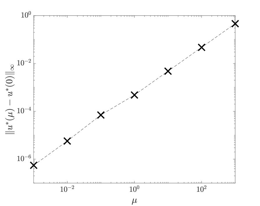
Figure 1: Difference between $u^{*}(\mu)$ and $u^{*}(0)$ in [kW].

We consider a benchmark case study from (Bitlislioğlu et al. (2017)) with a mix of $12$ commercial buildings including $2$ Large, $7$ Middle and $3$ Small such that there are $1456$ variables and $4816$ affine inequality constraints in total. Regarding the choice of $\mu$, Fig. 1 illustrates the difference between the optimal solutions of (18) with different $\mu\neq 0$ and the result with $\mu=0$. The gap $\|u^{*}(\mu)-u^{*}(0)\|_{\infty}$ increases linearly with $\mu$ increasing. We set the accuracy of the online solver as $10^{-4}$ such that we choose $\mu=10^{-1}$ in our implementation.

Fig. 2 and Fig. 3 show the convergence comparison between ALADIN and ADMM for two different online cases. In the first one, the optimal active set is almost the same as the previous MPC iteration. On the contrary, there are some changes of the optimal active set arising in the second case.

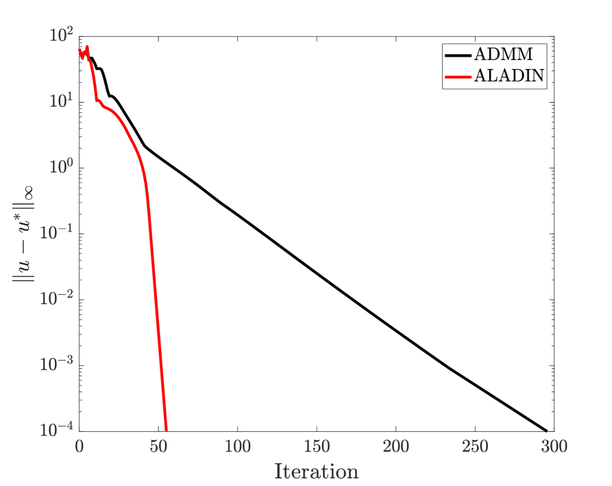
Figure 2: Convergence comparison of Case I: ALADIN vs ADMM.

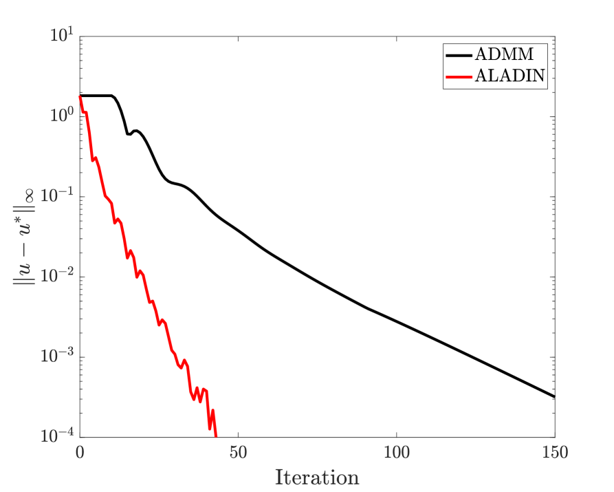
Figure 3: Convergence comparison of Case II: ALADIN vs ADMM.

Fig. 2 shows the comparison of an example of the first case. For solving this particular problem, when we set the tolerance to $10^{-4}$, ALADIN is five times faster than ADMM. In this case study, $252$ constraints are active at the optimal solution. The warm-start strategy for initializing $\Sigma_{i}$ improves the local convergence of ALADIN. Fig. 3 shows a comparison for the second case. In this example, $42$ constraints are active at the optimal solution. ALADIN just achieves a global linear convergence and is only three times faster than ADMM.

5 Conclusion

This paper analyzed an optimization problem for coordinating multiple commercial buildings. The problem balances the voltage surge of the building network by using an energy cost defined demand response criterion. By introducing an auxiliary variable, the problem was reformulated into a standard distributed form with decoupled PWQ objectives and coupled affine equality constraints. For solving this non-smooth convex problem in an MPC scheme, we proposed a tailored ALADIN method, which can warmly start online and thus its convergence can be sped up. Our numerical results illustrated the effectiveness of the warm-start strategy and show that the ALADIN based MPC controller outperforms the ADMM based controller.

References

- Alessio and Bemporad (2009) Alessio, A. and Bemporad, A. (2009). A survey on explicit model predictive control. In Nonlinear model predictive control, 345–369. Springer.
- Bitlislioglu (2018) Bitlislioglu, A. (2018). Coordinated optimization and control for smart grids. Technical report, Ecole Polytechnique Fédérale de Lausanne (EPFL).
- Bitlislioğlu et al. (2017) Bitlislioğlu, A., Pejcic, I., and Jones, C.N. (2017). Interior point decomposition for multi-agent optimization. IFAC-PapersOnLine, 50(1), 233–238.
- Bitlislioğlu and Jones (2017) Bitlislioğlu, A. and Jones, C.N. (2017). On coordinated primal-dual interior-point methods for multi-agent optimization. In 2017 IEEE 56th Annual Conference on Decision and Control (CDC), 3531–3536.
- Borrelli et al. (2003) Borrelli, F., Bemporad, A., and Morari, M. (2003). Geometric algorithm for multiparametric linear programming. Journal of optimization theory and applications, 118(3), 515–540.
- Boyd et al. (2011) Boyd, S., Parikh, N., Chu, E., Peleato, B., and Eckstein, J. (2011). Distributed optimization and statistical learning via the alternating direction method of multipliers. Foundations and Trends in Machine learning, 3(1), 1–122.
- Boyd and Vandenberghe (2004) Boyd, S. and Vandenberghe, L. (2004). Convex optimization. Cambridge University Press.
- Braun et al. (2018) Braun, P., Faulwasser, T., Grüne, L., Kellett, C.M., Weller, S.R., and Worthmann, K. (2018). Hierarchical distributed ADMM for predictive control with applications in power networks. IFAC Journal of Systems and Control, 3, 10–22.
- Crawley et al. (2000) Crawley, D.B., Pedersen, C.O., Lawrie, L.K., and Winkelmann, F.C. (2000). Energyplus: Energy simulation program. ASHRAE Journal, 42, 49–56.
- Engelmann et al. (2019) Engelmann, A., Jiang, Y., Houska, B., and Faulwasser, T. (2019). Towards distributed OPF using ALADIN. IEEE Transactions on Power Systems, 34(1), 584–594.
- Frasch et al. (2015) Frasch, J.V., Sager, S., and Diehl, M. (2015). A parallel quadratic programming method for dynamic optimization problems. Mathematical Programming Computation, 7(3), 289–329.
- Goldstein et al. (2014) Goldstein, T., O’Donoghue, B., Setzer, S., and Baraniuk, R. (2014). Fast alternating direction optimization methods. SIAM Journal on Imaging Sciences, 7(3), 1588–1623.
- Gorecki et al. (2015) Gorecki, T., Qureshi, F., and Jones, C.N. (2015). Openbuild : An integrated simulation environment for building control. In 2015 IEEE Conference on Control Applications (CCA), 1522–1527.
- Hong and Luo (2017) Hong, M. and Luo, Z. (2017). On the linear convergence of the alternating direction method of multipliers. Mathematical Programming, 162(1-2), 165–199.
- Houska et al. (2016) Houska, B., Frasch, J., and Diehl, M. (2016). An augmented Lagrangian based algorithm for distributed nonconvex optimization. SIAM Journal on Optimization, 26(2), 1101–1127.
- Jiang et al. (2019) Jiang, Y., Oravec, J., Houska, B., and Kvasnica, M. (2019). Parallel explicit model predictive control. arXiv preprint arXiv:1903.06790.
- Jiang et al. (2017) Jiang, Y., Zanon, M., Hult, R., and Houska, B. (2017). Distributed algorithm for optimal vehicle coordination at traffic intersections. In In Proceedings of the 20th IFAC World Congress, Toulouse, France, 12082–12087.
- Liserre et al. (2010) Liserre, M., Sauter, T., and Hung, J.Y. (2010). Future energy systems: Integrating renewable energy sources into the smart power grid through industrial electronics. IEEE industrial electronics magazine, 4(1), 18–37.
- O’Donoghue et al. (2016) O’Donoghue, B., Chu, E., Parikh, N., and Boyd, S. (2016). Conic optimization via operator splitting and homogeneous self-dual embedding. Journal of Optimization Theory and Applications, 169(3), 1042–1068.
- Oldewurtel et al. (2012) Oldewurtel, F., Parisio, A., Jones, C.N., Gyalistras, D., Gwerder, M., Stauch, V., Lehmann, B., and Morari, M. (2012). Use of model predictive control and weather forecasts for energy efficient building climate control. Energy and Buildings, 45, 15–27.
- Rantzer (2009) Rantzer, A. (2009). Dynamic dual decomposition for distributed control. In 2009 American Control Conference, 884–888. IEEE.
- Rawlings et al. (2017) Rawlings, J., Mayne, D.Q., and Diehl, M. (2017). Model Predictive Control: Theory, Computation, and Design. Nob Hill Publishing.
- Richter et al. (2011) Richter, S., Morari, M., and Jones, C.N. (2011). Towards computational complexity certification for constrained MPC based on Lagrange relaxation and the fast gradient method. In 2011 50th IEEE Conference on Decision and Control and European Control Conference, 5223–5229. IEEE.
- Ruiz (2001) Ruiz, D. (2001). A scaling algorithm to equilibrate both rows and columns norms in matrices. Technical report, Rutherford Appleton Laboratorie.
- Siano (2014) Siano, P. (2014). Demand response and smart grids—a survey. Renewable and sustainable energy reviews, 30, 461–478.