Analyticity, renormalization, and evolution
of the soft-quark function

Abstract

We compute the renormalization and evolution of the soft-quark function that appears in the factorization theorem for Higgs-boson decays to two photons through a $b$-quark loop. Our computation confirms a conjecture by Liu, Mecaj, Neubert, Wang, and Fleming for the form of the renormalization and evolution of the soft-quark function in order $\alpha_{s}$. We also work out the analyticity structure of the soft-quark function by making use of light-cone perturbation theory.

I Introduction

One of the principal decay modes of the Higgs boson is the decay to two photons ($H\to\gamma\gamma$). Comparison of the theoretical prediction for the rate of this decay mode with experimental measurements provides an important test of the standard model, and improvements in the precision of the theoretical prediction can lead to increasingly stringent tests.

One mechanism for this decay mode proceeds through the coupling of the Higgs boson to a virtual $b$-quark loop, which, in turn, couples to the final-state photons (Fig. 1). While this is not the dominant mechanism in $H\to\gamma\gamma$ decays, it is relevant to precision calculations of the decay rate. Furthermore, as we will explain, it is of particular theoretical interest.

Perturbative-QCD corrections to $H\to\gamma\gamma$ through a $b$-quark loop contain logarithms of $m_{H}^{2}/m_{b}^{2}$ Spira:1995rr , where $m_{H}$ and $m_{b}$ are the Higgs-boson and $b$-quark masses, respectively. Resummation of these large logarithms is essential to a well-controlled theoretical prediction. A traditional approach to resummation would be to make use of the $b\bar{b}$ light-cone distribution amplitudes for the photon. However, such an approach fails in this case because the amplitude for the decay process is proportional to $m_{b}$ at the leading nontrivial order in $m_{b}/m_{H}$. As is well known, such helicity-flip processes contain endpoint singularities that arise when all of the momentum of a spectator $b$ quark or antiquark is transferred to an active $b$ quark or antiquark. The endpoint singularities result in ill-defined quantities when one attempts to apply traditional resummation methods.

The endpoint singularities for exclusive amplitudes involving heavy quarks have been known for some time Beneke:2000ry ; Beneke:2001at ; Beneke:2001ev ; Beneke:2003pa ; Beneke:2003zv ; Jia:2010fw ; Benzke:2010js . They are associated with amplitudes that are suppressed by a power of the large momentum transfer and correspond to a pinch-singular region in momentum space in which the heavy quark carries a soft momentum Bodwin:2014dqa . Making use of this insight, the authors of Ref. Liu:2019oav have proposed a factorization theorem for $H\to\gamma\gamma$ through a $b$-quark loop that decomposes the endpoint contributions into the convolution of a soft-quark function with jet functions that account for contributions that arise from collinear quarks and gluons. In this factorization theorem, the endpoint contributions are well defined, and it can be used to resum logarithms of $m_{H}^{2}/m_{b}^{2}$. A similar factorization theorem has been proposed in Ref. Wang:2019mym . The renormalized form of the factorization theorem has been given in Refs. Liu:2020tzd ; Liu:2020wbn . The factorization theorem is stated in the language of soft-collinear effective theory (SCET) Bauer:2000yr ; Bauer:2001yt ; Beneke:2002ni ; Bauer:2002nz ; Beneke:2002ph .

As we have mentioned, one of the elements of the factorization theorem is a soft-quark function. (Hereinafter, we refer to it as the “soft function.”) Its renormalization-group evolution equation is an essential component in the resummation of logarithms of $m_{H}^{2}/m_{b}^{2}$, and can be derived, to a given order in $\alpha_{s}$, once one has worked out the renormalization condition for the soft function to that order in $\alpha_{s}$.

Note that, in order to derive the evolution equation, one must work out the renormalization condition for a generic soft function. In deriving the evolution equation, it is not sufficient to compute the UV divergences of the fixed-order (in $\alpha_{s}$) soft function, because the renormalization condition for the soft function involves a convolution of the renormalization factor with the soft function, rather than a simple multiplication. One must make the convolution integrals explicit in order to deduce the renormalization condition.

In Ref. Liu:2019oav , the soft function was computed at order-$\alpha_{s}$, and the UV poles in dimensional regularization were identified. However, as we have mentioned, such a calculation is insufficient to work out the evolution equation for the soft function.

In Ref. Liu:2020eqe , a conjecture was given for the renormalization/evolution of the soft function through order $\alpha_{s}^{2}$. In that work, the renormalization condition for the soft function was derived by assuming the consistency condition, which implies the renormalization-group invariance of the so-called “soft sector” of the factorization theorem, which consists of the product of a certain Wilson coefficient with the convolution of the soft function with radiative jet functions Liu:2019oav . However, the renormalization-group invariance of the soft sector has not been established, and, indeed, in Ref. Liu:2019oav , it is pointed out that the renormalization-group invariance is violated at one-loop level once one has imposed rapidity regulators that are needed to make the convolution integral in the soft sector well defined. The conjecture for the evolution equation for the soft function is also stated, without further explanation, in Ref. Liu:2020wbn

Given the importance of the soft function in the factorization/resummation program, it is essential to put the renormalization condition for the soft function on a more solid footing. In the present paper, we work out the renormalization/evolution of the soft function through order $\alpha_{s}$. Our computation confirms the conjecture in Ref. Liu:2020eqe through order $\alpha_{s}$. The analysis is novel because, as we will explain in detail, the momentum routing in the soft function is unorthodox: The various components of the loop momenta route through different propagators and vertices. This unorthodox momentum arises as a consequence of the factorization of the soft function from the radiative jet functions. It results in some unexpected analyticity properties of the soft function. It also leads to a nonlocal renormalization condition for the soft function, although, as is well known, nonlocal renormalization conditions can also appear in the case of standard momentum routing, for example, in the renormalization of parton distributions.

Our calculation relies on the analytic structure of the soft function in the complex plane of its longitudinal-momentum variables. In Ref. Liu:2019oav , the analyticity properties of the soft function were asserted. In the present paper, we establish those properties by showing how the regions of non-analyticity arise in specific examples and by giving a general argument for the analyticity everywhere else in the complex plane. Our arguments make use of light-front perturbation theory.

The remainder of this paper is organized as follows. In Sec. II, we define some of our notation. Section III contains a statement of the factorization theorem for $H\to\gamma\gamma$ through a $b$-quark loop. In Sec. IV we give the operator definition of the soft function, and in Sec. V we give its decomposition into structure functions and define its discontinuity. We present the diagrammatic form of the soft function in Sec. VI, discuss the leading-order (LO) and next-to-leading order (NLO) contributions to the soft function in Sec. VII, and examine the analyticity of the soft function in Sec. VIII. Examples that illustrate the analyticity structure of the soft function and details of the general analyticity argument are given in the Appendix. Sec. IX contains a general discussion of the renormalization of the soft function. In Sec. X, we present our calculation of the one-loop renormalization of the soft function and write down the evolution equation for the particular structure function that appears in the process $H\to\gamma\gamma$. Finally, we summarize our results in Sec. XI.

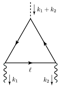
Figure 1: $H\rightarrow b\bar{b}\rightarrow\gamma\gamma$ at leading order. The dashed line represents the Higgs boson, the solid line represents the $b$ quark, and the wavy lines are the photons.

II Notation and conventions

In this section, we establish some of our notation and conventions, which generally agree with those that are used in Ref. Liu:2019oav .

In Fig. 1 we show the LO Feynman diagram for the decay $H\to\gamma\gamma$ through a $b$-quark loop. The final-state photons have light-like momenta $k_{1}$ and $k_{2}$. We define two light-like vectors, $n_{1}$ and $n_{2}$, that are collinear to $k_{1}$ and $k_{2}$, respectively. They satisfy the conditions

$$n_{1}^{2}=0,\qquad n_{2}^{2}=0,\qquad n_{1}\cdot n_{2}=2.$$ (1)

Then, any four vector $\ell$ can be decomposed as

$$\ell^{\mu}=(n_{1}\cdot\ell)\frac{n_{2}^{\mu}}{2}+(n_{2}\cdot\ell)\frac{n_{1}^{\mu}}{2}+\ell_{\perp}^{\mu}=\ell_{+}\frac{n_{2}^{\mu}}{2}+\ell_{-}\frac{n_{1}^{\mu}}{2}+\ell_{\perp}^{\mu},$$ (2)

where $\ell_{\perp}^{\mu}=(0,\ell^{1},\ell^{2},0)$ and we have defined

$$\ell_{+}\equiv n_{1}\cdot\ell,\quad\ell_{-}\equiv n_{2}\cdot\ell.$$ (3)

Consequently, the scalar product of two momenta is given by

$$k\cdot\ell = \frac{k_{+}\ell_{-}}{2}+\frac{k_{-}\ell_{+}}{2}+k_{\perp}\cdot\ell_{\perp}=\frac{k_{+}\ell_{-}}{2}+\frac{k_{-}\ell_{+}}{2}-\bm{k}_{\perp}\cdot\bm{\ell}_{\perp},$$ (4)

where $\bm{\ell}_{\perp}$ and $\bm{k}_{\perp}$ are Euclidean two-vectors.

III Factorization theorem

A factorization formula for the amplitude for $H\to\gamma\gamma$ through $b$-quark loop is given in Ref. Liu:2019oav . It holds up to corrections of relative order $m_{b}/m_{H}$ and can be written as

$$\mathcal{M}_{b}(H\to\gamma\gamma)=\sum_{i=1}^{3}H_{i}\langle\gamma\gamma|{\cal O}_{i}|H\rangle,$$ (5)

where the ${\cal O}_{i}$ are operators that are defined in Ref. Liu:2019oav , the $H_{i}$ are hard matching coefficients (Wilson coefficients), and the products of the $H_{i}$ and the operator matrix elements are in the convolutional sense. ${\cal O}_{1}$ is a contact interaction between the Higgs and photon fields. ${\cal O}_{2}$ is a sum of two contributions, one involving the photon with momentum $k_{1}$ and the corresponding SCET collinear field and the other involving the photon with momentum $k_{2}$ and the corresponding SCET collinear field. ${\cal O}_{3}$ involves hard-collinear SCET fields for both the $k_{1}$ and $k_{2}$ directions and a soft-quark field. Explicit expressions for these operator matrix elements and graphical representations of them are given in Ref. Liu:2019oav .

After applying the field redefinitions Bauer:2001yt which decouple the hard-collinear fields from the soft gluons, one can write the factorized form of ${\cal O}_{3}$ as follows Liu:2019oav :

$${\cal O}_{3} = H(0)\int d^{D}x\int d^{D}y\,T\bigg{\{}\left[\left(\mathcal{A}\!\!\!/^{\perp}_{n_{1}}(x)+\mathcal{G}\!\!\!/^{\perp}_{n_{1}}(x)\right)\mathcal{X}_{n_{1}}(x)\right]^{\alpha i}\bar{\mathcal{X}}^{\beta j}_{n_{1}}(0)\bigg{\}}$$ (6)

$$\times T\bigg{\{}\mathcal{X}^{\beta k}_{n_{2}}(0)\left[\bar{\mathcal{X}}_{n_{2}}(y)\left(\mathcal{A}\!\!\!/^{\perp}_{n_{2}}(y)+\mathcal{G}\!\!\!/^{\perp}_{n_{2}}(y)\right)\right]^{\gamma l}\bigg{\}}$$

$$\times T\bigg{\{}\left[S^{\dagger}_{n_{2}}(y_{+})q_{s}(y_{+})\right]^{\gamma l}\left[\bar{q}_{s}(x_{-})S_{n_{1}}(x_{-})\right]^{\alpha i}\left[S^{\dagger}_{n_{1}}(0)S_{n_{2}}(0)\right]^{jk}\bigg{\}}+\textrm{h.c.},$$

where h.c. denotes the hermitian conjugate contributions, $T$ denotes a time-ordered product, and $(i,j,k,l)$ and $(\alpha,\beta,\gamma)$ are color and spin indices, respectively. $H$ is the Higgs-boson field, and $q_{s}$ is the soft-quark SCET field. $\mathcal{A}^{\mu}_{n_{i}}$, $\mathcal{G}^{\mu}_{n_{i}}$, and $\mathcal{X}_{n_{i}}$ are the building blocks of SCET for the $n_{i}$-hard-collinear photon, gluon, and quark fields, respectively. The $S_{n_{i}}$ are soft Wilson lines (in distinction to the collinear Wilson lines, which are contained in the $\mathcal{X}_{n_{i}}$), which are defined by

$$S_{n_{i}}(x) = P~{}\text{exp}\left[ig_{s}\int_{-\infty}^{0}dt~{}n_{i}\cdot G_{s}(x+tn_{i})\right].$$ (7)

Here, $G_{s}$ is the soft-gluon field.

In Eq. (6), the first and second time-ordered products are the jet operators that account for the contributions that are collinear to $n_{1}$ and $n_{2}$, respectively, and the last time-ordered product is the soft operator. In Ref. Liu:2020eqe , the authors take matrix elements of the jet operators between the vacuum and one-photon states, take the vacuum-to-vacuum matrix element of the soft operator, take Fourier transforms of these matrix elements, extract some kinematic and Dirac-matrix factors, and make use of analyticity properties of the matrix elements to arrive at a factorized form for $\langle\gamma\gamma|{\cal O}_{3}|H\rangle$ that depends only on scalar jet and soft functions:

$$\langle\gamma\gamma|{\cal O}_{3}|H\rangle=2g_{\perp}^{\mu\nu}\int_{0}^{\infty}\frac{d\omega}{\omega}S_{1}(\omega)\int_{\sqrt{\omega}}^{\infty}\frac{d\ell_{-}}{\ell_{-}}J(m_{H}\omega/\ell_{-})J(-m_{H}\ell_{-}).$$ (8)

Here, $\omega=\ell_{+}\ell_{-}$, $S_{1}(\omega)$ is the discontinuity of a structure function of the soft function, which we define in Eq. (17) below, and $J$ is the radiative jet function DelDuca:1990gz ; Bonocore:2015esa ; Bonocore:2016awd which describes the emission of collinear gluons from a collinear $b$ quark. The radiative jet function also appears in the radiative $B$-meson decay $B^{-}\to\gamma\ell^{-}\bar{\nu}$ Lunghi:2002ju ; Bosch:2003fc ; Wang:2016qii ; Wang:2018wfj . The integrations in Eq. (8) contain rapidity divergences as $\omega$ and $\ell_{-}$ tend to infinity and are well defined only after one has imposed a rapidity regulator or a cutoff Liu:2020eqe .

IV Operator definition of the soft function

Following Ref. Liu:2020eqe , we define the soft function in terms of a vacuum-to-vacuum matrix element of the product of the soft-quark propagator with soft Wilson lines:

$$\bm{S}(\ell_{+},\ell_{-}) = \frac{2i\pi}{N_{c}}\int dx_{-}dy_{+}\exp\left[i\frac{\ell_{-}y_{+}-\ell_{+}x_{-}}{2}\right]$$

$$\times\langle 0|T\,\text{Tr}\biggl{[}S_{n_{2}}(0)S^{\dagger}_{n_{2}}(y_{+},0,\bm{0}_{\perp})q_{s}(y_{+},0,\bm{0}_{\perp})\bar{q}_{s}(0,x_{-},\bm{0}_{\perp})S_{n_{1}}(0,x_{-},\bm{0}_{\perp})S^{\dagger}_{n_{1}}(0)\biggr{]}|0\rangle.$$

Here, $N_{c}=3$ is the number of quark colors, and the trace is over color, but not spinor, indices. The products of semi-infinite Wilson lines $S_{n_{i}}S_{n_{i}}^{\dagger}$ in Eq. (IV) can be written as finite-length Wilson lines Liu:2020eqe . We find it more convenient in our calculations to keep the Wilson lines in the product form. However, one should bear in mind that, because the product of semi-infinite Wilson lines yields a Wilson line of finite length, the rapidity divergences that are associated with the individual semi-infinite Wilson lines cancel.

The expression for the soft function contains an implicit integration over the transverse momentum of the soft quark. It is convenient to make this integration manifest, which we accomplish by defining an unintegrated soft function

$$\bm{S}(\ell_{+},\ell_{-},\ell_{\perp}) = \frac{2i\pi}{N_{c}}\int dx_{-}dy_{+}d^{D-2}\bm{z}_{\perp}\exp\left[i\left(\frac{\ell_{-}y_{+}-\ell_{+}x_{-}}{2}-\bm{\ell}_{\perp}\cdot\bm{z}_{\perp}\right)\right]$$ (10)

$$\times\langle 0|T\,\text{Tr}\biggl{[}S_{n_{2}}(0,0,\bm{z}_{\perp}/2)S^{\dagger}_{n_{2}}(y_{+},0,\bm{z}_{\perp}/2)q_{s}(y_{+},0,\bm{z}_{\perp}/2)$$

$$\quad~{}\times\bar{q}_{s}(0,x_{-},-\bm{z}_{\perp}/2)S_{n_{1}}(0,x_{-},-\bm{z}_{\perp}/2)S^{\dagger}_{n_{1}}(0,0,-\bm{z}_{\perp}/2)\biggr{]}|0\rangle,$$

where

$$\int_{\bm{\ell}_{\perp}}\bm{S}(\ell_{+},\ell_{-},\ell_{\perp}) = \bm{S}(\ell_{+},\ell_{-}),$$ (11)

with

$$\int_{\bm{\ell}_{\perp}} \equiv \int\frac{d^{D-2}\bm{\ell}_{\perp}}{(2\pi)^{D-2}},$$ (12)

where the number of space-time dimensions $D=4-2\epsilon$ is used to regularize divergent integrals.

V Structure functions and discontinuities

We wish to decompose the soft function into structure functions. The reparametrization invariance of the soft function requires that any numerator factor $n_{1}$ ($n_{2}$) be accompanied by a denominator factor $n_{1}$ ($n_{2}$) Manohar:2002fd ; Liu:2020eqe . (We use $n_{1}\cdot n_{2}=2$ to eliminate factors $n_{1}\cdot n_{2}$.) Then we can decompose the unintegrated soft function $\bm{S}(\ell_{+},\ell_{-},{\ell}_{\perp})$ as follows:

$$\bm{S}(\ell_{+},\ell_{-},\ell_{\perp}) = m_{b}\bm{S}_{1}(\omega,\bm{\ell}_{\perp}^{2})+\frac{\not{n}_{1}}{2}(n_{2}\cdot\ell)\bm{S}_{2}(\omega,\bm{\ell}_{\perp}^{2})+\frac{\not{n}_{2}}{2}(n_{1}\cdot\ell)\bm{S}_{3}(\omega,\bm{\ell}_{\perp}^{2})+m_{b}\frac{\not{n}_{2}\not{n}_{1}}{4}\bm{S}_{4}(\omega,\bm{\ell}_{\perp}^{2})$$

$$+\not{\ell}_{\perp}\bm{S}_{5}(\omega,\bm{\ell}_{\perp}^{2})+\frac{m_{b}\not{n}_{1}\not{\ell}_{\perp}}{2(n_{1}\cdot\ell)}\bm{S}_{6}(\omega,\bm{\ell}_{\perp}^{2})+\frac{m_{b}\not{\ell}_{\perp}\not{n}_{2}}{2(n_{2}\cdot\ell)}\bm{S}_{7}(\omega,\bm{\ell}_{\perp}^{2})+\frac{\not{n}_{2}\not{\ell}_{\perp}\not{n}_{1}}{4}\bm{S}_{8}(\omega,\bm{\ell}_{\perp}^{2}),$$

where the structure functions $\bm{S}_{i}$ are scalar-valued functions of $\omega=\ell_{+}\ell_{-}$ and $\bm{\ell}_{\perp}^{2}$. The Dirac structures are the most general parity-even ones that can be obtained from the four-vectors $\ell$, $n_{1}$, and $n_{2}$, subject to the reparametrization-invariance constraints. In selecting this particular decomposition into linearly independent Dirac structures, we have observed the convention that $\not{n}_{1}$ always appears to the right of $\not{n}_{2}$. This will prove to be convenient when we take into account the Dirac structure of the jet and hard factors in the factorization theorem. The decomposition of the integrated soft function into structure functions is given by

$$\bm{S}(\ell_{+},\ell_{-}) = m_{b}\bm{S}_{1}(\omega)+\frac{\not{n}_{1}}{2}(n_{2}\cdot\ell)\bm{S}_{2}(\omega)+\frac{\not{n}_{2}}{2}(n_{1}\cdot\ell)\bm{S}_{3}(\omega)+m_{b}\frac{\not{n}_{2}\not{n}_{1}}{4}\bm{S}_{4}(\omega),$$ (14)

where the integrated form factors are defined by

$$\bm{S}_{i}(\omega)=\int_{\bm{\ell}_{\perp}}\bm{S}_{i}(\omega,\bm{\ell}_{\perp}^{2}),\quad\textrm{for $i=$1, 2, 3, and 4.}$$ (15)

Note that the $\ell_{\perp}$-dependent contributions are now absent in the decomposition of the integrated soft function.

It is shown in Ref. Liu:2020eqe that, because of the analytic properties of the soft function (see Sec. VIII) and the jet functions, the factorization theorem for $H\to\gamma\gamma$ through a $b$-quark loop can be written in terms of the discontinuity of the soft function, which is given by

$$S(\omega) = \frac{1}{2\pi i}[\bm{S}(\omega+i\varepsilon)-\bm{S}(\omega-i\varepsilon)].$$ (16)

We use a non-bold $S$ to distinguish the discontinuity of the soft function from the soft function $\bm{S}$. Similarly, we use $S_{i}$ to denote the discontinuities of the soft structure functions $\bm{S}_{i}$:

$$S_{i}(\omega) = \frac{1}{2\pi i}[\bm{S}_{i}(\omega+i\varepsilon)-\bm{S}_{i}(\omega-i\varepsilon)].$$ (17)

VI Diagrammatic form of the soft function

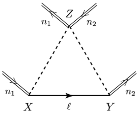
Figure 2: Diagrammatic form of the integrated soft function $\bm{S}(\ell_{+},\ell_{-})$. The solid line is a soft-quark propagator. The double solid lines with incoming arrows are Wilson lines $S_{n_{i}}$, and the double solid lines with outgoing arrows are hermitian-conjugate Wilson lines $S_{n_{i}}^{\dagger}$. The dashed lines indicate a space-time separation, as is described in the text.

The diagrammatic form of the integrated soft function $\bm{S}(\ell_{+},\ell_{-})$ is shown in Fig. 2. For clarity, we have suppressed gluons, which attach in all possible ways to the Wilson lines and the soft-quark propagator. The gluons interact with themselves, Wilson lines, soft-quarks, light-quarks, and ghosts according to the standard rules of QCD. The Feynman rules for a Wilson line that is collinear to $n_{i}$ follow from the definition in Eq. (7). They are given in Fig. 3.

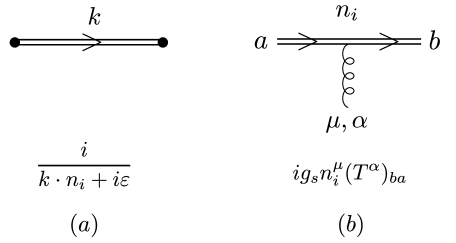
Figure 3: Feynman rules for a Wilson line $S_{n_{i}}$ that is collinear to $n_{i}$. (a) The Wilson-line propagator. (b) The vertex for the interaction of a gluon with the Wilson line. $a$ and $b$ are color indices and $T^{\alpha}$ is the SU(3) generating matrix for the fundamental representation. These rules apply to a diagrammatic Wilson line for which the arrow is incoming to a vertex. A diagrammatic Wilson line for which the arrow is outgoing from a vertex denotes a hermitian-conjugate Wilson line $S_{n_{i}}^{\dagger}$. One obtains the Feynman rules for $S_{n_{i}}^{\dagger}$ from the rules in the figure by taking the hermitian conjugate.

The dashed lines in Fig. 2 are not propagators but, rather, indicate a space-time separation. There is no separation in the transverse direction between the points $X$ and $Z$ and between the points $Y$ and $Z$. Hence, transverse momenta can be routed between the points $X$ and $Z$ and between the points $Y$ and $Z$. The points $X$ and $Z$ are separated in the $-$ light-front direction, but not in the $+$ light-front direction. [That is, $n_{2}\cdot(X-Z)=(X-Z)_{-}\neq 0$, but $n_{1}\cdot(X-Z)=(X-Z)_{+}=0$.] Similarly, the points $Y$ and $Z$ are separated in the $+$ light-front direction, but not in the $-$ light-front direction. Hence, $-$ components of momentum can be routed between $X$ and $Z$, and $+$ components of momentum can be routed between $Y$ and $Z$. The external momentum $\ell_{+}$ enters the diagram at $X$, proceeds through the soft-quark propagator to $Y$, and then proceeds to $Z$, which is a sink. Similarly, the external momentum $-\ell_{-}$ enters the diagram at $Y$, proceeds through the soft-quark propagator to $X$, and then proceeds to $Z$. The internal momentum $\ell_{\perp}$ runs in a loop from $X$ to $Y$ to $Z$ to $X$.

It is easy to understand the form of the soft function in terms of a diagrammatic analysis in QCD. In the factorization formula in Eq. (5), the pinch-singular contributions to the operator matrix element $\langle\gamma\gamma|{\cal O}_{3}|H\rangle$ come from a region of momentum space in which the left-hand quark line in Fig. 1 and associated gluons comprise a jet in which all of the particles are collinear to $k_{1}$, the right-hand quark line in Fig. 1 and associated gluons comprise a jet in which all of the particles are collinear to $k_{2}$, and the lower quark line and associated gluons form a subgraph in which all of particles are soft. Gluons from the soft subgraph can attach to particles in either of the jets.

One can follow standard procedures to factor these gluons topologically from the jets. (See, for example, Ref. Collins:1989gx .) First, one makes the appropriate soft approximation (Grammer-Yennie approximation Grammer:1973db ) for the soft-gluon attachments to each jet. Then one applies graphical Ward identities to factor the gluon attachments. This produces a Wilson line $S_{n_{1}}$ at the lower end of the $k_{1}$ jet, a Wilson line $S_{n_{1}}^{\dagger}$ at the upper end of the $k_{1}$ jet, a Wilson line $S_{n_{2}}^{\dagger}$ at the lower end of the $k_{2}$ jet, and a Wilson line $S_{n_{2}}$ at the upper end of the $k_{2}$ jet. The Wilson lines at the upper ends of the jets still appear to entangle the soft gluons with the jets. However, that entanglement can be removed by making use of the facts that the $k_{1}$ jet is sensitive only to the $+$ components of momenta that are routed through it and the $k_{2}$ jet is sensitive only to the $-$ components of momenta that are routed through it. Then, one can route the $+$ components of the momenta of gluons that attach to $S_{n_{1}}^{\dagger}$ through the $k_{2}$ jet and route the $-$ components of the momenta of gluons that attach to $S_{n_{2}}$ through the $k_{1}$ jet, thereby rendering the jet functions insensitive to the gluon momenta in the upper Wilson lines. This unorthodox momentum routing results in the factorization of the soft function from the jet functions and leads to the space-time picture in Fig. 2.

As we will see, the unorthodox flow of momenta in the soft function results in a nonlocal UV renormalization of the soft function.

VII LO and NLO contributions to the soft function

The LO soft function is given by the integral of the soft-quark propagator over $\ell_{\perp}$:

$$\bm{S}^{\text{LO}}(\ell_{+},\ell_{-}) = m_{b}\bm{S}^{\text{LO}}_{1}(\omega)+\frac{\not{n}_{1}}{2}\,n_{2}\cdot\ell\,\bm{S}^{\text{LO}}_{2}(\omega)+\frac{\not{n}_{2}}{2}\,n_{1}\cdot\ell\,\bm{S}^{\text{LO}}_{3}(\omega),$$ (18)

where the LO structure functions are

$$\bm{S}^{\text{LO}}_{1,2,3}(\omega) = (4\pi)^{\epsilon}\Gamma(\epsilon)\left(-\omega+m_{b}^{2}-i\varepsilon\right)^{-\epsilon}.$$ (19)

The discontinuities of the LO soft structure functions are

$$S^{\text{LO}}_{1,2,3}(\omega) = \frac{(4\pi)^{\epsilon}}{\Gamma(1-\epsilon)}\left(\omega-m_{b}^{2}\right)^{-\epsilon}\theta(\omega-m_{b}^{2})=\theta(\omega-m_{b}^{2})\left[1+O(\epsilon)\right].$$ (20)

Expressions for the NLO soft function are given in Eqs. (4.6)–(4.8) and (B.1) of Ref. Liu:2019oav . We have confirmed these expressions.

VIII Analyticity of the soft function

In Ref. Liu:2020eqe , it is stated that the soft function $\bm{S}(\ell_{+},\ell_{-})$ is analytic in the complex $\omega$ plane, except for a cut that lies just below the positive real axis and extends from $\omega=-i\varepsilon$ to infinity. This is somewhat surprising, as one might expect the cut to extend from the threshold for production of the massive bottom quark, $\omega=m_{b}^{2}$, to infinity. This is indeed the case for the lowest-order contribution to $\bm{S}(\ell_{+},\ell_{-})$. However, as we show through some specific one-loop examples in Appendix A, a cut does indeed appear along the entire $\omega$ positive real axis. The examples are presented in terms of $x_{+}$-ordered light-front perturbation theory.

The analyticity of the soft function is described by the analyticity of its structure functions. As we have seen, the structure functions are functions of the product $\ell_{+}\ell_{-}$. Therefore, in considering the analyticity of the structure functions as a function of $\omega=\ell_{+}\ell_{-}$, we can, without loss of generality, take $\ell_{+}>0$. This choice simplifies the analysis of diagrams in light-front perturbation theory (see Appendix A) because it insures that the $+$ momentum of the initial soft-quark line is always positive (flowing from left to right in the light-front diagrams).

In light-front perturbation theory, imaginary contributions arise from vanishing energy denominators. This occurs when the initial light-front energy $\ell_{-}$ is equal to the sum of the on-shell light-front energies of the intermediate-state lines. An imaginary part can arise in some of the light-front diagrams when $\ell_{-}=\omega/\ell_{+}=0$ because the light-front energy of one of the on-shell intermediate states vanishes. This can happen because, in some light-front diagrams, a $b$-quark line can carry an infinite light-front longitudinal momentum $k_{+}$, causing its intermediate-state light-front energy $(\bm{k}_{\perp}^{2}+m_{b}^{2})/k_{+}$ to vanish. In an ordinary QCD $b$-quark-self-energy diagram, an infinite $+$ longitudinal momentum cannot appear in a $b$-quark line because it would result in a negative longitudinal momentum in one of the diagrammatic lines. Negative longitudinal momenta (backward-moving lines) are disallowed in light-front perturbation theory. However, in the soft function, owing to the unorthodox momentum routing or the presence of an $n_{2}$ Wilson line, a $b$-quark line in the soft function can carry infinite $+$ longitudinal momentum.

The property of light-front perturbation theory that all of the $+$ longitudinal momenta are positive insures that all of the light-front intermediate-state energies are also positive. Hence, the energy denominators can never vanish if $\ell_{-}<0$. For our choice $\ell_{+}>0$, this implies that the structure functions have no imaginary parts unless $\omega$ is greater than $0$. Therefore, we conclude that $\bm{S}(\ell_{+},\ell_{-})$ is analytic in the complex $\omega$ plane, except for a cut that runs just below the real axis from $\omega=-i\varepsilon$ to infinity.

IX Renormalization of the soft function

The soft-function structure functions are renormalized as

$$\bm{S}_{i}^{\textrm{R}}(\omega)=\sum_{j=1}\int_{0}^{\infty}d\omega^{\prime}Z_{S}^{ij}(\omega,\omega^{\prime};\mu)\bm{S}_{j}(\omega^{\prime}),$$ (21)

where ${\bm{S}}^{\textrm{R}}$ is the renormalized soft function and $\mu$ is the renormalization scale. As usual, $Z_{S}$ has an expansion in powers of the strong coupling $\alpha_{s}$:

$$Z_{S}=Z_{S}^{(0)}+\alpha_{s}Z_{S}^{(1)}+\alpha_{s}^{2}Z_{S}^{(2)}+\cdots.$$ (22)

In this paper, we compute $Z_{S}$ through order $\alpha_{s}$. The order-$\alpha_{s}$ contribution to $Z_{S}$ is the order-$\alpha_{s}$ counterterm for ${\bm{S}}$. In minimal subtraction in dimensional regularization, this is the negative of the UV pole terms that appear in the one-loop QCD corrections to ${\bm{S}}$.

Note that $Z_{S}$ contains only the renormalizations that are associated with ${\bm{S}}$ [renormalizations of the operator in Eq. (IV)] and does not include the coupling-constant and mass renormalizations of QCD. It does, however, include the wave-function renormalization that is associated with the soft-quark field.

In principle, the renormalization factor $Z_{S}$ includes a UV divergence that arises from the $\ell_{\perp}$ integration that is implicit in the definition of the soft operator. This divergence starts at order $\alpha_{s}^{0}$. [See Eq. (19).] We do not include this divergence in our computations of $Z_{S}$ because, ultimately, we are interested in the discontinuity of the soft function $S(\ell_{+},\ell_{-})$ [Eq. (16)]. In the discontinuity of the soft function, the $\ell_{\perp}$ integration does not produce a UV divergence because the discontinuity of the soft function has support over only a finite range of $\bm{\ell}_{\perp}^{2}$. The finiteness of the discontinuity of the LO soft function can be seen explicitly in Eq. (20).

In our calculations of the one-loop UV divergences in the soft function we include a factor of the all-orders soft function, along with the divergent loop. That is, we compute the one-loop counterterm corrections to the all-orders soft function. In using this method, it is essential to keep in mind that the all-orders soft function is factored from the one-loop contribution. That is, the loop momenta that are internal to the all-orders soft function do not enter into the one-loop expressions.

This method is advantageous for several reasons. First, as we have mentioned, the UV divergences in the soft function are nonlocal, in the sense that they involve integrations over the external longitudinal momenta of the soft function, rather than simple multiplications. We use the all-orders soft function to keep track of these integrations. Furthermore, as we will see, the UV divergences involve both left- and right-multiplication of the soft function by Dirac matrices. We use the all-orders soft function to keep track of these multiplications, as well. In addition, the explicit presence of the all-orders soft function allows us to make use of its analyticity properties to simplify the forms of the one-loop divergences.

X One-loop renormalization and evolution of the soft function

In this section, we compute the various contributions to the one-loop renormalization of the soft function. We denote the one-loop corrections, including a factor of the all-orders soft function, by $\bm{S}_{(i)}(\ell_{+},\ell_{-})$, where the subscript $i=A_{1},A_{2},A_{3},A_{4},B,C$ denotes the class of one-loop diagram.

X.1 Diagrams $\textbf{{A}}_{\textbf{{i}}}$

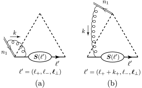
Figure 4: The diagrams that contribute to $\bm{S}_{(A_{1})}$. The blob represents the all-orders soft function. Its Wilson lines and the connections of gluons to them are suppressed.

The expression that corresponds to the diagrams that are shown in Fig. 4 is

$$\bm{S}_{(A_{1})}(\ell_{+},\ell_{-}) = ig_{s}^{2}C_{F}\left(\frac{\mu^{2}e^{\gamma_{E}}}{4\pi}\right)^{\epsilon}\int_{\bm{\ell}_{\perp}}\int\frac{dk_{+}dk_{-}d^{D-2}k_{\perp}}{(2\pi)^{D}}\frac{1}{(-k_{+}+i\varepsilon)(k^{2}+i\varepsilon)}$$ (23)

$$\times\Bigg{\{}-\frac{\bm{S}(\ell_{+},\ell_{-},\ell_{\perp})\frac{\not{n}_{1}}{2}\left[\frac{\not{n}_{2}}{2}\left(\ell_{+}-k_{+}\right)+\not{\ell}_{\perp}-\not{k}_{\perp}+m_{b}\right]}{(\ell_{+}-k_{+})(\ell_{-}-k_{-})-(\bm{\ell}_{\perp}-\bm{k}_{\perp})^{2}-m_{b}^{2}+i\varepsilon}$$

$$\quad~{}\,\,+\frac{\bm{S}(\ell_{+}+k_{+},\ell_{-},\ell_{\perp})\frac{\not{n}_{1}}{2}(\frac{\not{n}_{2}}{2}\ell_{+}+\not{\ell}_{\perp}-\not{k}_{\perp}+m_{b})}{\ell_{+}(\ell_{-}-k_{-})-(\bm{\ell}_{\perp}-\bm{k}_{\perp})^{2}-m_{b}^{2}+i\varepsilon}\Bigg{\}},$$

where the first term corresponds to the diagram in Fig. 4(a) and the second term corresponds to the diagram in Fig. 4(b). We have also made the integration over $k_{\perp}$ in the integrated soft function explicit. We note that there is a contribution that depends on $\bm{S}(\ell_{+}+k_{+},\ell_{-},\ell_{\perp})$, rather than on $\bm{S}(\ell_{+},\ell_{-},\ell_{\perp})$. This contribution arises because of the unorthodox momentum routing in the soft function, which is a consequence of the form of the factorization of the soft function from the jet functions. As we will see, such “nonlocal” contributions are a general feature of the renormalization of the soft function.

Let us initially consider the case $\ell_{+}>0$, $\ell_{-}<0$. We perform the $k_{-}$ integration by closing the contour in the lower half-plane and picking up the pole at $k_{-}=\frac{k_{\perp}^{2}}{k_{+}}-i\varepsilon$. This leads to

$$\bm{S}_{(A_{1})}(\ell_{+},\ell_{-}) = -2\alpha_{s}C_{F}\left(\frac{\mu^{2}e^{\gamma_{E}}}{4\pi}\right)^{\epsilon}\int_{\bm{\ell}_{\perp}}\int\frac{d^{D-2}k_{\perp}}{(2\pi)^{D-2}}\int_{0}^{\infty}\frac{dk_{+}}{k_{+}^{2}}$$ (24)

$$\times\Bigg{\{}-\frac{\theta(\ell_{+}-k_{+})\bm{S}(\ell_{+},\ell_{-},\ell_{\perp})\frac{\not{n}_{1}}{2}\left[\frac{\not{n}_{2}}{2}\left(\ell_{+}-k_{+}\right)+\not{\ell}_{\perp}-\not{k}_{\perp}+m_{b}\right]}{(\ell_{+}-k_{+})\ell_{-}-\frac{\ell_{+}-{k_{+}}}{k_{+}}\bm{k}_{\perp}^{2}-(\bm{\ell}_{\perp}-\bm{k}_{\perp})^{2}-m_{b}^{2}+i\varepsilon}$$

$$\quad~{}+\frac{\bm{S}(\ell_{+}+k_{+},\ell_{-},\ell_{\perp})\frac{\not{n}_{1}}{2}(\frac{\not{n}_{2}}{2}\ell_{+}+\not{\ell}_{\perp}-\not{k}_{\perp}+m_{b})}{\ell_{+}\ell_{-}-\frac{\ell_{+}}{k_{+}}\bm{k}_{\perp}^{2}-(\bm{\ell}_{\perp}-\bm{k}_{\perp})^{2}-m_{b}^{2}+i\varepsilon}\Bigg{\}}.$$

Translating the integration variable $k_{\perp}$ according to $k_{\perp}\rightarrow k_{\perp}+\frac{k_{+}}{\ell_{+}+k_{+}}\ell_{\perp}$ and $k_{\perp}\rightarrow k_{\perp}+\frac{k_{+}}{\ell_{+}}\ell_{\perp}$ for the first and second terms in the integrand, respectively, we obtain

$$\bm{S}_{(A_{1})}(\ell_{+},\ell_{-}) = 2\alpha_{s}C_{F}\left(\frac{\mu^{2}e^{\gamma_{E}}}{4\pi}\right)^{\epsilon}\int_{\bm{\ell}_{\perp}}\int\frac{d^{D-2}k_{\perp}}{(2\pi)^{D-2}}\int_{0}^{\infty}\frac{dk_{+}}{k_{+}}$$ (25)

$$\times\Bigg{\{}-\frac{\theta(\ell_{+}-k_{+})}{\ell_{+}}\frac{\bm{S}(\ell_{+},\ell_{-},\ell_{\perp})\frac{\not{n}_{1}}{2}\left[\frac{\not{n}_{2}}{2}\left(\ell_{+}-k_{+}\right)+\not{\ell}_{\perp}\frac{\ell_{+}-k_{+}}{\ell_{+}}+m_{b}\right]}{\bm{k}_{\perp}^{2}-\frac{k_{+}}{\ell_{+}}\left(\ell^{2}-m^{2}_{b}-\ell_{-}k_{+}+\frac{k_{+}}{\ell_{+}}\bm{\ell}_{\perp}^{2}\right)-i\varepsilon}$$

$$\quad~{}+\frac{1}{\ell_{+}+k_{+}}\frac{\bm{S}(\ell_{+}+k_{+},\ell_{-},\ell_{\perp})\frac{\not{n}_{1}}{2}(\frac{\not{n}_{2}}{2}\ell_{+}+\not{\ell}_{\perp}\frac{\ell_{+}}{\ell_{+}+k_{+}}+m_{b})}{\bm{k}_{\perp}^{2}-\frac{k_{+}\ell_{+}\left(\ell^{2}-m_{b}^{2}\right)+k_{+}^{2}\left(\ell_{+}\ell_{-}-m_{b}^{2}\right)}{\left(\ell_{+}+k_{+}\right)^{2}}-i\varepsilon}\Bigg{\}}.$$

We note that the contributions of the individual diagrams in Figs. 4(a) and 4(b) to Eq. (25) are not well defined in dimensional regularization because they contain rapidity divergences that appear as $k_{+}\to 0$ with $\bm{k}_{\perp}^{2}$ fixed. However, these rapidity divergences cancel in the complete expression in Eq. (25). As we have mentioned, this is as expected, since the upper semi-infinite Wilson line cancels against the lower semi-infinite Wilson line to produce a finite-length Wilson line. Then, only the $\bm{k}_{\perp}$ integration is divergent, and it produces only a UV divergence. The UV-divergent part is

$$\bm{S}_{(A_{1})}^{\text{UV}}(\ell_{+},\ell_{-}) = \frac{\alpha_{s}C_{F}}{2\pi}\frac{1}{\epsilon_{\text{UV}}}\int_{\bm{\ell}_{\perp}}\int_{0}^{\infty}\frac{dk_{+}}{k_{+}}$$ (26)

$$\times\Bigg{\{}-\bm{S}(\ell_{+},\ell_{-},\ell_{\perp})\frac{\not{n}_{1}}{2}\frac{\theta(\ell_{+}-k_{+})\left[\frac{\not{n}_{2}}{2}\left(\ell_{+}-k_{+}\right)+\not{\ell}_{\perp}\frac{\ell_{+}-k_{+}}{\ell_{+}}+m_{b}\right]}{\ell_{+}}$$

$$\quad~{}~{}+\bm{S}(\ell_{+}+k_{+},\ell_{-},\ell_{\perp})\frac{\not{n}_{1}}{2}\frac{(\frac{\not{n}_{2}}{2}\ell_{+}+\not{\ell}_{\perp}\frac{\ell_{+}}{\ell_{+}+k_{+}}+m_{b})}{\ell_{+}+k_{+}}\Bigg{\}}.$$

The change of variables $k_{+}=x\ell_{+}$ leads to

$$\bm{S}_{(A_{1})}^{\text{UV}}(\ell_{+},\ell_{-}) = \frac{\alpha_{s}C_{F}}{2\pi}\frac{1}{\epsilon_{\text{UV}}}\int_{\bm{\ell}_{\perp}}\Bigg{\{}\bm{S}(\ell_{+},\ell_{-},\ell_{\perp})\frac{\not{n}_{1}}{2}\left(\frac{\not{n}_{2}}{2}+\frac{\not{\ell}_{\perp}}{\ell_{+}}\right)$$

$$\quad\quad\quad\quad\quad\quad~{}+\int_{0}^{\infty}dx\bigg{[}\frac{\bm{S}(\ell_{+}(1+x),\ell_{-},\ell_{\perp})}{x(1+x)}\frac{\not{n}_{1}}{2}\left(\frac{\not{n}_{2}}{2}+\frac{\not{\ell}_{\perp}}{\ell_{+}}\frac{1}{1+x}+\frac{m_{b}}{\ell_{+}}\right)$$

$$\quad\quad\quad\quad\quad\quad\quad\quad\quad\quad\quad-\frac{\theta(1-x)\bm{S}(\ell_{+},\ell_{-},\ell_{\perp})}{x}\frac{\not{n}_{1}}{2}\left(\frac{\not{n}_{2}}{2}+\frac{\not{\ell}_{\perp}}{\ell_{+}}+\frac{m_{b}}{\ell_{+}}\right)\bigg{]}\Bigg{\}}.$$

In order to combine the contributions in the $x$ integration, we make the variable transformations $\frac{x}{1-x}\rightarrow u\rightarrow x$ for the terms that are proportional to $\bm{S}(\ell_{+},\ell_{-},\ell_{\perp})$. In doing this, we temporarily replace the lower limit of the integration over $x$ above with $\delta$, so that we can manipulate the two terms in the integrand separately. We ultimately take the limit $\delta\to 0$. This procedure yields

$$\bm{S}_{(A_{1})}^{\text{UV}}(\ell_{+},\ell_{-})$$ (28)

$$= \frac{\alpha_{s}C_{F}}{2\pi}\frac{1}{\epsilon_{\textrm{UV}}}\int_{\bm{\ell}_{\perp}}\Bigg{[}\bm{S}(\ell_{+},\ell_{-},\ell_{\perp})\left(1-\frac{n\!\!\!/_{2}n\!\!\!/_{1}}{4}+\frac{n_{2}\cdot\ell}{\omega}\frac{n\!\!\!/_{1}\ell\!\!\!/_{\perp}}{2}\right)$$

$$\quad\quad\quad\quad\quad\quad+\int_{0}^{\infty}dx\bigg{\{}\frac{\bm{S}(\ell_{+}(1+x),\ell_{-},\ell_{\perp})}{x(1+x)}\left[1-\frac{n\!\!\!/_{2}n\!\!\!/_{1}}{4}+\frac{n_{2}\cdot\ell}{(1+x)\omega}\frac{n\!\!\!/_{1}\ell\!\!\!/_{\perp}}{2}+\frac{m_{b}(n_{2}\cdot\ell)}{\omega}\frac{n\!\!\!/_{1}}{2}\right]$$

$$\quad\quad\quad\quad\quad\quad\quad\quad\quad\quad\quad-\frac{\bm{S}(\ell_{+},\ell_{-},\ell_{\perp})}{x(1+x)}\left[1-\frac{n\!\!\!/_{2}n\!\!\!/_{1}}{4}+\frac{n_{2}\cdot\ell}{\omega}\frac{n\!\!\!/_{1}\ell\!\!\!/_{\perp}}{2}+\frac{m_{b}(n_{2}\cdot\ell)}{\omega}\frac{n\!\!\!/_{1}}{2}\right]\bigg{\}}\Bigg{]}.$$

Note that, although the expression above was obtained for the case $\ell_{+}>0$, $\ell_{-}<0$ ($\omega<0$), it has the correct analyticity properties to be a valid analytic continuation of $\bm{S}_{(A_{1})}^{\text{UV}}(\ell_{+},\ell_{-})$ for all $\omega$.

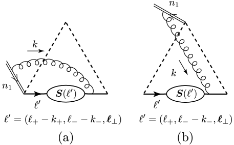
Figure 5: The diagrams that contribute to $\bm{S}_{(A_{2})}$ in Eq. (23).

The expression that corresponds to the diagrams that are shown in Fig. 5 is

$$\bm{S}_{(A_{2})}(\ell_{+},\ell_{-}) = ig_{s}^{2}C_{F}\left(\frac{\mu^{2}e^{\gamma_{E}}}{4\pi}\right)^{\epsilon}\int_{\bm{\ell}_{\perp}}\int\frac{dk_{+}dk_{-}d^{D-2}k_{\perp}}{(2\pi)^{D}}\frac{1}{(-k_{+}+i\varepsilon)(k^{2}+i\varepsilon)}$$ (29)

$$\times\Bigg{\{}-\frac{(\ell_{+}\frac{n\!\!\!/_{2}}{2}+\ell\!\!\!/_{\perp}+k\!\!\!/_{\perp}+m_{b})\frac{n\!\!\!/_{1}}{2}\bm{S}(\ell_{+}-k_{+},\ell_{-}-k_{-},\ell_{\perp})}{\ell_{+}\ell_{-}-(\bm{\ell}_{\perp}+\bm{k}_{\perp})^{2}-m_{b}^{2}+i\varepsilon}$$

$$\quad\quad+\frac{\left[(\ell_{+}+k_{+})\frac{n\!\!\!/_{2}}{2}+\ell\!\!\!/_{\perp}+k\!\!\!/_{\perp}+m_{b}\right]\frac{n\!\!\!/_{1}}{2}\bm{S}(\ell_{+},\ell_{-}-k_{-},\ell_{\perp})}{(\ell_{+}+k_{+})\ell_{-}-(\bm{\ell}_{\perp}+\bm{k}_{\perp})^{2}-m_{b}^{2}+i\varepsilon}\Bigg{\}}.$$

As we have done for diagrams $A_{1}$, we consider the case $\ell_{+}>0$, $\ell_{-}<0$. We wish to close the $k_{-}$ contour so as to avoid the singularities in the functions $\bm{S}$ on the right side of Eq. (29). Let us consider the first term in the curly brackets of Eq. (29). In complex $k_{-}$ plane, the pole of $\bm{S}(\ell_{+}-k_{+},\ell_{-}-k_{-},\ell_{\perp})$ exists in the upper half plane if $k_{+}<\ell_{+}$, and in the lower half plane if $k_{+}>\ell_{+}$. If $k_{+}<0$, all of the singularities are in the upper half plane, and the contour integration vanishes. Therefore, we need to consider the region $0<k_{+}<\ell_{+}$ and close the $k_{-}$ contour in the lower half plane to pick up the pole at $k_{-}=\frac{\bm{k}_{\perp}^{2}}{k_{+}}-i\varepsilon$:

$$\int\frac{dk_{+}dk_{-}d^{D-2}k_{\perp}}{(2\pi)^{D}}\frac{1}{-k_{+}+i\varepsilon}\frac{1}{k^{2}+i\varepsilon}\frac{(\ell_{+}\frac{n\!\!\!/_{2}}{2}+\ell\!\!\!/_{\perp}+k\!\!\!/_{\perp}+m_{b})\frac{n\!\!\!/_{1}}{2}\bm{S}(\ell_{+}-k_{+},\ell_{-}-k_{-},\ell_{\perp})}{\ell_{+}\ell_{-}-(\bm{\ell}_{\perp}+\bm{k}_{\perp})^{2}-m_{b}^{2}+i\varepsilon}$$ (30)

$$= 2\pi i\int\frac{d^{D-2}k_{\perp}}{(2\pi)^{D}}\int^{\ell_{+}}_{0}\frac{dk_{+}}{k_{+}^{2}}\frac{(\ell_{+}\frac{n\!\!\!/_{2}}{2}+\ell\!\!\!/_{\perp}+k\!\!\!/_{\perp}+m_{b})\frac{n\!\!\!/_{1}}{2}\bm{S}(\ell_{+}-k_{+},\ell_{-}-\frac{\bm{k}_{\perp}^{2}}{k_{+}},\ell_{\perp})}{\ell_{+}\ell_{-}-(\bm{\ell}_{\perp}+\bm{k}_{\perp})^{2}-m_{b}^{2}+i\varepsilon}.$$

Next let us consider the second term in the curly brackets of Eq. (29). The pole of $\bm{S}(\ell_{+},\ell_{-}-k_{-},\ell_{\perp})$ exists in the upper half plane when $\ell_{+}>0$. If $k_{+}<0$, all of the singularities are in the upper half plane, and the contour integration vanishes. Therefore, we need to consider the region $k_{+}>0$ and close the $k_{-}$ contour in the lower half plane to pick up the pole at $k_{-}=\frac{\bm{k}_{\perp}^{2}}{k_{+}}-i\varepsilon$:

$$\int\frac{dk_{+}dk_{-}d^{D-2}k_{\perp}}{(2\pi)^{D}}\frac{1}{-k_{+}+i\varepsilon}\frac{1}{k^{2}+i\varepsilon}\frac{((\ell_{+}+k_{+})\frac{n\!\!\!/_{2}}{2}+\ell\!\!\!/_{\perp}+k\!\!\!/_{\perp}+m_{b})\frac{n\!\!\!/_{1}}{2}\bm{S}(\ell_{+},\ell_{-}-k_{-},\ell_{\perp})}{(\ell_{+}+k_{+})\ell_{-}-(\bm{\ell}_{\perp}+\bm{k}_{\perp})^{2}-m_{b}^{2}+i\varepsilon}$$ (31)

$$= 2\pi i\int\frac{d^{D-2}k_{\perp}}{(2\pi)^{D}}\int_{0}^{\infty}\frac{dk_{+}}{k_{+}^{2}}\frac{((\ell_{+}+k_{+})\frac{n\!\!\!/_{2}}{2}+\ell\!\!\!/_{\perp}+k\!\!\!/_{\perp}+m_{b})\frac{n\!\!\!/_{1}}{2}\bm{S}(\ell_{+},\ell_{-}-\frac{\bm{k}_{\perp}^{2}}{k_{+}},\ell_{\perp})}{(\ell_{+}+k_{+})\ell_{-}-(\bm{\ell}_{\perp}+\bm{k}_{\perp})^{2}-m_{b}^{2}+i\varepsilon}.$$

Consequently, after the $k_{-}$ contour integrations, we can write Eq. (29) as follows:

$$\bm{S}_{(A_{2})}(\ell_{+},\ell_{-}) = 2\pi g_{s}^{2}C_{F}\left(\frac{\mu^{2}e^{\gamma_{E}}}{4\pi}\right)^{\epsilon}\int_{\bm{\ell}_{\perp}}\int\frac{d^{D-2}k_{\perp}}{(2\pi)^{D}}$$ (32)

$$\times\Bigg{\{}\int^{\ell_{+}}_{0}\frac{dk_{+}}{k_{+}^{2}}\frac{(\ell_{+}\frac{n\!\!\!/_{2}}{2}+\ell\!\!\!/_{\perp}+k\!\!\!/_{\perp}+m_{b})\frac{n\!\!\!/_{1}}{2}\bm{S}(\ell_{+}-k_{+},\ell_{-}-\frac{\bm{k}_{\perp}^{2}}{k_{+}},\ell_{\perp})}{\ell_{+}\ell_{-}-(\bm{\ell}_{\perp}+\bm{k}_{\perp})^{2}-m_{b}^{2}+i\varepsilon}$$

$$\quad~{}-\int_{0}^{\infty}\frac{dk_{+}}{k_{+}^{2}}\frac{((\ell_{+}+k_{+})\frac{n\!\!\!/_{2}}{2}+\ell\!\!\!/_{\perp}+k\!\!\!/_{\perp}+m_{b})\frac{n\!\!\!/_{1}}{2}\bm{S}(\ell_{+},\ell_{-}-\frac{\bm{k}_{\perp}^{2}}{k_{+}},\ell_{\perp})}{(\ell_{+}+k_{+})\ell_{-}-(\bm{\ell}_{\perp}+\bm{k}_{\perp})^{2}-m_{b}^{2}+i\varepsilon}\Bigg{\}}.\phantom{X}$$

UV divergences can potentially arise from the $\bm{k}_{\perp}$ or $k_{+}$ integrations in this expression. In order to test for one-loop UV divergences, we replace the all-orders soft function with the LO soft-quark propagator:

$$\bm{S}(\ell_{+}-k_{+},\ell_{-}-\tfrac{\bm{k}_{\perp}^{2}}{k_{+}},\ell_{\perp}) \to \frac{\frac{1}{2}(\ell_{+}-k_{+})\not{n}_{2}+\frac{1}{2}(\ell_{-}-\frac{\bm{k}_{\perp}^{2}}{\ell_{+}})\not{n}_{1}+\not{\ell}_{\perp}+m_{b}}{(\ell_{+}-k_{+})(\ell_{-}-\frac{\bm{k}_{\perp}^{2}}{\ell_{+}})-\bm{\ell}_{\perp}^{2}-m_{b}^{2}+i\varepsilon},$$

$$\bm{S}(\ell_{+},\ell_{-}-\tfrac{\bm{k}_{\perp}^{2}}{k_{+}},\ell_{\perp}) \to \frac{\frac{1}{2}\ell_{+}\not{n}_{2}+\frac{1}{2}(\ell_{-}-\frac{\bm{k}_{\perp}^{2}}{\ell_{+}})\not{n}_{1}+\not{\ell}_{\perp}+m_{b}}{\ell_{+}(\ell_{-}-\frac{\bm{k}_{\perp}^{2}}{\ell_{+}})-\bm{\ell}_{\perp}^{2}-m_{b}^{2}+i\varepsilon}.$$ (33)

Because of the numerator factors $\not{n}_{1}$ in Eq. (32), the terms in the propagator numerators that are proportional to $\not{n}_{1}$ vanish. It is then easy to see that the $\bm{k}_{\perp}$ and $k_{+}$ integrations are UV convergent. Therefore, the diagrams $A_{2}$ do not contribute to the one-loop renormalization of the soft function.

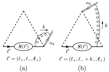
Figure 6: The diagrams that contribute to $\bm{S}_{(A_{3})}$ in Eq. (35).

The mirror images of the diagrams $A_{1}$, which we call $A_{3}$, are shown in Fig. 6. The expression that corresponds to these diagrams is

$$\bm{S}_{(A_{3})}(\ell_{+},\ell_{-},\ell_{\perp}) = ig_{s}^{2}C_{F}\left(\frac{\mu^{2}e^{\epsilon\gamma_{\textrm{E}}}}{4\pi}\right)^{\epsilon}\int_{\bm{\ell}_{\perp}}\int\frac{dk_{+}dk_{-}d^{D-2}k_{\perp}}{(2\pi)^{D}}\frac{1}{k_{-}+i\varepsilon}\frac{1}{k^{2}+i\varepsilon}$$ (34)

$$\times\Bigg{\{}\frac{\left[\frac{n\!\!\!/_{1}}{2}(\ell_{-}-k_{-})+\ell\!\!\!/_{\perp}-k\!\!\!/_{\perp}+m_{b}\right]\frac{n\!\!\!/_{2}}{2}\bm{S}(\ell_{+},\ell_{-},\ell_{\perp})}{(\ell_{+}-k_{+})(\ell_{-}-k_{-})-(\bm{\ell}_{\perp}-\bm{k}_{\perp})^{2}-m_{b}^{2}+i\varepsilon}$$

$$\quad\quad-\frac{(\frac{n\!\!\!/_{1}}{2}\ell_{-}+\ell\!\!\!/_{\perp}-k\!\!\!/_{\perp}+m_{b})\frac{n\!\!\!/_{2}}{2}\bm{S}(\ell_{+},\ell_{-}+k_{-},\ell_{\perp})}{(\ell_{+}-k_{+})\ell_{-}-(\bm{\ell}_{\perp}-\bm{k}_{\perp})^{2}-m_{b}^{2}+i\varepsilon}\Bigg{\}},$$

where the first term corresponds to the diagram in Fig. 6(a) and the second term corresponds to the diagram in Fig. 6(b). We treat this expression along the same lines as our treatment of the expression for the diagrams $A_{1}$, except that the roles of $k_{+}$ and $k_{-}$ are interchanged and, initially, we consider the case $\ell_{+}<0$, $\ell_{-}>0$. The result for the UV-divergent part, valid for all $\omega$, is

$$\bm{S}^{\text{UV}}_{(A_{3})}(\ell_{+},\ell_{-})$$ (35)

$$= \frac{\alpha_{s}C_{F}}{2\pi}\frac{1}{\epsilon_{\textrm{UV}}}\int_{\bm{\ell}_{\perp}}\Bigg{[}\left(1-\frac{n\!\!\!/_{2}n\!\!\!/_{1}}{4}+\frac{n_{1}\cdot\ell}{\omega}\frac{\ell\!\!\!/_{\perp}n\!\!\!/_{2}}{2}\right)\bm{S}(\ell_{+},\ell_{-},\ell_{\perp})$$

$$\quad\quad\quad\quad\quad\quad+\int_{0}^{\infty}dx\bigg{\{}\left[1-\frac{n\!\!\!/_{2}n\!\!\!/_{1}}{4}+\frac{n_{1}\cdot\ell}{(1+x)\omega}\frac{\ell\!\!\!/_{\perp}n\!\!\!/_{2}}{2}+\frac{m_{b}(n_{1}\cdot\ell)}{\omega}\frac{n\!\!\!/_{2}}{2}\right]\frac{\bm{S}(\ell_{+},(1+x)\ell_{-},\ell_{\perp})}{x(1+x)}$$

$$\quad\quad\quad\quad\quad\quad\quad\quad\quad\quad\quad-\left[1-\frac{n\!\!\!/_{2}n\!\!\!/_{1}}{4}+\frac{n_{1}\cdot\ell}{\omega}\frac{\ell\!\!\!/_{\perp}n\!\!\!/_{2}}{2}+\frac{m_{b}(n_{1}\cdot\ell)}{\omega}\frac{n\!\!\!/_{2}}{2}\right]\frac{\bm{S}(\ell_{+},\ell_{-},\ell_{\perp})}{x(1+x)}\bigg{\}}\Bigg{]}.$$

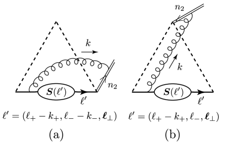
Figure 7: The diagrams that contribute to $\bm{S}_{(A_{4})}$ in Eq. (35).

The mirror images of the diagrams $A_{2}$, which we call $A_{4}$, are shown in Fig. 7. As with the case of diagrams $A_{2}$, the diagrams $A_{4}$ do not contribute the UV poles, and, so, do not contribute to the renormalization of the soft function.

X.2 Diagrams B

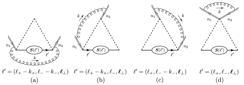
Figure 8: The diagrams that contribute to $\bm{S}_{(B)}$ in Eq. (36).

The expression that corresponds to the diagrams that are shown in Fig. 8 is

$$\bm{S}_{(B)}(\ell_{+},\ell_{-}) = ig_{s}^{2}C_{F}\left(\frac{\mu^{2}e^{\gamma_{\textrm{E}}}}{4\pi}\right)^{\epsilon}\int\frac{dk_{+}dk_{-}d^{D-2}k_{\perp}}{(2\pi)^{D}}\frac{1}{(-k_{+}+i\varepsilon)(k_{-}+i\varepsilon)(k^{2}+i\varepsilon)}$$ (36)

$$\times\left[\bm{S}(\ell_{+}-k_{+},\ell_{-}-k_{-})-\bm{S}(\ell_{+}-k_{+},\ell_{-})-\bm{S}(\ell_{+},\ell_{-}-k_{-})+\bm{S}(\ell_{+},\ell_{-})\right].\phantom{XX}$$

Here, we have carried out the integration over $\ell_{\perp}$, replacing the unintegrated soft functions on the right side of the equation with integrated soft functions.

For the expression in Eq. (36), we initially consider the case $\ell_{-}>0$, $\ell_{+}<0$. We choose to complete the $k_{-}$ integration first. We wish to close the $k_{-}$ contour so as to avoid the singularities in the functions $\bm{S}$ on the right side of Eq. (36). In the region $k_{+}>0$, all of the singularities are in the $k_{-}$ lower half-plane, and so the contour integration vanishes. Therefore, we need only consider the region $k_{+}<0$. For the first term in the brackets, we do the following: when $k_{+}<\ell_{+}$, we close the $k_{-}$ contour in the lower half-plane and pick up the pole at $k_{-}=-i\varepsilon$; when $\ell_{+}<k_{+}<0$, we close the $k_{-}$ contour in the upper half-plane and pick up the pole at $k_{-}=\frac{k_{\perp}^{2}}{k_{+}}+i\varepsilon$. For the second, third, and fourth terms in brackets in Eq. (36), we close the $k_{-}$ contour in the upper half-plane and pick up the pole at $k_{-}=\frac{k_{\perp}^{2}}{k_{+}}+i\varepsilon$. The results of the contour integrations are

$$\bm{S}_{(B)}(\ell_{+},\ell_{-}) = -2\alpha_{s}C_{F}\left(\frac{\mu^{2}e^{\gamma_{\textrm{E}}}}{4\pi}\right)^{\epsilon}\int_{-\infty}^{0}\frac{dk_{+}}{(-k_{+})}\int\frac{d^{D-2}k_{\perp}}{(2\pi)^{D-2}}\frac{1}{\bm{k}_{\perp}^{2}}$$ (37)

$$\times\bigg{[}\theta(\ell_{+}-k_{+})\bm{S}(\ell_{+}-k_{+},\ell_{-})+\theta(k_{+}-\ell_{+})\bm{S}(\ell_{+}-k_{+},\ell_{-}-\tfrac{\bm{k}_{\perp}^{2}}{k_{+}})$$

$$\quad-\bm{S}(\ell_{+}-k_{+},\ell_{-})-\bm{S}(\ell_{+},\ell_{-}-\tfrac{\bm{k}_{\perp}^{2}}{k_{+}})+\bm{S}(\ell_{+},\ell_{-})\bigg{]}.$$

It is apparent that the rapidity divergences that appear as $k_{+}\to 0$ and as $k_{+}\to-\infty$ with $\bm{k}_{\perp}^{2}$ fixed cancel in Eq. (37). This is as expected, since the upper semi-infinite Wilson lines cancel against the lower semi-infinite Wilson lines to produce finite-length Wilson lines. We note that the IR divergences that appear as $\bm{k}_{\perp}^{2}\rightarrow 0$ also cancel, reflecting the fact that the soft function is IR finite.

Making the change of variables $\bm{k}_{\perp}^{2}=xk_{+}\ell_{-}$ and splitting the $k_{+}$ integration region $[-\infty,0]$ into $[-\infty,\ell_{+}]$ and $[\ell_{+},0]$, we obtain

$$\bm{S}_{(B)}(\ell_{+},\ell_{-}) = \frac{\alpha_{s}C_{F}}{2\pi}\frac{\left(\mu^{2}e^{\gamma_{\textrm{E}}}\right)^{\epsilon}}{\Gamma(1-\epsilon)}(\ell_{-})^{-\epsilon}\int_{-\infty}^{0}dx\frac{1}{(-x)^{1+\epsilon}}$$ (38)

$$\times\bigg{\{}\int_{\ell_{+}}^{0}\frac{dk_{+}}{(-k_{+})^{1+\epsilon}}\Big{[}\bm{S}(\ell_{+}-k_{+},\ell_{-})-\bm{S}(\ell_{+}-k_{+},\ell_{-}(1-x))$$

$$\quad\quad\quad\quad\quad\quad\quad\quad+\bm{S}(\ell_{+},\ell_{-}(1-x))-\bm{S}(\ell_{+},\ell_{-})\Big{]}$$

$$\quad+\int_{-\infty}^{\ell_{+}}\frac{dk_{+}}{(-k_{+})^{1+\epsilon}}\Big{[}\bm{S}(\ell_{+},\ell_{-}(1-x))-\bm{S}(\ell_{+},\ell_{-})\Big{]}\bigg{\}}.$$

In Eq. (38), there are no divergences as $k_{+}\to 0$ or as $\bm{k}_{\perp}^{2}\to 0$. All of the UV poles come either from the region $x\to-\infty$ and/or the region $k_{+}\to-\infty$. We test for one-loop UV divergences by replacing the all-orders soft functions with LO soft-quark propagators. Then, we see that the $x\to-\infty$ region gives a UV pole only if the argument of $\bm{S}$ is independent of $x$ and that the $k_{+}\to-\infty$ region gives a UV pole only if the argument of $\bm{S}$ is independent of $k_{+}$. It follows that the second and third terms in the integrand of the $k_{+}$ integration with the range $[\ell_{+},0]$ do not contribute UV poles. We extract the UV-pole contributions from the other terms. Then, for the remaining finite integration over $k_{+}$, we make the variable change $k_{+}=x\ell_{+}$. The result is

$$\bm{S}_{(B)}^{\textrm{UV}}(\ell_{+},\ell_{-})$$ (39)

$$= \frac{\alpha_{s}C_{F}}{2\pi}\frac{1}{\epsilon_{\textrm{UV}}}\Bigg{\{}-\left[\frac{1}{\epsilon_{\textrm{UV}}}+\log\left(\frac{\mu^{2}}{-\omega-i\varepsilon}\right)\right]\bm{S}(\ell_{+},\ell_{-})-\int_{-1}^{0}dx\frac{\bm{S}(\ell_{+},\ell_{-}(1-x))-\bm{S}(\ell_{+},\ell_{-})}{x}$$

$$\quad\quad\quad\quad\quad+\int_{0}^{1}dx\frac{\bm{S}(\ell_{+}(1-x),\ell_{-})-\bm{S}(\ell_{+},\ell_{-})}{x}-\int_{-\infty}^{-1}dx\frac{\bm{S}(\ell_{+},\ell_{-}(1-x))}{x}\Bigg{\}}.$$

Here, we have inserted a term $-i\varepsilon$ into the argument of the logarithm. This prescription is not necessary for the current case $\omega=\ell_{+}\ell_{-}<0$. However, with this change, we can see that Eq. (39) actually gives the correct analytic continuation of the function on the right side for all $\omega$ in the complex plane. Because the factors $(1-x)$ in the arguments of $\bm{S}$ are non-negative over all of the ranges of integration, the right side of Eq. (39) has the property that it is analytic for all $\omega$, except for a cut along positive real axis that lies just below the axis, which is the correct analyticity structure for the soft function on the left side of Eq. (39).

In the application of the soft function to the process $H\to\gamma\gamma$ through a $b$-quark loop, one integrates the soft function over $\ell_{\perp}$ and takes the discontinuity. The analytic continuation in Eq. (39) is not suited for this purpose because, if one carries out the integration over $\ell_{\perp}$ and takes the discontinuity inside the infinite-range $x$ integration, the resulting $x$ integration is divergent. This is easily seen from the LO expression for $\bm{S}$ in Eq. (19).

In order to remedy this situation, we rewrite the expression in Eq. (39). First, we write the integrations over negative values of $x$ as

$$-\int_{-\infty}^{-1}\frac{dx}{x}{\bm{S}}(\ell_{+},\ell_{-}(1-x))-\int_{-1}^{0}\frac{dx}{x}~{}\left[\bm{S}(\ell_{+},\ell_{-}(1-x))-\bm{S}(\ell_{+},\ell_{-})\right]$$ (40)

$$= \lim_{\delta\to 0}\left[-\int_{-\infty}^{-\delta}\frac{dx}{x}\bm{S}(\ell_{+},\ell_{-}(1-x))-\int_{-1}^{-\delta}\frac{dx}{x}\bm{S}(\ell_{+},\ell_{-})\right].$$

We consider the first term in brackets on the right side of Eq. (40). There are two cases: (i) when $0\leq\mathrm{arg}(\omega)<\pi$, $\bm{S}(\ell_{+},\ell_{-}(1-x))$ has a cut that extends from $x=1$ into the $x$ lower half-plane and is otherwise analytic, (ii) when $-\pi<\mathrm{arg}(\omega)<0$, $\bm{S}(\ell_{+},\ell_{-}(1-x))$ has a cut that extends from $x=1$ into the $x$ upper half-plane and is otherwise analytic. For case (i) [(ii)], we deform the $x$ contour of integration into the upper [lower] half-plane into a semicircle at infinity, a line from $\infty$ to $\delta$, and a small semicircle from $\delta$ to $-\delta$ that is traversed in the counterclockwise [clockwise] direction. The contribution of the semicircle at infinity vanishes, and the contribution of the small semicircle is $\pm i\pi S(\omega)$, where the upper [lower] sign corresponds to case (i) [(ii)]. For the second term in brackets on the right side of Eq. (40), we make the change of variables $x\to-x$. With these transformations, the expression in Eq. (39) becomes

$$\bm{S}_{(B)}^{\textrm{UV}}(\ell_{+},\ell_{-}) = \frac{\alpha_{s}C_{F}}{2\pi}\frac{1}{\epsilon_{\textrm{UV}}}\Bigg{\{}-\left[\frac{1}{\epsilon_{\textrm{UV}}}+\log\left(\frac{\mu^{2}}{\omega+i\varepsilon}\right)\right]\bm{S}(\ell_{+},\ell_{-})+\int_{1}^{\infty}dx\frac{\bm{S}(\ell_{+},\ell_{-}(1-x))}{x}$$ (41)

$$\quad\quad\quad\quad\quad+\int_{0}^{1}dx\frac{\bm{S}(\ell_{+}(1-x),\ell_{-})+\bm{S}(\ell_{+},\ell_{-}(1-x))-2\bm{S}(\ell_{+},\ell_{-})}{x}\Bigg{\}}.\phantom{XX}$$

This expression is also a valid analytic continuation of $\bm{S}_{(B)}^{\textrm{UV}}$ for all $\omega$, and it is suitable for use in the application $H\to\gamma\gamma$ through a $b$-quark loop.

X.3 Quark self-energy diagram

There is also a contribution to the one-loop UV divergences that arises from the one-loop quark self-energy diagram. As we have already remarked, the UV divergence that is associated with the quark-mass renormalization is removed by the standard QCD counterterm, and only the wave-function-renormalization divergence contributes to the soft-operator renormalization. It is given by

$$\bm{S}_{(C)}^{\text{UV}}(\ell_{+},\ell_{-}) = -\frac{\alpha_{s}C_{F}}{4\pi}\frac{1}{\epsilon_{\text{UV}}}\bm{S}(\ell_{+},\ell_{-}).$$ (42)

X.4 $\textbf{{Z}}_{\!\textbf{{S}}}$ at one-loop order

Now let us summarize the one-loop contributions to the UV poles of the integrated soft function $\bm{S}(\ell_{+},\ell_{-})$ for the case $\ell_{+}>0$, $\ell_{-}>0$:

$$\bm{S}^{\textrm{UV}}(\ell_{+},\ell_{-})$$ (43)

$$= \bm{S}^{\textrm{UV}}_{(A_{1})}(\ell_{+},\ell_{-})+\bm{S}^{\textrm{UV}}_{(A_{3})}(\ell_{+},\ell_{-})+\bm{S}^{\textrm{UV}}_{(B)}(\ell_{+},\ell_{-})+\bm{S}^{\textrm{UV}}_{(C)}(\ell_{+},\ell_{-})$$

$$= \frac{\alpha_{s}C_{F}}{2\pi}\frac{1}{\epsilon_{\textrm{UV}}}\int_{\bm{\ell}_{\perp}}\Bigg{[}\bm{S}(\ell_{+},\ell_{-},\ell_{\perp})\left(1-\frac{n\!\!\!/_{2}n\!\!\!/_{1}}{4}+\frac{n_{2}\cdot\ell}{\omega}\frac{n\!\!\!/_{1}\ell\!\!\!/_{\perp}}{2}\right)$$

$$\quad\quad\quad\quad\quad\quad+\int_{0}^{\infty}dx\bigg{\{}\frac{\bm{S}(\ell_{+}(1+x),\ell_{-},\ell_{\perp})}{x(1+x)}\left[1-\frac{n\!\!\!/_{2}n\!\!\!/_{1}}{4}+\frac{n_{2}\cdot\ell}{(1+x)\omega}\frac{n\!\!\!/_{1}\ell\!\!\!/_{\perp}}{2}+\frac{m_{b}(n_{2}\cdot\ell)}{\omega}\frac{n\!\!\!/_{1}}{2}\right]$$

$$\quad\quad\quad\quad\quad\quad\quad\quad\quad\quad\quad-\frac{\bm{S}(\ell_{+},\ell_{-},\ell_{\perp})}{x(1+x)}\left[1-\frac{n\!\!\!/_{2}n\!\!\!/_{1}}{4}+\frac{n_{2}\cdot\ell}{\omega}\frac{n\!\!\!/_{1}\ell\!\!\!/_{\perp}}{2}+\frac{m_{b}(n_{2}\cdot\ell)}{\omega}\frac{n\!\!\!/_{1}}{2}\right]\bigg{\}}\Bigg{]}$$

$$+\frac{\alpha_{s}C_{F}}{2\pi}\frac{1}{\epsilon_{\textrm{UV}}}\int_{\bm{\ell}_{\perp}}\Bigg{[}\left(1-\frac{n\!\!\!/_{2}n\!\!\!/_{1}}{4}+\frac{n_{1}\cdot\ell}{\omega}\frac{\ell\!\!\!/_{\perp}n\!\!\!/_{2}}{2}\right)\bm{S}(\ell_{+},\ell_{-},\ell_{\perp})$$

$$\quad\quad\quad\quad\quad\quad+\int_{0}^{\infty}dx\bigg{\{}\left[1-\frac{n\!\!\!/_{2}n\!\!\!/_{1}}{4}+\frac{n_{1}\cdot\ell}{(1+x)\omega}\frac{\ell\!\!\!/_{\perp}n\!\!\!/_{2}}{2}+\frac{m_{b}(n_{1}\cdot\ell)}{\omega}\frac{n\!\!\!/_{2}}{2}\right]\frac{\bm{S}(\ell_{+},(1+x)\ell_{-},\ell_{\perp})}{x(1+x)}$$

$$\quad\quad\quad\quad\quad\quad\quad\quad\quad\quad-\left[1-\frac{n\!\!\!/_{2}n\!\!\!/_{1}}{4}+\frac{n_{1}\cdot\ell}{\omega}\frac{\ell\!\!\!/_{\perp}n\!\!\!/_{2}}{2}+\frac{m_{b}(n_{1}\cdot\ell)}{\omega}\frac{n\!\!\!/_{2}}{2}\right]\frac{\bm{S}(\ell_{+},\ell_{-},\ell_{\perp})}{x(1+x)}\bigg{\}}\Bigg{]}$$

$$+\frac{\alpha_{s}C_{F}}{2\pi}\frac{1}{\epsilon_{\textrm{UV}}}\Bigg{\{}-\left[\frac{1}{\epsilon_{\textrm{UV}}}+\log\left(\frac{\mu^{2}}{\omega}\right)\right]\bm{S}(\ell_{+},\ell_{-})+\int_{1}^{\infty}dx\frac{\bm{S}(\ell_{+},\ell_{-}(1-x))}{x}$$

$$\quad\quad\quad\quad\quad+\int_{0}^{1}dx\frac{\bm{S}(\ell_{+}(1-x),\ell_{-})+\bm{S}(\ell_{+},\ell_{-}(1-x))-2\bm{S}(\ell_{+},\ell_{-})}{x}\Bigg{\}}$$

$$-\frac{\alpha_{s}C_{F}}{4\pi}\frac{1}{\epsilon_{\textrm{UV}}}\int_{\bm{\ell}_{\perp}}\bm{S}(\ell_{+},\ell_{-},\ell_{\perp}).$$

We note that this expression contains contributions in which the argument of $\bm{S}$ is shifted away from $(\ell_{+},\ell_{-},\ell_{\perp})$. As we have seen, these nonlocal contributions arise because of unorthodox momentum routing in the soft function that is required to factor the soft function from the jet functions.

Since, $\bm{S}(\ell_{+},\ell_{-})$ has no singularities on the real $\omega=\ell_{+}\ell_{-}$ axis for $\omega<0$, the contribution in Eq. (43) that is proportional to $\int_{1}^{\infty}dx\bm{S}(\ell_{+},\ell_{-}(1-x))/x$ gives a vanishing contribution to the discontinuity of $\bm{S}^{\rm UV}(\ell_{+},\ell_{-})$. Therefore, we drop this contribution in subsequent discussions.

We can express the discontinuity of the renormalized soft function $S^{\text{R}}(\ell_{+},\ell_{-})$ in terms of the discontinuities of its structure functions. We wish to renormalize the structure functions that are given in Eq. (15). However, the $\ell_{\perp}$-dependent terms in Eq. (43) mix additional structure functions into the structure functions in Eq. (15). These additional structure functions are

$$\bm{S}_{i}(\omega)=\displaystyle\int_{\bm{\ell}_{\perp}}\bm{S}_{i}(\omega,\bm{\ell}_{\perp}^{2})\frac{\bm{\ell}_{\perp}^{2}}{\omega},\quad\textrm{for $i=5$, $6$, $7$, and $8$}.$$ (44)

We note that the renormalizations of these additional structure functions involve new structure functions, and so on, ad infinitum. We do not write out the renormalizations of these additional structure functions.

Using Eq. (43) as a starting point, we can write the renormalized forms of the discontinuities of the structure functions $S_{1}^{R}$–$S_{4}^{R}$ as convolution integrals. We make the following changes of integration variables: $\omega^{\prime}=(1+x)\omega$ for $\bm{S}_{(A_{1})}^{\rm UV}$ and $\bm{S}_{(A_{3})}^{\rm UV}$, and $\omega^{\prime}=(1-x)\omega$ for $\bm{S}_{(B)}^{\rm UV}$. The result is

$$S_{i}^{\textrm{R}}(\omega)=\sum_{j=1}^{8}\int_{0}^{\infty}d\omega^{\prime}Z_{S}^{ij}(\omega,\omega^{\prime};\mu)S_{j}(\omega^{\prime}),\quad\textrm{for $i=$1, 2, 3, and 4,}$$ (45)

where

$$Z_{S}^{ij}(\omega,\omega^{\prime};\mu)=\delta(\omega-\omega^{\prime})\delta^{ij}+\frac{\alpha_{s}C_{F}}{4\pi}\frac{1}{\epsilon_{\textrm{UV}}}\bm{M}_{S}^{ij}(\omega,\omega^{\prime};\mu),$$ (46)

and the matrix representation of $\bm{M}_{S}^{ij}(\omega,\omega^{\prime};\mu)$ is given by

$$\bm{M}_{S}(\omega,\omega^{\prime};\mu)$$

$$\!\!\!\!\!\!\!\!\!=\begin{pmatrix}d-2a-2b-2c&0&0&0&0&0&0&0\\ -\frac{m_{b}^{2}}{\omega}b&d-a-\frac{\omega^{\prime}}{\omega}b-\frac{\omega^{\prime}+\omega}{\omega}c&0&0&-(a+b)&0&0&0\\ -\frac{m_{b}^{2}}{\omega}b&0&d-a-\frac{\omega^{\prime}}{\omega}b-\frac{\omega^{\prime}+\omega}{\omega}c&0&-(a+b)&0&0&0\\ 2(a+b)&-\frac{\omega^{\prime}}{\omega}b&-\frac{\omega^{\prime}}{\omega}b&d-2c&0&a+b&a+b&0\end{pmatrix},$$

with $a$, $b$, $c$, and $d$ defined by

$$a = 2\delta(\omega-\omega^{\prime}),$$

$$b = 2\left[\frac{\omega\theta(\omega^{\prime}-\omega)}{\omega^{\prime}(\omega^{\prime}-\omega)}\right]_{+},$$

$$c = 2\left[\frac{\theta(\omega-\omega^{\prime})}{\omega-\omega^{\prime}}\right]_{+},$$

$$d = \left[\frac{2}{\epsilon_{\textrm{UV}}}+2\log\left(\frac{\mu^{2}}{\omega}\right)+1\right]\delta(\omega-\omega^{\prime}).$$ (48)

Here, the plus distribution is defined by

$$\int_{0}^{\infty}d\omega^{\prime}\frac{f(\omega^{\prime})}{[g(\omega^{\prime})]_{+}}=\int_{0}^{\infty}d\omega^{\prime}\frac{f(\omega^{\prime})-f(\omega)}{g(\omega^{\prime})}.$$ (49)

The plus distributions correspond to the nonlocal contributions in Eq. (43), while the $\delta$ function corresponds to the local contributions.

In Eq. (45), we have written down the renormalization of the soft function for a general Dirac structure. Only the structure function $S_{1}$ is relevant for the process $H\rightarrow\gamma\gamma$ through a $b$-quark loop because the radiative jet functions in $\langle\gamma\gamma|{\cal O}_{3}|H\rangle$ produce a factor $\not{n}_{2}$ on the left of the soft function and a factor $\not{n}_{1}$ on the right of the soft function, which project out the structure function ${S}_{1}$. However, we have included the other Dirac structures in Eq. (45) because of the possibility that they might be relevant for exclusive processes other than $H\rightarrow\gamma\gamma$ through a $b$-quark loop.

Because the matrix in Eq. (X.4) mixes ${S}_{5}$–${S}_{8}$ with ${S}_{1}$–${S}_{4}$, it is not possible to write a closed-form evolution equation for all of ${S}_{1}$–${S}_{4}$. Therefore, we specialize to the case of ${S}_{1}$, for which there is no mixing in the renormalization. For ${S}_{1}$, we have

$$Z_{S}^{11} = \delta(\omega^{\prime}-\omega)+\frac{\alpha_{s}C_{F}}{4\pi}\frac{1}{\epsilon_{\text{UV}}}\left(d-2a-2b-2c\right)$$ (50)

$$= \delta(\omega^{\prime}-\omega)+\frac{\alpha_{s}C_{F}}{4\pi}\frac{1}{\epsilon_{\text{UV}}}\bigg{\{}\left[\frac{2}{\epsilon_{\text{UV}}}+2\log\left(\frac{\mu^{2}}{\omega}\right)-3\right]\delta(\omega^{\prime}-\omega)$$

$$\quad\quad\quad\quad\quad\quad\quad\quad\quad\quad-4\omega\left[\frac{\theta(\omega^{\prime}-\omega)}{\omega^{\prime}(\omega^{\prime}-\omega)}+\frac{\theta(\omega-\omega^{\prime})}{\omega(\omega-\omega^{\prime})}\right]_{+}\bigg{\}}.$$

This result confirms the conjecture in Ref. Liu:2020eqe for the renormalization of the soft function in order $\alpha_{s}$. It is consistent with the explicit calculation of the soft function in order $\alpha_{s}$ that is given in Eqs. (4.7)–(4.8) of Ref. Liu:2019oav . Note, however, that one cannot deduce the form of the one-loop renormalization and evolution of the soft function from the order-$\alpha_{s}$ contribution to the soft function because, once the integration over $\omega^{\prime}$ in Eq. (45), has been carried out, the nonlocal renormalization factor $Z_{S}$ cannot be reconstructed.

X.5 One-loop evolution equation

We obtain the evolution equation for $S_{1}$ by differentiating Eq. (45) with respect to the renormalization scale $\mu$:

$$\frac{d}{d\log{\mu}}S_{1}^{\textrm{R}}(\omega,\mu)=-\int_{0}^{\infty}d\omega^{\prime}\,\gamma_{S}(\omega,\omega^{\prime},\mu)S_{1}^{\textrm{R}}(\omega^{\prime},\mu),$$ (51)

where

$$\gamma_{S}(\omega,\omega^{\prime},\mu) = -\frac{d\log{Z_{S}^{11}}}{d\log{\mu}}$$ (52)

$$= -\frac{\alpha_{s}C_{F}}{4\pi}\Bigg{\{}\left[4\log{\left(\frac{\omega}{\mu^{2}}\right)}+6\right]\delta\left(\omega^{\prime}-\omega\right)$$

$$\quad\quad\quad\quad+8\omega\left[\frac{\theta(\omega^{\prime}-\omega)}{\omega^{\prime}(\omega^{\prime}-\omega)}+\frac{\theta(\omega-\omega^{\prime})}{\omega(\omega-\omega^{\prime})}\right]_{+}\Bigg{\}}+\mathcal{O}\left(\alpha_{s}^{2}\right),$$

and we have made use of the order-$\alpha_{s}$ dependence of $\alpha_{s}$ on $\mu$, which is given by

$$\frac{d\alpha_{s}}{d\log{\mu}}=-2\epsilon\alpha_{s}+\mathcal{O}\left(\alpha_{s}^{2}\right).$$ (53)

This result confirms the conjecture in Ref. Liu:2020eqe for the one-loop evolution of the soft function.

XI Summary

In this paper we have presented a method for computing the renormalization and evolution of the soft function that appears in the factorization theorem for Higgs-boson decay to two photons through a $b$-quark loop Liu:2019oav . The renormalization is not straightforward because the factorization of the soft function from the jet functions leads to an unorthodox routing of loop momenta in the soft function. That unorthodox momentum routing results in nonlocal contributions to the renormalization and evolution of the soft function.

Our analysis of the renormalization of the soft function makes use of its analyticity properties. In Ref. Liu:2019oav , it was asserted that the soft function is analytic in the $\omega$ complex plane, except for singularities on the nonnegative real axis. ($\omega$ is the product of the longitudinal momenta that are carried by the soft function.) Somewhat surprisingly, the singularities extend to values of $\omega$ that are less than $m_{b}^{2}$. We have shown, through explicit examples in light-front perturbation theory, that such singularities arise because a $b$-quark line can carry an infinite longitudinal loop momentum, resulting in the vanishing of the $b$-quark intermediate-state light-front energy. We have also argued, making use of light-front perturbation theory, that the soft function is analytic everywhere in the complex $\omega$ plane, except for the nonnegative real axis, thus confirming the assertion in Ref. Liu:2019oav .

We have given an explicit calculation of the one-loop renormalization and evolution of the soft function. Our result for the one-loop renormalization is consistent with the calculation of the order-$\alpha_{s}$ contribution to the soft function in Ref. Liu:2019oav . Note, however, that one cannot deduce the nonlocal form of the one-loop renormalization/evolution of the soft function from the order-$\alpha_{s}$ contribution to the soft function because the renormalization/evolution involves a convolution with respect to $\omega$ of the nonlocal renormalization factor $Z_{S}$ with the soft function. One must make the convolution explicit in order to deduce $Z_{S}$.

Our results for the one-loop renormalization and evolution of the soft function confirm the conjectured one-loop form in Ref. Liu:2020eqe . This puts on a solid footing the one-loop contribution to the evolution kernel for the soft function, which is used to resum logarithms of $m_{H}^{2}/m_{b}^{2}$. The two-loop contribution to evolution kernel would be required to achieve greater precision in the resummation of logarithms of $m_{H}^{2}/m_{b}^{2}$. The form of the two-loop renormalization renormalization of the soft function has also been conjectured in Ref. Liu:2020eqe , and it is important to check that conjecture through explicit calculations. In principle, the methods that we have presented generalize straightforwardly to higher-order calculations of the renormalization and evolution of the soft function. However, because it is necessary to single out the longitudinal components of the loop momenta in order to capture the nonlocal nature of the renormalizations, one cannot use standard two-loop methods in such calculations, and the calculations may be technically challenging.

The unorthodox momentum routing in the soft function that we have noted in this paper arises because the soft function contains a soft-quark line, in contrast with the purely gluonic soft functions that arise in typical leading-power factorization theorems. The soft-quark line appears because the physical process first occurs at subleading power in the quark mass ($m_{b}^{1}$). At subleading power in the quark mass, a soft-quark pinch singularity can give a relative order-one contribution Bodwin:2014dqa . Hence, we expect this phenomenon to appear in any exclusive process that proceeds through a quark helicity flip, and the methods that we have presented in this paper should be applicable in those situations. For example, those methods may be relevant to the renormalization of soft function in the, as yet unproven, factorization theorem for the amplitude for $e^{+}e^{-}\to J/\psi+\eta_{c}$.

Appendix A Analyticity of the soft function: examples

In this appendix, we present some one-loop examples to illustrate the analyticity properties of the soft function. We consider all of the one-loop contributions to the soft function. We find that some of the diagrams contain denominators that can vanish for all $\omega\geq 0$, and, hence, contribute to an imaginary part. We also find, as expected from our general argument in Sec. VIII, that none of the denominators can vanish if $\omega$ is negative.

Our arguments rely on the use of light-front perturbation theory, whose Feynman rules we now summarize. In light-front perturbation theory, expressions for Feynman diagrams consist of (i) vertices, whose Feynman rules are the same as in covariant perturbation theory, (ii) energy denominators for each intermediate state, which consist of the incoming light-front energy minus the on-shell light-front energies of the particles that are included in the intermediate state, (iii) factors of the inverse of the longitudinal ($+$) momenta of the intermediate-state particles, and (iv) integrations over the $+$ and transverse components of the loop momenta Collins:2011zzd ; Chang:1968bh ; Kogut:1969xa ; Yan:1973qg . The vertices are assigned an ordering in $x_{+}$. For each intermediate-state line, the allowed propagation is from lower to higher $x_{+}$, and, so the longitudinal component of momentum is positive. We have drawn the figures in this appendix to indicate the light-front time orderings. We note that the points $X$ and $Z$ are at equal light-front time.

In our case, there are also Wilson lines present. The $n_{1}$ Wilson line is instantaneous in light-front time. That is, it does not propagate. Therefore, it simply produces an overall factor. In the case of the $n_{2}$ Wilson line, the open end is always at light-front time $-\infty$ and the vertex end is at some finite light-front time. It has intermediate-state energy zero.

The analyticity of the soft function is described by the analyticity of its structure functions. As we have seen, the structure functions are functions of the product $\ell_{+}\ell_{-}$. Therefore, in considering the analyticity of the structure functions as a function of $\omega=\ell_{+}\ell_{-}$, we can, without loss of generality, take $\ell_{+}>0$.

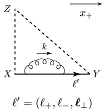
Figure 9: Quark self-energy diagram.

Let us begin by considering the quark self-energy diagram in Fig. 9. The corresponding propagator denominators in covariant perturbation theory are given by

$$\frac{1}{k_{+}k_{-}-\bm{k}_{\perp}^{2}+i\varepsilon}\frac{1}{(\ell_{+}-k_{+})(\ell_{-}-k_{-})-(\bm{\ell}_{\perp}-\bm{k}_{\perp})^{2}-m_{b}^{2}+i\varepsilon}.$$ (54)

The $k_{-}$ contour integration gives a nonzero result only if $0<k_{+}<\ell_{+}$. We close the $k_{-}$ contour of integration in the lower half-plane, picking up the gluon pole at $k_{-}=\bm{k}_{\perp}^{2}/k_{+}-i\varepsilon$, to obtain a result that is proportional to

$$-2\pi i\theta(k_{+})\theta(\ell_{+}-k_{+})\frac{1}{k_{+}}\frac{1}{\ell_{+}-k_{+}}\frac{1}{\ell_{-}-\bm{k}_{\perp}^{2}/k_{+}-[(\bm{\ell}_{\perp}-\bm{k}_{\perp})^{2}+m_{b}^{2}]/(\ell_{+}-k_{+})+i\varepsilon}.$$ (55)

This expression has a simple interpretation in light-front perturbation theory. The $\theta$ functions enforce the positivity of the $+$ light-front longitudinal momenta. The next two factors are the light-front normalizations of the gluon and soft-quark propagators, respectively. The denominator in the last factor is the light-front energy denominator from the intermediate state that consists of the gluon and the soft-quark. In the energy denominator, $\ell_{-}$ is the light-front energy, $\bm{k}_{\perp}^{2}/k_{+}$ is the gluon intermediate-state energy, and $[(\bm{\ell}_{\perp}-\bm{k}_{\perp})^{2}+m_{b}^{2}]/(\ell_{+}-k_{+})$ is the soft-quark intermediate-state energy. We see that, owing to the constraints that are imposed by the positivity of the $+$ light-front longitudinal momenta, $k_{+}$ is always finite. Consequently, the energy denominator cannot vanish, and thereby produce an imaginary part, unless $\omega=\ell_{+}\ell_{-}\geq m_{b}^{2}$.

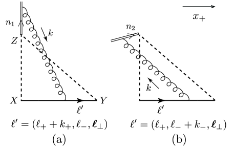
Figure 10: Diagrams that illustrate the analyticity properties of the soft function, as is explained in the text.

Next, we consider the diagram of Fig. 10(a). The corresponding propagator denominators in covariant perturbation theory are given by

$$\frac{1}{-k_{+}+i\varepsilon}\frac{1}{k^{2}+i\varepsilon}\frac{1}{(\ell_{+}+k_{+})\ell_{-}-\bm{\ell}_{\perp}^{2}-m_{b}^{2}+i\varepsilon}\frac{1}{\ell_{+}(\ell_{-}-k_{-})-(\bm{\ell}_{\perp}-\bm{k}_{\perp})^{2}-m_{b}^{2}+i\varepsilon}.\phantom{X}$$ (56)

For $\ell_{+}>0$, all of the poles in the $k_{-}$ complex plane are in the upper half-plane unless $k_{+}>0$. Hence, we close the $k_{-}$ contour of integration in the lower half-plane, picking up the residue of the pole from the gluon propagator at $k_{-}=\bm{k}_{\perp}^{2}/k_{+}-i\varepsilon$ to obtain a result that is proportional to

$$-2\pi i\theta(k_{+})\frac{1}{\ell_{+}}\frac{1}{\ell_{+}+k_{+}}\frac{1}{k_{+}}\frac{1}{-k_{+}+i\varepsilon}\frac{1}{\ell_{-}-\bm{k}_{\perp}^{2}/k_{+}-[(\bm{\ell}_{\perp}-\bm{k}_{\perp})^{2}+m_{b}^{2}]/\ell_{+}+i\varepsilon}$$

$$\times\frac{1}{\ell_{-}-(\bm{\ell}_{\perp}^{2}+m_{b}^{2})/(\ell_{+}+k_{+})+i\varepsilon}.$$ (57)

This expression also has a simple interpretation in light-front perturbation theory: the $\theta$ function enforces the forward propagation of the gluon; the next three factors are the light-front normalizations of the left-hand and right-hand soft-quark propagators and the gluon, respectively; the next factor comes from the instantaneous Wilson-line propagator; the next factor is the energy denominator from the intermediate state that consists of the gluon and the left-hand soft-quark propagator; the last factor is the light-front energy denominator from the intermediate state that consists of the right-hand soft-quark line. We see that in this case, in contrast with the case of the quark self-energy diagram, the momentum $k_{+}$ can become infinite without resulting in a negative longitudinal momentum in any of the particle lines. This is a consequence of the unorthodox routing of the momentum $k_{+}$, which appears in the right-hand soft-quark propagator, rather than in the left-hand soft-quark propagator. Then, for sufficiently large $k_{+}$, the second energy denominator can vanish for $\ell_{-}\geq 0$, producing and imaginary part. Note that the energy denominator can never vanish for $\ell_{-}<0$ because all of the intermediate-state energies are positive.

In the remaining examples in this Appendix, we couch the discussion in terms of light-front perturbation theory. However, it should be remembered that one can obtain the light-front expressions that appear in the discussions by integrating the covariant-perturbation-theory expressions over $k_{-}$, as we have done in the examples above.

A light-front analysis of the denominators of the diagram of Fig.10(b) yields

$$-2\pi i\theta(-k_{+})\frac{1}{\ell_{+}}\frac{1}{k_{+}}\frac{1}{\ell_{+}-k_{+}}\frac{1}{\bm{k}_{\perp}^{2}/k_{+}}\frac{1}{\ell_{-}+\bm{k}_{\perp}^{2}/k_{+}-(\bm{\ell}_{\perp}^{2}+m_{b}^{2})/\ell_{+}+i\varepsilon}$$

$$\times\frac{1}{\ell_{-}-[(\bm{\ell}_{\perp}-\bm{k}_{\perp})^{2}+m_{b}^{2}]/(\ell_{+}-k_{+})+i\varepsilon}.$$ (58)

Here, the denominator $\bm{k}_{\perp}^{2}/k_{+}$ is the energy denominator from the left-most intermediate state, which consists of the gluon and Wilson line. Because this intermediate state appears at an earlier light-front time than the injection of the light-front energy $\ell_{-}$, it has vanishing initial light-front energy. We note also that the on-shell Wilson line in the intermediate state has light-front energy zero. Because of the unorthodox momentum routing, $-k_{+}$ can reach positive infinity without causing of any of the particle lines to move backward. Consequently, for $-k_{+}$ sufficiently large, the intermediate state in the third energy denominator can have zero light-front energy, and it produces an imaginary part for $\ell_{-}\geq 0$. Since all of the intermediate-state light-front energies are positive, neither energy denominator can vanish if $\omega=\ell_{+}\ell_{-}$ is negative.

A light-front analysis of the denominators of the diagram of Fig. 11(a) yields

$$-2\pi i\theta(k_{+})\theta(\ell_{+}-k_{+})\frac{1}{\ell_{+}}\frac{1}{k_{+}}\frac{1}{\ell_{+}-k_{+}}\frac{1}{-k_{+}+i\varepsilon}\frac{1}{\ell_{-}-\bm{k}_{\perp}^{2}/k_{+}-[(\bm{\ell}_{\perp}-\bm{k}_{\perp})^{2}+m_{b}^{2}]/(\ell_{+}-k_{+})+i\varepsilon}$$

$$\times\frac{1}{\ell_{-}-(\bm{\ell}_{\perp}^{2}+m_{b}^{2})/\ell_{+}+i\varepsilon}.$$ (59)

The $\theta$-function constraints enforce the requirements that the gluon, the left-hand, and the right-hand soft-quark lines be forward moving. Because of these constraints, the longitudinal momentum $k_{+}$ can never become infinite in magnitude and, hence, the heavy quark can never have an intermediate state with zero light-front energy. Therefore, neither energy denominator can vanish for either sign of $\omega=\ell_{+}\ell_{-}$.

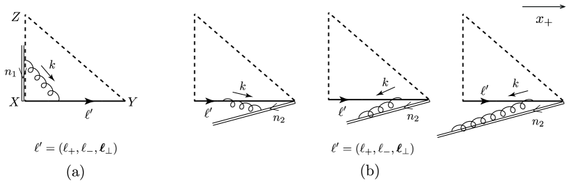
Figure 11: Diagrams that illustrate the analyticity properties of the soft function, as is explained in the text.

A light-front analysis of the denominators of the diagrams of Fig. 11(b) yields

$$-2\pi i\theta(k_{+})\theta(\ell_{+}-k_{+})\frac{1}{\ell_{+}}\frac{1}{k_{+}}\frac{1}{\ell_{+}-k_{+}}\frac{1}{\ell_{-}-(\bm{\ell}_{\perp}^{2}+m_{b}^{2})/\ell_{+}+i\varepsilon}$$

$$\quad\times\frac{1}{\ell_{-}-\bm{k}_{\perp}^{2}/k_{+}-[(\bm{\ell}_{\perp}-\bm{k}_{\perp})^{2}+m_{b}^{2}]/(\ell_{+}-k_{+})+i\varepsilon}\frac{1}{\ell_{-}-[(\bm{\ell}_{\perp}-\bm{k}_{\perp})^{2}+m_{b}^{2}]/(\ell_{+}-k_{+})+i\varepsilon}$$

$$-2\pi i\theta(-k_{+})\frac{1}{\ell_{+}}\frac{1}{k_{+}}\frac{1}{\ell_{+}-k_{+}}\frac{1}{-\bm{k}_{\perp}^{2}/k_{+}}\frac{1}{\ell_{-}-(\bm{\ell}_{\perp}^{2}+m_{b}^{2})/\ell_{+}+i\varepsilon}$$

$$\quad\times\frac{1}{\ell_{-}-[(\bm{\ell}_{\perp}-\bm{k}_{\perp})^{2}+m_{b}^{2}]/(\ell_{+}-k_{+})+i\varepsilon}.$$ (60)

In this case, there are three different contributions: the first figure shows the ordering for $k_{+}>0$, and the last two figures show the two orderings for $k_{+}<0$. In the contribution in Eq. (A) for which $k_{+}$ is positive, $k_{+}$ cannot become infinite without causing the second soft-quark line to move backward. (This leads to the constraint $\ell_{+}-k_{+}>0$.) Hence, the soft-quark lines can never have zero intermediate-state energy and the energy denominators can never vanish. In the contribution in Eq. (A) for which $k_{+}$ is negative, $-k_{+}$ can go to positive infinity without causing any of the particle lines to move backward. This is a consequence of the fact that the $n_{2}$ Wilson line can carry the momentum component $k_{+}$, but is insensitive to it. It follows that the third energy denominator can vanish when $\omega=\ell_{+}\ell_{-}\geq 0$ and, thereby, produce an imaginary part. As is usual, none of the light-front energy denominators can vanish when $\omega=\ell_{+}\ell_{-}$ is negative.

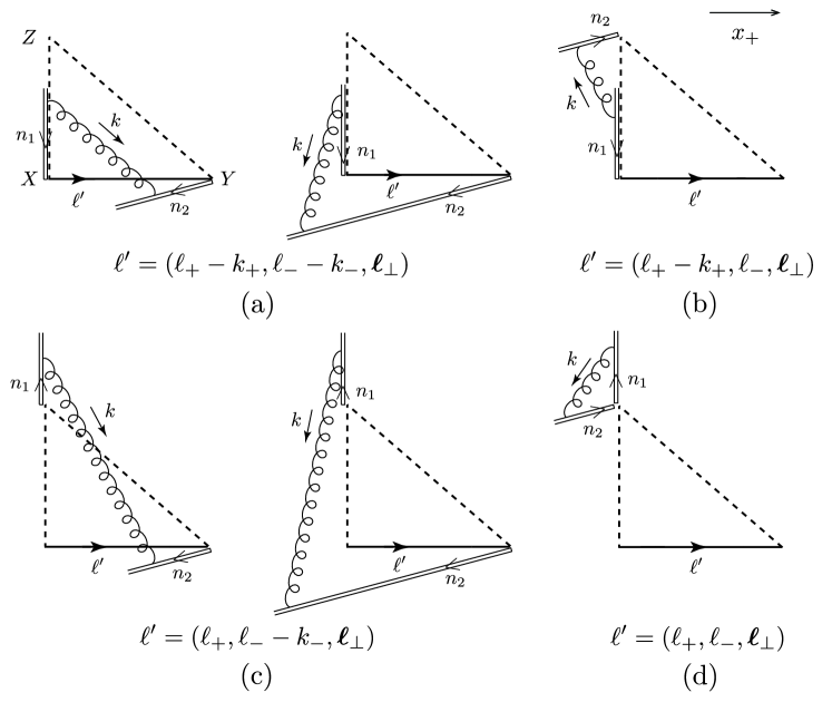
Figure 12: Additional diagrams that illustrate the analyticity properties of the soft function, as is explained in the text.

A light-front analysis of the denominators of the diagrams Fig. 12(a) yields

$$-2\pi i\theta(k_{+})\theta(\ell_{+}-k_{+})\frac{1}{k_{+}}\frac{1}{\ell_{+}-k_{+}}\frac{1}{-k_{+}+i\varepsilon}\frac{1}{\ell_{-}-\bm{k}_{\perp}^{2}/k_{+}-(\bm{\ell}_{\perp}^{2}+m_{b}^{2})/(\ell_{+}-k_{+})+i\varepsilon}$$

$$\quad\times\frac{1}{\ell_{-}-(\bm{\ell}_{\perp}^{2}+m_{b}^{2})/(\ell_{+}-k_{+})+i\varepsilon}$$

$$-2\pi i\theta(-k_{+})\frac{1}{k_{+}}\frac{1}{\ell_{+}-k_{+}}\frac{1}{-k_{+}+i\varepsilon}\frac{1}{-\bm{k}_{\perp}^{2}/k_{+}}\frac{1}{\ell_{-}-(\bm{\ell}_{\perp}^{2}+m_{b}^{2})/(\ell_{+}-k_{+})+i\varepsilon}.$$ (61)

Again, there are two different contributions: the left-hand figure shows the ordering for $k_{+}>0$, and the right-hand figure shows the ordering for $k_{+}<0$. In the contribution for which $k_{+}$ is positive, $k_{+}$ cannot become infinite without causing the soft-quark line to move backward. (This leads to the constraint $\ell_{+}-k_{+}>0$.) Hence, the soft-quark line cannot have zero intermediate-state energy, and the energy denominators can never vanish. However, for the contribution in which $k_{+}$ is negative, $-k_{+}$ can become infinite. Again, this is a consequence of the fact that the $n_{2}$ Wilson line can carry the momentum component $k_{+}$, but is insensitive to it. It follows that the second energy denominator can vanish for $\omega=\ell_{+}\ell_{-}>0$ and produce an imaginary part. Again, we see that none of the light-front energy denominators can vanish when $\omega=\ell_{+}\ell_{-}$ is negative.

A light-front analysis of the denominators of the diagram of Fig. 12(b) yields

$$2\pi i\theta(-k_{+})\frac{1}{k_{+}}\frac{1}{\ell_{+}-k_{+}}\frac{1}{-k_{+}+i\varepsilon}\frac{1}{\bm{k}_{\perp}^{2}/k_{+}}\frac{1}{\ell_{-}-(\bm{\ell}_{\perp}^{2}+m_{b}^{2})/(\ell_{+}-k_{+})+i\varepsilon}.$$ (62)

Considering the overall signs from the propagator and vertex factors from $S_{n_{2}}$ and $S^{\dagger}_{n_{2}}$, we find that there is a cancellation of the result from the diagram of Fig. 12(b) with the second term in the result from the diagram of Fig. 12(a).

A light-front analysis of the denominators of the diagrams of Fig. 12(c) yields

$$-2\pi i\theta(k_{+})\frac{1}{\ell_{+}}\frac{1}{k_{+}}\frac{1}{-k_{+}+i\varepsilon}\frac{1}{\ell_{-}-(\bm{\ell}_{\perp}^{2}+m_{b}^{2})/\ell_{+}-\bm{k}_{\perp}^{2}/k_{+}+i\varepsilon}\frac{1}{\ell_{-}-(\bm{\ell}_{\perp}^{2}+m_{b}^{2})/\ell_{+}+i\varepsilon}$$

$$-2\pi i\theta(-k_{+})\frac{1}{\ell_{+}}\frac{1}{k_{+}}\frac{1}{-k_{+}+i\varepsilon}\frac{1}{-\bm{k}_{\perp}^{2}/k_{+}}\frac{1}{\ell_{-}-(\bm{\ell}_{\perp}^{2}+m_{b}^{2})/\ell_{+}+i\varepsilon}.$$ (63)

There are two different contributions: the left-hand figure shows the ordering for $k_{+}>0$, and the right-hand figure shows the ordering for $k_{+}<0$. In both cases, the longitudinal momentum $k_{+}$ does not appear in the soft-quark line and, so, its intermediate-state energy can never vanish. Consequently, the energy denominators cannot vanish unless $\omega=\ell_{+}\ell_{-}$ is greater than or equal to $m_{b}^{2}$.

Finally, a light-front analysis of the denominators of diagram of Fig. 12(d) yields

$$2\pi i\theta(-k_{+})\frac{1}{\ell_{+}}\frac{1}{k_{+}}\frac{1}{-k_{+}+i\varepsilon}\frac{1}{\bm{k}_{\perp}^{2}/k_{+}}\frac{1}{\ell_{-}-(\bm{\ell}_{\perp}^{2}+m_{b}^{2})/\ell_{+}+i\varepsilon}.$$ (64)

Again, the longitudinal momentum $k_{+}$ does not appear in the soft-quark line, and, so, its intermediate-state energy can never vanish. Consequently, this expression has a vanishing light-front energy denominator only if $\omega=\ell_{+}\ell_{-}$ is greater than or equal to $m_{b}^{2}$.

From the foregoing examples in light-front perturbation theory, we have seen that, owing to the unorthodox momentum routing in the soft function or to the presence of an $n_{2}$ Wilson line, a soft-quark line can carry an infinite $+$ longitudinal momentum without causing any particle line to move backward. This leads to a vanishing of the intermediate-state energy of the soft-quark line, and it is the mechanism by which a vanishing light-front energy denominator can appear for $\omega\geq 0$. Hence, in consequence of the $i\varepsilon$ in the energy denominator, the soft function has a cut that runs from $\omega=-i\varepsilon$ just below the real axis to infinity. On the other hand, owing to the fact that none of the intermediate-state particle energies can be negative, energy denominators can never vanish if $\omega<0$, and the soft function is analytic everywhere in the complex $\omega$ plane except for the cut along the positive real axis.

References

- (1) M. Spira, A. Djouadi, D. Graudenz and P. M. Zerwas, Higgs boson production at the LHC, Nucl. Phys. B 453, 17-82 (1995) [arXiv:hep-ph/9504378].
- (2) M. Beneke, G. Buchalla, M. Neubert and C. T. Sachrajda, QCD factorization for exclusive, nonleptonic B meson decays: General arguments and the case of heavy light final states, Nucl. Phys. B 591 (2000), 313-418 [arXiv:hep-ph/0006124].
- (3) M. Beneke, T. Feldmann and D. Seidel, Systematic approach to exclusive , decays, Nucl. Phys. B 612 (2001), 25-58 [arXiv:hep-ph/0106067].
- (4) M. Beneke, G. Buchalla, M. Neubert and C. T. Sachrajda, QCD factorization in B — pi K, pi pi decays and extraction of Wolfenstein parameters, Nucl. Phys. B 606 (2001), 245-321 [arXiv:hep-ph/0104110].
- (5) M. Beneke and T. Feldmann, Factorization of heavy to light form-factors in soft collinear effective theory, Nucl. Phys. B 685 (2004), 249-296 [arXiv:hep-ph/0311335].
- (6) M. Beneke and M. Neubert, QCD factorization for B — PP and B — PV decays, Nucl. Phys. B 675 (2003), 333-415 [arXiv:hep-ph/0308039].
- (7) Y. Jia, J. X. Wang and D. Yang, Bridging light-cone and NRQCD approaches: asymptotic behavior of electromagnetic form factor, JHEP 10 (2011), 105 [arXiv:1012.6007 [hep-ph]].
- (8) M. Benzke, S. J. Lee, M. Neubert and G. Paz, Factorization at Subleading Power and Irreducible Uncertainties in Decay, JHEP 08 (2010), 099 [arXiv:1003.5012 [hep-ph]].
- (9) G. T. Bodwin, H. S. Chung and J. Lee, Double logarithms in , Phys. Rev. D 90 (2014) no.7, 074028 [arXiv:1406.1926 [hep-ph]].
- (10) M. Beneke, A. Broggio, S. Jaskiewicz and L. Vernazza, Threshold factorization of the Drell-Yan process at next-to-leading power, JHEP 07 (2020), 078 [arXiv:1912.01585 [hep-ph]].
- (11) I. Moult, I. W. Stewart and G. Vita, Subleading Power Factorization with Radiative Functions, JHEP 11 (2019), 153 [arXiv:1905.07411 [hep-ph]].
- (12) I. Moult, I. W. Stewart, G. Vita and H. X. Zhu, The Soft Quark Sudakov, JHEP 05 (2020), 089 [arXiv:1910.14038 [hep-ph]].
- (13) M. van Beekveld, W. Beenakker, E. Laenen and C. D. White, Next-to-leading power threshold effects for inclusive and exclusive processes with final state jets, JHEP 03 (2020), 106 [arXiv:1905.08741 [hep-ph]].
- (14) Z. L. Liu and M. Neubert, Factorization at subleading power and endpoint-divergent convolutions in decay, JHEP 04, 033 (2020) [arXiv:1912.08818 [hep-ph]].
- (15) M. I. Kotsky and O. I. Yakovlev, On the resummation of double logarithms in the process Higgs — gamma gamma, Phys. Lett. B 418, 335-344 (1998) [arXiv:hep-ph/9708485].
- (16) R. Akhoury, H. Wang and O. I. Yakovlev, On the Resummation of large QCD logarithms in Higgs — gamma gamma decay, Phys. Rev. D 64, 113008 (2001) [arXiv:hep-ph/0102105].
- (17) J. Wang, Resummation of double logarithms in loop-induced processes with effective field theory, [arXiv:1912.09920 [hep-ph]].
- (18) Z. L. Liu, B. Mecaj, M. Neubert and X. Wang, Factorization at Subleading Power and Endpoint Divergences in Soft-Collinear Effective Theory, [arXiv:2009.04456 [hep-ph]].
- (19) Z. L. Liu, B. Mecaj, M. Neubert and X. Wang, Factorization at Subleading Power and Endpoint Divergences in Decay: II. Renormalization and Scale Evolution, [arXiv:2009.06779 [hep-ph]].
- (20) C. W. Bauer, S. Fleming, D. Pirjol and I. W. Stewart, An Effective field theory for collinear and soft gluons: Heavy to light decays, Phys. Rev. D 63, 114020 (2001) [arXiv:hep-ph/0011336].
- (21) C. W. Bauer, D. Pirjol and I. W. Stewart, Soft collinear factorization in effective field theory, Phys. Rev. D 65, 054022 (2002) [arXiv:hep-ph/0109045].
- (22) M. Beneke and T. Feldmann, Multipole expanded soft collinear effective theory with nonAbelian gauge symmetry, Phys. Lett. B 553, 267-276 (2003) [arXiv:hep-ph/0211358].
- (23) C. W. Bauer, S. Fleming, D. Pirjol, I. Z. Rothstein and I. W. Stewart, Hard scattering factorization from effective field theory, Phys. Rev. D 66, 014017 (2002) [arXiv:hep-ph/0202088].
- (24) M. Beneke, A. P. Chapovsky, M. Diehl and T. Feldmann, Soft collinear effective theory and heavy to light currents beyond leading power, Nucl. Phys. B 643, 431-476 (2002) [arXiv:hep-ph/0206152].
- (25) Z. L. Liu, B. Mecaj, M. Neubert, X. Wang and S. Fleming, Renormalization and Scale Evolution of the Soft-Quark Soft Function, JHEP 07, 104 (2020) [arXiv:2005.03013 [hep-ph]].
- (26) V. Del Duca, High-energy Bremsstrahlung Theorems for Soft Photons, Nucl. Phys. B 345 (1990), 369-388.
- (27) D. Bonocore, E. Laenen, L. Magnea, S. Melville, L. Vernazza and C. D. White, A factorization approach to next-to-leading-power threshold logarithms, JHEP 06 (2015), 008 [arXiv:1503.05156 [hep-ph]].
- (28) D. Bonocore, E. Laenen, L. Magnea, L. Vernazza and C. D. White, Non-abelian factorisation for next-to-leading-power threshold logarithms, JHEP 12 (2016), 121 [arXiv:1610.06842 [hep-ph]].
- (29) E. Lunghi, D. Pirjol and D. Wyler, Factorization in leptonic radiative B e decays, Nucl. Phys. B 649 (2003), 349-364 [arXiv:hep-ph/0210091].
- (30) S. W. Bosch, R. J. Hill, B. O. Lange and M. Neubert, Factorization and Sudakov resummation in leptonic radiative B decay, Phys. Rev. D 67 (2003), 094014 [arXiv:hep-ph/0301123].
- (31) Y. M. Wang, Factorization and dispersion relations for radiative leptonic decay, JHEP 09, 159 (2016) [arXiv:1606.03080 [hep-ph]].
- (32) Y. M. Wang and Y. L. Shen, Subleading-power corrections to the radiative leptonic decay in QCD, JHEP 05, 184 (2018) [arXiv:1803.06667 [hep-ph]].
- (33) A. V. Manohar, T. Mehen, D. Pirjol and I. W. Stewart, Reparameterization invariance for collinear operators, Phys. Lett. B 539 (2002), 59-66 [arXiv:hep-ph/0204229].
- (34) J. C. Collins, D. E. Soper and G. F. Sterman, Factorization of Hard Processes in QCD, Adv. Ser. Direct. High Energy Phys. 5, 1-91 (1989) [arXiv:hep-ph/0409313].
- (35) G. Grammer, Jr. and D. R. Yennie, Improved treatment for the infrared divergence problem in quantum electrodynamics, Phys. Rev. D 8, 4332-4344 (1973).
- (36) J. Collins, “Foundations of perturbative QCD,” Camb. Monogr. Part. Phys. Nucl. Phys. Cosmol. 32 (2011), 1-624, Sec. 7.2.3.
- (37) S. J. Chang and S. K. Ma, Feynman rules and quantum electrodynamics at infinite momentum, Phys. Rev. 180 (1969), 1506-1513.
- (38) J. B. Kogut and D. E. Soper, Quantum Electrodynamics in the Infinite Momentum Frame, Phys. Rev. D 1 (1970), 2901-2913.
- (39) T. M. Yan, Quantum field theories in the infinite momentum frame. 4. Scattering matrix of vector and Dirac fields and perturbation theory, Phys. Rev. D 7 (1973), 1780-1800.