Stochastic enzyme kinetics and the quasi-steady-state reductions: Application of the slow scale linear noise approximation à la Fenichel

Abstract

The linear noise approximation models the random fluctuations from the mean-field model of a chemical reaction that unfolds near the thermodynamic limit. Specifically, the fluctuations obey a linear Langevin equation up to order $\Omega^{-1/2}$, where $\Omega$ is the size of the chemical system (usually the volume). In the presence of disparate timescales, the linear noise approximation admits a quasi-steady-state reduction referred to as the slow scale linear noise approximation (ssLNA). Curiously, the ssLNAs reported in the literature are slightly different. The differences in the reported ssLNAs lie at the mathematical heart of the derivation. In this work, we derive the ssLNA directly from geometric singular perturbation theory and explain the origin of the different ssLNAs in the literature. Moreover, we discuss the loss of normal hyperbolicity and we extend the ssLNA derived from geometric singular perturbation theory to a non-classical singularly perturbed problem. In so doing, we disprove a commonly-accepted qualifier for the validity of stochastic quasi-steady-state approximation of the Michaelis–Menten reaction mechanism.

1 Introduction

The set of elementary reactions that comprise a chemical system often occur at disproportionate rates. From the chemical physics point of view, chemical systems whose elementary reaction rates are disparate constitute a multiscale process. From a modeling point of view, multiscale reactions are highly advantageous, since the presence of widely separated timescales permits a reduction in the number of mathematical equations required to model the reaction over slow (long) timescales.

In the deterministic regime, near the thermodynamic limit, chemical equations can be accurately modeled with a system of nonlinear ordinary differential equations. The reduction of deterministic models is generally achieved through the application of Tikhonov’s theorem [1] and Fenichel theory [2, 3]. Several analyses of enzyme-catalyzed reactions have made good use of singular perturbation theory to generate approximations referred to as quasi-steady-state (QSS) approximations or reductions [4, 5]. In fact, over the last decade, much progress has been made in developing and applying the formalism of Fenichel theory to chemical kinetics, and the culmination of the recent literature has turned up some surprising results. First and foremost, the advent of Tikhonov-Fenichel parameter value (TFPV) theory, developed extensively by Goeke et al. [6, 7], has rigorously demonstrated that not all QSS reductions emerge as a result of a singular perturbation scenario, despite what scaling and numerical simulations might suggest [8, 9]. TFPV theory has also enhanced our understanding of the singular perturbation structure (when applicable) to pertinent reaction models, which has led to the discovery of bifurcations and other interesting phenomena present in the singular vector fields of the model equations [5]. Most surprising, however, is the revelation that traditional scaling methods may lead to erroneous conclusions concerning the mathematical origin and justification of QSS reduction in chemical kinetics (see, for example, Goeke et al. [10], Section 4, as well as Eilertsen et al. [9]).

Given the recent developments in the deterministic theory of QSS reduction, the natural question to ask is: Do any of these developments have something important to say about model reduction in the stochastic realm? Model reduction is more challenging in the stochastic regime, but rigorous reduction methods that leverage the presence of disparate timescales do exist (see, for example, [11, 12, 13]). The focus of this paper is on the application of QSS reduction in the linear noise regime, where stochastic fluctuations from the deterministic mean-field model are governed by a linear Langevin equation called the linear noise approximation (LNA). The general methodology for QSS reduction in the LNA regime, called the slow scale linear noise approximation (ssLNA), is by Thomas et al. [14], Pahlajani et al. [15], and Herath and Del Vecchio [16]. Interestingly, the reported ssLNAs are slightly different, and this raises the question: Where do these differences come from, and are they critical? The intent of this paper is three-fold: (i) to explain why different ssLNAs exist in the literature, (ii) to introduce recent developments of deterministic QSS theory to the stochastic community, and (iii) to demonstrate techniques to extend the ssLNA to specific non-classical singularly-perturbed problems. In what follows, we revisit the mathematical formalism of geometric singular perturbation theory (GSPT) and derive the ssLNA directly from GSPT. We discuss the role of TFPV theory in the applicability of GSPT, and demonstrate where the differences emerge between the GSPT-derived ssLNA and the ssLNAs of Thomas et al. [14], Pahlajani et al. [15], and Herath and Del Vecchio [16]. We also discuss the role of the GSPT-derived ssLNA in the QSS reduction of the chemical master equation (CME) and use it to debunk a well-established result in the literature.

2 Singular perturbations and Fenichel Theory: A brief introduction

In this section, we give a very brief overview of Fenichel theory as it applies to singular perturbations by shadowing Wechselberger [17, Chapter 3]. However, the results were originally obtained by Fenichel [3, Section 5]. A detailed mathematical expose on Fenichel reduction and its applicability in enzyme kinetics can be found in [8, 10, 18].

2.1 Coordinate-free slow manifold projection

Fenichel theory is concerned with the persistence of normally hyperbolic invariant manifolds with respect to a perturbation. Dynamical systems subject to a small perturbation are of the general form

$$\dot{z}=w(z)+\varepsilon G(z,\varepsilon)$$ (1)

where $0<\varepsilon\ll 1$. The stationary points of the unperturbed vector field, $w(z)$, determine the classification of the perturbation problem. If the perturbation is singular, then there exists a set, $S$, comprised of non-isolated equilibrium points:

$$S:=\{z\in\mathbb{R}^{n}:w(z)=0\}.$$

Fenichel reduction applies to compact subsets, $\mathcal{S}_{0}\subseteq S$ that are differentiable manifolds (with a possible boundary). The compactness requirement of $\mathcal{S}_{0}$ is generally easy to satisfy in chemical kinetics: due to conservation laws, phase-space trajectories remain within a bounded, positively invariant set, $\Lambda$. If $S_{0}$ is an embedded $k$-dimensional submanifold of $\mathbb{R}^{n}$, then

$$\text{rank}\;Dw(z)=n-k\quad\forall z\in S_{0}.$$

Furthermore, if the algebraic and geometric multiplicity of the zero eigenvalue are both equal to $k$, then

$$T_{z}S_{0}:=\{x\in\mathbb{R}^{n}:Dw(z)\cdot x=0\}=\ker Dw(z)\quad\forall z\in S_{0},$$ (2)

and there is continuous splitting,

$$\mathbb{R}^{n}:=\ker Dw(z)\oplus\text{Image}\;Dw(z)$$ (3)

for all $z\in S_{0}$. Perturbing the vector field by setting $0<\varepsilon\ll 1$ results in the formation of an invariant, slow manifold, $M$. If the real parts of the $n-k$ non-zero eigenvalues of $Dw(z)$ are strictly less than zero, then $M$ will attract nearby trajectories at an exponentially fast rate. Projecting the perturbation, $\varepsilon G(z,0)$, onto the tangent space of $S_{0}$ results in a reduced equation (called a QSS approximation) that captures the long-time behavior of the system.

The decomposition (3) implies the existence of a projection operator, $\Pi^{S_{0}}$, that maps to $\ker Dw(z)$

$$\Pi^{S_{0}}:\mathbb{R}^{n}\mapsto T_{z}S_{0}\quad\forall x\in S_{0}.$$ (4)

The explicit form of $\Pi^{S_{0}}$ is obtained by exploiting the fact that $w(z)$ factors (locally) as

$$w(z):=N(z)\mu(z),\quad N(z)\in\mathbb{R}^{n\times(n-k)},\quad\mu(z)\in\mathbb{R}^{n-k}.$$ (5)

The columns of $N$ comprise a basis for the range of the Jacobian, $Dw(z)$, and the zero level set of $\mu(z)$ is identically $S_{0}$. Since $\text{rank}\;Dw(z)=n-k$, and the zero set of $\mu:\mathbb{R}^{n}\mapsto\mathbb{R}^{n-k}$ corresponds to $S_{0}$ (a submanifold of $\mathbb{R}^{n}$), we have that, for all $z\in S_{0}$, $N(z)$ has full (column) rank, and $D\mu(z)$ has full (row) rank:

rank $$N(z)=\;n-k,$$ (6a)

rank $$D\mu(z)=n-k.$$ (6b)

The row vectors of $D\mu(z)$ form a basis for the orthogonal complement of $\ker Dw(z)$. Since projection operators are uniquely determined by their range and the orthogonal complement of their kernel, the operator $\Pi^{S_{0}}$ is

$$\Pi^{S_{0}}:=I-N(D\mu N)^{-1}D\mu$$ (7)

which is an oblique projection operator (see Figure 1 for a geometric interpretation of $\Pi^{S_{0}}$).

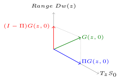
Figure 1: The geometry of $\Pi^{S_{0}}$. The projection matrix, labeled here as $\Pi$, defines an oblique projection: while ${\rm Range}\;Dw(z)\cap\ker Dw(z)=\{0\}$ for $z\in S_{0}$, ${\rm Range}\;Dw(z)$ is not necessarily orthogonal to $\ker Dw(z)$.

Once the projection operator is constructed, the reduced equation is formulated by projecting the perturbation, $G(z,0)$, onto $\ker Dw(z)$:

$$\dot{z}=\Pi^{S_{0}}G(z,0)|_{z\in S_{0}}.$$

3 Singular perturbation reduction in biochemical kinetics: Didactic examples

In this section, we compute several QSS reductions of the MM reaction mechanism. We introduce the mass action equations of the deterministic MM reaction mechanism and discuss the computation of QSS reductions directly from Fenichel theory without a priori non-dimensionalization. Several QSS reductions are computed, including the standard QSS approximation (sQSSA) and the quasi-equilibrium approximation (QEA).

3.1 The Michaelis–Menten reaction mechanism

The MM reaction consists of three elementary reactions: the binding of a substrate molecule, S, with an enzyme molecule, E, leading to the formation of an intermediate complex molecule, C. The complex molecule can disassociate back into unbound enzyme and substrate molecules, or it disassociates into a product molecule, P, and an enzyme molecule. The chemical equation is given by

$$\ce{S+E<=>[k_{1}][k_{-1}]C->[k_{2}]E+P},$$ (8)

where $k_{1}$, $k_{-1}$ and $k_{2}$ are deterministic rate constants.

The mass action equations that describe the kinetics of (8) in the thermodynamic limit constitute a two-dimensional system of nonlinear ordinary differential equations,

$$\dot{s} =-k_{1}(e_{T}-c)s+k_{-1}c,$$ (9a)

$$\dot{c} =k_{1}(e_{T}-c)s-(k_{-1}+k_{2})c,$$ (9b)

where lowercase $s$, $c$, $e$ and $p$ denote the concentrations of S, C, E and P, respectively. Once the temporal dynamics of $s$ and $c$ are known, the evolution of product is recovered from

$$\dot{p}=k_{2}c.$$ (10)

The temporal concentration of enzyme, $e$, is computed from $e_{T}-c$, where $e_{T}$ is a conserved quantity, the total enzyme concentration, and accounts for the concentration of both bound and unbound enzyme molecules. A second conservation law is obtained from the addition of (9a)–(10), $\dot{s}+\dot{c}+\dot{p}=0$, yielding the conservation of substrate:

$$s_{T}=s+c+p.$$ (11)

Unless otherwise stated, we will take $s(0)=s_{T}$ in the analysis that follows, which implies $c(0)=p(0)=0$.

3.2 Tikhonov-Fenichel Parameter Value Theory

It is possible (and convenient) to compute QSS reductions directly from the dimensional equation. This a result of the TFPV theory developed by Goeke et al. [6, 19, 20], which we briefly outline here.

In physical applications, most dynamical systems depend on an $m$-tuple of parameters, $\pi\in\mathbb{R}^{m}$:

$$\dot{z}=f(z,\pi),\quad z\in\mathbb{R}^{n},\;\;\pi\in\mathbb{R}^{m},\;\;f:\mathbb{R}^{n}\times\mathbb{R}^{m}\mapsto\mathbb{R}^{n}.$$

A TFPV value is a point, $\widehat{\pi}$, in parameter space for which the vector field, $f(z,\widehat{\pi})$, contains a normally hyperbolic and attracting critical manifold.

As an example, the MM reaction mechanism mass action equations depend on the parameters $\pi=(e_{T},k_{1},k_{-1},k_{2})^{tr.}$, where $tr.$ denotes transpose. There are three engaging TFPV values associated with the MM reaction mechanism:

$$\widehat{\pi}_{1}:=(0,k_{1},k_{-1},k_{2})^{tr.},$$

$$\widehat{\pi}_{2}:=(e_{T},0,k_{-1},k_{2})^{tr.},$$

$$\widehat{\pi}_{3}:=(e_{T},k_{1},k_{-1},0)^{tr.}.$$

Singular perturbation theory applies to vector fields that are sufficiently close to the TFPVs. Thus, the QSS reductions that are constructed by projecting onto the tangent space of a critical manifold associated with the TFPVs will be valid for $\pi$ sufficiently close $\widehat{\pi}_{i}$. Consequently, we will consider parameter values close to TFPVs:

$${\pi}_{1}:=(\varepsilon\widehat{e}_{T},k_{1},k_{-1},k_{2})^{tr.},$$

$${\pi}_{2}:=(e_{T},\varepsilon\widehat{k}_{1},k_{-1},k_{2})^{tr.},$$

$${\pi}_{3}:=(e_{T},k_{1},k_{-1},\varepsilon\widehat{k}_{2})^{tr.},$$

where $\varepsilon$ is very small but positive, and $\widehat{e}_{T}$, $\widehat{k}_{1}$ and $\widehat{k}_{2}$ are of unit magnitude and simply encode the units of $e_{T}$, $k_{1}$ and $k_{2}$, respectively. As we demonstrate in the subsection that follows, this notation enables the computation of QSS reductions without the need to non-dimensionalize the mass action equations.

3.3 Fenichel reduction: The sQSSA of the MM reaction mechanism

To extract a reduced model from (9), we begin with the assumption that $e_{T}$ is small and therefore $\pi$ is close to $\widehat{\pi}_{1}$. Consequently, we rescale $e_{T}$ as $e_{T}\mapsto\varepsilon\widehat{e}_{T}$, where $0<\varepsilon\ll 1$ (again, this notation really just serves as a reminder that $e_{T}$ is small). In $(s,c)$ coordinates, we have $z:=(s\;\;c)^{T}$, and in perturbation form, the mass action equations (9) are

$$\dot{z}=w(z)+\varepsilon G(z,\varepsilon),\quad w(z):=\begin{pmatrix}k_{1}cs+k_{-1}c\\ -k_{1}cs-(k_{-1}+k_{2})c\end{pmatrix},\quad G(z,\varepsilon):=\begin{pmatrix}-k_{1}\widehat{e}_{T}s\\ \;\;k_{1}\widehat{e}_{T}s\end{pmatrix}.$$ (14)

The singular problem recovered by setting $\varepsilon=0$ so that $\pi=\widehat{\pi}_{1}$ yields a critical manifold of equilibria

$$S_{0}:=\{(s,c)\in\mathbb{R}^{2}:c=0,\quad 0\leq s\leq s_{T}\}.$$ (15)

It is straightforward to verify that $S_{0}$ is normally hyperbolic. Moreover, since the non-trivial eigenvalue of the Jacobian, $\lambda_{MM}$, is strictly less than zero

$$\lambda_{MM}:=-(k_{1}s+k_{-1}+k_{2})$$

the critical manifold is attractive.

Since $S_{0}$ is normally hyperbolic and attracting, we proceed to compute $\Pi^{S_{0}}$. The factorization of $w(z)$ is straightforward to compute

$$w(z)=N(s,c)\mu(s,c),\quad\text{with}\quad N(s,c):=\begin{pmatrix}k_{1}s+k_{-1}\\ -k_{1}s-k_{-1}-k_{2}\end{pmatrix},\quad\text{and}\quad\mu(s,c):=c,$$ (16)

as is the derivative of $\mu(s,c)=c$:

$$D\mu(s,c)=(0\;\;1).$$ (17)

Putting the pieces together, the projection operator $\Pi^{S_{0}}$ is

$$\Pi^{S_{0}}:=\begin{pmatrix}1&\gamma(s)\\ 0&0\end{pmatrix},\quad\gamma(s):=\cfrac{K_{S}+s}{K_{M}+s},$$ (18)

where $K_{S}=k_{-1}/k_{1}$ and $K_{M}=(k_{-1}+k_{2})/k_{1}$. The corresponding QSS approximation is

$$\dot{s}=\Pi^{S_{0}}G(s,c,0)|_{c=0}:=-\cfrac{k_{2}e_{T}s}{K_{M}+s},$$ (19)

which is the sQSSA.

Remark 1

Note that the sQSSA (19) is not the result of singular perturbation problem that is in standard form

$$\dot{x} =\varepsilon f(x,y,\varepsilon),$$

$$\dot{y} =\;\;g(x,y,\varepsilon).$$

This is contrary to the justification established from scaling analyses that utilize non-dimensionalization (see, Heineken et al. [21], Segel and Slemrod [22]).

3.4 Fenichel reduction: The QEA

In addition to the sQSSA, the QEA is a QSS reduction that is valid in the limit of slow product formation that occurs when $\pi$ is close to $\widehat{\pi}_{3}$. Rescaling $k_{2}$ as $k_{2}\mapsto\varepsilon\widehat{k}_{2}$, the mass action system

$$\dot{s} =-k_{1}(e_{T}-c)s+k_{-1}c,$$ (21a)

$$\dot{c} =k_{1}(e_{T}-c)s-k_{-1}c-\varepsilon\widehat{k}_{2}c,$$ (21b)

has a critical manifold of equilibria in the singular limit that coincides with $\pi=\widehat{\pi}_{3}:$

$$S:=\bigg{\{}(s,c)\in\mathbb{R}^{2}:c=\cfrac{e_{T}s}{K_{S}+s}\bigg{\}},$$ (22)

which is identical to the $s$-nullcline. The QEA in $(s,c)$ coordinates is well understood but trickier than the sQSSA. The consequence is that there can be noticeable depletion of $s$ during the approach to the slow manifold unless $e_{T}\ll K_{M}+s_{T}$ [23, 22]. We will not rehash the details here, but state the main results also found in [6, 17]. The projection matrix, $\Pi^{S_{0}}$, and perturbation, $G(s,c,0)$, are given by

$$\Pi^{S_{0}}:=\cfrac{1}{(e_{T}-c+K_{S}+s)}\begin{pmatrix}(K_{S}+s)&(K_{S}+s)\\ (e_{T}-c)&(e_{T}-c)\end{pmatrix},\qquad G(s,c,0):=-\begin{pmatrix}0\\ \widehat{k}_{2}c\end{pmatrix},$$ (23)

and corresponding QSS reduction for $s$ is

$$\dot{s}=-\cfrac{k_{2}e_{T}s(K_{S}+s)}{e_{T}K_{S}+(K_{S}+s)^{2}},\quad\dot{p}=\cfrac{k_{1}k_{2}e_{T}s}{k_{1}s+k_{-1}}.$$ (24)

3.5 Fenichel reduction: The reverse QSSA

The reverse QSSA (rQSSA) was originally defined by Segel and Slemrod [22] as a perturbation problem, and later investigated in detail by Schnell and Maini [24]. To preface the derivation of the rQSSA as a Fenichel reduction, we remark that there are two common conditions that emerge in biochemical applications:

1. $ND\mu(z)$ vanishes (or changes rank) at at least one point belonging to the critical set. This happens, for example, if $D\mu(z)=0$ at some point belonging to the set $\mu(z)=0$.

2. The zero eigenvalue of the Jacobian evaluated at at least one point in $S_{0}$ has an algebraic multiplicity that is greater than the geometric multiplicity (the splitting (3) does not hold at such points).

The rQSSA is valid for small $k_{-1}$ and small $k_{2}$, and is of the variety 1. In perturbation form this corresponds to

$$\dot{s} =-k_{1}(e_{T}-c)s+\varepsilon\widehat{k}_{-1}c,$$ (25a)

$$\dot{c} =k_{1}(e_{T}-c)s-\varepsilon(\widehat{k}_{-1}+\widehat{k}_{2})c.$$ (25b)

The critical set is given by,

$$S_{0}:=\{(s,c)\in\mathbb{R}^{2}_{\geq 0}:c=e_{T},0\leq s\leq s_{T}\}\cup\{(s,c)\in\mathbb{R}^{2}_{\geq 0}:s=0,0\leq c\leq e_{T}\}.$$ (26)

The rank of the Jacobian along $S_{0}$ is not constant

$${\rm rank}\;\;Dw(s,c) =0,\;\;\text{if}\;\;(s,c)=(0,e_{T}),$$

$${\rm rank}\;\;Dw(s,c) =1,\;\;\text{otherwise},$$

and thus TFPV theory does not apply. However, observe that the compact submanifolds

$$S_{a}^{r} :=\{(s,c)\in\mathbb{R}^{2}_{\geq 0}:c=e_{T},\;\;\varrho\leq s\leq s_{T}\},\qquad\;0<\varrho,$$

$$S_{a}^{b} :=\{(s,c)\in\mathbb{R}^{2}_{\geq 0}:s=0,\;\;0\leq c\leq e_{T}-\kappa\},\quad 0<\kappa<e_{T}$$

are normally hyperbolic and attracting. When $s(0)>0$, trajectories will initially approach and follow $S_{a}^{r}$ before eventually following $S_{a}^{b}$. In fact, a quick analysis reveals the existence of a transcritical bifurcation (see Figure 2).

Figure 2: A dynamic transcritical bifurcation occurs in the singular limit corresponding to $k_{2}=k_{-1}=0$ of the MM reaction mechanism. At $S^{\star}$ the Jacobian has a double-zero eigenvalue. Along the dashed lines the Jacobian has one zero eigenvalue and one positive eigenvalue. Along the solid lines the Jacobian has one zero eigenvalue and one negative eigenvalue. At the bifurcation point $S^{\star}=(0,e_{T})$, the lines $S_{a}^{r}\cup S_{r}^{l}$ and $S_{r}^{t}\cup S_{a}^{b}$ intersect and exchange stability.

By the projection methods above, it is straightforward to show that the QSS reductions obtained via projection onto $T_{z}S_{a}^{r}$ and $T_{z}S_{a}^{b}$ are, respectively:

$$\dot{p} =k_{2}e_{T},\qquad\qquad\;\;0\leq p<s_{T}-e_{T}$$ (29a)

$$\dot{p} =k_{2}(s_{T}-p),\qquad s_{T}-e_{T}<p\leq s_{T}.$$ (29b)

As a concluding remark, note that we have successfully computed QSS reductions without a priori scaling and non-dimensionalization of the mass action equations. The ability to compute QSS reductions directly from the dimensional equations is a result of the TFPV theory developed by Goeke et al. [7, 6], which we have utilized here.

4 Stochastic chemical kinetics: Expansions, reductions, and approximations

In this section, we discuss QSS reduction in the stochastic regime. We introduce the CME and the derivation of the LNA via the $\Omega$–expansion. We conclude with a review of the ssLNA as derived by Thomas et al. [14] and Pahlajani et al. [15], and we compare it to the GSPT-derived ssLNA.

4.1 Stochastic chemical kinetics far from the thermodynamic limit: The master equation

Under physical conditions, a reaction occurs within a bounded volume, $\Omega$. If the number of molecules in the system is finite, the reaction will always exhibit fluctuations. In fact, in the presence of random fluctuations and intrinsic noise, stochastic models provide a more physically realistic description of the kinetics when a system is far from the thermodynamic limit since the time interval between successive reactions becomes a random variable. The appropriate mathematical model depends on how “close” the system is to the thermodynamic limit.

If the chemical reaction consists of “$R$” elementary reactions, and the mixture is homogeneous and not diffusion limited then, far from the thermodynamic limit, the probability of finding the system in state ${Z}$ at time $t$ can be obtained from the solution to CME (see, [25] and [26] for details),

$$\cfrac{\partial P(Z,t)}{\partial t}=\sum_{j=1}^{R}a_{j}(Z-{\nu}_{j})P({Z}-{\nu}_{j},t)-a_{j}({Z})P({Z},t),$$ (30)

where ${\nu}_{j}$ are the stoichiometric vectors that correspond to the $jth$ elementary reaction. If the system is in state $Z$ when the $jth$ reaction occurs, then the new state of the system will be ${Z}+{\nu}_{j}$. The functions $a_{j}$ are called propensity functions. Dynamically the state of the system at time $t$ is ${Z}$, and it moves from state ${Z}$ to the state ${Z}+{\nu}_{j}$ within the infinitesimal window $[t,t+\text{d}t)$ with the probability

$$P({Z}+{\nu}_{j},t+\text{d}t|{Z},t)=a_{j}({Z})\text{d}t.$$ (31)

The conditional probability (31) of jumping into the state ${Z}+{\nu}_{j}$ depends only on the present state of the system, which is called the Markov property.

The CME is possibly the most fundamental description of a chemical reaction. The difficulty is that closed-form solutions are rarely attainable. This begs question: Is it possible to derive physical models that exhibit stochasticity, but are nevertheless easier to analyze? The answer is yes, but the cost is that simplified models are usually only valid in monostable systems near the thermodynamic limit. The LNA is of this variety.

4.2 Approaching the thermodynamic limit: the LNA

To introduce the LNA, it is helpful to express the mass action equations in the form

$$\dot{z}=\mathcal{S}q,\quad F:=diag(q)$$ (32)

where $\mathcal{S}$ is the stoichiometric matrix, and $q$ is the main diagonal of the matrix $F$, whose diagonal components correspond to the elementary reactions of the chemical system. For example, the MM reaction mechanism (8) consists of three elementary reactions: the formation of complex, the disassociation of complex into S and E, and the disassociation of complex into E and P. Hence, the mass action system in form (32) is

$$\begin{pmatrix}\dot{s}\\ \dot{c}\end{pmatrix}=\begin{pmatrix}-1&\;\;\;1&\;\;\;0\\ \;\;\;1&-1&-1\end{pmatrix}\begin{pmatrix}k_{1}(e_{T}-c)s\\ k_{-1}c\\ k_{2}c\end{pmatrix}:=\mathcal{S}q.$$ (33)

To formally derive the LNA, one starts with the operator form of the CME,

$$\cfrac{\partial P({Z},t)}{\partial t}=\Omega\sum_{j=1}^{R}\bigg{(}\prod_{i=1}^{m}\mathbb{E}^{\mathcal{S}_{ij}}-1\bigg{)}a_{j}({z})P({Z},t),$$ (34)

where $z=Z/\Omega$ and $\mathbb{E}^{\mathcal{S}_{ij}}$ is the step operator:

$$\ \mathbb{E}^{-\mathcal{S}_{ij}}a({Z})=a(\mathbb{E}^{-\mathcal{S}_{ij}}{Z})=a({Z}-\mathcal{S}_{ij}{e}_{i}).$$ (35)

Inserting the ansatz ${Z}=\Omega{z}+\Omega^{1/2}{X}$ into (34) and expanding (34) in powers of $\Omega$ yields (32) at zeroth-order in $\Omega$. Thus, the mean of the stochastic trajectory obeys the mass action equation (32).

At order $\Omega^{-1/2}$, the equation that determines the randomly fluctuating departure from the mean, $X$, is a linear SDE,

$$\text{d}{X}=J{X}\;\text{d}t+\Omega^{-1/2}\mathcal{S}\sqrt{F}\;\text{d}{W},$$ (36)

where $J$, the Jacobian, is $J:=D(Sq)$, and $W$ is a Wiener process. Collectively, (36) and the mass action equations comprise the LNA. On occasion we will express the LNA in the form

$$\dot{X}=J{X}+\Omega^{-1/2}\mathcal{S}\sqrt{F}\;\zeta(t),$$ (37)

where the Gaussian white noise, $\zeta(t)$, is understood to be the generalized derivative of $W$.

The LNA is notably simpler than the CME, since the Langevin equation (36) is linear, and the integration of linear stochastic differential equations of the form (36) is well-understood. The Fokker-Plank equation associated with (36) is also linear,

$$\cfrac{\partial\rho({X},t)}{\partial t}=\bigg{(}-\cfrac{\partial}{\partial X_{i}}(J{X})_{i}+\cfrac{1}{2\Omega}D_{ij}\cfrac{\partial}{\partial X_{i}}\cfrac{\partial}{\partial X_{j}}\bigg{)}\rho({X},t),$$ (38)

where the diffusion matrix, $D$, is given by $D=\mathcal{S}F\mathcal{S}^{T}$.

As mentioned in the earlier sections, the reduction of the LNA based on timescale separation is the ssLNA developed by Thomas et al. [14, 27] and Pahlajani et al. [15]. In the nonlinear regime, Katzenberger [28] addressed reduction of stochastic differential equations (SDEs) of the form

$$\text{d}{x}=w(x)\text{d}t+\varepsilon G(x,\varepsilon)\text{d}t+\sqrt{\nu}B(x)\;\text{d}W$$ (39)

where $\varepsilon$ and $\nu$ are extremely small (i.e., $\varepsilon,\nu\ll 1$). In short, Katzenberger [28] proved that provided specific conditions hold, SDEs of the form (39) converge, in a certain sense, to the reduced SDE,

$$\text{d}x=\varepsilon\Pi G(x,\varepsilon)\text{d}t+\sqrt{\nu}\Pi B(x)\;\text{d}W+\nu\mathfrak{D}(x,\varepsilon),$$ (40)

where $\Pi$ is a projection operator that maps to the tangent space of the critical manifold $S_{0}:=\{x\in\mathbb{R}^{n}:w(x)=0\}$ that emerges when $\varepsilon=\nu=0$, and $\nu\mathfrak{D}(x)$ is a noise-induced drift term. Parsons and Rogers [29] derived the explicit construction of $\Pi$ and $\mathfrak{D}(x)$ in their analysis of fully nonlinear Langevin equations. Notably, Parsons and Rogers [29] did not discuss the reduction of noisy systems in standard form, and a projection operator $\Pi$ that is consistent with Fenichel theory has not been defined for standard-form singularly perturbed systems in the linear noise regime. Such is the subject of the subsection that follows.

4.3 Projecting onto the tangent space of the critical manifold

Classical singular perturbation reduction of a deterministic system requires the existence of a normally hyperbolic critical manifold in the singular limit; this fact is non-negotiable. The reduction of the LNA is also straightforward, provided one has a well-defined critical manifold. The key observation in the LNA regime is to recognize that the dimension of the problem increases, but that the LNA is still of the form (39), and therefore the results of Katzenberger [28] are applicable. All that remains is to identify a normally hyperbolic critical manifold, its tangent space, and construct the unique projection operator, $\Pi$.

In the standard form, the general LNA is

$$\dot{z} =w(z)+\varepsilon G(z,\varepsilon),$$ (41a)

$$\dot{X} =ND\mu\cdot{X}+\varepsilon DG(z,\varepsilon)\cdot X\;+\Omega^{-1/2}\mathcal{S}\sqrt{F}\cdot\Gamma,$$ (41b)

where $\Gamma:=(\zeta_{1}(t),\zeta_{2}(t),..)^{T}$ is a white noise vector:

$$\langle\zeta_{i}(t),\zeta_{j}(\tau)\rangle=\delta_{ij}(t-\tau).$$

In perturbation form, the LNA is

$$\dot{x}=\widetilde{w}(x)+\varepsilon\boldsymbol{\tilde{G}}(x,\varepsilon)+\Omega^{-1/2}B(z)\Gamma,$$ (42)

with

$$x:=\begin{pmatrix}z\\ X\end{pmatrix},\quad\widetilde{w}(x):=\begin{pmatrix}N\mu\\ ND\mu\cdot{X}\end{pmatrix},\quad\boldsymbol{\tilde{G}}(x,\varepsilon):=\begin{pmatrix}G(z,\varepsilon)\\ DG(z,\varepsilon)\cdot X\end{pmatrix},\quad B:=\begin{pmatrix}\mathbb{O}^{n\times m}\\ S\sqrt{F}\end{pmatrix}.$$ (43)

For a planar system in which $z\in\mathbb{R}^{2}$, the perturbation problem (42) has the form

$$\dot{x}=\boldsymbol{N}(x)\boldsymbol{\mu}(x)+\varepsilon\boldsymbol{\tilde{G}}(x,\varepsilon)+\Omega^{-1/2}B(z)\Gamma,$$ (44)

where $x=(x_{1},x_{2},X_{1},X_{2})^{T}$, and the critical set, $\widetilde{S}$, that emerges when $\varepsilon=\Omega^{-1}=0$ is

$$\widetilde{S}:=\{x\in\mathbb{R}^{4}:\boldsymbol{\mu}(x)=0\}.$$ (45)

The corresponding projection operator is

$$\widetilde{\Pi}^{\widetilde{S}_{0}}:=\boldsymbol{I}-\boldsymbol{N}(\mathcal{D}\boldsymbol{\mu}\cdot\boldsymbol{N})^{-1}\mathcal{D}\boldsymbol{\mu},$$ (46)

where $\mathcal{D}$ denotes differentiation with respect to $x$ with $x:=(x_{1},x_{2},X_{1},X_{2})^{T}$. The projection of the right hand side of (44) onto the tangent space of $\widetilde{S}_{0}$ is

$$\dot{x}=\varepsilon\widetilde{\Pi}^{\widetilde{S}_{0}}\boldsymbol{\tilde{G}}(x,0)|_{x\in\widetilde{S}_{0}}+\Omega^{-1/2}\widetilde{\Pi}^{\widetilde{S}_{0}}B(z)\Gamma|_{x\in\widetilde{S}_{0}}.$$ (47)

Remark 2

In the nonlinear Langevin regime, the reduced equation may contain a stochastic drift term that is $\mathcal{O}(\Omega^{-1})$ (see, Katzenberger [28] and Parsons and Rogers [29]). Hence, simply projecting onto the tangent space of the critical manifold does not yield a sufficient reduction of the Langevin equation unless the drift term vanishes or can be ignored. Such a term will also be present in the LNA regime. As Parsons and Rogers [29] point out, the drift term is not negligible when: the curvature of the slow manifold is significant, the curvature effect of the flow field is extreme, or the angle between the fast and slow subspace generates a bias in the way a trajectory returns to the slow manifold. It may be possible to discard the drift term when $\Omega$ is sufficiently large, but proof of this conjecture is open. Hence, (47) holds for systems that have a negligible (or identically zero) drift term.

4.4 The ssLNA for systems in standard form: comparison to previous results

The reduction method introduced by Thomas et al. [14] differs from (47). For a two-dimensional singularly perturbed problem in the standard form,

$$\dot{x} =\varepsilon f(x,y),$$ (48a)

$$\dot{y} =g_{0}(x,y)+\varepsilon g_{1}(x,y,\varepsilon),$$ (48b)

the critical manifold $S_{0}:=\{(x,y)\in\mathbb{R}^{2}:g_{0}(x,y)=0\}$ attracts nearby trajectories if $g_{0y}<0\;\;\forall(x,y)\in S_{0}$. Moreover, by the Implicit Function Theorem, $g_{0y}\neq 0\;\;\forall(x,y)\in S_{0}$ implies the critical manifold is expressible as $y=h(x)$:

$$g_{0}(x,h(x))=0.$$

Thomas et al. [14] construct the ssLNA directly from the non-singular Jacobian (that corresponds to $0<\varepsilon$),

$$J=\begin{pmatrix}f_{x}&f_{y}\\ g_{x}&g_{y}\end{pmatrix},\quad\mathcal{S}=\begin{pmatrix}\mathcal{S}_{slow}\\ \mathcal{S}_{fast}\end{pmatrix}$$

with the a priori requirement that the system be in standard form. From this, they define the maps:

$$\bar{J} :=f_{x}-\cfrac{g_{x}}{g_{y}}\cdot f_{y}$$ (49a)

$$\bar{\mathcal{S}}_{slow} :=\mathcal{S}_{slow}-\cfrac{f_{y}}{g_{y}}\cdot\mathcal{S}_{fast}=\begin{pmatrix}1&-f_{y}/g_{y}\\ 0&0\end{pmatrix}\begin{pmatrix}\mathcal{S}_{slow}\\ \mathcal{S}_{fast}\end{pmatrix}$$ (49b)

Let $X$ and $Y$ denote the respective fluctuations from the $x$ and $y$. The ssLNA of Thomas et al. [30] is

$$\dot{x} =f(x,h(x)),$$ (50a)

$$\dot{X} =\bar{J}X+(\bar{\mathcal{S}}_{slow}\sqrt{F}\cdot\Gamma)|_{y=h(x)}.$$ (50b)

In contrast, to derive the deterministic sQSSA from GSPT, we begin with the singular Jacobian of the layer problem associated with (48). The corresponding projection operator $\Pi^{S_{0}}$ is

$$\Pi^{S_{0}}:=\begin{pmatrix}1&0\\ -g_{0x}/g_{0y}&0\end{pmatrix},$$ (51)

and again the level set $g_{0}(x,y)=0$ defines the critical manifold, $S_{0}$. The perturbation term, $\varepsilon G(z,\varepsilon)$ is

$$\varepsilon G(z,\varepsilon):=\varepsilon\begin{pmatrix}f(x,y)\\ g_{1}(x,y,\varepsilon)\end{pmatrix}$$

and therefore the reduced flow for the mean field is

$$\dot{x}=\begin{pmatrix}1&0\\ -g_{0x}/g_{0y}&0\end{pmatrix}\begin{pmatrix}f(x,y)\\ g_{1}(x,y)\end{pmatrix}=\begin{pmatrix}f(x,y)\\ -g_{0x}/g_{0y}\cdot f(x,y)\end{pmatrix}.$$

Again, $g_{0y}\neq 0\;\;\forall z\in S_{0}$ implies $y=h(x)$ such that $g_{0}(x,h(x))=0$. Thus, the sQSSA for $x$ is:

$$\dot{x}=f(x,h(x)).$$ (52)

For the corresponding ssLNA, and for two-dimensional systems of the standard form (48), we have

$$\boldsymbol{N}(x)=\begin{pmatrix}0&0\\ 1&0\\ 0&0\\ 0&1\end{pmatrix},\quad\boldsymbol{\mu}(x)=\begin{pmatrix}g_{0}(x,y)\\ g_{0x}X+g_{0y}Y\end{pmatrix},$$

and thus the critical manifold is

$$\widetilde{S}:=\{(x,y,X,Y)\in\mathbb{R}^{4}:g(x,y)=0,\;g_{0x}X+g_{0y}Y=0\}.$$

The perturbation term, $G(z,\varepsilon)$, is

$$G(z,\varepsilon):=\begin{pmatrix}f(x,y)\\ g_{1}(x,y,\varepsilon)\\ f_{x}(x,y)X+f_{y}(x,y)Y\\ g_{1x}(x,y,\varepsilon)X+g_{1y}(x,y,\varepsilon)Y\end{pmatrix}.$$

Computing $\widetilde{\Pi}^{\widetilde{S}_{0}}$ from $\boldsymbol{\mu}(x)$ and $\boldsymbol{N}(x)$ and projecting $G(z,0)$ onto the tangent space of the critical manifold yields

$$\dot{x} =f(x,h(x))$$ (53a)

$$\dot{X} =\bigg{(}f_{x}-f_{y}\cdot\cfrac{g_{0x}}{g_{0y}}\bigg{)}X+(\Omega^{-1/2}\mathcal{S}_{slow}\sqrt{F}\cdot\Gamma)|_{y=h(x)},$$ (53b)

$$=\cfrac{\text{d}}{\text{d}x}\bigg{(}f(x,h(x))\bigg{)}X+(\Omega^{-1/2}\mathcal{S}_{slow}\sqrt{F}\cdot\Gamma)|_{y=h(x)}.$$ (53c)

Remark 3

We note that for systems in standard form, an equivalent reduction to (53) is given in Herath and Del Vecchio [16] and extends to non-autonomous systems.

Note the difference from the ssLNA of Thomas et al. [14]. First, we do not map

$$\mathcal{S}_{slow}\mapsto\mathcal{S}_{slow}-\cfrac{f_{y}}{g_{y}}\cdot\mathcal{S}_{fast}.$$

This is a consequence of the fact that our derivation from GSPT begins with the singular Jacobian, which is consistent with singular perturbation theory. In contrast, Thomas et al. [14] began with the perturbed, non-singular Jacobian. Consequently, when derived from GSPT, the ssLNA contains fewer diffusion terms than the ssLNA of Thomas et al. [14]. However, for planar systems $\mathcal{S}_{slow}$ and $\bar{\mathcal{S}}_{slow}$ should be close whenever $|f_{y}/g_{y}|\ll 1$. Hence, the difference between the ssLNA of Thomas et al. [14] and (53) should be small when the perturbation is in standard form. We note that $\mathcal{S}_{slow}$ is also invariant in the ssLNAs of Herath and Del Vecchio [16] and Pahlajani et al. [15].

Second, observe that

$$\bar{J}=f_{x}-\cfrac{g_{x}}{g_{y}}\cdot f_{y}\neq f_{x}-\cfrac{g_{0x}}{g_{0y}}\cdot f_{y}$$

unless $g(x,y)$ does not depend on $\varepsilon$, which is not always the case in applications. This difference follows from the utilization of the singular Jacobian in derivation.

4.5 Benchmark example: The MM reaction mechanism in the limit of small $k_{2}$ in $(c,p)$ coordinates

To demonstrate the projection operator methodology on a problem that is in standard form, we analyze the MM reaction mechanism in $(p,c)$ coordinates and consider the limit of small $k_{2}$: $k_{2}\mapsto\varepsilon\widehat{k}_{2}.$ In $(p,c)$-coordinates, the deterministic rate equations are given by

$$\begin{pmatrix}\dot{p}\\ \dot{c}\end{pmatrix}=N(z)\mu(z)+\varepsilon G(z):=\begin{pmatrix}0\\ 1\end{pmatrix}(k_{1}(e_{T}-c)(s_{T}-c-p)-k_{-1}c)+\varepsilon\begin{pmatrix}\;\;\;\widehat{k}_{2}c\\ -\widehat{k}_{2}c\end{pmatrix},$$ (54)

which is in the standard form (48); $p$ is the slow variable and $c$ is the fast variable. The projection matrix is

$$\Pi^{S_{0}}:=\begin{pmatrix}1&0\\ -(\mu_{c})^{-1}\mu_{p}&0\end{pmatrix},$$ (55)

and the critical manifold

$$S_{0}:=\{(p,c)\in\mathbb{R}^{2}:\mu(p,c)=0,\;\;0\leq c\leq e_{T},\;\;0\leq p\leq s_{T}\}$$

is normally hyperbolic and attracting since

$$\langle D\mu,N\rangle=\mu_{c}=\cfrac{\partial}{\partial c}\;[k_{1}(e_{T}-c)(s_{T}-c-p)-k_{-1}c)]<0,\quad\forall(c,p)\in S_{0}.$$ (56)

Since $\mu_{c}<0\;\;\forall(c,p)\in S_{0}$, it follows from the the Implicit Function Theorem that the critical manifold is expressible as $c=y(p)$,

$$y(p)=\cfrac{k_{2}}{2}\bigg{(}s_{T}+e_{T}+K_{S}-p-\sqrt{(s_{T}+e_{T}+K_{S}-p)^{2}-4e_{T}(s_{T}-p)}\bigg{)},$$ (57)

where $K_{S}=k_{-1}/k_{1}$. The reduced equation for $p$ is

$$\dot{p}=k_{2}y(p).$$ (58)

One could also employ the total QSSA (tQSSA) in this case. Again, see Herath and Del Vecchio [16] for excellent analysis of the ssLNA in the context of the tQSSA.

We now turn to the reduction of the LNA. The complete perturbation form of the LNA is

$$\begin{pmatrix}\dot{p}\\ \dot{c}\\ \dot{X}_{p}\\ \dot{X}_{c}\end{pmatrix}=\begin{pmatrix}0&0\\ 1&0\\ 0&0\\ 0&1\end{pmatrix}\begin{pmatrix}\mu(p,c)\\ D\mu(p,c)\cdot X\end{pmatrix}+\varepsilon\widehat{k}_{2}\begin{pmatrix}\;\;\;c\\ -c\\ \;\;\;X_{c}\\ -X_{c}\end{pmatrix}+\Omega^{-1/2}B\cdot\Gamma,$$ (59)

where $B$ is given by

$$B:=\begin{pmatrix}0&0&0\\ 0&0&0\\ 0&0&\;\;\;\sqrt{\varepsilon\widehat{k}_{2}c}\\ \sqrt{(k_{1}(e_{T}-c)(s_{T}-p-c)}&-\sqrt{k_{-1}c}&-\sqrt{\varepsilon\widehat{k}_{2}c},\end{pmatrix}$$ (60)

and $\mu(p,c)$ in (59) is

$$\mu(p,c) =k_{1}(e_{T}-c)(s_{T}-c-p)-k_{-1}c,$$ (61a)

$$D\mu(p,c)\cdot X =\mu_{p}X_{p}+\mu_{c}X_{c}.$$ (61b)

The critical manifold,

$$\widetilde{S}:=\{(p,c,X_{p},X_{c})\in\mathbb{R}^{4}:\mu(p,c)=0\;\;\&\;\;\mu_{p}X_{p}+\mu_{c}X_{c}=0\},$$ (62)

is normally hyperbolic and attracting. Proceeding in the usual way by calculating $\widetilde{\Pi}^{\widetilde{S}_{0}}$, the reduced equation for $X_{p}$ is

$$\text{d}{X}_{p}=k_{2}X_{c}\text{d}t+\Omega^{-1/2}\sqrt{k_{2}y(p)}\;\text{d}W_{3}(t).$$ (63)

To eliminate $X_{c}$ from (63) we invoke the critical manifold relationship

$$X_{c}=-\mu_{c}^{-1}\mu_{p}X_{p}\;\;\text{with}\;\;c=y(p),$$ (64)

which yields

$$\text{d}{X}_{p}=k_{2}y^{\prime}(p)X_{p}\text{d}t+\Omega^{-1/2}\sqrt{k_{2}y(p)}\;\text{d}W_{3}(t),$$ (65)

where “$y^{\prime}(p)$” denotes $\cfrac{\text{d}y}{\text{d}p}$. Interestingly, it is worthwhile noting that equations (57) and (65) are equivalent to the tQSSA in the linear noise regime.

4.6 Estimating conditions for the QSS: The MM reaction mechanism with feedback in the limit of small $k_{2}$ and $k_{3}$

In this subsection, we analyze the QSS behavior of the MM reaction mechanism with feedback:

$$\ce{S+E<=>[k_{1}][k_{-1}]C->[k_{2}]E+P},\quad\ce{P->[k_{3}]S}.$$ (66)

In $(p,c)$-coordinates the reaction is modelled by the ODE system

$$\dot{p} =k_{2}c-k_{3}p,$$ (67a)

$$\dot{c} =k_{1}(e_{T}-c)(s_{T}-c-p)-(k_{-1}+k_{2})c,$$ (67b)

which admits a nontrivial steady-state solution at $(p,c)=(p_{SS},c_{SS})$. Furthermore, small $k_{2}$ and $k_{3}$ defines a singularly perturbed system in the standard form (48):

$$\dot{p} =\varepsilon\widehat{k}_{2}c-\varepsilon\widehat{k}_{3}p,$$

$$\dot{c} =k_{1}(e_{T}-c)(s_{T}-c-p)-(k_{-1}+\varepsilon\widehat{k}_{2})c.$$

The LNA approximation includes the randomly fluctuating departure from the mean field (66),

$$\begin{pmatrix}\dot{X}_{p}\\ \dot{X}_{c}\end{pmatrix}=J\begin{pmatrix}X_{p}\\ X_{c}\end{pmatrix}+\Omega^{-1/2}\begin{pmatrix}0&0&\sqrt{k_{2}c}&-\sqrt{k_{3}p}\\ \sqrt{k_{1}(e_{T}-c)(s_{T}-c-p)}&-\sqrt{k_{-1}c}&-\sqrt{k_{2}c}&0\end{pmatrix}\cdot\Gamma$$ (69)

where the Jacobian, $J$, is given by

$$J:=\begin{pmatrix}-k_{3}&k_{2}\\ -k_{1}(e_{T}-c)&-k_{1}(s_{T}-c-p)-k_{1}(e_{T}-c)-k_{-1}-k_{2}\end{pmatrix}.$$

Under QSS conditions, the covariance matrix, $\Sigma$, of the LNA satisfies the Lyapunov equation,

$$J\Sigma+\Sigma J^{tr.}=-\Omega^{-1}\mathcal{S}F\mathcal{S}^{tr.}.$$

The variance of the slow variable, $p$, is $\Sigma(1,1)$.

The corresponding ssLNA is

$$\dot{p} =k_{2}y(p)-k_{3}p$$ (70a)

$$\text{d}X_{p} =(k_{2}y^{\prime}(p)-k_{3})X_{p}\text{d}t+\Omega^{-1/2}\sqrt{k_{2}y(p)}\;\text{d}W_{3}-\Omega^{-1/2}\sqrt{k_{3}p}\;\text{d}W_{4},$$ (70b)

and under steady-state conditions the variance is

$$\sigma_{p}:=\cfrac{1}{2}\bigg{(}\cfrac{k_{2}y(p)+k_{3}p}{|k_{2}y^{\prime}(p)-k_{3}|}\bigg{)}\bigg{|}_{p=p_{SS}}.$$ (71)

Numerical simulations confirm that (71) is an excellent approximation to $\Sigma(1,1)$ as $k_{3},k_{2}\to 0$ (see, Figure 3).

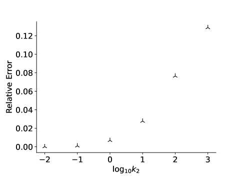
Figure 3: The relative error between the QSS variance of GSPT-derived ssLNA and QSS variance of the LNA for $p$ decreases as $k_{2},k_{3}\to 0$. The $y$-axis is the relative error $|\Sigma(1,1)-\sigma_{p}|/\Sigma(1,1)$; the $x$-axis is $\log_{10}k_{2}$. Parameters (in arbitrary units) are: $e_{T}=1000.0$, $s_{T}=2000.0$, $k_{1}=1.0$, $k_{-1}=1.0$ and $\Omega=1.0$ The parameters $k_{2}$ and $k_{3}$ are equal range and from $10^{3}$ to $10^{-2}$.

5 Reduction of the CME: Intimations from the linear noise regime

In this section, we discuss the reduction of the CME for the MM reaction mechanism and its relationship to singular perturbations and critical manifolds. Specifically, we address the presence of transcritical bifurcations in the linear noise regime and illustrate that knowledge of the critical manifold can assist in avoiding erroneous conclusions concerning the validity of the stochastic QSSA.

5.1 Dynamic bifurcations and the Segel–Slemrod sQSS condition

The CME for the MM reaction mechanism is

$$\cfrac{\partial}{\partial t}P(n_{S},n_{C},t)=\bigg{[}\cfrac{k_{1}}{\Omega}(\mathbb{E}_{S}^{+1}\mathbb{E}_{C}^{-1}n_{S}(n_{e_{T}}-n_{C})\\ +k_{-1}(\mathbb{E}_{S}^{+1}\mathbb{E}_{C}^{-1}-1)n_{C}+k_{2}(\mathbb{E}_{C}^{-1}-1)n_{C}\bigg{]}P(n_{S},n_{C},t).$$ (72)

where $n_{e_{T}}$ denotes the total number of enzyme molecules, and $P(n_{S},n_{C},t)$ is the probability of finding the system with $n_{S}$ substrate molecules and $n_{C}$ complex molecules at time $t$.

The homologous sQSS reduction of (72) is as follows. Given that there are $n_{S}$ substrate molecules at time $t$, the probability that one one product molecule forms in an infinitesimal window $[t,t+\text{d}t)$ is

$$P(n_{S}-1,t+\text{d}t|n_{S},t):=a(n_{S})\text{d}t=\cfrac{k_{2}e_{T}n_{S}}{K_{M}+n_{S}/\Omega}\;\text{d}t,$$ (73)

where the propensity function, $a(n_{S})$, is adopted from deterministic sQSSA rate law, and the reduced CME is

$$\cfrac{\partial}{\partial t}P(n_{S},t)=(\mathbb{E}_{S}^{+1}-1)\cfrac{k_{2}e_{T}n_{S}}{K_{M}+n_{S}/\Omega}P(n_{S},t).$$ (74)

In what follows, for simplicity, we set $\Omega=1$ and work in arbitrary units; however, we perform our simulations with a large number of molecules.

Numerical work by Sanft et al. [31] suggests that the Segel–Slemrod condition (expressed in terms of stochastic rate constants)

$$e_{T}\ll K_{M}+s_{T}$$ (75)

ensures the validity of the stochastic sQSSA (74). This is surprising, especially since the long-time validity of the deterministic sQSSA for the MM reaction mechanism requires $e_{T}/K_{M}\ll 1$ [5], which is more restrictive than the Segel and Slemrod condition. However, excellent (and extremely rigorous) work by Kang et al. [32] disputes this claim. In the stochastic regime, Kang et al. [32] concluded that $e_{T}\ll K_{M}$, which is in agreement with the deterministic qualifier. A similar conclusion was drawn by Mastny et al. [33].

Importantly, although the deterministic and stochastic QSS reductions of the MM mechanism are justified via singular perturbation theory, the rigorous derivation of the sQSSA from singular perturbation was only recently established Goeke et al. [10]. This raises the question: given what we now understand about the bifurcation structure of the critical set associated with the deterministic MM reaction mechanism, what consequence(s) does this have on the stochastic QSS reduction? More specifically, does the Segel and Slemrod condition guarantee that the stochastic sQSSA will remain accurate for all time, or is the more restrictive condition derived by Kang et al. [32] and Mastny et al. [33] necessary to ensure the accuracy of the stochastic sQSSA?

To answer this question, we note that the perturbation problem corresponding to small $k_{-1}$ and $k_{2}$ is of the form (48):

$$\dot{p} =\varepsilon\widehat{k}_{2}c$$ (76a)

$$\dot{c} =k_{1}(e_{T}-c)(s_{T}-c-p)-\varepsilon(\widehat{k}_{-1}+\widehat{k}_{2}).$$ (76b)

If $e_{T}\ll s_{T}=s(0)$, then the Fenichel reduction is formulated by projecting the perturbation onto the tangent space of $\mathcal{S}_{a}^{r}$, $T_{z}\mathcal{S}_{a}^{r}$:

$$\dot{p} =k_{2}e_{T},$$ (77a)

$$\dot{c} =0.$$ (77b)

This approximation does not hold for all-time: eventually the trajectory follows $\mathcal{S}_{a}^{b}$, and the Fenichel reduction is

$$\dot{p} =k_{2}(s_{T}-p),$$ (78a)

$$\dot{c} =-k_{2}(s_{T}-p).$$ (78b)

The behavior of the reduction in small neighborhoods containing the bifurcation point is beyond the scope of this paper. In general, one must defer to non-classical methods to derive scaling laws near the bifurcation point (see, Berglund and Gentz [34], Krupa and Szmolyan [35]).

As $\Omega$ shrinks and fluctuations emerge, the LNA holds sway. The presence of a bifurcation point in the critical set is not too restrictive in this case. The ssLNA obtained via projection onto $\mathcal{S}_{a}^{r}$ is

$$\dot{p} =k_{2}e_{T},$$ (79a)

$$\text{d}X_{p} =\Omega^{-1/2}\sqrt{k_{2}e_{T}}\;\text{d}W_{3}.$$ (79b)

Note the relationship between the mean and variance. Likewise, projecting onto $T_{z}\mathcal{S}_{a}^{b}$ yields

$$\dot{p} =k_{2}(s_{T}-p),$$ (80a)

$$\text{d}X_{p} =-k_{2}X_{p}\text{d}t+\Omega^{-1/2}\sqrt{k_{2}(s_{T}-p)}\;\text{d}W_{3}.$$ (80b)

As $\Omega\to 0$ the CME prevails as the physically relevant model. The ssLNA (79) is a Gaussian process with equal mean and variance. In the CME regime, the reaction mechanism on $\mathcal{S}_{a}^{r}$ is equivalent to

$$\emptyset\ce{->[$\lambda$]P},$$ (81)

where $\lambda=k_{2}n_{e_{T}}$ and $n_{e_{T}}$ denotes the total number (bound or unbound) of enzyme molecules. The CME that describes (81) is solvable. Let $P(N,t)$ denote the probability that there are $N$ product molecules at time $t$. Then,

$$P(N,t)=\exp{(-\lambda t)}\cdot\cfrac{(\lambda t)^{N}}{N!}.$$ (82)

Note the consistency with (79). The Poisson jump process is approximately Gaussian when the system size is sufficiently large.

Unfortunately, (82) is not valid for all-time, and it is necessary to ascertain the range of its validity. More precisely, we ask: How long (on average) from the onset of the reaction does it take before (84) is valid? Since (81) is a Poisson process the jump times, $t_{N}$, are gamma-distributed:

$$t_{N}\sim\lambda^{N}\exp{(-\lambda t)}\cdot\cfrac{t^{N-1}}{(N-1)!}.$$

Let $n_{s_{T}}$ denote the total number of substrate molecules. The average time it takes to produce $N^{*}=n_{S_{T}}-n_{e_{T}}$ product molecules is

$$\langle t_{N^{*}}\rangle=\cfrac{N^{*}}{\lambda},$$

which is exactly homologous to the deterministic scenario.

Moving on, once $N=n_{S_{T}}-n_{e_{T}}$ we arrive at the intersection of the critical branches, $\mathcal{S}_{a}^{r}\cap\mathcal{S}_{a}^{b}$. At this point, no substrate molecules remain and the formation product is synonymous with the depletion of $c$:

$$C\ce{->[$k_{2}$]P}.$$ (83)

Once again, the CME associated with (83) is solvable:

$$P(n_{S_{T}}-n_{c},t)=P(n_{c},t)=\exp(-k_{2}n_{c}t)\begin{pmatrix}n_{e_{T}}\\ n_{c}\end{pmatrix}(1-\exp(-k_{2}t))^{(n_{e_{T}}-n_{c})},$$ (84)

where $n_{c}$ denotes the number of complex molecules, and time has been translated so that:

$$P(n_{S_{T}}-n_{e_{T}},0)=1.$$

The question that remains is: How should the Gillespie algorithm be modified to reduce the computational complexity when $k_{2}$ and $k_{-1}$ are sufficiently small? The above analysis indicates that $P(N,t)$ depends on the number of product molecules present at a given time in the reaction. Specifically, $P(N,t)$ depends on whether or not $N<N^{*}$. To modify the Gillespie algorithm, observe that the propensity function $a(N)$ for product formation – at any given time – depends on the number of product molecules, $N$, present at time $t$. Thus,

$$a(N)=\begin{cases}k_{2}n_{e_{T}},\qquad\text{if}\;\;N<N^{*},\\ k_{2}n_{c},\qquad\;\;\text{if}\;\;N\geq N^{*}.\end{cases}$$ (85)

Numerical simulations support the results of our analysis, and demonstrate that the Segel and Slemrod condition does not imply the validity of the stochastic sQSSA (see Figure 4).

We note that one can employ the reduction technique of Thomas et al. [14]. In general, the ssLNA of Thomas et al. [14] will be close (in the asymptotic sense) to (79)–(80), but will be more complicated due to the presence of additional diffusion terms. The simplicity of the GSPT-derived ssLNA (79)–(80) helps to explain the insufficiency of the Segel–Slemrod condition for the validity of the stochastic sQSSA in the linear noise regime, thereby validating the results of Kang et al. [32] and Mastny et al. [33] from the context of GSPT.

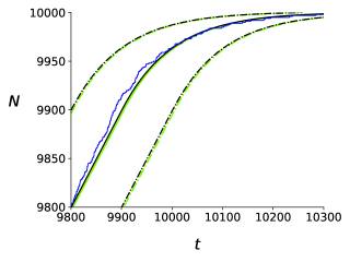
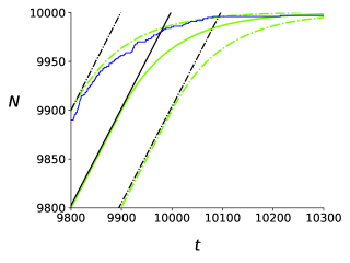
Figure 4: The stochastic sQSSA (73) will fail near the bifurcation point if $e_{T}/K_{M}\gg 1$. In both panels, the solid green curve is the numerically-computed mean of the timecourse for $N$ (the number of product molecules) obtained from $1000$ simulations generated by the Gillespie algorithm; the dashed/dotted green curves demarcate the mean $\pm$ the standard deviation. The solid black curve is the numerically-computed mean of the time course for $N$ (the number of product molecules) obtained from $1000$ simulations generated by the Gillespie algorithm equipped with a QSS-derived propensity function; the blue line shows one such randomly picked simulation; the dashed/dotted black lines demarcate the mean $\pm$ the standard deviation. In both simulations, the parameters (in arbitrary units) are: $n_{s_{T}}=10000$, $n_{e_{T}}=100$, $k_{1}=1000.0$, $k_{-1}=0.01$, $k_{2}=0.01$ and $\Omega=1.0$. $n_{s}(0)=n_{s_{T}}$, $n_{c}(0)=0$, $n_{e}(0)=n_{e_{T}}$, and $N(0)=0$. Note that $e_{T}/(K_{M}+s_{T})\approx 0.01$ and therefore the Segel-Slemrod (75) condition holds. Left panel: The black solid and dashed/dotted lines are obtained from Gillespie algorithm equipped with the propensity function (85); the first two statistical moments are practically indistinguishable. Right panel: The black solid and dashed/dotted lines are obtained from Gillespie algorithm equipped with the propensity function (73), and the stochastic sQSSA fails near $N=N^{*}$.

As a final remark, we mention that the bifurcation point can also be handled with appropriate utilization of the tQSSA. Although the treatment of bifurcation points has so far not been addressed in the stochastic tQSSA literature, several rigorous studies suggest that the stochastic tQSSA is superior to the sQSSA in the CME and LNA regimes. Rigorous analyses of the stochastic tQSSA are found in [36, 37, 38, 39, 40].

6 Discussion

The primary contribution of this work is the derivation of the ssLNA in a way that is consistent with Fenichel theory [3], that is, the projection of a perturbation term onto the tangent space of a normally hyperbolic critical manifold. Our derivation explains the origin of the differences between the the ssLNAs reported in Thomas et al. [14], Pahlajani et al. [15], and Herath and Del Vecchio [16].

By re-deriving the ssLNA directly from GSPT, we illustrated how the GSPT-derived ssLNA can be extended to singular perturbation problems where normal hyperbolicity fails and classical Fenichel theory breaks down. To the best of our knowledge, this is the first extension of the ssLNA to singular perturbation problems that contain a transcritical bifurcation.

Finally, let us remark on the possible special role of the standard form in the reduction of the CME. In their derivation of the ssLNA, Thomas et al. [14] shared the following insight: the mapping

$$\mathcal{S}_{slow}\mapsto\mathcal{S}_{slow}-\cfrac{f_{y}}{g_{y}}\cdot\mathcal{S}_{fast}$$

does not result in physically meaningful slow variable stoichiometry in the CME regime. However, as we pointed out, when the system is truly in standard form (again, the MM reaction mechanism with small $e_{T}$ does not technically qualify), the stoichiometry component of the slow variable, $\mathcal{S}_{slow}$ is invariant: $\mathcal{S}_{slow}\mapsto\mathcal{S}_{slow}$. This suggests that singularly perturbed systems in standard form might, in some way, be amenable to QSS reduction in the CME regime. However, this hypothesis warrants further investigation.

References

- Tikhonov [1952] A. Tikhonov, Systems of differential equations containing small parameters in their derivatives, Mat. Sb. (N.S.) 31 (1952) 575–586.
- Fenichel [7172] N. Fenichel, Persistence and smoothness of invariant manifolds for flows, Indiana Univ. Math. J. 21 (1971/72) 193–226.
- Fenichel [1979] N. Fenichel, Geometric singular perturbation theory for ordinary differential equations, J. Differ. Equations 31 (1979) 53–98.
- Eilertsen et al. [2019] J. Eilertsen, W. Stroberg, S. Schnell, Characteristic, completion or matching timescales? an analysis of temporary boundaries in enzyme kinetics, J. Theor. Biol. 481 (2019) 28–43.
- Eilertsen and Schnell [2020] J. Eilertsen, S. Schnell, The quasi-steady-state approximations revisited: Timescales, small parameters, singularities, and normal forms in enzyme kinetics, Math. Biosci. 325 (2020) 108339.
- Goeke et al. [2017] A. Goeke, S. Walcher, E. Zerz, Classical quasi-steady state reduction – A mathematical characterization, Physica D 345 (2017) 11–26.
- Goeke et al. [2015] A. Goeke, S. Walcher, E. Zerz, Determining “small parameters” for quasi-steady state, J. Differ. Equations. 259 (2015) 1149–1180.
- Noethen and Walcher [2011] L. Noethen, S. Walcher, Tikhonov’s theorem and quasi-steady state, Discrete Contin. Dyn. Syst. Ser. B 16 (2011) 945–961.
- Eilertsen et al. [2021] J. Eilertsen, M. Roussel, S. Schnell, S. Walcher, On the quasi-steady-state approximation in an open Michaelis–Menten reaction mechanism, AIMS Math 6 (2021) 6781––6814.
- Goeke et al. [2012] A. Goeke, C. Schilli, S. Walcher, E. Zerz, Computing quasi-steady state reductions, J. Math. Chem. 50 (2012) 1495–1513.
- Kan et al. [2016] X. Kan, C. H. Lee, H. G. Othmer, A multi-time-scale analysis of chemical reaction networks: II. Stochastic systems, J. Math. Biol. 73 (2016) 1081–1129.
- Kim et al. [2017] J. K. Kim, G. A. Rempala, H.-W. Kang, Reduction for stochastic biochemical reaction networks with multiscale conservations, Multiscale. Model. Simul. 15 (2017) 1376–1403.
- Kang and Kurtz [2013] H.-W. Kang, T. G. Kurtz, Separation of time-scales and model reduction for stochastic reaction networks, Ann. Appl. Probab. 23 (2013) 529–583.
- Thomas et al. [2012] P. Thomas, A. V. Straube, R. Grima, The slow-scale linear noise approximation: an accurate, reduced stochastic description of biochemical networks under timescale separation conditions, BMC Sys. Biol. 6 (2012) 39.
- Pahlajani et al. [2011] C. D. Pahlajani, P. J. Atzberger, M. Khammash, Stochastic reduction method for biological chemical kinetics using time-scale separation, J. Theo. Biol. 272 (2011) 96–112.
- Herath and Del Vecchio [2018] N. Herath, D. Del Vecchio, Reduced linear noise approximation for biochemical reaction networks with time-scale separation: The stochastic tQSSA+, J. Chem. Phys. 148 (2018) 094108.
- Wechselberger [2020] M. Wechselberger, Geometric Singular Perturbation Theory Beyond the Standard Forms, number 6 in Frontiers in Applied dynamical systems: Tutorials and Reviews, Springer, 2020.
- Goeke and Walcher [2014] A. Goeke, S. Walcher, A constructive approach to quasi-steady state reductions, J. Math. Chem. 52 (2014) 2596–2626.
- Goeke [2013] A. Goeke, Reduktion und asymptotische reduktion von reaktionsgleichungen, Doctoral Dissertation, RWTH Aachen (2013).
- Goeke et al. [2015] A. Goeke, S. Walcher, E. Zerz, Determining “small parameters” for quasi-steady state, J. Differential Equations 259 (2015) 1149–1180.
- Heineken et al. [1967] F. G. Heineken, H. M. Tsuchiya, R. Aris, On the mathematical status of the pseudo-steady hypothesis of biochemical kinetics, Math. Biosci. 1 (1967) 95–113.
- Segel and Slemrod [1989] L. A. Segel, M. Slemrod, The quasi-steady-state assumption: A case study in perturbation, SIAM Rev. 31 (1989) 446–477.
- Segel [1988] L. A. Segel, On the validity of the steady state assumption of enzyme kinetics, Bull. Math. Biol. 50 (1988) 579–593.
- Schnell and Maini [2000] S. Schnell, P. K. Maini, Enzyme kinetics at high enzyme concentration, Bull. Math. Biol. 62 (2000) 483–499.
- Gillespie [1992] D. T. Gillespie, A rigorous derivation of the chemical master equation, Physica A 188 (1992) 404–425.
- Kampen [2007] N. V. Kampen, Chapter V. The Master Equation, in: Stochastic Processes in Physics and Chemistry ( Edition), North-Holland Personal Library, Elsevier, Amsterdam, 2007, pp. 96–133.
- Thomas et al. [2012] P. Thomas, R. Grima, A. V. Straube, Rigorous elimination of fast stochastic variables from the linear noise approximation using projection operators, Phys. Rev. E 86 (2012) 041110.
- Katzenberger [1991] G. S. Katzenberger, Solutions of a stochastic differential equation forced onto a manifold by a large drift, Ann. Probab. 19 (1991) 1587–1628.
- Parsons and Rogers [2017] T. L. Parsons, T. Rogers, Dimension reduction for stochastic dynamical systems forced onto a manifold by large drift: a constructive approach with examples from theoretical biology, J. Phys. A Math. Theor. 50 (2017) 415601.
- Thomas et al. [2011] P. Thomas, A. V. Straube, R. Grima, Communication: Limitations of the stochastic quasi-steady-state approximation in open biochemical reaction networks, J. Chem. Phys. 135 (2011) 181103.
- Sanft et al. [2011] K. Sanft, D. T. Gillespie, L. R. Petzold, The legitimacy of the stochastic Michaelis–Menten approximation, IET Syst. Biol. 5 (2011) 58–69.
- Kang et al. [2019] H.-W. Kang, W. R. KhudaBukhsh, H. Koeppl, G. Rempala, Quasi-steady-state approximations derived from the stochastic model of enzyme kinetics, Bull. Math. Biol. 81 (2019) 1303–1336.
- Mastny et al. [2007] E. A. Mastny, E. L. Haseltine, J. B. Rawlings, Two classes of quasi-steady-state model reductions for stochastic kinetics, J. Chem. Phys. 127 (2007) 094106.
- Berglund and Gentz [2006] N. Berglund, B. Gentz, Noise-induced phenomena in slow-fast dynamical systems, Springer-Verlag London, Ltd., London, 2006.
- Krupa and Szmolyan [2001] M. Krupa, P. Szmolyan, Extending slow manifolds near transcritical and pitchfork singularities, Nonlinearity 14 (2001) 1473–1491.
- Kim et al. [2014] J. Kim, K. Josić, M. Bennett, The validity of quasi-steady-state approximations in discrete stochastic simulations, Biophys. J. 107 (2014) 783 – 793.
- Kim and Tyson [2020] J. K. Kim, J. J. Tyson, Misuse of the michaelis–-menten rate law for protein interaction networks and its remedy, PLoS Comp. Biol. 16 (2020) 1–21.
- Kim et al. [2015] J. K. Kim, K. Josić, M. R. Bennett, The relationship between stochastic and deterministic quasi-steady state approximations, BMC Syst. Biol. 9 (2015) 87.
- MacNamara et al. [2008] S. MacNamara, A. M. Bersani, K. Burrage, R. B. Sidje, Stochastic chemical kinetics and the total quasi-steady-state assumption: Application to the stochastic simulation algorithm and chemical master equation, J. Chem. Phys. 129 (2008) 095105.
- Barik et al. [2008] D. Barik, M. R. Paul, W. T. Baumann, Y. Cao, J. J. Tyson, Stochastic simulation of enzyme-catalyzed reactions with disparate timescales, Biophys. J. 95 (2008).