Is NOMA Efficient in Multi-Antenna Networks?
A Critical Look at Next Generation Multiple Access Techniques

Abstract

In the past few years, a large body of literature has been created on downlink Non-Orthogonal Multiple Access (NOMA), employing superposition coding and Successive Interference Cancellation (SIC), in multi-antenna wireless networks. Furthermore, the benefits of NOMA over Orthogonal Multiple Access (OMA) have been highlighted. In this paper, we take a critical and fresh look at this downlink multiple access literature. Instead of contrasting NOMA with OMA, we contrast NOMA with two other baselines. The first is conventional Multi-User Linear Precoding (MU–LP), as used in Space-Division Multiple Access (SDMA) and multi-user Multiple-Input Multiple-Output (MIMO) in 4G and 5G. The second is Rate-Splitting Multiple Access (RSMA) based on multi-antenna Rate-Splitting (RS), which is also a non-orthogonal transmission strategy relying on SIC developed in the past few years in parallel and independently from NOMA. We show that there is some confusion about the benefits of NOMA, and we dispel the associated misconceptions. First, we highlight why NOMA is inefficient in multi-antenna settings (compared to the baselines) based on basic multiplexing gain analysis. We stress that the issue lies in how the NOMA literature, originally developed for single-antenna setups, has been hastily applied to multi-antenna setups, resulting in a misuse of spatial dimensions and therefore loss in multiplexing gains and rate. Second, we show that NOMA incurs a severe multiplexing gain loss despite an increased receiver complexity due to an inefficient use of SIC receivers. Third, we emphasize that much of the merits of NOMA are due to the constant comparison to OMA instead of comparing it to MU–LP and RS baselines. We then expose the pivotal design constraint that multi-antenna NOMA requires one user to fully decode the messages of the other users. This design constraint is responsible for the multiplexing gain erosion, rate loss, and inefficient use of SIC receivers in multi-antenna settings. Our analysis and simulations confirm that NOMA should not be applied blindly to multi-antennas settings, highlight the scenarios where MU–LP outperforms NOMA and vice versa, and demonstrate the inefficiency, performance loss and complexity disadvantages of NOMA compared to RS. The first takeaway message is that, while NOMA is suited for single-antenna settings (as originally intended), it is not beneficial in most multi-antenna deployments. The second takeaway message is that other non-orthogonal transmission frameworks, such as RS, exist which fully exploit the multiplexing gain and the benefits of SIC to boost the rate in multi-antenna settings.

I Introduction

In contrast to Orthogonal Multiple Access (OMA) that assigns users to orthogonal dimensions (e.g., Time-Division Multiple Access - TDMA, Frequency-Division Multiple Access - FDMA), (power-domain) Non-Orthogonal Multiple Access (NOMA) superposes users in the same time-frequency resource and distinguishes them in the power domain [1, 2, 3, 4, 5]. By doing so, NOMA has been promoted as a solution for 5G and beyond to deal with the vast throughput, access, and quality of service (QoS) requirements that are projected to grow exponentially for the foreseeable future.

In the downlink, NOMA refers to communication schemes where at least one user is forced to fully decode the message(s) of other co-scheduled user(s). This operation is commonly performed through the use of transmit-side superposition coding (SC) and receiver-side Successive Interference Cancellation (SIC) in downlink multi-user communications. Such techniques have been studied for years before being branded with the NOMA terminology. NOMA has indeed been known in the information theory and wireless communications literature for several decades, under the terminology of superposition coding with successive interference cancellation (denoted in short as SC–SIC), as the strategy that achieves (and has been used in achievability proofs for) the capacity region of the Single-Input Single-Output (SISO) (Gaussian) Broadcast Channel (BC) [6]. The superiority of NOMA over OMA was shown in the seminal paper by Cover in 1972. It is indeed well known that the capacity region of the SISO BC (achieved by NOMA) is larger than the rate region achieved by OMA (i.e. contains the achievable rate region of OMA as a subset) [6, 7, 8]. The use of SIC receivers is a major difference between NOMA and OMA, although it should be mentioned that SIC has also been studied for a long time in the 3G and 4G research phases in the context of interference cancellation and receiver designs [9].

In today’s wireless networks, access points commonly employ more than one antenna, which opens the door to multi-antenna processing. The key building block of the downlink of multi-antenna networks is the multi-antenna (Gaussian) BC. Contrary to the SISO BC that is degraded and where users can be ordered based on their channel strengths, the multi-antenna BC is nondegraded and users cannot be ordered based on their channel strengths [10, 7]. This is the reason why SC–SIC/NOMA is not capacity-achieving in this case, and Dirty Paper Coding (DPC) is the only known strategy that achieves the capacity region of the multi-antenna (Gaussian) BC with perfect Channel State Information at the Transmitter (CSIT) [10]. Due to the high computational burden of DPC, linear precoding is often considered the most attractive alternative to simplify the transmitter design [11, 12, 13, 14, 15]. Interestingly, in a multi-antenna BC, Multi-User Linear Precoding (MU–LP) relying on treating the residual multi-user interference as noise, although suboptimal, is often very useful since the interference can be significantly reduced by spatial precoding. This is the reason why it has received significant attention in the past twenty years and it is the basic principle behind numerous 4G and 5G techniques such as Space-Division Multiple Access (SDMA) and multi-user (potentially massive) Multiple-Input Multiple-Output (MIMO) [15].

In view of the benefits of NOMA over OMA and multi-antenna over single-antenna, numerous attempts have been made in recent years to combine multi-antenna and NOMA schemes [1, 2, 3, 4, 5, 16, 17, 18, 19, 20, 21, 22, 38, 39, 23, 24, 25, 26, 27, 28, 29, 30, 31, 32, 33, 34, 35, 36, 37] (and references therein). Although there are a few contributions considering the comparison of NOMA with MU–LP schemes such as Zero-Forcing Beamforming (ZFBF) or DPC [38, 39, 26, 40], much emphasis is put in the NOMA literature on comparing (single/multi-antenna) NOMA and OMA, and showing that NOMA outperforms OMA. But there is a lack of emphasis in the NOMA literature on contrasting multi-antenna NOMA to other multi-user multi-antenna baselines developed for the multi-antenna BC such as MU–LP (or other forms of multi-user MIMO techniques) and other forms of (power-domain) non-orthogonal transmission strategies such as Rate-Splitting Multiple Access (RSMA) based on multi-antenna Rate-Splitting (RS) [41]. RS designed for the multi-antenna BC also relies on SIC and has been developed in parallel and independently from NOMA [41, 42, 43, 44, 45, 46, 47]. Such a comparison is essential to assess the benefits and the efficiency of NOMA, since all these communication strategies can be viewed as different achievable schemes for the multi-antenna BC and all aim in their own way for the same objective, namely meet the throughput, reliability, QoS, and connectivity requirements of beyond-5G multi-antenna wireless networks.

In this paper, we take a critical look at multi-antenna NOMA for the downlink of communication systems and ask ourselves the important question “Is multi-antenna NOMA an efficient strategy?” To answer this question, we go beyond the conventional NOMA vs. OMA comparison, and contrast multi-antenna NOMA with MU–LP and RS-based non-orthogonal transmission strategies. This allows us to highlight some misconceptions and shortcomings of multi-antenna NOMA. Explicitly, we show that in most scenarios the short answer to that question is no, and demonstrate based on first principles and numerical performance evaluations why this is the case. Our discussions and results unveil the scenarios where MU–LP outperforms NOMA and vice versa, and demonstrate that multi-antenna NOMA is inefficient compared to RS.

By contrasting multi-antenna NOMA to MU–LP and RS, we show that there is some confusion about multi-antenna NOMA and its merits, expose major misconceptions and reveal new insights. The contributions of this paper are summarized as follows.

First, we analytically derive both the sum multiplexing gain as well as the max-min fair multiplexing gain of multi-antenna NOMA and compare them to those of MU–LP and RS. The scenarios considered are very general and include multi-antenna transmitter with single-antenna receivers, perfect and imperfect CSIT, in underloaded and overloaded regimes. On the one hand, multi-antenna NOMA can achieve gains, but can also incur losses compared to MU–LP. On the other hand, multi-antenna NOMA always leads to a waste of multiplexing gain compared to RS. The multiplexing gain analysis provides a firm theoretical ground to infer that multi-antenna NOMA is not as efficient as RS in exploiting the spatial dimensions and the available CSIT. This analysis is instrumental to identify the scenarios where the multiplexing gain gaps among NOMA, MU–LP, and RS are the smallest/largest, therefore highlighting deployments that are suitable/unsuitable for the different multiple access strategies.

Second, we show that multi-antenna NOMA leads to a high receiver complexity due to the inefficient use of SIC. For instance, we show that the higher the number of SIC operations (and therefore the higher the receiver complexity) in multi-antenna NOMA, the lower the sum multiplexing gain (and therefore the lower the sum-rate at high SNR). Comparison with MU–LP and RS show that higher multiplexing gains can be achieved at a lower receiver complexity and a reduced number of SIC operations.

TABLE I: Overview of the paper.

Section II. Two-User MISO NOMA with Perfect CSIT: The Basic Building Block
II-A. System Model	II-B. Definition of Multiplexing Gain
II-C. Discussions
Section III. $K$-User MISO NOMA with Perfect CSIT
III-A. MISO NOMA System Model	III-B. Multiplexing Gains
Section IV. $K$-User MISO NOMA with Imperfect CSIT
IV-A. CSIT Error Model	IV-B. Multiplexing Gains
Section V. Baseline Scheme I: Conventional Multi-user Linear Precoding
V-A. MU–LP System Model	V-B. Multiplexing Gains with Perfect CSIT
V-C. Multiplexing Gains with Imperfect CSIT
Section VI. Baseline Scheme II: Rate-Splitting
VI-A. Rate-Splitting System Model	VI-B. Multiplexing Gains with Perfect CSIT
VI-C. Multiplexing Gains with Imperfect CSIT
Section VII. Shortcomings and Misconceptions of Multi-Antenna NOMA
VII-A. NOMA vs. Baseline I (MU–LP)	VII-B. NOMA vs. Baseline II (RS)
VII-C. Misconceptions of Multi-Antenna NOMA	VII-D. Illustration of the Misconceptions with an Example
VII-E. Shortcomings of Multi-Antenna NOMA
Section VIII. Numerical Results
VIII-A. Perfect CSIT	VIII-B. Imperfect CSIT
VIII-C. Discussions
Section IX. Conclusions and Future Works

Third, we show that most of the misconceptions behind NOMA are due to the prevalent comparison to OMA instead of comparing to MU–LP and RS. We show and explain that the misconceptions, the multiplexing gain reduction, and the inefficient use of SIC receivers in both underloaded and overloaded multi-antenna settings reyling on both perfect and imperfect CSIT originate from a limitation of the multi-antenna NOMA design philosophy, namely that one user is forced to fully decode the messages of the other users. Hence, while forcing a user to fully decode the messages of the other users is an efficient approach in single-antenna degraded BC, it may not be an efficient approach in multi-antenna networks.

Fourth, we stress that an efficient design of non-orthogonal transmission and multiple access strategies ensures that the use of SIC never leads to a performance loss but rather leads to a performance gain over MU–LP. We show that such non-orthogonal solutions based on RS exist and truly benefit from the multi-antenna multiplexing gain and from the use of SIC receivers in both underloaded and overloaded regimes relying on perfect and imperfect CSIT. In fact, multi-antenna RS completely resolves the design limitations of multi-antenna NOMA.

Fifth, we depart from the multiplexing gain analysis and design the transmit precoders to maximize the sum-rate and max-min rate for multi-antenna NOMA, followed by numerically comparing the sum-rate and the max-min fair rate of NOMA to those of MU–LP and RS. We show that the multiplexing gain analysis is accurate and instrumental to predict the rate performance of the multiple access strategies considered.

Sixth, our numerical simulations confirm the inefficiency of multi-antenna NOMA in general settings. Multi-antenna NOMA is shown to lead to performance gains over MU–LP in some settings but also to losses in other settings despite the use of SIC receivers and a higher receiver complexity. Our results also highlight the significant benefits, performance-wise and receiver complexity-wise, of RSMA and multi-antenna RS over multi-antenna NOMA. It is indeed possible to achieve a significantly better performance than MU–LP and NOMA with just one layer of SIC by adopting RS so as to partially decode messages of other users (instead of fully decoding them as in NOMA).

Organization: The remainder of this paper is organized as follows. Section II introduces two-user Multiple-Input Single-Output (MISO) NOMA (with single-antenna receivers) as a basic building block (and toy example) for our subsequent studies, compares to MU–LP, and raises some questions about the efficiency of NOMA. Section III studies the multiplexing gain of $K$-user MISO NOMA with perfect CSIT. Section IV extends the discussion to imperfect CSIT. Section V and Section VI study the multiplexing gains of the baseline schemes considered, namely MU–LP and RS, respectively. Section VII compares the multiplexing gains of all multiple access schemes considered and exposes the misconceptions and shortcomings of multi-antenna NOMA. Section VIII provides simulation results. Section IX concludes this paper. An overview of the paper is illustrated in Table I.

Notation: $|\cdot|$ refers to the absolute value of a scalar or to the cardinality of a set depending on the context. $\left\|\cdot\right\|$ refers to the $l_{2}$-norm of a vector. $\max\{a_{1},...,a_{n}\}$ refers to the maximum value between $a_{1}$ to $a_{n}$. $\mathbf{a}^{H}$ denotes the Hermitian transpose of vector $\mathbf{a}$. $\textrm{Tr}(\mathbf{Q})$ refers to the trace of matrix $\mathbf{Q}$. $\mathbf{I}$ is the identity matrix. $P\nearrow$ means as $P$ grows large. $\mathcal{CN}(0,\sigma^{2})$ denotes the circularly symmetric complex Gaussian distribution with zero mean and variance $\sigma^{2}$. $\sim$ stands for “distributed as”. $O(\cdot)$ refers to the big O notation. $\mathbb{E}\big{\{}\cdot\big{\}}$ denotes statistical expectation. $A\cap B$ and $A\cup B$ refer to the intersection ($A$ and $B$ have to be satisfied) and the union ($A$ or $B$ to be satisfied) of two sets/events $A$ and $B$, respectively.

II Two-User MISO NOMA with Perfect CSIT:
The Basic Building Block

We commence by studying two-user MISO NOMA and show that, by comparing NOMA to MU–LP instead of to OMA, the potential merits of NOMA are less obvious. Limited to two single-antenna users with perfect CSIT, this system model illustrates the simplest though fundamental building block of multi-antenna NOMA.

II-A System Model

We consider a downlink single-cell multi-user multi-antenna scenario with $K=2$ users, also known as two-user MISO BC, consisting of one transmitter with $M\geq 2$ antennas communicating with two single-antenna users. The transmitter aims to transmit simultaneously two messages $W_{1}$ and $W_{2}$ intended for user-1 and user-2, respectively.

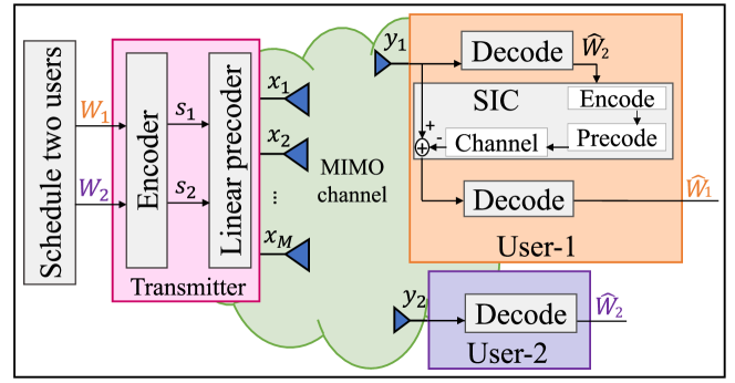
Figure 1: Two-user system architecture with NOMA (decoding order: user-2$\rightarrow$user-1).

The transmitter adopts the so-called multi-antenna NOMA or MISO NOMA strategy, illustrated in Fig. 1, that encodes one of the two messages using a codebook shared by both users so that it can be decoded and cancelled from the received signal at the co-scheduled user (following the same principle as superposition coding for the degraded BC). Consider $W_{2}$ is encoded into $s_{2}$ using the shared codebook and $W_{1}$ is encoded into $s_{1}$. The two streams are then linearly precoded by $M\times 1$ precoders $\mathbf{p}_{1}$ and $\mathbf{p}_{2}$ and superposed at the transmitter so that the transmit signal is given by

$$\mathbf{x}=\mathbf{p}_{1}s_{1}+\mathbf{p}_{2}s_{2}.$$ (1)

Defining $\mathbf{s}=[s_{1},s_{2}]^{T}$ and assuming that $\mathbb{E}[\mathbf{s}\mathbf{s}^{H}]=\mathbf{I}$, the average transmit (sum) power constraint is written as $P_{1}+P_{2}\leq P$ where $P_{k}=\left\|\mathbf{p}_{k}\right\|^{2}$ with $k=1,2$.

The channel vector for user $k$ is denoted by $\mathbf{h}_{k}$, and the received signal at user $k$ can be written as $y_{k}=\mathbf{h}_{k}^{H}\mathbf{x}+n_{k}$, $k=1,2$, where $n_{k}\sim\mathcal{CN}(0,1)$ is Additive White Gaussian Noise (AWGN). We assume perfect CSIT and perfect Channel State Information at the Receivers (CSIR).

At both users, stream $s_{2}$ is decoded first into $\widehat{W}_{2}$ by treating the interference from $s_{1}$ as noise. Using SIC at user-1, $\widehat{W}_{2}$ is re-encoded, precoded, and subtracted from the received signal, such that user-$1$ can decode its stream $s_{1}$ into $\widehat{W}_{1}$. Assuming proper Gaussian signalling and perfect SIC, the achievable rates of the two streams with MISO NOMA are given by

$$R_{1}^{(\textnormal{N})} =\log_{2}\left(1+\left|\mathbf{h}_{1}^{H}\mathbf{p}_{1}\right|^{2}\right),$$ (2)

$$R_{2}^{(\textnormal{N})} =\min\left(\log_{2}\left(1+A\right),\log_{2}\left(1+B\right)\right),$$ (3)

where

$$A=\frac{\left|\mathbf{h}_{1}^{H}\mathbf{p}_{2}\right|^{2}}{1+\left|\mathbf{h}_{1}^{H}\mathbf{p}_{1}\right|^{2}},\hskip 28.45274ptB=\frac{\left|\mathbf{h}_{2}^{H}\mathbf{p}_{2}\right|^{2}}{1+\left|\mathbf{h}_{2}^{H}\mathbf{p}_{1}\right|^{2}}.$$ (4)

In (3), $\log_{2}\left(1+A\right)$ is the rate supportable by the channel of user-1 when user-1 decodes $s_{2}$ and treats its own stream $s_{1}$ as noise. Similarly, $\log_{2}\left(1+B\right)$ is the rate supportable by the channel of user-2 when user-2 decodes its own stream $s_{2}$ while treating stream $s_{1}$ of user-1 as noise. The $\min$ in (3) is due to the fact that $s_{2}$, though carrying message $W_{2}$ intended to user-2, is decoded by both users and is therefore transmitted at a rate decodable by both users.

The most common performance metric of a multi-user system is the sum-rate. In this two-user MISO NOMA system model, the sum-rate is defined as $R_{\textnormal{s}}^{(\textnormal{N})}=R_{1}^{(\textnormal{N})}+R_{2}^{(\textnormal{N})}$ and can be upper bounded as

$$R_{\textnormal{s}}^{(\textnormal{N})} \leq\log_{2}\left(1+\frac{\left|\mathbf{h}_{1}^{H}\mathbf{p}_{2}\right|^{2}}{1+\left|\mathbf{h}_{1}^{H}\mathbf{p}_{1}\right|^{2}}\right)+\log_{2}\left(1+\left|\mathbf{h}_{1}^{H}\mathbf{p}_{1}\right|^{2}\right),$$

$$=\log_{2}\left(1+\left|\mathbf{h}_{1}^{H}\mathbf{p}_{2}\right|^{2}+\left|\mathbf{h}_{1}^{H}\mathbf{p}_{1}\right|^{2}\right).$$ (5)

It is important to note that (5) can be interpreted as the sum-rate of a two-user multiple access channel (MAC) with a single-antenna receiver. Indeed, user-1 acts as the receiver of a two-user MAC whose effective SISO channels for both links are given by $\mathbf{h}_{1}^{H}\mathbf{p}_{2}$ and $\mathbf{h}_{1}^{H}\mathbf{p}_{1}$, respectively. This observation will be revisited in the next few sections, and will be shown very helpful to explain the performance of multi-antenna NOMA.

A drawback of the sum-rate is that it does not capture the concept of rate fairness among the users. Another popular system performance metric is the Max-Min Fair (MMF) rate or symmetric rate defined as $R_{\textnormal{mmf}}^{(\textnormal{N})}=\min_{k=1,2}R_{k}^{(\textnormal{N})}$. MMF metric provides uniformly good quality of service since it aims for maximizing the minimum rate among all users.

Throughout the manuscript, we will focus on the sum-rate and the MMF rate as two very different metrics to assess the system performance. We choose these two metrics as they are commonly used in wireless networks, and in the NOMA literature in particular (see e.g., [17, 21, 27, 29, 30] for the sum-rate and [31, 32, 36, 48, 49] for the MMF rate). They are representative for two very different operational regimes, with the former focusing on high system throughput and the latter on user fairness.

In the sequel, we introduce some useful definitions and then make some observations based on this two-user system model.

II-B Definition of Multiplexing Gain

Throughout the manuscript, we will often refer to the multiplexing gain to quantify how well a communication strategy can exploit the available spatial dimensions. We define the multiplexing gain, also referred to as Degrees-of-Freedom (DoF), of user-$k$ achieved with communication strategy $j$ as

$$d_{k}^{(j)}=\lim_{P\rightarrow\infty}\frac{R_{k}^{(j)}(P)}{\log_{2}(P)},$$ (6)

and the sum multiplexing gain as

$$d_{\textnormal{s}}^{(j)}=\lim_{P\rightarrow\infty}\frac{R_{\textnormal{s}}^{(j)}(P)}{\log_{2}(P)}=\sum_{k=1}^{K}d_{k}^{(j)},$$ (7)

where $R_{\textnormal{s}}^{(j)}=\sum_{k=1}^{K}R_{k}^{(j)}$ is the sum-rate. We also define the MMF multiplexing gain as

$$d_{\textnormal{mmf}}^{(j)}=\lim_{P\rightarrow\infty}\frac{R_{\textnormal{mmf}}^{(j)}(P)}{\log_{2}(P)}=\min_{k=1,...,K}d_{k}^{(j)},$$ (8)

where $R_{\textnormal{mmf}}^{(j)}=\min_{k=1,...,K}R_{k}^{(j)}$ is the MMF rate.

The multiplexing gain $d_{k}^{(j)}$ is a first-order approximation of the rate of user-$k$ at high Signal-to-Noise Ratio (SNR). $d_{k}^{(j)}$ can be viewed as the pre-log factor of the rate of user-$k$ at high SNR and be interpreted as the number or fraction of interference-free stream(s) that can be simultaneously communicated to user-$k$ by employing communication strategy $j$. The larger $d_{k}^{(j)}$, the faster the rate of user-$k$ increases with the SNR. Hence, ideally a communication strategy should achieve the highest multiplexing gain possible.

The sum multiplexing gain $d_{\textnormal{s}}^{(j)}$ is a first-order approximation of the sum-rate at high SNR and therefore the pre-log factor of the sum-rate and can be interpreted as the total number of interference-free data streams that can be simultaneously communicated to all $K$ users by employing communication strategy $j$. In other words, $R_{\textnormal{s}}^{(j)}$ scales as $d_{\textnormal{s}}^{(j)}\log_{2}(P)+\delta$ where $\delta$ is a term that scales slowly with SNR such that $\lim_{P\rightarrow\infty}\frac{\delta}{\log_{2}(P)}=0$ (e.g. $O(1)$, $O(\log_{2}(\log_{2}(P)))$ or $O(\sqrt{\log_{2}(P)})$), and the larger $d_{\textnormal{s}}^{(j)}$, the faster the sum-rate increases with the SNR.

The MMF multiplexing gain $d_{\textnormal{mmf}}^{(j)}$, also referred to as symmetric multiplexing gain, corresponds to the maximum multiplexing gain that can be simultaneously achieved by all users, and reflects the pre-log factor of the MMF rate at high SNR. In other words, $R_{\textnormal{mmf}}^{(j)}$ scales as $d_{\textnormal{mmf}}^{(j)}\log_{2}(P)+\delta$, and the larger $d_{\textnormal{mmf}}^{(j)}$, the faster the MMF rate increases with the SNR.

Remark 1

Much of the analysis and discussion in this paper emphasizes the (sum and MMF) multiplexing gain as a metric to assess the capability of a strategy to exploit multiple antennas. As it becomes plausible from its definition, the multiplexing gain is an asymptotic metric valid in the limit of high SNR, and hence, does not precisely reflect specific finite-SNR rates. Nevertheless, it provides firm theoretical grounds for performance comparisons and has been used in the MIMO literature for two decades [50]. Furthermore, the multiplexing gain also impacts the performance at finite SNRs as shown in numerous papers [51, 43, 44] and in our simulation results in Section VIII. Moreover, it enables to gain deep insights into the performance limits and to guide the design of efficient communications strategies, as we will see throughout this paper.

II-C Discussions

Equations (2) and (3), respectively, suggest that $s_{1}$ is received interference-free at user-1, and that $s_{2}$ is always decoded in the presence of interference from $s_{1}$. This has as a consequence that MISO NOMA limits the sum multiplexing gain to $d_{\textnormal{s}}^{(\textnormal{N})}=d_{1}^{(\textnormal{N})}+d_{2}^{(\textnormal{N})}=1$, i.e., the same as OMA. Indeed, the sum-rate bound (5) achieved by this two-user MISO NOMA strategy and user ordering user-2$\rightarrow$user-1 can be further upper bounded as

$$R_{\textnormal{s}}^{(\textnormal{N})}\leq\log_{2}\left(1+\left\|\mathbf{h}_{1}\right\|^{2}P\right),$$ (9)

where the equality in (11) is achieved (i.e. upper bound is tight) by choosing $\mathbf{p}_{1}=\sqrt{P_{1}}\mathbf{h}_{1}/\left\|\mathbf{h}_{1}\right\|$ and $\mathbf{p}_{2}=\sqrt{P_{2}}\mathbf{h}_{1}/\left\|\mathbf{h}_{1}\right\|$ with $P_{1}+P_{2}=P$.

Had we considered the other decoding order where the shared codebook is used to encode $W_{1}$ and user-2 decodes $s_{1}$, the role of user-1 and user-2 in Fig. 1 would have been switched (user-1$\rightarrow$user-2) and we would have obtained

$$R_{\textnormal{s}}^{(\textnormal{N})}\leq\log_{2}\left(1+\left\|\mathbf{h}_{2}\right\|^{2}P\right).$$ (10)

Hence, the sum-rate of MISO NOMA considering adaptive decoding order is upper bounded as

$$R_{\textnormal{s}}^{(\textnormal{N})} \leq\log_{2}\left(1+\max\{\left\|\mathbf{h}_{1}\right\|^{2},\left\|\mathbf{h}_{2}\right\|^{2}\}P\right)$$ (11)

and the sum-rate is increased by letting the strong user $\arg\max_{k=1,2}\left\|\mathbf{h}_{k}\right\|$ decode the weak user $\arg\min_{k=1,2}\left\|\mathbf{h}_{k}\right\|$.

Considering the high SNR regime, (9), (10), (11) all scale at most as $\log_{2}(P)$, i.e.

$$R_{\textnormal{s}}^{(\textnormal{N})}\stackrel{{\scriptstyle P\nearrow}}{{=}}\log_{2}\left(P\right)+\delta,$$ (12)

which highlights that the sum multiplexing gain of two-user MISO NOMA (irrespectively of the decoding order) is (at most) one, i.e. $d_{\textnormal{s}}^{(\textnormal{N})}=1$. Moreover, (11) reveals the stronger result that the sum-rate of MISO NOMA is actually no higher than that of OMA for any SNR! This fact is not surprising in the SISO case ($M=1$) since it is well known that to achieve the sum capacity of the SISO BC, one can simply transmit to the strongest user all the time (i.e., OMA) [52]. The above result shows that this also holds for the two-user MISO NOMA basic building block.

The sum multiplexing gain of one can be further split equally amongst the two users, which leads to an MMF multiplexing gain of the two-user MISO NOMA given by $d_{\textnormal{mmf}}^{(\textnormal{N})}=\frac{1}{2}$. This is achieved by scaling the power allocated to user-1 as $O(P^{1/2})$ and that to user-2 as $O(P)$. In other words, the MMF rate of this two-user MISO NOMA scales at most as $\frac{1}{2}\log_{2}(P)$ at high SNR.

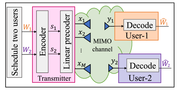
Figure 2: Two-user system architecture with MU–LP/SDMA.

The above contrasts with the optimal sum multiplexing gain $d_{\textnormal{s}}^{(\star)}$ of the two-user MISO BC, that is equal to 2, i.e., two interference-free streams can be transmitted. This can be achieved by performing conventional MU–LP, illustrated in Fig. 2. Recall MU–LP system model where $W_{1}$ and $W_{2}$ are independently encoded into streams $s_{1}$ and $s_{2}$ and respectively precoded by $\mathbf{p}_{1}$ and $\mathbf{p}_{2}$ such that the transmit signal is given by

$$\mathbf{x}=\mathbf{p}_{1}s_{1}+\mathbf{p}_{2}s_{2}.$$ (13)

At the receivers, $y_{k}=\mathbf{h}_{k}^{H}\mathbf{x}+n_{k}$, $k=1,2$, and $s_{1}$ and $s_{2}$ are respectively decoded by user-1 and user-2 by treating any residual interference as noise, leading to MU–LP rates

$$R_{1}^{(\textnormal{M})}=\log_{2}\left(1+C\right),R_{2}^{(\textnormal{M})}=\log_{2}\left(1+B\right),$$ (14)

with

$$C=\frac{\left|\mathbf{h}_{1}^{H}\mathbf{p}_{1}\right|^{2}}{1+\left|\mathbf{h}_{1}^{H}\mathbf{p}_{2}\right|^{2}},$$ (15)

and $B$ as specified in (4). It is then indeed sufficient to transmit two streams using uniform power allocation and Zero-Forcing Beamforming (ZFBF), so that $\mathbf{h}_{1}^{H}\mathbf{p}_{2}=\mathbf{h}_{2}^{H}\mathbf{p}_{1}=0$, to reap the sum multiplexing gain $d_{\textnormal{s}}^{(\textnormal{M})}=d_{\textnormal{s}}^{(\star)}=2$ and the MMF multiplexing gain $d_{\textnormal{mmf}}^{(\textnormal{M})}=d_{\textnormal{mmf}}^{(\star)}=1$ (i.e., each user gets one full interference-free stream). Indeed, with MU–LP, the sum-rate scales as $2\log_{2}(P)$ and the MMF rate as $\log_{2}(P)$ at high SNR [53, 54, 55]. Such sum-rate and MMF rate would always strictly outperform that of NOMA (and OMA) at high SNR. Since both OMA and NOMA achieve only half the (sum/MMF) multiplexing gain of MU–LP in the two-user MISO BC considered, it is not clear whether (and under what conditions) multi-antenna NOMA can outperform MU–LP and other forms of multi-user multi-antenna communication strategies, and if it does, whether multi-antenna NOMA is worth the associated increase in receiver complexity. The above discussion exposes some weaknesses of multi-antenna NOMA and highlights the uncertainty regarding the potential benefits of multi-antenna NOMA. Hence, in the following sections, we derive the multiplexing gains of generalized $K$-user multi-antenna NOMA, so as to better assess its potential.

Remark 2

It appears from (1) and (13) that the transmit signal vectors for 2-user MISO NOMA and 2-user MU–LP are the same, therefore giving the impression that NOMA is the same as MU–LP. This is obviously incorrect. Recall the major differences in the encoding and the decoding of NOMA and MU–LP:

• Encoding: In NOMA, $W_{1}$ is encoded into $s_{1}$ and $W_{2}$ is encoded into $s_{2}$ at a rate such that $s_{2}$ is decodable by both users, while $W_{1}$ and $W_{2}$ are independently encoded into streams $s_{1}$ and $s_{2}$ in MU–LP.

• Decoding: user-1 decodes $s_{1}$ and $s_{2}$ and user-2 decodes $s_{2}$ by treating $s_{1}$ as noise in NOMA while $s_{1}$ is decoded by user-1 by treating $s_{2}$ as noise and $s_{2}$ is decoded by user-2 by treating $s_{1}$ as noise in MU–LP.

Consequently the rate expressions (2), (3) and (14) are different, which therefore suggests that the best pair of precoders $\mathbf{p}_{1}$ and $\mathbf{p}_{2}$ that maximizes a given objective function (e.g. sum-rate, MMF rate, etc) would be different for NOMA and MU–LP. Choosing $\mathbf{p}_{1}$ and $\mathbf{p}_{2}$ according to ZFBF would commonly work reasonably well for MU–LP but would lead to $R_{2}^{(\textnormal{N})}=0$ in (3) for NOMA. Nevertheless, the above discussion on multiplexing gain loss of MISO NOMA always holds, even in the event where MISO NOMA is implemented with the best choice of precoders, since the above analysis for MISO NOMA is based on upperbound.

III $K$-User MISO NOMA with Perfect CSIT

We now study $K$-user MISO NOMA relying on perfect CSIT and derive the sum and MMF multiplexing gains.

III-A MISO NOMA System Model

We consider a $K$-user MISO NOMA scenario where a single transmitter equipped with $M$ transmit antennas serves $K$ single-antenna users indexed by $\mathcal{K}=\{1,\cdots,K\}$. The $K$ users are grouped into $1\leq G<K$ groups with groups indexed by $\mathcal{G}=\{1,\cdots,G\}$. There are $g$ users per group, i.e., we therefore assume for simplicity that $K=gG$. Users in group $i$ are indexed by $\mathcal{K}_{i}=\{ig-g+1,\cdots,ig\}$. Hence, $\mathcal{K}=\bigcup_{i\in\mathcal{G}}\mathcal{K}_{i}$ and $|\mathcal{K}_{i}|=g$. Without loss of generality, we assume that users 1, $g+1$, $2g+1$, …, $K-g+1$ are the “strong users” respectively in group 1 to $G$, and perform $g-1$ layers of SIC to fully decode the messages (and therefore remove interference) from the other $g-1$ users within the same group. Similarly, the second user in each group (i.e., $ig-g+2$ in group $i$) performs $g-2$ layers of SIC to fully decode messages from other $g-2$ users within the same group, and so on. The two most popular MISO NOMA strategies employ either $G=1$ [17, 18, 19, 20] or $G=K/2$ [23, 24, 25, 26, 27, 28] but we here keep here the scenario general for any value of $1\leq G<K$. The general architecture of MISO NOMA is illustrated in Fig. 3. The two-user building block in Section II can be viewed as a particular setup with $K=2$ and $G=1$.

At the transmitter, the messages $W_{1}$ to $W_{K}$ intended for user-1 to user-$K$, respectively, are encoded into $s_{1}$ to $s_{K}$. However, some of the messages in each group have to be encoded using codebooks shared by a subset of the users in that group so that they can be decoded and cancelled from the received signals at the co-scheduled users in that group. In particular, taking group 1 as an example, $W_{2}$ to $W_{g}$ are encoded using codebooks shared with user-1 such that user-1 can decode all of these $g-1$ messages. After encoding, the $K$ streams are linearly precoded by precoders $\mathbf{p}_{1}$ to $\mathbf{p}_{K}$, where $\mathbf{p}_{k}\in\mathbb{C}^{M}$ is the precoder of $s_{k}$, and superposed at the transmitter. The resulting transmit signal is

$$\mathbf{x}=\sum_{k=1}^{K}\mathbf{p}_{k}s_{k}.$$ (16)

Defining $\mathbf{s}=[s_{1},...,s_{K}]^{T}$ and assuming that $\mathbb{E}[\mathbf{s}\mathbf{s}^{H}]=\mathbf{I}$, the average transmit power constraint is written as $\sum_{k=1}^{K}P_{k}\leq P$, where $P_{k}=\left\|\mathbf{p}_{k}\right\|^{2}$.

At the receiver side, the signal received at user-$k$ is $y_{k}=\mathbf{h}_{k}^{H}\mathbf{x}+n_{k}$, $k\in\mathcal{K}$, where $\mathbf{h}_{k}$ is the channel vector of each user-$k$ perfectly known at the transmitter and that user, and $n_{k}\sim\mathcal{CN}(0,1)$ is the AWGN. By employing SIC, user-$j$ in group $i$ (i.e., $j\in\mathcal{K}_{i}$) decodes the messages of users-$\{k\mid k\geq j,k\in\mathcal{K}_{i}\}$ within the same user group in a descending order of the user index while treating the interference from users in different groups as noise. Under the assumption of Gaussian signalling and perfect SIC, the rate at user-$j,j\in\mathcal{K}_{i}$, to decode the message of user-$k,k\geq j,k\in\mathcal{K}_{i}$, is given by

$$R_{j,k}=\log_{2}\left(1+\frac{|\mathbf{h}_{j}^{H}\mathbf{p}_{k}|^{2}}{I_{j,k}^{(in)}+I_{j,k}^{(ou)}+1}\right),$$ (17)

where

$$I_{j,k}^{(in)}=\sum\limits_{m<k,m\in\mathcal{K}_{i}}|\mathbf{h}_{j}^{H}\mathbf{p}_{m}|^{2},I_{j,k}^{(ou)}=\sum\limits_{l\neq i,l\in\mathcal{G}}\sum\limits_{m\in\mathcal{K}_{l}}|\mathbf{h}_{j}^{H}\mathbf{p}_{m}|^{2}$$ (18)

are the intra-group interference and inter-group interference received at user-$k$, respectively. As the message of user-$k,k\in\mathcal{K}_{i}$, has to be decoded by users-$\{j|j\leq k,j\in\mathcal{K}_{i}\}$, to ensure decodability, the rate of user-$k$ should not exceed

$$R_{k}^{(\textnormal{N})}=\min_{j\leq k,j\in\mathcal{K}_{i}}R_{j,k}.$$ (19)

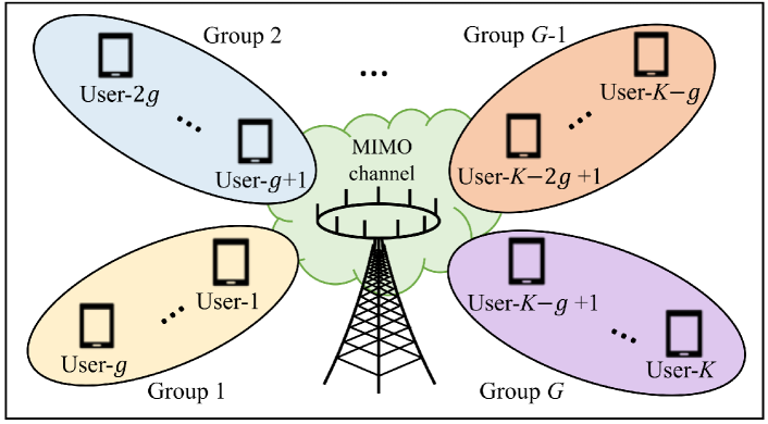
Figure 3: $K$-user system architecture with MISO NOMA (containing $G$ user groups and $g$ users within each group).

In the next subsection, we study the sum multiplexing gain and the MMF multiplexing gain of $K$-user MISO NOMA.

III-B Multiplexing Gains

The following proposition provides the sum multiplexing gain of MISO NOMA for perfect CSIT.

Proposition 1

The sum multiplexing gain of $K$-user MISO NOMA with $M$ transmit antennas, $G$ groups of $g=K/G$ users, and perfect CSIT is $d_{\textnormal{s}}^{(\textnormal{N})}=\min\left(M,G\right)$.

Proof: The proof is obtained by showing that an upper bound on the sum multiplexing gain is achievable. The upper bound is obtained by applying the MAC argument (used in (5)) to the strong user in each group and noticing that the sum-rate in groups 1 to $G$ is upper bounded as

$$\sum_{k=1}^{g}R_{k}^{(\textnormal{N})} \leq\log_{2}\left(1+\sum_{k=1}^{g}\left|\mathbf{h}_{1}^{H}\mathbf{p}_{k}\right|^{2}\right),$$ (20)

$$\sum_{k=g+1}^{2g}R_{k}^{(\textnormal{N})} \leq\log_{2}\left(1+\sum_{k=g+1}^{2g}\left|\mathbf{h}_{g+1}^{H}\mathbf{p}_{k}\right|^{2}\right),$$ (21)

$$\vdots$$

$$\sum_{k=K-g+1}^{K}R_{k}^{(\textnormal{N})} \leq\log_{2}\left(1+\sum_{k=K-g+1}^{K}\left|\mathbf{h}_{K-g+1}^{H}\mathbf{p}_{k}\right|^{2}\right).$$ (22)

Note that the left-hand sides of (20), (21), and (22) refer to the sum of the rates of the messages in group 1, 2, and $G$, respectively, but can also be viewed as the total rate to be decoded by user 1, $g+1$, and $K-g+1$ (since those users decode all the messages in their respective group). We now notice that the right-hand sides of (20), (21), and (22) scale as $\log_{2}(P)+\delta$ for large $P$ (following the same argument as in the two-user case). This implies that each group $i$ achieves at most a (group) sum multiplexing gain $d_{\textnormal{s},i}^{(\textnormal{N})}=\sum_{k=ig-g+1}^{ig}d_{k}^{(N)}$ of 1, i.e., at most one interference-free stream can be transmitted to each group. Summing up all inequalities, we obtain in the limit of large $P$ that

$$R_{\textnormal{s}}^{(\textnormal{N})}=\sum_{k=1}^{K}R_{k}^{(\textnormal{N})}\stackrel{{\scriptstyle P\nearrow}}{{\leq}}G\log_{2}(P)+\delta,$$ (23)

which shows that $d_{\textnormal{s}}^{(\textnormal{N})}=\sum_{i=1}^{G}d_{\textnormal{s},i}^{(\textnormal{N})}\leq G$. Additionally, since $d_{\textnormal{s}}^{(\textnormal{N})}\leq d_{\textnormal{s}}^{\star}=\min\left(M,K\right)$, we have $d_{\textnormal{s}}^{(\textnormal{N})}\leq\min\left(M,G\right)$.

The achievability part shows that $d_{\textnormal{s}}^{(\textnormal{N})}\geq\min\left(M,G\right)$. To this end, it is indeed sufficient to perform ZFBF and transmit $\min\left(M,G\right)$ interference-free streams to $\min\left(M,G\right)$ of the $G$ “strong users”. Combining the upper bound and achievability leads to the conclusion that $d_{\textnormal{s}}^{(\textnormal{N})}=\min\left(M,G\right)$. $\hfill\Box$

The following result derives the MMF multiplexing gain of MISO NOMA with perfect CSIT.

Proposition 2

The MMF multiplexing gain of $K$-user MISO NOMA with $M$ transmit antennas, $G$ groups of $g=K/G$ users and perfect CSIT is

$$d_{\textnormal{mmf}}^{(\textnormal{N})}=\left\{\begin{array}[]{l}\frac{1}{g},\hskip 5.69046ptM\geq K-g+1\\ 0,\hskip 5.69046ptM<K-g+1.\end{array}\right.$$ (24)

For $G=1$, i.e., $g=K$, $d_{\textnormal{mmf}}^{(\textnormal{N})}=\frac{1}{K}$.

Proof: Let us first consider $M\geq K-g+1$. The MMF multiplexing gain is always upperbounded by ignoring the inter-group interference, i.e., the $G$ groups are non-interfering. Following again the MAC argument, the sum multiplexing gain of one in each group can then be further split equally amongst the $g$ users, which leads to an upper bound on the MMF multiplexing gain of $\frac{1}{g}$. Achievability is simply obtained by designing the precoders using ZFBF to eliminate all inter-group interference, and allocating the power similarly to Subsection II-C, i.e., consider group 1 for simplicity, and allocate the power to user $k=1,\ldots,g$ as $O(P^{k/g})$, which leads to an SINR for user-$k$ scaling as $O(P^{1/g})$ and to an achievable MMF multiplexing gain of $\frac{1}{g}$. For $G=1$, one can simply allocate the power to user $k=1,\ldots,K$ as $O(P^{k/K})$, which leads to an achievable MMF multiplexing gain of $\frac{1}{K}$.

Let us now consider $M<K-g+1$. Take $M=K-g$ (any smaller $M$ cannot improve the multiplexing gain). Precoder $\mathbf{p}_{k}$ of any user-$k$ can be made orthogonal to the channel of $K-g-1$ co-scheduled users and will therefore cause interference to at least one user in another group. As a result, the MMF multiplexing gain collapses to 0. $\hfill\Box$

Remark 3

For the MMF multiplexing gain analysis, it should be noted that we consider one-shot transmission schemes with no time-sharing between strategies. This is suitable for systems with rigid scheduling and/or tight latency constraints, and also allows for simpler designs. This assumption is also commonly used in the NOMA literature [31, 32, 36, 48, 49].

IV $K$-user MISO NOMA with Imperfect CSIT

We now go one step further and extend the multiplexing gain analysis to the imperfect CSIT setting. The results in this section therefore generalize the results in the previous section (with perfect CSIT being a particular case of imperfect CSIT). In this section, the achievable rates are defined in the ergodic sense in a standard Shannon theoretic fashion, and the corresponding sum and MMF mutiplexing gains are defined similarly to Subsection II-B using ergodic rates. We first introduce the CSIT error model before deriving the multiplexing gains of MISO NOMA relying on imperfect CSIT.

IV-A CSIT Error Model

For each user, the transmitter acquires an imperfect estimate of the channel vector $\mathbf{h}_{k}$, denoted as $\hat{\mathbf{h}}_{k}$. The CSIT imperfection is modelled by

$$\mathbf{h}_{k}=\hat{\mathbf{h}}_{k}+\tilde{\mathbf{h}}_{k},$$ (25)

where $\tilde{\mathbf{h}}_{k}$ denotes the corresponding channel estimation error at the transmitter. For compactness, we define $\mathbf{H}=[\mathbf{h}_{1}\ldots\mathbf{h}_{K}]$, $\hat{\mathbf{H}}=[\hat{\mathbf{h}}_{1}\ldots\hat{\mathbf{h}}_{K}]$, and $\tilde{\mathbf{H}}=[\tilde{\mathbf{h}}_{1}\ldots\tilde{\mathbf{h}}_{K}]$, which implies $\mathbf{H}=\hat{\mathbf{H}}+\tilde{\mathbf{H}}$. The joint fading process is characterized by the joint distribution $f_{\mathbf{H},\hat{\mathbf{H}}}\big{(}\mathbf{H},\hat{\mathbf{H}}\big{)}$ of $\{\mathbf{H},\hat{\mathbf{H}}\}$, assumed to be stationary and ergodic . The joint distribution $f_{\mathbf{H},\hat{\mathbf{H}}}\big{(}\mathbf{H},\hat{\mathbf{H}}\big{)}$ is continuous and known to the transmitter. The ergodic rates capture the long-term performance over a long sequence of channel uses $\{\mathbf{H},\hat{\mathbf{H}}\}$ spanning almost all possible joint channel states.

For each user-$k$, we define the average channel (power) gain as $\Gamma_{k}=\mathbb{E}\big{\{}\left\|\mathbf{h}_{k}\right\|^{2}\big{\}}$. Similarly, we define $\hat{\Gamma}_{k}=\mathbb{E}\big{\{}\big{\|}\hat{\mathbf{h}}_{k}\big{\|}^{2}\big{\}}$ and $\tilde{\Gamma}_{k}=\mathbb{E}\big{\{}\big{\|}\tilde{\mathbf{h}}_{k}\big{\|}^{2}\big{\}}$. For many CSIT acquisition mechanisms [56], $\hat{\mathbf{h}}_{k}$ and $\tilde{\mathbf{h}}_{k}$ are uncorrelated according to the orthogonality principle [57]. By further assuming that $\hat{\mathbf{h}}_{k}$ and $\tilde{\mathbf{h}}_{k}$ have zero means, we have $\Gamma_{k}=\hat{\Gamma}_{k}+\tilde{\Gamma}_{k}$, based on which we can write $\hat{\Gamma}_{k}=(1-\sigma_{e,k}^{2})\Gamma_{k}$ and $\tilde{\Gamma}_{k}=\sigma_{e,k}^{2}\Gamma_{k}$ for some $\sigma_{e,k}^{2}\in[0,1]$. Note that $\sigma_{e,k}^{2}$ is the normalized estimation error variance for user-$k$’s CSIT, e.g., $\sigma_{e,k}^{2}=1$ corresponds to no instantaneous CSIT, while $\sigma_{e,k}^{2}=0$ represents perfect instantaneous CSIT.

For simplicity, we assume identical normalized CSIT error variances for all users, i.e., $\sigma_{e,k}^{2}=\sigma_{e}^{2}$ for all $k=1,\ldots,K$. To facilitate the multiplexing gain analysis, we assume that $\sigma_{e}^{2}$ scales with SNR as $\sigma_{e}^{2}=P^{-\alpha}$ for some CSIT quality parameter $\alpha\in[0,\infty)$ [59, 42, 58, 43, 55]. This is a convenient and tractable model extensively used in the information theoretic literature that allows us to assess the performance of the system in a wide range of CSIT quality conditions. Indeed, the larger $\alpha$, the faster the CSIT error decreases with the SNR. The two extreme cases, $\alpha=0$ and $\alpha=\infty$, correspond to no or constant CSIT (i.e. that does not scale or improve with SNR) and perfect CSIT, respectively. As far as the multiplexing gain analysis is concerned, however, we may truncate the CSIT quality parameter as $\alpha\in[0,1]$, where $\alpha=1$ amounts to perfect CSIT in the multiplexing gain sense. The regime $\alpha\in(0,1)$ corresponds to partial CSIT, resulting from imperfect CSI acquisition. The CSIT quality $\alpha$ can be interpreted in many different ways, but a plausible interpretation of $\alpha$ is related to the number of feedback bits, where $\alpha=0$ corresponds to a fixed number of feedback bits for all SNRs, $\alpha=\infty$ corresponds to an infinite number of feedback bits, and $0<\alpha<\infty$ reflects how quickly the number of feedback bits increases with the SNR. As a reference, a system like 4G and 5G use $\alpha=0$ when limited feedback (or codebook-based feedback) is used to report the CSI, since the number of feedback bits is constant and does not scale with SNR, e.g. 4 bits of CSI feedback in 4G LTE for $M=4$.

IV-B Multiplexing Gains

The following result quantifies the sum multiplexing gain of MISO NOMA for imperfect CSIT.

Proposition 3

The sum multiplexing gain of $K$-user MISO NOMA with $M$ transmit antennas, $G$ groups of $g=K/G$ users, and CSIT quality $0\leq\alpha\leq 1$ is $d_{\textnormal{s}}^{(\textnormal{N})}=\max\left(1,\min\left(M,G\right)\alpha\right)$.

Proof: Similarly to the proof of Proposition 1, let us look at the $G$ strong users, since they are the ones who have to decode all messages. We recall that $d_{\textnormal{s},i}^{(\textnormal{N})}=\sum_{k=ig-g+1}^{ig}d_{k}^{(N)}$ reflects the multiplexing gain of the total rate to be decoded by the strong user $ig-g+1$ in group $i$ as a consequence of the fact that this user decodes all $g$ messages in group $i$. Making use of the results of MU–LP in the $G$-user MISO BC with imperfect CSIT [43], we obtain $d_{\textnormal{s}}^{(\textnormal{N})}=\sum_{i=1}^{G}d_{\textnormal{s},i}^{(\textnormal{N})}=\sum_{k=1}^{K}d_{k}^{(N)}\leq\max\left(1,\min\left(M,G\right)\alpha\right)$.

The achievability part shows that $d_{\textnormal{s}}^{(\textnormal{N})}\geq\max\left(1,\min\left(M,G\right)\alpha\right)$. It is indeed sufficient to perform ZFBF and transmit $\min\left(M,G\right)$ streams, each at a power level of $P^{\alpha}/\min\left(M,G\right)$, to $\min\left(M,G\right)$ of the $G$ “strong users”. If $\min\left(M,G\right)\alpha<1$, one can simply transmit a single stream (i.e., perform OMA) and reap a sum multiplexing gain of 1. Combining the upper bound and achievability leads to the conclusion that we have $d_{\textnormal{s}}^{(\textnormal{N})}=\max\left(1,\min\left(M,G\right)\alpha\right)$. $\hfill\Box$

For $\alpha=1$ (perfect CSIT from a multiplexing gain perspective), Proposition 3 boils down to the perfect CSIT result in Proposition 1.

The following proposition provides the MMF multiplexing gain of MISO NOMA with imperfect CSIT.

Proposition 4

The MMF multiplexing gain of $K$-user MISO NOMA with $M$ transmit antennas, $G$ groups of $g=K/G$ users, and CSIT quality $0\leq\alpha\leq 1$ is

$$d_{\textnormal{mmf}}^{(\textnormal{N})}=\left\{\begin{array}[]{l}\frac{\alpha}{g},\hskip 8.5359ptG>1\>\textrm{and}\>M\geq K-g+1\\ 0,\hskip 11.38092ptG>1\>\textrm{and}\>M<K-g+1\\ \frac{1}{K},\hskip 6.544ptG=1.\end{array}\right.$$ (26)

The proof is relegated to Appendix A.

It is interesting to note that the sensitivity of the multiplexing gain of MISO NOMA to the CSIT quality $\alpha$ is different for $G>1$ and $G=1$. Indeed the sum and MMF multiplexing gains of MISO NOMA with $G>1$ decay as $\alpha$ decreases, while the multiplexing gains of MISO NOMA with $G=1$ are not affected by $\alpha$. This can be interpreted in two different ways. On the one hand, this suggests that MISO NOMA $G=1$ is inherently robust to CSIT imperfections since the multiplexing gains are not affected by $\alpha<1$. On the other hand, this also reveals that MISO NOMA with $G=1$ is unable to exploit the presence of CSIT since its multiplexing gains are the same as in the absence of CSIT ($\alpha=0$).

V Baseline Scheme I:
Conventional Multi-user Linear Precoding

The first baseline to assess the performance of multi-antenna NOMA is conventional Multi-User Linear Precoding. In the sequel, we recall the multiplexing gains achieved by MU–LP.

V-A MU–LP System Model

Following Subsection III-A, we consider a $K$-user MISO BC with one transmitter equipped with $M$ transmit antennas and $K$ single-antenna users. As per Fig. 4, the messages $W_{1},\ldots,W_{K}$ respectively for user-1 to user-$K$ are independently encoded into $s_{1}$ to $s_{K}$, which are then mapped to the transmit antennas through the precoders $\mathbf{p}_{1},\ldots,\mathbf{p}_{K}$. The resulting transmit signal is $\mathbf{x}=\sum_{k=1}^{K}\mathbf{p}_{k}s_{k}.$

The signal received at user-$k$ is $y_{k}=\mathbf{h}_{k}^{H}\mathbf{x}+n_{k}$ with $n_{k}\sim\mathcal{CN}(0,1)$. Each user-$k$ directly decodes the intended message $W_{k}$ by treating the interference from other users as noise. Under the assumption of Gaussian signalling, the rate of user-$k$ for $k\in\mathcal{K}$ is given by

$$R_{k}^{(\textnormal{M})}=\log_{2}\left(1+\frac{\left|\mathbf{h}_{k}^{H}\mathbf{p}_{k}\right|^{2}}{1+\sum_{q\neq k}\left|\mathbf{h}_{k}^{H}\mathbf{p}_{q}\right|^{2}}\right).$$ (27)

The sum-rate of MU–LP is therefore $R_{\mathrm{s}}^{(\textnormal{M})}=\sum_{k=1}^{K}R_{k}^{(\textnormal{M})}$, and the MMF rate of MU–LP is given as $R_{\mathrm{mmf}}^{(\textnormal{M})}=\min_{k=1,\ldots,K}R_{k}^{(\textnormal{M})}$.

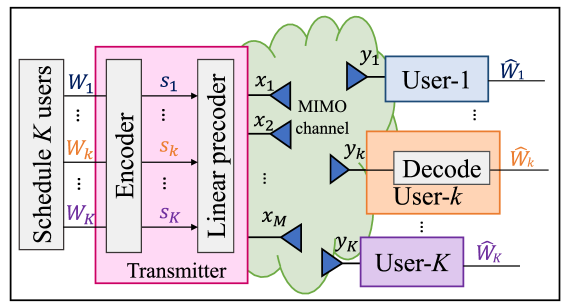
Figure 4: $K$-user system architecture with MU–LP. Receiver architecture is illustrated for user-$k$ though the same applies to other users, i.e. all $K$ users are equipped with a decoder that maps the received signal into an estimated message by treating residual interference as noise.

V-B Multiplexing Gains with Perfect CSIT

We recall the sum multiplexing gain and the MMF multiplexing gain of MU–LP with perfect CSIT from [54] and [51], respectively.

Proposition 5

The sum multiplexing gain of $K$-user MU–LP with $M$ transmit antennas and perfect CSIT is $d_{\textnormal{s}}^{(\textnormal{M})}=\min\left(M,K\right)$.

This result is simply achieved by choosing the MU–LP precoders based on ZFBF and transmitting $\min\left(M,K\right)$ interference-free streams. Note that $\min\left(M,K\right)$ is also the optimal sum multiplexing gain of the $K$-user MISO BC [54]. In other words, $d_{\textnormal{s}}^{(\textnormal{M})}=d_{\textnormal{s}}^{(\star)}=\min\left(M,K\right)$.

Proposition 6

The MMF multiplexing gain of the $K$-user MU–LP with $M$ transmit antennas and perfect CSIT is

$$d_{\textnormal{mmf}}^{(\textnormal{M})}=\left\{\begin{array}[]{l}1,\hskip 5.69046ptM\geq K\\ 0,\hskip 5.69046ptM<K.\end{array}\right.$$ (28)

When $M\geq K$, ZFBF can be used to fully eliminate interference. On the other hand, for $M<K$ interference cannot be eliminated anymore and $d_{\textnormal{mmf}}^{(\textnormal{M})}$ collapses, therefore leading to a rate saturation at high SNR.

V-C Multiplexing Gains with Imperfect CSIT

We use the CSIT error model introduced in Subsection IV-A. We recall the sum multiplexing gain and the MMF multiplexing gain of MU–LP with imperfect CSIT from [43] and [44, 60], respectively.

Proposition 7

The sum multiplexing gain of the $K$-user MU–LP with $M$ transmit antennas and CSIT quality $0\leq\alpha\leq 1$ is $d_{\textnormal{s}}^{(\textnormal{M})}=\max\left(1,\min\left(M,K\right)\alpha\right)$.

This result is simply achieved by choosing the MU–LP precoders based on ZFBF and transmitting $\min\left(M,K\right)$ streams, each with power level $P^{\alpha}/\min\left(M,K\right)$. This enables each stream to reap a multiplexing gain of $\alpha$ and therefore a sum multiplexing gain of $\min\left(M,K\right)\alpha$. If $\min\left(M,K\right)\alpha<1$, one can simply transmit a single stream (i.e., perform OMA) and reap a sum multiplexing gain of 1.

Comparing Propositions 5 and 7, we note that imperfect CSIT leads to a reduction of the sum multiplexing gain. For $\alpha=1$ (perfect CSIT in a multiplexing gain sense), Proposition 7 matches Proposition 5. Importantly, in contrast to the $K$-user MISO BC with perfect CSIT setting where MU–LP achieves the information theoretic optimal sum multiplexing gain $d_{\textnormal{s}}^{(\textnormal{M})}=d_{\textnormal{s}}^{(\star)}$, in the imperfect CSIT setting, MU–LP does not achieve the information theoretic optimal sum multiplexing gain [58, 43].

Proposition 8

The MMF multiplexing gain of the $K$-user MU–LP with $M$ transmit antennas and CSIT quality $0\leq\alpha\leq 1$ is

$$d_{\textnormal{mmf}}^{(\textnormal{M})}=\left\{\begin{array}[]{l}\alpha,\hskip 5.69046ptM\geq K\\ 0,\hskip 5.69046ptM<K.\end{array}\right.$$ (29)

This is achieved by performing ZFBF when $M\geq K$. When $M<K$, rate saturation occurs (similarly to the perfect CSIT setting).

VI Baseline Scheme II: Rate-Splitting

The second baseline to assess multi-antenna NOMA performance is multi-antenna Rate-Splitting (RS) and Rate-Splitting Multiple Access (RSMA) for the multi-antenna BC [41, 42, 43, 44, 45, 46, 47]. This literature leverages and extends the concept of RS, originally developed in [61] for the two-user single-antenna interference channel, to design multi-antenna non-orthogonal transmission strategies for the multi-antenna BC.

VI-A Rate-Splitting System Model

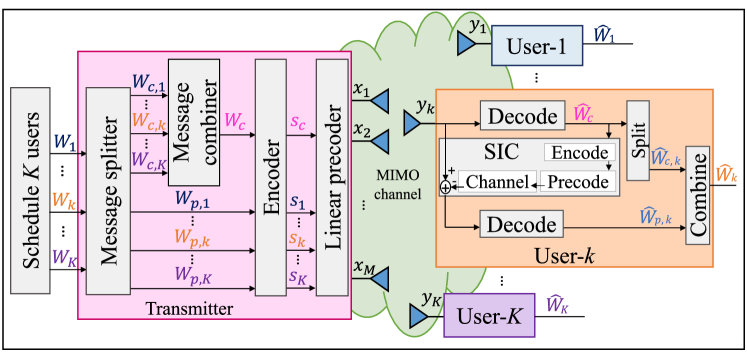
Figure 5: $K$-user system architecture with 1-layer rate-splitting. Receiver architecture is illustrated for user-$k$ though the same applies to other users.

We consider again a MISO BC consisting of one transmitter with $M$ antennas and $K$ single-antenna users. As per Fig. 5, the architecture relies on rate-splitting of messages $W_{1}$ to $W_{K}$ intended for user-1 to user-$K$, respectively. To that end, message $W_{k}$ of user-$k$ is split into a common part $W_{\mathrm{c},k}$ and a private part $W_{\mathrm{p},k}$. The common parts $W_{\mathrm{c},1},\ldots,W_{\mathrm{c},K}$ of all users are combined into the common message $W_{\mathrm{c}}$, which is encoded into the common stream $s_{\mathrm{c}}$ using a codebook shared by all users. Hence, $s_{\mathrm{c}}$ is a common stream required to be decoded by all users, and contains parts of messages $W_{1}$ to $W_{K}$ intended for user-1 to user-$K$, respectively. The private parts $W_{\mathrm{p},1},\ldots,W_{\mathrm{p},K}$, respectively containing the remaining parts of messages $W_{1}$ to $W_{K}$, are independently encoded into the private stream $s_{1}$ for user-1 to $s_{K}$ for user-$K$. Out of the $K$ messages, $K+1$ streams $s_{\mathrm{c}},s_{1},\ldots,s_{K}$ are therefore created. The streams are linearly precoded such that the transmit signal is given by

$$\mathbf{x}=\mathbf{p}_{\mathrm{c}}s_{\mathrm{c}}+\sum_{k=1}^{K}\mathbf{p}_{k}s_{k}.$$ (30)

Defining $\mathbf{s}=[s_{\mathrm{c}},s_{1},\ldots,s_{K}]^{T}$ and assuming that $\mathbb{E}[\mathbf{s}\mathbf{s}^{H}]=\mathbf{I}$, the average transmit power constraint is written as $P_{\mathrm{c}}+\sum_{k=1}^{K}P_{k}\leq P$, where $P_{\mathrm{c}}=\left\|\mathbf{p}_{\mathrm{c}}\right\|^{2}$ and $P_{k}=\left\|\mathbf{p}_{k}\right\|^{2}$.

At each user-$k$, the common stream $s_{\mathrm{c}}$ is first decoded into $\widehat{W}_{\mathrm{c}}$ by treating the interference from the private streams as noise. Using SIC, $\widehat{W}_{\mathrm{c}}$ is re-encoded, precoded, and subtracted from the received signal, such that user-$k$ can decode its private stream $s_{k}$ into $\widehat{W}_{\mathrm{p},k}$ by treating the remaining interference from the other private stream as noise. User-$k$ reconstructs the original message by extracting $\widehat{W}_{\mathrm{c},k}$ from $\widehat{W}_{\mathrm{c}}$, and combining $\widehat{W}_{\mathrm{c},k}$ with $\widehat{W}_{\mathrm{p},k}$ into $\widehat{W}_{k}$. Assuming proper Gaussian signalling, the rate of the common stream is given by

$$R_{\mathrm{c}}=\min_{k=1,...,K}\log_{2}\left(1+\frac{\left|\mathbf{h}_{k}^{H}\mathbf{p}_{\mathrm{c}}\right|^{2}}{1+\sum_{q=1}^{K}\left|\mathbf{h}_{k}^{H}\mathbf{p}_{q}\right|^{2}}\right).$$ (31)

Assuming perfect SIC, the rates of the private streams are obtained as

$$R_{k}=\log_{2}\left(1+\frac{\left|\mathbf{h}_{k}^{H}\mathbf{p}_{k}\right|^{2}}{1+\sum_{q\neq k}\left|\mathbf{h}_{k}^{H}\mathbf{p}_{q}\right|^{2}}\right).$$ (32)

The rate of user-$k$ is given by $R_{k}+R_{\mathrm{c},k}$ where $R_{\mathrm{c},k}$ is the rate of the common part of the $k$th user’s message, i.e., $W_{\mathrm{c},k}$, and it satisfies $\sum_{k=1}^{K}R_{\mathrm{c},k}=R_{\mathrm{c}}$. The sum-rate is therefore simply written as $R_{\mathrm{s}}^{(\textnormal{R})}=\sum_{k=1}^{K}(R_{k}+R_{\mathrm{c},k})=R_{\mathrm{c}}+\sum_{k=1}^{K}R_{k}$, and the MMF rate is written as $R_{\mathrm{mmf}}^{(\textnormal{R})}=\min_{k=1,\ldots,K}R_{k}+R_{\mathrm{c},k}$.

The above RS architecture is called 1-layer RS since it only relies on a single common stream and a single layer of SIC at each user as illustrated in Fig. 5.

VI-B Multiplexing Gains with Perfect CSIT

We here summarize the sum and MMF multiplexing gains achieved by 1-layer RS with perfect CSIT.

Proposition 9

The sum multiplexing gain of the $K$-user 1-layer RS with $M$ transmit antennas and perfect CSIT is $d_{\textnormal{s}}^{(\textnormal{R})}=\min\left(M,K\right)$.

Proof: Since MU–LP is a subscheme of 1-layer RS, it is sufficient to design the private precoders using ZFBF and allocate zero power to the common stream at high SNR. Note that $d_{\textnormal{s}}^{(\textnormal{R})}=d_{\textnormal{s}}^{(\textnormal{M})}=d_{\textnormal{s}}^{(\star)}=\min\left(M,K\right)$. $\hfill\Box$

Proposition 10

The MMF multiplexing gain of the $K$-user 1-layer RS with $M$ transmit antennas and perfect CSIT is

$$d_{\textnormal{mmf}}^{(\textnormal{R})}=\left\{\begin{array}[]{l}1,\hskip 34.14322ptM\geq K\\ \frac{1}{1+K-M},\hskip 5.69046ptM<K.\\ \end{array}\right.$$ (33)

The MMF multiplexing gain of 1-layer RS was derived and proved in [51], under the same assumption as in Remark 3. Readers are referred to [51] for more details of the proof of Proposition 10.

VI-C Multiplexing Gains with Imperfect CSIT

Again, we use the CSIT error model introduced in Subsection IV-A. We recall the sum multiplexing gain of RS with imperfect CSIT from [43].

Proposition 11

The sum multiplexing gain of $K$-user 1-layer RS with $M$ transmit antennas and CSIT quality $0\leq\alpha\leq 1$ is $d_{\textnormal{s}}^{(\textnormal{R})}=1+\left(\min\left(M,K\right)-1\right)\alpha$.

Achievability of $d_{\textnormal{s}}^{(\textnormal{R})}$ in Proposition 11 is obtained by using random precoding to design $\mathbf{p}_{c}$ with power level $P_{c}=O(P)$, transmitting $\min(M,K)$ private streams and using ZFBF to design the precoders of those $\min(M,K)$ private streams, each with power level $P_{k}=O(P^{\alpha})$. From the SINR expressions at the right-hand side of (31), it follows that the received SINR of the common stream at each user scales as $O(P^{1-\alpha})$, leading to the multiplexing gain of $1-\alpha$ achieved by the common stream $s_{c}$. By performing ZFBF, the transmitter transmits $\min\left(M,K\right)$ interference-free private streams. The received SINR of each private stream scales as $O(P^{\alpha})$ leading to multiplexing gain $\alpha$. Hence, we obtain the sum multiplexing gain of $1+(\min\left(M,K\right)-1)\alpha$.

Importantly, for the underloaded regime $M\geq K$, 1-layer RS achieves the information theoretic optimal sum multiplexing gain $d_{\textnormal{s}}^{(\textnormal{M})}=d_{\textnormal{s}}^{(\star)}$ in the imperfect CSIT setting [58, 43]. Hence, 1-layer RS attains the optimal sum multiplexing gain in both perfect CSIT and imperfect CSIT (underloaded regime). Actually, for $M\geq K$, 1-layer RS is optimal, achieving the maximum multiplexing gain region of the underloaded $K$-user MISO BC with imperfect CSIT [62, 63].

This optimality of RS (including 1-layer RS), shown through multiplexing gain analysis, is very significant since it implies that one cannot find any other scheme achieving a better multiplexing gain region in multi-antenna BC. As a consequence of this optimality, MU–LP and multi-antenna NOMA will always incur a multiplexing gain loss or at best will achieve the same multiplexing gain as RS for both perfect and imperfect CSIT.

Proposition 12

The MMF multiplexing gain of $K$-user 1-layer RS with $M$ transmit antennas and CSIT quality $0\leq\alpha\leq 1$ is

$$d_{\textnormal{mmf}}^{(\textnormal{R})}=\left\{\begin{array}[]{l}\frac{1+(K-1)\alpha}{K},\hskip 5.69046ptM\geq K\\ \frac{1+(M-1)\alpha}{K},\hskip 5.69046ptM<K\>\textnormal{and}\>\alpha\leq\frac{1}{1+K-M}\\ \frac{1}{1+K-M},\hskip 11.38092ptM<K\>\textnormal{and}\>\alpha>\frac{1}{1+K-M}.\\ \end{array}\right.$$ (34)

The MMF multiplexing gain of 1-layer RS with imperfect CSIT was derived in [60] (by considering the specific case where there is a single user per group), under the same assumption as in Remark 3. Readers are referred to [60] for more details of the proof of Proposition 12.

This highlights that when $M<K$, the CSIT quality $\alpha$ can be reduced to $\frac{1}{1+K-M}$ without impacting the MMF multiplexing gain of 1-layer RS.

Following our discussion of Proposition 11, we know that when $M\geq K$, the respective multiplexing gains of the common and each private streams are $1-\alpha$ and $\alpha$. The MMF multiplexing gain when $M\geq K$ is achieved by evenly sharing the common stream among users, which is the sum of evenly allocated multiplexing gain of the common stream $\frac{1-\alpha}{K}$ and the multiplexing gain of one private stream $\alpha$, yielding $\frac{1+(K-1)\alpha}{K}$.

When $M<K$, the achievability is obtained by partitioning users into two subsets $\mathcal{K}_{1}$ and $\mathcal{K}_{2}$ with set size of $|\mathcal{K}_{1}|=M$ and $|\mathcal{K}_{2}|=K-M$. Users in $\mathcal{K}_{1}$ are served via the common and private streams while users in $\mathcal{K}_{2}$ are served using the common stream only. Random precoding and ZFBF are respectively used for the common stream and the private streams with power allocation $P_{c}=O(P)$ and $P_{k}=O(P^{\beta}),\forall k\in\mathcal{K}_{1}$. It may be readily shown that the respective multiplexing gains of the common stream and each private stream are given by $1-\beta$ and $\min\{\alpha,\beta\}$, respectively. By further introducing a fraction $z\in[0,1]$ to specify the fraction of the rate of the common stream allocated to the users in the two subsets, we obtain that the respective sum multiplexing gains of the common stream for the users in $\mathcal{K}_{1}$ and $\mathcal{K}_{2}$ are $z(1-\beta)$ and $(1-z)(1-\beta)$, respectively. By equally dividing the multiplexing gain of the common stream between the users in the two subsets, the multiplexing gain of each user in $\mathcal{K}_{2}$ is $d_{k,2}=\frac{(1-z)(1-\beta)}{K-M}$, and the multiplexing gain of each user in $\mathcal{K}_{1}$ is $d_{k,1}=\min\{\alpha,\beta\}+\frac{z(1-\beta)}{M}$. The MMF multiplexing gain among the users is $\max_{z}\min\{d_{k,1},d_{k,2}\}$. When $\beta=\alpha$, the optimal rate allocation factor $z^{\star}$ is obtained when $\frac{(1-z)(1-\alpha)}{K-M}=\frac{z(1-\alpha)}{M}+\alpha$. We have $z^{\star}=\frac{(1-\alpha-\alpha K+\alpha M)M}{(1-\alpha)K}$ and the optimal MMF multiplexing gain is $\frac{1+(M-1)\alpha}{K}$. As $z^{\star}\in[0,1]$, we have $1-\alpha-\alpha K+\alpha M\geq 0$. Hence, when $\alpha\leq\frac{1}{1+K-M}$, $d_{\textnormal{mmf}}^{(\textnormal{R})}=\frac{1+(M-1)\alpha}{K}$. When $\beta<\alpha$ and $z=0$, the optimal power allocation $\beta^{\star}$ is obtained when $\frac{1-\beta}{K-M}=\beta$. We have $\beta^{\star}=\frac{1}{1+K-M}$ and the optimal MMF multiplexing gain is $\frac{1}{1+K-M}$. Hence, when $\alpha>\frac{1}{1+K-M}$, $d_{\textnormal{mmf}}^{(\textnormal{R})}=\frac{1}{1+K-M}$.

For $\alpha=1$, the results in Propositions 11 and 12 boil down to the perfect CSIT results in Propositions 9 and 10, respectively.

VII Shortcomings and Misconceptions of Multi-Antenna NOMA

In this section, we first compare the multiplexing gains of multi-antenna NOMA to those of the MU–LP and 1-layer RS baselines. The sum and MMF multiplexing gains of multi-antenna NOMA, MU–LP, and 1-layer RS for both perfect and imperfect CSIT are summarized in Table II. The objective of this section is to identify under which conditions NOMA provides performance gains/losses over the two baselines. We then use these comparisons to reveal several misconceptions and shortcomings of multi-antenna NOMA.

TABLE II: Comparison of sum and MMF multiplexing gains of different strategies with perfect and imperfect CSIT

Strategy	Sum/MMF Multiplexing Gain	Perfect CSIT	Imperfect CSIT
MISO NOMA	$d_{\textnormal{s}}^{(\textnormal{N})}$	$\min\left(M,G\right)$	$\max\left(1,\min\left(M,G\right)\alpha\right)$
	$d_{\textnormal{mmf}}^{(\textnormal{N})}$	$\left\{\begin{matrix}\frac{1}{g},&M\geq K-g+1\\ \\ 0,&M<K-g+1\end{matrix}\right.$	$\left\{\begin{matrix}\frac{\alpha}{g},&G>1\>\textnormal{and}\>M\geq K-g+1\\ 0,&G>1\>\textnormal{and}\>M<K-g+1\\ \frac{1}{K},&G=1\end{matrix}\right.$
MU–LP	$d_{\textnormal{s}}^{(\textnormal{M})}$	$\min\left(M,K\right)$	$\max\left(1,\min\left(M,K\right)\alpha\right)$
	$d_{\textnormal{mmf}}^{(\textnormal{M})}$	$\left\{\begin{matrix}1,&M\geq K\\ \\ 0,&M<K\end{matrix}\right.$	$\left\{\begin{matrix}\alpha,&M\geq K\\ \\ 0,&M<K\end{matrix}\right.$
1-layer RS	$d_{\textnormal{s}}^{(\textnormal{R})}$	$\min\left(M,K\right)$	$1+\left(\min\left(M,K\right)-1\right)\alpha$
	$d_{\textnormal{mmf}}^{(\textnormal{R})}$	$\left\{\begin{matrix}1,&M\geq K\\ \\ \frac{1}{1+K-M},&M<K\end{matrix}\right.$	$\left\{\begin{matrix}\frac{1+(K-1)\alpha}{K},&M\geq K\\ \frac{1+(M-1)\alpha}{K},&M<K\>\textnormal{and}\>\alpha\leq\frac{1}{1+K-M}\\ \frac{1}{1+K-M},&M<K\>\textnormal{and}\>\alpha>\frac{1}{1+K-M}\end{matrix}\right.$

VII-A NOMA vs. Baseline I (MU–LP)

We show in the following corollaries that MISO NOMA can achieve a performance gain over MU–LP but it may also incur a performance loss, depending on the values of $M$, $K$, $G$, and $\alpha$.

The performance (expressed in terms of multiplexing gain) gain/loss of multi-antenna NOMA vs. MU–LP is obtained by comparing Propositions 3 and 7 (for sum multiplexing gain), and Propositions 4 and 8 (for MMF multiplexing gain), which are summarized in Corollary 1, and 2 ($G=1$), and 3 ($G>1$), respectively. For the MMF multiplexing gain with imperfect CSIT, we consider $G=1$ and $G>1$ in two different corollaries.

Corollary 1

The sum multiplexing gain comparison between MISO NOMA and MU–LP is summarized in (35). MISO NOMA never achieves a sum multiplexing gain higher than MU–LP.

$$d_{\textnormal{s}}^{(\textnormal{N})}-d_{\textnormal{s}}^{(\textnormal{M})}\left\{\begin{matrix}<0,&\textrm{if }([\min\left(M,G\right)\alpha<1]\cap[\min\left(M,K\right)\alpha>1])\cup([M>G]\cap[\min\left(M,G\right)\alpha\geq 1])\\ =0,&\textrm{if }(\min\left(M,K\right)\alpha\leq 1)\cup([\min\left(M,G\right)\alpha\geq 1]\cap[M\leq G]).\end{matrix}\right.$$ (35)

Corollary 1 shows that MISO NOMA can achieve a lower or the same sum multiplexing gain compared to MU–LP, but cannot outperform MU–LP.

If $\alpha=1$ (perfect CSIT), Corollary 1 boils down to $d_{\textnormal{s}}^{(\textnormal{N})}<d_{\textnormal{s}}^{(\textnormal{M})}$ whenever $M>G$, and $d_{\textnormal{s}}^{(\textnormal{N})}=d_{\textnormal{s}}^{(\textnormal{M})}$ whenever $M\leq G$. This is instrumental as it says that the slope of the sum-rate of MISO NOMA at high SNR will be strictly lower than that of MU–LP (i.e., the sum-rate of MISO NOMA will grow more slowly than that of MU–LP) whenever the number of transmit antennas is larger than the number of groups, and hence in this case, MU–LP is guaranteed to outperform MISO NOMA at high SNR. Consequently, in the massive MIMO regime where $M$ grows large, MISO NOMA would achieve a sum multiplexing gain strictly lower than MU–LP (and the role of NOMA in massive MIMO is therefore questionable as highlighted in [66]). If $G=1$ as in e.g., [17, 18, 19, 20], MISO NOMA always incurs a sum multiplexing gain loss compared to MU–LP irrespective of $M$ (except in single-antenna systems when $M=1$). In other words, from a sum multiplexing gain perspective, one cannot find any multi-antenna configuration at the transmitter, i.e., any value of $M$, that would motivate the use MISO NOMA with $G=1$ compared to MU–LP. If $G=K/2$ as in [23, 24, 25, 26, 27], MISO NOMA incurs a sum multiplexing gain loss compared to MU–LP whenever $M>K/2$. In other words, from a sum multiplexing gain perspective, the only multi-antenna deployments for which MISO NOMA with $G=K/2$ would not incur a multiplexing gain loss (but no improvement either) over MU–LP is when $M\leq K/2$.

If $\alpha<1$ (imperfect CSIT), a sum multiplexing gain loss of MISO NOMA over MU–LP occurs in two different scenarios: 1) medium CSIT quality setting with $\frac{1}{\min\left(M,K\right)}<\alpha<\frac{1}{\min\left(M,G\right)}$ or 2) sufficiently large number of antennas and high CSIT quality with $M>G$ and $\alpha\geq\frac{1}{\min\left(M,G\right)}$. In other scenarios where the CSIT quality is poor $\alpha\leq\frac{1}{\min\left(M,K\right)}$ or the CSIT quality is good $\alpha\geq\frac{1}{\min\left(M,G\right)}$ but the number of transmit antennas is low $M\leq G$, MISO NOMA and MU–LP achieve the same sum multiplexing gains.

Corollary 2

The MMF multiplexing gain comparison between MISO NOMA with $G=1$ and MU–LP is summarized as follows

$$d_{\textnormal{mmf}}^{(\textnormal{N})}-d_{\textnormal{mmf}}^{(\textnormal{M})}\left\{\begin{matrix}<0,&\textrm{if }(M\geq K)\cap(\alpha>\frac{1}{K})\\ =0,&\textrm{if }(M\geq K)\cap(\alpha=\frac{1}{K})\\ >0,&\textrm{if }(M<K)\cup((M\geq K)\cap(\alpha<\frac{1}{K})).\end{matrix}\right.$$ (36)

Corollary 3

The MMF multiplexing gain comparison between MISO NOMA with $G>1$ and MU–LP is summarized as follows

$$d_{\textnormal{mmf}}^{(\textnormal{N})}-d_{\textnormal{mmf}}^{(\textnormal{M})}\left\{\begin{matrix}<0,&\textrm{if }M\geq K\\ =0,&\textrm{if }M<K-g+1\\ >0,&\textrm{if }K>M\geq K-g+1.\end{matrix}\right.$$ (37)

Corollaries 2 and 3 show that MISO NOMA can achieve either a higher or a lower MMF multiplexing gain compared to MU–LP, depending on the values of $M$, $G$, $K$, and $\alpha$.

If $\alpha=1$ (perfect CSIT), with $G=1$ as in e.g., [17, 18, 19, 20], $d_{\textnormal{mmf}}^{(\textnormal{N})}>d_{\textnormal{mmf}}^{(\textnormal{M})}$ whenever $M<K$, and incurs an MMF multiplexing loss otherwise ($M\geq K$). With $G=K/2$ as in [23, 24, 25, 26, 27], $d_{\textnormal{mmf}}^{(\textnormal{N})}<d_{\textnormal{mmf}}^{(\textnormal{M})}$ whenever $M\geq K$, and $d_{\textnormal{mmf}}^{(\textnormal{N})}>d_{\textnormal{mmf}}^{(\textnormal{M})}$ whenever $K>M\geq K-1$, and $d_{\textnormal{mmf}}^{(\textnormal{N})}=d_{\textnormal{mmf}}^{(\textnormal{M})}$ whenever $M<K-1$. In other words, from an MMF multiplexing gain perspective, the multi-antenna deployments for which MISO NOMA with $G=1$ and $G=K/2$ can outperform or achieve the same performance as MU–LP when $M<K$.

If $\alpha<1$ (imperfect CSIT), we note from Corollary 3, that for $G>1$, CSIT quality $\alpha$ does not affect the operational regimes where MISO NOMA outperforms/incurs a loss compared to MU–LP. This is different from $G=1$ where the condition for $d_{\textnormal{mmf}}^{(\textnormal{N})}<d_{\textnormal{mmf}}^{(\textnormal{M})}$ is a function of $\alpha$ in Corollary 2. MISO NOMA incurs an MMF multiplexing loss whenever the number of antenna and the CSIT quality are sufficiently large, i.e., $M\geq K$ and $\alpha>\frac{1}{K}$.

VII-B NOMA vs. Baseline II (RS)

We show in the following corollaries that, for all $M$, $K$, $\alpha$, 1-layer RS (that relies on a single SIC at each user) achieves the same or higher (sum and MMF) multiplexing gains than the best of the MISO NOMA schemes (i.e., whatever $G$ and the number of SICs). In other words, 1-layer RS outperforms (multiplexing gain-wise) MISO NOMA and simultaneously requires fewer SICs (only one) than MISO NOMA. Hence, employing MISO NOMA over 1-layer RS can only cause a multiplexing gain loss and/or a complexity increase at the receiver.

The performance loss of MISO NOMA vs. RS is obtained by comparing Propositions 3 and 11 (for the sum multiplexing gain), and Propositions 4 and 12 (for the MMF multiplexing gain), and is summarized in Corollaries 4, and 5 ($G=1$), and 6 ($G>1$), respectively.

Corollary 4

The sum multiplexing gain comparison between MISO NOMA and 1-layer RS is summarized as follows

$$d_{\textnormal{s}}^{(\textnormal{N})}-d_{\textnormal{s}}^{(\textnormal{R})}\left\{\begin{matrix}<0,&\textrm{if }(0<\alpha<1)\cup([\alpha>0]\cap[M>G])\\ =0,&\textrm{if }(\alpha=0)\cup([\alpha=1]\cap[M\leq G]).\end{matrix}\right.$$ (38)

MISO NOMA never achieves a sum multiplexing gain higher than 1-layer RS.

If $\alpha=1$ (perfect CSIT), Corollary 4 boils down to $d_{\textnormal{s}}^{(\textnormal{N})}<d_{\textnormal{s}}^{(\textnormal{R})}$, whenever $M>G$, and $d_{\textnormal{s}}^{(\textnormal{N})}=d_{\textnormal{s}}^{(\textnormal{R})}$ whenever $M\leq G$.

Corollary 5

The MMF multiplexing gain comparison between MISO NOMA with $G=1$ and 1-layer RS is summarized as follows

$$d_{\textnormal{mmf}}^{(\textnormal{N})}-d_{\textnormal{mmf}}^{(\textnormal{R})}\left\{\begin{matrix}<0,&\textrm{if }(\alpha>0)\cap(M>1)\\ =0,&\textrm{if }(\alpha=0)\cup(M=1).\end{matrix}\right.$$ (39)

MISO NOMA with $G=1$ never achieves an MMF multiplexing gain higher than 1-layer RS.

Corollary 6

The MMF multiplexing gain comparison between MISO NOMA with $G>1$ and 1-layer RS is summarized in (40). MISO NOMA with $G>1$ never achieves an MMF multiplexing gain larger than 1-layer RS.

$$d_{\textnormal{mmf}}^{(\textnormal{N})}-d_{\textnormal{mmf}}^{(\textnormal{R})}\left\{\begin{matrix}<0,&\textrm{if }(M\neq K-g+1)\cup([]M=K-g+1]\cap[\alpha<1])\\ =0,&\textrm{if }(M=K-g+1)\cap(\alpha=1).\end{matrix}\right.$$ (40)

If $\alpha=1$ (perfect CSIT), Corollaries 5 and 6 simply boil down to $d_{\textnormal{mmf}}^{(\textnormal{N})}<d_{\textnormal{mmf}}^{(\textnormal{R})}$, whenever $M\neq K-g+1$, and $d_{\textnormal{mmf}}^{(\textnormal{N})}=d_{\textnormal{mmf}}^{(\textnormal{R})}$, whenever $M=K-g+1$.

Recalling again from [62, 63, 64, 65] that RS achieves the optimal multiplexing gain region in multi-antenna BC with imperfect CSIT, and multi-antenna NOMA (and MU–LP/MU-MIMO) will therefore always incur a multiplexing gain loss compared to RS.

VII-C Misconceptions of Multi-Antenna NOMA

The comparisons with the MU–LP and 1-layer RS baselines reveal that depending on the particular setting NOMA may incur a multiplexing gain loss at the additional expense of an increased receiver complexity, as detailed in the following.

First, NOMA is an inefficient strategy to exploit the spatial dimensions. This issue could already be observed from the two-user MISO case with perfect CSIT, where NOMA limits the sum multiplexing gain to one, same as OMA, which is only half of the sum multiplexing gain obtained with MU–LP. Moreover, even when considering a fair metric such as MMF, NOMA limits the MMF multiplexing gain to $\frac{1}{2}$, which is again only half of the MMF multiplexing gain obtained by MU–LP.

In the general $K$-user case, it is clear from Corollaries 1 and 4 that NOMA incurs a loss in sum multiplexing gain in most scenarios, and the best NOMA can achieve is the same sum multiplexing gain as the baselines in some specific configurations. NOMA with $G=1$ achieves $d_{\textnormal{s}}^{(\textnormal{N})}=1$ irrespectively of the number of transmit antennas $M$, i.e., it achieves the same sum multiplexing gain as OMA and the same as a single-antenna transmitter (hence, wasting the transmit antenna array). NOMA with $G=K/2$ achieves $d_{\textnormal{s}}^{(\textnormal{N})}=\min\left(M,K/2\right)$ with $\alpha=1$. On the other hand, MU–LP and 1-layer RS achieve the full sum multiplexing gain $d_{\textnormal{s}}^{(\textnormal{M})}=\min\left(M,K\right)$ with $\alpha=1$.

Considering the MMF multiplexing gain of the general $K$-user case, the situation appears to be better for NOMA. Assuming $\alpha=1$, from Corollaries 2 and 3, we observe that NOMA incurs a loss compared to MU–LP in the underloaded regime $M\geq K$ but outperforms MU–LP in the overloaded regime. In particular, NOMA with $G=1$ achieves a higher MMF multiplexing gain than NOMA wtih $G=K/2$ and MU–LP whenever $M<K-1$. Hence, though the receiver complexity increases of NOMA does not pay off in the underloaded regime, it appears to pay off in the overloaded regime (since $G=1$ with more SICs outperforms $G=K/2$ with fewer SICs). Nevertheless, the MMF multiplexing gain of NOMA with $G=1$ is independent of $M$, suggesting again that the spatial dimensions are not properly exploited. This can indeed be seen from Corollary 5 where NOMA is consistently outperformed by 1-layer RS, i.e., the increase in MMF multiplexing gain attained by NOMA ($G=1$) over MU–LP is actually marginal in light of the complexity increase, and is much lower than what can be achieved by 1-layer RS with just a single SIC operation. In other words, while NOMA has some merits over MU–LP in the overloaded regime, NOMA makes an inefficient use of the multiple antennas, and fails to boost the MMF multiplexing gain compared to the 1-layer RS baseline.

We note that the above observations hold for both the perfect and imperfect CSIT settings. Nevertheless, it is interesting to stress that the sensitivity to the CSIT quality $\alpha$ differs largely between MU–LP, NOMA with $G>1$, NOMA with $G=1$, and 1-layer RS. Indeed the sum and MMF multiplexing gains of MU–LP, NOMA with $G>1$, and 1-layer RS decay as $\alpha$ decreases, while the multiplexing gains of NOMA with $G=1$ are not affected by $\alpha$. This can be interpreted in two different ways. On the one hand, this implies that NOMA with $G=1$ is inherently robust to CSIT imperfections since the multiplexing gains are unchanged. On the other hand, this means that NOMA with $G=1$ is unable to exploit the available CSIT since the resulting multiplexing gain is the same as in the absence of CSIT ($\alpha=0$). One can indeed see from the above Propositions and Corollaries that the sum and MMF multiplexing gains for 1-layer RS with imperfect CSIT are clearly larger than those of MU–LP and NOMA. In other words, NOMA and MU–LP are inefficient in fully exploiting the available CSIT in multi-antenna settings.

We conclude from the theoretical results and above discussions that NOMA fails to efficiently exploit the multiplexing gain of the multi-antenna BC and is an inefficient strategy to exploit the spatial dimensions and the available CSIT, especially compared to the 1-layer RS baseline. The first misconception behind NOMA is to believe that because NOMA is capacity achieving in the single-antenna BC, NOMA is an efficient strategy for multi-antenna settings. As a consequence, the single-antenna NOMA principle has been applied to multi-antenna settings without recognizing that such a strategy would waste the primary benefit of using multiple antennas, namely the capability of transmitting multiple interference-free streams. In contrast to NOMA, other non-orthogonal transmission strategies such as 1-layer RS do not lead to any sum multiplexing gain loss. On the contrary, 1-layer RS achieves the information theoretic optimal sum multiplexing gain in both perfect and imperfect CSIT scenarios (and therefore has the capability of transmitting the optimal number of interference-free streams). 1-layer RS also achieves higher MMF multiplexing gains than NOMA and MU–LP.

Second, the multiplexing gain loss of NOMA is encountered despite the increased receiver complexity. In the two-user MISO BC with perfect CSIT, MU–LP does not require any SIC receiver to achieve the optimal sum multiplexing gain of two (assuming $M>1$) and a MMF multiplexing gain of one, while NOMA requires one SIC and only provides half the (sum and MMF) multiplexing gains of MU–LP. This is surprising since one would expect a performance gain from an increased architecture complexity. Here instead, NOMA brings together a complexity increase at the receivers and a (sum and MMF) multiplexing gain loss compared to MU–LP, therefore highlighting that the SIC receiver is inefficiently exploited.

This inefficient use of SIC in NOMA also persists in the general $K$-user scenario. Recall that NOMA with $G$ groups requires $g-1$ layers of SIC at the receivers. Among the two popular NOMA architectures $G=1$ and $G=K/2$, the former requires an even higher number of SIC layers than the latter (namely $K-1$ for $G=1$ and 1 for $G=K/2$) and has an even lower sum multiplexing gain ($d_{\textnormal{s}}^{(\textnormal{N})}=1$ for $G=1$ and $d_{\textnormal{s}}^{(\textnormal{N})}=\min\left(M,K/2\right)$ for $G=K/2$ with $\alpha=1$). On the other hand, MU–LP achieves the full sum multiplexing $d_{\textnormal{s}}^{(\textnormal{M})}=\min\left(M,K\right)$ with $\alpha=1$ without any need for SIC. This highlights the inefficient (and detrimental) use of SIC receivers in NOMA: the higher the number of SICs, the lower the sum multiplexing gain!

Comparing to the 1-layer RS baseline further highlights the inefficient use of SIC in NOMA. We note that 1-layer RS causes a complexity increase at the receivers (due to the one SIC needed) but also an increase in the (sum and MMF) multiplexing gains compared to MU–LP (i.e., it is easy to see from Propositions 7, 8, 11, and 12 that the sum and MMF multiplexing gains with RS are always either identical to or higher than those with MU–LP). Hence, in contrast to NOMA, the SIC in 1-layer RS is beneficial since it boosts the (sum and MMF) multiplexing gains and therefore introduces a performance gain compared to (or at least maintains the same performance as) MU–LP. Actually, 1-layer RS achieves the information theoretic optimal sum multiplexing gain for imperfect CSIT, and does so with a single SIC per user. This shows that to achieve the information theoretic optimality, it is sufficient to use a single SIC per user. This is in contrast to NOMA whose sum multiplexing gain is far from optimal and for which the sum multiplexing gain decreases as the number of SICs increases. The inefficient use of SIC in NOMA is also obvious from the MMF multiplexing gain. Indeed, from Proposition 2 and 10 and Corollary 5, the single SIC in 1-layer RS achieves a much larger MMF multiplexing gain than the $K-1$ layers of SIC needed for NOMA with $G=1$. This again illustrates how inefficient the use of SIC in NOMA often is. It also shows that there exist non-orthogonal (RS-based) transmission strategies with better performance and lower receiver complexity requiring just a single SIC per user.

We conclude from the theoretical analysis and above discussion that NOMA often does not make efficient use of the SIC receivers compared to the considered baselines. The second misconception regarding multi-antenna NOMA is to believe that adopting SIC receivers always boosts the rate since the interference is fully cancelled at the receiver. Considering the two-user toy example, and comparing (2) and (14), the interference power term $\left|\mathbf{h}_{1}^{H}\mathbf{p}_{2}\right|^{2}$ appearing in the SINR of user-1 in the MU–LP rate has indeed disappeared in NOMA thanks to the SIC receiver, such that $R_{\textnormal{M},1}\leq R_{\textnormal{N},1}$. However, this comes at the cost of a reduced rate for user-2 since $R_{\textnormal{N},2}=\min\left(\log_{2}\left(1+A\right),R_{\textnormal{M},2}\right)\leq R_{\textnormal{M},2}$. In other words, for a given pair of precoders $\mathbf{p}_{1}$ and $\mathbf{p}_{2}$, NOMA increases the rate (or maintains the same rate) of user-1 but decreases the rate (or maintains the same rate) of user-2 compared to MU–LP.

Third, reflecting on the above two misconceptions, the NOMA design philosophy does not leverage the extensive research in multi-user MIMO, which has been fundamental to 4G and 5G in achieving the optimal sum multiplexing gain of multi-antenna BC with perfect CSIT and low-complexity transmitter and receiver architectures. The third misconception behind multi-antenna NOMA is to believe that, since NOMA is routinely compared to OMA in SISO BC, it is also sufficient to compare NOMA to OMA in multi-antenna settings to demonstrate its merits. In fact, the Corollaries in Sections VII-A and VII-B show that NOMA is far from being an efficient strategy if NOMA is compared to alternative baselines. Unfortunately, simply comparing with OMA has led the NOMA literature to the misleading conclusion that multi-antenna NOMA is an efficient strategy. It should therefore be stressed that comparing NOMA to OMA does not demonstrate the merits of NOMA in multi-antenna settings and most importantly, the baseline for any multi-antenna NOMA design, optimization, and evaluation should be MU–LP and RS, not simply OMA! In contrast to MISO NOMA, the gain of 1-layer RS over MU–LP is guaranteed, i.e., the rate of 1-layer RS is equal to or higher than that of MU–LP, since MU–LP is a particular instance of RS when no power is allocated to the common stream.

Fourth, the SISO BC is naturally overloaded (more users than the number of transmit antennas, namely one), and NOMA was therefore concluded to be suitable for overloaded scenarios. The fourth misconception behind multi-antenna NOMA is to believe that MISO NOMA is an efficient strategy for overloaded regimes, namely whenever $K>M$. The Corollaries in Subsections VII-A and VII-B nevertheless expose that this is incorrect. It is clear that NOMA incurs a sum multiplexing gain erosion compared to MU–LP and 1-layer RS whenever $M>G$. Such a loss can occur also in the overloaded regime, namely whenever we have $K>M>G$. Moreover, NOMA incurs an MMF multiplexing gain loss compared to 1-layer RS whenever $M\neq K-g+1$. Here again, such a loss occurs also in the overloaded regime. In contrast to NOMA (and MU–LP), 1-layer RS is an efficient strategy for both the underloaded and overloaded regimes. Though NOMA with $G=1$ was shown in Proposition 2 to achieve a non-vanishing MMF multiplexing gain of $1/K$ in the overloaded regime, this MMF multiplexing gain is considerably smaller than that of 1-layer RS, therefore highlighting the inefficiency of NOMA in the overloaded regime. In particular, we note that the MMF multiplexing gain of 1-layer RS increases with $M$ in contrast to that of NOMA with $G=1$ which is constant regardless of $M$.

TABLE III: Sum multiplexing gain with $K=6$ - perfect CSIT.

$M$	regime	$d_{\textnormal{s}}^{(\textnormal{N})}$​ ($G\!=\!1$)	$d_{\textnormal{s}}^{(\textnormal{N})}$​ ($G\!=\!3$)	$d_{\textnormal{s}}^{(\textnormal{M})},d_{\textnormal{s}}^{(\star)},d_{\textnormal{s}}^{(\textnormal{R})}$
1	O	1	1	1
2	O	1	2	2
3	O	1	3	3
4	O	1	3	4
5	O	1	3	5
$\geq 6$	U	1	3	6

O: Overloaded ($K>M$), U: Underloaded ($K\leq M$)

TABLE IV: MMF multiplexing gain with $K\!=\!6$ ​-​ perfect CSIT.

$M$	regime	$d_{\textnormal{mmf}}^{(\textnormal{N})}$​ ($G\!=\!1$)	$d_{\textnormal{mmf}}^{(\textnormal{N})}$​ ($G\!=\!3$)	$d_{\textnormal{mmf}}^{(\textnormal{M})}$	$d_{\textnormal{mmf}}^{(\textnormal{R})}$
1	O	$\nicefrac{{1}}{{6}}$	0	0	$\nicefrac{{1}}{{6}}$
2	O	$\nicefrac{{1}}{{6}}$	0	0	$\nicefrac{{1}}{{5}}$
3	O	$\nicefrac{{1}}{{6}}$	0	0	$\nicefrac{{1}}{{4}}$
4	O	$\nicefrac{{1}}{{6}}$	0	0	$\nicefrac{{1}}{{3}}$
5	O	$\nicefrac{{1}}{{6}}$	$\nicefrac{{1}}{{2}}$	0	$\nicefrac{{1}}{{2}}$
$\geq 6$	U	$\nicefrac{{1}}{{6}}$	$\nicefrac{{1}}{{2}}$	1	1

O: Overloaded ($K>M$), U: Underloaded ($K\leq M$)

VII-D Illustration of the Misconceptions with an Example

To illustrate the above discussion and make the statements more explicit based on numbers, we consider a MISO BC with $K=6$, and compare in Table III the sum multiplexing gains $d_{\textnormal{s}}^{(\textnormal{N})}$ of NOMA with $G=1$ and $G=3$ and the sum multiplexing gain of MU–LP $d_{\textnormal{s}}^{(\textnormal{M})}$ and 1-layer RS $d_{\textnormal{s}}^{(\textnormal{R})}$ (recall that $d_{\textnormal{s}}^{(\textnormal{M})}=d_{\textnormal{s}}^{(\textnormal{R})}=d_{\textnormal{s}}^{(\star)}$) as a function of $M$ for perfect CSIT. We observe that NOMA incurs a sum multiplexing gain reduction (highlighted in red in Table III) in the underloaded regime but also in the overloaded regime depending on the values of $M$ and $G$. Specifically, in this example with $K=6$, $G=1$ incurs a sum multiplexing erosion compared to MU–LP and 1-layer RS whenever $M\geq 2$ and $G=3$ whenever $M\geq 4$. This shows that in an overloaded regime associated with $M<K$, although $M$ is the limiting factor of the sum multiplexing gain in MU–LP and 1-layer RS, $\min\left(M,G\right)$ is the limiting factor in NOMA. Morever, Table III clearly illustrates that the higher the number of SICs in NOMA, the lower the sum multiplexing gain. NOMA with $G=1$ requires 5 layers of SIC to achieve a multiplexing gain $d_{\textnormal{s}}^{(\textnormal{N})}=1$, NOMA with $G=3$ requires 1 layer of SIC and achieves at most $d_{\textnormal{s}}^{(\textnormal{N})}=3$. On the other hand, MU–LP does not require any SIC and achieves the optimal sum multiplexing gain $d_{\textnormal{s}}^{(\star)}$ (that can be as high as 6). 1-layer RS achieves the same (and optimal) sum multiplexing gain as MU–LP.

Table IV highlights the MMF multiplexing gains of NOMA, MU–LP, and 1-layer RS for $K=6$ with perfect CSIT and stresses the significant benefit of 1-layer RS over NOMA and MU–LP. The entries highlighted in red relate to configurations for which 1-layer RS provides a multiplexing gain strictly higher than that of NOMA and MU–LP. Recall that 1-layer RS provides those multiplexing gains over NOMA and MU–LP with a single SIC per user!

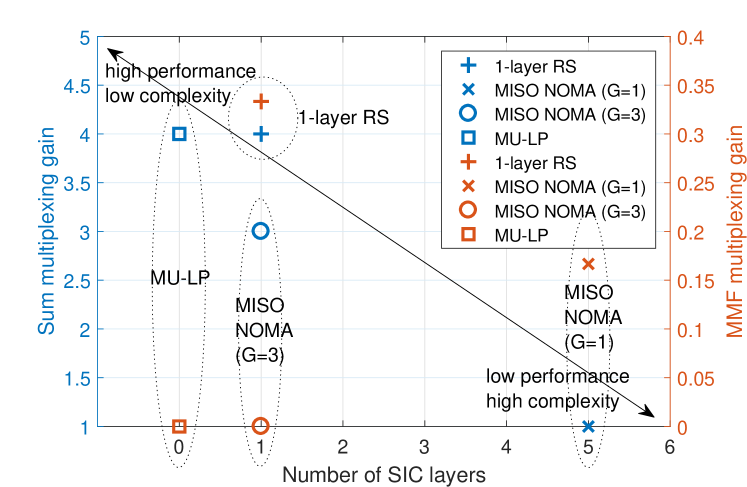
Figure 6: Multiplexing gains with single-antenna receivers and perfect CSIT vs. number of SIC layers for $M=4$, $K=6$.

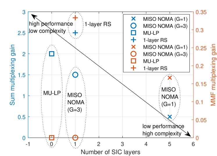
Figure 7: Multiplexing gains with single-antenna receivers and imperfect CSIT vs. number of SIC layers for $M=4$, $K=6$, $\alpha=0.5$.

In Fig. 6, we further illustrate the tradeoff between the multiplexing gains and the number of SIC layers for $M=4$, $K=6$ and perfect CSIT. We observe that 1-layer RS enables higher performance and lower receiver complexity compared to NOMA, stressing that the non-orthogonal transmission enabled by RS is much more efficient than NOMA. We see that NOMA with different $G$ is suited for very different settings in this $M=4$, $K=6$ configuration, namely NOMA with $G=3$ performs better in terms of sum multiplexing gain, whereas NOMA with $G=1$ achieves a higher MMF multiplexing gain. The baseline 1-layer RS achieves a higher performance for both metrics and entails a lower receiver complexity.

Though the above example was provided for perfect CSIT ($\alpha=1$), it is easy to calculate from the above propositions the multiplexing gains for the imperfect CSIT setting for a given CSIT quality $\alpha$. For imperfect CSIT, the strict superiority of 1-layer RS over MU–LP and NOMA will become much more apparent, as illustrated in Fig. 7 for $\alpha=0.5$.

VII-E Shortcomings of Multi-Antenna NOMA

The previous subsections have highlighted that comparing multi-antenna NOMA to MU–LP and 1-layer RS, instead of OMA, provides a completely different picture of the actual merits of multi-antenna NOMA. In view of the previous results highlighting the waste of multiplexing gain and the inefficient use of the SIC receivers by multi-antenna NOMA, we can ask ourselves multiple questions, which help to pinpoint the shortcomings and limitations of the multi-antenna NOMA design philosophy.

The first question is “What prevents multi-antenna NOMA from reaping the multiplexing gain of the system?” The answer lies in (5), and similarly in (20), (21), and (22). Equation (5) can be interpreted as the sum-rate of a two-user MAC with a single antenna receiver. Indeed, in (5), user-1 acts as the receiver of a two-user MAC whose effective SISO channels of both links are given by $\mathbf{h}_{1}^{H}\mathbf{p}_{2}$ and $\mathbf{h}_{1}^{H}\mathbf{p}_{1}$. Similarly, in (20), user-1 acts as the receiver of a $g$-user MAC whose effective SISO channels of the $g$ links are given by $\mathbf{h}_{1}^{H}\mathbf{p}_{k}$ for $k=1,\ldots,g$. Such a MAC is well known to have a sum multiplexing gain of one [15, 7]. The multiplexing gain losses compared to the MU–LP and 1-layer RS baselines therefore come from forcing one user to fully decode all streams in a group, i.e., its intended stream and the co-scheduled streams in the group. This is radically different from MU–LP where streams are encoded independently and each receiver decodes its intended stream treating any residual interference as noise. By contrast, in 1-layer RS, no user is forced to fully decode the co-scheduled streams since all private streams are encoded independently and each receiver decodes its intended private stream treating any residual interference from other private streams as noise.

The second question is “Does an increase in the number of SICs always come with a reduction in the sum multiplexing gain?” The answer is clearly no. This anomaly is deeply rooted in the way MISO NOMA was developed by applying single-antenna NOMA principle to multi-antenna settings. The proof of Proposition 1 indeed tells us that the fundamental principle of NOMA consisting in forcing one user in each group to fully decode the messages of $g-1$ co-scheduled users is an inefficient design in multi-antenna settings that leads to a sum multiplexing gain reduction in each group.

The third question is “Are non-orthogonal transmission strategies inefficient for multi-antenna settings?” The answer is no. As we have seen, there exist frameworks of non-orthogonal transmission strategies also relying on SIC, such as RS, that do not incur the limitations of multi-antenna NOMA and make efficient use of the non-orthogonality and SIC receivers in multi-antenna settings. The key for the design of such non-orthogonal strategies is not to fall into the trap of blindly applying the SISO NOMA principle to multi-antenna settings, and therefore constraining the strategy to always fully decode the message of other users. Non-orthogonal transmission strategies and multiple access need to be re-thought for multi-antenna settings and one such strategy is based on the multi-antenna Rate-Splitting (RS) and Rate-Splitting Multiple Access (RSMA) literature for multi-antenna BC .

The fourth question is “Since NOMA and RS both rely on SIC, is there any relationship between NOMA and RS?” The answer is yes in a two-user setting, but not necessarily in the general $K$-user case. In the two-user case, 1-layer RS is a superset of MU–LP, NOMA and multicasting, i.e., MU–LP, NOMA and multicasting are particular instances of 1-layer RS, as shown in [67] and in Table V and Fig. 8. Indeed, MU–LP is obtained as a special case from 1-layer RS by allocating no power to the common stream ($P_{\mathrm{c}}\!=\!0$) such that $W_{k}$ is encoded directly into $s_{k}$. No interference is decoded at the receiver using the common message, and the interference between $s_{1}$ and $s_{2}$ is fully treated as noise. NOMA is obtained by encoding $W_{2}$ entirely into $s_{\mathrm{c}}$ (i.e., $W_{\mathrm{c}}\!=\!W_{2}$) and $W_{1}$ into $s_{1}$, and turning off $s_{2}$ ($P_{2}\!=\!0$). In this way, user-1 fully decodes the interference created by the message of user-2. OMA is a sub-strategy of MU–LP and NOMA, which is encountered when only user-1 (with the stronger channel gain) is scheduled ($P_{\mathrm{c}}\!=\!0,P_{2}\!=\!0$). Multicasting is obtained when both $W_{1}$ and $W_{2}$ are entirely encoded into $s_{\mathrm{c}}$. In the $K$-user case, 1-layer RS is a superset of MU–LP since by turning off (i.e., allocating no power to) the common stream, 1-layer RS boils down to MU–LP. On the other hand, 1-layer RS is not a superset of NOMA. 1-layer RS and NOMA are particular instances/schemes of the RSMA framework based on the generalized RS relying on multiple layers of SIC at each receiver [47, 46, 68, 79], as illustrated in Fig. 9.

TABLE V: Messages-to-streams​ mapping​ in​ two-user​ MISO​ BC.

	$s_{1}$	$s_{2}$	$s_{c}$
MU–LP	$\,\,\quad\quad W_{1}\quad\quad\,\,$	$W_{2}$	–
NOMA	$W_{1}$	–	$W_{2}$
OMA	$W_{1}$	–	–
Multicasting	–	–	$W_{1},W_{2}$
RS	$W_{\mathrm{p},1}$	$W_{\mathrm{p},2}$	$W_{\mathrm{c},1},W_{\mathrm{c},2}$
	decoded by its intended user and		decoded by
	treated as noise by the other user		both users

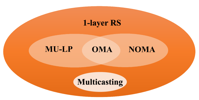
Figure 8: The relationship between existing strategies and 1-layer RS in two-user case. Each set illustrates the optimization space of the corresponding communication strategy. The optimization space of 1-layer RS is larger such that MU–LP, NOMA and multicasting are just subsets.

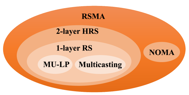
Figure 9: The relationship among existing strategies and the $K$-user RSMA framework.

The fifth question is “How does 1-layer RS achieve simultaneously higher multiplexing gains and a lower receiver complexity than NOMA?” In view of the previous sections, the key is to build non-orthogonal transmission strategies upon MU–LP (and therefore SDMA/multi-user MIMO) such that the performance benefits (including sum multiplexing gain) of MU–LP are guaranteed but extra performance (e.g., in MMF multiplexing gain) is observed by the use of SIC receivers. Indeed, a performance gain over MU–LP should be expected from a more complex receiver architecture in multi-antenna BC. To do so, one should enable the flexibility at the transmitter to encode messages such that parts of them can be decoded by all users using SIC while the remaining parts are decoded by their intended receivers and treated as noise by non-intended receivers. Hence, we provide the flexibility to partially decode interference and partially treat the remaining interference as noise. This contrasts with MU–LP where interference is always treated as noise, and with NOMA where interference is fully decoded. This flexibility is achieved by extending the concept of RS, originally developed in [61] for the two-user single-antenna interference channel, to the multi-antenna BC. To manage multi-user interference by partially decoding the interference and treating the remaining interference as noise, RS facilitates a complete message-to-streams mapping flexibility for each user to have part of its message transmitted in the common stream and the remaining part in one of the $K$ private streams. By adjusting the power levels of the common and private streams, one can adjust the amount of interference caused to the private streams such that its level is weak enough to be treated as noise. This contrasts with MU–LP where the communication strategy is fundamentally constrained such that the messages are mapped to private streams only (i.e., there is no common stream, and multi-user interference between private streams is treated as noise even when its level is not weak enough to be treated as noise), and with NOMA where the constraint is that the entire message of one of the users is mapped onto a common stream (e.g., $W_{2}$ mapped to $s_{2}$ decoded by both user-1 and 2 in Section II). These constraints imposed by MU–LP and NOMA are well illustrated by the message-to-stream mapping in Table V.

A consequence of the above flexibility is that by decreasing the amount of power allocated to the common stream, $K$-user 1-layer RS progressively converges to $K$-user MU–LP and in the limit where no power is allocated to the common stream, $K$-user 1-layer RS swiftly boils down to $K$-user MU–LP. Hence, 1-layer RS really builds upon MU–LP and MU–LP is a subscheme of 1-layer RS, which provides guarantee to 1-layer RS that its rate and multiplexing gains are always teh same or better than those of MU–LP. This is completely different from MISO NOMA. MISO NOMA does not build upon MU–LP. With $G$ groups, $K$-user MISO NOMA can boil down to $G$-user MU–LP by turning off the power to the weaker users in each group, but $K$-user MISO NOMA can mathematically never boil down to $K$-user MU–LP (recall footnote 11). The rate/multiplexing gains of $K$-user MISO NOMA can therefore be worse than that of $K$-user MU–LP.

Another interpretation arises by noting that MU–LP (and other form of multi-user MIMO), as one extreme, can be viewed as a full transmit-side interference management strategy. On the other extreme, NOMA can be seen as a full receiver-side interference cancellation strategy. In between stands RS that can be viewed as a smart combination of transmit-side and receive-side interference management/cancellation strategies where the contribution of the common stream is adjusted according to the level of interference that can be canceled by the receiver.

Consequently, RS is an enabler of a general class of communication strategies and can cover a wider set of communication strategies than SDMA and NOMA, which leads to significant multiplexing gain and complexity reduction benefits.

The sixth question is “Can we use other types of receivers than SIC for NOMA and RS and would the multiplexing gains be improved?” We can indeed use other types of receivers but the multiplexing gains will not improve. Instead of using stream-by-stream SIC, we can use any other joint (Maximum Likelihood) decoder. Hence a strong user in NOMA could use a joint decoder to decode its intended stream jointly with all other streams intended to its co-scheduled users in the same group. The multiplexing gains would not improve since the strong user would still act as the receiver of an effective MAC (as discussed in relationship with (5), (20), (21), and (22) and the first question) which limits the multiplexing gains. Similarly, in 1-layer RS, each user could use a joint decoder to decode its private stream jointly with the common stream and the multiplexing gains would not improve (recall that 1-layer RS already achieves the information theoretic optimal multiplexing gain region, hence any other scheme, receiver or multi-layer RS would not increase the multiplexing gains any further).

VIII Numerical Results

Through numerical evaluation, we illustrate the misconceptions and the shortcomings of MISO NOMA. Moreover, we show that, by adopting 1-layer RS, the optimal sum multiplexing gain of the MISO BC is guaranteed in both underloaded and overloaded deployments for both perfect and imperfect CSIT scenarios. Furthermore, results also demonstrate that the MMF multiplexing gain (and MMF rate) is significantly enhanced when using 1-layer RS compared to MU–LP and MISO NOMA, and the complexity of the receivers is reduced compared to MISO NOMA. In other words, our evaluations show that 1-layer RS makes a more efficient use of the spatial dimensions (multiplexing gains) and of the SIC receivers than MISO NOMA, and it is more robust to CSIT inaccuracy.

The following two precoder optimization problems are solved in the simulation for the $K$-user MISO NOMA system model specified in Section III-A. The first problem is maximizing the sum-rate of MISO NOMA subject to the transmit power constraint, which is given by

$$\max_{\mathbf{{P}}}\quad \sum_{k\in\mathcal{K}}R_{k}^{(\textnormal{N})}$$ (41a)

s.t. $$\text{tr}(\mathbf{P}\mathbf{P}^{H})\leq P$$ (41b)

where $R_{k}^{(\textnormal{N})}$ is the rate of user-$k$ in the MISO NOMA system as specified in (17)–(19). The second problem is maximizing the minimum rate subject to the transmit power constraint, which is formulated as

$$\max_{\mathbf{{P}}}\quad \min_{k\in\mathcal{K}}R_{k}^{(\textnormal{N})}$$ (42a)

s.t. $$\text{tr}(\mathbf{P}\mathbf{P}^{H})\leq P.$$ (42b)

The Weighted Minimum Mean Square Error (WMMSE) optimization framework proposed in [70] (originally developed for MU–LP) is extended to solve both problems (41) and (42). The details of the algorithm are specified in Appendix B. The optimization problems requiring interior-point methods are solved using the CVX toolbox [69].

We will assume $K=6$ in the simulations, so as to be able to relate the numerical results to the theoretical results of Table II. The channel $\mathbf{h}_{k}$ of user-$k$ has i.i.d. complex Gaussian entries drawn from the distribution $\mathcal{CN}(0,\sigma_{k}^{2})$. The presented results are averaged over 100 channel realizations.

The following five strategies are compared and analyzed for both perfect and imperfect CSIT:

• MISO NOMA ($G=3$): MISO NOMA ($G=3$) is the MISO NOMA strategy specified in Section III-A when $G=3$. Each user requires $\frac{K}{3}-1=1$ layer of SIC (since each user is possible to be selected as the “strong user" in the corresponding user group). Ideally, the sum-rate (or max-min) rate is maximized by solving (41) (or (42)) for all possible user grouping methods and decoding orders within each group. Due to the high computational complexity of jointly optimizing the precoders, grouping, and decoding order, we assume that the user grouping is fixed while the decoding order in each group $i$ is the ascending order of users’ channel strength $\|\mathbf{h}_{k}\|,\forall k\in\mathcal{K}_{i}$ in the following results. To keep aligned with the system model in Section III-A, user indices are updated within each group such that $\|\mathbf{h}_{k}\|\leq\|\mathbf{h}_{j}\|,\forall k<j$ and $k,j\in\mathcal{K}_{i}$. When the CSIT is imperfect, the decoding order follows the same method but based on $\|\hat{\mathbf{h}}_{k}\|,\forall k\in\mathcal{K}_{i}$.

• MISO NOMA ($G=1$): MISO NOMA ($G=1$) is the MISO NOMA strategy in Section III-A when $G=1$. Each user requires $K-1=5$ layers of SIC (since each user can potentially be selected as the “strong user"). There is no user grouping optimization issue at the transmitter since all users are assumed to be in the same user group. However, the decoding order at users should be jointly optimized with precoders in order to maximize sum-rate (or max-min rate), which however, is computationally prohibitive. Following the literature of single-cell MISO NOMA [19, 20], we assume that the decoding order is the ascending order of users’ channel strength $\|\mathbf{h}_{k}\|,\forall k\in\mathcal{K}$. User indices are updated such that $\|\mathbf{h}_{k}\|\leq\|\mathbf{h}_{j}\|,\forall k<j$ and $k,j\in\mathcal{K}$. Similarly, the decoding order follows the same method but based on $\|\hat{\mathbf{h}}_{k}\|,\forall k\in\mathcal{K}$ when the CSIT is imperfect.

• MU–LP: MU–LP is the baseline strategy studied in Section V. Each user directly decodes the intended stream by fully treating the interference as noise. The WMMSE algorithm specified in Appendix B can be applied and extended to solve the corresponding sum-rate and max-min problems of MU–LP [51, 70]. The transmitter and receiver complexity of MU–LP is low since there is no SIC is deployed at each user and no user grouping and decoding order optimization issue at the transmitter.

• Orthogonal Multiple Access (OMA): This is the single-user transmission where only the user with the highest channel strength is served.

• 1-layer RS: 1-layer RS is the RS strategy we specified in Section VI. The corresponding sum-rate and max-min rate maximization problems are solved by using the WMMSE algorithm proposed in [43, 51]. Compared with MISO NOMA schemes, the transmitter and receiver complexities of 1-layer RS are much reduced. Similarly to MU–LP, no user grouping and decoding order optimization is needed. Each user only requires a single layer of SIC.

VIII-A Perfect CSIT

Following [43], the initialization of the precoding matrix $\mathbf{P}$ in Algorithm 1 is designed by using Maximum Ratio Transmission (MRT) combined with Singular Value Decomposition (SVD). Specifically, the precoder for the message to be decoded by a group of users is designed based on the SVD of the channel matrix formed by the channel vectors of the corresponding users while the precoder for the message to be decoded by a single user is designed based on MRT. For example, when considering MISO NOMA ($G=3$), the message for user-$k,k\in\mathcal{K}_{i}$, is decoded by users-$\{j\mid j\leq k,j\in\mathcal{K}_{i}\}$. The precoders are initialized as $\mathbf{p}_{k}=\sqrt{p_{k}}\widehat{\mathbf{p}}_{k}$, where $\widehat{\mathbf{p}}_{k}$ is the largest left singular vector of the channel estimate ${\mathbf{H}}_{k}$ formed by channels $\{{\mathbf{h}}_{j}\mid j\leq k,j\in\mathcal{K}_{i}\}$. The precoder $\mathbf{p}_{k}$ of the stream to be decoded at last in each group is initialized as $\mathbf{p}_{k}=\sqrt{p_{k}}\frac{{\mathbf{h}}_{k}}{||{\mathbf{h}}_{k}||}$, where $p_{k}$ is the power allocated to the corresponding precoder $\mathbf{p}_{k}$ and it satisfies that $\sum_{k=1}^{K}p_{k}=P_{t}$.

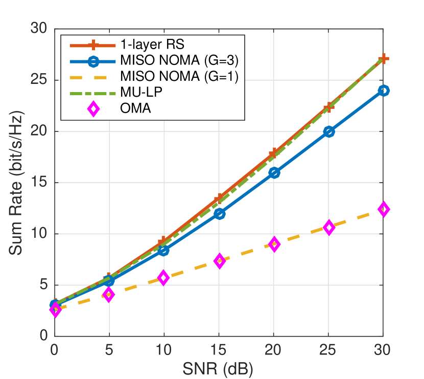
(a) $M=3$, $\sigma_{k}^{2}=1$

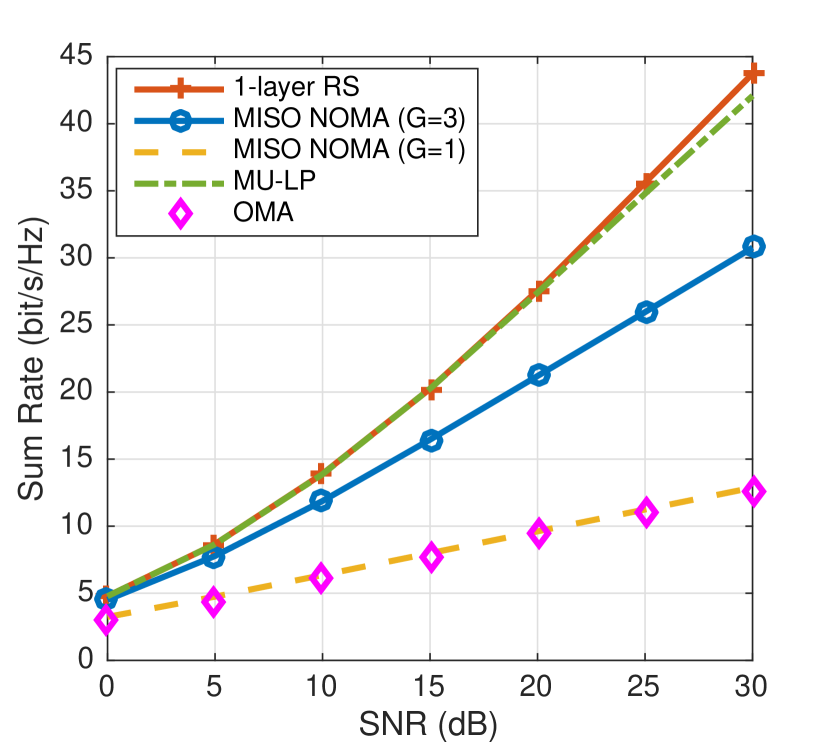
(b) $M=6,\sigma_{k}^{2}=1$

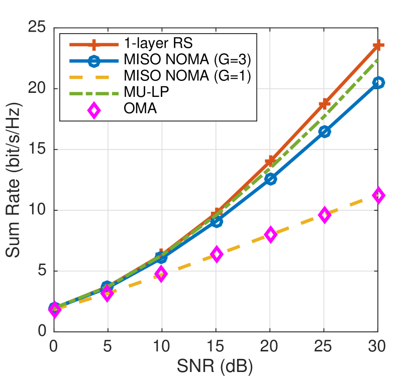
(c) $M=3,\sigma_{k}^{2}\in[0.1,1]$

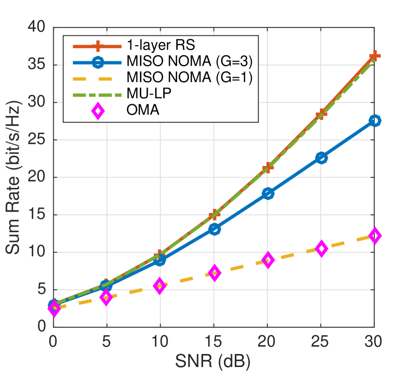
(d) $M=6,\sigma_{k}^{2}\in[0.1,1]$

Figure 10: Sum-rate vs. SNR comparison of different strategies, $K=6$.

Fig. 10 illustrates the sum-rate vs. SNR comparison of the five strategies considered when there are $K=6$ users and the number of transmit antennas is $M=3$ and $M=6$. In Fig. 10(a) and Fig. 10(b), all users have equal channel variances, i.e., $\sigma_{k}^{2}=1,\forall k\in\mathcal{K}$ while the users’ channel variances are randomly generated from $[0.1,1]$ in Fig. 10(c) and Fig. 10(d), i.e., $\sigma_{k}^{2}\in[0.1,1],\forall k\in\mathcal{K}$. In other words, the average channel strength disparities among users are randomly generated between 0 and 10 dB in Fig. 10(c) and Fig. 10(d). In the high SNR regime of each subfigure, the multiplexing gains of all strategies are found to match the theoretical sum multiplexing gains specified in Table III. Specifically, when $M=3,K=6$, the sum multiplexing gains of 1-layer RS, MU–LP, and MISO NOMA ($G=3$) in Fig. 10(a) and Fig. 10(c) approach $d_{\textnormal{s}}^{(\star)}=3$ (which is optimal). In Fig. 10(c) and Fig. 10(d) where $M=K=6$, the sum multiplexing gains of 1-layer RS and MU–LP are $d_{\textnormal{s}}^{(\star)}=6$. The sum multiplexing gain of MISO NOMA ($G=3$) remains 3. The sum multiplexing gains of MISO NOMA ($G=1$) and OMA are limited to 1 in all subfigures of Fig. 10. Therefore, MISO NOMA has a reduced sum multiplexing gain, inefficeintly makes use of the available multiple antennas and incurs a significant rate loss, especially at medium and high SNRs. It is not an efficient strategy for multi-antenna settings. The first misconception behind multi-antenna NOMA is confirmed.

As pointed out earlier in this section, the complexity of MISO NOMA at both the transmitter and the receiver is the highest among all strategies studied in this work. At the transmitter, the scheduling complexity is high since the user grouping and decoding order are required to be jointly optimized with the precoders. At the receivers, each user requires multiple layers of SIC and the number of SIC layers at each user increases with the number of users $K$ in the system. In addition to such a high complexity, as evident from Fig. 10, the sum-rate performance of MISO NOMA is worse than that of MU–LP which exhibits a much lower complexity at the transmitter and each receiver. Adopting SIC receivers does not always boost the rate performance. On the contrary, an inefficient and inappropriate use of SIC as in MISO NOMA can make the rate performance worse than simply not using SIC (as in MU–LP). This illustrates the second misconception behind multi-antenna NOMA.

We also observe from Fig. 10 that the sum-rate performance of OMA and MISO NOMA ($G=1$) is the worst, which is also reflected in their sum multiplexing gains. Hence, comparing MISO NOMA with OMA is not sufficient in multi-antenna settings. Both MU–LP and 1-layer RS should be considered as the baselines for all MISO NOMA schemes. This verifies the third misconception behind multi-antenna NOMA.

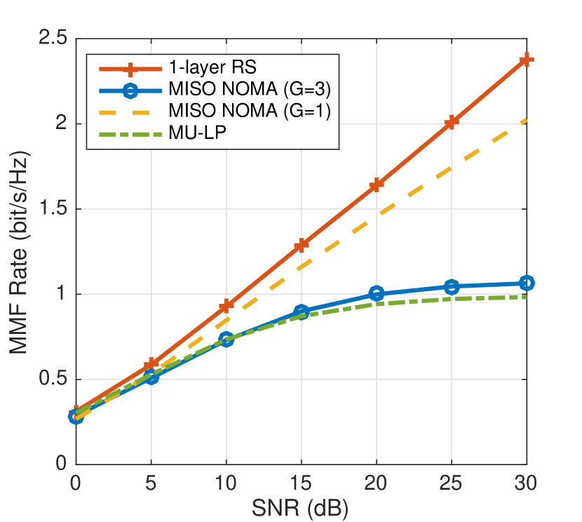
(a) $M=3$

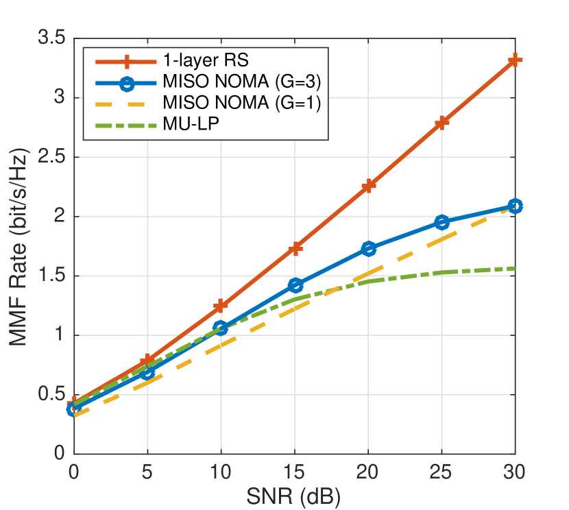
(b) $M=4$

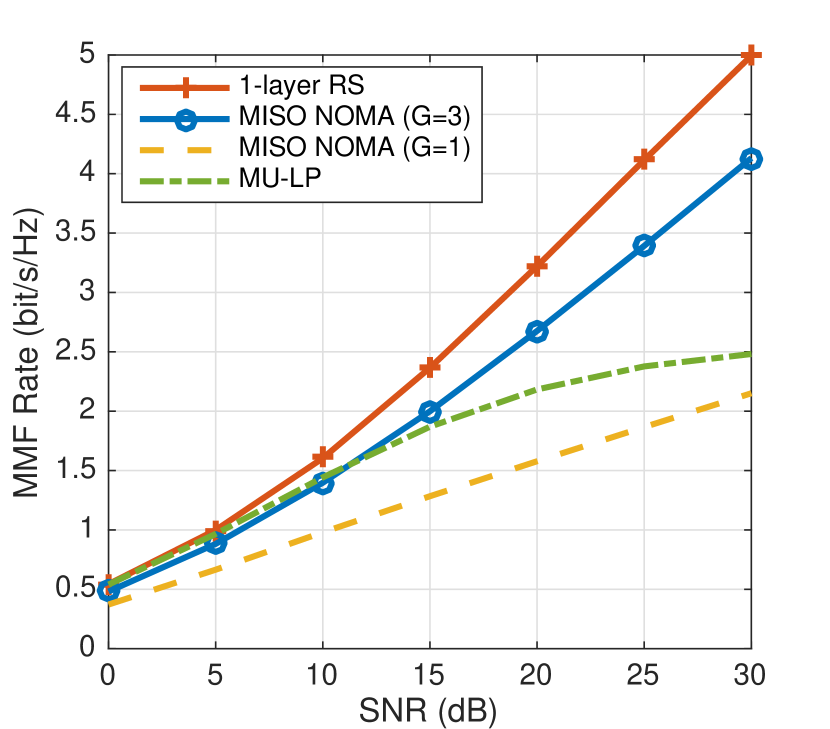
(c) $M=5$

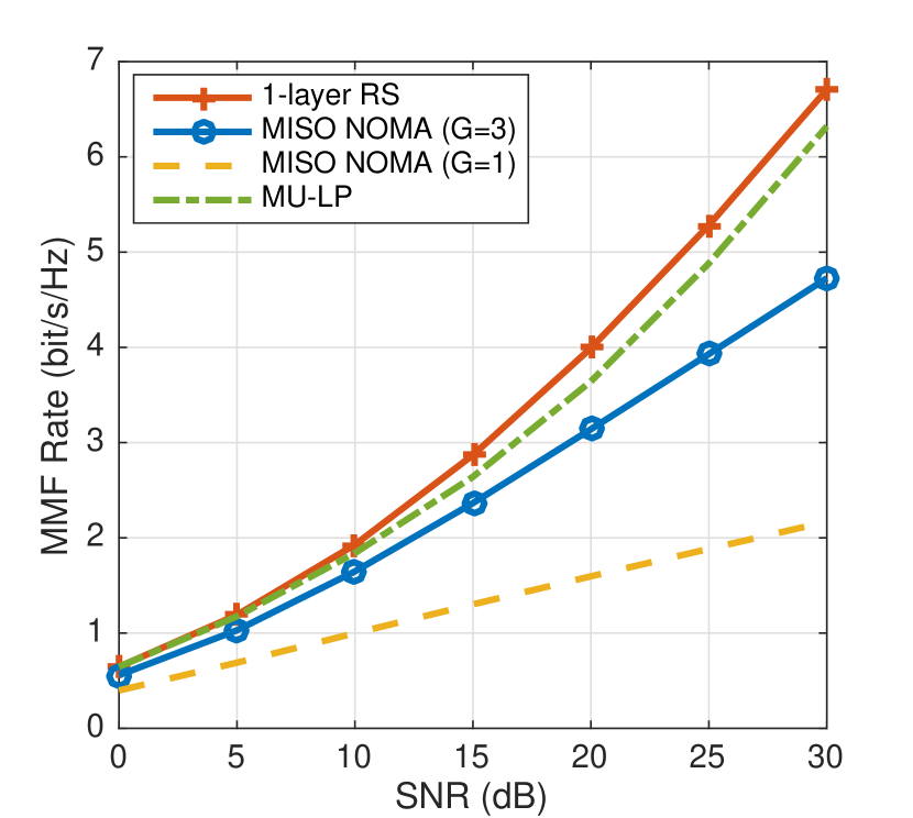
(d) $M=6$

Figure 11: Max-min rate vs. SNR comparison of different strategies, $K=6$, $\sigma_{k}^{2}=1,\forall k\in\mathcal{K}$.

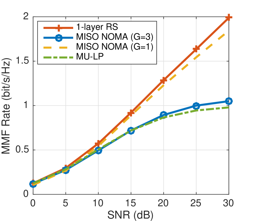
(a) $M=3$

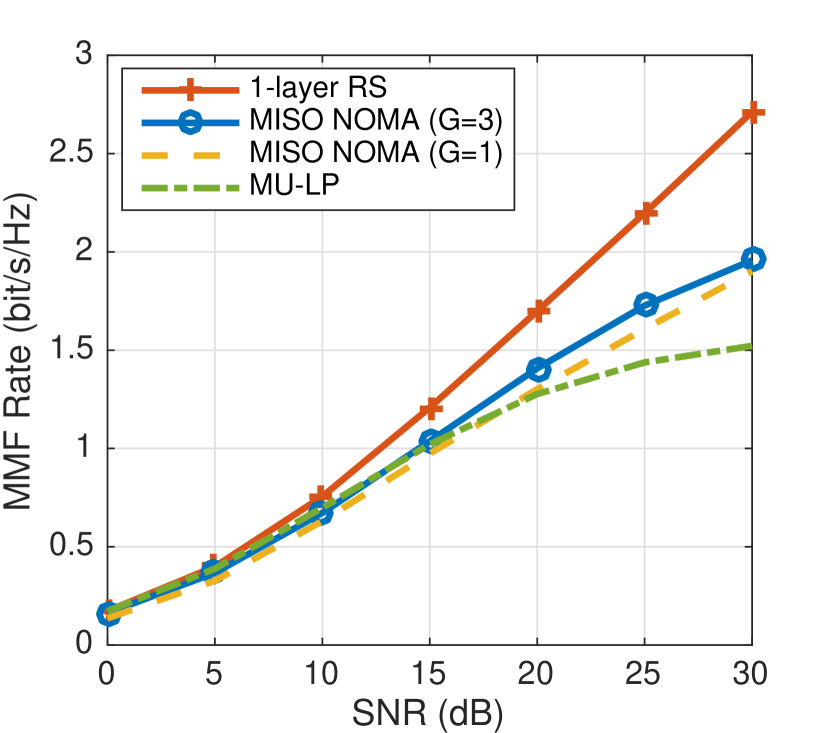
(b) $M=4$

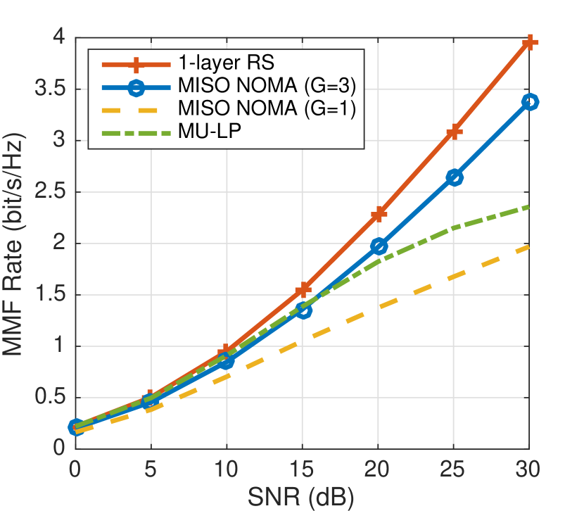
(c) $M=5$

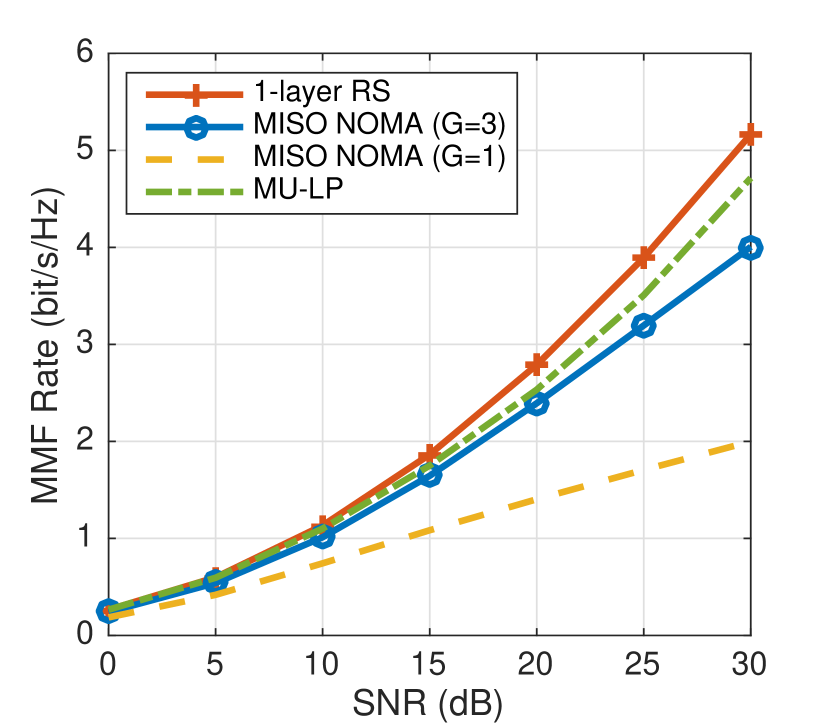
(d) $M=6$

Figure 12: Max-min rate vs. SNR comparison of different strategies, $K=6$, $\sigma_{k}^{2}\in[0.1,1],\forall k\in\mathcal{K}$.

In Fig. 11 and Fig. 12, we focus on the MMF rate performance when there are $K=6$ users and the number of transmit antennas is varied from $M=3$ to $M=6$. All users have equal channel variances in Fig. 11 while the users’ channel variances are randomly generated from $[0.1,1]$ in Fig. 12. The MMF multiplexing gains of all the strategies in both Fig. 11 and Fig. 12 match the corresponding theoretical MMF multiplexing gain results specified in Table IV. In the overloaded regime when $M=3/4/5$, the corresponding MMF multiplexing gains of MISO NOMA ($G=3$) and MISO NOMA ($G=1$) are $d_{\textnormal{mmf}}^{(\textnormal{N,G=3})}=0/0/\frac{1}{2}$, and $d_{\textnormal{mmf}}^{(\textnormal{N,G=1})}=\frac{1}{6}/\frac{1}{6}/\frac{1}{6}$, respectively. In contrast, the MMF multiplexing gain of 1-layer RS is $d_{\textnormal{mmf}}^{(\textnormal{R})}=\frac{1}{4}/\frac{1}{3}/\frac{1}{2}$ when $M=3/4/5$, which is significantly higher. The low MMF multiplexing gains of the MISO NOMA strategy translates into a poor MMF rate performance as illustrated in Fig. 11 and Fig. 12. Though MISO NOMA has been promoted as a strategy to enhance user fairness and to deal with overloaded regimes, its MMF rate in the overloaded regime is actually worse than that of 1-layer RS. MISO NOMA is not an efficient strategy for overloaded regimes. This underscores the validity of the fourth misconception behind multi-antenna NOMA.

VIII-B Imperfect CSIT

Let us now consider ergodic sum-rate and minimum ergodic rate maximization problems when the CSIT is imperfect. The two problems are solved by extending the WMMSE algorithm specified in Section B to the corresponding imperfect CSIT setting [43]. This is achieved by using Sample Average Approximation (SAA) method [72] to transform the original ergodic problem to its deterministic counterpart and then using WMMSE to solve the corresponding deterministic problem. In the following results, for a given channel estimate $\hat{\mathbf{h}}_{k},k\in\mathcal{K}$, $M=1000$ channel samples are generated. The ergodic sum-rate or max-min ergodic rate is obtained by averaging over 100 channel estimates. The channel estimate $\hat{\mathbf{h}}_{k}$ and channel estimation error $\tilde{\mathbf{h}}_{k}$ have i.i.d. complex Gaussian entries respectively drawn from the distributions $\mathcal{CN}(0,\sigma_{k}^{2}-\sigma_{e,k}^{2})$, $\mathcal{CN}(0,\sigma_{e,k}^{2})$, where $\sigma_{e,k}^{2}=\sigma_{k}^{2}P_{t}^{-\alpha}$. As only channel estimate $\hat{\mathbf{h}}_{k},k\in\mathcal{K}$ is known at the transmitter, the precoders are initialized using the same method as in the perfect CSIT scenario but based on realistic channel estimates. Fig. 13, 14, and 15 are the imperfect CSIT results corresponding to Fig. 10, 11, and 12, respectively. The unspecified parameters in this subsection remain the same as the corresponding ones used for perfect CSIT.

Fig. 13 illustrates the sum-rate vs. SNR comparison of the five strategies for imperfect CSIT. The sum multiplexing gains of all strategies in Fig. 13 match the theoretical sum multiplexing gains in Table II. When $\alpha=0.5$ and $M=3/6$, the sum multiplexing gains of the five strategies are $d_{\textnormal{s}}^{(\textnormal{R})}=2/3.5$ for 1-layer RS, $d_{\textnormal{s}}^{(\textnormal{M})}=1.5/3$ for MU–LP, $d_{\textnormal{s}}^{(\textnormal{N,G=3})}=1.5/1.5$ for MISO NOMA ($G=3$), and $d_{\textnormal{s}}^{(\textnormal{N,G=1})}=d_{\textnormal{s}}^{(\textnormal{O})}=1/1$ for MISO NOMA ($G=1$) and OMA. As suggested by the multiplexing gain results, where MISO NOMA ($G=1$) has the lowest multiplexing gain, we also observe from Fig. 13 that though MISO NOMA ($G=1$) has the highest receiver complexity, its ergodic sum rate performance is the worst even in the preferred NOMA overloaded setting when the users have channel strength disparities. MISO NOMA ($G=1$) always achieves a worse sum-rate than MU–LP. It is not beneficial for enhancing the sum-rate of multi-antenna scenarios regardless of whether perfect or imperfect CSIT is used. In comparison, 1-layer RS achieves explicit sum multiplexing gains and sum-rate improvement over all other strategies.

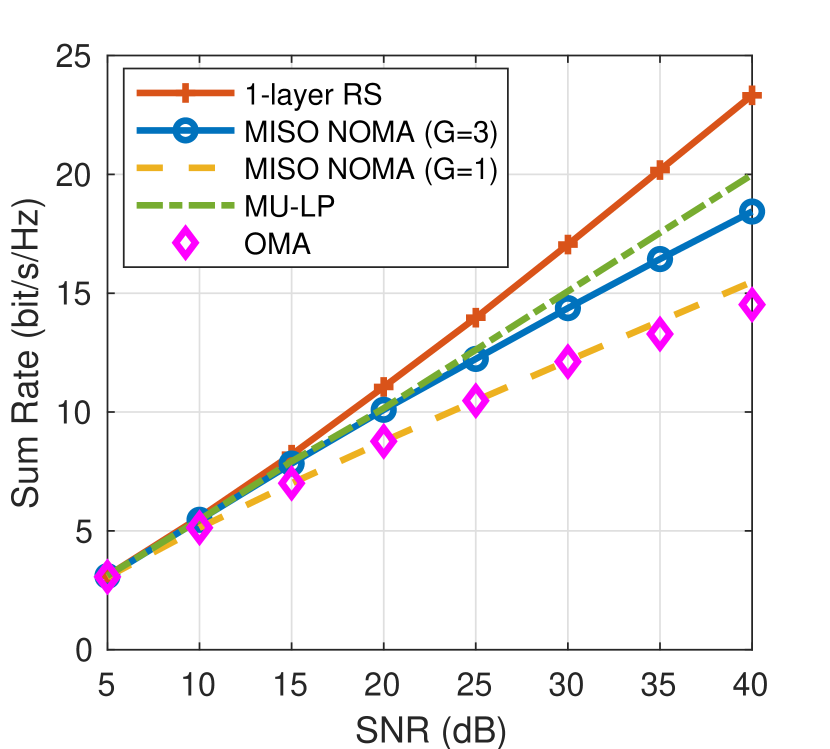
(a) $M=3$, $\sigma_{k}^{2}=1$

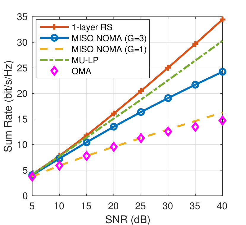
(b) $M=6,\sigma_{k}^{2}=1$

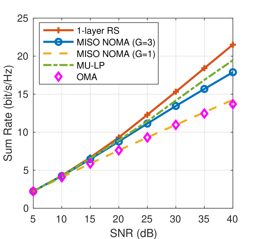
(c) $M=3,\sigma_{k}^{2}\in[0.1,1]$

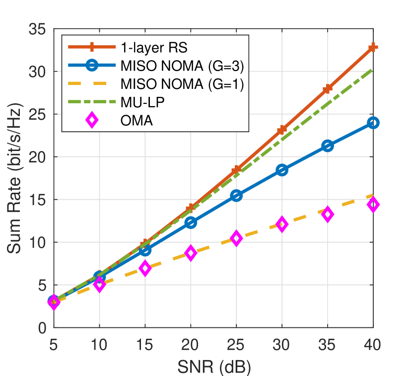
(d) $M=6,\sigma_{k}^{2}\in[0.1,1]$

Figure 13: Sum-rate vs. SNR comparison of different strategies with imperfect CSIT, $\alpha=0.5$, $K=6$.

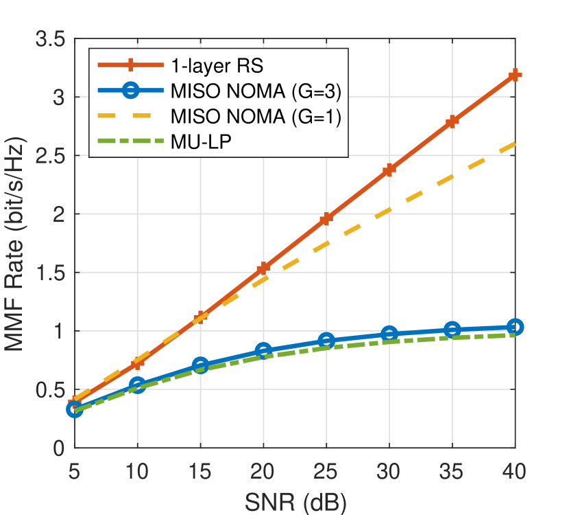
(a) $M=3$

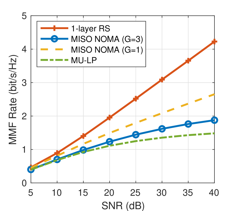
(b) $M=4$

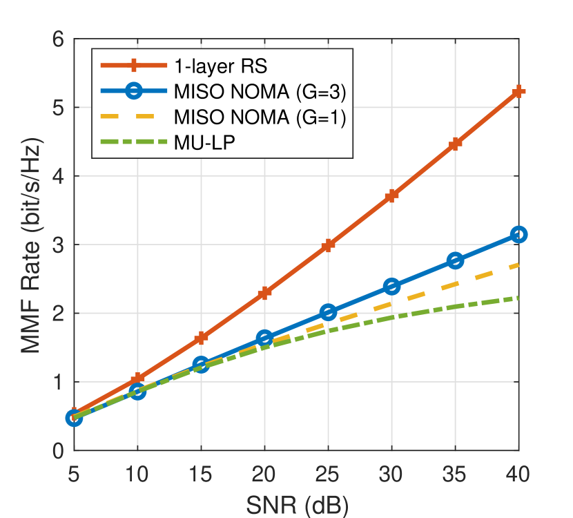
(c) $M=5$

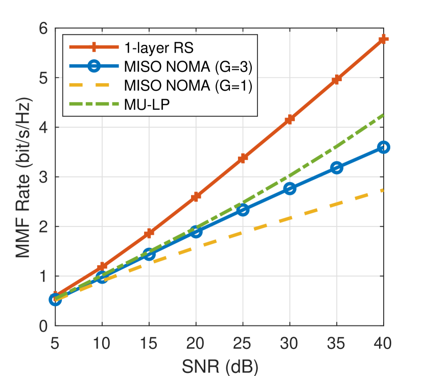
(d) $M=6$

Figure 14: Max-min rate vs. SNR comparison of different strategies with imperfect CSIT, $\alpha=0.5$, $K=6$, $\sigma_{k}^{2}=1,\forall k\in\mathcal{K}$.

Fig. 14 and 15 illustrate the MMF ergodic rate results. In general, the MMF multiplexing gains of all strategies in both figures match the theoretical MMF multiplexing gain results specified in Table II. When $M=3/4/5/6$, the corresponding MMF multiplexing gains of MISO NOMA ($G=3$) and MISO NOMA ($G=1$) when $\alpha=0.5$ are $d_{\textnormal{mmf}}^{(\textnormal{N,G=3})}=0/0/\frac{1}{4}/\frac{1}{4}$ and $d_{\textnormal{mmf}}^{(\textnormal{N,G=1})}=\frac{1}{6}/\frac{1}{6}/\frac{1}{6}/\frac{1}{6}$, respectively, and the corresponding MMF multiplexing gain of MU–LP and RS are $d_{\textnormal{mmf}}^{(\textnormal{M})}=0/0/0/\frac{1}{2}$, and $d_{\textnormal{mmf}}^{(\textnormal{R})}=\frac{1}{4}/\frac{1}{3}/\frac{1}{2}/\frac{1}{2}$. We observe that 1-layer RS achieves significantly higher multiplexing gains, which is also reflected in the MMF ergodic rate performance in Fig. 14 and 15. In both the perfect and imperfect CSIT settings, user fairness cannot be improved by MISO NOMA. The MMF ergodic rate performance of MISO NOMA is much worse than that of 1-layer RS.

Therefore, the four misconceptions behind multi-antenna NOMA are further verified for imperfect CSIT. Higher sum-rate and MMF rate gaps between RS and MU–LP/multi-antenna NOMA are generally observed by comparing the corresponding perfect and imperfect CSIT results. By partially decoding the interference and treating the remaining interference as noise, 1-layer RS is more robust to CSIT inaccuracy. The large performance gain of RS makes it an appealing strategy for future communication networks.

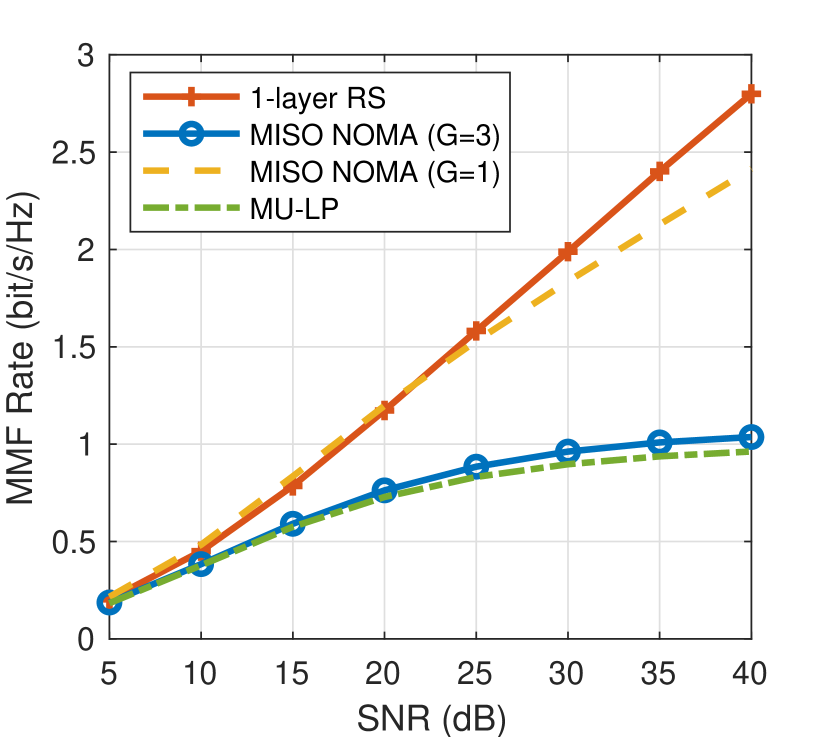
(a) $M=3$

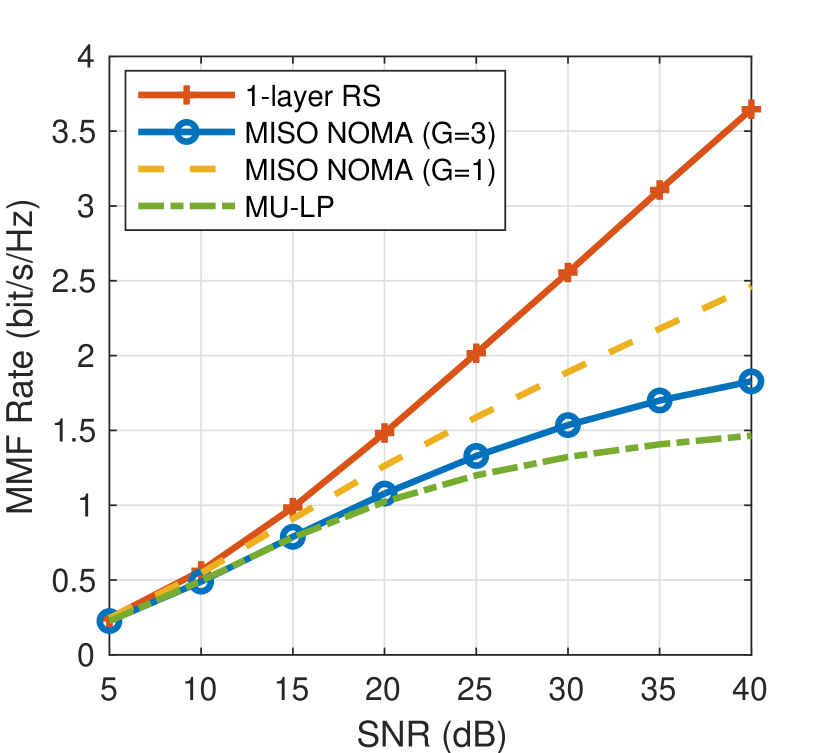
(b) $M=4$

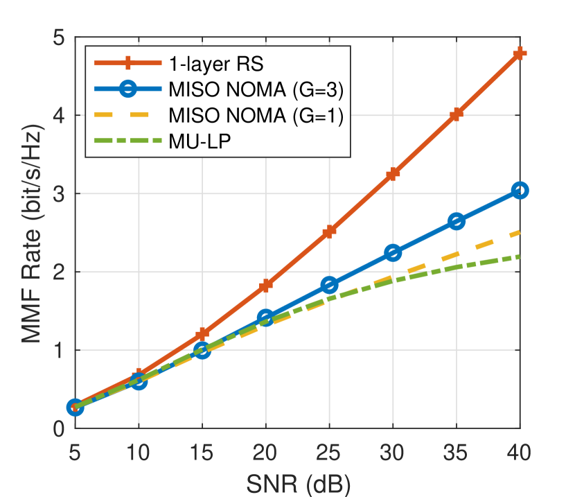
(c) $M=5$

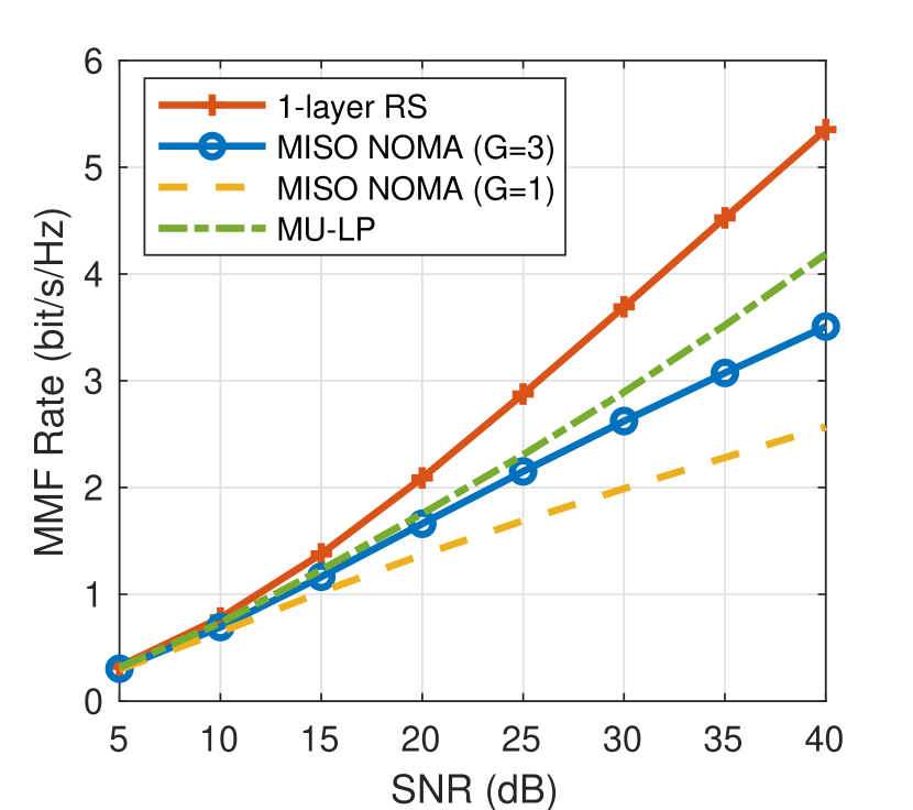
(d) $M=6$

Figure 15: Max-min rate vs. SNR comparison of different strategies with imperfect CSIT, $\alpha=0.5$, $K=6$, $\sigma_{k}^{2}\in[0.1,1],\forall k\in\mathcal{K}$.

VIII-C Discussions

The simulations so far fully validate the theoretical multiplexing gain analysis and confirm the inefficiency of MISO NOMA. We therefore conclude that the fundamental design principle of NOMA, namely forcing one user to decode the message(s) of other user(s), should be reconsidered or very carefully used for multi-antenna settings.

Thanks to its ability to partially decode interference and partially treat interference as noise, 1-layer RS achieves equal or higher sum-rate and MMF rate performance than all other strategies in both underloaded and overloaded regimes, especially when it comes to metrics that favor user fairness (e.g., MMF rate) in an overloaded regime. This is due to the fact that the inter-user interference becomes stronger in the setting when all users are active and the number of transmit antenna is limited. The superiority of 1-layer RS in managing multi-user interference becomes more pronounced when users suffer from stronger interference. Most importantly, 1-layer RS requires no user grouping and decoding order optimization at the transmitter and only one layer of SIC at each user. Compared with MISO NOMA, the sum-rate and MMF rate performance gain of RS comes at a much reduced transmitter and receiver complexity. 1-layer RS enables a better trade-off between the rate performance gains and the number of SIC layers. Hence, we conclude that 1-layer RS is a more powerful and promising strategy for multi-antenna networks.

Though the evaluations have been limited to 1-layer RS as the basic RSMA scheme, further rate enhancements over 1-layer RS can be obtained with multi-layer RS where the message of a user is split multiple times and multiple SIC layers are implemented at the receivers, as demonstrated in [47, 46, 68, 79, 80].

IX Conclusions and Future Research

This paper provides a broad, different and useful perspective on multi-antenna NOMA and non-orthogonal transmission to the community working on NOMA and multiple access, and to the future generations of researchers working on multi-user multi-antenna communications. Although NOMA in single-antenna settings has been well understood for a long time, the paper shows that the design of non-orthogonal transmission strategies for multi-antenna settings should be done with care so as to benefit from the multi-antenna dimensions and SIC receivers.

The paper showed in Section II that a two-user multi-antenna NOMA increases the receiver complexity and at the same time incurs a loss in multiplexing gain (and therefore rate at high SNR) compared to conventional multiuser precoding (as in used in 4G and 5G), therefore raising concerns on the efficiency of multi-antenna NOMA. Subsequently, a general $K$-user setting with perfect CSIT and imperfect CSIT were studied in Section III and Section IV, respectively and various multiplexing gains of multi-antenna NOMA were derived. Then we introduced two baseline schemes, namely $K$-user conventional multiuser precoding Section in V and $K$-user multi-antenna rate-splitting in Section VI, and studied the multiplexing gains of those schemes. Section VII compares the multiplexing gains of all considered schemes and provides strong theoretical grounds for performance comparisons among all schemes. In particular it identifies the scenarios where NOMA incurs a gain and a loss compared to multiuser linear precoding and demonstrates how NOMA always leads to lower multiplexing gains than rate-splitting though it makes use of a larger number of SIC layers at the receivers. This section is instrumental and exposes various misconceptions and shortcomings of multi-antenna NOMA. Simulation results are then used in Section VIII to confirm our findings and prediction from the multiplexing gain analysis.

Our results show that NOMA is not an efficient solution to cope with the high throughput, reliability, heterogeneity of Quality-of-Service (QoS), and connectivity requirements of the downlink of future 5G and beyond multi-antenna wireless networks. This is due to the fact that the fundamental principle of NOMA consisting in forcing one user in each group to fully decode the messages of other co-scheduled users is an inefficient design in multi-antenna settings. Consequently, the benefits to the research community and future standards and networks of multi-antenna NOMA for downlink communications (e.g. MISO/MIMO techniques for NOMA, NOMA for massive MIMO and cell-free massive MIMO, multi-antenna NOMA for millimetre and terahertz communications, NOMA for multi-beam satellite communications, multi-antenna NOMA in reconfigurable intelligent surfaces, multi-antenna in Multiuser Superposition Transmission (MUST) in 3GPP, etc) are questionable and should be considered carefully in light of the results in this paper.

Instead, non-orthogonal transmission strategies for multi-antenna settings should be designed such that interference is partially decoded and partially treated as noise based on the rate-splitting (multiple access) literature so as to truly benefit from multi-antenna transmitters (and potentially multi-antenna receivers) and SIC receivers.

In this paper, we limited the multiplexing gain analysis and the numerical evaluations to two metrics, namely sum multiplexing gain/sum-rate and MMF multiplexing gain/MMF rate, and to the MISO BC. Nevertheless, the results can be extended to other metrics such as the weighted sum-rate (WSR) and to other scenarios. Readers are invited to check [47] that confirms the inefficiency of NOMA and the superiority of RS from a WSR perspective, and are encouraged to consult the growing literature on RS (and RSMA) demonstrating the superiority of RS over NOMA and MU-LP in numerous scenarios and applications, namely multi-user multi-antenna communications [47, 67, 73], multigroup multicast [51, 36], energy efficiency [68, 74, 75], multi-cell joint transmission [76], non-orthogonal unicast and multicast transmission [68], wireless information and power transfer [77], cooperative communication with user relaying [78], imperfect CSIT [79, 80], link-level simulations [81], C-RAN [82], secrecy rate [83, 84], aerial networks [75, 85], imperfect CSIT and CSIR [86], visible light communications [87, 88], network performance analysis [89], reconfigurable intelligent surface [90].

The emphasis of the paper was on downlink multi-user communications. Results suggest that future downlink multi-user multi-antenna communications would strongly benefits from RSMA. RSMA is a gold mine of research problems for academia and industry with issues spanning numerous areas: RSMA to achieve the fundamental limits of wireless networks; RSMA for multi-user/multi-cell multi-antenna networks; RSMA-based robust interference management; RSMA in MU-MIMO, CoMP, Massive MIMO, millimetre wave and higher frequency bands, relay, cognitive radio, caching, physical layer security, cooperative communications, cloud-enabled platforms (C-RAN, F-RAN), intelligent reflecting surfaces, etc; RSMA to unify, generalize and outperform SDMA and NOMA; physical layer design of RSMA-based network; coding and Modulation for RSMA; cross-layer design, optimization and performance analysis of RSMA; implementation and standardization of RSMA; RSMA in B5G services such as enhanced eMBB, enhanced URLLC, enhanced MTC, massive MTC, massive IoT, V2X, cellular, UAV and satellite networks, wireless powered communications, integrated communications and sensing, etc. RSMA can also be used in the uplink, as originally shown for single-antenna systems in [91], and much is left to be done to identify the benefits of RSMA for general uplink multi-user multi-antenna communications. The performance benefits of RSMA vs NOMA vs OMA vs other multiple accesses in the uplink, beyond the existing NOMA vs OMA comparison [92], is also much worth investigating.

Appendix A Proof of Proposition 4

Let us first consider $G>1$ and $M\geq K-g+1$. Recalling from the proof of Proposition 3 that the sum multiplexing gain of $G\alpha$ can be split equally among the $G$ groups so that each group gets a (group) sum multiplexing gain of $\alpha$, and following again the MAC argument, the (group) sum multiplexing gain of $\alpha$ in each group can then be further split equally among the $g$ users, which leads to an upper bound on the MMF multiplexing gain of $\frac{\alpha}{g}$. Achievability is obtained by designing precoders using ZFBF, and allocating power (consider group 1 for simplicity) to user $k=1,\ldots,g$ as $O(P^{1-\frac{g-k}{g}\alpha})$, which causes the SINR for user-$k$ to scale as $O(P^{\alpha/g})$ and an achievable MMF multiplexing gain of $\frac{\alpha}{g}$.

To illustrate the achievability in more detail, we consider a simple example associated with $K=4$, $G=2$, $g=2$, and $M\geq 3$. First, we design the precoders $\mathbf{p}_{1}$ and $\mathbf{p}_{2}$ in group 1 to be orthogonal to the channel estimates $\hat{\mathbf{h}}_{3}$ and $\hat{\mathbf{h}}_{4}$ of users 3 and 4. Similarly, $\mathbf{p}_{3}$ and $\mathbf{p}_{4}$ in group 2 are made orthogonal to $\hat{\mathbf{h}}_{1}$ and $\hat{\mathbf{h}}_{2}$. Second, allocate power $O(P^{b})$ with $b=1-\alpha/2$ to users 1 and 3, and $O(P-P^{b})=O(P)$ to users 2 and 4. Using these precoders and power allocations, the received signals in group 1 can be written as

$$y_{1} =\underbrace{\mathbf{h}_{1}^{H}\mathbf{p}_{1}s_{1}}_{P^{b}}+\underbrace{\mathbf{h}_{1}^{H}\mathbf{p}_{2}s_{2}}_{P}+\underbrace{\tilde{\mathbf{h}}_{1}^{H}\mathbf{p}_{3}s_{3}}_{P^{b-\alpha}}+\underbrace{\tilde{\mathbf{h}}_{1}^{H}\mathbf{p}_{4}s_{4}}_{P^{1-\alpha}}+\underbrace{n_{1}}_{P^{0}},$$ (43)

$$y_{2} =\underbrace{\mathbf{h}_{2}^{H}\mathbf{p}_{1}s_{1}}_{P^{b}}+\underbrace{\mathbf{h}_{2}^{H}\mathbf{p}_{2}s_{2}}_{P}+\underbrace{\tilde{\mathbf{h}}_{2}^{H}\mathbf{p}_{3}s_{3}}_{P^{b-\alpha}}+\underbrace{\tilde{\mathbf{h}}_{2}^{H}\mathbf{p}_{4}s_{4}}_{P^{1-\alpha}}+\underbrace{n_{2}}_{P^{0}},$$ (44)

where the quantities under the brackets refer to how the power level of each term scales. From (43) and (44), $s_{2}$ can be decoded at an SINR level scaling as $\frac{P}{P^{b}+P^{1-\alpha}+P^{b-\alpha}+P^{0}}=\frac{P}{P^{b}}=P^{\alpha/2}$ (since $b\geq 1-\alpha\geq b-\alpha$ and $b\geq 0$). Using SIC, $s_{2}$ is cancelled in $\eqref{stream_1}$, and $s_{1}$ can be decoded at an SINR level scaling as $\frac{P^{b}}{P^{1-\alpha}+P^{b-\alpha}+P^{0}}=P^{\alpha/2}$. Similar expressions hold for group 2, and we note that all four streams have an SINR scaling as $P^{\alpha/2}$, therefore achieving an MMF multiplexing gain of $\frac{\alpha}{2}$.

Let us now consider $G>1$ and $M<K-g+1$. Since the MMF multiplexing gain collapses to 0 in the perfect CSIT setting, the same holds for imperfect CSIT.

Let us now consider $G=1$. The situation here is the same as in the perfect CSIT setting. There is no inter-group interference and the sum multiplexing gain of one in the single group can be split equally among the $K$ users, which leads to an upper bound on the MMF multiplexing gain of $\frac{1}{K}$. Achievability is obtained by choosing the powers of users $k=1,\ldots,K$ as $O(P^{k/K})$, which causes the SINR of user-$k$ to scale as $O(P^{1/K})$ and results in an achievable MMF multiplexing gain of $\frac{1}{K}$.

Appendix B WMMSE Optimization Framwork

The WMMSE optimization framework to solve both problems (41) and (42) is specified as follows.

At user-$j,j\in\mathcal{K}_{i}$, equalizer $g_{j,k}$ is employed to decode stream $s_{k},k\in\{k\mid k\geq j,k\in\mathcal{K}_{i}\}$. The estimate of $s_{k}$ at user-$j$ is obtained as $\widehat{s}_{j,k}=g_{j,k}y_{j,k}$, where $y_{j,k}=\sum_{m\leq k,m\in\mathcal{K}_{i}}\mathbf{h}_{j}^{H}\mathbf{p}_{m}s_{m}+\sum_{l\neq i,l\in\mathcal{G}}\sum_{m\in\mathcal{K}_{l}}\mathbf{h}_{j}^{H}\mathbf{p}_{m}s_{m}+n_{j}$ is the signal received at user-$j$ after removing the streams decoded before $s_{k}$. The corresponding Mean Square Error (MSE) is given by

$$\varepsilon_{j,k} =\mathbb{E}\{|\widehat{s}_{j,k}-s_{k}|^{2}\}$$ (45)

$$=|g_{j,k}|^{2}T_{j,k}-2\Re\{g_{j,k}\mathbf{h}_{j}^{H}\mathbf{p}_{k}\}+1,$$

where $T_{j,k}=|\mathbf{h}_{j}^{H}\mathbf{p}_{k}|^{2}+I_{j,k}^{(in)}+I_{j,k}^{(ou)}$ is the power received at user-$j$ when decoding $s_{k}$. Furthermore, $I_{j,k}^{(in)}$ and $I_{j,k}^{(ou)}$ are respectively the intra-group and inter-group interference power defined in (18).

By solving $\frac{\partial\varepsilon_{j,k}}{\partial g_{j,k}}=0$, the optimal Minimum MSE (MMSE) equalizer is calculated as

$$g_{j,k}^{\textrm{MMSE}}=\mathbf{p}_{k}^{H}\mathbf{h}_{j}({T}_{j,k})^{-1}.$$ (46)

Substituting (46) back to (45), the corresponding MMSE is then obtained as

$$\varepsilon_{j,k}^{\textrm{MMSE}}=\min_{g_{j,k}}\varepsilon_{j,k}=T_{j,k}^{-1}(I_{j,k}^{(in)}+I_{j,k}^{(ou)}).$$ (47)

With the introduced $\varepsilon_{j,k}^{\textrm{MMSE}}$, the rate at user-$j$ to decode the message of user-$k$ in (17) is equivalently written as $R_{j,k}=-\log_{2}(\varepsilon_{j,k}^{\textrm{MMSE}})$. Defining the Weighted MSE (WMSE) of $\varepsilon_{j,k}$ with a weight $u_{j,k}>0$ as

$$\xi_{j,k}=u_{j,k}\varepsilon_{j,k}-\log_{2}(u_{j,k}),$$ (48)

and defining its Weighted MMSE (WMMSE) by minimizing $\xi_{j,k}$ over $u_{j,k}$ and $g_{j,k}$ as

$$\xi_{j,k}^{\textrm{MMSE}}=\min_{u_{j,k},g_{j,k}}\xi_{j,k},$$ (49)

we then establish the rate-WMMSE relationship, which is given by

$$\xi_{j,k}^{\textrm{MMSE}}=1-R_{j,k}.$$ (50)

The rate-WMMSE relation in (50) is obtained as follows. The optimum equalizer is calculated as $g_{j,k}^{*}=g_{j,k}^{\textrm{MMSE}}$ from $\frac{\partial\xi_{j,k}}{\partial g_{j,k}}=0$. Substituting $g_{j,k}^{\textrm{MMSE}}$ back to (48) yields $\xi_{j,k}(g_{j,k}^{\textrm{MMSE}})=u_{j,k}\varepsilon_{j,k}^{\textrm{MMSE}}-\log_{2}(u_{j,k})$. By solving $\frac{\partial\xi_{j,k}(g_{j,k}^{\textrm{MMSE}})}{\partial g_{j,k}}=0$, we then obtain the optimal MMSE weight, which is given as

$$u_{j,k}^{*}=u_{j,k}^{\textrm{MMSE}}=(\varepsilon_{j,k}^{\textrm{MMSE}})^{-1}.$$ (51)

Substituting $u_{j,k}^{\textrm{MMSE}}$ back to $\xi_{j,k}(g_{j,k}^{\textrm{MMSE}})$, we have $\min_{u_{j,k},g_{j,k}}\xi_{j,k}=1-R_{j,k}$. Following (49), we obtain (50).

Motivated by the rate-WMMSE in (50), we find that the achievable rate of user-$k$ in (19) is equal to $R_{k}=1-\xi_{k}^{\textrm{MMSE}}$, where $\xi_{k}^{\textrm{MMSE}}=\max_{j\leq k,j\in\mathcal{K}_{i}}\xi_{j,k}^{\textrm{MMSE}}$. By defining the WMSE of user-$k$ as

$$\xi_{k}=\max_{j\leq k,j\in\mathcal{K}_{i}}\xi_{j,k},$$ (52)

and the respective set of equalizers and weights as $\mathbf{g}=\{g_{j,k}\mid j\leq k,k,j\in\mathcal{K}_{i},i\in\mathcal{G}\}$, $\mathbf{u}=\{u_{j,k}\mid j\leq k,k,j\in\mathcal{K}_{i},i\in\mathcal{G}\}$, the sum-rate WMMSE problem is formulated as

$$\min_{\mathbf{{P}},\mathbf{{u}},\mathbf{{g}}}\quad \sum_{k\in\mathcal{K}}\xi_{k}$$ (53a)

s.t. $$\text{tr}(\mathbf{P}\mathbf{P}^{H})\leq P.$$ (53b)

Following the proof of [43], we find that the MMSE solutions of the equalizers $\mathbf{g}^{\textrm{MMSE}}=\{g_{j,k}^{\textrm{MMSE}}\mid j\leq k,k,j\in\mathcal{K}_{i},i\in\mathcal{G}\}$ and weights $\mathbf{u}^{\textrm{MMSE}}=\{u_{j,k}^{\textrm{MMSE}}\mid j\leq k,k,j\in\mathcal{K}_{i},i\in\mathcal{G}\}$ satisfy the KKT optimality conditions of (53). Substituting ($\mathbf{g}^{\textrm{MMSE}},\mathbf{u}^{\textrm{MMSE}}$) back to (53) with affine transformations applied to the objective function, (53) boils down to (41). In fact, for any point ($\mathbf{{P}}^{*},\mathbf{{u}}^{*},\mathbf{{g}}^{*}$) satisfying the KKT optimality conditions of (53), the solution $\mathbf{{P}}^{*}$ satisfies the KKT optimality conditions of (41). Hence, (53) yields a solution for (41).

Although the transformed problem (53) is still non-convex, it is block-wise convex with respect to $\mathbf{{P}}$ and ($\mathbf{{g}},\mathbf{{u}}$). For a given $\mathbf{{P}}$, the optimal solution of the weights and equalizers are $\mathbf{g}^{\textrm{MMSE}}(\mathbf{{P}}),\mathbf{u}^{\textrm{MMSE}}(\mathbf{{P}})$. When ($\mathbf{{g}},\mathbf{{u}}$) are fixed, problem (53) becomes convex and can be solved by interior-point methods. Motivated by the block-wise convexity, we use the Alternating Optimization (AO) algorithm as illustrated in Algorithm 1 to solve (53). In each iteration, the equalizers and weights are first updated by ($\mathbf{g}^{\textrm{MMSE}}(\mathbf{{P}}),\mathbf{u}^{\textrm{MMSE}}(\mathbf{{P}})$) for a given $\mathbf{P}$. The updated equalizers and weights ($\mathbf{g}^{\textrm{MMSE}}(\mathbf{{P}}),\mathbf{u}^{\textrm{MMSE}}(\mathbf{{P}})$) are substituted back to (53). Precoder $\mathbf{{P}}$ is then updated by solving (53). $\mathbf{{P}}$ and ($\mathbf{{g}},\mathbf{{u}}$) are updated in an alternating manner until the convergence of the sum-rate. Algorithm 1 is guaranteed to converge and it converges to the KKT solution of problem (41). Readers are referred to [43] for the proof.

1 Initialize: $t\leftarrow 0$, $\mathbf{P}$;

2 repeat

3       $t\leftarrow t+1$, $\mathbf{P}^{[t-1]}\leftarrow\mathbf{P}$;

4       $\mathbf{g}\leftarrow\mathbf{g}^{\mathrm{MMSE}}(\mathbf{P}^{[t-1]})$; $\mathbf{u}\leftarrow\mathbf{u}^{\mathrm{MMSE}}(\mathbf{P}^{[t-1]})$;

5       Substitute $(\mathbf{g},\mathbf{u})$ back to (53) and update $\mathbf{P}$ by solving (53);

6until convergence;

Algorithm 1 AO algorithm

Following the same procedure, we are able to obtain the transformed WMMSE problem for max-min rate maximization, which is given by

$$\min_{\mathbf{{P}},\mathbf{{u}},\mathbf{{g}}}\quad \max_{k\in\mathcal{K}}\,\xi_{k}$$ (54a)

s.t. $$\text{tr}(\mathbf{P}\mathbf{P}^{H})\leq P.$$ (54b)

By substituting problem (53) in Algorithm 1 with problem (54), we obtain the corresponding AO Algorithm to achieve the KKT solution of the max-min rate problem (42).

References

- [1] Y. Saito, Y. Kishiyama, A. Benjebbour, T. Nakamura, A. Li, K. Higuchi, “Non-orthogonal multiple access (NOMA) for cellular future radio access,” Proc. IEEE 77th Veh. Technol. Conf. (VTC Spring), 2013
- [2] L. Dai, B Wang, Y Yuan, S Han, C-l I, Z Wang, “Non-orthogonal multiple access for 5G: solutions, challenges, opportunities, and future research trends,” IEEE Commun. Mag., vol. 53, no. 9, pp. 74–81, 2015.
- [3] Z. Ding, Y. Liu, J. Choi, Q. Sun, M Elkashlan, C-l I, H.V. Poor, “Application of non-orthogonal multiple access in LTE and 5G networks,” IEEE Commun. Mag., vol. 55, no. 2, pp. 185–191, 2017.
- [4] Y. Liu, Z. Qin, M. Elkashlan, Z. Ding, A. Nallanathan, and L. Hanzo, “Nonorthogonal multiple access for 5G and beyond,” Proceedings of the IEEE, Vol. 105, No. 12, Dec. 2017.
- [5] W. Shin, M. Vaezi, B. Lee, D.J. Love, J. Lee, H.V. Poor, “Non-orthogonal multiple access in multi-cell networks: theory, performance, and practical challenges,” IEEE Commun. Mag., vol. 55, no. 10, 176–183, Oct. 2017.
- [6] T. Cover, “Broadcast channels,” IEEE Trans. Inf. Theory., vol. 18, no. 1, pp. 2–14, 1972.
- [7] D. Tse, P. Viswanath, Fundamentals of wireless communication, Cambridge University Press, Cambridge, 2005.
- [8] A. Goldsmith, Wireless Communications, Cambridge University Press, Cambridge, 2005.
- [9] Q. Li, G. Li, W. Lee, M. Lee, D. Mazzarese, B. Clerckx, Z. Li, “MIMO techniques in WiMAX and LTE: a feature overview,” IEEE Communication Magazine, Vol.48, No.5, pp. 86-92, May 2010.
- [10] H. Weingarten, Y. Steinberg, S.S. Shamai, “The capacity region of the Gaussian multiple-input multiple-output broadcast channel,” IEEE Trans. Inf. Theory, vol. 52, no. 9, pp. 3936–3964, 2006.
- [11] Q. Spencer, A.L. Swindlehurst, and M. Haardt, “Zero-forcing methods for downlink spatial multiplexing in multi-user MIMO channels,” IEEE Trans. Signal Process., vol. 52, no. 2, pp. 462–471, February 2004.
- [12] M. Stojnic, H. Vikalo, and B. Hassibi, “Rate maximization in multiantenna broadcast channels with linear preprocessing,” IEEE Trans. Wireless Commun., vol. 5, no. 9, pp. 2338–2342, Sep. 2006.
- [13] A. D. Dabbagh and D. J. Love, “Precoding for multiple antenna gaussian broadcast channels with successive zero-forcing,” IEEE Trans. Signal Process., vol. 55, no. 7, pp. 3837-3850, July 2007.
- [14] A. D. Dabbagh and D. J. Love, “Multiple antenna MMSE based downlink precoding with quantized feedback or channel mismatch,” IEEE Trans. Commun., vol. 56, no. 11, pp. 1859-1868, Nov. 2008.
- [15] B. Clerckx, C. Oestges, MIMO wireless networks: channels, techniques and standards for multi-antenna, multi-user and multi-cell systems, Academic Press, Cambridge, 2013.
- [16] Y. Liu, H. Xing, C. Pan, A. Nallanathan, M. Elkashlan, L. Hanzo, “Multiple-antenna-assisted non-orthogonal multiple access,” IEEE Wireless Commun., vol. 25, no. 2, pp. 17–23, 2018.
- [17] M.F. Hanif, Z. Ding, T. Ratnarajah, G.K. Karagiannidis, “A minorization-maximization method for optimizing sum rate in the downlink of non-orthogonal multiple access systems,” IEEE Trans. Signal Process., vol. 64, no. 1, pp. 76–88, 2016.
- [18] J. Choi, “Minimum power multicast beamforming with superposition coding for multiresolution broadcast and application to NOMA systems,” IEEE Trans. Commun., vol. 63, no. 3, pp. 791–800, 2015.
- [19] Q. Sun, S. Han, C-l I, Z. Pan, “On the ergodic capacity of MIMO NOMA systems,” IEEE Wirel. Commun. Lett., vol. 4, no. 4, pp. 405–408, 2015.
- [20] Q. Zhang, Q. Li, J. Qin, “Robust beamforming for nonorthogonal multiple-access systems in MISO channels,” IEEE Trans. Veh. Technol., vol. 65, no. 12, pp. 10231–10236, 2016.
- [21] M. Zeng, A. Yadav, O. A. Dobre, G. I. Tsiropoulos, and H. V. Poor, “On the sum rate of MIMO-NOMA and MIMO-OMA systems,” IEEE Wireless Commun. Lett., Vol. 6, No. 4, Aug. 2017.
- [22] Z. Ding, R. Schober, and H. V. Poor, “A general MIMO framework for NOMA downlink and uplink transmission based on signal alignment,” IEEE Trans. Wireless Commun., vol. 15, no. 6, pp. 4438–4454, Jun. 2016
- [23] Z. Ding, F. Adachi, and H.V. Poor, “The application of MIMO to non-orthogonal multiple access,” IEEE Trans. Wirel. Commun., vol. 15, no. 1, pp. 537–552, 2016.
- [24] J. Choi, “On generalized downlink beamforming with NOMA,” J. Commun. Netw., vol. 19, no. 4, pp. 319–328, 2017.
- [25] W. Shin, M. Vaezi, B. Lee, D.J. Love, J. Lee, and H.V. Poor, “Coordinated beamforming for multi-cell MIMO-NOMA,” IEEE Commun. Lett., vol. 21, no. 1, pp. 84–87, 2017.
- [26] V.D. Nguyen, H.D. Tuan, T.Q. Duong, H.V. Poor, and O.S. Shin, “Precoder design for signal superposition in MIMO-NOMA multicell networks,” IEEE J. Sel. Areas Commun., vol. 35, no. 12, pp. 2681–2695, 2017.
- [27] M. Zeng, A. Yadav, O.A. Dobre, G.I. Tsiropoulos, and H.V. Poor, “Capacity comparison between MIMO-NOMA and MIMO-OMA with multiple users in a cluster,” IEEE J. Sel. Areas Commun., vol. 35, no. 10, pp. 2413–2424, 2017.
- [28] X. Chen, Z. Zhang, C. Zhong, and D. W. K. Ng, “Exploiting multiple antenna techniques for non-orthogonal multiple access,” IEEE J. Sel. Areas Commun., vol. 35, no. 10, pp. 2207-2220, Oct. 2017
- [29] F. Zhu, Z. Lu, J. Zhu, J. Wang, and Y. Huang, “Beamforming design for downlink non-orthogonal multiple access systems,” IEEE Access, vol. 6, pp. 10956–10965, 2018.
- [30] C. Chen, W. Cai, X. Cheng, L. Yang, and Y. Jin, “Low complexity beamforming and user selection schemes for 5G MIMO-NOMA systems,” IEEE J. Sel. Areas Commun., vol. 35, no. 12, pp. 2708–2722, Dec. 2017.
- [31] Y. Liu, M. Elkashlan, Z. Ding, and G. K. Karagiannidis, “Fairness of user clustering in MIMO non-orthogonal multiple access systems,” IEEE Commun. Lett., vol. 20, no. 7, pp. 1465-1468, Jul. 2016.
- [32] F. Alavi, K. Cumanan, Z. Ding, and A. G. Burr, “Beamforming techniques for nonorthogonal multiple access in 5G cellular networks,” IEEE Trans. Veh. Technol., vol. 67, no. 10, pp. 9474–9487, Oct. 2018.
- [33] Y. Jeong, C. Lee, and Y. H. Kim, “Power minimizing beamforming and power allocation for MISO-NOMA systems,” IEEE Trans. Veh. Technol., vol. 68, no. 6, pp. 6187–6191, Jun. 2019.
- [34] J. Zhang, Y. Zhu, S. Ma, X. Li, and K.-K. Wong, “Large system analysis of downlink MISO-NOMA system via regularized zero-forcing precoding With imperfect CSIT” IEEE Commun. Letters, vol. 24, no. 11, pp. 2454-2458, Nov. 2020.
- [35] Jianhang Chu, Xiaoming Chen, Caijun Zhong, and Zhaoyang Zhang, “Robust design for NOMA-based multi-Beam LEO satellite internet of things,” https://arxiv.org/abs/2008.03868.
- [36] A.Z. Yalcin, and M. Yuksel, “Max-min fair precoder design for non-orthogonal multiple access,” https://arxiv.org/abs/1911.09402.
- [37] Y. Liu, X. Mu, X. Liu, M. Di Renzo, Z. Ding, and R. Schober, “Reconfigurable intelligent surface (RIS) aided multi-user networks: interplay between NOMA and RIS,” arXiv:2011.13336.
- [38] Z. Chen, Z. Ding, P. Xu and X. Dai, “Optimal precoding for a QoS optimization problem in two-user MISO-NOMA downlink,” IEEE Commun. Lett., vol. 20, no. 6, pp. 1263-1266, June 2016
- [39] Z. Chen, Z. Ding, X. Dai and G. K. Karagiannidis, “On the application of quasi-degradation to MISO-NOMA downlink,” IEEE Trans. Signal Processing, vol. 64, no. 23, pp. 6174-6189, Dec., 2016
- [40] L. Dai, B. Wang, M. Peng and S. Chen, “Hybrid precoding-based millimeter-wave massive MIMO-NOMA with simultaneous wireless information and power transfer,” IEEE J. Sel. Areas Commun., vol. 37, no. 1, pp. 131-141, Jan. 2019.
- [41] B. Clerckx, H. Joudeh, C. Hao, M. Dai and B. Rassouli, “Rate splitting for MIMO wireless networks: A promising PHY-layer strategy for LTE evolution,” IEEE Commun. Mag., pp. 98-105, May 2016.
- [42] S. Yang, M. Kobayashi, D. Gesbert and X. Yi, “Degrees of Freedom of Time Correlated MISO Broadcast Channel With Delayed CSIT,” IEEE Trans. Inf. Theory, vol. 59, no. 1, pp. 315-328, Jan. 2013.
- [43] H. Joudeh et al., “Sum-rate maximization for linearly precoded downlink multiuser MISO systems with partial CSIT: A rate-splitting approach,” IEEE Trans. Commun., vol. 64, no. 11, pp. 4847-4861, Nov. 2016.
- [44] H. Joudeh and B. Clerckx, “Robust transmission in downlink multiuser MISO systems: A rate-splitting approach,” IEEE Trans. Signal Process., Vol. 64, No. 23, pp. 6227-6242, Dec. 2016.
- [45] C. Hao, Y. Wu, and B. Clerckx, “Rate analysis of two-receiver MISO broadcast channel with finite rate feedback: A rate-splitting approach,” IEEE Trans. Commun., vol. 63, no. 9, pp. 3232-3246, Sept. 2015.
- [46] M. Dai, B. Clerckx, D. Gesbert, and G. Caire, “A rate splitting strategy for massive MIMO with imperfect CSIT,” IEEE Trans. Wireless Commun., vol. 15, no. 7, pp. 4611-4624, July 2016.
- [47] Y. Mao, B. Clerckx, and V.O.K. Li, “Rate-splitting multiple access for downlink communication systems: bridging, generalizing and outperforming SDMA and NOMA,” EURASIP J. Wireless Commun. Netw., May 2018.
- [48] S. Timotheou and I. Krikidis, “Fairness for non-orthogonal multiple access in 5G systems,” IEEE Signal Process. Lett., vol. 22, no. 10, pp. 1647–1651, Oct. 2015.
- [49] J. Choi, “Power allocation for max-sum rate and max-min rate proportional fairness in NOMA,” IEEE Commun. Lett., vol. 20, no. 10, pp. 2055-2058, Oct. 2016.
- [50] L. Zheng and D. Tse, “Diversity and multiplexing: a fundamental tradeoff in multiple antenna channels,” IEEE Trans. Inf. Theory, vol. 49, no. 5, pp. 1073–1096, May 2003.
- [51] H. Joudeh and B. Clerckx, “Rate-splitting for max-min fair multigroup multicast beamforming in overloaded systems,” IEEE Trans. Wireless Commun., vol. 16, no. 11, pp. 7276-7289, Nov. 2017.
- [52] R. Knopp and P. A. Humblet, “Information capacity and power control in single-cell multiuser communications,” Proc. IEEE Int. Conf. Commun. (ICC), 1995.
- [53] G. Caire and S. Shamai (Shitz), “On the achievable throughput of a multiantenna Gaussian broadcast channel,” IEEE Trans. Inf. Theory, vol. 49, no. 7, pp. 1691–1706, Jul. 2003.
- [54] N. Jindal and A. Goldsmith, “Dirty-paper coding versus TDMA for MIMO broadcast channels,” IEEE Trans. Inf. Theory, vol. 51, no. 5, pp. 1783–1794, May 2005.
- [55] P. Ding, D. J. Love, and M. D. Zoltowski, “Multiple antenna broadcast channels with shape feedback and limited feedback,” IEEE Trans. Signal Process., vol. 55, no. 7, pp. 3417-3428, July 2007.
- [56] M. Kobayashi, N. Jindal and G. Caire,“Training and feedback optimization for multiuser MIMO downlink," IEEE Trans. on Commun., vol. 59, no. 8, pp. 2228-2240, August 2011.
- [57] H. V. Poor, “An Introduction to Signal Detection and Estimation,” Springer Science & Business Media, 2013.
- [58] A.G. Davoodi and S.A. Jafar, “Aligned image sets under channel uncertainty: Settling conjectures on the collapse of degrees of freedom under finite precision CSIT,” IEEE Trans. Inf. Theory, vol. 62, no. 10, pp. 5603–5618, Oct. 2016.
- [59] N. Jindal, “MIMO broadcast channels with finite-rate feedback,” IEEE Trans. Inf. Theory, vol. 52, no. 11, pp. 5045–5060, Nov. 2006.
- [60] L. Yin and B. Clerckx, “Rate-splitting multiple access for multigroup multicast and multibeam satellite systems,” IEEE Trans. on Commun., in press.
- [61] T. Han and K. Kobayashi, “A new achievable rate region for the interference channel,” IEEE Trans. Inf. Theory, vol. 27, no. 1, pp. 49–60, Jan. 1981.
- [62] E. Piovano and B. Clerckx, “Optimal DoF region of the K-user MISO BC with partial CSIT,” IEEE Commun. Lett., vol 21, no 11, pp 2368-2371, Nov 2017.
- [63] H. Joudeh and B. Clerckx, “DoF region of the MISO BC with partial CSIT: proof by inductive Fourier-Motzkin elimination,” Proc. IEEE Int. Workshop Signal Process. Adv. Wireless Commun. (SPAWC), 2019.
- [64] C. Hao, B. Rassouli, and B. Clerckx, “Achievable DoF regions of MIMO networks with imperfect CSIT,” IEEE Trans. on Inf. Theory, vol. 63, no. 10, pp. 6587-6606, Oct 2017.
- [65] A.G. Davoodi, and S. Jafar, “Degrees of freedom region of the (, , ) MIMO broadcast channel with partial CSIT: An application of sum-set inequalities based on aligned image sets,” IEEE Trans. Inf. Theory, in press.
- [66] K. Senel, H. V. Cheng , E. Bjornson, and E. G. Larsson, “What role can NOMA play in massive MIMO?” IEEE J. Sel. Topics in Signal Process., vol. 13, no. 3, pp. 597-611, June 2019.
- [67] B. Clerckx, Y. Mao, R. Schober, and H. V. Poor, “Rate-splitting unifying SDMA, OMA, NOMA, and multicasting in MISO broadcast channel: A simple two-user rate analysis,” IEEE Wireless Commun. Lett., vol. 9, no. 3, pp. 349–353, Mar. 2020.
- [68] Y. Mao, B. Clerckx and V.O.K. Li, “Rate-splitting for multi-antenna non-orthogonal unicast and multicast transmission: spectral and energy efficiency analysis,” IEEE Trans. on Commun., vol 67, no 12, pp. 8754-8770, Dec 2019.
- [69] M. Grant, S. Boyd, and Y. Ye. (2008), “CVX: MATLAB software for disciplined convex programming,” [Online]. Available: http://www.stanford.edu/ boyd/cvx
- [70] S.S. Christensen, R. Agarwal, E.D. Carvalho, and J.M. Cioffi, “Weighted sum-rate maximization using weighted MMSE for MIMO-BC beamforming design,” IEEE Trans. Wireless Commun., vol. 7, no. 12, pp. 4792–4799, Dec 2008.
- [71] 3GPP TR 36.931 “LTE; Evolved universal terrestrial aadio access (E-UTRA); radio frequency (RF) requirements for LTE pico node B," May 2011.
- [72] A. Shapiro, D. Dentcheva, and A. Ruszczyński. “Lectures on Stochastic Programming: Modeling and Theory," Society for Industrial and Applied Mathematics, 2014.
- [73] Z. Yang, M. Chen, W. Saad, and M. Shikh-Bahaei, “Optimization of rate allocation and power control for rate splitting multiple access (RSMA),” https://arxiv.org/abs/1903.08068
- [74] Y. Mao, B. Clerckx and V.O.K. Li, “Energy efficiency of rate-splitting multiple access, and performance benefits over SDMA and NOMA,” Proc. IEEE Int. Symp. Wireless Commun. Syst. (ISWCS) 2018.
- [75] A. Rahmati, Y. Yapici, N. Rupasinghe, I. Guvenc, H. Dai, and A. Bhuyan, “Energy efficiency of RSMA and NOMA in cellular connected mmWave UAV networks,” Proc. IEEE Int. Conf. Commun. (ICC), 2019
- [76] Y. Mao, B. Clerckx and V.O.K. Li, “Rate-splitting multiple access for coordinated multi-point joint transmission,” Proc. IEEE Int. Conf. Commun. (ICC), 2019
- [77] Y. Mao, B. Clerckx, V.O.K. Li, “Rate-splitting for multi-user multi-antenna wireless information and power transfer,” Proc. IEEE Int. Workshop Signal Process. Adv. Wireless Commun. (SPAWC), 2019
- [78] J. Zhang, B. Clerckx, J. Ge, and Y. Mao, “Cooperative rate-splitting for MISO broadcast channel with user relaying, and performance benefits over cooperative NOMA” IEEE Signal Processing Letters, vol. 26, no. 11, pp. 1678-1682, Nov 2019.
- [79] Y. Mao and B. Clerckx, “Beyond dirty paper coding for multi-antenna broadcast channel with partial CSIT: A rate-splitting approach,” IEEE Trans. on Commun., vol 68, no. 11, pp. 6775-6791, Nov. 2020.
- [80] Y. Mao, and B. Clerckx, “Dirty Paper Coded Rate-Splitting for Non-orthogonal Unicast and Multicast Transmission with Partial CSIT,” Asilomar Conference on Signals, Systems, and Computers 2020.
- [81] O. Dizdar, Y. Mao, W. Han, and B. Clerckx, “Rate-splitting multiple access for downlink multi-antenna communications: physical layer design and link-level simulations,” Proc. IEEE Annu. Symp. Pers. Indoor Mobile Radio Commun. (PIMRC), 2020.
- [82] D. Yu, J. Kim, and S. Park, “An efficient rate-splitting multiple access scheme for the downlink of C-RAN systems,” IEEE Wireless Commun. Lett., vol. 8, no. 6, pp. 1555-1558, Dec 2019.
- [83] P. Li, M. Chen, Y. Mao, Z. Yang, B. Clerckx, and M. Shikh-Bahaei, “Cooperative rate-splitting for secrecy sum-rate enhancement in multi-antenna broadcast channels,” Proc. IEEE Annu. Symp. Pers. Indoor Mobile Radio Commun. (PIMRC), 2020.
- [84] H. Fu, S. Feng, W. Tang, D.W.K. Ng “Robust secure resource allocation for downlink two-user MISO rate-splitting systems,” Proc. IEEE Int. Conf. Commun. (ICC), 2020.
- [85] W. Jaafar, S. Naser, S. Muhaidat, P.C. Sofotasios, Halim Yanikomeroglu, “Multiple access in aerial networks: from orthogonal and non-orthogonal to rate-splitting,” arXiv:2005.13122.
- [86] J. An, O. Dizdar, B. Clerckx, and W. Shin, “Rate-splitting multiple Access for multi-antenna broadcast channel with imperfect CSIT and CSIR,” Proc. IEEE Annu. Symp. Pers. Indoor Mobile Radio Commun. (PIMRC), 2020.
- [87] S. Tao, H.-Y. Yu, L. Qing, Y. Tang, D. Zhang, “One-layer rate-splitting multiple access with benefits over power-domain NOMA in indoor multi-cell VLC networks,” Proc. IEEE Int. Conf. Commun. (ICC), 2020.
- [88] S. Naser, L. Bariah, W. Jaafar, S. Muhaidat, P.C. Sofotasios, M. Al-Qutayri, O.A. Dobre, “Rate-splitting multiple access: unifying NOMA and SDMA in MISO VLC Channels,” https://arxiv.org/abs/2007.13560
- [89] E. Demarchou, C. Psomas, I. Krikidis, “Channel statistics-based rate splitting with spatial randomness,” Proc. IEEE Int. Conf. Commun. (ICC), 2020.
- [90] Z. Yang, J. Shi, Z. Li, M. Chen, W. Xu, M. Shikh-Bahaei, “Energy efficient rate splitting multiple access (RSMA) with reconfigurable intelligent surface,” Proc. IEEE Int. Conf. Commun. (ICC), 2020.
- [91] B. Rimoldi and R. Urbanke, “A rate-splitting approach to the Gaussian multiple-access channel,” IEEE Trans. Inf. Theory, vol. 42, no. 2, pp. 364-375, Mar. 1996.
- [92] Z. Wei, L. Yang, D.W.K. Ng, J. Yuan, and L. Hanzo, “On the performance gain of NOMA over OMA in uplink communication systems,” IEEE Trans. Commun., vol. 68, no. 1, pp. 536-568, Jan. 2020.