Full-Information Estimation of Heterogeneous Agent Models Using Macro and Micro Data

Abstract:

We develop a generally applicable full-information inference method for heterogeneous agent models, combining aggregate time series data and repeated cross sections of micro data. To handle unobserved aggregate state variables that affect cross-sectional distributions, we compute a numerically unbiased estimate of the model-implied likelihood function. Employing the likelihood estimate in a Markov Chain Monte Carlo algorithm, we obtain fully efficient and valid Bayesian inference. Evaluation of the micro part of the likelihood lends itself naturally to parallel computing. Numerical illustrations in models with heterogeneous households or firms demonstrate that the proposed full-information method substantially sharpens inference relative to using only macro data, and for some parameters micro data is essential for identification.

Keywords: Bayesian inference, data combination, heterogeneous agent models
JEL codes: C11, C32, E1

1 Introduction

Macroeconomic models with heterogeneous agents have exploded in popularity in recent years. New micro data sets – including firm and household surveys, social security and tax records, and censuses – have exposed the empirical failures of traditional representative agent approaches. The new models not only improve the fit to the data, but also make it possible to meaningfully investigate the causes and consequences of inequality among households or firms along several dimensions, including endowments, financial constraints, age, size, location, etc.

So far, however, empirical work in this area has only been able to exploit limited features of the micro data sources that motivated the development of the new models. As emphasized by Ahn, Kaplan, Moll, Winberry, and Wolf (2017), the burgeoning academic literature has mostly calibrated model parameters and performed over-identification tests by matching a few empirical moments that are deemed important a priori. This approach may be highly inefficient, as it ignores that the models’ implied macro dynamics and cross-sectional properties often fully determine the entire distribution of the observed macro and micro data. The failure to exploit the joint information content of macro and micro data stands in stark contrast to the well-developed inference procedures for estimating representative agent models using only macro data (Herbst and Schorfheide, 2016).

To exploit the full information content of macro and micro data, we develop a general technique to perform Bayesian inference in heterogeneous agent models. We assume the availability of aggregate time series data as well as repeated cross sections of micro data. Evaluation of the joint macro and micro likelihood function is complicated by the fact that the model-implied cross-sectional distributions typically depend on unobserved aggregate state variables. To overcome this problem, we devise a way to compute a numerically unbiased estimate of the model-implied likelihood function of the macro and micro data. As argued by Andrieu, Doucet, and Holenstein (2010) and Flury and Shephard (2011), such an unbiased likelihood estimate can be employed in standard Markov Chain Monte Carlo (MCMC) procedures to generate draws from the fully efficient Bayesian posterior distribution given all available data.

The starting point of our analysis is the insight that existing solution methods for heterogeneous agent models directly imply the functional form of the joint sampling distribution of macro and micro data, given structural parameters. These models are typically solved numerically by imposing a flexible functional form on the relevant cross-sectional distributions (e.g., a discrete histogram or parametric family of densities). The distributions are governed by time-varying unobserved state variables (e.g., moments). To calculate the model-implied likelihood, we decompose it into two parts. First, heterogeneous agent models are typically solved using the method of Reiter (2009), which linearizes with respect to the macro shocks but not the micro shocks. Hence, the macro part of the likelihood can be evaluated using standard linear state space methods, as proposed by Mongey and Williams (2017) and Winberry (2018). Second, the likelihood of the repeated cross sections of micro data, conditional on the macro state variables, can be evaluated by simply plugging into the assumed cross-sectional density. The key challenge that our method overcomes is that the econometrician typically does not directly observe the macro state variables. Instead, the observed macro time series are imperfectly informative about the underlying states.

Our procedure can loosely be viewed as a rigorous Bayesian version of a two-step approach: First we estimate the latent macro states from macro data, and then we compute the model-implied cross-sectional likelihood conditional on these estimated macro states. More precisely, we obtain a numerically unbiased estimate of the likelihood by averaging the cross-sectional likelihood across repeated draws from the smoothing distribution of the hidden states given the macro data. We emphasize that, despite being based on a likelihood estimate, our method is fully Bayesian and automatically takes into account all sources of uncertainty about parameters and states. An attractive computational feature is that evaluation of the micro part of the likelihood lends itself naturally to parallel computing. Hence, computation time scales well with the size of the data set. Though our baseline method is designed for repeated cross sections of micro data, we present ideas for exploiting panel data in Section 6.

We perform finite-sample valid and fully efficient Bayesian inference by plugging the unbiased likelihood estimate into a standard MCMC algorithm. The generic arguments of Andrieu, Doucet, and Holenstein (2010) and Flury and Shephard (2011) imply that the ergodic distribution of the MCMC chain is the full-information posterior distribution that we would have obtained if we had known how to evaluate the exact likelihood function (not just an unbiased estimate of it). This is true no matter how many smoothing draws are used to compute the unbiased likelihood estimate. In principle, we may use any MCMC posterior sampling algorithm that relies only on evaluating (the unbiased estimate of) the posterior density, such as Random Walk Metropolis-Hastings.

In contrast to other estimation methods, our full-information method is automatically finite-sample efficient and can easily handle unobserved individual heterogeneity, micro measurement error, as well as data imperfections such as selection or censoring. In an important early work, Mongey and Williams (2017) propose to exploit micro data by collapsing it to time series of cross-sectional moments and incorporating these into the macro likelihood. In principle, this approach can be as efficient as our full-information approach if the structural model implies that these moments are sufficient statistics for the micro data. We provide examples where this is not the case, for example due to the presence of unobserved individual heterogeneity and/or micro measurement error. Even when sufficient statistics do exist, it is necessary to properly account for sampling error in the observed cross-sectional moments, which is done automatically by our full-information likelihood method, but could be delicate and imprecise for moment-based approaches. Moreover, textbook adjustments to the micro likelihood allow us to accommodate specific empirically realistic features of micro data such as selection (e.g., over-sampling of large firms) or censoring (e.g., top-coding of income), whereas this is challenging to do efficiently with moment-based approaches.

We illustrate the joint inferential power of macro and micro data through two numerical examples: a heterogeneous household model (Krusell and Smith, 1998) and a heterogeneous firm model (Khan and Thomas, 2008). In both cases we assume that the econometrician observes certain standard macro time series as well as intermittent repeated cross sections of, respectively, (i) household employment and income and (ii) firm capital and labor inputs. Using simulated data, and given flat priors, we show that our full-information method accurately recovers the true structural model parameters. Importantly, for several structural parameters, the micro data reduces the length of posterior credible intervals substantially, relative to inference that exploits only the macro data. In fact, we give examples of parameters that can only be identified if micro data is available. In contrast, inference from moment-based approaches can be highly inaccurate and sensitive to the choice of moments.

We deliberately keep our numerical illustrations low-dimensional and build our code on top of the user-friendly Dynare-based model solution method of Winberry (2018). Though pedagogically useful, this particular numerical model solution method cannot handle very rich models, so a full-scale empirical illustration is outside the scope of this paper. However, there is nothing in our general inference approach that rules out larger-scale models. We argue in Section 7 that our general inference approach is compatible with cutting-edge model solution methods that apply automatic dimension reduction of the state space equations (Ahn, Kaplan, Moll, Winberry, and Wolf, 2017).

Literature.

Our paper contributes to the recent literature on structural estimation of heterogeneous agent models by exploiting the full, combined information content available in macro and micro data. We build on the idea of Mongey and Williams (2017) and Winberry (2018) to estimate heterogeneous agent models from the linear state space representation obtained from the Reiter (2009) model solution approach. Several papers have exploited only macro data (as well as calibrated steady-state micro moments) for estimation, including Winberry (2018), Hasumi and Iiboshi (2019), Acharya, Negro, and Dogra (2020), Auclert, Rognlie, and Straub (2020), and Auclert, Bardóczy, Rognlie, and Straub (2021). Challe, Matheron, Ragot, and Rubio-Ramirez (2017), Mongey and Williams (2017), Bayer, Born, and Luetticke (2020), and Papp and Reiter (2020) additionally track particular cross-sectional moments over time. In contrast, we exploit the entire model-implied likelihood function given repeated micro cross sections, which is (at least weakly) more efficient, as discussed further in Section 3.3.

We are not aware of other papers that tackle the fundamental problem that the aggregate shocks affecting cross-sectional heterogeneity are not directly observed. Parra-Alvarez, Posch, and Wang (2020) use the model-implied steady-state micro likelihood in a heterogeneous household model, but abstract from macro data or aggregate dynamics. Closest to our approach are Fernández-Villaverde, Hurtado, and Nuño (2019), who exploit the model-implied joint sampling density of macro and micro data in a particular heterogeneous agent macro model. However, they assume that the underlying state variables are directly observed, whereas our contribution is to solve the computational challenges that arise in the generic case where the macro states are (partially) latent.

Certain other existing methods for combining macro and micro data cannot be applied in our setting. Hahn, Kuersteiner, and Mazzocco (2022) develop asymptotic theory for estimation using interdependent micro and macro data sets, but their full-information approach requires derivatives of the exact likelihood in closed form, which is not available in our setting due to the need to integrate out unobserved state variables. Chang, Chen, and Schorfheide (2021) propose a reduced-form approach to estimating the feedback loop between aggregate time series and heterogeneous micro data; they do not consider estimation of structural models. In likelihood estimation of representative agent models, micro data has mainly been used to inform the prior, as in Chang, Gomes, and Schorfheide (2002). Finally, unlike the microeconometric literature on heterogeneous agent models (Arellano and Bonhomme, 2017), our work explicitly seeks to estimate the deep parameters of a general equilibrium macro model by also incorporating aggregate time series data.

Outline.

Section 2 shows that heterogeneous agent models imply a fully-specified statistical model for the macro and micro data. Section 3 presents our method for computing an unbiased likelihood estimate that is used to perform efficient Bayesian inference. There we also compare our full-information approach with moment-based estimation approaches. Sections 4 and 5 illustrate the inferential power of combining macro and micro data using two simple numerical examples, a heterogeneous household model and a heterogeneous firm model. Section 6 proposes an extension to panel data. Section 7 concludes and discusses possible future research directions. Appendix A contains proofs and technical results. A Supplemental Appendix and a full Matlab code suite are available online.

2 Framework

We first describe how heterogeneous agent models generically imply a statistical model for the macro and micro data. Then we illustrate how a simple model with heterogeneous households fits into this framework.

2.1 A general heterogeneous agent framework

Consider a given structural model that implies a fully-specified equilibrium relationship among a set of aggregate and idiosyncratic variables. We assume the availability of macro time series data as well as repeated cross sections of micro data, as summarized in Figure 1. Let $\mathbf{x}\equiv\{x_{t}\}_{1\leq t\leq T}$ denote the vector of observed time series data (e.g., real GDP growth), where $x_{t}$ is a vector, and $T$ denotes the time series sample size. At a subset $\mathcal{T}\subset\{1,2,\dots,T\}$ of time points we additionally observe the micro data $\mathbf{y}\equiv\{y_{i,t}\}_{1\leq i\leq N_{t},t\in\mathcal{T}}$, where $y_{i,t}$ is a vector (e.g., the asset holdings of household $i$ or the employment of firm $i$). At each time $t$, the cross section $\{y_{i,t}\}_{1\leq i\leq N_{t}}$ is sampled at random from the model-implied cross-sectional distribution conditional on some macro state vector $z_{t}$. For now it is convenient to assume that $\{y_{i,t}\}$ constitutes a representative sample, but sample selection or censoring are easily accommodated in the framework, as we demonstrate in Section 5.4. Formally, we make the following assumption.

Assumption 1.

The data is sampled as follows:

1. Conditional on $\mathbf{z}\equiv\{z_{t}\}_{t=1}^{T}$, the micro data $\{y_{i,t}\}_{1\leq i\leq N_{t},t\in\mathcal{T}}$ is independent across $t$ and the data points $\{y_{i,t}\}_{i=1}^{N_{t}}$ at time $t$ are sampled i.i.d. from the density $p(y_{i,t}\mid z_{t},\theta)$.

2. Conditional on $\mathbf{z}$, the micro data $\mathbf{y}$ is independent of the macro data $\mathbf{x}$.

3. Conditional on $z_{t}$ and $\{x_{\tau},z_{\tau}\}_{\tau\leq t-1}$, the macro data $x_{t}$ is sampled from the density $p(x_{t}\mid z_{t},\theta)$. Conditional on $\{z_{\tau}\}_{\tau\leq t-1}$, the state vector $z_{t}$ is sampled from the density $p(z_{t}\mid z_{t-1},\theta)$.

The first condition above operationalizes the notion of representative sampling of repeated cross sections. The second condition entails no loss of generality, since we can always include $x_{t}$ in the state vector $z_{t}$. The third condition is a standard Markovian state space formulation of the aggregate dynamics, as discussed further below.

Figure 1: Diagram of the distribution of the macro and micro data implied by a heterogeneous agent model. The state vector $z_{t}$ includes any time-varying parameters that govern the cross-sectional distribution $p(y_{i,t}\mid z_{t},\theta)$.

Given the structural parameter vector $\theta$, the fully-specified heterogeneous agent model implies functional forms for the macro observation density $p(x_{t}\mid z_{t},\theta)$, the macro state transition density $p(z_{t}\mid z_{t-1},\theta)$, and the micro sampling density $p(y_{i,t}\mid z_{t},\theta)$. These density functions reflect the equilibrium of the model, as we illustrate in the next subsection, and they are the key inputs in the likelihood computation in Section 3. Notice that the framework allows the micro and macro data to be dependent, though this dependence must be fully captured by the macro state vector $z_{t}$, which is determined by the structure of the model at hand. Because the sampling densities $p(x_{t}\mid z_{t},\theta)$ and $p(y_{i,t}\mid z_{t},\theta)$ are derived from an equilibrium model, the likelihood function derived below in equation (5) automatically embodies any constraints of the type envisioned by Imbens and Lancaster (1994) on the relationship between the aggregate macro data and the time-varying population moments of the micro sampling distribution. For example, if $y_{i,t}$ equals individual-level consumption, $x_{t}$ equals aggregate consumption, and $z_{t}$ equals the underlying macro shocks (which determine the dynamics of aggregates and of the micro distribution), then the asymptotic adding-up constraint that $\lim_{N_{t}\to\infty}\frac{1}{N_{t}}\sum_{i=1}^{N_{t}}y_{i,t}\stackrel{{\scriptstyle a.s.}}{{=}}x_{t}$ will be automatically satisfied if the sampling densities are derived from a model that imposes market clearing.

In most applications, some of the aggregate state variables $z_{t}$ that influence the macro and micro sampling densities are unobserved, i.e., $z_{t}\neq x_{t}$. This fact complicates the evaluation of the exact likelihood function and is the key technical challenge that we overcome in this paper, as discussed in Section 3.

2.2 Example: Heterogeneous household model

We use a simple heterogeneous household model à la Krusell and Smith (1998) to illustrate the components of the general framework introduced in Section 2.1. Our discussion of the model and the numerical equilibrium solution technique largely follows Winberry (2016, 2018). Though this model is far too stylized for quantitative empirical work, we demonstrate the flexibility of our framework by adding complications such as permanent heterogeneity among households as well as measurement error in observables. In Section 4 we will estimate a calibrated version of this model on simulated data.

Model assumptions.

A continuum of heterogeneous households $i\in[0,1]$ are exposed to idiosyncratic employment risk as well as aggregate shocks to wages and asset returns. Households have log preferences over consumption $c_{i,t}$ at time $t=0,1,2,\dots$. When employed ($\epsilon_{i,t}=1$), households receive wage income net of an income tax levied at rate $\tau$. When unemployed ($\epsilon_{i,t}=0$), they receive unemployment benefits equal to a fraction $b$ of their hypothetical working wage. The idiosyncratic unemployment state $\epsilon_{i,t}$ evolves exogenously according to a two-state first-order Markov process that is independent of aggregate conditions and household decisions. Households cannot insure themselves against their employment risk, since the only available financial instruments are shares of capital $\tilde{a}_{i,t}$, which yield a rate of return $r_{t}$. Financial investment is subject to the borrowing constraint $\tilde{a}_{i,t}\geq 0$.

For expositional purposes, we add a dimension of permanent household heterogeneity: Each household is endowed with a permanent labor productivity level $\lambda_{i}$, which is drawn at the beginning of time from a lognormal distribution with mean parameter $\mathbb{E}[\log\lambda_{i}]=\mu_{\lambda}\leq 0$ and variance parameter chosen such that $\mathbb{E}[\lambda_{i}]=1$. An employed household inelastically supplies $\lambda_{i}$ efficiency units of labor, earning pre-tax income of $\lambda_{i}w_{t}$, where $w_{t}$ is the real wage per efficiency unit of labor.

To summarize, the households’ problem can be written

$$\max_{c_{i,t},a_{i,t}\geq 0}\mathbb{E}_{0}\left[\sum_{t=0}^{\infty}\beta^{t}\log c_{i,t}\right]$$

$$\;\text{s.t.}\quad c_{i,t}=\lambda_{i}\big{\{}w_{t}[(1-\tau)\epsilon_{i,t}+b(1-\epsilon_{i,t})]+(1+r_{t})a_{i,t-1}-a_{i,t}\big{\}},$$

where $a_{i,t}=\tilde{a}_{i,t}/\lambda_{i}$ are the normalized asset holdings.

A representative firm produces the consumption good using a Cobb-Douglas production function $Y_{t}=e^{\zeta_{t}}K_{t}^{\alpha}L^{1-\alpha}$, where aggregate capital $K_{t}$ depreciates at rate $\delta$, and $L$ is the aggregate level of labor efficiency units (which is constant over time since employment risk is purely idiosyncratic). The firm hires labor and rents capital in competitive input markets. Log total factor productivity (TFP) evolves as an AR(1) process $\zeta_{t}=\rho_{\zeta}\zeta_{t-1}+\varepsilon_{t}$, where $\varepsilon_{t}\overset{i.i.d.}{\sim}N(0,\sigma_{\zeta}^{2})$. The government balances its budget period by period, implying $\tau L=b(1-L)$.

We collect the deep parameters of this model in the vector $\theta$. These include $\beta$, $\alpha$, $\delta$, $\tau$, $\rho_{\zeta}$, $\sigma_{\zeta}$, the transition probabilities for idiosyncratic employment states, and $\mu_{\lambda}$.

Equilibrium definition and computation.

The mathematical definition of a recursive competitive equilibrium is standard, and we refer to Winberry (2016) for details. We now review Winberry’s method for solving the model numerically.

A key model object is the cross-sectional joint distribution of the micro state variables, i.e., employment status $\epsilon_{i,t}$, normalized assets $a_{i,t-1}$, and permanent productivity $\lambda_{i}$. This distribution, which we denote $\tilde{\mu}_{t}(\epsilon,a,\lambda)$, is time-varying as it implicitly depends on the aggregate productivity state variable $\zeta_{t}$ at time $t$. Due to log utility and the linearity of the households’ budget constraint in $\lambda_{i}$, macro aggregates are unaffected by the distribution of the permanent cross-sectional heterogeneity $\lambda_{i}$ (recall that $\mathbb{E}[\lambda_{i}]=1$). This implies that the mean parameter $\mu_{\lambda}$ of the log-normal distribution of $\lambda_{i}$ is only identifiable if micro data is available, as discussed further in Section 4. In equilibrium we have $\tilde{\mu}_{t}(\epsilon,a,\lambda)=\mu_{t}(\epsilon,a)F(\lambda\mid\mu_{\lambda})$, where $F(\cdot\mid\mu_{\lambda})$ denotes the time-invariant log-normal distribution for $\lambda_{i}$.

To solve the model numerically, Winberry (2016, 2018) assumes that the infinite-dimensional cross-sectional distribution $\mu_{t}(\epsilon,a)$ can be well approximated by a rich but finite-dimensional family of distributions. The distribution of $a$ given $\epsilon$ is a mixture of a mass point at 0 (the borrowing constraint) and an absolutely continuous distribution concentrated on $(0,\infty)$. At every point in time, Winberry approximates the absolutely continuous part using a density of the exponential form

$$g_{\epsilon}(a)=\exp\left\{\tilde{\varphi}_{\epsilon 0}+\tilde{\varphi}_{\epsilon 1}\tilde{m}_{\epsilon 1}+\sum_{\ell=2}^{q}\varphi_{\epsilon\ell}\left[\left(a-\tilde{m}_{\epsilon 1}\right)^{\ell}-\tilde{m}_{\epsilon\ell}\right]\right\},$$

where $\tilde{m}_{\epsilon 1}=\mathbb{E}[a\mid\epsilon]$, $\tilde{m}_{\epsilon l}=\mathbb{E}[\left(a-\tilde{m}_{\epsilon 1}\right)^{\ell}\mid\epsilon]$ for $l\geq 2$, the $\tilde{\varphi}_{\epsilon\ell}$’s are coefficients of the distribution, and $q\in\mathbb{N}$ is a tuning parameter that determines the quality of the numerical approximation. The $q+1$ coefficients $\{\tilde{\varphi}_{\epsilon\ell}\}_{0\leq l\leq q}$ are pinned down by the $q$ moments $\{\tilde{m}_{\epsilon\ell}\}_{1\leq l\leq q}$, along with the normalization that $g_{\epsilon}(a)$ integrates to one. The approximation of the distribution $\mu_{t}(\epsilon,a)$ at any point in time therefore depends on $2(q+1)$ parameters: the probability point mass at $a=0$ as well as the $q$ moments $\{\tilde{m}_{\epsilon\ell}\}_{1\leq l\leq q}$, for each employment state $\epsilon$. Denote the vector of all these parameters by $\psi$. The model solution method proceeds under the assumption $\mu_{t}(a,\epsilon)=G(a,\epsilon;\psi_{t})$, where $G$ denotes the previously specified parametric mixture functional form for the distribution, and we have added a time subscript to the parameter vector $\psi=\psi_{t}$. Though the approximation $\mu_{t}(a,\epsilon)\approx G(a,\epsilon;\psi_{t})$ only becomes exact in the limit $q\to\infty$, the approximation may be good enough for small $q$ to satisfy the model’s equilibrium equations to a high degree of numerical accuracy.

Adopting the distributional approximation, the model’s aggregate equilibrium can now be written as a nonlinear system of expectational equations in a finite-dimensional vector $z_{t}$ of macro variables:

$$\mathbb{E}_{t}[H(z_{t+1},z_{t},\varepsilon_{t+1};\theta)]=0,$$ (1)

where we have made explicit the dependence on the deep model parameters $\theta$. Consistent with the notation in Section 2.1, the vector $z_{t}$ includes (log) aggregate output $\log(Y_{t})$, capital $\log(K_{t})$, wages $\log(w_{t})$, rate of return $r_{t}$, and productivity $\zeta_{t}$, but also the time-varying distributional parameters $\psi_{t}$. For brevity, we do not specify the full equilibrium correspondence $H(\cdot)$ here but refer to Winberry (2016) for details. Among other things, $H(\cdot)$ enforces that the evolution over time of the cross-sectional distributional parameters $\psi_{t}$ is consistent with households’ optimal savings decision rule, given the other macro state variables in $z_{t}$. $H(\cdot)$ also enforces consistency between micro variables and macro aggregates, such as capital market clearing $K_{t}=\sum_{\epsilon=0}^{1}\int a\mu_{t}(\epsilon,da)$.

Estimation of the heterogenous agent model requires a fast numerical solution method, which Winberry (2016, 2018) achieves using the Reiter (2009) linearization approach. First the system of equations (1) is solved numerically for the steady state values $z_{t}=z_{t-1}=\bar{z}$ in the case of no aggregate shocks ($\varepsilon_{t}=0$). Then the system (1) is linearized as a function of the aggregate variables $z_{t}$, $z_{t-1}$, and $\varepsilon_{t}$ around their steady state values, and the unique bounded rational expectations solution is computed (if it exists) using standard methods for linearized models (Herbst and Schorfheide, 2016). This leads to a familiar linear transition equation of the form:

$$z_{t}-\bar{z}=A(\theta)(z_{t-1}-\bar{z})+B(\theta)\varepsilon_{t}.$$ (2)

The matrices $A(\theta)$ and $B(\theta)$ are functions of the derivatives of the equilibrium correspondence $H(\cdot)$, evaluated at the steady state $\bar{z}$. Notice that $A(\cdot)$ and $B(\cdot)$ implicitly depend on functionals of the steady-state cross-sectional distribution of the micro state variables $(\epsilon,a)$. This is because the Reiter (2009) approach only linearizes with respect to macro aggregates $z_{t}$ and shocks $\varepsilon_{t}$, while allowing for all kinds of heterogeneity and nonlinearities on the micro side, such as the borrowing constraint in the present model. In practice, Winberry (2016, 2018) implements the linearization of equation (1) automatically through the software package Dynare. For pedagogical purposes, we build our inference machinery on top of the code that Winberry kindly makes available on his website, but we discuss alternative cutting-edge model solution methods in Section 7.

Our inference method treats the linearized equilibrium relationship (2) as the true model for the (partially unobserved) macro aggregates $z_{t}$. That is, we do not attempt to correct for approximation errors due to linearization or due to the finite-dimensional approximation of the micro distribution. In particular, the transition density $p(z_{t}\mid z_{t-1},\theta)$ introduced in Section 2.1 is obtained from the linear Gaussian dynamic equation (2), as opposed to the exact nonlinear equilibrium of the model, which is challenging to compute. We stress that the goal of our paper is to fully exploit all observable implications of the (numerically approximated) structural model, and we leave concerns about model misspecification to future work (see also Section 7).

Sampling densities.

We now show how the sampling densities of macro and micro data can be derived from the numerical model equilibrium.

For sake of illustration, assume that we observe a single macro variable given by a noisy measure of log output, i.e., $x_{t}=\log(Y_{t})+e_{t}$, where $e_{t}\sim N(0,\sigma_{e}^{2})$. The measurement error is not necessary for our method to work; we include it to illustrate the identification status of different kinds of parameters in Section 4. For this choice of observable, the sampling density $p(x_{t}\mid z_{t},\theta)$ introduced in Section 2.1 is given by a normal density with mean $\log(Y_{t})$ and variance $\sigma_{e}^{2}$. More generally, we could consider a vector of macro observables $x_{t}$ linearly related to the state variables $z_{t}$, with a vector $e_{t}$ of additive measurement error:

$$x_{t}=S(\theta)z_{t}+e_{t}.$$ (3)

Together, the equations (2)–(3) constitute a linear state space model in the observed and unobserved macro variables. We exploit this fact to evaluate the macro and micro likelihood function in Section 3.

As for the micro data, suppose additionally that we observe repeated cross sections of households’ employment status $\epsilon_{i,t}$ and after-tax/after-benefits income $\iota_{i,t}=\lambda_{i}\{w_{t}[(1-\tau)\epsilon_{i,t}+b(1-\epsilon_{i,t})]+(1+r_{t})a_{i,t-1}\}$. That is, at certain times $t\in\mathcal{T}=\{t_{1},t_{2},\dots,t_{|\mathcal{T}|}\}$ we observe $N_{t}$ observations $y_{i,t}=(\epsilon_{i,t},\iota_{i,t})^{\prime}$, $i=1,\dots,N_{t}$, drawn independently from a cross-sectional distribution that is consistent with $\mu_{t}(\epsilon,a)$, $F(\lambda\mid\mu_{\lambda})$, and $z_{t}$. The joint sampling density $p(y_{i,t}\mid z_{t},\theta)$ can be derived from the model’s underlying cross-sectional distributions. The conditional distribution of $\iota_{i,t}$ given $\epsilon_{i,t}$ and the macro states is absolutely continuous, since the micro heterogeneity $\lambda_{i}$ smooths out the point mass at the households’ borrowing constraint. By differentiating the cumulative distribution function, it can be verified that the conditional sampling density of $\iota_{i,t}$ given $\epsilon_{i,t}$ equals

$$p(\iota_{i,t}\mid\epsilon_{i,t},z_{t},\theta)=\pi_{\epsilon_{i,t}}(\psi_{t})\frac{f(\frac{\iota_{i,t}}{\xi_{i,t}}\mid\mu_{\lambda})}{\xi_{i,t}}+[1-\pi_{\epsilon_{i,t}}(\psi_{t})]\int_{0}^{\infty}\frac{f(\frac{\iota_{i,t}}{\xi_{i,t}+(1+r_{t})a}\mid\mu_{\lambda})}{\xi_{i,t}+(1+r_{t})a}g_{\epsilon_{i,t}}(a\mid\psi_{t})\,da,$$ (4)

where $f(\cdot\mid\mu_{\lambda})$ is the assumed log-normal density for $\lambda_{i}$, $\pi_{\epsilon}(\psi_{t})\equiv P(a=0\mid\epsilon,\psi_{t})$ is the probability mass at zero for assets, and $\xi_{i,t}\equiv w_{t}[(1-\tau)\epsilon_{i,t}+b(1-\epsilon_{i,t})]$. In practice, the integral can be evaluated numerically, cf. Section 4.

This concludes the specification of the model as well as the derivations of the macro state transition density and of the sampling densities for the macro and micro data. In Section 3 we will use these ingredients to derive the likelihood function consistent with the model and the observed data.

Other observables and models.

Of course, one could think of many other empirically relevant choices of macro and micro observables, leading to other expressions for the sampling densities. Our choices here are merely meant to illustrate how our framework is flexible enough to accommodate: (i) a mixture of discrete and continuous observables; (ii) observables that depend on both micro and macro states; and (iii) persistent cross-sectional heterogeneity $\lambda_{i}$ that, given repeated cross section data, effectively amounts to measurement error at the micro level.

We emphasize that the general framework in Section 2.1 can also handle many other types of heterogeneous agent models. To show this, Section 5 will consider an alternative model with heterogeneous firms as in Khan and Thomas (2008).

3 Efficient Bayesian inference

We now describe our method for doing efficient Bayesian inference. We first construct a numerically unbiased estimate of the likelihood, and then discuss the posterior sampling procedure. Finally, we compare our approach with procedures that collapse the micro data to a set of cross-sectional moments.

3.1 Unbiased likelihood estimate

Our likelihood estimate is based on decomposing the joint likelihood into a macro part and a micro part (conditional on the macro data):

$$p(\mathbf{x},\mathbf{y}\mid\theta) =\overbrace{p(\mathbf{x}\mid\theta)}^{\text{macro}}\,\overbrace{p(\mathbf{y}\mid\mathbf{x},\theta)}^{\text{micro}}$$

$$=p(\mathbf{x}\mid\theta)\int p(\mathbf{y}\mid\mathbf{z},\theta)p(\mathbf{z}\mid\mathbf{x},\theta)\,d\mathbf{z}$$

$$=p(\mathbf{x}\mid\theta)\int\prod_{t\in\mathcal{T}}\prod_{i=1}^{N_{t}}p(y_{i,t}\mid z_{t},\theta)p(\mathbf{z}\mid\mathbf{x},\theta)\,d\mathbf{z}.$$ (5)

Note that this decomposition is satisfied by construction under Assumption 1 and will purely serve as a computational tool. The form of the decomposition should not be taken to mean that we are assuming that “$\mathbf{x}$ affects $\mathbf{y}$ but not vice versa.” As discussed in Section 2, our framework allows for a fully general equilibrium feedback loop between macro and micro variables.

The macro part of the likelihood is easily computable from the Reiter-linearized state space model (2)–(3). Assuming i.i.d. Gaussian measurement error $e_{t}$ and macro shocks $\varepsilon_{t}$, the macro part of the likelihood $p(\mathbf{x}\mid\theta)$ can be obtained from the Kalman filter. This is computationally cheap even in models with many state variables and/or observables. This idea was developed by Mongey and Williams (2017) and Winberry (2018) for estimation of heterogeneous agent models from aggregate time series data.

The novelty of our approach is that we compute an unbiased estimate of the micro likelihood conditional on the macro data. Although the integral in expression (5) cannot be computed analytically in realistic models, we can obtain a numerically unbiased estimate of the integral by random sampling:

$$\int\prod_{t\in\mathcal{T}}\prod_{i=1}^{N_{t}}p(y_{i,t}\mid z_{t},\theta)p(\mathbf{z}\mid\mathbf{x},\theta)\,d\mathbf{z}\approx\frac{1}{J}\sum_{j=1}^{J}\prod_{t\in\mathcal{T}}\prod_{i=1}^{N_{t}}p(y_{i,t}\mid z_{t}=z_{t}^{(j)},\theta),$$ (6)

where $\mathbf{z}^{(j)}\equiv\{z_{t}^{(j)}\}_{1\leq t\leq T}$, $j=1,\dots,J$, are draws from the joint smoothing density $p(\mathbf{z}\mid\mathbf{x},\theta)$ of the latent states. Again using the Reiter-linearized model solution, the Kalman smoother can be used to produce these state smoothing draws with little computational effort (e.g., Durbin and Koopman, 2002). As the number of smoothing draws $J\to\infty$, the likelihood estimate converges to the exact likelihood, but we show below that finite $J$ is sufficient for our purposes, as we rely only on the numerical unbiasedness of the likelihood estimate, not its consistency.

Our likelihood estimate can loosely be interpreted as arising from a two-step approach: First we estimate the states from the macro data, and then we plug the state estimates $z_{t}^{(j)}$ into the micro sampling density. However, unlike more ad hoc versions of this general idea, we will argue next that the unbiased likelihood estimate makes it possible to perform valid Bayesian inference that fully takes into account all sources of uncertainty about states and parameters.

The expression on the right-hand side of the likelihood estimate (6) is parallelizable over smoothing draws $j$, time $t$, and/or individuals $i$. Thus, given the right computing environment, the computation time of our method scales well with the dimensions of the micro data. This is particularly helpful in models where evaluation of the micro sampling density involves numerical integration, as in the household model in Section 4 below.

3.2 Posterior sampling

Now that we have a numerically unbiased estimate of the likelihood, we can plug it into any generic MCMC procedure to obtain draws from the posterior distribution, given a choice of prior density. We may simply pretend that the likelihood estimate is exact and run the MCMC algorithm as we otherwise would, as explained by Andrieu, Doucet, and Holenstein (2010) and Flury and Shephard (2011). Despite the simulation error in estimating the likelihood, the ergodic distribution of the MCMC chain will equal the fully efficient posterior distribution $p(\theta\mid\mathbf{x},\mathbf{y})$. This is true no matter how small the number $J$ of smoothing draws is. Still, the MCMC chain will typically exhibit better mixing if $J$ is moderately large so that proposal draws are not frequently rejected merely due to numerical noise. In principle, we can use any generic MCMC method that requires only the likelihood and prior density as inputs, such as Metropolis-Hastings. Our approach can also be applied to Sequential Monte Carlo sampling (Herbst and Schorfheide, 2016, chapter 5).

3.3 Comparison with moment-based methods

The above full-information approach yields draws from the same posterior distribution as if we had used the model-implied exact joint likelihood of the micro and macro data; it is thus finite-sample optimal in the usual sense. An alternative approach proposed by Challe, Matheron, Ragot, and Rubio-Ramirez (2017) and Mongey and Williams (2017) is to collapse the micro data into a small number of cross-sectional moments which are tracked over time (that is, the repeated cross sections of micro data are transformed into time series of cross-sectional moments). We now examine under which circumstances our full-information approach is strictly more efficient than this moment-based approach.

We focus on moment-based approaches that track the evolution of cross-sectional moments over time, rather than exploiting only steady-state moments. Empirically, cross-sectional distributions are often time-varying (Krueger, Perri, Pistaferri, and Violante, 2010; Wolff, 2016). The model-based numerical illustrations below also exhibit time-variation in cross-sectional distributions. Thus, collapsing the time-varying moments to averages across the entire time sample would leave information on the table.

If the micro sampling density has sufficient statistics for the parameters of interest, and the sufficient statistics are one-to-one functions of the observed cross-sectional moments, then these moments contain the same amount of information about the structural parameters as the full micro data set. As stated in the Pitman-Koopman-Darmois theorem, only the exponential family has a fixed number of sufficient statistics. The following result obtains.

Theorem 1.

If the conditional sampling density of the micro data $y_{i,t}$ can be expressed as

$$p(y_{i,t}\mid z_{t},\theta)=\exp\left[\varphi_{0}(z_{t},\theta)+\mathfrak{m}_{0}(y_{i,t})+\sum_{\ell=1}^{Q}\varphi_{\ell}(z_{t},\theta)\mathfrak{m}_{\ell}(y_{i,t})\right],$$ (7)

for certain functions $\varphi_{\ell}(\cdot,\cdot),\mathfrak{m}_{\ell}(\cdot)$, $\ell=0,\dots,Q$, then there exist sufficient statistics for $\theta$ given by the cross-sectional moments

$$\hat{m}_{\ell,t}=\frac{1}{N_{t}}\sum_{i=1}^{N_{t}}\mathfrak{m}_{\ell}(y_{i,t}),\quad\ell=1,\dots,Q.$$ (8)

Proof.

Please see Section A.1. ∎

That is, under the conditions of the theorem, the full micro-macro data set $\{\mathbf{y},\mathbf{x}\}$ contains as much information about the parameters $\theta$ as the moment-based data set $\{\mathbf{\hat{m}},\mathbf{x}\}$, where $\mathbf{\hat{m}}\equiv\{\hat{m}_{\ell,t}\}_{1\leq\ell\leq Q,t\in\mathcal{T}}$. This result is not trivial due to the presence of the latent macro states $z_{t}$, which are integrated out in the likelihood (5). The key requirement is that in (7), the terms inside the exponential should be additive and each term should take the form $\varphi_{\ell}(z_{t},\theta)\mathfrak{m}_{\ell}(y_{i,t})$.

Whether or not the micro sampling density exhibits the exponential form (7) depends on the model and on the choice of micro observables. As explained in Section 2.2, in this paper we adopt the Winberry (2018) model solution approach, which approximates the cross-sectional distribution of the idiosyncratic micro state variables $s_{i,t}$ using an exponential family of distributions. Hence, if we observed the micro states $s_{i,t}$ directly, 1 implies that there would be no loss in collapsing the micro data to a certain set of cross-sectional moments. However, there may not exists sufficient statistics for the actual micro observables $y_{i,t}$, which are generally non-trivial functions of the latent micro states $s_{i,t}$ and macro states $z_{t}$. The following corollary gives conditions under which sufficient statistics still obtain. Let $y_{i,t}$ be a $d_{y}\times 1$ vector and $s_{i,t}$ be a $d_{s}\times 1$ vector.

Corollary 1.

Suppose we have:

1. The conditional density of the micro states $s_{i,t}$ given $z_{t}$ is of the exponential form.

2. The micro states are related to the micro observables as follows:

   $$s_{i,t}=B_{1}(z_{t},\theta)\Upsilon(y_{i,t})+B_{0}(z_{t},\theta),$$ (9)

   where:

   1. $d_{y}=d_{s}$.

   2. $\Upsilon(\cdot)$ is a known, piecewise bijective and differentiable function with its domain and range being subsets of $\mathbb{R}^{d_{s}}$.

   3. The $d_{s}\times d_{s}$ matrix $B_{1}(z_{t},\theta)$ is non-singular for almost all values of $(z_{t},\theta)$.

Then there exist sufficient micro statistics for $\theta$.

Proof.

Please see Section A.1. The proof states the functional form of the sufficient statistics. ∎

There are several relevant cases where the conditions of 1 fail and hence sufficient statistics may not exist. First, the dimension $d_{y}$ of the observables $y_{i,t}$ could be strictly smaller than the dimension $d_{s}$ of the latent micro states $s_{i,t}$. Second, there may not exist any linear relationship between $s_{i,t}$ and some function $\Upsilon(y_{i,t})$ of $y_{i,t}$, for example due to binding constraints. Third, there may be unobserved individual heterogeneity and/or micro measurement error, such as the individual-specific productivity parameter $\lambda_{i}$ in Section 2.2. We provide further discussion in Section A.2.

Even if the model exhibits sufficient statistics given by cross-sectional moments of the observed micro data, valid inference requires taking into account the sampling uncertainty of these moments. This is a challenging task, since the finite-sample distribution of the moments is typically not Gaussian (especially for higher moments), see Section A.3 for an example. Hence, the observation equation for the moments does not fit into the linear-Gaussian state space framework (2)–(3) that lends itself to Kalman filtering. If the micro sample size is large, the sampling distribution of the moments may be well approximated by a Gaussian distribution, but even then the variance-covariance matrix of the distribution will generally be time-varying and difficult to compute/estimate. In Section 4 below we consider one natural method for approximately accounting for the sampling uncertainty of the moments. We find that this moment-based approach is less reliable than our preferred full-information approach.

The potential inefficiency and fragility of the moment-based approach contrasts with the ease of applying our efficient full-information method. Users of our method need not worry about the existence of sufficient statistics, nor do they need to select which moments to include in the analysis and figure out how to account for their sampling uncertainty. Moreover, we show by example in Section 5.4 that the full-information approach can easily accommodate empirically relevant features of micro data such as censoring or selection, which is challenging to do in a moment-based framework (at least in an efficient way).

4 Illustration: Heterogeneous household model

We now demonstrate that combining macro and micro data can sharpen structural inference when estimating the heterogeneous household model of Section 2.2 on simulated data. We contrast the results of our efficient full-information approach with those of an alternative moment-based approach. This section should be viewed as a proof-of-concept exercise, as we deliberately keep the dimensionality of the inference problem small in order to focus attention on the core workings of our procedure.

4.1 Model, data, and prior

We consider the stylized heterogeneous household model defined in Section 2.2. We aim to estimate the households’ discount factor $\beta$, the standard deviation $\sigma_{e}$ of the measurement error in log output, and the individual productivity heterogeneity parameter $\mu_{\lambda}$. All other parameters are assumed known for simplicity.

Consistent with Section 2.2, we assume that the econometrician observes aggregate data on log output with measurement error, as well as repeated cross sections of household employment status $\epsilon_{i,t}$ and after-tax/after-benefits income $\iota_{i,t}$.

We adopt the annual parameter calibration in Winberry (2016), see LABEL:sec:example_hh_calib. In particular, $\beta=0.96$. We choose the true measurement error standard deviation $\sigma_{e}$ so that about 20% of the variance of observed log output is due to measurement error, yielding $\sigma_{e}=0.02$. The individual heterogeneity parameter $\mu_{\lambda}$ is chosen to be $-0.25$, implying that the model’s cross-sectional 20th to 90th percentile range of log after-tax income roughly matches the range in U.S. data (Piketty, Saez, and Zucman, 2018, Table I).

Using this calibration, we simulate $T=100$ periods of macro data, as well as micro data consisting of $N_{t}=N=1,000$ households observed at each of the ten time points $t=10,20,30,\dots,100$. The data is simulated using the same approximate model solution method as is used to compute the unbiased likelihood estimate, see Section 2.2.

Finally, we choose the prior on $(\beta,\sigma_{e},\mu_{\lambda})$ to be flat in the natural parameter space.

4.2 Computation

Following Winberry (2016, 2018), we solve the model using a Dynare implementation of the Reiter (2009) method. This allows us to use Dynare’s built-in Kalman filter/smoother procedures when evaluating the micro likelihood estimate (6). We use an approximation of degree $q=3$ when approximating the asset distribution, in the notation of Section 2.2. We average the likelihood across $J=500$ smoothing draws. The integral (4) in the micro sampling density of income is evaluated using a combination of numerical integration and interpolation. To simulate micro data from the cross-sectional distribution, we apply the inverse probability transform to the model-implied cumulative distribution function of assets, which in turn is computed using numerical integration.

For simplicity, our MCMC algorithm is a basic Random Walk Metropolis-Hastings algorithm with tuned proposal covariance matrix and adaptive step size (Atchadé and Rosenthal, 2005). The starting values are determined by a rough grid search on the simulated data. We generate 10,000 draws and discard the first 1,000 as burn-in. Using parallel computing on 20 cores, likelihood evaluation takes about as long as Winberry’s (2016) procedure for computing the model’s steady state.

4.3 Results

Heterogeneous household model: Posterior density

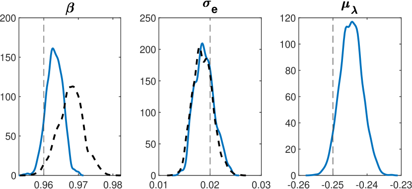
Figure 2: Posterior densities with (blue solid curves) and without (black dashed curves) conditioning on the micro data. Both sets of results use the same simulated data set. Vertical dashed lines indicate true parameter values. Posterior density estimates from the 9,000 retained MCMC draws using Matlab’s ksdensity function with default settings. The third display omits the macro-only results, since $\mu_{\lambda}$ is not identified from macro data alone.

Figure 2 shows that both macro and micro data can be useful or even essential for estimating some parameters, but not others. The figure depicts the posterior densities of the three parameters, on a single sample of simulated data. The full-information posterior (blue solid curves) is concentrated close to the true values of the three parameters (which are marked by vertical thin dashed lines). The figure also shows the posterior density without conditioning on the micro data (black dashed curves). The household discount factor $\beta$ is an important determinant of not just aggregate variables, but also the heterogeneous actions of the micro agents in the economy. Ignoring the micro data leads to substantially less accurate inference about $\beta$ in this simulation, as the macro-only posterior is less precisely centered around the true value as well as more diffuse than the full-information posterior. Nevertheless, macro data clearly does meaningfully contribute to pinning down the parameter $\beta$. More starkly, $\mu_{\lambda}$ can only be identified from the cross section, since by construction the macro aggregates are not influenced by the distribution of the individual permanent productivity draws $\lambda_{i}$. In contrast, essentially all the information about the measurement error standard deviation $\sigma_{e}$ comes from the macro data, again by construction. Thus, our results here illustrate the general lesson that both macro and micro data can be either essential, useful, or irrelevant for estimating different parameters.

Heterogeneous household model: Consumption policy function, employed

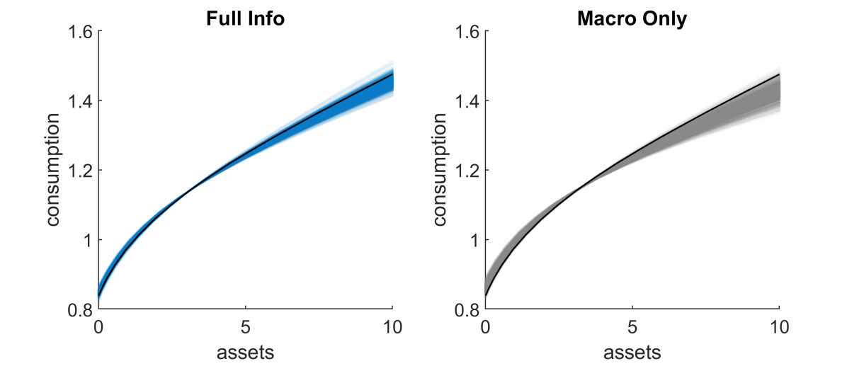
Figure 3: Estimated steady state consumption policy function for employed households, either using both micro and macro data (left panel) or only using macro data (right panel). The thick black curve is computed under the true parameters. The thin lines are 900 posterior draws (computed using every 10th MCMC draw after burn-in). X-axes are normalized asset holdings $a_{i,t}$.

Figure 3 shows that efficient use of the micro data leads to substantially more precise estimates of the steady state consumption policy function for employed households. The left panel shows that full-information posterior draws of the consumption policy function (thin curves) are fairly well centered around the true function (thick curve), as is expected given the accurate inference about $\beta$ depicted in Figure 2. In contrast, the right panel shows that macro-only posterior draws are less well centered and exhibit higher variance, especially for households with high or low current asset holdings. The added precision afforded by efficient use of the micro data translates into more precise estimates of the marginal propensity to consume (the derivative of the consumption policy function) at the extremes of the asset distribution. This is potentially useful when analyzing the two-way feedback effect between macroeconomic policies and redistribution (Auclert, 2019).

Het. household model: Impulse responses of asset distribution, employed

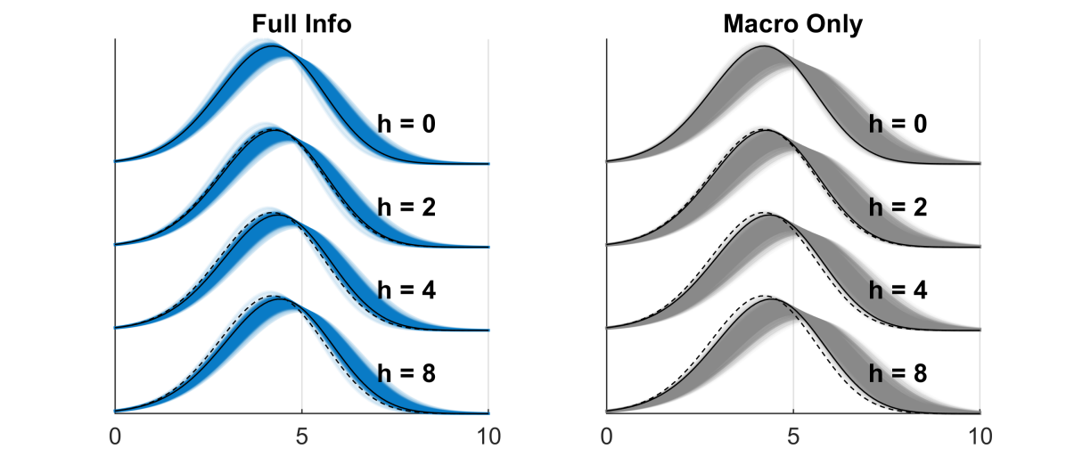
Figure 4: Estimated impulse response function of employed households’ asset distribution with respect to an aggregate productivity shock, either using both micro and macro data (left panel) or only using macro data (right panel). The thin lines are 900 posterior draws (computed using every 10th MCMC draw after burn-in). X-axes are normalized asset holdings $a_{i,t}$. The four rows in each panel are the asset densities at impulse response horizons 0 (impact), 2, 4, and 8. The black dashed and black solid curves are the steady state density and the impulse response, respectively, computed under the true parameters. On impact the true impulse response equals the steady state density, since households’ portfolio choice is predetermined.

The extra precision afforded by micro data also sharpens inference on the impulse response function of the asset distribution with respect to an aggregate productivity shock. Figure 4 shows full-information (left panel) and macro-only (right panel) posterior draws of the impulse response function of employed households’ asset holding density, in the periods following a 5% aggregate productivity shock. Once again, the full-information results have substantially lower variance. Following the shock, there is a noticeable movement of the asset distribution computed under the true parameters (black solid curve). At horizon $h=8$, the mean increases by 0.16 relative to the steady state (black dashed curve), the variance increases by 0.10, and the third central moment decreases by 0.06. However, the true movement in the asset distribution is not so large relative to the estimation uncertainty. This further motivates the use of an efficient inference method that validly takes into account all estimation uncertainty.

The previous qualitative conclusions hold up in repeated simulations from the calibrated model. We repeat the MCMC estimation exercise on 10 different simulated data sets. Figure 5 plots all 10 full-information and macro-only posterior densities for the three parameters on the same plot. Notice that the full-information densities for $\beta$ systematically concentrate closer to the true value than the macro-only posteriors do, as in Figure 2.

Heterogeneous household model: Posterior density, multiple simulations

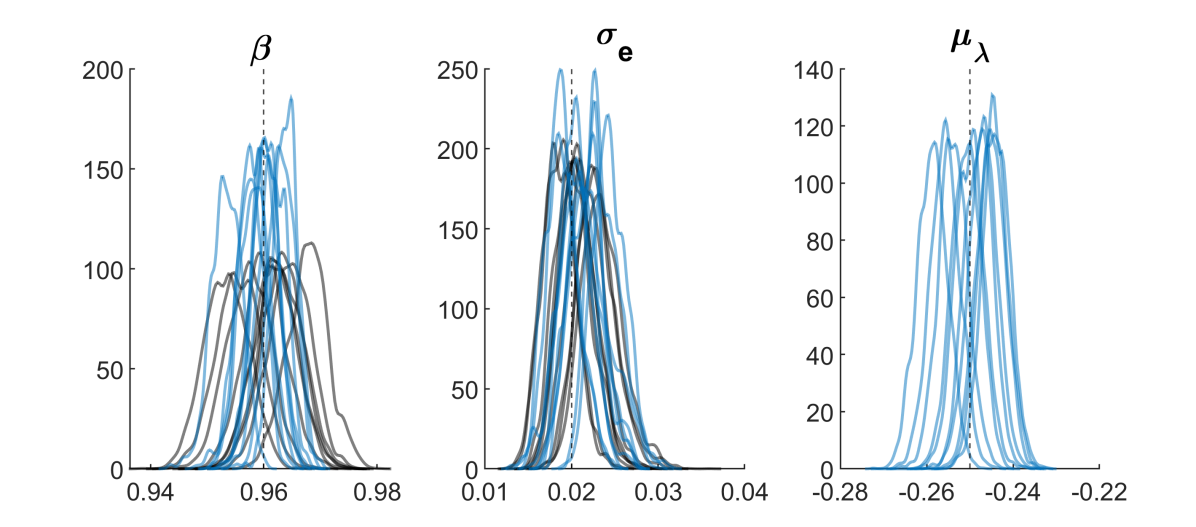
Figure 5: Posterior densities with (blue curves) and without (gray curves) conditioning on the micro data, for 10 different simulated data sets. See also caption for Figure 2.

Our inference approach is valid in the usual Bayesian sense no matter how small the sample size is. In LABEL:fig:example_hh_postdens_N100 of LABEL:sec:example_hh_results we show that the full-information approach still yields useful inference about the model parameters if we only observe $N=100$ observations every ten periods (instead of $N=1000$ as above).

4.4 Comparison with moment-based methods

In this subsection, we compare the above full-information results with a moment-based inference approach, to shed light on the theoretical comparison in Section 3.3. Due to the unobserved individual heterogeneity parameter $\lambda_{i}$, fixed-dimensional sufficient statistics do not exist in this model with the given observables. Hence, we follow empirical practice and compute an ad hoc selection of cross-sectional moments, including the sample mean, variance, and third central moment of household after-tax income. We compute the moments separately for the groups of employed and unemployed households, in each period $t=10,20,\dots,100$ where micro data is observed. We consider three moment-based approaches with different numbers of observables: The “1st Moment” approach only incorporates time series of sample means, the “2nd Moment” approach incorporates both sample means and variances, and the “3rd Moment” approach incorporates sample moments up to the third order.

Once we compute the time series of cross-sectional moments on the simulated data, we treat them as additional time series observables and proceed as in the “Macro Only” approach considered earlier. To account for the sampling uncertainty in the cross-sectional moments, we appeal to a Central Limit Theorem and treat the moments as jointly Gaussian, which is equivalent to adding measurement error in those state space equations that correspond to the moments. A natural and practical way to construct the variance-covariance matrix of the measurement error is to estimate its elements using higher-order sample moments of micro data. The variance-covariance matrix is actually time-varying according to the structural model, but since this would be challenging to account for, we treat it as fixed over the sample. LABEL:sec:moment_vcv provides the details of how we estimate the variance-covariance matrix. The computation time of the moment-based likelihood functions is not much faster than our full-information approach, since the evaluation of the micro likelihood (which is specific to the full-information method) takes approximately the same amount of time as the calculation of the model’s steady state (which is common to all methods), when implemented on a research cluster with 20 parallel workers.

We compare the shape and location of the likelihood functions for the full-information and moment-based methods. For graphical clarity, we vary a single parameter at a time, keeping the other parameters at their true values. Figure 6 plots the univariate log likelihood functions of all inference approaches based on one typical simulated data set. Since we are interested in the curvature of the likelihood functions near their maxima, and not the overall level of the functions, we normalize each curve by subtracting its maximum.

Heterogeneous household model: Likelihood comparison

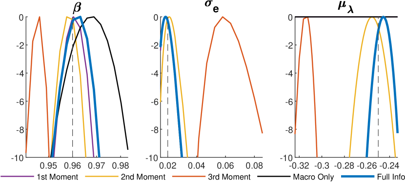
Figure 6: Comparison of log likelihoods across inference methods, based on one typical simulated data set. Each panel depicts univariate deviations of a single parameter while keeping all other parameters at their true values. The maximum of each likelihood curve is normalized to be zero. Vertical dashed lines indicate true parameter values. The “1st Moment” and “Macro Only” curves are flat on the right panel, since $\mu_{\lambda}$ is not identified from this data alone. For results across 10 different simulated data sets, see Figure 9 in Section A.4.

Figure 6 shows that the moment-based likelihoods do not approximate the efficient full-information likelihood well, with the “3rd Moment” likelihood being particularly inaccurately centered. There are two reasons for this. First, as discussed in Section 3.3, there is no theoretical sufficient statistics in this setup, so all the moment-based approaches incur some efficiency loss. Second, the sampling distributions of higher-order sample moments are not well approximated by Gaussian distributions in finite samples, and the measurement error variance-covariance matrix depends on even higher-order moments, which are poorly estimated. A separate issue is that the individual heterogeneity parameter $\mu_{\lambda}$ cannot even be identified using the “1st Moment” approach, since this parameter does not influence first moments of the micro data. The “2nd Moment” likelihood is not entirely misleading but nevertheless differs meaningfully from the full-information likelihood. Figure 9 in Section A.4 confirms that the aforementioned qualitative conclusions hold up across 10 different simulated data sets.

To summarize, even in this relatively simple model, the moment-based methods we consider lead to a poor approximation of the full-information likelihood, and the inference can be highly sensitive to the choice of which moments to include. It is possible that other implementations of the moment-based approach would work better in particular applications. Nevertheless, any moment-based approach will require challenging ad hoc choices, such as which moments to use and how to account for their sampling uncertainty. No such choices are required by the efficient full-information approach developed in this paper.

5 Illustration: Heterogeneous firm model

As our second proof-of-concept example, we estimate a version of the heterogeneous firm model of Khan and Thomas (2008). In addition to showing that our general inference approach can be applied outside the specific Krusell and Smith (1998) family of models, we use this section to illustrate how sample selection or data censoring can easily be accommodated in our method.

5.1 Model, data, and prior

A continuum of heterogeneous firms are subject to both idiosyncratic and aggregate productivity shocks. Investment is subject to non-convex adjustment costs. Specifically, firm $i$’s investment $I_{i,t}$ is free if $|I_{i,t}/k_{i,t}|\leq a$, where $k_{i,t}$ is the firm-specific capital stock, and $a\geq 0$ is a parameter. Otherwise, firms pay a fixed adjustment cost of $\xi_{i,t}$ in units of labor. $\xi_{i,t}$ is drawn at the beginning of every period from a uniform distribution on the interval $[0,\bar{\xi}]$, independently across firms and time. Here $\bar{\xi}\geq 0$ is another parameter. In addition to the aggregate productivity shock, there is a second aggregate shock that affects investment efficiency. The representative household has additively separable preferences over log consumption and (close to linear) leisure time. For brevity, we relegate the details of the model to LABEL:sec:example_firm_details, which entirely follows Winberry’s (2018) version of the Khan and Thomas (2008) model.

We aim to estimate the adjustment cost parameters $\bar{\xi}$ and $a$. Khan and Thomas (2008) showed that these parameters have little impact on the aggregate macro implications of the model in their preferred calibration; hence, micro data is needed. We keep all other parameters fixed at their true values for simplicity. LABEL:sec:example_firm_prod provides results for an alternative exercise where we instead estimate the parameters of the firms’ idiosyncratic productivity process; the key messages are qualitatively similar to those presented below.

We adopt the annual calibration of Winberry (2018), which in turn follows Khan and Thomas (2008), see LABEL:sec:example_firm_calib. However, we make an exception in setting the firm’s idiosyncratic log productivity AR(1) parameter $\rho_{\epsilon}=0.53$, following footnote 5 in Khan and Thomas (2008). We then adjust the log productivity innovation standard deviation $\sigma_{\epsilon}=0.0364$, so that the variance of the idiosyncratic log productivity process is unchanged from the baseline calibration in Khan and Thomas (2008) and Winberry (2018). The macro implications of our calibration are virtually identical to the baseline in Khan and Thomas (2008), as those authors note.

We assume that the econometrician observes time series on aggregate output and investment, as well as repeated cross sections of micro data on firms’ capital and labor inputs. We simulate macro data with sample size $T=50$, while micro cross sections of size $N=1000$ are observed at each point in time $t=1,\dots,50$. Unlike in Section 4, we do not add measurement error to the macro observables.

The prior on $(\bar{\xi},a)$ is chosen to be flat in the natural parameter space.

5.2 Computation

As in Section 4, we solve and simulate the model using the Winberry (2018) Dynare solution method. We follow Winberry (2018) and approximate the cross-sectional density of the firms’ micro state variables (log capital and idiosyncratic productivity) with a multivariate normal distribution. Computation of the micro sampling density is simple, since – conditional on macro states – the micro observables (capital and labor) are log-linear transformations of these micro state variables. We use $J=500$ smoothing draws to compute the unbiased likelihood estimate. The MCMC routine is the same as in Section 4. The starting values are selected by a rough grid search on the simulated data. We generate 10,000 draws and discard the first 1,000 as burn-in. Likelihood evaluation using 20 parallel cores is several times faster than computing the model’s steady state.

5.3 Results

Despite the finding in Khan and Thomas (2008) that macro data is essentially uninformative about the firms’ adjustment cost parameters, these are accurately estimated when the micro data is used also. Figure 7 shows the posterior densities of $\bar{\xi}$ and $a$ computed on 10 different simulated data sets. The posterior distribution of each parameter is systematically concentrated close to the true parameter values. We refrain from visually comparing these results with inference that relies only on macro data, since the macro likelihood is almost entirely flat as a function of $(\bar{\xi},a)$, consistent with Khan and Thomas (2008). Thus, micro data is essential to inference about these parameters. This finding is broadly consistent with Bachmann and Bayer (2014), who show that the dynamics of the cross-sectional dispersion of firm investment are very informative about the nature of firm-level frictions.

Heterogeneous firm model: Posterior density, multiple simulations

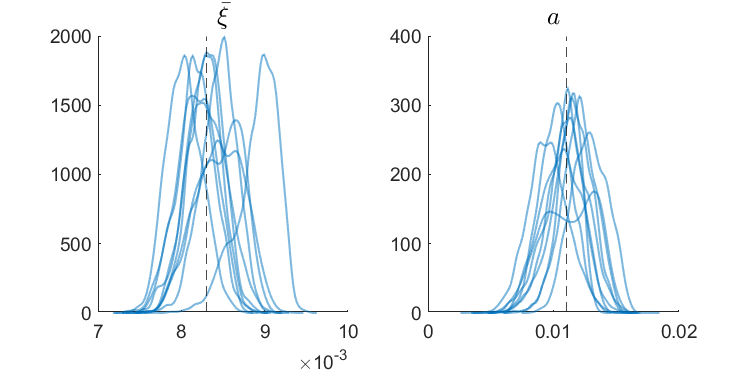
Figure 7: Posterior densities across 10 simulated data sets. Vertical dashed lines indicate true parameter values. Posterior density estimates from the 9,000 retained MCMC draws using Matlab’s ksdensity function with default settings.

5.4 Correcting for imperfect sampling of micro data

One advantage of the likelihood approach adopted in this paper is that standard techniques can be applied to correct for sample selection or censoring in the micro data. This is highly relevant for applied work, since household or firm surveys are often subject to known data imperfections, even beyond measurement error.

Valid inference about structural parameters merely requires that the micro sampling density $p(y_{i,t}\mid z_{t},\theta)$ introduced in Section 2.1 accurately reflects the sampling mechanism, including the effects of selection or censoring. Hence, if it is known, say, that an observed variable such as household income is top-coded (i.e., censored) at the threshold $\bar{y}$, then the functional form of the density $p(y_{i,t}\mid z_{t},\theta)$ should take into account that the observed data equals a transformation $y_{i,t}=\min\{\tilde{y}_{i,t},\bar{y}\}$ of the theoretical household income $\tilde{y}_{i,t}$ in the DSGE model. The likelihood functions of such limited dependent variable sampling models are well known and readily looked up, see for example Wooldridge (2010, chapters 17 and 19). We provide one illustration below.

Other approaches to estimating heterogeneous agent models do not handle data imperfections as easily or efficiently. For example, inference based on cross-sectional moments of micro observables may require lengthy derivations to adjust the moment formulas for selection or censoring, especially for higher moments. Moreover, even in models where low-dimensional sufficient statistics exist for the underlying micro variables, cf. Section 3.3, the imperfectly observed micro data may not afford such sufficient statistics. In contrast, our likelihood-based approach is automatically efficient, and the adjustments needed to account for common types of data imperfections can be looked up in microeconometrics textbooks.

Illustration: Selection on outcomes.

We illustrate the previous points by adding an endogenous selection mechanism to the sampled micro data in the heterogeneous firm model. Assume that instead of observing a representative sample of firms every period, we observe the draws for those firms whose employment in that period exceeds the 90th percentile of the steady-state cross-sectional distribution of employment. To make the effective micro sample size comparable to that in Section 5.3, we here set the per-period micro sample size before selection equal to $N=10000$. That is, out of 10000 potential draws in a period, we only observe the capital and labor inputs of the approximately 1000 largest firms. Though stylized, this sampling mechanism is intended to mimic the real-world phenomenon that databases such as Compustat tend to only cover the largest active firms in the economy.

To adjust the likelihood for selection, we combine the model-implied cross-sectional distribution of the idiosyncratic state variables with the functional form of the selection mechanism. Let $g_{t}(\epsilon,k)$ be the cross-sectional distribution of idiosyncratic log productivity $\epsilon_{i,t}$ and log capital $k_{i,t}$ at time $t$, implied by the model (this density is approximated using an exponential family of densities, as in Winberry, 2018). In the model, log employment is given by $n_{i,t}=(\log\nu+\zeta_{t}-\log(w_{t})+\epsilon_{i,t}+\alpha k_{i,t})/(1-\nu)$, where $w_{t}$ is the aggregate wage, $\zeta_{t}$ is log aggregate TFP, and $\nu$ and $\alpha$ are the output elasticities of labor and capital in the firm production function ($\nu+\alpha<1$). Since observations $y_{i,t}=(n_{i,t},k_{i,t})^{\prime}$ are observed if and only if $n_{i,t}\geq\bar{n}$, the micro sampling density is given by the truncation formula

$$p(n_{i,t},k_{i,t}\mid z_{t},\theta)=\frac{(1-\nu)g_{t}\big{(}(1-\nu)n_{i,t}-\alpha k_{i,t}-\log\nu-\zeta_{t}+\log(w_{t}),k_{i,t}\big{)}}{\int_{-\infty}^{\infty}\int_{-\infty}^{\infty}\mathbbm{1}\big{(}\log\nu+\zeta_{t}-\log(w_{t})+\epsilon+\alpha k\geq(1-\nu)\bar{n}\big{)}g_{t}(\epsilon,k)\,d\epsilon\,dk}.$$

The selection threshold $\bar{n}$ is given by the true 90th percentile of the steady-state distribution of log employment. We assume this threshold is known to the econometrician for simplicity.

Heterogeneous firm model: Posterior densities with selection

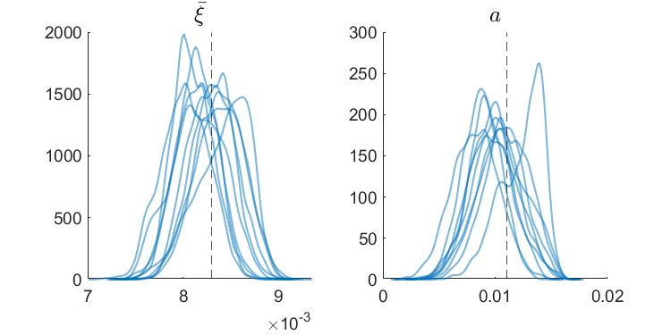
Figure 8: Posterior densities across 10 simulated data sets subject to selection. Vertical dashed lines indicate true parameter values. Posterior density estimates from the 9,000 retained MCMC draws using Matlab’s ksdensity function with default settings.

Figure 8 shows the posterior distribution of the adjustment cost parameters $(\bar{\xi},a)$ in the model with selection, across 10 simulated data sets. All settings are the same as in Section 5.3, except for (i) the selection mechanism in the simulated micro data and the requisite adjustment to the functional form of the micro likelihood function, and (ii) the pre-selection micro sample size $N=10000$ (as discussed above). The posterior distributions of the parameters of interest remain centered close to the true parameter values, with no appreciable increase in posterior uncertainty relative to Figure 7. This example demonstrates that data imperfections can be handled in a valid and efficient manner using standard likelihood techniques.

6 Extension to panel data

While our baseline procedure in Section 3 assumes the micro data to be given by repeated cross sections, we now consider settings where the micro data has a panel dimension – that is, the same cross-sectional units are observed over two or more consecutive time periods. For tractability, we focus on panel data sets where the time dimension per unit is short (similar to Papp and Reiter, 2020). One example is rotating panel survey data, where each unit is observed for a few consecutive time periods, after which it is replaced by a new, representatively sampled unit (as in the Bureau of Labor Statistics’ Consumer Expenditure Survey). Panel data sets with a large time dimension, such as detailed administrative data sets, are computationally challenging and beyond the scope of this paper.

6.1 Challenges and solutions

The main challenge in handling panel data is the need to integrate out any unobserved individual-specific state variables (such as idiosyncratic productivity or asset holdings) that influence agents’ dynamic decision rules. If the structural model directly implies a simple functional form for the one-step-ahead predictive density $p(y_{i,t}\mid y_{i,t-1},y_{i,t-2},\dots,\mathbf{z},\theta)$ of the observed data $y_{i,t}$ for individual $i$, then evaluating the micro likelihood is trivial (as in reduced-form dynamic panel data models). Unfortunately, in most settings this predictive density is not available in closed form, and must instead be computed as the integral $\int p(y_{i,t}\mid s_{i,t},\mathbf{z},\theta)p(s_{i,t}\mid y_{i,t-1},y_{i,t-2},\dots,\mathbf{z},\theta)\,ds_{i,t}$ over the latent micro state variables $s_{i,t}$. Whereas the first density in the integrand may often be available in closed form, the second density will typically not be (outside simple linear models). Hence, evaluating the integral for each $i$ and $t$ appears to be computationally infeasible in many applications, especially if the number of time periods is moderately large. Nevertheless, as we now show, it is often possible to evaluate the micro likelihood when the time dimension per unit is small, by avoiding direct evaluation of the intractable predictive density.

Our proposal for exploiting panel data utilizes the model-implied relationship between (i) the latent micro state variables $s_{i,t_{i}}$ in the initial period $t_{i}$ for individual $i$ and (ii) the micro observables $\{y_{i,t}\}_{t}$ in all observed time periods for that individual. This relation necessarily involves iterating on the dynamic micro decision rules of the agents in the economy. In the next subsection, we explain this approach by example, using the heterogeneous household model from Section 2.2. Since the main focus of this paper is repeated cross-sectional micro data, we leave a numerical exploration of the benefits of panel data for future work.

6.2 Example: Heterogeneous household model

Unlike in Section 2.2, we here assume that we observe two consecutive periods of $y_{i,t}=(\epsilon_{i,t},\iota_{i,t})$ for each household $i$, i.e., household employment and income. To implement the likelihood estimate in Section 3, we must evaluate the conditional micro density

$$p(y_{i,t},y_{i,t-1}\mid\mathbf{z},\theta)=\underbrace{p(\epsilon_{i,t},\epsilon_{i,t-1}\mid\mathbf{z},\theta)}_{=p(\epsilon_{i,t-1},\theta)p(\epsilon_{i,t}\mid\epsilon_{i,t-1},\theta)}p(\iota_{i,t},\iota_{i,t-1}\mid\epsilon_{i,t},\epsilon_{i,t-1},\mathbf{z},\theta).$$

Employment $\epsilon_{i,t}$ evolves as a simple exogenous two-state Markov process, so the challenge is to evaluate the last density on the right-hand side above.

Note that, by definition of household income,

$$\iota_{i,t-1}=\lambda_{i}\big{(}w_{t-1}[(1-\tau)\epsilon_{i,t-1}+b(1-\epsilon_{i,t-1})]+(1+r_{t-1})a_{i,t-2}\big{)},$$

and

$$\iota_{i,t}=\lambda_{i}\big{(}w_{t}[(1-\tau)\epsilon_{i,t}+b(1-\epsilon_{i,t})]+(1+r_{t})a_{t-1}^{\prime}(a_{i,t-2},\epsilon_{i,t-1})\big{)},$$

where $a_{t-1}^{\prime}(a,\epsilon)$ is the model-implied micro policy function at period $t-1$ for next-period normalized assets given current normalized assets $a$ and current employment $\epsilon$, and given the aggregate state $z_{t-1}$.

Conditional on $(\epsilon_{i,t},\epsilon_{i,t-1})$ and the macro states $\mathbf{z}$ in all periods, the observation $(\iota_{i,t},\iota_{i,t-1})$ is therefore a known transformation of the initial micro state vector $s_{i,t-1}=(\lambda_{i},a_{i,t-2})$. We can then derive $p(\iota_{i,t},\iota_{i,t-1}\mid\epsilon_{i,t},\epsilon_{i,t-1},\mathbf{z},\theta)$ by applying the change-of-variables formula to the density $p(\lambda_{i},a_{i,t-2}\mid\epsilon_{i,t},\epsilon_{i,t-1},\mathbf{z},\theta)=f(\lambda_{i}\mid\mu_{\lambda})g_{\epsilon_{i,t-1}}(a_{i,t-2}\mid\psi_{t-1})$, where $\psi_{t-1}$ denotes the parameters governing the cross-sectional distribution and is part of the aggregate state $z_{t-1}$, and the density $g_{\epsilon_{i,t-1}}(a_{i,t-2}\mid\psi_{t-1})$ is directly available from the output of the model solution procedure, as discussed in Section 2.2. Computing the Jacobian term in the change-of-variables formula requires us to evaluate the derivative $\partial a_{t-1}^{\prime}(a,\epsilon)/\partial a$, for example by applying finite differences to the function $a_{t-1}^{\prime}(a,\epsilon)$ that is outputted by the numerical model solution method.

6.3 Summary and discussion

In general terms, our proposal is to express the consecutive micro observations in terms of the latent micro state variables $s_{i,t_{i}}$ in the initial observed period $t_{i}$ for individual $i$. We can then “invert” this relation and evaluate the micro likelihood using the model-implied cross-sectional density of $s_{i,t_{i}}$ (which we also exploited previously in the repeated cross section setup). This strategy is highly context-specific as it exploits the structure of the observables and iterates on the model-implied dynamic decision rules of the agents. Though we have only illustrated the strategy for the case of two-period panel data, the idea could in principle be applied to longer panels by further iterating on the decision rules; however, this could become cumbersome when the time dimension is moderately large. As a side note, it is straightforward to allow for measurement error in the micro observables by simply adding independent noise to the density of the noise-less observables using the convolution formula.

In some models the dynamic relationship between micro states and micro observables may be sufficiently convoluted to render the above approach impractical. For such cases, we propose an alternative approach in LABEL:sec:panel_general based on artificially adding lagged state variables to the micro state vector in the numerical model solution procedure. Though this alternative approach is conceptually simple to implement, the increase in the dimension of the effective micro state vector may require more time to be spent on computing an accurate numerical solution of the model. We therefore recommend that researchers first attempt the baseline approach illustrated in the previous subsection, which does not require any modification of the numerical model solution method.

7 Conclusion

The literature on heterogeneous agent models has hitherto relied on estimation approaches that exploit ad hoc choices of micro moments and macro time series for estimation. This contrasts with the well-developed framework for full-information likelihood inference in representative agent models (Herbst and Schorfheide, 2016). We develop a method to exploit the full information content in macro and micro data when estimating heterogeneous agent models. As we demonstrate through economic examples, the joint information content available in micro and macro data is often much larger than in either of the two separate data sets. Our inference procedure can loosely be interpreted as a two-step method: First we estimate the underlying macro states from macro data, and then we evaluate the likelihood by plugging into the cross-sectional sampling densities given the estimated states. However, our method delivers finite-sample valid and fully efficient Bayesian inference that takes into account all sources of uncertainty about parameters and states. The computation time of our procedure scales well with the size of the data set, as the method lends itself to parallel computing. Unlike estimation approaches based on tracking a small number of cross-sectional moments over time, our full-information method is automatically efficient and can easily accommodate unobserved individual heterogeneity, micro measurement error, as well as data imperfections such as censoring or selection.

For clarity, we have limited ourselves to numerical illustrations with small-scale models in this paper, leaving full-scale empirical applications to future work. Our approach is computationally most attractive when the model is solved using some version of the Reiter (2009) linearization approach, since this yields simple formulas for evaluating the macro likelihood and drawing from the smoothing distribution of the latent macro states, cf. Section 3. To estimate large-scale quantitative models it would be necessary to apply now-standard dimension reduction techniques or other computational shortcuts to the linearized representation of the macro dynamics (Ahn, Kaplan, Moll, Winberry, and Wolf, 2017; Auclert, Bardóczy, Rognlie, and Straub, 2021), and we leave this to future research. Nevertheless, we emphasize that our method is in principle generally applicable, as long as there exists some way to evaluate the macro likelihood, draw from the smoothing distribution of the macro states, and evaluate the micro sampling density given the macro states.

Our research suggests several additional avenues for future research. First, it would be useful to go beyond our extension to short panel data sets in Section 6 and develop methods that are computationally feasible when the time dimension of the panel is large. Second, since our method works for a wide range of generic MCMC posterior sampling procedures, it would be interesting to investigate the scope for improving on the simple Random Walk Metropolis-Hastings algorithm that we use for conceptual clarity in our examples. Third, the goal of this paper has been to fully exploit all aspects of the assumed heterogeneous agent model when doing statistical inference; we therefore ignore the consequences of misspecification. Since model misspecification potentially affects the entire macro equilibrium and thus cannot be addressed using off-the-shelf tools from the microeconometrics literature, we leave the development of robust inference approaches to future work.

Appendix A Appendix

A.1 Proofs

A.1.1 Proof of 1

Let $\hat{m}_{t}\equiv(\hat{m}_{1,t},\dots,\hat{m}_{Q,t})^{\prime}$ denote the set of sufficient statistics in period $t$. According to the Fisher-Neyman factorization theorem, there exists a function $h(\cdot)$ such that the likelihood of the micro data in period $t$, conditional on $z_{t}$, can be factorized as

$$\prod_{i=1}^{N_{t}}p(y_{i,t}\mid z_{t},\theta) =h(y_{t})p(\hat{m}_{t}\mid N_{t},z_{t},\theta).$$ (10)

Let $\mathbf{h}(\mathbf{y})=\prod_{t\in\mathcal{T}}h(y_{t})$, $\mathbf{N}=\{N_{t}\}_{t\in\mathcal{T}}$, and $\mathbf{\hat{m}}=\{\hat{m}_{t}\}_{t\in\mathcal{T}}$, where $\mathcal{T}$ is the subset of time points with observed micro data. Then the micro likelihood, conditional on the observed macro data, can be decomposed as

$$p(\mathbf{y}\mid\mathbf{x},\theta) =\int p(\mathbf{y}\mid\mathbf{z},\theta)p(\mathbf{z}\mid\mathbf{x},\theta)\,d\mathbf{z}$$

$$=\mathbf{h}(\mathbf{y})\int p(\mathbf{\hat{m}}\mid\mathbf{N},\mathbf{z},\theta)p(\mathbf{z}\mid\mathbf{x},\theta)\,d\mathbf{z}$$ (11)

$$=\mathbf{h}(\mathbf{y})p(\mathbf{\hat{m}}\mid\mathbf{N},\mathbf{x},\theta).$$ (12)

The expression (12) implies that $\mathbf{\hat{m}}$ is a set of sufficient statistics for $\theta$, based again on the Fisher-Neyman factorization theorem. ∎

A.1.2 Proof of 1

Let $m_{t}$ be a vector of population counterparts of the cross-sectional sufficient statistics of the micro states $s_{i,t}$. We may view $m_{t}$ as part of the macro state vector $z_{t}$. According to the exponential polynomial setup,

$$p(s_{i,t}\mid z_{t},\theta) =p(s_{i,t}\mid m_{t})$$

$$=\exp\left[\tilde{\varphi}_{0}(m_{t})+\sum_{\ell=1}^{Q}\tilde{\varphi}_{\ell}(m_{t})\tilde{\mathfrak{m}}_{\ell}(s_{i,t})\right].$$

$\tilde{\mathfrak{m}}_{\ell}(s_{i,t})$ takes the form $s_{i,t,1}^{p_{1}}s_{i,t,2}^{p_{2}}\cdots s_{i,t,d_{s}}^{p_{d_{s}}}$ with $p_{k}$ being positive integers and $1\leq\sum_{k=1}^{d_{s}}p_{k}\leq q$, where $q$ is the order of the exponential polynomial. The potential number of sufficient statistics $Q$ equals $\binom{q+d_{s}}{q}-1$, i.e., the number of complete homogeneous symmetric polynomials.

Making the change of variables in (9), we have

$$p(y_{i,t}\mid z_{t},\theta) =\exp\left[\tilde{\varphi}_{0}(m_{t})+\sum_{\ell=1}^{Q}\tilde{\varphi}_{\ell}(m_{t})\tilde{\mathfrak{m}}_{\ell}\big{(}B_{1}(z_{t},\theta)\Upsilon(y_{i,t})+B_{0}(z_{t},\theta)\big{)}\right]$$

$$\qquad\times\left|\det\left(B_{1}(z_{t},\theta)\frac{\partial\Upsilon(y_{i,t})}{\partial y_{i,t}}\right)\right|$$

$$\equiv\exp\left[\varphi_{0}(z_{t},\theta)+{\mathfrak{m}}_{0}(y_{i,t})+\sum_{\ell=1}^{Q}\varphi_{\ell}(z_{t},\theta){\mathfrak{m}}_{\ell}(y_{i,t})\right].$$

Given assumptions 2.a and 2.b, the potential number of sufficient statistics $Q$ remains the same. Now the sufficient statistics can be expressed as ${\mathfrak{m}}_{\ell}(y_{i,t})\equiv\tilde{\mathfrak{m}}_{\ell}(\Upsilon(y_{i,t}))$ and the corresponding $\varphi_{\ell}(z_{t},\theta)$ can be obtained by rearranging terms and collecting coefficients on ${\mathfrak{m}}_{\ell}(y_{i,t})$. For the determinant of the Jacobian, condition 2 implies that both $B_{1}(z_{t},\theta)$ and $\frac{\partial\Upsilon(y_{i,t})}{\partial y_{i,t}}$ are non-singular square matrices, so $\det\left(B_{1}(z_{t},\theta)\frac{\partial\Upsilon(y_{i,t})}{\partial y_{i,t}}\right)=\det\left(B_{1}(z_{t},\theta)\right)\det\left(\frac{\partial\Upsilon(y_{i,t})}{\partial y_{i,t}}\right)$. Hence, both $\log\left|\det\left(B_{1}(z_{t},\theta)\right)\right|$ and $\log\left|\det\left(\frac{\partial\Upsilon(y_{i,t})}{\partial y_{i,t}}\right)\right|$ are finite and can be absorbed into $\varphi_{0}(z_{t},\theta)$ and ${\mathfrak{m}}_{0}(y_{i,t})$, respectively.

Thus, the micro likelihood fits into the general form in 1, and the sufficient statistics are given by

$$\hat{m}_{\ell,t}=\frac{1}{N_{t}}\sum_{i=1}^{N_{t}}{\mathfrak{m}}_{\ell}(y_{i,t})=\frac{1}{N_{t}}\sum_{i=1}^{N_{t}}\tilde{\mathfrak{m}}_{\ell}(\Upsilon(y_{i,t})),\quad\ell=1,\dots,Q.\qed$$

A.2 Non-existence of sufficient statistics: Details

Can we generalize beyond the sufficient conditions in 1? The key is that in (7), the terms inside the exponential should be additive and each term should take the form $\varphi_{\ell}(z_{t},\theta){\mathfrak{m}}_{\ell}(y_{i,t})$, which ensures that the cross-sectional moments can be calculated using micro data as in equation (8) and the multiplicative term $\mathbf{h}(\mathbf{y})$ can be taken out of the integral in equation (11). Building on the analysis of Section 3.3, here are more details regarding cases where there are no sufficient statistics in general.

1. $s_{i,t}=B_{1}(z_{t},\theta)\Upsilon(y_{i,t},z_{t})+B_{0}(z_{t},\theta)$, i.e., $y_{i,t}$ and $z_{t}$ are neither additively nor multiplicatively separable.

2. The model features unobserved individual heterogeneity and/or micro measurement error. Since these two cases are observationally equivalent in a repeated cross section framework, we focus on the the former. Letting $\lambda_{i}$ denote the unobserved individual heterogeneity, we can extend (9) to $s_{i,t}=\tilde{\Upsilon}(y_{i,t},\lambda_{i},z_{t},\theta)\equiv B_{1}(\lambda_{i},z_{t},\theta)\Upsilon(y_{i,t},\lambda_{i})+B_{0}(\lambda_{i},z_{t},\theta)$, which is the most general setup allowing $\lambda_{i}$ to affect all terms in the expression. If $\lambda_{i}$ is independent of $s_{i,t}$ conditional on $(z_{t},\theta)$, we have $p(s_{i,t},\lambda_{i}\mid z_{t},\theta)=p(s_{i,t}\mid m_{t})p(\lambda_{i}\mid\theta)$ (recall the notation in the proof of 1). Accordingly,

   $$p(y_{i,t}\mid z_{t},\theta)=\int p(\tilde{\Upsilon}(y_{i,t},\lambda_{i},z_{t},\theta)\mid m_{t})\left|\det\left(B_{1}(\lambda_{i},z_{t},\theta)\frac{\partial\Upsilon(y_{i,t},\lambda_{i})}{\partial y_{i,t}}\right)\right|p(\lambda_{i}\mid\theta)\,d\lambda_{i}.$$

   If $\lambda_{i}$ appears in $B_{1}$, $B_{0}$, or $\Upsilon$, then $p(y_{i,t}\mid z_{t},\theta)$ may not belong to the exponential family after integrating out $\lambda_{i}$. That said, we can construct special cases where sufficient statistics do exist. For example, if $s_{i,t}=B_{1}(z_{t},\theta)\Upsilon(y_{i,t})+B_{0}(z_{t},\theta)+B_{2}(z_{t},\theta)\lambda_{i}$ and both $p(s_{i,t}\mid m_{t})$ and $p(\lambda_{i}\mid\theta)$ follow Gaussian distributions.

3. $d_{s}>d_{y}$: For example, suppose $s_{i,t}$ is two-dimensional whereas $y_{i,t}$ is one-dimensional, say $y_{i,t}=s_{1,i,t}$, $y_{i,t}=s_{1,i,t}+s_{2,i,t}$, or $y_{i,t}=s_{1,i,t}s_{2,i,t}$. We can first expand the $y_{i,t}$ in (9) to $\tilde{y}_{i,t}=(y_{i,t},s_{2,i,t})^{\prime}$ and then integrate out $s_{2,i,t}$. However, after the integration, the resulting micro likelihood as a function of $y_{i,t}$ may not take the exponential family form anymore.

A.3 Sampling distribution of cross-sectional moments: Example

As alluded to in Section 3.3, here is a simple example demonstrating that $p(\hat{m}_{t}\mid N_{t},z_{t},\theta)$ is not linear Gaussian in finite samples, and therefore neither is $p(\mathbf{\hat{m}}\mid\mathbf{N},\mathbf{x},\theta)$. Suppose $y_{i,t}=s_{i,t}$ is a scalar and $p(s_{i,t}\mid m_{t})$ is Gaussian, i.e., a second-order exponential polynomial. Let $\hat{m}_{1,t}=\frac{1}{N_{t}}\sum_{i=1}^{N_{t}}s_{i,t}$ and $\hat{m}_{2,t}=\frac{1}{N_{t}}\sum_{i=1}^{N_{t}}(s_{i,t}-\hat{m}_{1,t})^{2}$ with $m_{1,t}$ and $m_{2,t}$ being their population counterparts. Then standard calculations yield

$$p(\hat{m}_{t}\mid N_{t},z_{t},\theta)=p(\hat{m}_{t}\mid m_{t})=\phi\left(\hat{m}_{1,t};\,m_{1,t},\frac{m_{2,t}}{N_{t}}\right)p_{\chi^{2}}\left(\frac{N_{t}\hat{m}_{2,t}}{m_{2,t}};\,N_{t}-1\right),$$

where $\phi(x;\mu,\sigma^{2})$ represents the probability distribution function (pdf) of a Gaussian distribution with mean $\mu$ and variance $\sigma^{2}$, and $p_{\chi^{2}}(x;\nu)$ is the pdf of a chi-squared distribution with $\nu$ degrees of freedom. We can see that the latter is not linear Gaussian. Moreover, when $p(s_{i,t}\mid m_{t})$ follows a higher order exponential polynomial, the characterization of $p(\hat{m}_{t}\mid N_{t},z_{t},\theta)$ would be even more complicated without a closed-form expression.

A.4 Heterogeneous household model: Likelihood comparison

Complementing the results for a single simulated data set in Section 4.4, Figure 9 compares log likelihoods for the different inference methods across 10 different simulated data sets. Here different inference methods are exhibited in different rows. Similar to Figure 6, each column depicts univariate deviations of a single parameter while keeping all other parameters at their true values. There are 10 likelihood curves in each panel, corresponding to the 10 simulated data sets. The maximum of each likelihood curve is normalized to be zero. Vertical dashed lines indicate true parameter values. The “1st Moment” and “Macro Only” curves are flat on the right panels of the second and the last rows, since $\mu_{\lambda}$ is not identified from this data alone. We conclude from the figure that the full-information likelihood is systematically well-centered and tightly concentrated around the true parameter values, whereas the various moment-based likelihoods are poorly centered, exhibit less curvature, and/or shift around substantially across simulations.

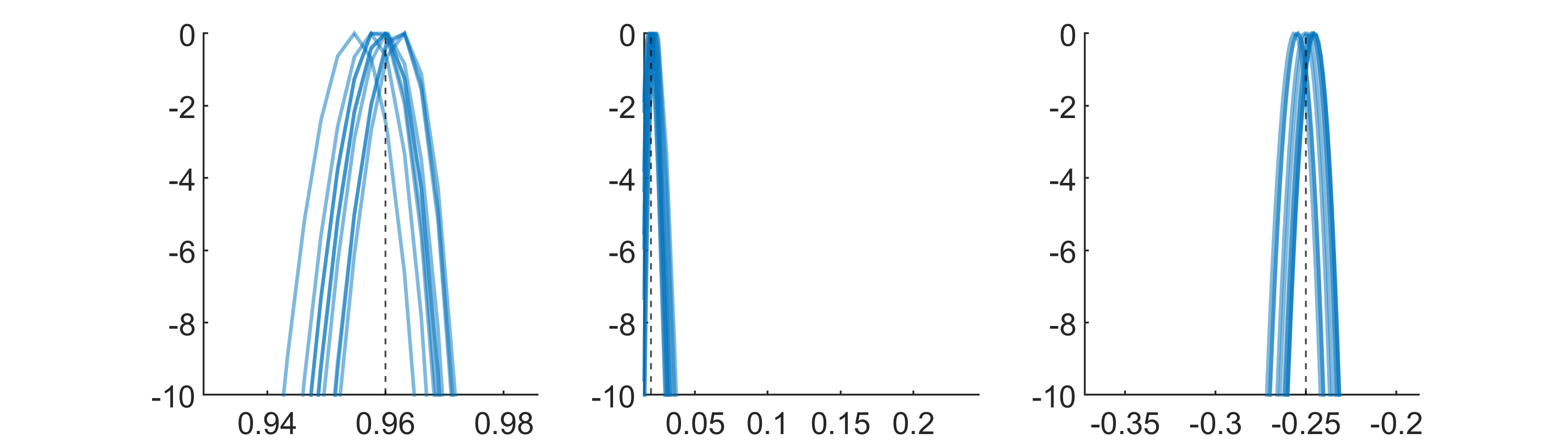
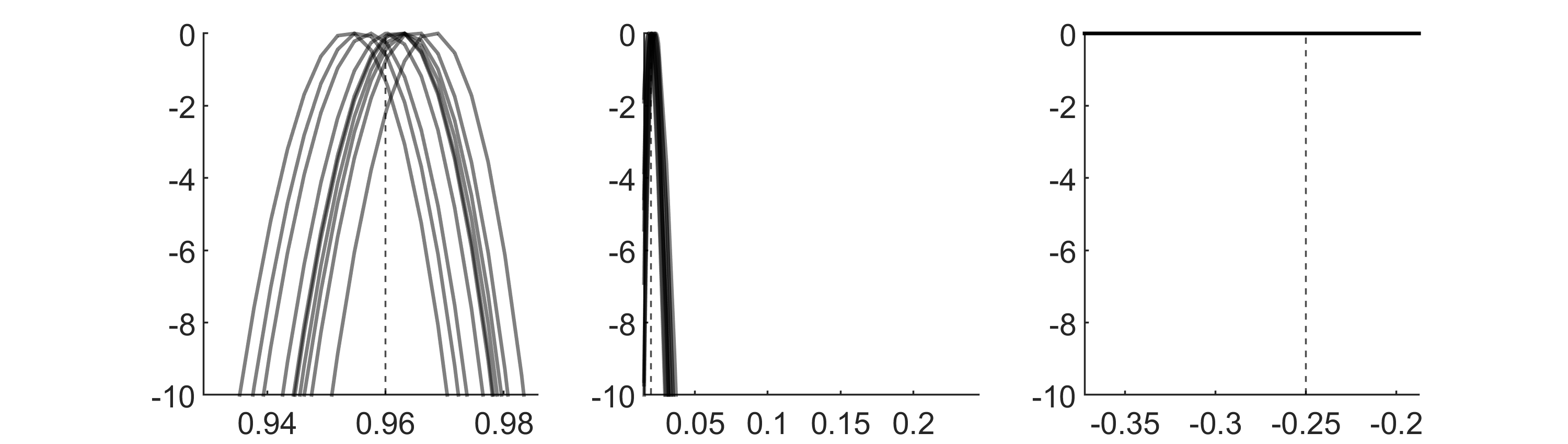
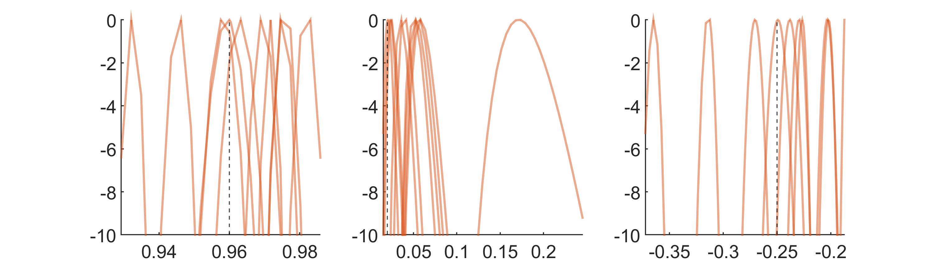
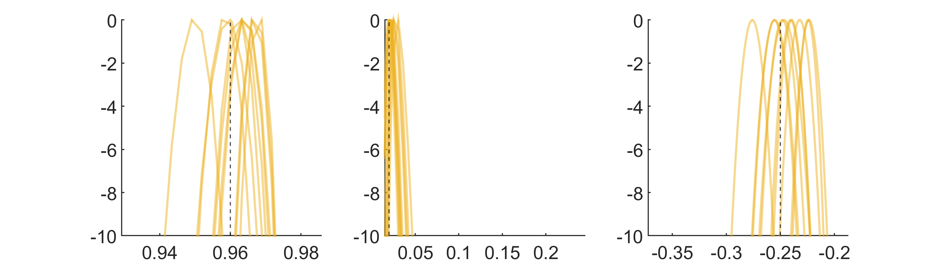
Het. household model: Likelihood comparison, multiple simulations
    $\beta$                              $\sigma_{e}$                              $\mu_{\lambda}$ Full Info Macro Only 3rd Moment 2nd Moment 1st Moment

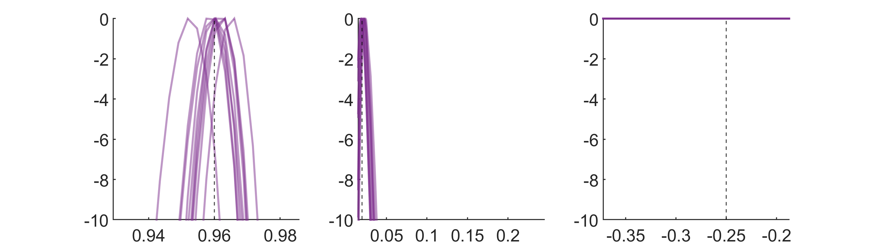
Figure 9: Comparison of log likelihood functions across 10 different simulated data sets. See the description in Section A.4.

References

- (1)
- Acharya, Negro, and Dogra (2020) Acharya, S., M. D. Negro, and K. Dogra (2020): “Estimating HANK: Macro Time Series and Micro Moments,” Paper presented at the 2021 North American Winter Meeting of the Econometric Society.
- Adjemian, Bastani, Juillard, Karamé, Maih, Mihoubi, Perendia, Pfeifer, Ratto, and Villemot (2011) Adjemian, S., H. Bastani, M. Juillard, F. Karamé, J. Maih, F. Mihoubi, G. Perendia, J. Pfeifer, M. Ratto, and S. Villemot (2011): “Dynare: Reference Manual Version 4,” Dynare Working Papers 1, CEPREMAP.
- Ahn, Kaplan, Moll, Winberry, and Wolf (2017) Ahn, S., G. Kaplan, B. Moll, T. Winberry, and C. Wolf (2017): “When Inequality Matters for Macro and Macro Matters for Inequality,” in NBER Macroeconomics Annual, Volume 32, ed. by J. A. Parker, and M. Woodford, pp. 1–75. University of Chicago Press.
- Andrieu, Doucet, and Holenstein (2010) Andrieu, C., A. Doucet, and R. Holenstein (2010): “Particle Markov chain Monte Carlo methods,” Journal of the Royal Statistical Society: Series B, 72(3), 269–342.
- Arellano and Bonhomme (2017) Arellano, M., and S. Bonhomme (2017): “Nonlinear Panel Data Methods for Dynamic Heterogeneous Agent Models,” Annual Review of Economics, 9(1), 471–496.
- Atchadé and Rosenthal (2005) Atchadé, Y. F., and J. S. Rosenthal (2005): “On adaptive Markov chain Monte Carlo algorithms,” Bernoulli, 11(5), 815–828.
- Auclert (2019) Auclert, A. (2019): “Monetary Policy and the Redistribution Channel,” American Economic Review, 109(6), 2333–2367.
- Auclert, Bardóczy, Rognlie, and Straub (2021) Auclert, A., B. Bardóczy, M. Rognlie, and L. Straub (2021): “Using the Sequence-Space Jacobian to Solve and Estimate Heterogeneous-Agent Models,” Econometrica, 89(5), 2375–2408.
- Auclert, Rognlie, and Straub (2020) Auclert, A., M. Rognlie, and L. Straub (2020): “Micro Jumps, Macro Humps: Monetary Policy and Business Cycles in an Estimated HANK Model,” NBER Working Paper 26647.
- Bachmann and Bayer (2014) Bachmann, R., and C. Bayer (2014): “Investment Dispersion and the Business Cycle,” American Economic Review, 104(4), 1392–1416.
- Bayer, Born, and Luetticke (2020) Bayer, C., B. Born, and R. Luetticke (2020): “Shocks, Frictions, and Inequality in US Business Cycles,” CEPR Discussion Paper 14364.
- Challe, Matheron, Ragot, and Rubio-Ramirez (2017) Challe, E., J. Matheron, X. Ragot, and J. F. Rubio-Ramirez (2017): “Precautionary saving and aggregate demand,” Quantitative Economics, 8(2), 435–478.
- Chang, Chen, and Schorfheide (2021) Chang, M., X. Chen, and F. Schorfheide (2021): “Heterogeneity and Aggregate Fluctuations,” NBER Working Paper 28853.
- Chang, Gomes, and Schorfheide (2002) Chang, Y., J. F. Gomes, and F. Schorfheide (2002): “Learning-by-Doing as a Propagation Mechanism,” American Economic Review, 92(5), 1498–1520.
- Durbin and Koopman (2002) Durbin, J., and S. J. Koopman (2002): “A simple and efficient simulation smoother for state space time series analysis,” Biometrika, 89(3), 603–616.
- Fernández-Villaverde, Hurtado, and Nuño (2019) Fernández-Villaverde, J., S. Hurtado, and G. Nuño (2019): “Financial Frictions and the Wealth Distribution,” NBER Working Paper 26302.
- Flury and Shephard (2011) Flury, T., and N. Shephard (2011): “Bayesian Inference Based Only on Simulated Likelihood: Particle Filter Analysis of Dynamic Economic Models,” Econometric Theory, 27(05), 933–956.
- Hahn, Kuersteiner, and Mazzocco (2022) Hahn, J., G. Kuersteiner, and M. Mazzocco (2022): “Central Limit Theory for Combined Cross-Section and Time Series,” Manuscript, arXiv:1610.01697.
- Hasumi and Iiboshi (2019) Hasumi, R., and H. Iiboshi (2019): “A Bayesian Estimation of HANK models with Continuous Time Approach: Comparison between US and Japan,” Munich Personal RePEc Archive Paper No. 92292.
- Herbst and Schorfheide (2016) Herbst, E., and F. Schorfheide (2016): Bayesian Estimation of DSGE Models, Econometric and Tinbergen Institutes Lectures. Princeton University Press.
- Imbens and Lancaster (1994) Imbens, G. W., and T. Lancaster (1994): “Combining Micro and Macro Data in Microeconometric Models,” Review of Economic Studies, 61(4), 655–680.
- Kaplan and Violante (2018) Kaplan, G., and G. L. Violante (2018): “Microeconomic Heterogeneity and Macroeconomic Shocks,” Journal of Economic Perspectives, 32(3), 167–194.
- Khan and Thomas (2008) Khan, A., and J. K. Thomas (2008): “Idiosyncratic Shocks and the Role of Nonconvexities in Plant and Aggregate Investment Dynamics,” Econometrica, 76(2), 395–436.
- Krueger, Mitman, and Perri (2016) Krueger, D., K. Mitman, and F. Perri (2016): “Macroeconomics and Household Heterogeneity,” in Handbook of Macroeconomics, Volume 2, ed. by J. B. Taylor, and H. Uhlig, chap. 11, pp. 843–921. Elsevier.
- Krueger, Perri, Pistaferri, and Violante (2010) Krueger, D., F. Perri, L. Pistaferri, and G. L. Violante (2010): “Cross-sectional facts for macroeconomists,” Review of Economic Dynamics, 13(1), 1–14.
- Krusell and Smith (1998) Krusell, P., and A. A. Smith (1998): “Income and Wealth Heterogeneity in the Macroeconomy,” Journal of Political Economy, 106(5), 867–896.
- Mongey and Williams (2017) Mongey, S., and J. Williams (2017): “Firm dispersion and business cycles: Estimating aggregate shocks using panel data,” Manuscript, New York University.
- Papp and Reiter (2020) Papp, T. K., and M. Reiter (2020): “Estimating linearized heterogeneous agent models using panel data,” Journal of Economic Dynamics and Control, 115, 1–17.
- Parra-Alvarez, Posch, and Wang (2020) Parra-Alvarez, J. C., O. Posch, and M.-C. Wang (2020): “Estimation of heterogeneous agent models: A likelihood approach,” CREATES Research Paper 2020-05.
- Piketty, Saez, and Zucman (2018) Piketty, T., E. Saez, and G. Zucman (2018): “Distributional National Accounts: Methods and Estimates for the United States,” Quarterly Journal of Economics, 133(2), 553–609.
- Reiter (2009) Reiter, M. (2009): “Solving Heterogeneous-Agent Models by Projection and Perturbation,” Journal of Economic Dynamics and Control, 33(3), 649–665.
- Rosenthal (2011) Rosenthal, J. S. (2011): “Optimal Proposal Distributions and Adaptive MCMC,” in Handbook of Markov Chain Monte Carlo, ed. by S. Brooks, A. Gelman, G. Jones, and X.-L. Meng, chap. 4. Chapman & Hall/CRC.
- Winberry (2016) Winberry, T. (2016): “User Guide for “A Toolbox for Solving and Estimating Heterogeneous Agent Macro Models”,” Manuscript, University of Chicago Booth School of Business.
- Winberry (2018) (2018): “A method for solving and estimating heterogeneous agent macro models,” Quantitative Economics, 9(3), 1123–1151.
- Wolff (2016) Wolff, E. N. (2016): “Household Wealth Trends in the United States, 1962 to 2013: What Happened over the Great Recession?,” RSF: The Russell Sage Foundation Journal of the Social Sciences, 2(6), 24–43.
- Wooldridge (2010) Wooldridge, J. (2010): Econometric Analysis of Cross Section and Panel Data. MIT Press, 2nd edn.