Lattice determinations of the strong coupling

Abstract

Lattice QCD has reached a mature status. State of the art lattice computations include $u,d,s$ (and even the $c$) sea quark effects, together with an estimate of electromagnetic and isospin breaking corrections for hadronic observables. This precise and first principles description of the standard model at low energies allows the determination of multiple quantities that are essential inputs for phenomenology and not accessible to perturbation theory.

One of the fundamental parameters that are determined from simulations of lattice QCD is the strong coupling constant, which plays a central role in the quest for precision at the LHC. Lattice calculations currently provide its best determinations, and will play a central role in future phenomenological studies. For this reason we believe that it is timely to provide a pedagogical introduction to the lattice determinations of the strong coupling. Rather than analysing individual studies, the emphasis will be on the methodologies and the systematic errors that arise in these determinations. We hope that these notes will help lattice practitioners, and QCD phenomenologists at large, by providing a self-contained introduction to the methodology and the possible sources of systematic error.

The limiting factors in the determination of the strong coupling turn out to be different from the ones that limit other lattice precision observables. We hope to collect enough information here to allow the reader to appreciate the challenges that arise in order to improve further our knowledge of a quantity that is crucial for LHC phenomenology.

note[1][]Note 1#1 (#1)  

Preprint: IFIC/20-56

1 Introduction

Nowadays lattice QCD is a mature field. Several low energy tests of the strong interactions involve careful lattice QCD computations, which in the last 10 years have acquired the status of precision physics. Lattice determinations of the strong coupling constant are amongst these precise measurements; they actually represent the most precise results available in the literature for this fundamental parameter of the Standard Model. This situation will continue to improve as the combined result of the increase in computer power and the ingenuity of new methodologies. The next few years will probably see several new and very precise lattice determinations of the strong coupling. With the world average of $\alpha_{s}$ already dominated by lattice determinations this work seems fully justified.

The reader might not feel comfortable with this situation. But one of the points that we want to emphasize in this review is that this is not necessarily a bad situation. The reason is that there are several methods within lattice QCD to extract the strong coupling, and they are affected by systematic effects in different ways. These methods differ among themselves at least as much as the different extractions from phenomenological data. Determinations of the strong coupling from lattice QCD are, as a matter of fact, a vast subject. The main objective of this review is to present the different techniques to determine the strong coupling on the lattice. We do not aim to review the individual papers, but instead to present the different methods and their general characteristics, advantages and limitations. Along the way we hope to clarify what each method needs in order to improve their current results substantially. Hopefully this review should provide enough information so that the non-experts in the field can understand and be critical when reading the specialized lattice literature. In this respect, this work is a complement, and not an alternative, to the excellent FLAG review [1], where a detailed description of each published work can be found, together with quality criteria on the results. For instance, we will not aim to provide here a best value for the strong coupling, for which we refer to FLAG, but we will try to insist on the systematic errors in lattice determinations.

The systematic errors that affect most lattice QCD calculations are quite different from those that impact on the determinations of the strong coupling. We live in an era where state of the art lattice QCD computations include electromagnetic and charm effects with the aim of reaching a sub-percent precision in many observables. But these effects represent a very small contribution to the uncertainty in the strong coupling, well below our current precision. Instead, when it comes to the determinations of the strong coupling, the limiting factor in lattice analyses is in fact very similar to those that limit the precision of many phenomenological studies: the use of perturbation theory at relatively low scales makes it difficult to estimate the uncertainty associated with the truncation of the perturbative series.

Let us now summarize the material in the review. In section 2 we introduce some elementary facts about the strong interactions. We focus on the $\Lambda$ parameter, whose knowledge is equivalent to the direct determination of the value of the strong coupling. In this respect, it is important to realise that, in the absence of quark masses, the determination of the coupling in QCD is equivalent to setting the scale of theory by specifying the value of just one dimensionful quantity. This point will be discussed in detail below. Section 3 focus on how the strong coupling is determined. We will see that in fact lattice methods share the same basic strategy as other phenomenological determinations, and face the same challenges. In section 4 we provide an introduction to lattice field theory. Special emphasis is put on the topics that enter the determination of the strong coupling: continuum extrapolations, scaling violations and scale setting are some of the topics that are explained in detail. Contrary to other lattice computations, that are intrinsically low-energy computations, the determination of the strong coupling requires to make contact with the Standard Model at the electroweak scale. In section 5 we focus on the effects that the heavy charm and bottom quarks have in this peculiar situation. Section 6 introduces the different techniques used on the lattice to determine the strong coupling. The focus will be on how they address the systematic uncertainties inherent in these computations. Finally section 7 will discuss the present status and our anticipation for the future of lattice determinations of the strong coupling, with an emphasis on the role of the different methods.

The authors have their own (possibly sometimes divergent) opinions about the topics covered in this review. Of course we find our position well founded and we are happy to defend it, but in a review work like this it is important to keep in mind that there can be some controversies. This can only be positive in a field that is still an active area of research. We have tried to explain our point of view as clearly as possible, and when necessary, we have explicitly stated that we are exposing our own point of view. We hope that this work becomes a useful reference even for those who disagree with some of our opinions.

2 The standard model at low energies

The standard model (SM) of particle physics classifies all known fundamental particles and describes their interaction via three of the four fundamental forces. Its predictions agree with experiments with an astonishing precision. The gravitational force is the only interaction that is unaccounted for by the SM. Of the three fundamental interactions in the SM, the weak and electromagnetic interactions are two aspects of a unified electroweak force. At temperatures below the electroweak scale ($\sim 100\,{\rm GeV}$) two different interactions (weak and electromagnetic) emerge. The weak interactions become relevant only at very short distances, less than the diameter of a proton, due to the massive nature of the weak $W^{\pm},Z$ bosons that mediate the interaction. On the other hand the electromagnetic force, being mediated by massless photons, is a long range interaction. It describes the interactions between electrically charged particles, and is responsible of many phenomena in different areas, from optics, to radiation or the structure of the atoms. From the theoretical point of view quantum electrodynamics (QED) is a relativistic quantum field theory amenable to precise computations by using perturbation theory, due to the smallness of the coupling between charged particles ($\alpha_{\rm EM}\sim 1/137$). Some of the theoretical predictions of QED have been confirmed by experiments with a precision better than one part in a million [2, 3].

The remaining SM interaction, the strong nuclear force, is responsible for binding protons and neutrons together, forming the atomic nucleus, and for binding the more fundamental quarks and gluons together inside protons, neutrons and other hadrons. The strong nuclear force is also a short range interaction, but in contrast with the case of the weak interactions, the reason is not that the mediators of the interaction are massive, since gluons are massless. Instead the reason is a dynamical feature of the theory of strong interactions, Quantum Chromodynamics (QCD), called confinement. The force between color charged particles remains constant and different from zero at large separations between the charges. Pulling two quarks apart requires an increasing amount of energy, until eventually new pairs of quarks are created. Particles charged under the strong interactions are therefore confined in color “neutral” hadrons (like the proton). On the other hand, the strong interactions become asymptotically weaker at very short distances, a phenomenon called asymptotic freedom [4, 5]. Quarks behave as almost free particles at distances much smaller than the size of a proton.

This qualitative picture of the strong interactions explains many experimental phenomena, from scaling in deep inelastic scattering (DIS) experiments to the fact that not a single free quark has ever been observed. Because of asymptotic freedom perturbative predictions of QCD can be compared with high-energy experiments. Quantitative comparisons for processes like vector boson production, event shape observables at the Large Electron-Positron collider (LEP) or scaling violations in DIS – just to name a few – remain the most stringent tests of QCD as the theory of the strong interactions, although none of them reaches the precision of the tests of QED. Low-energy predictions for the strong interactions are more elusive; as the coupling increases, computations based on perturbation theory are no longer adequate. Accurate predictions in this regime require a non-perturbative formulation of the theory, and have become possible only recently thanks to large scale lattice QCD simulations.

There is currently clear evidence supporting the idea that QED and QCD is all that is needed to explain most experimental results of particle physics at scales below the electroweak scale with very high accuracy. From photoproduction in proton-proton collision, to the mass of the proton or the energy binding of the atomic nucleus or the formation of the atom.

But the attentive reader should have noted that at the core of this picture for the strong interactions (free quarks at “high” energies and confinement at “low” energies) lies a fundamental question to be asked: high and low energies compared with what? how does a scale arise in QCD?

2.1 QCD and the scale of the strong interactions

The strong interactions are described by a relativistic quantum field theory. It describes the interactions between color charged particles: the 6 quark flavors and the gluons. It is a non-abelian gauge theory with symmetry group $SU(3)$. Matter content and symmetries is all that is needed to write down the action of QCD, that reads 

$$S[A]=\int{\rm d}^{4}x\,\left\{-\frac{1}{2g^{2}}{\rm Tr}\left(F_{\mu\nu}F_{\mu\nu}\right)+\sum_{i=1}^{6}\bar{\psi}_{i}(\gamma_{\mu}D_{\mu}+m_{i})\psi_{i}\right\}\,,$$ (1)

where $D_{\mu}=\partial_{\mu}+A_{\mu}$, $m_{i}$ is the bare mass of quark flavor $i$, and $g$ is the bare gauge coupling. The field strength is defined by

$$F_{\mu\nu}=\partial_{\mu}A_{\nu}-\partial_{\nu}A_{\mu}+[A_{\mu},A_{\nu}]$$ (2)

It is worth noting that quark masses are the only dimensionful parameters of the QCD action, since the gauge coupling $g$ is dimensionless in 4 dimensions. At the classical level quark masses are the only source of breaking of scale invariance.

QCD predictions are made by computing expectations values of fields in the Euclidean theory as path integral averages with partition function

$$\mathcal{Z}=\int\mathcal{D}A\,e^{-S[A]}\,.$$ (3)

All physical information is then extracted from these correlators. The path integral written above is, naively, ill defined. A simple perturbative calculation for instance shows that the path integral is plagued by ultraviolet (UV) divergences, i.e. divergences that arise when summing over the high-energy modes in the theory. Expectation values can be made finite by modifying the theory at short distances. There are several possibilities for such a regularization of the theory, the most natural consists in defining the theory on a four dimensional Euclidean lattice with spacing $a$. When performing Fourier transforms in a discretized spacetime, momenta are limited to the first Brillouin zone, which implies that the inverse lattice spacing provides a UV cutoff. There are other possibilities to make expectation values finite, like defining the theory in an arbitrary number of dimensions (dimensional regularization), that are more convenient in the context of perturbative computations.

Independently of the details of the regularization procedure, any physical quantity $P(Q)$, measured at a typical scale $Q$, computed from some expectation value in the regularized theory, will depend not only on $Q$ and the particular values of the gauge coupling and quark masses ($g,m_{i}$), but also on the short distance scale (denoted $a$) at which QCD is modified. Denoting the mass dimension of $P$ by $d_{P}$, we have:

$$a^{d_{P}}P(Q)={\mathcal{P}}(aQ,g,am_{i})\,.$$ (4)

Note that the quantity on the left-hand side of Eq. (4) is the dimensionless product $a^{d_{P}}P(Q)$, and that accordingly the function ${\mathcal{P}}$ only depends on dimensionless quantities. The problem is how to make any solid prediction when the arbitrary value of the short distance $a$ appears in all determinations of physical quantities. The answer comes under the name of renormalization. Even if determinations in the regularized theory depend on the particular choice of ultraviolet cutoff ($a$), the physics at large distances compared with the cutoff (the regime $aQ\ll 1$) is universal if it is parametrized in terms of the renormalized coupling ($\bar{g}(\mu)$) and renormalized quark masses ($\bar{m}_{i}(\mu)$). The renormalization scale $\mu$ is an arbitrary scale that is introduced in the renormalization procedure. A more precise relation would then read

$$\mathcal{P}(aQ,g,am_{i})=\bar{\mathcal{P}}(Q/\mu,\bar{g}(\mu),\bar{m}_{i}(\mu)/\mu)+\mathcal{O}\left((aQ)^{p},(a\mu)^{p},(am)^{p}\right)+\dots\,.$$ (5)

Note that the arbitrary scale $a$ does not show up in the first term on the right-hand side. Moreover in the limit where the short-distance scale $a$ is much smaller than the physical ($Q$) and renormalization ($\mu$) scales a precise prediction for any physical observable emerges

$$\frac{P(Q)}{M^{d_{P}}}=\frac{1}{(aM)^{d_{P}}}\,\bar{\mathcal{P}}(Q/\mu,\bar{g}(\mu),\bar{m}_{i}(\mu)/\mu)\,.$$ (6)

In the equation above we have expressed $P(Q)$ in units of some physical mass scale $M$, which in turn can be obtained from a lattice simulation in units of the cutoff $a$ – this the quantity in the denominator in the RHS of the expression above.

The renormalized quantities $\bar{g}(\mu),\bar{m}_{i}(\mu)$ are functions of the quark masses and coupling constant of the finite theory (the bare parameters $g,m_{i}$), the cut-off $a$ and the renormalization scale $\mu$. The physics content of this renormalization process is that at low energies the theory is sensitive to the particular choice of cutoff only via the relation between bare and renormalized parameters. This relation is not observable and remains an arbitrary choice needed in order to make physical predictions. The set of prescriptions that are necessary to fully specify the relation between bare and renormalized quantities is called a renormalization scheme.

Note that in the renormalization procedure, we have introduced a new scale $\mu$. This is not an accident, and is unavoidable, independently of the chosen regularization and/or renormalization schemes. The renormalization scale $\mu$ is arbitrary and physical quantities must be independent on $\mu$. This requirement can be expressed as a set of mathematical conditions, which go under the name of Callan-Symanzik [6, 7] equations:

$$\mu\frac{{\rm d}}{{\rm d}\mu}\bar{\mathcal{P}}(Q/\mu,\bar{g}(\mu),\bar{m}_{i}(\mu)/\mu)=0\,.$$ (7)

These equations can be used to determine how the renormalized coupling $\bar{g}(\mu)$ and the renormalized quark masses $\bar{m}_{i}(\mu)$ change (“run”) with the renormalization scale. One of the main characters of this review is the $\beta$-function, which dictates the dependence of the renormalized coupling on the renormalization scale [4, 5]

$$\mu\frac{{\rm d}}{{\rm d}\mu}\bar{g}(\mu)=\beta(\bar{g})\,.$$ (8)

This renormalization group (RG) equation is a first order equation, and therefore its solution depends on exactly one integration constant. Moreover the solution to this equation has to respect the correct boundary condition given by the asymptotic behavior of the $\beta$-function determined in perturbation theory 

$$\beta(\bar{g})\raisebox{-0.43057pt}{ $\stackrel{{\scriptstyle\small{\bar{g}\to 0}}}{{\sim}}$}-\bar{g}^{3}\sum_{k=0}^{\infty}b_{k}\bar{g}^{2k}\,,$$ (9)

where

$$b_{0} =\frac{1}{(4\pi)^{2}}\left(11-\frac{2N_{f}}{3}\right)\,,$$ (10a)

$$b_{1} =\frac{1}{(4\pi)^{4}}\left(102-\frac{38N_{f}}{3}\right)\,,$$ (10b)

and $N_{f}$ is the number of fermions in the fundamental representation (i.e. quarks). Note that for $\bar{g}\to 0$ the $\beta$-function is negative (at least for $N_{f}<17$), which implies asymptotic freedom, i.e. the decrease of the coupling with increasing energy.

It is instructive to discuss in some detail the integration of the RG equation, Eq. (8). We can readily see that

$$\frac{d\mu}{\mu}=\frac{d\bar{g}}{\beta(\bar{g})}\quad\Longrightarrow\quad\log\left(\frac{\mu_{1}}{\mu_{2}}\right)=\int_{\bar{g}_{2}}^{\bar{g}_{1}}\frac{dx}{\beta(x)}\,,$$ (11)

where $\bar{g}_{1}=\bar{g}(\mu_{1})$, $\bar{g}_{2}=\bar{g}(\mu_{2})$. The logarithmic divergence on the left-hand side of Eq. (11) when $\mu_{1}$ (resp. $\mu_{2}$) tends to infinity is reflected in the divergence of the integral on the right-hand side when $\bar{g}_{1}$ (resp. $\bar{g}_{2}$) tend to zero. The asymptotic behaviour of the integrand is

$$\frac{1}{\beta(x)} =-\frac{1}{b_{0}x^{3}}\frac{1}{1+\frac{b_{1}}{b_{0}}x^{2}+O(x^{4})}$$ (12)

$$\underset{x\to 0}{\simeq}-\frac{1}{b_{0}x^{3}}\left[1-\frac{b_{1}}{b_{0}}x^{2}+O(x^{4})\right]\,,$$ (13)

and therefore the integral can be rewritten as

$$\int_{\bar{g}_{2}}^{\bar{g}_{1}}\frac{dx}{\beta(x)} =\left[\frac{1}{2b_{0}\bar{g}_{1}^{2}}-\frac{1}{2b_{0}\bar{g}_{2}^{2}}+\frac{b_{1}}{b_{0}^{2}}\log\bar{g}_{1}-\frac{b_{1}}{b_{0}^{2}}\log\bar{g}_{2}\right]+$$

$$\quad+\int_{\bar{g}_{2}}^{\bar{g}_{1}}{\rm d}x\,\left[\frac{1}{\beta(x)}+\frac{1}{b_{0}x^{3}}-\frac{b_{1}}{b_{0}^{2}x}\right]\,.$$ (14)

Note that, when rewritten in this form, the integrand that appears on the right-hand side is $\mathcal{O}(x)$ when $x\to 0$, and hence the integral is finite when the integration limit tends to zero. After some algebraic manipulations Eq. (11) yields

$$\mu_{1}\left[b_{0}\bar{g}_{1}^{2}\right]^{-\frac{b_{1}}{2b_{0}^{2}}}\,e^{-\frac{1}{2b_{0}\bar{g}_{1}^{2}}}\,\exp\left\{-\int_{0}^{\bar{g}_{1}}{\rm d}x\,\left[\frac{1}{\beta(x)}+\frac{1}{b_{0}x^{3}}-\frac{b_{1}}{b_{0}^{2}x}\right]\right\}=$$

$$\quad\mu_{2}\left[b_{0}\bar{g}_{2}^{2}\right]^{-\frac{b_{1}}{2b_{0}^{2}}}\,e^{-\frac{1}{2b_{0}\bar{g}_{2}^{2}}}\,\exp\left\{-\int_{0}^{\bar{g}_{2}}{\rm d}x\,\left[\frac{1}{\beta(x)}+\frac{1}{b_{0}x^{3}}-\frac{b_{1}}{b_{0}^{2}x}\right]\right\}\,.$$ (15)

The equality holds for any value of $\mu_{1}$ and $\mu_{2}$, showing that the combination in Eq. (15) has units of mass, and is independent of $\mu$. It is called the $\Lambda$-parameter and can be understood as the intrinsic scale of QCD that we were looking for. Note that the integration of the renormalization group equation Eq. (8) is exact, and the $\Lambda$-parameter can be defined as:

$$\Lambda=\mu\left[b_{0}\bar{g}^{2}(\mu)\right]^{-\frac{b_{1}}{2b_{0}^{2}}}\,e^{-\frac{1}{2b_{0}\bar{g}^{2}(\mu)}}\,\exp\left\{-\int_{0}^{\bar{g}(\mu)}{\rm d}x\,\left[\frac{1}{\beta(x)}+\frac{1}{b_{0}x^{3}}-\frac{b_{1}}{b_{0}^{2}x}\right]\right\}\,.$$ (16)

This expression is valid beyond perturbation theory. Hadron masses, meson decay constants, or any other dimensionful quantity in QCD, can be measured in units of $\Lambda$, and are given by dimensionless functions of the renormalized coupling, and the renormalized quark masses (also expressed in units of $\Lambda$). It is in this respect that we like to think of the $\Lambda$ parameter as an intrinsic scale of QCD.

The renormalized theory is defined by specifying the value of the renormalized coupling at a given scale, or equivalently by specifying the value of the $\Lambda$ parameter. Note that Eq. (16) is an implicit equation for $\bar{g}(\mu)$, and therefore the running coupling is a function of $\Lambda/\mu$; at high energies compared with $\Lambda$ (i.e. $\mu/\Lambda\gg 1$) the running of the coupling is given by

$$\bar{g}^{2}(\mu)\raisebox{-0.43057pt}{ $\stackrel{{\scriptstyle\small{\mu/\Lambda\gg 1}}}{{\sim}}$}\frac{1}{2b_{0}\log(\mu/\Lambda)+b_{1}\log\log(\mu/\Lambda)}+\dots\,.$$ (17)

At scales much larger than $\Lambda$, $\bar{g}(\mu)$ is small, QCD is weakly coupled and quarks behave as almost free particles.

2.2 The determination of the intrinsic scale of QCD

There is quite some freedom when renormalizing QCD. In the framework of perturbative computations there are many valid ways to subtract the divergent parts of Feynman diagrams that differ by finite terms. Non-perturbatively there are also multiple conditions to use as a definition for renormalized coupling and quark masses. This freedom is called choice of scheme.

The value of the strong coupling constant at high energies is a necessary input for the study of all QCD cross sections at the Large Hadron Collider (LHC) and many other high-energy experiments. For this reason it is convenient to quote its value in a scheme that can be easily used for phenomenological input. The so-called modified minimal subtraction ($\overline{\rm MS}$) scheme [8] is by far the most widely-used choice. This scheme is defined in the context of perturbative computations; however the $\Lambda$-parameter extracted in this convenient scheme still has a non-perturbative meaning, as discussed below.

2.2.1 Scheme dependence

Most of the time we are going to deal with mass-independent renormalization schemes. Any modification of the theory that is performed in order to regularize and renormalize QCD can always be made at energies much larger than the quark masses. From a perturbative point of view we can say that the UV divergences of Feynman diagrams are independent of any quark mass. A nice property of mass-independent schemes is that the RG functions (like the $\beta$-function Eq. (8)) are independent of the quark masses. Of course there is nothing fundamentally wrong with renormalization schemes that are not mass-independent, and we will study in detail the relation between mass-independent and mass-dependent renormalization schemes in chapter 5, but first let us state some basic relations between massless renormalization schemes.

By convention we normalize couplings in different schemes so that they agree to leading order. This implies that renormalized couplings in two schemes $s$ and $s^{\prime}$ are related perturbatively by

$$\bar{g}^{2}_{s^{\prime}}(\mu)\,\raisebox{-0.43057pt}{ $\stackrel{{\scriptstyle\small{\bar{g}_{s}\to 0}}}{{\sim}}$}\,\bar{g}^{2}_{s}(\mu)+c_{ss^{\prime}}\bar{g}^{4}_{s}(\mu)+\dots$$ (18)

with $c_{ss^{\prime}}$ a finite number. The $\beta$-function for the couplings $\bar{g}_{s}(\mu)$ and $\bar{g}_{s^{\prime}}(\mu)$ are different (i.e. $\beta$-functions are scheme dependent), but it is easy to check that the two leading terms in its asymptotic expansion (10) are scheme independent: $b_{0}$ and $b_{1}$ are universal. Higher order coefficients $b_{n}$ with $n>1$ are scheme dependent. For the case of the $\overline{\rm MS}$ scheme, the $\beta$-function is known up to five loops [11, 12, 13, 14, 15] (see table 1).

$N_{f}$	$\bar{\beta}(\alpha_{\overline{\rm MS}})$
3	1.0   +  $0.565884\,\alpha_{\overline{\rm MS}}\,+\,0.453014\,\alpha_{\overline{\rm MS}}^{2}\,+\,0.676967\,\alpha_{\overline{\rm MS}}^{3}\,+\,0.581082\,\alpha_{\overline{\rm MS}}^{4}$
4	1.0   +  $0.490197\,\alpha_{\overline{\rm MS}}\,+\,0.308790\,\alpha_{\overline{\rm MS}}^{2}\,+\,0.485901\,\alpha_{\overline{\rm MS}}^{3}\,+\,0.280899\,\alpha_{\overline{\rm MS}}^{4}$
5	1.0   +  $0.401347\,\alpha_{\overline{\rm MS}}\,+\,0.149427\,\alpha_{\overline{\rm MS}}^{2}\,+\,0.317223\,\alpha_{\overline{\rm MS}}^{3}\,+\,0.081429\,\alpha_{\overline{\rm MS}}^{4}$
6	1.0   +  $0.295573\,\alpha_{\overline{\rm MS}}-0.029401\,\alpha_{\overline{\rm MS}}^{2}\,+\,0.177980\,\alpha_{\overline{\rm MS}}^{3}\,+\,0.002360\,\alpha_{\overline{\rm MS}}^{4}$

Table 1: $\beta$-function in the $\overline{\rm MS}$ scheme. Here we write a series in $\alpha_{\overline{\rm MS}}=\bar{g}^{2}_{\overline{\rm MS}}/(4\pi)$ and divide out the leading order behaviour according to $\bar{\beta}(\alpha_{\overline{\rm MS}})=-\beta(\bar{g}_{\overline{\rm MS}})/(b_{0}\bar{g}^{3}_{\overline{\rm MS}})$. Surprisingly, the perturbative coefficients remain small up to five-loops.

On the other hand the $\Lambda$-parameter, defined in Eq. (16), is also scheme dependent. It is easy to see by using the one-loop relation between couplings, Eq. (18), that

$$\left[\frac{\bar{g}_{s^{\prime}}^{2}(\mu)}{\bar{g}_{s}^{2}(\mu)}\right]^{-\frac{b_{1}}{2b_{0}}} \stackrel{{\scriptstyle\small{\bar{g}_{s}\to 0}}}{{\sim}} 1-\frac{b_{1}}{2b_{0}}c_{ss^{\prime}}\bar{g}_{s}^{2}(\mu)+\dots\,,$$ (19a)

$$\frac{1}{\bar{g}_{s^{\prime}}^{2}(\mu)}-\frac{1}{\bar{g}_{s}^{2}(\mu)} \stackrel{{\scriptstyle\small{\bar{g}_{s}\to 0}}}{{\sim}} c_{ss^{\prime}}+\dots\,.$$ (19b)

Since the integral in Eq. (16) is $\mathcal{O}(\bar{g}^{2})$, one can obtain an exact relation between $\Lambda$-parameters by taking the limit $\bar{g}_{s}\to 0$ [16]

$$\frac{\Lambda_{s^{\prime}}}{\Lambda_{s}}=\exp\left(\frac{-c_{ss^{\prime}}}{2b_{0}}\right)\,.$$ (20)

In other words, the relation of $\Lambda$-parameters in different schemes is exactly known via a one-loop computation, as reported in Eq. (18). This observation, together with Eq. (16) allows a precise non-perturbative definition of the $\Lambda$-parameter even for schemes that are intrinsically defined in a perturbative context: even if $\overline{\rm MS}$ is a “perturbative scheme”, $\Lambda_{\overline{\rm MS}}$ is a meaningful quantity beyond perturbation theory.

2.2.2 Quark thresholds

Quarks are not massless particles. Every physical process in QCD depends not only on the intrinsic scale of the strong interactions, but on the quark masses. In particular we expect that if the process takes place at a some energy scale much lower than the mass of some quark, this quark should “decouple” from all physical processes.

How this decoupling takes place in mass-independent renormalization schemes is in fact not trivial. The RG functions (and therefore the renormalized parameters of the theory) do not depend on any quark mass: at any scale, the top and the up quarks give the very same contribution to the $\beta$-function and therefore to the running coupling. Still, physical observables written in terms of these renormalized parameters should “know” when the energy scale of the physical process is large or small compared with some quark masses.

We will return to these problems in detail in section 5, here it is sufficient to mention that decoupling in mass-independent renormalization schemes can be understood as a matching between different theories. At energy scales below the top quark mass, it is more convenient to use an effective 5-flavor QCD theory, without the top quark. The effects of the top quark at low energies can be conveniently reabsorbed in a redefinition of the coupling and quark masses of the 5-flavor theory (these can be computed perturbatively), with further corrections being power suppressed $\sim\mathcal{O}\left((\Lambda/m_{\rm t})^{2}\right),\mathcal{O}\left((Q/m_{\rm t})^{2}\right)$.

In a similar way, at energies much below the bottom (respectively charm) quark mass threshold, 4- (respectively 3-) flavor QCD is an excellent description of nature. Each theory has its own set of fundamental parameters, so e.g. the 4-flavor theory is completely defined by the values of the 4-flavor coupling constant and of the quark masses. These effective theories can be used to describe any physical process at energy scales much below the corresponding thresholds $m_{\rm b}\sim 4\,{\rm GeV}$ and $m_{\rm c}\sim 1.4\,{\rm GeV}$.

Following the notation in Ref. [17], the coupling in the effective theory with $N_{\rm f}-1$ active flavors is related to the coupling in the fundamental theory with $N_{\rm f}$ active flavors by the relation

$$\bar{g}^{2}_{\overline{\rm MS},N_{\rm f}-1}(m^{\star})=\bar{g}^{2}_{\overline{\rm MS},N_{\rm f}}(m^{\star})\times\xi(\bar{g}^{2}_{\overline{\rm MS},N_{\rm f}}(m^{\star}))\,.$$ (21)

This expression neglects power corrections in the matching between theories, and $\xi(x)$ is a just a polynomial. In Eq. (21) $m^{\star}=m_{\overline{\rm MS}}(m^{\star})$ is the $\overline{\rm MS}$ mass at its own scale. In this case the one-loop term vanish and we have

$$\xi(\bar{g})=1+c_{1}\bar{g}^{4}+c_{2}\bar{g}^{6}+c_{3}\bar{g}^{8}+\mathcal{O}(\bar{g}^{10})\,.$$ (22)

with the first 4 terms known [17, 18, 19, 20, 21].

Eq. (21) allows to relate the values of the $\Lambda$ parameters with a different number of flavors. For example, for processes at energy scales above the top mass threshold we would need the value of $\Lambda^{(6)}_{\overline{\rm MS}}$. This can be obtained from $\Lambda^{(5)}_{\overline{\rm MS}}$ by first determining the value of the five flavor coupling at the top mass threshold ($m_{\rm t}^{\star}\approx 163$ GeV)

$$\bar{g}_{\rm t,5}=\bar{g}_{\overline{\rm MS},5}(m^{\star}_{\rm t})\,,$$ (23)

from the implicit equation

$$\frac{\Lambda^{(5)}_{\overline{\rm MS}}}{m^{\star}_{\rm t}}=\left[b_{0}\bar{g}_{\rm t,5}^{2}\right]^{-\frac{b_{1}}{2b_{0}^{2}}}\,e^{-\frac{1}{2b_{0}\bar{g}_{\rm t,5}^{2}}}\,\exp\left\{-\int_{0}^{\bar{g}_{\rm t,5}}{\rm d}x\,\left[\frac{1}{\beta^{(N_{\rm f}=5)}(x)}+\frac{1}{b_{0}x^{3}}-\frac{b_{1}}{b_{0}^{2}x}\right]\right\}\,.$$ (24)

Now this value of the coupling is transformed into the 6 flavor coupling by using the decoupling relations Eq. (21), to obtain

$$\bar{g}^{2}_{\overline{\rm MS},6}(m^{\star}_{\rm t})=\frac{\bar{g}_{\rm t,5}^{2}}{\xi(\bar{g}_{\rm t,5})}\,.$$ (25)

Finally the value of $\bar{g}_{\rm t,6}=\bar{g}_{\overline{\rm MS},6}(m^{\star}_{\rm t})$ can be used to determine the value of the 6-flavor $\Lambda$ parameter

$$\Lambda^{(6)}_{\overline{\rm MS}}=m^{\star}_{\rm t}\left[b_{0}\bar{g}_{\rm t,6}^{2}\right]^{-\frac{b_{1}}{2b_{0}^{2}}}\,e^{-\frac{1}{2b_{0}\bar{g}_{\rm t,6}^{2}}}\,\exp\left\{-\int_{0}^{\bar{g}_{\rm t,6}^{2}}{\rm d}x\,\left[\frac{1}{\beta^{(N_{\rm f}=6)}(x)}+\frac{1}{b_{0}x^{3}}-\frac{b_{1}}{b_{0}^{2}x}\right]\right\}\,.$$ (26)

All this procedure can be summarized by defining

$$\varphi_{(N_{\rm f})}(t)=\left[b_{0}t^{2}\right]^{-\frac{b_{1}}{2b_{0}^{2}}}\,e^{-\frac{1}{2b_{0}t^{2}}}\,\exp\left\{-\int_{0}^{t}{\rm d}x\,\left[\frac{1}{\beta^{(N_{\rm f})}(x)}+\frac{1}{b_{0}x^{3}}-\frac{b_{1}}{b_{0}^{2}x}\right]\right\}\,.$$ (27)

and using

$$\frac{\Lambda^{(N_{\rm f}+1)}}{\Lambda^{(N_{\rm f})}}=\frac{\varphi_{(N_{\rm f}+1)}\left(\frac{\bar{g}^{\star}}{\xi(\bar{g}^{\star})}\right)}{\varphi_{(N_{\rm f})}(\bar{g}^{\star})}\,.$$ (28)

Of course such a conversion suffers from several uncertainties. The expressions for the $\beta$-functions (i.e.  $\beta^{(N_{\rm f}=5,6)}$) and the decoupling relations Eq. (21) are only known to a certain order in perturbation theory. This implies that the conversion of $\Lambda$-parameters Eq. (28) carries a perturbative uncertainty. On top of that there are power corrections that have been neglected in the matching between the effective $N_{\rm f}$ and fundamental $N_{\rm f}+1$ theories (see section 5). However, we have now strong numerical evidence [22, 23] showing that both the perturbative and power corrections are very small in the ratio Eq. (28). Even for the case of the decoupling of the charm quark (at a rather low energy scale $m^{\star}_{\rm c}\approx 1.4$ GeV), these effects seem to be too small to affect the current determinations of $\Lambda$. The interested reader is encouraged to read section 5 and consult the original reference [22] where these issues are discussed in detail.

2.2.3 Challenges in the determination of $\alpha_{\overline{\rm MS}}(M_{Z})$

From the previous discussion it seems logical to quote the intrinsic scale of QCD by giving the value of $\Lambda_{\overline{\rm MS}}^{(5)}$, which is a well defined quantity, even beyond perturbation theory. Together with Eq. (16) and the coefficients of the $\beta$-function in the $\overline{\rm MS}$ scheme reported in table (1), it can be used for high energy phenomenology. Moreover if one is interested in a process at an energy scale above the top quark threshold (or below the bottom/charm thresholds), the procedure described in the previous section can be used to determine the 3,4 or 6 flavor $\Lambda$-parameters.

For historical reasons it is now standard to quote the intrinsic scale of the strong interactions in an indirect way by referring to the value of the strong coupling in the $\overline{\rm MS}$ scheme at a reference scale $\mu=M_{Z}$ (i.e. the mass of the $Z$ vector boson $M_{Z}\approx 91.19\,{\rm GeV}$). The current world average for

$$\alpha_{\overline{\rm MS}}(\mu)={\bar{g}^{2}_{\overline{\rm MS}}(\mu)}/{4\pi}$$ (29)

quoted in the PDG [24] is:

$$\alpha_{\overline{\rm MS}}(M_{Z})=0.1179(10)\,,$$ (30)

with an uncertainty of around $\sim 1\%$ obtained by combining the uncertainty in the determination from several processes. Note that this coupling refers to the 5 flavor theory since $m_{\rm b}<M_{Z}<m_{\rm t}$. By using the five-loop asymptotic expansion of the $\beta$-function, the world average Eq. (30) is equivalent to

$$\Lambda_{\overline{\rm MS}}^{(5)}=0.207(12)\,{\rm GeV}\,.$$ (31)

But, what are the challenges in a precise determination of the strong coupling? To understand this subtle point, we have to look carefully at the fundamental equation used to determine $\Lambda$ in units of some reference scale $\mu_{\rm ref}$:

$$\Lambda=\mu_{\rm ref}\left[b_{0}\bar{g}^{2}(\mu_{\rm ref})\right]^{-\frac{b_{1}}{2b_{0}^{2}}}\, e^{-\frac{1}{2b_{0}\bar{g}^{2}(\mu_{\rm ref})}}\times$$

$$\times\exp\left\{-\int_{0}^{\bar{g}(\mu_{\rm ref})}{\rm d}x\,\left[\frac{1}{\beta(x)}+\frac{1}{b_{0}x^{3}}-\frac{b_{1}}{b_{0}^{2}x}\right]\right\}\,.$$ (32)

As already discussed above, this is the solution of a first-order differential equation, and $\Lambda$ can be understood as an integration constant. In other words, knowing the value of the coupling at some reference scale is sufficient to determine $\Lambda$ and hence to fix the coupling value at all energies according to the RG running. In principle only one number is needed to fully determine the value of the strong coupling. It could be for instance the value of $\bar{g}(\mu_{\rm ref})$. The systematic errors in the determination of the strong coupling are better understood by discussing the determination of $\Lambda$. As we can see, (2.2.3) involves the integral of the $\beta$-function from $0$ to $\bar{g}(\mu_{\rm ref})$. Since

$$\lim_{\mu\to\infty}\bar{g}(\mu)=0\,,$$ (33)

the lower limit of the integral corresponds to an infinite energy scale. Therefore the determination of $\Lambda$ requires the knowledge of the nonperturbative beta function for all energies between $\mu_{\mathrm{ref}}$ and infinity. In practice this limit is never reached, neither in experimental processes nor in lattice simulations. At most we can determine the non-perturbative running in a limited range of scales, say from $\mu_{\rm ref}$ to $\mu_{\rm PT}$. At energies higher than $\mu_{\rm PT}$ one uses the perturbative approximation of the non-perturbative $\beta$-function. If we denote $\beta^{(\ell)}$ the perturbative $\beta$ function to $\ell$-loops, we have that

$$\int_{0}^{\bar{g}(\mu_{\rm ref})}{\rm d}x\,\left[\frac{1}{\beta(x)}-\frac{1}{\beta^{(\ell)}(x)}\right]=\mathcal{O}\left(\left(\bar{g}^{2}(\mu_{\rm ref})\right)^{\ell-1}\right)\,.$$ (34)

And therefore this uncertainty propagates to the determination of $\Lambda$:

$$\int_{0}^{\bar{g}(\mu_{\rm ref})}{\rm d}x\,\left[\frac{1}{\beta(x)}+\frac{1}{b_{0}x^{3}}-\frac{b_{1}}{b_{0}^{2}x}\right]\raisebox{-0.43057pt}{ $\stackrel{{\scriptstyle\small{\bar{g}(\mu_{\rm PT})\to 0}}}{{\sim}}$} \int_{\bar{g}(\mu_{\rm PT})}^{\bar{g}(\mu_{\rm ref})}{\rm d}x\,\left[\frac{1}{\beta(x)}+\frac{1}{b_{0}x^{3}}-\frac{b_{1}}{b_{0}^{2}x}\right]$$

$$+\int_{0}^{\bar{g}(\mu_{\rm PT})}{\rm d}x\,\left[\frac{1}{\beta^{(\ell)}(x)}+\frac{1}{b_{0}x^{3}}-\frac{b_{1}}{b_{0}^{2}x}\right]$$

$$+\mathcal{O}(\bar{g}^{2\ell-2}(\mu_{\rm PT}))\,.$$ (35)

As shown in table 1 the $\beta$-function is known up to five loops in the $\overline{\rm MS}$ scheme. Note, nevertheless, that in practice one never reaches this level of accuracy. In order to apply Eq. (35) in the $\overline{\rm MS}$ scheme, the value of the coupling $\bar{g}_{\overline{\rm MS}}(\mu_{\rm PT})$ is needed. The latter is determined by matching an experimental quantity with its asymptotic perturbative expansion, typically known up to 3-4 loops. In this case the accuracy in the extraction of $\Lambda_{\overline{\rm MS}}$ will be limited by the limited knowledge in the perturbative expression of the physical observable, and not by the perturbative knowledge in $\beta_{\overline{\rm MS}}(\bar{g})$.

This phenomenon is present in one form or another in any extraction of the strong coupling, not only the ones from lattice QCD, but also in phenomenological extractions. Even if $\Lambda_{\overline{\rm MS}}^{(5)}$ is defined non-perturbatively, perturbation theory is needed for its determination. Of course this does not mean that a truly non-perturbative determination of the $\Lambda$-parameter is impossible. The situation is conceptually very similar to many other systematic effects present in any lattice determination; for example lattice calculations are always performed at non-zero lattice spacing (and on a finite volume) and this does not prevent us to obtain values in the continuum (and in infinite volume). We need to simulate several lattice spacing (and several volumes) and perform an extrapolation. The situation here is very similar: the determination of $\Lambda$ has to be understood as an extrapolation in $\bar{g}^{2n}(\mu_{\rm PT})$, with perturbation theory as a guide.

The scale $\mu_{\rm PT}$ is usually called the scale of matching with perturbation theory. One crucial point to note is that the size of the missing terms is $\mathcal{O}(\bar{g}^{2(\ell-1)}(\mu_{\rm PT}))$, where $\ell$ is the number of loops included in the computation of the beta function. In order to have a significant change in the contribution of the missing terms, the matching scale $\mu_{\rm PT}$ has to be changed substantially due to the slow logarithmic running of the strong coupling (cf. Eq. (17)). These issues play a central role in the determination of the systematic error presented in section 3.2.

3 Physical definitions of the strong coupling

3.1 Determinations of $\alpha_{\overline{\rm MS}}(M_{Z})$

How is the value of the strong coupling constant extracted from experimental data? The generic procedure can be sketched as follows. Broadly speaking, the experimental results for a physical process $P(Q)$ at high energies $Q$ are compared with the perturbative prediction (typically available up to some order $n$),

$$P(Q)=\sum_{k=0}^{n}c_{k}(s)\alpha_{\overline{\rm MS}}^{k}(\mu)+\mathcal{O}(\alpha_{\overline{\rm MS}}^{n+1}(\mu))+\mathcal{O}\left(\frac{\Lambda^{p}}{Q^{p}}\right)\,,\qquad(s=\mu/Q)\,.$$ (36)

Several subtle points are involved in this comparison. First we should notice that the coefficients $c_{k}(s)$ grow logarithmically with $s$, and therefore the renormalization scale $\mu$ has to be chosen close to the physical scale of the process $Q$, in order to avoid large logarithms and a poorly converging perturbative series. We should also note that once $\alpha_{\overline{\rm MS}}(\mu)$ is known at some energy scale $\mu\sim Q$, one can use the 5-loop $\beta$-function in the $\overline{\rm MS}$ scheme to “run” this result either to a common reference scale (i.e. $M_{Z}$), or up to infinite energy and quote the value of the $\Lambda_{\overline{\rm MS}}$ parameter. The considerations raised in section 2.2.3 also apply to the determinations that follow this approach. In this case the renormalization scale $\mu=sQ$ plays the role of $\mu_{\rm PT}$: the energy scale at which we match with perturbation theory. One would like to extract $\alpha_{\overline{\rm MS}}(M_{Z})$ (or $\Lambda_{\overline{\rm MS}}$) by using data at several values of $\mu=sQ$, and take as the final result a suitable extrapolation $sQ\to\infty$. Since the value of $s$ cannot be taken to be arbitrarily large, such a procedure requires data at several values of the physical scale $Q$ in order to have a real constraining power on the value of the coupling.

In Eq. (36) we show the two types of corrections present in the perturbative expansion of a physical quantity. First the missing higher orders, due to the fact that we only know a finite (typically $n=2,3$) number of terms in the perturbative expansion of the observable. Second, non-perturbative corrections (usually called power corrections). These are of the form $e^{-A/\alpha_{\overline{\rm MS}}(Q)}\sim\mathcal{O}\left(\frac{\Lambda^{p}}{Q^{p}}\right)$ with $p=2A\,b_{0}$ and decrease faster than any power of $\alpha_{\overline{\rm MS}}$. In order to keep the truncation and non-perturbative corrections small, the chosen process should be ideally inclusive and defined at high enough energies. High energy scales ensure that $\alpha_{\overline{\rm MS}}(Q)$ is small. Inclusive measurements do not require a quantitative description of the strong interactions of hadronic states and therefore are less affected by systematic errors coming from models of hadronization and parton showers.

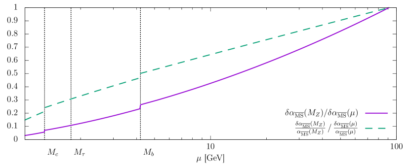
Figure 1: Error of the coupling at a scale $\mu$ compared with the error propagated to the reference scale $M_{Z}$. Note that when the strong coupling is determined at low energy scales the result at the reference scale $M_{Z}$ becomes more precise. For example, the error in $\alpha_{\overline{\rm MS}}(M_{\tau})$ is reduced by almost one order of magnitude when the result is evolved to the scale $M_{Z}$ (solid purple line). This effect is not only due to the reduction in the coupling itself: the relative error in the coupling is reduced approximately by a factor three (dashed green line).

Obtaining a precise value for the strong coupling with high energy experimental input has its own challenges. At high energies the strong coupling is small, which is just what is needed to have the truncation and power corrections under control, but at the same time the effect that one is trying to measure is small. This usually translates in larger uncertainties in $\alpha_{\overline{\rm MS}}(M_{Z})$ from determinations based on data at high energies (see figure 1). Extracting the value of the strong coupling at lower energies usually leads to smaller uncertainties, although the estimation of the truncation uncertainties and the non-perturbative effects become more challenging: clearly the extrapolation $sQ\to\infty$ is more difficult without data at large $Q$.

Another point to take into account is that in contrast with the perturbative computations, quarks are not the observed final states of any physical process. Hadronization and other non-perturbative effects have to be taken into account when comparing experimental data with perturbative predictions, usually by using Monte Carlo generators.

Extraction from data

A well-know example of the extraction of the strong coupling from experimental data is the extraction of $\alpha_{\overline{\rm MS}}(M_{Z})$ using data for $\tau$ decaying into hadrons. We briefly summarise the procedure here, in order to highlight the main steps and the sources of uncertainties, we refer the reader to an extensive review like e.g. Ref. [25] for a detailed discussion. The physical processes considered in this case are the decays of $\tau$ leptons. More specifically, the ratio of the hadronic and leptonic decay widths can be written as

$$R_{\tau,V+A}=\frac{\Gamma(\tau\to\nu_{\tau}+\text{hadrons})}{\Gamma(\tau\to\nu_{\tau}e^{-}\bar{\nu}_{e})}=3|V_{ud}|^{2}S_{\rm EW}\left(1+\delta_{P}+\delta_{\rm NP}\right)\,.$$ (37)

In this case the typical energy scale of the process is set by the $\tau$ mass $Q=M_{\tau}=1.77682(16)$ GeV. In Eq. (37) $S_{\rm EW}(Q)$ is the electroweak contribution to $R_{\tau,V+A}$, and $\delta_{\rm P},\delta_{\rm NP}$ are the QCD perturbative and non-perturbative corrections to the process respectively. The non-perturbative (i.e. power) corrections are estimated to be very small $\delta_{\rm NP}\sim 10^{-4}$ [25]. On the other hand the perturbative prediction

$$\delta_{\rm P}=\sum_{k=1}^{4}r_{n}(s)\,\left(\frac{\alpha_{\overline{\rm MS}}(\mu)}{\pi}\right)^{k}+\mathcal{O}(\alpha_{\overline{\rm MS}}^{5})\,,\qquad(s=\mu/M_{\tau})\,.$$ (38)

is known up to four loops [26, 27, 28]. The impressive perturbative knowledge in the ratio $R_{\tau,V+A}$ makes this quantity a good candidate to determine $\alpha_{\overline{\rm MS}}$. In fact such determinations are one of the most precise phenomenological determinations. On the other hand the scale at which $\alpha_{\overline{\rm MS}}$ is determined is relatively low, and it cannot be changed, since $M_{\tau}$ is what it is.

The procedure with other observables is basically the same, although some details, like the number of known terms in the perturbative expansion or the size of the non-perturbative effects (i.e. $\delta_{\rm NP}$ in Eq. (37)), change from one observable to another.

Combining multiple collider observables in a global fit provides a better lever-arm to constrain $\alpha_{s}$ together with the parton distribution functions (PDFs). Global fits that include the wider ranges of data provide determinations of the strong coupling constant with good statistical accuracy, see e.g.Refs. [29, 30, 31]. The challenges here stem from controlling the systematic errors (both theoretical and experimental) in fits that involve very large and diverse datasets and the relatively low energies involved (see for example the recent review[32]). Moreover, as recently discussed in Ref. [33], determinations of the strong coupling from hadronic processes should entail a simultaneous determination of the parton distribution functions.

Extraction from lattice simulations

Lattice QCD offers an interesting alternative to phenomenological determinations. Being a non-perturbative formulation of QCD, one can combine input from well-measured QCD quantities – like for example the proton mass, or a meson decay constant – with the perturbative expansion of a short distance observable that does not need to be directly observable (like the quark anti-quark force). The advantage of this approach is that the experimental input comes from the hadron spectrum with a negligible uncertainty. Hadronization corrections are not needed, since we are working directly in a non-perturbative framework.

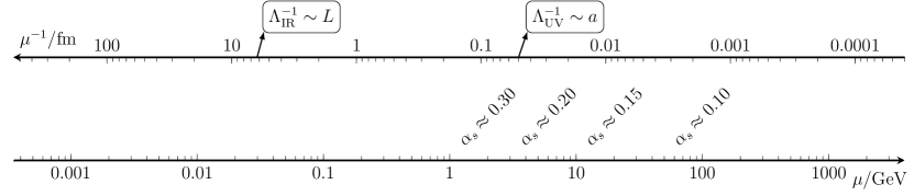
Figure 2: Scales in a typical state of the art lattice computation. The volume of the simulation is a few fm, while the cutoff $1/a$ is a few GeV. Lattice QCD can resolve observables in this window of scales, where the strong coupling is $\alpha_{\overline{\rm MS}}\sim 0.25$.

Despite being very different approaches, both the phenomenological and the lattice QCD methods have to overcome similar challenges. Lattice extractions of the strong coupling must be done at sufficiently high energies so that truncation and power corrections are well under control when matching to perturbative expansions. Due to the finite nature of computer resources, every lattice QCD simulation has two intrinsic scales: the total physical volume simulated $L$ (IR cutoff), usually of a few fermi in order to keep finite-volume corrections well under control, and the lattice spacing $a$ (the UV cutoff $\sim 0.04$ fm in the most challenging present day simulations, which corresponds roughly to a cutoff of 5 Gev in energies). Any lattice QCD simulation can only resolve a process if it is defined at a scale between these IR and UV cutoffs (see figure 2). The number of lattice points in each direction is given by the ratio $L/a$, viz. the separation of the UV and IR cutoffs determines the memory footprint and computing power, and hence the computational cost, of the corresponding simulations, putting in practice a limit on the energy scales that can be studied in any lattice simulation. While in principle lattice techniques can be used to compute non-perturbatively the running of the coupling until the perturbative regime is reached, in practice the range of scales that can be studied in a single lattice simulation is limited by computer resources. Reaching scales higher than a few GeV requires a dedicated approach.

3.2 Systematics in the extraction of $\alpha_{\overline{\rm MS}}$

The truncation performed in Eq. (36) neglects higher order terms (i.e. perturbative corrections) and non-perturbative power corrections. When performing an extrapolation to $Q\to\infty$, these effects only affect how fast we approach the extrapolated value. An example of this behaviour can be seen in figure 3, where different observables (labeled by $\nu$) are used to estimate $\Lambda_{\overline{\rm MS}}$ by matching with perturbation theory at different physical scales $Q$, which are translated in different values of $\alpha_{\overline{\rm MS}}$ in the plot. Different observables predict compatible results for $\Lambda_{\overline{\rm MS}}$ when the extrapolation $Q\to\infty$, corresponding to $\alpha\to 0$ in the plot, is performed. The results of these extrapolations agree well within errors with the result quoted in Ref. [34] (gray error band in the plot). Note however that some observables (it viz.  $\nu=-0.5$) show a slow approach to the extrapolated value, with significant discrepancies even at energy scales $Q\sim 8-10$ GeV.

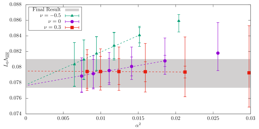
Figure 3: Determination of the $\Lambda$-parameter in units of a scale $L_{0}\sim 1/(4{\rm GeV})$. Different values of $\nu$ represent different choices of observable, and each point corresponds to a determination of the dimensionless product $\Lambda_{\overline{\rm MS}}L_{0}$ using a perturbative expansion (like Eq. (36)). The horizontal axes label the scale of matching with perturbation theory ($\mu$ in Eq. (36)) parametrized in terms of the leading corrections $\mathcal{O}(\alpha_{\overline{\rm MS}}^{2}(\mu))$. The first error bar shows the statistical uncertainty. The second error bar shows the total systematic plus statistic added in quadratures. The systematic uncertainty is determined by varying the renormalization scale a factor of two above and below some specific value. For $\nu=-0.5$ the systematic uncertainty determined with this method is unable to account for the difference with the final results at values of $\alpha\sim 0.13-0.2$, while in other cases ($\nu=0.3$) the systematic uncertainty overestimates the true difference. See text for more details. (source [34, 35]).

In practice performing the extrapolation $Q\to\infty$ is very difficult. Data over a large range of energy scales is required in order to perform such an analysis. For example the data in figure 3 involves precise lattice determinations of the target observables for energy scales $Q\in 2-140$ GeV. This is only possible with a dedicated approach (see section 6.7).

How do we estimate the systematics effects in the extraction of $\alpha_{\overline{\rm MS}}$ when the data does not allow an extrapolation $Q\to\infty$? Of course this is a complex subject in itself, that is of much relevance not only for the extraction of $\alpha_{\overline{\rm MS}}$, but also in the interpretation of many experimental data from hadron colliders. A possible estimate of the uncertainty due to the missing terms is given by the last known term in the series $c_{n}(s)\alpha_{\overline{\rm MS}}^{n}(\mu)$. Generally this results in significant theoretical uncertainties, and, perhaps more interestingly, correlations between experimental data.

A common approach to estimate these uncertaintites exploits the fact that the truncated perturbative expansion to $n^{\rm th}$ order

$$P^{(n)}(Q,s)=\sum_{k}^{n}c_{k}(s)\alpha_{\overline{\rm MS}}^{k}(\mu)\,,\qquad(s=\mu/Q)\,.$$ (39)

still depends on $\mu$, while the true value of the observable $P(Q)$ does not. The truncation of the perturbative expansion introduces a spurious dependence on the renormalization scale, which is in general an unphysical, arbitrary quantity. Higher-order effects are estimated by looking at the variation of $P^{(n)}(Q,s)$ when the renormalization scale $\mu$ is changed by a factor two around some preferred value (for example $\mu=Q$). In principle the relation between a variation in the renormalization scale $\mu$ and the size of the missing higher-order terms given by $\delta_{n}=|P(Q)-P^{(n)}(Q,s)|$ is unclear, beyond the fact that the scale dependence in Eq. (39) is due to the truncation of the perturbative expansion. Under some assumptions on the size of the coefficients of the perturbative expansion ($c_{n+2}(s)\alpha(\mu)\ll c_{n+1}(s)$), it is possible to show that the scale variation yields a sensible estimate of $\delta_{n}$ (see for example Ref. [36]). Formally,

$$\mu\frac{{\rm d}P^{(n)}(Q,s)}{{\rm d}\mu}\propto\alpha_{\overline{\rm MS}}^{n+1}(\mu)\,,$$ (40)

which implies that, at least parametrically, changes in $\mu$ capture the correct size of the missing terms. As an example, a recent comprehensive study of the theoretical uncertainties for numerous observables, based on scale variations, can be found in Refs. [37, 38].

What about power corrections? they are not captured by this kind of analysis. Estimating them requires to have access to different physical scales $Q$. Ideally one would like to work at sufficiently high energies so that they are negligible compared with the accuracy of the data. In practice this is not always the case. Note that the perturbative running is logarithmic, and distinguishing this perturbative running from a power-like behaviour requires data that span large energy ranges.

The assumptions that underlie the scale variation procedure constrain both the non-perturbative effects and the character of the perturbative series. In particular, the assumption that the first unknown term of the perturbative series is smaller than the last known one is implicit in any estimate that uses Eq. (40). Also the value of $\alpha_{\overline{\rm MS}}(\mu)$ is assumed to be small enough so that these uncertainties are meaningful. These assumptions might seem reasonable and mild, and often yield sensible estimates, but there are examples in the literature where they have been shown not to be accurate. Let us mention here three relevant cases.

• The convergence of the perturbative series in practice is not as good as we would like. Due to the asymptotic nature of the PT series, one expects that at some point the coefficients in the perturbative series will grow factorially, see Ref. [39] for a review.

• Extractions of the strong coupling from $\tau$ decays can be done by applying two frameworks in perturbation theory, called fixed order perturbation theory (FOPT) and contour improved perturbation theory (CIPT). Using $\alpha_{\overline{\rm MS}}(m_{\tau})=0.34$ as the typical value of the strong coupling at the scale set by the mass of the $\tau$, the contributions to both perturbative series look as follows

  $$\delta_{\rm FOPT} = 0.1082+0.0609+0.0334+0.0174+0.0087=0.2286\,,$$ (42)

  $$\delta_{\rm CIPT} = 0.1479+0.0297+0.0122+0.0086+0.0037=0.2021\,.$$ (43)

  The terms in both series decrease, and each of the expansions by themselves seem reasonable. Taking the last term as a measure of the uncertainty in the truncation, these values should be accurate with a precision $\sim 0.01$. But both approaches result in values that differ by more than twice this amount. What is more worrisome, for the highest orders the difference between both estimates grows as more terms are included in the expansion.

• The scale variation approach to estimate truncation uncertainties (changing the value of the renormalization scale $\mu$ by a factor two around a preferred value) has been compared with non-perturbative data in a careful study for values of $\alpha_{\overline{\rm MS}}\sim 0.1-0.2$ [35] (see figure 3). The error bars in figure 3 include an estimate of the truncation uncertainty using this approach. It is clear from the plot that for $\nu=-0.5$ the scale variation underestimates the systematic error. Note that the known terms in the perturbative series for all these observables suggest an apparent good perturbative behavior.

These examples show that estimating the truncation uncertainties within perturbation theory is difficult. In the absence of a theorem, our attempts to quantify these uncertainties remain exploratory, and caution should be exercised in interpreting the results. One should never forget the asymptotic nature of perturbative series in QCD [40]. Eventually a factorial growth of the size of the terms in the series is expected, which is deeply related to the non-perturbative effects of the theory. Note however that the structure of the corrections have been investigated at length (see e.g. Ref. [39]). It is clear that there are at least two ingredients in the quality of any extraction of the strong coupling.

1. The value of $\alpha_{\overline{\rm MS}}$ at which perturbation theory is used. Non-perturbative (power) corrections decrease very quickly with $\alpha_{\overline{\rm MS}}$. In order to make them negligible one needs to have access to high energy scales, hence, small values of $\alpha_{\overline{\rm MS}}$.

2. The extraction has to be performed over a range of values of $\alpha_{\overline{\rm MS}}$. This allows the unknown terms in the series to vary substantially, so that one can check that indeed they are negligible. A reasonable requirement would be that the first unknown term $\alpha_{\overline{\rm MS}}^{n+1}$ varies significantly, say by a factor four.

These are two criteria that are usually relevant in any extrapolation. As shown in the examples above, they will impact the quality of any extraction of the strong coupling. Of course some determinations cannot really change the value of the momentum scale at which perturbation theory is used. A good example is the above mentioned extraction from $\tau$ decays, since the mass of the $\tau$ is what it is and sets the overall energy scale to the process. For the case of lattice simulations, changing the values of $\alpha_{\overline{\rm MS}}$ at which perturbation theory is used is challenging, yet feasible. We shall keep these two criteria in mind when describing any lattice computation/method, and not only the quoted theoretical uncertainties.

We would like to end this section recommending the reader the recent contribution to the Lattice Field Theory Symposium by M. Dalla Brida [41], where these issues are also discussed in detail.

4 Lattice field theory

This section summarizes, briefly, the ideas that underlie lattice QCD. While it does not provide an extensive discussion of lattice QCD, it is intended to present the framework of lattice simulations for the non-expert reader in a self-consistent form, setting the notation for the following sections, and providing references for further reading. Hoperfully it will yield the foundations to better understand the sources of systematic errors that are discussed in what follows. It can safely be skipped unless the reader is actually interested in the details of the lattice simulations.

The formulation on a discretized lattice provides a non-perturbative definition of a Quantum Field Theory (QFT). The starting point is the path integral of the theory in Euclidean space

$$\mathcal{Z}=\int\mathcal{D}\bar{\psi}\mathcal{D}\psi\mathcal{D}A_{\mu}\,e^{-S_{\rm QCD}[\bar{\psi},\psi,A_{\mu}]}\,.$$ (44)

where

$$S_{\rm QCD}[\bar{\psi},\psi,A_{\mu}]=\int{\rm d}^{4}x\,\left\{-\frac{1}{2g^{2}}{\rm T\textordmasculine r}\{F_{\mu\nu}F_{\mu\nu}\}+\sum_{f=1}^{N_{\rm f}}\bar{\psi}_{f}(D_{\mu}\gamma_{u}+m_{f})\psi\right\}$$ (45)

Lattice field theory gives a precise definition to the path integral in Eq. (44) by discretizing the spacetime in a hyper-cubic lattice with spacing $a$. In this approach matter fields are defined at the lattice sites $x_{\mu}=an_{\mu}$ for $n_{\mu}=1,\dots,L_{\mu}/a$, where $L_{\mu}$ is the physical size in direction $\mu$. After this discretization the path integral Eq. (44) is simply an integral over very many degrees of freedom (the value of each of the fields at each spacetime point). For example the measure for the fermion fields becomes

$$\mathcal{D}\bar{\psi}(x) \longrightarrow \prod_{n_{\mu}=1}^{L_{\mu}/a}d\bar{\psi}(an_{\mu})\,,$$ (46)

$$\mathcal{D}\psi(x) \longrightarrow \prod_{n_{\mu}=1}^{L_{\mu}/a}d\psi(an_{\mu})\,.$$ (47)

As already discussed the lattice spacing $a$, provides the UV cutoff of the theory.

The most appealing characteristic of the lattice formulation of QCD is that it allows quantitative computations to be performed using numerical simulations. Field correlators are computed as integrals in spaces of very large (but finite) dimensions using Monte Carlo techniques.

A crucial step in lattice field theory consists in defining a “discretized” version of the continuum action $S_{\rm QCD}$. When constructing lattice actions, one has to pay special attention to the symmetries of the theory. Ideally the lattice action should preserve exactly as many of the symmetries of the continuum action as possible. The case of gauge symmetry plays a special role, since it is crucial to guarantee the renormalizability of the theory. Another common requirement for the lattice action is to reduce to the continuum action in the naive classical limit $a\to 0$.

4.1 Gauge fields on the lattice

A naive discretization of the pure gauge action, obtained by substituting the derivatives in the continuum action by finite differences, results in discretization effects that break gauge invariance. The way to construct lattice actions for gauge theories is rooted in the geometric interpretation of gauge invariance, and was first proposed by Wilson [43]. Since the gauge field acts as an affine connection in the continuum theory, its lattice counterpart is the parallel transporter along the links of discretized spacetime. Hence the key idea is to work with link variables

$$U(x,\mu)=e^{aA_{\mu}(x)}\,,$$ (48)

where the pair $(x,\mu)$ uniquely identifies the link that originates from point $x$ in the positive $\mu$ direction. These link variables can be seen as a discretization of a continuum Wilson line, the parallel transporter mentioned above, linking the points $x$ and $x+a\hat{\mu}$ 

$$U(x,\mu)=\mathcal{P}\exp\left\{a\int_{0}^{1}{\rm d}t\,A_{\mu}(\gamma(t))\right\}+\mathcal{O}(a^{2})\,.$$ (49)

Here $\gamma(t)$ is a path that links the point $x$ with $x+a\hat{\mu}$, e.g.

$$\gamma(t)=x+at\hat{\mu}\,,\quad t\in[0,1]\,.$$ (50)

A product of link variables along a closed loop is called a Wilson loop.

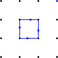
(a) $\mathcal{S}_{0}$

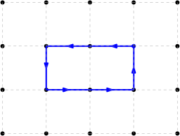
(b) $\mathcal{S}_{1}$

Figure 4: Traces of the plaquette ($\mathcal{S}_{0}$) and the $2\times 1$ Wilson loops ($\mathcal{S}_{1}$) can be used to construct different lattice actions.

Link variables transform under a gauge transformation $\omega(x)\in SU(3)$ as

$$U(x,\mu)\to\omega(x)U(x,\mu)\omega(x+a\hat{\mu})^{\dagger}\,,$$ (51)

which implies that the trace of a Wilson loop is gauge invariant. Lattice actions are constructed by combining these traces, with different choices yielding the same low-energy physics (compared to the cutoff scale), with different lattice artefacts. The simplest choice, first proposed by Wilson, consists in using the smallest possible loop (the plaquette)

$$S_{W}=\frac{1}{g_{0}^{2}}\sum_{\mathcal{W}\in\mathcal{S}_{0}}{\rm tr}\{1-U(\mathcal{W})\}\,,$$ (52)

where the sum runs over all oriented Wilson loops of type $\mathcal{S}_{0}$ (see figure 4). It is easy to check that for a given plaquette $\mathcal{W}_{x}$ in the $\mu,\nu$ plane with left lower corner at point $x$, we have

$${\rm Re}\,{\rm tr}\{1-U(\mathcal{W}_{x})\}=\frac{1}{2}a^{4}{\rm tr}\{F_{\mu\nu}(x)F_{\mu\nu}(x)\}+\mathcal{O}(a^{5})$$ (53)

And therefore the Wilson action reduces to the continuum YM action in the naive limit $a\to 0$.

Improved actions

This is not the only option. By including in the definition of the lattice action larger loops the rate of convergence to the continuum can be improved, i.e. the size of lattice artefacts can be reduced. This is a general programme that goes under the name of improvement, and extends to the fermionic part of the action. Improved actions play an important role in reducing lattice artefacts and therefore providing more precise extrapolations to the continuum limit. Although the literature covers a wide range of lattice actions, most lattice simulations are performed using some particular choice of the one-parameter family that can be constructed from the plaquette and the $2\times 1$ loops (see figure 4)

$$S_{\rm latt}=\frac{1}{g_{0}^{2}}\sum_{i=0,1}c_{i}\sum_{\mathcal{W}\in\mathcal{S}_{i}}{\rm tr}\{1-U(\mathcal{W})\}\,.$$ (54)

The constants $c_{0},c_{1}$ have to obey the constraint

$$c_{0}+8c_{1}=1\,,$$ (55)

in order to recover the classical continuum limit, but otherwise can be chosen at will. Clearly the simple Wilson action, $S_{W}$ in Eq. (52), is recovered by choosing $c_{0}=1,c_{1}=0$. Other popular choices include the Symanzik tree-level improved action ($c_{0}=5/3,c_{1}=-1/12$), or the Iwasaki action ($c_{0}=3.648,c_{1}=-0.331$). A detailed discussion of the improvement of lattice actions is beyond the scope of this review. However the reader should keep in mind that there are discretization effects when reading the lattice literature. These discretization effects induce a systematic error in the lattice observables, which in turn impacts on the determination of the strong coupling. We shall return to this issue later in this paper, when discussing the different lattice extractions of $\alpha$.

For the path integral to be fully specified, it is also necessary to define the integration measure of the gauge link variables $U_{\mu}(x)$. In order to ensure the gauge invariance of the path integral, the measure ${\rm d}U$ of each link variable needs to be invariant under both left and right multiplication by elements of the group:

$${\mathrm{d}}U=\mathrm{d}(gU)=\mathrm{d}(Ug)\,,$$ (56)

where $g$ is a generic element of the gauge group. Imposing the normalization condition

$$\int dU=1\,,$$ (57)

the integration measure is uniquely defined to be the Haar measure on the group. The reader interested in more details can consult any standard reference on compact topological groups. When integrating over all the lattice link variables, we will use the shorthand notation

$${\rm d}U=\prod_{x,\mu}{\rm d}U(x,\mu)\,.$$ (58)

4.2 Fermions on the lattice

4.2.1 Fermionic Path Integral

Fermions in the functional integral language are represented by Grassmann (anti-commuting) variables

$$\{\psi_{i},\psi_{j}\}=\{\psi_{i},\bar{\psi}_{j}\}=\{\bar{\psi}_{i},\bar{\psi}_{j}\}=0\,.$$ (59)

Obviously $\psi_{i}^{2}=\bar{\psi}_{i}^{2}=0$, so that any function of Grassmann variables is defined by its Taylor expansion up to second order. Integrals over Grassmann variables are defined by

$$\begin{split}\int\,{\rm d}\psi=\int\,{\rm d}\bar{\psi}=0\,,\\ \int\,{\rm d}\psi\psi=\int\,{\rm d}\bar{\psi}\bar{\psi}=1\,,\\ \end{split}$$ (60)

Computing integrals of a function of Grassmann variables $f(\psi,\bar{\psi})$ is therefore a problem in combinatorics. When computing the integral over several Grassmann variables we will use the shorthand notation

$${\rm d}\psi=\prod_{i}{\rm d}\psi_{i}\,,\qquad{\rm d}\bar{\psi}=\prod_{i}{\rm d}\bar{\psi}_{i}\,.$$ (61)

A key role is played by the integrals

$$\int{\rm d}\psi{\rm d}\bar{\psi}\,e^{-\bar{\psi}_{i}M_{ij}\psi_{j}} = (-1)^{\frac{n(n-1)}{2}}\det M\,,$$ (62)

$$\int{\rm d}\psi{\rm d}\bar{\psi}\,\psi_{k_{1}}\psi_{k_{2}}\cdots\bar{\psi}_{l_{1}}\bar{\psi}_{l_{2}}\cdots e^{-\bar{\psi}_{i}M_{ij}\psi_{j}} = \sum_{P}(-1)^{\sigma_{P}}(M^{-1})_{k_{a_{1}}l_{b_{1}}}\cdots(M^{-1})_{k_{a_{2}}l_{b_{2}}}$$

with the sum is over all permutation of the $k,l$ indices.

As discussed above, matter fields on the lattice are associated to sites, denoted by the suffices in the equations above. The fermionic action is quadratic in the fermion fields, and different discretizations can be cast into different choices for the matrix $M$. A discretized version of the derivative

$$\partial_{\mu}f(x)=\frac{f(x+a\hat{\mu})-f(x)}{a}\,,$$ (63)

$$\partial_{\mu}^{*}f(x)=\frac{f(x)-f(x-a\hat{\mu})}{a}\,,$$ (64)

enters in the non-diagonal elements of this matrix $M$. Moreover, for fermions minimally coupled to the gauge field, the discrtized derivative needs to be replaced by its covariant version. Hence in QCD the matrix $M$ depends on the gauge field configuration $U_{\mu}(x)$ and the mass of the fermions $m_{\mathrm{f}}$. We will use the notation

$$D_{\mathrm{f}}=D\left[U,m_{\mathrm{f}}\right]\,,$$ (65)

to denote the lattice Dirac operator for one fermion species, the latter being identified by the index $\mathrm{f}$.

Although the simulation of Grassmann variables on a computer is possible, it is computationally very inefficient. Instead, the previous relation is used to directly define the path integral of lattice QCD as (cf. Eq. (62))

$$\mathcal{Z}=\int{\rm d}U\,\,\left[\prod_{\mathrm{f}=1}^{N_{\rm f}}\det(D_{\rm f})\right]e^{-S_{G}[U]}\,.$$ (66)

Note that by integrating out the fermions fields exactly, one is effectively simulating a non-local theory.

4.2.2 Chiral symmetry and lattice fermions

The Euclidean action for a single free fermion in the continuum reads

$$S_{F}[\psi,\bar{\psi}]=\int{\rm d}^{4}x\,\bar{\psi}(\gamma_{\mu}\partial_{\mu}+m)\psi\,.$$ (67)

A naive attempt to discretize this action leads to the so-called doubling problem: instead of describing a single fermion, the lattice action describes $2^{4}$ fermion flavors. In fact this phenomenon is intimately related with chiral symmetry. In the absence of a mass term the fermion action is invariant under chiral transformations

$$\psi\mapsto e^{\imath\theta\gamma_{5}}\psi\,,\quad\bar{\psi}\mapsto\bar{\psi}e^{\imath\theta\gamma_{5}}\,.$$ (68)

This is just a consequence of the kernel of the fermion bilinear being proportional to $\gamma_{\mu}$. The Nielsen-Ninomiya theorem [44, 45, 46] shows that any local lattice hermitian action that preserves translational invariance and chiral symmetry describes an equal number of positive- and negative-chirality fermions. In the case of the naive fermion action, the Nielsen-Ninomiya theorem is satisfied because of the 16 fermions, 8 have positive chirality and the remaining 8 have negative chirality. It is possible to reduce the number of doublers from 15 to just 1, but in order to describe a single fermion one has to break one of the hypotheses of the Nielsen-Ninomiya theorem. Giving up locality leads to serious difficulties for the renormalization of the theory. Therefore most efforts have focused on four particular approaches.

Wilson fermions

One of the most popular choices follows Wilson’s original proposal to break chiral symmetry at finite lattice spacing by an irrelevant operator [47]. This is implemented by adding a dimension 5 term to the Lagrangian that is just a suitable discretization of

$$\mathcal{L}_{5}=\frac{r}{2}\bar{\psi}\partial^{2}\psi\,.$$ (69)

The addition of this irrelevant operator has nevertheless an important impact in the spectrum of the theory by removing all the doublers.

There are two unpleasant effects of this extra term in the action. Firstly the fermion mass is no longer protected by chiral symmetry in the regularised theory, and therefore acquires an additive renormalization. As a consequence the massless theory can only be obtained by fine tuning the bare mass in the action. Secondly the scaling violations are linear in the lattice spacing $\mathcal{O}(a)$. The massless theory can be non-perturbatively improved by adding the so called Sheikholeslami-Wohlert term [48]

$$\mathcal{L}^{\prime}_{5}=c_{\rm SW}\bar{\psi}F_{\mu\nu}[\gamma_{\mu},\gamma_{\nu}]\psi\,.$$ (70)

If the coefficient $c_{\rm SW}$ is chosen appropriately (see [49]), all remaining linear cutoff effects are proportional to the quark masses $\mathcal{O}(am)$.  This last term is usually called clover term in the lattice jargon, and the discretization is referred as Wilson-clover fermion action.

Twisted mass fermions

A close relative of Wilson clover fermions are twisted mass fermions. In this case one uses the same 5-dimensional operator to break chiral symmetry, except that in this case the mass term is of the form

$$m+\imath\mu\gamma_{5}\tau_{3}\,,$$ (71)

where $\tau_{3}$ is the third Pauli matrix acting in flavor space. Twisted mass lattice QCD always describes multiples of two fermion flavors with a mass given by a combination of $m$ and $\tau$. Note that in the continuum one can always set $\mu=0$ (with the help of a non-anomalous chiral transformation), recovering the usual mass term.

On the other hand, at non-zero values of the lattice spacing, the twisted mass term cannot be reduced to the standard Wilson form, because of the explicit breaking of chiral symmetry of the Wilson term Eq. (69). The main advantage of this formulation is that, for a specific choice of the mass parameter $m$ (called maximally twisted) all physical observables are automatically $\mathcal{O}(a)$-improved [51]. In twisted mass lattice QCD there is no need of tuning the $c_{\rm SW}$ term of Eq. (70). On the other hand, parity and flavor symmetries are broken at finite lattice spacing, and, as already mentioned, one can only simulate an even number of quarks. The reader might be interested in the review [52].

Staggered fermions

One can live with some of the doublers and in fact use them in one’s favor [53, 54]. This is the approach taken by the staggered formulations of QCD: some of the doublers are used to represent the 4 spin components of the fermion. The staggered fermion formulation therefore reduces the amount of doublers to 4. The main advantage of this approach is that it preserves an exact $U(1)$ symmetry that is enough to guarantee, among other things, that scaling violations are proportional to $a^{2}$. Moreover they are computationally cheap.

The main drawback of this particular fermion formulation is that the 4 remaining doublers are degenerate in mass, while the 4 lightest quarks in nature have very different masses. In order to describe single flavors, the staggered fermion formulation uses a rooting prescription: the fermion determinant that describes the 4 doublers is replaced with its fourth root with the hope that this will describe a single flavor [55]. This rooting prescription has the unpleasant effect of breaking locality. It has been argued that locality is recovered in the continuum. If this is actually the case or not has been the subject of many heated discussions in the past, although the issue has never been completely resolved [56, 57, 58, 59].

Domain Wall fermions

One way to circumvent the Nielsen-Ninomiya theorem is to require that the fermion action, at finite lattice spacing, is invariant under a set of modified chiral transformations,

$$\psi\mapsto e^{i\alpha\gamma_{5}[1-2\zeta aD]}\psi\,,\quad\mathrm{and}\ \quad\bar{\psi}\mapsto\bar{\psi}e^{i\alpha\gamma_{5}[1-2(1-\zeta)aD]}\,,$$ (72)

where $\zeta$ is a free parameter [60]. A lattice Dirac operator that is invariant under these transformation satisfies

$$\left\{\gamma_{5},D\right\}=2aD\gamma_{5}D\,.$$ (73)

This relation is known as Ginsparg-Wilson relation, and was derived from renormalization group arguments in Ref. [61] long before the symmetry above was suggested.

One solution of Eq. (73) is the overlap operator obtained in Ref. [62]:

$$aD_{N}=\frac{1}{2}\left[1+\gamma_{5}\mathrm{sgn}\left(H\right)\right]\,,$$ (74)

where $H=\gamma_{5}(D_{W}-M)$, where $D_{W}$ is a lattice Dirac operator that has the correct naive continuum limit, and $M\sim 1/a$ is a mass parameter.

The operator $D_{N}$ is a representation in terms of four-dimensional fields of five-dimensional domain-wall fermions (DWF) [63]. In DWF formulations, a fermionic zero-mode with definite chirality, localised on the boundary of the (semi-infinite) extra dimension, plays the role of a four-dimensional chiral fermion, while the other states decouple from the low-energy dynamics. As it turns out, the five-dimensional formulations of DWFs presented in Refs. [64, 65] has become the method of choice for simulating chiral fermions on the lattice. Without entering into a detailed explanation of the DWF construction on the lattice, we write down explicitly the action for DWF, and discuss some of its features, while referring the interested reader to the literature for detailed discussions [66, 67]. Denoting the coordinate in the fitfth direction by $s\in[0,\infty)$, the DWF action in Ref. [64] reads

$$S= \sum_{x,s,\mu}\bar{\psi}(x,s)\gamma_{\mu}\partial_{\mu}\psi(x,s)+M\bar{\psi}(x,s)\psi(x,s)+\frac{r}{2}\sum_{x,s,\mu}\bar{\psi}(x,s)\partial_{\mu}^{2}\psi(x,s)\,+$$

$$+\sum_{x,s>0}\bar{\psi}(x,s)\gamma_{5}\partial_{5}\psi(x,s)+\frac{r}{2}\sum_{x,s>0}\bar{\psi}(x,s)\partial_{5}^{2}\psi(x,s)\,+$$

$$+\frac{1}{2}\sum_{x}\bar{\psi}(x,0)\gamma_{5}\psi(x,1)+\frac{r}{2}\sum_{x}\bar{\psi}(x,0)\left[\psi(x,1)-2\psi(x,0)\right]\,.$$ (75)

The index $\mu$ runs over the first four Euclidean directions, and the derivatives $\partial_{\mu}$ become covariant derivatives when the fermions are coupled to a four-dimensional gauge field. In actual simulations the fifth dimension has a finite size, while the lattice chiral symmetry is only recovered when the size of the fifth dimension goes to infinity. In practice a balance must be found between the breaking of chirality due to the finite fifth dimension and the growing cost of the simulations as the size of this dimension is increased.

4.3 Masses, correlators and all that

Quantum Field Theories provide the machinery to evaluate field correlators, i.e. the expectation value of functions of the elementary fields that appear in the definition of the path integral. Specific physical properties can then be extracted from these correlators by means of dedicated analyses. It is interesting to discuss a few explicit examples in order to introduce some of the quantities that are used later in this review.

Let us begin with a two-point correlator

$$C_{\Gamma\Gamma^{\prime}}(t)=\sum_{\mathbf{x},\mathbf{y}}\langle O_{\Gamma}(t,\mathbf{x})\,O_{\Gamma^{\prime}}^{\dagger}(t,\mathbf{y})\rangle\,,$$ (76)

where $O_{\Gamma}$ is a quark bilinear

$$O_{\Gamma}(t,\mathbf{x})=\bar{q}(t,\mathbf{x})\Gamma q^{\prime}(t,\mathbf{x})\,.$$ (77)

The matrix $\Gamma$ determines the spin structure of the bilinear, which we assume to be a color singlet. In Eq. (77) we have suppressed the flavor indices, for simplicity, we assume the bilinear to be a non-singlet with respect to flavor transformations.

Using Wick’s theorem, the correlator can be rewritten in terms of quark propagators:

$$C_{\Gamma\Gamma^{\prime}}(t)=\sum_{\mathbf{x},\mathbf{y}}\mathrm{tr}\ \left[\Gamma^{\prime}S(0,\mathbf{y};t,\mathbf{x})\Gamma S^{\prime}(t,\mathbf{x};0,\mathbf{y})\right]\,,$$ (78)

where $S(x;y)$ and $S^{\prime}(x,y)$ are the propagators of the quarks $q$ and $q^{\prime}$ respectively, computed as the inverse of the Dirac operator in the gauge background. The expectation value is computed by averaging the trace above over an ensemble of gauge configurations generated by Monte Carlo methods.

In order to extract physical quantities from a two-point function, we insert a complete set of hadronic states,

$$1=\sum_{n}\int\frac{d^{3}\mathbf{p}}{(2\pi)^{3}}\frac{1}{2E_{n}}|n,\mathbf{p}\rangle\langle n,\mathbf{p}|\,.$$ (79)

A few lines of algebra show that the sum over the spatial coordinates implements a projection over zero-momentum states, and therefore

$$C_{\Gamma\Gamma^{\prime}}(t)=\sum_{n}\frac{1}{2E_{n}}\,\langle 0|O_{\Gamma}(0)|n,{\mathbf{p}}=0\rangle\langle n,{\mathbf{p}}=0|O_{\Gamma^{\prime}}(0)^{\dagger}|0\rangle e^{-E_{n}t}\,.$$ (80)

The two-point function can be trivially extended to project on eigenstates of the spatial momentum.

Eq. (80) shows the main features that allow the extraction of physical observables from field correlators. In Euclidean space the time dependence of correlators is a sum of exponentials, whose decay rates are determined by the energies of the states that have a non-vanishing matrix element $\langle 0|O_{\Gamma}(0)|n,{\mathbf{p}}=0\rangle$. For this reason these operators are often called interpolating operators. For large time separations, the correlators are dominated by the lowest energy state, and the time dependence becomes a simple exponential. The prefactors multiplying the exponential yield various combinations of matrix elements of interest.

The so-called effective mass is defined as the time-derivative of the two-point function:

$$M_{\mathrm{eff}}(t)=-\frac{d}{dt}\log C_{\Gamma\Gamma^{\prime}}(t)=E_{0}+c\,e^{-(E_{1}-E_{0})t}+\ldots\,.$$ (81)

For large times $t$, $M_{\mathrm{eff}}(t)$ tends to a constant, which is the mass of lowest-energy state. However for the range of separations that can be achieved in practice, it is always important to check that the contamination from excited states is sufficiently small, or otherwise under control, since this is one of sources of systematic error that affect the computation of physically interesting observables.

Another interesting example is the computation of the PCAC mass. Specialising the above interpolating operators to the case of two degenerate light quarks ($u$ and $d$), and following the notation in Ref. [68], we define

$$P^{ud}(x)=\bar{u}(x)\gamma_{5}d(x)\,,\quad\mathrm{and}\quad A^{ud}_{\mu}(x)=\bar{u}(x)\gamma_{\mu}\gamma_{5}d(x)\,,$$ (82)

and the two-point correlators

$$C_{PP}(t) =\sum_{\mathbf{x}}\langle P^{ud}(t,\mathbf{x})P^{du}(0)\rangle\,,$$ (83)

$$C_{AP}(t) =\sum_{\mathbf{x}}\langle A^{ud}_{0}(t,\mathbf{x})P^{du}(0)\rangle\,.$$ (84)

Following the arguments above, $C_{PP}(t)$ at large distances is dominated by a a single pseudoscalar state. Denoting by $M_{\mathrm{PS}}$ the mass of the pseudoscalar state, and by $G_{\mathrm{PS}}$ its vacuum-to-meson matrix element, we obtain

$$C_{PP}(t) =-\frac{G_{\mathrm{PS}}^{2}}{M_{\mathrm{PS}}}\,e^{-M_{\mathrm{PS}}t}+\ldots\,.$$ (85)

Interestingly the ratio

$$m_{\mathrm{\tiny PCAC}}=\left(\frac{1}{2}(\partial_{0}+\partial_{0}^{*})C_{AP}(t)+c_{A}a\partial_{0}^{*}\partial_{0}C_{PP}(t)\right)/C_{PP}(t)\,,$$ (86)

tends to the PCAC mass defined in the continuum theory through the axial Ward identity. The interest in the PCAC mass is two-fold. For fermionic formulations that break explicitly chiral symmetry at finite lattice spacing, like e.g. the Wilson fermions described above, the bare parameters in the action need to be tuned to approach the chiral limit. In particular an additive renormalization of the bare fermion mass is required. The chiral theory is defined by requiring the PCAC mass to vanish. After renormalization, the rate of convergence of $m_{\mathrm{\tiny PCAC}}$ will be proportional to the lattice spacing $a$ if the theory is not improved, while it becomes proportional to $a^{2}$ when $c_{\rm SW}$ in Eq. (70) and $c_{A}$ in Eq. (86) are properly tuned.

Note that the decay constant of the PS state, defined as

$$\langle 0|A_{\mu}(0)|\mathrm{PS}\rangle=iZ_{A}F_{\mathrm{PS}}p_{\mu}\,,$$ (87)

can be computed directly from fitting $C_{AP}(t)$ and $C_{PP}(t)$, which yield the matrix elements $\langle 0|A_{0}(0)|\mathrm{PS}\rangle$ and $\langle 0|P(0)|\mathrm{PS}\rangle$. Alternatively, the decay constant can be evaluated from the quantities defined above using

$$F_{\mathrm{PS}}=Z_{m}\frac{m_{\mathrm{\tiny PCAC}}}{M_{\mathrm{PS}}^{2}}\,G_{\mathrm{PS}}\,.$$ (88)

It is interesting to remark that the two definitions differ by lattice artefacts. While in general this is not necessarily a cause for concern, it shows that definitions that are equivalent in the continuum limit do differ at finite lattice spacing. This is something to keep in mind in choosing observables when aiming for high precision measurements.

4.4 Systematic effects in lattice QCD

Any lattice QCD computation has several sources of systematic uncertainties that have to be kept under control in order to be able to quote accurate results. Since lattice QCD is a first principle definition of QCD, these sources of systematic uncertainties reflect the current limitations in computer power, or in our knowledge of efficient algorithms. Since both computer power and our knowledge of efficient algorithms are constantly improving, lattice QCD is able to solve now problems that were basically impossible just a few years ago.

The most basic limitation that computer power sets in any lattice computation is related to the number of points $(L/a)^{3}\times(T/a)$ simulated (the lattice volume). The computer cost increases at least linearly with this lattice volume, and sets a basic compromise between simulating a large physical volume, and a small lattice spacing. Computing resources also limit the range of quark masses that can be simulated, even though it has become common to have simulations with physical quark masses. In summary we have the following main sources of systematic error.

Finite volume corrections:

QCD quantities determined on a large but finite box suffer from finite volume effects. These are exponentially suppressed with the smallest mass present in the spectrum of the theory (i.e. the pion $M_{\pi}$) [70]

$$\propto e^{-M_{\pi}L}\,.$$ (89)

Usually $M_{\pi}L>4$ is sufficient for finite volume effects to be a small sub-percent correction to the quantities determined on a finite volume box. $M_{\pi}L>3$ is the bare minimum to keep these effects under control.

For some hadronic quantities (e.g. meson decay constants) chiral perturbation theory yields an estimate of the size of the finite volume corrections, allowing to subtract them from the data in some cases.

Since one typically uses a short distance observable to determine the strong coupling, these determinations are normally affected very little by finite volume effects. Nevertheless every determination of the strong coupling needs a determination of the scale (see section 4.5.2), where finite volume corrections can be substantial.

Continuum extrapolation:

All determinations on the lattice require a continuum extrapolation to reproduce QCD results. Lattice artefacts are small only if we can achieve a significant separation between the scales at which observables are defined and the lattice cutoff. We will examine in detail the process of taking the continuum limit in section 4.5. Here we just mention that this point is particularly delicate for the determinations of the strong coupling. As we try to use observables computed at high energies in order to define the strong coupling, we necessarily need to face the issue of larger cutoff effects. Typical current large volume simulations use $a\approx 0.04-0.1~{}{\rm fm}$.

Chiral extrapolation:

Many lattice QCD computations used to be performed at nonphysically heavy values of the quark masses. There are two reasons for this. First, lattice QCD simulations become more expensive at lighter quark masses. The gap in the spectrum of the Dirac operator depends on the mass of the lightest quark in the simulation. This has the effect of making simulations close to physical values of the quark masses computationally very expensive. Second, close to physical values for the quark masses finite volume effects are larger, and therefore there is an extra cost due to the need to simulate in larger physical volumes.

For example, simulating physical values for the quark masses ($M_{\pi}\approx 135\,{\rm MeV}$) with sub-percent finite volume effects $M_{\pi}L=4$ and a very fine lattice spacing $a\approx 0.05\,{\rm fm}$ requires a lattice with $L/a\approx 120$ points in each direction. At the time of writing this report this is right at the edge of current capabilities for most choices of lattice action. Algorithmic developments have made it possible to simulate directly at the physical point, but these physical regimes of the parameters are usually simulated on coarser lattices, making the chiral extrapolation a crucial ingredient of any lattice QCD computation.

4.5 The continuum limit and scale setting

Any lattice action has $N_{\rm f}+1$ free parameters: the bare quark masses in lattice units $am_{0}$, and the bare coupling $g_{0}$ (usually the lattice community uses $\beta=6/g_{0}^{2}$ as input parameter for the simulations). While the role of the bare quark masses is clear (they directly affect the values of the quark masses), the role of the bare coupling is less obvious. In fact the bare coupling is tuned in order to approach the continuum limit. Naively the continuum limit amounts to take $a\to 0$. But in the lattice action there is nowhere any reference to the lattice spacing $a$ (or any other parameters with dimensions), raising the question about how to actually take the continuum limit.

Since all lattice input parameters are dimensionless, lattice QCD by itself only gives predictions of dimensionless quantities. For example, the study of the proton correlator yields the proton mass in lattice units $aM_{p}$. The key idea in order to make contact with physical, dimensionful, quantities is to choose one quantity as a reference scale. Every other dimensionful quantity is computed in units of this reference scale. For example, one can take as reference scale the proton mass $M_{p}$. Any other quantity, say for instance the $\Omega$ baryon mass is measured in units of this reference mass – in practice in a lattice simulation we determine the dimensionless ratio $(aM_{\Omega})/(aM_{p})=M_{\Omega}/M_{p}$.

If we focus on the case of $N_{\rm f}=2+1$ simulations (two degenerate light quark masses plus the strange quark), a prediction for the value of $M_{\Omega}$ would conceptually proceed as follows:

1. Choose a value of the bare coupling $g_{0}$. Measure the values of the masses of the $\pi$ and $K$ mesons and the reference scale in lattice units (i.e. $aM_{\pi},aM_{K},aM_{p}$). Tune the bare quark masses such that the ratios of the pseudo goldstone bosons masses to the reference scale $(aM_{\pi})/(aM_{p})$ and $(aM_{K})/(aM_{p})$ are equal to the physical values $M_{\pi}^{\rm exp}/M_{p}^{\rm exp}$ and $M_{k}^{\rm exp}/M_{p}^{\rm exp}$, see e.g. the values reported by the PDG [71]. This procedure fixes the values of the bare quark masses $am_{0}$ for each choice of $g_{0}$. The lattice spacing is then $a=(aM_{p})/M_{p}^{\rm exp}$, where the numerator is the output of the numerical simulation, and the denominator is the reference scale.

2. Repeat the process for several values of $g_{0}$. The final prediction has to be taken as the limit where the reference scale in lattice units is much smaller than one, i.e. $aM_{p}\ll 1$:

   $$\frac{M_{\Omega}}{M_{p}}=\lim_{aM_{p}\to 0}\frac{aM_{\Omega}}{aM_{p}}\,.$$ (90)

   By using the experimental value of the proton mass $M_{p}\approx 940$ MeV, this last prediction of a dimensionless ratio can be translated in a prediction for $M_{\Omega}$.

The first step sets up a line of constant physics (LCP). It requires one experimental input per quark mass. Pseudo-goldstone bosons are the natural candidates, since their mass depends strongly on the values of quark masses. The value of the reference scale ($M_{p}$ in the example) is an extra input, used to convert lattice dimensionless predictions in dimensionful quantities. Note that although usually one takes the values of the quantities to fix from experiment, one can follow the same procedure to set up a line of constant physics at arbitrary non-physical values of the quark masses (for example to investigate a world with mass degenerate $u,d,s$ quarks): lattice QCD also allows to make unambiguous predictions of dimensionless quantities for unphysical values of the quark masses. The second step takes the continuum limit. Different LCP (for example by choosing a different reference scale) would result in different approaches to the same universal continuum values.

These two steps together define a non-perturbative renormalization scheme for the theory. The bare parameters are tuned in order to reproduce some physical world (values of the quark masses and reference scale) and quantities are computed in the limit where the UV cutoff ($1/a$) is much larger than the energy scales of interest ($M_{p},M_{\Omega},\dots$). Asymptotic freedom can be used as a guidance in order to take this continuum limit. At short distances the theory is weakly coupled, which suggests that a series of decreasing values of the bare coupling $g_{0}$ will successively approach the continuum limit.

Even though the procedure sketched above is perfectly correct from a conceptual point of view, it misses some fine details that are crucial in order to obtain the precision achieved nowadays. Let us briefly mention them here.

• As mentioned above lattice QCD simulations become very expensive at the bare parameters that correspond to the physical values of the quark masses. There are two reasons for this. First is the increasing numerical cost of simulating quarks at small values of the bare quark mass. Second, lighter values of the quark masses result in lighter values of the $\pi$ meson masses. Since $M_{\pi}L$ is the quantity that dictates the size of finite volume effects, simulations at lighter quark masses requires to simulate larger physical volumes. In many practical situations the physical point is only reached by extrapolating from simulations at heavier quark masses, although this situation is changing fast with the increasing computer power and improved simulation algorithms.

• The experimental values of the physical hadronic quantities are affected by the electromagnetic interactions. This has implications for the determination of the LCP, since the use of the experimental values as input for a lattice QCD computation has to be done with care, usually correcting them for isospin breaking effects. One has to make sure that the size of the electromagnetic effects has a negligible effect in the determination of physical quantities. When this is not the case, a first-principles prediction requires to simulate both the strong and the electromagnetic interactions in order to make contact with the physical world. We anticipate here that for the case of the the determination of $\alpha_{s}$, isospin breaking effects are not particularly relevant at the current level of precision (cf. section 7).

4.5.1 Systematics in the continuum extrapolation

Since short-distance observables are more susceptible to show large cutoff effects, the continuum extrapolation plays a key role in the extraction of the strong coupling. Here we want to show in some detail how to asses the quality of these continuum extrapolations.

Most lattice QCD simulations choose an improved discretization where the leading scaling violations that we discussed above are $\mathcal{O}(a^{2})$. This is achieved either by choosing a fermion formulation where any $\mathcal{O}(a)$ violations are forbidden by symmetry arguments (like domain-wall fermions, twisted mass at maximum twist, or staggered fermions), or by tuning the parameters of the action (the so-called Wilson-clover fermions). In this situation any dimensionless quantity $D$ has an asymptotic expansion of the form

$$D\raisebox{-0.43057pt}{ $\stackrel{{\scriptstyle\small{a\to 0}}}{{\sim}}$}D_{\rm cont}+\dots\,,$$ (91)

where the dots represent the scaling violations, with an asymptotic expansion with leading term $\mathcal{O}(a^{2})$. But the functional form of these scaling violations is in general very complicated. The corrections include logarithmic terms of the form (i.e. are of the form $a^{n}\log^{k}a$). How does these generic statements affect in practice the extrapolation of lattice data? It is clear that corrections need to be small in order for the precise functional form to have a negligible effect on the extrapolation.

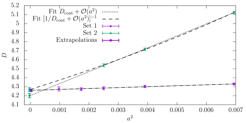
Figure 5: Continuum extrapolation of a dimensionless quantity. Without entering in the details of the definition of the specific quantity in the plot, it is worth noting that these data correspond to actual lattice simulations, see [72] for more details.

In order to be more precise it is best to look at one example. Figure 5 shows the continuum extrapolation of a dimensionless quantity using two different discretizations. These are labeled 1 and 2 respectively in the legend. The extrapolations of both datasets have very different scaling violations, and this has an impact in the accuracy of the continuum value. These differences are:

Range of lattice spacings:

Dataset 1 includes simulations that span a factor

$$a_{\rm max}/a_{\rm min}\approx 2.5$$

in lattice spacings, while dataset 2 has data that span only a factor

$$a_{\rm max}/a_{\rm min}\approx 1.7\,.$$

Size of the extrapolation:

Dataset 1 has very small scaling violations: the finest lattice spacing is compatible within errors with the continuum value. On the other hand dataset 2 shows large scaling violations: the data at the finest lattice spacing is about 5 standard deviations away from the extrapolated value.

These two points are crucial to understand the assumptions that are behind the extrapolation of these two datasets. What we need is a way to measure the impact of the terms beyond the leading $\mathcal{O}(a^{2})$ scaling violations. In order to do so, it is useful to consider not only the extrapolation of $D$, but also the extrapolation of different functions $f(D)$. In principle this function seems completely redundant, since

$$f(D)\raisebox{-0.43057pt}{ $\stackrel{{\scriptstyle\small{a\to 0}}}{{\sim}}$}f_{\rm cont}+\dots\,,\qquad(f_{\rm cont}=f(D_{\rm cont}))\,,$$ (92)

one can, in principle, recover the same $D_{\rm cont}$ from any choice of function by using

$$D_{\rm cont}=f^{-1}(f_{\rm cont})\,.$$ (93)

However, when the range of lattice spacings available is not very large and/or the extrapolation is quite sizable, the choice of function can change substantially the result of the extrapolation. This is illustrated in figure 5, with two simple choices $f(x)=x$ (i.e. extrapolating the data itself) and $f(x)=1/x$ (i.e. extrapolating the inverse of the data). In set 1, these different choices result in practically identical values for the extrapolated value. On the other hand in set 2 the different choices of $f$ result in extrapolations that differ by several standard deviations. Obviously the difference between these two choices for the extrapolation are higher order terms, since

$$\frac{1}{A+Ba^{2}}=\frac{1}{A}-\frac{B}{A^{2}}a^{2}+\frac{B^{2}}{A^{3}}a^{4}+\dots\,.$$ (94)

These results suggest that the dependence of the extrapolation on the choice of function $f$ is equivalent to a dependence on the non-leading scaling violations. It is important to note that discriminating among different functions cannot always be done by looking at the quality of the fit. In the quoted example of figure 5 the fits for the two choice of $f$ are equally good.

Another important point worth mentioning is that this kind of analysis usually only explores the non-leading power corrections (i.e. $a^{4}$ in the example). Logarithmic corrections are much more difficult to estimate, although one should be very careful with neglecting them (the reader interested in this topic will enjoy the puzzle described in Ref. [73], and the recent discussion in the context of lattice QCD [74]). These topics are also very nicely discussed in a recent contribution to the Lattice Field Theory Symposium [41], a reference that we recommend to the reader will enjoy.

Summarising these results, it is crucial to remember that any extrapolation is based on some assumptions. In the case of the continuum extrapolations, these assumptions depend crucially on three characteristics of the dataset: the number of lattice spacings simulated, the ratio of the coarser and the finest lattice spacings, and the size of the extrapolation.

4.5.2 Scale setting in lattice QCD

This process of taking the continuum limit is usually seen by the lattice community from an equivalent perspective, which comes under the name of scale setting. As discussed above some reference scale  $M_{\rm ref}$ is used to determine the value of the lattice spacing $a$. This is simply done by setting up a line of constant physics and declaring that

$$a\equiv\frac{\left(aM_{\rm ref}\right)}{M_{\rm ref}^{\rm exp}}\,,$$ (95)

where the parentheses emphasise that $\left(aM_{\rm ref}\right)$ is the quantity that is actually computed in a lattice simulation, and $M_{\rm ref}^{\rm exp}$ is the experimental value of the reference scale. Now any other quantity $Q$ with units of mass can be determined by the expression

$$Q=\lim_{a\to 0}\frac{(aQ)}{a}\,.$$ (96)

Obviously this is just a rephrasing of Eq. (90). Note that determinations of $a$ are intrinsically entangled with the LCP and the experimental quantity that is used to set the scale (the particular choice of $M_{\rm ref}$). Different LCP and/or physical quantities will result in different values for the lattice spacing. This is however not a problem since any such determinations will give the same predictions for any physical quantity after the continuum limit is taken. This procedure explains the usual jargon of the field: one experimental input is used to determine the lattice spacing.

Scale setting is a key ingredient in any lattice determination of the strong coupling. The $\Lambda$ parameter is a quantity with units of mass, and therefore the error in the scale translates into an equal relative error in the determination of $\Lambda$. What is more important any unaccounted systematic in the determination of the scale propagates into an effect of the same relative size to $\Lambda$. What quantities are used as reference scales? Ideally one would like some quantity that has a clean and precise experimental determination, and that can be determined with high precision and accuracy on the lattice. The reader might be surprised to read that no such clean quantity exist. For example the above mentioned proton mass, that would look as a natural quantity, has a large signal to noise problem (see appendix A), especially close to the physical point. In practice different quantities are used, with each choice having pros and cons. Let us briefly review the characteristics of some of them.

Meson decay constants ($F_{\pi},F_{K}$)

These quantities are clean from a lattice point of view, which explains why they are a popular choice in the lattice community. They are determined from meson 2-point functions, as discussed above. For example $F_{\pi}$ is obtained thanks to the relation

$$\left\langle 0|\bar{u}\gamma_{5}\gamma_{0}d(0)[\bar{u}\gamma_{5}\gamma_{0}d(x)]^{\dagger}|0\right\rangle\sim aM_{\pi}(aF_{\pi})^{2}e^{-aM_{\pi}\,x_{0}}+\dots\,,$$ (97)

which is free from the infamous signal-to-noise problem, leading to these decay constants in lattice units $aF_{\pi},aF_{K}$ being determined with a precision of a few permille. One problem is that the chiral corrections on the decay constants (especially $F_{\pi}$) is not small. Recent determinations are performed at values of the quark masses very close to its physical values, so in principle this has become a lesser issue in state of the art calculations.

On the other hand decay constants are not that clean from the experimental point of view. First, there is a theoretical issue in the definition of these quantities. They are unambiguous in QCD, but the electromagnetic interactions render these quantities ill defined – the quantity in Eq. (97) is not even invariant under a $U(1)$ gauge transformation. The actual experimental observable is the photon-inclusive decay rate $\Gamma_{Pl2}$, defined as

$$\Gamma_{Pl2}=\Gamma(P\rightarrow l\nu)+\Gamma(P\rightarrow l\nu\gamma)\,,$$ (98)

with $P=K^{\pm},\pi^{\pm}$. Most lattice QCD calculations  compute the isospin symmetric quantity $F_{P}$ which parametrizes the decay of the pseudoscalar in a world where electromagnetic interactions are switched off, and isospin is unbroken:

$$\Gamma(P\rightarrow l\nu)\Big{|}_{\alpha_{\rm EM}=0,m_{u}=m_{d}}=\frac{G_{F}|V_{P}|^{2}F_{P}^{2}}{4\pi}\,M_{P}m_{l}^{2}\left[1-\frac{m_{l}^{2}}{M_{P}^{2}}\right]^{2}\,.$$ (99)

In order to relate these two quantities we need to estimate the EM effects. The master formula, as discussed in Ref. [75], is

$$\Gamma_{Pl2}=\Gamma(P\rightarrow l\nu) \times \left[1+\delta_{\rm EW}\right]\times\left(1+\delta_{\rm EM}^{P}\right)\,,$$ (100)

where the first bracket term is the universal electroweak correction

$$\delta_{\rm EW}=0.0232\approx\frac{2\alpha_{\rm EM}}{\pi}\log\left(\frac{m_{Z}}{m_{\rho}}\right)\,,$$ (101)

a short distance contributions that affects all semileptonic charged current amplitudes when expressed in terms of the Fermi constant. Finally the $\delta_{\rm EM}^{P}$ piece can be written as

$$\begin{split}\delta_{\rm EM}^{P}=-\frac{\alpha_{\rm EM}}{\pi}&\left\{-F\left(\frac{m_{l}^{2}}{m_{P}^{2}}\right)+\frac{3}{2}\log\left(\frac{m_{\rho}}{m_{P}}\right)+c_{1}^{P}\right.\\ &+\left.\frac{m_{l}^{2}}{m_{\rho}^{2}}\left[c_{2}^{P}\log\left(\frac{m_{\rho}}{m_{l}}\right)+c_{3}^{P}+c_{4}^{P}\left(\frac{m_{l}}{m_{P}}\right)\right]-\tilde{c}_{2}^{P}\frac{m_{P}^{2}}{m_{\rho}^{2}}\log\left(\frac{m_{\rho}^{2}}{m_{l}^{2}}\right)\right\}\,.\end{split}$$ (102)

In this expression, the first term is the universal long distance electromagnetic correction, computed to one loop assuming that the $\pi,K$ are point-like particles, while the terms proportional to $c_{1,2,3,4}^{P},\tilde{c}_{2}^{P}$ parametrize the structure dependent part, $c_{1}^{P}$ being the leading one. A conservative estimate of the electromagnetic uncertainties consists in taking the full difference between the point particle approximation – where all $c_{i}^{P},\tilde{c}_{i}^{P}$ are zero – and the best phenomenological determination available in the literature, based on $\chi$PT. This gives an uncertainty $\sim 0.27\%$ for the case of $F_{\pi}$ and $\sim 0.21\%$ for $F_{K}$. These figures set a conservative limit on the precision that can be quoted for these decay constants, and therefore a limit on the precision of the scale determination for any lattice computation that relies on them to set the scale. Going beyond this precision requires the inclusion of electromagnetic effects on the lattice and a direct computation of the decay rate, something that nowadays is challenging from the theoretical point of view, but an impressive progress has been achieved recently [76, 77].

For the particular case of $F_{K}$ one has also to take into account the strong isospin breaking effects, which vanish at leading order for the case of $F_{\pi}$. This is only a practical problem, since the leading corrections $\propto(m_{u}-m_{d})$ can in principle be determined. Finally, the relation between the experimentally measured decay rates and the decay constants involves some CKM matrix elements. In the case of $F_{\pi}$ the relevant term is $V_{ud}$, that is very well determined experimentally from super-allowed $\beta$-decays, but the case of $F_{K}$ needs a determination of $V_{us}$, which usually involves lattice input and assumes CKM unitarity relations.

All in all, the pion decay rate ($F_{\pi}$ in pure QCD) remains an attractive quantity for scale setting, especially nowadays that we can simulate quark masses close to their physical values. It can be determined very accurately on the lattice. The model dependent electromagnetic corrections are below the 0.3%, the leading strong isospin breaking effects vanish, and the necessary CKM matrix element is cleanly determined experimentally.

The $\Omega$ mass

The mass of the $\Omega^{-}$ baryon is also a common choice for scale setting. This particle is stable under the strong interactions and its mass is known very precisely. Being made of three strange valence quarks, the dependence on the value of the light quark masses is only induced via loop effects, which translates in a mild chiral extrapolation if simulations are performed at constant value of the strange quark mass.

Contrary to the case of the decay constant, what is measured by the experiment is directly related with what is measured on the lattice. Strong isospin breaking and electromagnetic corrections on the $\Omega$ mass are also small, with some recent lattice studies pointing to corrections below the 0.3%.

Unfortunately the determination of the $\Omega^{-}$ mass on the lattice is challenging. Like all baryons, the $\Omega^{-}$ is affected by the signal-to-noise problem (see appendix A).

The current precision in the scale determined from $M_{\Omega}$ ranges from $2\%$ to $0.3\%$. The main difference in the claimed precision stems from the time range used to extract the mass from the two-point function along the lines of what we presented above. The most precise determinations use the values of the correlator at small Euclidean times, where the signal to noise problem is less severe. On the other hand at this early Euclidean times there is substantial contamination from excited states, that has to be disentangled from the real signal of the $\Omega$ mass.

We can summarise the state of affairs by saying that the $\Omega$ mass is a theoretically clean quantity with a mild dependence on the values of the light quark masses, and $\leq 0.5\%$ isospin breaking corrections, which makes it an attractive quantity for scale setting. Nevertheless, very precise determinations of the scale require to control the excited states contamination in a correlator affected from a strong signal to noise problem. How to achieve this in practice without assumptions on these excited states is currently another hot research topic.

4.5.3 Theory scales

An ideal quantity to be used as a reference scale must have some particular characteristics. First it must have a weak dependence on the quark masses. Having a simple chiral dependence is crucial for those lattice QCD simulations that are performed at unphysical values of the quark masses, and reach the physical point only by extrapolation. Second, the quantity must be clean from the computational point of view. A quantity that is complicated to compute on the lattice, as a result of several extrapolations or some involved fits of the lattice raw data are better left as predictions, and not as reference scales. Third, the quantity must have a clear experimental determination, ideally with a weak dependence on strong isospin breaking effects.

In the previous sections we have seen the typical quantities used for scale setting (decay constants and $M_{\Omega}$), and the pros and cons of each choice. There exists interesting alternatives, with a very weak chiral dependence and that are straightforward to compute from the lattice point of view. The drawback is that they are not quantities that can be accessed by experiments (hence the name “theory scales”). Nevertheless they are very useful as intermediate reference scales (i.e. to “determine the lattice spacing” as in Eq. (95)).

Scales derived from the static potential

One example is the theory scale $r_{0}$, which is derived from the force between static quarks, as discussed in section 6.2. This force $F(r)$ has dimension of mass squared, and therefore the quantity

$$r^{2}F(r)\,,$$ (103)

is a dimensionless function of the distance between the static quarks. This suggests to define a reference scale $r_{0}$ by the condition [78]

$$r^{2}F(r)\Big{|}_{r=r_{0}}=1.65\,.$$ (104)

The particular value $1.65$ is chosen so that $r_{0}\sim 0.5$ fm, although the shorter distance version $r_{1}\sim 0.3$ fm, defined by $r_{1}^{2}F(r_{1}^{2})=1$ is also commonly used in order to improve the precision, at the cost of larger cutoff effects [79].

The extraction of the scales $r_{0},r_{1}$ from lattice data is not completely free of challenges. The quantity from which $r_{0},r_{1}$ is extracted has a divergent signal-to-noise ratio when one approaches the continuum, these challenges have been overcome by a combination of several techniques (see [80] for an overview). At the current values of the simulation parameters a precision $<1\%$ can be achieved in these quantities.

The advantages of scales derived from the static potential are clear. Being gluonic quantities, their dependence on the value of the quark masses is very small. The chiral dependence of these quantities is very mild. Even if its extraction is not completely trivial, the lattice community has vast experience determining the static potential.

Scales derived from the gradient flow

Recently even better theory scales have been proposed. They are derived from the gradient flow [81, 82], a diffusion like process for the gauge field in a fictitious time coordinate $t$ called flow time. The gauge field evolves in flow time according to the equation

$$\partial_{t}B_{\mu}(t,x)=D_{\nu}G_{\nu\mu}(t,x),\qquad B_{\mu}(0,x)=A_{\mu}(x),$$ (105)

where $D_{\mu}=\partial_{\mu}+[B_{\mu},\cdot]$ is the covariant derivative with respect to the field $B_{\mu}$, and

$$G_{\mu\nu}=\partial_{\mu}B_{\nu}-\partial_{\nu}B_{\mu}+[B_{\mu},B_{\nu}],$$ (106)

is the corresponding field strength tensor. Note that here $x$ denotes the four-dimensional spacetime coordinates, while the flow time $t$ has units of length squared. The field $B_{\mu}(t,x)$ can be seen as a smoothed version of the original gauge field $A_{\mu}(x)$ over a length scale $\sim\sqrt{8t}$. Gauge invariant quantities constructed from the flow field $B_{\mu}(t,x)$ do not need renormalization at $t>0$, beyond the usual renormalization of the bare parameters of the Lagrangian [83]. For example, the action density

$$\langle E(t,x)\rangle=-\frac{1}{4}\langle{\rm tr}\{G_{\mu\nu}G_{\mu\nu}(t,x)\}\rangle$$ (107)

is a renormalized observable - i.e. it has a finite continuum limit. By dimensional analysis, the quantity $t^{2}\langle E(t,x)\rangle$ is dimensionless, but its value depends on the scale $\sqrt{8t}$. Similar to what is done for $r_{0}$, a convenient scale can be defined by the condition

$$t^{2}\langle E(t,x)\rangle\Big{|}_{t=t_{0}}=0.3\,,$$ (108)

which results in a hadronic scale ($\sqrt{8t_{0}}\sim 0.5$ fm). A close relative to $t_{0}$ is the $w_{0}$ scale [84], initially introduced with the aim of reducing the size of the cutoff effects in $t_{0}$ and defined by the condition

$$t\frac{{\rm d}}{{\rm d}t}t^{2}\langle E(t,x)\rangle\Big{|}_{t=w_{0}^{2}}=0.3\,.$$ (109)

Flow scales have many advantages. First, as for the case of $r_{0},r_{1}$ they are simple gluonic observables, so that their chiral dependence is very mild. But in contrast with the scales $r_{0},r_{1}$ they are given directly by an expectation value. Their computation in lattice simulations only involves integrating the flow equation (105), something that can be done in practice with arbitrary precision. There is no need to look to the large Euclidean time behavior of a correlator, to perform any fit or to deal with any signal to noise issue. Moreover flow observables have a very small variance, making the statistical errors in the computation of such quantities very small. Recent scale determination of $t_{0}$ in the pure gauge case have reached a precision $\sim 0.2\%$ in very fine lattice spacings [85].

Of course the drawback of any of these theory reference scales is that ultimately they need to be computed in terms of a real experimental observable if one aims at making a full prediction. But they are invaluable as intermediate reference scales, especially if one takes into account that they can be quoted at quite unphysical values of the quark masses.

4.6 Data analysis in lattice QCD

As was discussed at the beginning of this section, numerical lattice QCD is based on the fact that the path integral, after discretization, is an integral in a large, but finite, dimensional space

$$\mathcal{Z}_{\rm latt}=\int\,e^{-S[U]}\,{\rm d}U\,.$$ (110)

In typical state of the art current simulations, expectation values are integrals in $d\approx 10^{9}$ dimensions. They are computed with a sub-percent precision using a few ($N\sim\mathcal{O}(1000)$) gauge fields ($U^{(1)},\dots,U^{(N)}$ ) that are drawn with probability distribution

$${\rm d}\mathcal{P}(U^{(k)})\sim\frac{e^{-S[U]}}{\mathcal{Z}_{\rm latt}}{\rm d}U\,,$$ (111)

where ${\rm d}U$ is the Haar measure on $SU(3)$.

Drawing representative ensembles in lattice QCD uses the techniques of Markov chain Monte Carlo. For the case of the pure gauge theory very efficient local link update algorithms exists, but almost every lattice QCD simulation is performed with some variant of the Hybrid Monte Carlo (HMC) algorithm [86]. Once a representative ensemble $\{U^{(k)}\}_{k=1}^{N}$ is available, estimates of any observable are determined by averaging over the ensemble

$$\langle O\rangle=\frac{1}{N}\sum_{k=1}^{N}O(U^{(k)})+\mathcal{O}\left(1/\sqrt{N}\right)\,.$$ (112)

A crucial step in any lattice QCD work is the estimate of the statistical uncertainty. i.e.  how much does the estimate

$$\bar{O}=\frac{1}{N}\sum_{k=1}^{N}O(U^{(k)})$$ (113)

deviates from the exact value of the expectation value $\langle O\rangle$. An estimate of this uncertainty $\delta\bar{O}$ is given by the variance of the mean

$$(\delta\bar{O})^{2}={\rm Var}\left[\frac{1}{N}\sum_{k=1}^{N}O(U^{(k)})\right]\,.$$ (114)

There are two key points in estimating this uncertainty

1. The properties of Markov chains ensure that the variance of each of the terms in the sum Eq. (114) is the same for all samples $U^{(k)}$ and in fact given by an expectation value with the same probability distribution

   $${\rm Var}\left[O(U^{(k)})\right]=\langle(O-\langle O\rangle)^{2}\rangle=\sigma^{2}\,.$$ (115)

2. Any Markov chain Monte Carlo algorithm works by producing the next sample ($U^{(k+1)}$) from the current one ($U^{(k)}$). Subsequent measurements of an observable $O(U^{(k)})$ are correlated. Note that this correlations have the unpleasant effect of increasing the uncertainties: the error estimate of an observable (Eq. (114)) is given by

   $$(\delta\bar{O})^{2}=\frac{\sigma^{2}}{N}\left[1+\frac{2}{N}\sum_{i>j}\frac{\Gamma(i-j)}{\sigma^{2}}\right]\,.$$ (116)

   where

   $$\Gamma(i-j)={\rm Cov}\left(O(U^{(i)}),O(U^{(j)})\right)\,.$$ (117)

   The first term in the bracket of Eq. (116) accounts for the error estimate if the data were uncorrelated. The second term is due to the correlations. Usually the previous formula for the error of an observable is written using the integrated autocorrelation time

   $$\tau_{\rm int}=\frac{1}{2}+\frac{1}{N}\sum_{i>j}\rho(i-j)\,,\qquad\left(\rho(t)=\frac{\Gamma(t)}{\sigma}\right)\,,$$ (118)

   as

   $$(\delta\bar{O})^{2}=\frac{\sigma}{N}(2\tau_{\rm int})\,.$$ (119)

It is clear that $\tau_{\rm int}=1/2$ characterizes uncorrelated data (see Eq. (119)). The larger the value of $\tau_{\rm int}$ for a particular observable $O$, the larger the uncertainty for some ensemble of fixed length $N$. The problem is that $\tau_{\rm int}$ has to be estimated from the data itself. The sum in Eq. (118) has no upper limit $(i-j)\to\infty$, while in practice it has to be truncated at some finite value. This means that the estimated value of $\tau_{\rm int}$ will naively be systematically lower than the correct value (see Fig. 6).

This is not a mere academic observation. The properties of Markov chain Monte Carlo ensures that the autocorrelation function Eq. (117) is a sum of exponentials

$$\Gamma(t)=\sum_{k}A_{k}e^{-t/\tau_{k}}\,\xrightarrow[t\to\infty]{}\,A^{\prime}e^{-t/\tau_{\rm exp}}\,.$$ (120)

At large MC times $t\to\infty$, the dominant contribution to the autocorrelation function is given by the slowest mode of the Markov operator. This is usually called exponential autocorrelation time ($\tau_{\rm exp}$). Clearly the number of measurements must be large compared with $\tau_{\rm exp}$ in order to have sensible error estimates and ensure the ergodicity of the simulation. What do we know about $\tau_{\rm exp}$ that is relevant for the lattice determinations of the strong coupling?

1. At fixed physical volume, one expects $\tau_{\rm exp}$ to increase proportional to $1/a^{2}$. At fine lattice spacing, one need large statistics in order to estimates the uncertainties correctly.

2. The values of $\tau_{\rm exp}$ are not very sensitive to the fermion masses. In fact even pure gauge simulations show similar values of $\tau_{\rm exp}$ as simulations with dynamical fermions when similar algorithms are used.

3. A reasonable estimate of the order of magnitude for $\tau_{\rm exp}$ can be made by taking $\tau_{\rm exp}\sim 70$ MDU at $a\approx$ 0.065 fm for simulations without topology freezing (see [89, 90]). Values at finer lattice spacing can be estimated using an approximate $a^{2}$ scaling. This simple estimate of the order of magnitude is already telling us that estimating statistical uncertainties for $a\sim 0.03$ fm, where $\tau_{\rm exp}\sim 350$ requires substantial statistics (i.e.  one would not feel comfortable with less than 4000MDU’s).

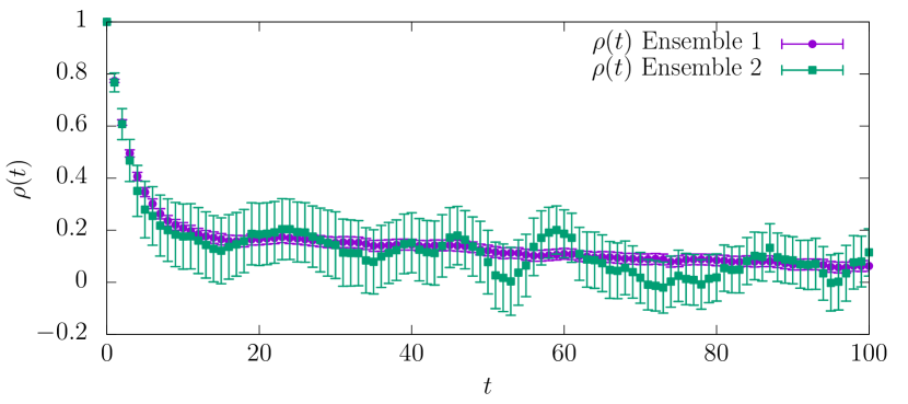
Figure 6: Two replica of a Monte Carlo simulation with $\tau_{\rm exp}=100$. Ensemble 1 has length 20000, while ensemble 2 has length 500. A long Monte Carlo run allows to determine the normalized autocorrelation function $\rho(t)\equiv\Gamma(t)/\sigma^{2}$ more precisely (see Eq. (117)). This results in a more solid estimate of the statistical uncertainties.

Let us end this section commenting that the most common analysis techniques in lattice QCD involves binning the data: the Monte Carlo measurements are averaged in groups of size $N_{\rm bin}$. The data bins are treated as independent measurements and a naive error estimate is performed (usually by resampling). This alternative analysis method does not improve the determinations of the statistical uncertainties over the methods that directly determine the autocorrelation function. It is clear that bins of data are less correlated than the data itself, but it has been shown that the decrease in the correlations is slow $\sim 1/N_{\rm bin}$ [91]. Moreover, in the fairly common case that $N_{\rm bin}$ cannot be taken much larger than the exponential autocorrelation time $\tau_{\rm exp}$, there are no known methods to explicitly include the slow modes of the Markov operator in the binning analysis. On the other hand a direct analysis of the autocorrelation function allows to include these effects in the error estimates [92, 88] (see also the summary in [93]).

In summary, it is important to point out that in contrast with other numerical fields where the number of MC samples is very large, lattice QCD simulations are performed in the uncomfortable situation that the number of samples is not much larger than the relaxation time of the Markov operator. In this situation the estimates of statistical uncertainties can be challenging. This observation is especially relevant for the determinations of the strong coupling, since $\tau_{\rm exp}$ scales like $1/a^{2}$, and fine lattice spacing are needed in order to study observables at short distances.

5 Decoupling of heavy quark and matching accross thresholds

5.1 Decoupling Theorem

Following a Wilsonian approach to field theory, it is natural to imagine that the low-energy dynamics is not sensitive to the details of the theory at high energies – the high-energy degrees of freedom are integrated out. More precisely, when considering observables defined at some low-energy scale $\mu$, the effects of heavy states of mass $m$ are expected to be encoded in a redefinition of the couplings, or suppressed by powers of $\mu/m$ in the limit where $\mu/m\ll 1$.

The original idea of decoupling of massive states dates back to the seminal paper by Appelquist & Carazzone [94], where decoupling was proven by analysing the behaviour of Feynman diagrams containing heavy quark loops in perturbation theory. In order to be able to discuss decoupling, the relevant quantities need to be precisely defined. It is therefore useful to summarise, briefly, the results in Ref. [94], paying specific attention to the subtleties due to the regularization and renormalization of the theory. Since we are ultimately interested in QCD, we can follow the arguments in [94] starting from a non-Abelian gauge theory coupled to a massive fermion as defined in Eq. 1. Working in the Landau gauge, we choose an on-shell renormalization scheme, and denote the renormalized mass and coupling constant $\bar{m}_{\mathrm{os}}$ and $\bar{g}_{\mathrm{os}}$ respectively. The gluon propagator, the three-gluon vertex and the fermion propagator are given respectively by

$$D_{\mu\nu}^{ab}(k)=\delta^{ab}\,\frac{1}{k^{2}}\left(g_{\mu\nu}-\frac{k_{\mu}k_{\nu}}{k^{2}}\right)\,d\left(\frac{k^{2}}{\mu^{2}},\frac{\bar{m}_{\mathrm{os}}^{2}}{\mu^{2}},\bar{g}_{\mathrm{os}}(\mu)\right)\,,$$ (121)

$$i\Gamma^{abc}_{\mu\nu\sigma}(p,q,r)=f^{abc}\,\left[\left(p-q\right)_{\mu}g_{\nu\sigma}+\left(q-r\right)_{\nu}g_{\sigma\mu}+\left(r-p\right)_{\sigma}g_{\mu\nu}\right]\times$$

$$\quad\times G\left(\frac{k^{2}}{\mu^{2}},\frac{\bar{m}_{\mathrm{os}}^{2}}{\mu^{2}},\bar{g}_{\mathrm{os}}(\mu)\right)\,,$$ (122)

$$S(p)=\frac{1}{p^{2}-m^{2}}\left[a\left(\frac{p^{2}}{\mu^{2}},\frac{\bar{m}_{\mathrm{os}}^{2}}{\mu^{2}},\bar{g}_{\mathrm{os}}(\mu)\right)\not{p}+b\left(\frac{p^{2}}{\mu^{2}},\frac{\bar{m}_{\mathrm{os}}^{2}}{\mu^{2}},\bar{g}_{\mathrm{os}}(\mu)\right)m\right]\,,$$ (123)

where in Eq. 5.1, the 1PI vertex is evaluated at a symmetric point $p^{2}=q^{2}=r^{2}=k^{2}$. The mass counterterm is adjusted by imposing that the fermion propagator has a pole for $p^{2}=\bar{m}_{\mathrm{os}}^{2}$, and the remaining counterterms are defined by providing renormalization conditions at the scale $\mu$, e.g.

$$d\left(-1,\frac{\bar{m}_{\mathrm{os}}^{2}}{\mu^{2}},\bar{g}_{\mathrm{os}}(\mu)\right)=1\,,$$ (124)

$$G\left(-1,\frac{\bar{m}_{\mathrm{os}}^{2}}{\mu^{2}},\bar{g}_{\mathrm{os}}(\mu)\right)=1\,,$$ (125)

$$a\left(-1,\frac{\bar{m}_{\mathrm{os}}^{2}}{\mu^{2}},\bar{g}_{\mathrm{os}}(\mu)\right)=1\,.$$ (126)

The running coupling constant at a generic scale $k^{2}$ is defined as

$$\bar{g}_{\mathrm{os}}\left(\frac{k^{2}}{\mu^{2}},\frac{m^{2}}{\mu^{2}},\bar{g}_{\mathrm{os}}(\mu)\right)=\bar{g}_{\mathrm{os}}(\mu)\,G\left(\frac{k^{2}}{\mu^{2}},\frac{m^{2}}{\mu^{2}},\bar{g}_{\mathrm{os}}(\mu)\right)\,d\left(\frac{k^{2}}{\mu^{2}},\frac{m^{2}}{\mu^{2}},\bar{g}_{\mathrm{os}}(\mu)\right)^{3/2}\,,$$ (127)

and its dependence on the scale is described by the beta function:

$$k^{2}\frac{d}{dk^{2}}\bar{g}_{\mathrm{os}}=\beta\left(\frac{\bar{m}_{\mathrm{os}}^{2}}{-k^{2}},\bar{g}_{\mathrm{os}}\right)\,.$$ (128)

The specific value of the coupling at the scale $\mu$ that was used in the renormalization process serves as the initial condition for integrating the beta function. Note that, as pointed out in the original derivation in Ref. [94], the beta function depends on the renormalized mass $\bar{m}_{\mathrm{os}}$ through the ratio $\bar{m}_{\mathrm{os}}^{2}/k^{2}$ – this is a direct consequence of working in an on-shell scheme, where the mass of the particle enters explicitly in the renormalization conditions and therefore in the running of the coupling constant.

In this specific scheme, Appelquist & Carazzone show that diagrams containing heavy propagators are suppressed by powers of $k/\bar{m}_{\mathrm{os}}$ or $\mu/\bar{m}_{\mathrm{os}}$, where $k$ is the typical scale of the external momenta of the diagram. The second, important, result is that, in the decoupling limit, the beta function of the theory in Eq. 128 reduces to the beta function of the theory where the heavy particle has been integrated out, i.e. in this particular case the beta function of pure Yang-Mills theory; the effects of the heavy states simply show up as power corrections that interpolate between the two theories.

5.2 Matching Theories

It was noted in Refs. [95, 96] that the decoupling theorem does not apply in minimal subtraction (MS), since all loops contribute to the beta function independently of the mass of the state. The same problem exists for generic mass-independent schemes [97]. The solution to this problem is found by matching at low energies the theory with heavy particles to an effective theory containing only the light degrees of freedom, i.e. by tuning the couplings of the effective theory so that it reproduces the field correlators of the full theory at low energies up to corrections that are suppressed by the ratio of the scales that characterise the light and heavy degrees of freedom respectively. Matching gauge theories across thresholds is first discussed in Ref. [18], then analysed in detail in Refs. [98, 19]. It has become the method of choice to define the coupling constant at energies that span a wide range and hence cross several mass thresholds.

Once again we find it useful to give a pedagogical review of the main steps in the procedure. We consider a theory with $n_{f}$ light fermions and only 1 heavy fermion , whose dynamics is specified by a lagrangian $\mathcal{L}$ and a set of bare couplings and fields:

$$g,m,m_{h},\xi,\psi,A_{\mu},c\,.$$ (129)

Using a familiar notation for QCD, $g$ is the gauge coupling, $m$ the mass of the light fermions, $m_{h}$ the mass of the heavy fermion, and $\xi$ is the gauge parameter. The fields $\psi,A_{\mu},c$ describe the fermions, the gauge field and the ghosts respectively.

The effective low-energy theory will be a theory defined by an effective lagrangian $\mathcal{L}^{\prime}$ which only involves the light degrees of freedom, and a set of rescaled couplings and fields. Following Ref. [99], the bare couplings and fields of the effective theory are denoted by primed letters, and are connected to the bare couplings and fields of the full theory through the so-called decoupling constants $\zeta_{i}$:

$$g^{\prime}=\zeta_{g}g\,,\quad m^{\prime}=\zeta_{m}m\,,\quad\xi^{\prime}-1=\zeta_{3}\left(\xi-1\right)\,,$$ (130)

$$\psi^{\prime}=\sqrt{\zeta_{2}}\psi\,,\quad A^{\prime}_{\mu}=\sqrt{\zeta_{3}}A_{\mu}\,\quad c^{\prime}=\sqrt{\tilde{\zeta}_{3}}c\,.$$ (131)

It is easy to argue on symmetry grounds that $\mathcal{L}^{\prime}$ must have the same form as $\mathcal{L}$, but contain only the light degrees of freedom:

$$\mathcal{L}^{\prime}\left(g,m,\xi,\psi,A_{\mu},c;\zeta_{i}\right)=\mathcal{L}\left(g^{\prime},m^{\prime},\xi^{\prime},A^{\prime}_{\mu},c^{\prime}\right)\,.$$ (132)

Higher-dimensional operators can appear in $\mathcal{L}^{\prime}$, but are suppressed by inverse powers of the heavy mass. The decoupling constants $\zeta_{i}$ are determined by computing field correlators in both theories, and matching them up to power contributions.

The matching procedure yields the relation between the renormalised coupling $\bar{\alpha}$ in the two theories:

$$\bar{\alpha}^{\prime}(\mu)=\left(\frac{Z_{g}}{Z^{\prime}_{g}}\zeta_{g}\right)^{2}\bar{\alpha}(\mu)=\zeta_{Rg}^{2}\bar{\alpha}(\mu)\,,$$ (133)

where $Z_{g}$ and $Z^{\prime}_{g}$ are respectively the renormalization constants for the coupling in the full and in the effective theory. The decoupling constant $\bar{\zeta}_{g}$ has a perturbative expansion

$$\bar{\zeta}_{Rg}=1+\sum_{\ell=1}^{\infty}\bar{\alpha}(\mu)^{\ell}C_{\ell}(x)\,,$$ (134)

where the coefficients $C_{\ell}$ are functions of the logarithm of the ratio of scales $x=\log\left(\mu^{2}/\bar{m}_{h}(\mu)^{2}\right)$, and $\bar{m}_{h}(\mu)$ is the mass of the heavy fermion in $\overline{\rm MS}$.

It is interesting to recall here that the functional dependence of the coefficients $C_{\ell}$ on $x$ is dictated by the renormalization group equations, as discussed eg. in Ref. [19]. Keeping in mind that

$$\mu^{2}\frac{d}{d\mu^{2}}x=1+\gamma=1+\sum_{k=1}^{\infty}\gamma_{k}\bar{\alpha}(\mu)^{k}\,,$$ (135)

where $\gamma$ is the mass anomalous dimension, we can take the derivative of Eq. 133 with respect to the logarithm of $\mu^{2}$, and solve the resulting equation order by order in $\bar{\alpha}(\mu)$. This procedure yields a set of differential equations that the functions $C_{\ell}$ must satisfy, viz.

$$\frac{d}{dx}C_{1}(x)=\beta_{0}^{\prime}-\beta_{0}\,,$$ (136)

$$\frac{d}{dx}C_{2}(x)=2\left(\beta_{0}^{\prime}-\beta_{0}\right)C_{1}+\beta_{1}^{\prime}-\beta_{1}-\gamma_{0}\frac{d}{dx}C_{1}\,,$$ (137)

$$\dots$$ (138)

The structure of these equations implies that $C_{\ell}$ is a polynomial of degree $\ell$. The coefficients of these polynomials are functions of the coefficients $\beta_{k}$, $\beta_{k}^{\prime}$ and $\gamma_{k}$. On top of that, for each differential equation, an integration constant $C_{\ell,0}$ appears, which is determined by matching a vertex function at $\ell$ loops. The simplest example is the integration of Eq. 136, which yields

$$C_{1}(x)=\left(\beta_{0}^{\prime}-\beta_{0}\right)x+C_{1,0}\,.$$ (139)

As discussed above, $C_{1}$ is a linear function of $x$, the slope of the function is given by the difference of the first coefficients of the beta functions in the two theories, $\beta_{0}$ and $\beta_{0}^{\prime}$, while the integration constant $C_{1,0}$ needs to be computed from a one-loop matching. Recent matching calculations up to four loops are available [21, 17].

The final result for the matching of couplings across mass thresholds is reported in the PDG [100]; using the PDG notation and for the particular case $\mu=m_{\rm h}^{\star}$, we have

$$\alpha_{s}^{(n_{f}+1)}(\mu^{2})=\alpha_{s}^{(n_{f})}(\mu^{2})\left(1+\sum_{\ell=2}^{\infty}c_{\ell}\left[\alpha_{s}^{(n_{f})}(\mu^{2})\right]^{\ell}\right)\,,$$ (140)

here $\alpha_{s}^{(n_{f})}$ is the coupling in the $\overline{\rm MS}$ scheme with $n_{f}$ massless fermions, and $m_{\rm h}^{\star}$ is the mass of the heavy fermion, also defined in the $\overline{\rm MS}$ scheme, at the energy scale given by the mass itself. Note that for this particular choice of scales the $\mathcal{O}(\alpha^{2})$ term in the relation between couplings vanish. The coefficients $c_{n}$ for $n\leq 4$ and the physically relevant cases $3\to 4$ and $4\to 5$ are available in table 2. We also quote the effect that the last term of the series $c_{4}\left[\alpha_{s}^{(n_{f})}(\mu^{2})\right]^{4}$ has in the determination of the strong coupling. As the reader can see, the truncation of the perturbative series in the decoupling relations has a completely negligible effect on the extraction of $\alpha_{s}$ ($\lesssim 0.2\%$ for the case of the charm quark). Note that this analysis does not exclude potentially large non-perturbative corrections in the matching between theories (see next section).

	$m_{\rm h}$ [GeV]	$c_{2}\times 10^{2}$	$c_{3}\times 10^{2}$	$c_{4}\times 10^{2}$	$\delta\alpha_{\overline{\rm MS}}(M_{Z})$ [%]
$3\to 4$	$m_{\rm c}\approx 1.3$	-1.547963	-2.315990	-1.922535	0.18%
$4\to 5$	$m_{\rm b}\approx 4.2$	-1.547963	-2.042976	-0.7278004	0.02%

Table 2: Coefficients for the decoupling of the charm quark ($3\to 4$) and the bottom quark ($4\to 5$) for the case $\mu=m_{\rm h}$ (see Eq. (140)) [17, 21, 101]. The last column quotes the effect of the last known term in the series in the value of the strong coupling at the scale $M_{Z}$.

5.3 Nonperturbative decoupling

As noted before in Sect. 2.1, the running of the coupling constant with the energy scale is determined by the knowledge of the beta function and the $\Lambda$-parameter of a given theory. Hence the matching of the coupling between theories described in the sections above can be reformulated in terms of the matching of the $\Lambda$-parameters, which leads naturally to a framework where decoupling can be discussed beyond perturbation theory. We present here a brief summary of the ideas that were originally developed in Ref. [102].

Following the notation introduced above, we denote quantities in the theory with heavy particles with unprimed variables, while primed variables always refer to the effective theory that includes the light degrees of freedom only. The relation between the $\Lambda$-parameters is fixed by requiring that low-energy quantities are matched up to power corrections; without loss of generality we can write

$$\Lambda^{\prime}=f\left(\Lambda,M\right)\,,$$ (141)

where $M$ is the RGI mass of the heavy particle in the full theory. Furthermore, we can argue on dimensional grounds that

$$\Lambda^{\prime}/\Lambda=P\left(M/\Lambda\right)\,.$$ (142)

The dependence of $P$ on the mass $M$ is encoded in

$$\eta(M)=\left.\frac{1}{P}M\frac{\partial}{\partial M}P\right|_{\Lambda}\,,$$ (143)

which can be reliably evaluated in perturbation theory only for large values of $M$

$$\eta(M)\raisebox{-0.43057pt}{ $\stackrel{{\scriptstyle\small{M\to\infty}}}{{\sim}}$}\eta_{0}+\eta_{1}\bar{g}^{2}(M)+\ldots\,.$$ (144)

Introducing the variable $\tau=\log\left(M/\Lambda\right)$, and integrating Eq. 144, yields

$$P\left(M/\Lambda\right)=\frac{1}{k}\,\exp\left(\eta_{0}\tau\right)\,\tau^{\eta_{1}/(2b_{0})}\times\left(1+O\left(\frac{\log\tau}{\tau}\right)\right)\,,$$ (145)

where $k$ is a constant that can be computed given the conventions for $\Lambda$ and $M$.

A nonperturbative matching condition requires that some hadronic scale remains the same in the two theories, ie.

$$m_{\mathrm{had}}^{\prime}\left(\Lambda^{\prime}\right)=m_{\mathrm{had}}\left(\Lambda,M\right)+O\left(\frac{\Lambda^{2}}{M^{2}}\right)\,.$$ (146)

In the equation above $\Lambda$ and $M$ are dimensionful quantities that define the coupling and the masses in the full theory, and are given. The matching condition then determines $\Lambda^{\prime}$. As a consequence we find:

$$\frac{m_{\mathrm{had}}\left(\Lambda,M\right)}{\Lambda}=\frac{m_{\mathrm{had}}^{\prime}\left(\Lambda^{\prime}\right)}{\Lambda^{\prime}}\frac{\Lambda^{\prime}}{\Lambda}+O\left(\frac{\Lambda^{2}}{M^{2}}\right)\,,$$ (147)

and hence

$$\frac{m_{\mathrm{had}}\left(\Lambda,M\right)}{m_{\mathrm{had}}\left(\Lambda,0\right)}=Q_{\mathrm{had}}\,P\left(M/\Lambda\right)+O\left(\frac{\Lambda^{2}}{M^{2}}\right)\,,$$ (148)

where

$$Q_{\mathrm{had}}=\frac{m_{\mathrm{had}}^{\prime}\left(\Lambda^{\prime}\right)}{\Lambda^{\prime}}\frac{\Lambda}{m_{\mathrm{had}}\left(\Lambda,0\right)}\,.$$ (149)

The left-hand side of Eq. 148 can be measured by performing MC simulations of the full theory with different values of the mass $M$, while $Q_{\mathrm{had}}$ requires an extra simulation in the effective theory.

References [102, 22] study the effect of heavy quarks along the lines described above. Making a long story short, they estimate the non-perturbative effects in the matching between theories with the conclusions that for the most important case of the charm quark, they affect the extraction of $\alpha_{s}$ below the $0.4\%$ level. The interested reader is invited to consult the original works.

6 Convenient observables for a coupling definition

In principle there are very many possibilities to define the strong coupling on the lattice. The only thing that is needed is a dimensionless finite observable that depends on a single scale. Our discussion on scale setting (in particular the discussion about theory scales in section 4.5.3) has already introduced some observables with these characteristics. In this section we will introduce the observables that are more commonly used to compute the strong coupling from the lattice, with special emphasis on the systematic effects associated with the truncation of the perturbative series.

We recall that the general method to extract the value of the strong coupling consists in comparing a perturbative theoretical prediction with lattice measurements (i.e. eq. (36)). It is convenient to introduce non-perturbative definitions of the coupling constant, where the value of the observable is used for the definition of the strong coupling. We take a dimensionless observable with perturbative expansion

$$O(\mu)\raisebox{-0.43057pt}{ $\stackrel{{\scriptstyle\small{\alpha_{\overline{\rm MS}}\to 0}}}{{\sim}}$}\sum_{k=1}c_{k}(\mu/\mu^{\prime})\alpha_{\overline{\rm MS}}(\mu^{\prime})\,,$$ (150)

and define

$$\alpha_{O}(\mu)=\frac{O(\mu)}{c_{1}(1)}\,.$$ (151)

This equation defines a particular renormalization scheme, which we refer to as $O$-scheme. When computed on the lattice, $O(\mu)$ can be determined at all energy scales, thus providing a non-perturbative renormalization scheme.

Note that the RG equation for the coupling in the $O$-scheme defines a $\beta$-function, that can also be computed beyond perturbation theory

$$\mu\frac{{\rm d}\bar{g}_{O}(\mu)}{{\rm d}\mu}=\beta_{O}(\bar{g}_{O})\raisebox{-0.43057pt}{ $\stackrel{{\scriptstyle\small{g_{O}\to 0}}}{{\sim}}$}-g_{O}^{3}(b_{0}+b_{1}g_{O}^{2})+\dots\,.$$ (152)

This $\beta$-function has all the properties that one would expect, starting from a perturbative expansion with the usual first two universal terms. Examining the convergence of the perturbative series of this beta function provides a piece of information on the size of the truncation effects in the determination of the strong coupling. If these are small, the beta function $\beta_{O}(x)$ has to be well approximated by its perturbative expansion. Note also that our fundamental relation Eq. 16 allows the determination of the $\Lambda$-parameter in this scheme ($\Lambda_{O}$). Figure 7 shows the $\beta$-function for the typical choices of observables that we are going to explore in detail later.

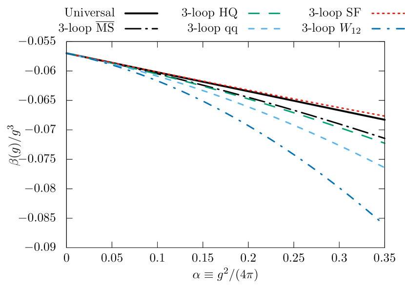
Figure 7: $\beta$-function in three flavor QCD in different schemes (see Eq. 152). The 2-loop universal behavior is compared with the 3-loop $\beta$-function in different schemes: $\alpha_{\rm HQ,4}$ (Eq. (171)), $\alpha_{\rm qq}$ (Eq. (163)), $\alpha_{\rm SF}$ (Eq. (196)) and $\alpha_{W_{12}}$ (Eq. (175)). With the exception of the scheme based on Wilson loops, where the 3-loop coefficient is significantly larger than in the $\overline{\rm MS}$ scheme, all schemes seem well behaved from a perturbative point of view. Note that for the case of the static potential, one more order is known perturbatively.

Observable	$l$	$\alpha_{\overline{\rm MS}}(\mu_{\rm PT})$	$\mu_{\rm PT}$ [GeV]	Power corrections
QCD vertices	3	$0.20-0.30$	$2-6$	${\sim 1/\mu^{2},1/\mu^{6}}^{+}$
Static Potential	3	$0.19-0.36^{\star}$	$1.5-8^{\star}$	-⋆
HQ correlators	2	$0.20-0.36^{\dagger}$	$\bar{m}_{c}^{\dagger}-4\bar{m}_{c}^{\dagger}$	-
Wilson loops	2	$0.22-0.40$	$1/a=1.1-4.4$	${\sim 1/\mu^{2}}^{\ddagger}$
Vacuum polarization	4	$0.22-0.31$	$1.6-4$	$\sim 1/p^{2k}\,(k=1,...,4)$
Finite size scaling	2	$0.11-0.23$	$4-140$	-

Table 3: We summarize some key numbers in different techniqes used to determine the strong coupling. Column labeled $l$ gives the number of loops known in the perturbative expansion of the $\beta$-function. The second and third columns shows the range of couplings that have been explored in the literature, and the corresponding energy scale (note however that not all individual works explore the same energy scales). Finally we show if power corrections are needed to describe the data, and how many terms are used.
⁺ Most of the determinations find it neccesary to add these power corrections in order to describe the lattice data. Nevertheless, see [103, 104].
^⋆ Most of the works expore this range of scales without any need for power corrections. In [105] power corrections are added to the analysis, allowing to use data down to 0.6 GeV.
^† Most determinations are performed at the charm mass, but some works [106, 107] explore larger masses. See section 6.3 for more details.
^‡ In this approach cutoff effects manifest as power corrections. See 6.4 for more details.

We have explained in detail (see sections 2.2.3, 3.2) the particular systematic effects that affect the lattice determinations of the strong coupling. Let us now focus on explaining how the different methods to extract the strong coupling face these challenges. In particular we will pay special attention to the following issues.

Perturbative truncation effects:

We already insisted on the fact that the determination of the strong coupling has to be understood as an extrapolation (cfr. section 2.2.3 and 3). An important criterion is the range of scales $\mu_{\rm PT}$ at which one matches with perturbation theory. More precisely, we are interested in the values of the coupling $\alpha_{\overline{\rm MS}}^{(l-1)}(\mu_{\rm PT})$ at such scales, where $l$ is the number of analytically known loops in the asymptotic expansion of the $\beta$ function, since they parametrize the leading perturbative truncation effects.

Non perturbative effects:

Power corrections are understood to arise from the Operator Product Expansion (OPE). The short distance observable used to extract the strong coupling $O(\mu)$, typically has an OPE that schematically can be written as

$$O(\mu)=\sum_{k=0}d_{k}(\mu)\frac{O^{(k)}}{\mu^{k}}\,,$$ (153)

where $O^{(k)}$ are operators of dimension $k$. Note that the perturbative expansion of the observable Eq. (151) neglects all power corrections (terms with $k>0$). One problem with these non-perturbative corrections in lattice determinations of the strong coupling is that they are not computed, but estimated from the same data for $O(\mu)$ by fitting them. Distinguishing the perturbative running from the non-perturbative corrections given the limited range of scales that are available in many extractions is always challenging.

Ideally one would like to work with observables and energy scales where the power corrections are negligible. In practice this is not always the case.

6.1 The ghost-ghost-gluon vertex

The definition of the strong coupling using QCD vertices is the one that is more similar to the type of computation that is usually done in the context of perturbation theory. There are several issues in the extraction of these QCD vertices from lattice QCD simulations. In practice the coupling is extracted from the gluon/ghost two-point functions, but these are not gauge invariant, and therefore this scheme can only be implemented by fixing the gauge of the lattice configurations. The problems of gauge fixing beyond perturbation theory (i.e. Gribov ambiguities [108]), have been discussed at length in the literature (see for example [109]), and we can add very little to the discussion, except pointing out that the issue of Gribov ambiguities is also present in other lattice QCD calculations. One of the most widely used methods of non-perturbative renormalization (i.e. “RI/MOM” schemes, see [110]) also requires to fix the configurations (typically the Landau gauge is used). It is believed that at the relatively high energy scales where $\alpha_{s}$ is extracted, this is not a serious issue.

In principle there are several options to extract the strong coupling, since it can be defined from different three- and four-point functions. All the methods define the coupling by requiring that some vertex is equal to its tree-level value. The momenta entering in the vertex are part of the definition of the scheme. The most popular choices set one of the momenta to zero, and are usually labeled $\widetilde{\rm MOM}$ schemes.

Nowadays the most common coupling definition uses the un-renormalized ghost-ghost-gluon vertex, which can be constructed from the gluon and ghost two-point functions. The non-perturbative coupling definition reads

$$\alpha_{T}(\mu)=\lim_{a\to 0}F_{\rm lat}(p,a)D_{\rm lat}(p,a)\frac{g_{0}^{2}}{4\pi}\Big{|}_{\mu=p}\,.$$ (154)

This is usually referred to as the Taylor scheme, as indicated by the suffix. Here $D_{\rm latt}(p,a)$ and $F_{\rm latt}(p,a)$ are the “dressing functions” of the lattice gluon and ghost two-point functions  and $g_{0}^{2}$ is the bare coupling used for the simulation. The main advantage of this scheme is that one does not need to determine any three- or four-point function, since the coupling is directly defined from the computation of the propagators. We are going to focus the discussion on this particular choice, although most of what we are going to state is also valid for other, similarly defined schemes. The perturbative expansion for $\alpha_{T}(\mu)$,

$$\alpha_{T}(\mu)\raisebox{-0.43057pt}{ $\stackrel{{\scriptstyle\small{\mu\to\infty}}}{{\sim}}$}\alpha_{\overline{\rm MS}}(\mu)+t_{1}\alpha_{\overline{\rm MS}}^{2}(\mu)+t_{2}\alpha_{\overline{\rm MS}}^{3}(\mu)+t_{3}\alpha_{\overline{\rm MS}}^{4}(\mu)+\mathcal{O}(\alpha_{\overline{\rm MS}}^{5})\,,$$ (157)

is known up to three-loops [111].

There are two important issues that affect generally these extractions and that are worth mentioning.

Non perturbative corrections

Several studies have concluded that including non perturbative corrections in the analysis is mandatory to find consistent results among observables and range of scales used to determine the $\Lambda$-parameter (see reference [112] for a detailed study in pure gauge and energy scales in the range $3-5$ GeV).

The leading correction comes from

$$\sim\frac{g_{0}^{2}\langle A^{2}\rangle}{p^{2}}\,.$$ (158)

These corrections are included in the analysis either by using an estimate for $\langle A^{2}\rangle$ (like for example [113]) or by fitting their data including such a term. Higher order non-perturbative corrections (i.e. $\sim p^{-x}$ for different values of $x$) are also typically needed to match the lattice data with the perturbative running [114, 115, 116, 113] (see Fig. 8).

Cutoff effects

The range of scales where $\alpha_{T}(\mu)$ can be described by its perturbative expansion (and the non-perturbative contributions) is typically about $\mu\sim 3$ GeV. Since the typical lattice spacings in state-of-the-art lattice simulations are in the range $2-5$ GeV, it is really challenging to make a continuum extrapolation with several lattice spacings in order to extract the value of the coupling at some scale $\mu$. Therefore the common approach is to include several terms to either subtract or fit the cutoff effects (see [114, 115, 116, 117]).

Figure 8 shows these two points exemplified in the results of one particular work [116]. Panel (a) shows that the raw measurements for the Taylor coupling at two different values of the lattice spacing differ by approximately $50\%$ after subtracting the $H(4)$ breaking cutoff effects (see [116] for details). The remaining scaling violations have an asymptotic expansion that includes terms $\sim\mathcal{O}(a^{2}p^{2})$ and are noticeable compared with the statistical precision of the data. Panel (b) shows the extraction of the $\Lambda$-parameter after matching with its perturbative expansion at the scale $\mu$ [113]. The plot shows the values of $\Lambda_{\overline{\rm MS}}$ as a function of $\alpha_{\overline{\rm MS}}^{3}$ (the leading correction to the extraction). The data with only $1/\mu^{2}$ corrections subtracted shows a correction compatible with a large $\alpha^{3}$ perturbative term. But if another non-perturbative term $1/\mu^{6}$ is included as a fit parameter, the data seem to be well described by the perturbative expression in Eq. (157).

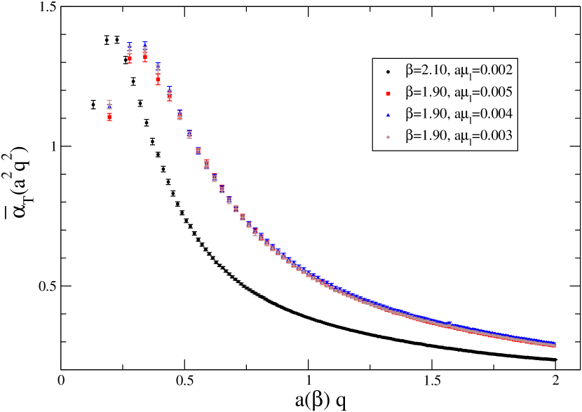
(a)

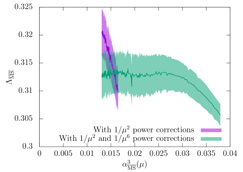
(b)

Figure 8: Extraction of the strong coupling from QCD vertices. (a) Determination of the strong coupling in the Taylor scheme. The figure shows the raw values of the coupling for two different lattice spacing ($a\approx 0.089$ fm for $\beta=1.90$ and $a\approx 0.06$ fm for $\beta=2.10$) and different values of the quark masses. As the reader can see, the chiral dependence is mild, but the cutoff effects are substantial. (source [116]). (b) Extraction of the $\Lambda$-parameter in the Taylor scheme. Including only $1/\mu^{2}$ power corrections is not enough to to reach the perturbative running. In this particular work [113] , the extraction of $\Lambda$ seems consistent in the region $0.012<\alpha^{3}<0.025$ by fitting the data with an additional $1/\mu^{6}$ power correction term.

In summary, the extraction of $\alpha_{s}$ from QCD vertices is hampered by a slow rate of convergence to the perturbative behavior. Several non-perturbative corrections need to be fitted at the same time, since they are noticeable. Even after fitting for the non-perturbative corrections the range of energies that can be used to determine the strong coupling is limited. Large energies scales are needed, where most data come typically from a single lattice spacing.

These extractions also show that distinguishing the perturbative and non-perturbative corrections is, in practice, very difficult. Figure 8 (b) shows the difficulty in distinguishing a correction of order $\alpha^{3}(\mu)$ from a $1/\mu^{6}$ non perturbative correction when we have only access to a limited range of scales. Indeed we see that a variation of the order of 10 MeV in $\Lambda$ can be reabsorbed by higher-order power corrections.

We believe that a dedicated study in pure gauge theory with the aim of reaching energy scales where the non-perturbative data is described by the perturbative prediction without fitting any non-perturbative terms would be very interesting. A pure gauge simulation would also allow a detailed investigation of the continuum extrapolations using several fine lattice spacing.

6.2 The static potential

The force between static color charges has been traditionally one of the first observables to be studied in lattice QCD [118]. The potential at distance $r$ can be extracted from Wilson loops, that behave asymptotically as

$$\mathcal{W}_{r\times T}\sim\lambda_{0}^{2}e^{-V(r)T}+\sum_{k}\lambda_{k}^{2}e^{-V_{n}(r)T}\,.$$ (159)

The potential $V(r)$, given by the ground state (i.e. the leading decaying exponential), is formally computed as

$$V(r)=\lim_{T\to\infty}\frac{1}{T}\log\langle\mathcal{W}_{r\times T}\rangle\,.$$ (160)

In practice it is extracted at large, but finite, values of $T$, and therefore several techniques are needed in order to enhance the overlap with the ground state and to distinguish the leading exponential from the excited state contamination. When computed on the lattice, the static potential is power divergent $\sim 1/a$. This is related to the ambiguity in the overall magnitude of $V(r)$: only energy differences are physical. The cleanest way to deal with this linear divergence is to define the coupling via the static force

$$F(r)=\frac{{\rm d}V(r)}{{\rm d}r}\,.$$ (161)

The derivative with respect to $r$ removes the linear divergence but requires to perform a numerical derivative of the potential. This is implemented by some finite difference expression. It is convenient to define the force by

$$F(r_{I})=\frac{V(r)-V(r-a)}{a}\,,$$ (162)

with $r_{I}$ chosen so that the force has no cutoff effects to leading order in perturbation theory. This has been shown to reduce the cutoff effects in the force [119].

A renormalized coupling constant can be defined non-perturbatively using the static force. The non-perturbative definition of the coupling and its perturbative expansion in powers of the coupling in the $\overline{\rm MS}$-scheme reads

$$\alpha_{qq}(\mu)=\frac{4}{3}r^{2}F(r)\Big{|}_{\mu=1/r} \stackrel{{\scriptstyle\small{r\to 0}}}{{\sim}} \,\alpha_{\overline{\rm MS}}(\nu)+c_{qq}^{(1)}(s)\alpha_{\overline{\rm MS}}^{2}(\nu)+c_{qq}^{(2)}(s)\alpha_{\overline{\rm MS}}^{3}(\nu)$$ (163)

$$+ c_{qq}^{(3)}(s)\alpha_{\overline{\rm MS}}^{4}(\nu)+\dots\qquad(s=\mu/\nu)\,.$$

The relation of this coupling to the $\overline{\rm MS}$ scheme is known up to three loops, but the observable suffers from IR divergences, that manifest themselves in the naive perturbative expansion of eq. (163) being divergent. These so-called soft and ultra-soft divergences can be re-summed and produce logarithmic corrections to the perturbative series. The leading one is $\propto\alpha_{\overline{\rm MS}}^{4}(\nu)\log\alpha_{\overline{\rm MS}}(\nu_{\rm us})$. This re-summation process introduces an arbitrary energy scale (so called ultra-soft scale), its natural value being $\nu_{\rm us}=\alpha(\nu)/r$. In principle this means that not only the scale $\nu\approx 1/r$ has to be large, but also $\nu_{\rm us}=\alpha(\nu)/r$ has to be large. The additional factor $\alpha$ is not negligible taking into account that these extractions take place at a few GeV.

All in all, the perturbative expansion, including terms $\alpha^{4},\alpha^{4}\log\alpha,\alpha^{5}\log\alpha,\alpha^{5}\log^{2}\alpha$, is known [120, 121, 122, 123, 124, 125, 126, 127] (see [128] for a summary on the perturbative expressions).

Regarding the perturbative behavior, figure 7 shows that the $\beta$-function in this scheme is well behaved, with a 2-loop coefficient of a similar size as in the $\overline{\rm MS}$ scheme.

Several works extract the value of the strong coupling not from the force, but directly from the potential. In particular they examine the dimensionless quantity $rV(r)$. Basically the same considerations apply for these works: the perturbative expansion in the $\overline{\rm MS}$ scheme is known up to order $\mathcal{O}(\alpha_{\overline{\rm MS}}^{4})$, and the soft and ultra-soft gluons give rise to logarithmic corrections in the perturbative expansion, starting at order $\alpha_{\overline{\rm MS}}^{4}$. The main difference is in the role of the linear divergence in the potential $V(r)\sim 1/a$.

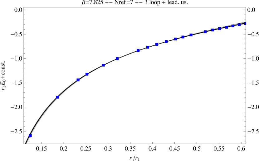
(a)

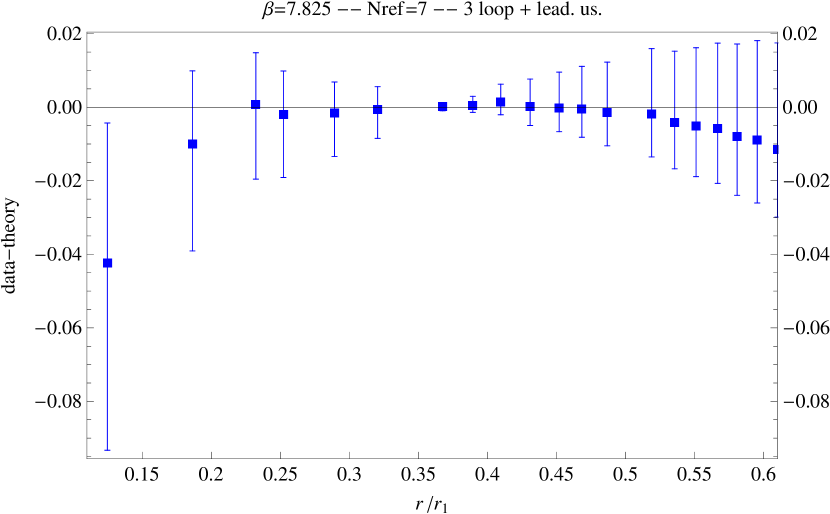
(b)

Figure 9: (a) Comparison of the perturbative prediction and the lattice data at the finest lattice spacings ($a\approx 0.04$ fm) for the static energy $E_{0}(r)$. (b) Residuals of the fit.

Of course there are many different ways to use the perturbative expansion Eq. (163) (or a similar expression for the potential $rV(r)$) to extract $\alpha_{s}$. Different works, although similar in spirit, use different approaches to fit the lattice data and deal with the additive renormalization (in case they use $V(r)$ for the extraction). Here we will focus on one particular work [129] to show the details of such analysis. Ref. [129] uses the expression of the static force and determines the integral up to a reference distance $r_{\rm ref}$,

$$E_{0}(r)=\int_{r_{\rm ref}}^{r}{\rm d}x\,F(x)\,.$$ (164)

The perturbative expansion for the force gives a similar perturbative expansion for $E_{0}(r)$. Note that this quantity is similar to the static potential $V(r)$, with the difference that it is free of the linear divergence $\sim 1/a$ (the relation $E_{0}(r_{\rm ref})=0$ is exact for all lattice spacings), and that depends now on two scales ($r$ and $r_{\rm ref}$). The perturbative expression for $E_{0}(r)$ is fitted to the lattice data. Fig. 9 shows the result of such an analysis. Non-perturbative corrections do not seem to be needed to describe the data at least for distances in the range $r\lesssim 0.2$ fm. This distance is, nevertheless, large enough to allow the analysis with several lattice spacings, so the lattice data can be extrapolated to the continuum. Other recent works include non-perturbative corrections in the analysis of the lattice data either to claim a better convergence [130] or to extend the range described by their fit to $r\lesssim 0.3$ fm [105].

In summary, extracting the strong coupling from the static potential is, in the opinion of the authors, one of the most promising approaches. The N³LO perturbative knowledge, together with the fact that data in this scheme seem to follow the perturbative predictions at scales as low as $1.5$ GeV means that a precise determination can be achieved. In particular, contrary to other approaches, there is no need to fit or parametrize any non-perturbative corrections. At least in theory, the dependence on the lattice spacing, can be accounted for. Conceptually, the fact that the observable used is not IR safe is not ideal. An additional (lower) energy scale enters into the game, and a few works discuss the best methods to deal with these corrections. The main criticism to such extractions, is that their results depends sensibly on the physics at a scale of just a few GeV, in particular the range of scales where their assumptions can be checked (role of the IR divergences, size of cutoff effects, matching with perturbation theory) is limited. It would be interesting to check the agreement with the perturbative running down to higher energies, at least in the pure gauge theory, where very fine lattice spacings can be simulated (see reference [131] for a recent study). We postpone to section 7 a more detailed study.

6.3 Heavy quark correlators

The idea of using correlators of heavy quarks to extract the value of the strong coupling has its origins in a phenomenological determination of $\alpha_{s}$: moments of quarkonium correlators in the vector channel can be compared with experimental data for $e^{+}e^{-}\to\text{hadrons}$.

As was first noted by the HPQCD collaboration [132], the strong coupling and the charm quark mass can be extracted on the lattice from correlators of the pseudoscalar density involving two heavy quarks,

$$G(x_{0})=a^{6}(am_{0})^{2}\sum_{\mathbf{x}}\langle\overline{\psi}\gamma_{5}\psi(\mathbf{x},x_{0})\,\overline{\psi}\gamma_{5}\psi(\mathbf{0},0)\rangle\,,$$ (165)

where $am_{0}$ is the bare quark mass. This correlator has a short distance divergence $\sim 1/x_{0}^{3}$, but if one uses a fermion formulation that preserves some chiral symmetry (like staggered or domain wall fermions), the PCAC relation ensures that moments of $G(x_{0})$, defined as

$$G_{n}=\sum_{x_{0}}\left(\frac{x_{0}}{a}\right)^{n}G(x_{0})\,,$$ (166)

are dimensionless quantities with a well defined continuum limit  for $n\geq 4$. The main contribution to these moments comes from Euclidean times $x_{0}\sim 1/m$.

The extraction of the strong coupling is performed using the reduced even moments

$$r_{4} = \frac{G_{4}}{G_{4}^{(0)}}\,,$$ (167)

$$r_{n} = \bar{m}(\mu)\frac{am_{\eta}}{2am_{0}}\left[\frac{G_{n}}{G_{n}^{(0)}}\right]\,,\qquad(n\geq 6)$$ (168)

where $G_{n}^{(0)}$ denotes the leading order prediction for $G_{n}$ in bare lattice perturbation theory. This normalization is introduced in order to reduce cutoff effects (i.e. to leading order, $r_{n}$ is free of lattice artifacts). Here $m_{\eta}$ denotes the mass of the $\eta_{c}$ meson, and $r_{n}$ admits a perturbative expansion that allows an extraction of the strong coupling constant:

$$r_{n}\raisebox{-0.43057pt}{ $\stackrel{{\scriptstyle\small{\alpha_{\overline{\rm MS}}(\mu)\to 0}}}{{\sim}}$}1+r_{n,1}\alpha_{\overline{\rm MS}}(\mu)+r_{n,2}(s)\alpha_{\overline{\rm MS}}^{2}(\mu)+r_{n,3}(s)\alpha_{\overline{\rm MS}}^{3}(\mu)+\dots$$ (169)

where

$$s=\frac{\mu}{\bar{m}(\mu)}\,.$$ (170)

A non-perturbative definition of the strong coupling at the scale $\bar{m}(\bar{m})$ is given by

$$\alpha_{\rm HQ,n}(\mu)\Big{|}_{\mu=\bar{m}(\bar{m})}=\frac{r_{n}-1}{r_{n,1}}\raisebox{-0.43057pt}{ $\stackrel{{\scriptstyle\small{\alpha_{\overline{\rm MS}}(\mu)\to 0}}}{{\sim}}$}\alpha_{\overline{\rm MS}}(\nu)+\frac{r_{n,2}(s)}{r_{n,1}}\alpha_{\overline{\rm MS}}^{2}(\nu)+\frac{r_{n,3}(s)}{r_{n,1}}\alpha_{\overline{\rm MS}}^{3}(\nu)+\dots\,,$$ (171)

with $s=\nu/\bar{m}(\bar{m})=\nu/\mu$. The first three coefficients ($r_{n,1},r_{n,2}(s),r_{n,3}(s)$) are analytically known (see [133, 134, 135, 136]. Reference [107] has values tabulated for $N_{\rm f}=3$).

There are two crucial points in these determinations: the estimate of the truncation uncertainties, and controlling the continuum extrapolations. Note that these two points have competing interests: the continuum extrapolation is more easily kept under control for a quantity measured at larger distances, and therefore the “high” moments $r_{6,8,10}$ have milder continuum extrapolations. On the other hand the truncation uncertainties are smaller for a short distance quantity: the first moment $r_{4}$ has a better behavior. This is just another manifestation of the “window problem” (see figure 2).

The estimates for these uncertainties vary significantly across different studies, and we will comment in detail on the issue of the truncation uncertainties in section 7. Here we will focus on the more technical issue of the continuum extrapolation. Figure 10 shows the continuum extrapolation of $r_{4}$ at scale $m_{\rm c}$ of the works [137, 106]. As the reader can see, the scaling violations are significant and have a complicated functional form. Different works in the literature deal with these complicated cutoff effects in very different ways

JLQCD collaboration [138]:

In this case they prefer to only perform extrapolations linearly in $a^{2}$. Their data for $r_{4}$ does not allow such an extrapolation, and therefore it is excluded from their analysis.

HPQCD collaboration [107, 139]:

In these works all moments are used, and masses above the charm quark mass are used, including data with $am\sim 0.9$. Cutoff effects are large and the data is contaminated by effects $\sim(am_{\rm c})^{2p}$. Therefore their fit Ansatz includes terms $a^{2p}$ with $p$ up to 10. These fits typically have more terms than data, and require to include an estimate of the size of these coefficients as Bayesian priors.

Ref. [106]:

Here energy scales larger than the physical charm quark mass are explored, but the continuum extrapolations are difficult and the data usually has associated large uncertainties (see figure 10).

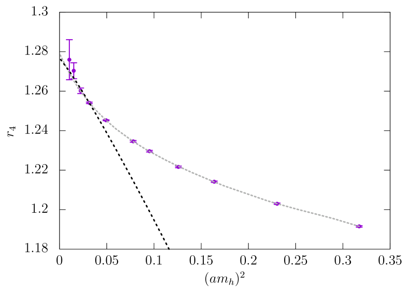
(a)

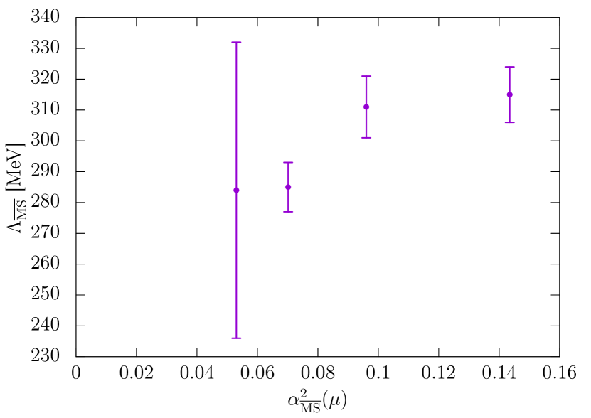
(b)

Figure 10: (a) Continuum extrapolation of $r_{4}$ at the lower energy scale $\mu\sim\bar{m}_{c}$. Scaling violations are significant, even at the smaller quark masses used in the study. The extrapolations is performed using both a 5${}^{\underline{th}}$ degree polynomial, or a second degree one with a restricted fitting window (source [106]). (b) Dependence of the $\Lambda_{\overline{\rm MS}}$ parameter extacted using heavy quark correlators on the value of the coupling at the matching scale with perturbation theory ($\alpha_{\overline{\rm MS}}(\mu)$) (source [106]).

The main drawback of this approach is the large cutoff effects that affect the quantity used to extract the strong coupling. This makes it very challenging to explore energy scales larger than the physical charm quark mass $m_{c}\sim 1.4$ GeV, which is not particularly large. The recent work in Ref. [106] explores different energy scales in the range $\bar{m}_{c}-3\bar{m}_{c}$, but the continuum extrapolation is very challenging already at $\mu\gtrsim 2m_{c}$ . Even at the scale of the charm quark mass, scaling violations are significant and have a complicated functional form (see Figure 10). Together with the fact that the perturbative relation is known only to NNLO the situation is far from ideal: truncation uncertainties at the energy scales reached by current simulations are not small (see detailed discussion in section 7.2.3). This might change in the future, as smaller lattice spacings can be simulated, allowing a reduction of the discretization effects. A detailed study in pure gauge and reaching energy scales significantly larger than the charm quark mass, would probably give very important information on the systematics of this method.

6.4 Observables defined at the scale of the cutoff

Lattice QCD offers the interesting possibility of extracting the strong coupling from expectation values computed at non-zero lattice spacing. This approach is fundamentally different from the strategies outlined above, where a quantity is computed in QCD (i.e. extrapolated to the continuum), and then compared with a perturbative prediction. The observables that we are going to discuss in this subsection are defined at a scale given by the lattice spacing $1/a$. Lattice bare perturbation theory is able to relate these purely lattice observables with a power series in the renormalized coupling. The usual problem that a naive approach has to face is that bare lattice perturbation theory is just terrible. Absurdly small values of the lattice coupling $\alpha_{\rm latt}=g_{0}^{2}/4\pi$ have to be used in order to reach the domain of apparent convergence. It has been argued that this apparent failure of lattice perturbation theory is just a due to the choice of the bare coupling $g_{0}^{2}$ as expansion parameter [140]. If lattice quantities are expressed as a perturbative series in a renormalized coupling, like $\alpha_{\overline{\rm MS}}(\mu)$, their perturbative behavior improves substantially (see [140]).

The HPQCD collaboration has pursued the systematic study of several Wilson loops of size $n\times m$ (denoted $\langle W_{nm}\rangle$) and used them to extract the value of the strong coupling. In these analyses lattice quantities are expressed as a perturbative series in terms of the renormalized coupling $\alpha_{V}(\mu)$; for an SU(3) gauge theory coupled to $N_{f}$ fermions in the fundamental representation, the latter coupling is defined by [123]

$$\alpha_{\rm V}(\mu)=\alpha_{\overline{\rm MS}}(\bar{\mu})+\frac{2.6-0.3N_{\rm f}}{\pi}\alpha_{\overline{\rm MS}}^{2}(\bar{\mu})+\frac{53.4-7.2N_{\rm f}+0.2N_{\rm f}^{2}}{\pi^{2}}\alpha_{\overline{\rm MS}}^{3}(\bar{\mu})\,,$$ (172)

with $\bar{\mu}=\exp(\gamma-5/6)\mu\approx 0.774\times\mu$. Wilson loops have a perturbative expansion

$$-\log\langle W_{nm}\rangle\raisebox{-0.43057pt}{ $\stackrel{{\scriptstyle\small{a\to 0}}}{{\sim}}$}w_{1}\alpha_{\rm V}(\mu)+w_{2}\alpha_{\rm V}^{2}(\mu)+w_{3}\alpha_{\rm V}^{3}(\mu)+\dots\,.$$ (173)

Alternatively one can use Creutz ratios or tadpole improved Wilson loops. This latter choice

$$-\log\left(\frac{\langle W_{nm}\rangle}{\sqrt{\langle W_{11}\rangle^{n+m}}}\right)\raisebox{-0.43057pt}{ $\stackrel{{\scriptstyle\small{a\to 0}}}{{\sim}}$}w_{1}^{\rm b}\alpha_{\rm V}(\mu)+w_{2}^{\rm b}\alpha_{\rm V}^{2}(\mu)+w_{3}^{\rm b}\alpha_{\rm V}^{3}(\mu)+\dots\,.$$ (174)

is supposed to lead to smaller truncation uncertainties. In all cases the perturbative coefficients are known for several choices of $n,m$ [141]. The scale is given by $\mu=d/a$, where $d\approx\pi$ with the exact value depending on the choice of Wilson loop. Note that non-perturbative couplings can be defined by expressions

$$\alpha_{W_{nm}}(1/a)=-\frac{\log\langle W_{nm}\rangle}{w_{1}}\raisebox{-0.43057pt}{ $\stackrel{{\scriptstyle\small{a\to 0}}}{{\sim}}$}\alpha_{\rm V}(\mu)+\frac{w_{2}}{w_{1}}\alpha_{\rm V}^{2}(\mu)+\frac{w_{3}}{w_{1}}\alpha_{\rm V}^{3}(\mu)+\dots\,.$$ (175)

Several quantities are fitted to the previous perturbative expressions, with the value of $\alpha_{\rm V}(\mu_{\rm ref})$ as fit parameter. The values of $\alpha_{\rm V}(\mu)$ at other scales are obtained from $\alpha_{\rm V}(\mu_{\rm ref})$ and the RG equation

$$\mu^{2}\frac{{\rm d}\alpha_{\rm V}(\mu)}{{\rm d}\mu^{2}}=-\alpha_{\rm V}^{2}\sum_{k=0}^{3}\beta_{k}\alpha_{\rm V}^{k}\,.$$ (176)

The final value of $\alpha_{\rm V}(\mu_{\rm ref})$ can be converted to the more convenient $\overline{\rm MS}$ scheme using Eq. (172).

An example of such extractions are the HPQCD works (see [132]). A total of 22 quantities (all like Eq. (173)) are fitted to their perturbative expression. Unfortunately the truncated perturbative expression Eq. (173) does not describe the data well, and several extra terms (up to $\alpha_{{\rm V}}^{10}$) are necessary in order to obtain a sensible fit. The coefficients of these terms are constrained with Gaussian priors, which eventually lead to stable fits, with a consistent determination of the strong coupling using any of the 22 quantities (although some of them require to also fit several power corrections).

The main advantage of methods based on observables defined at the cutoff scale, is that high energies can be reached without having to worry about the continuum extrapolation. The statistical accuracy is excellent, since the observables entering the determination Eq. (173) have a very small variance. On the other hand the uncertainty in these determinations is dominated by the truncation of the perturbative series. The fact that several higher order terms have to be fitted (and constrained with Gaussian priors) in order to describe the data is not ideal. It is clear that expressing lattice quantities as a power series in renormalized couplings, as suggested in [140] greatly improves the predictive power of perturbation theory (bare perturbation theory is just useless). Still these lattice observables are far from ideal from a perturbative point of view: even if energy scales $1/a\approx 4$ GeV are reached, perturbation theory does not predict the lattice data and truncation uncertainties are not small (see detailed discussion in section 7.2.4).

Another delicate point in this approach is that cutoff effects have the same functional form as the non-perturbative effects (power corrections) in the expansion of $\alpha_{P}(1/a)$. This can be easily understood by noting that

$$a^{2}\sim\exp\left\{-\frac{4\pi}{2b_{0}\alpha_{W}(1/a)}\right\}\,,$$ (177)

Of course in any extraction of the strong coupling based on these methods, these effects are not parametrically the leading ones, since the truncation of the perturbative series Eq. (175) misses terms of order $\mathcal{O}(\alpha_{W}^{n})\sim\log^{n}a$. However in practice it is not clear which effects dominate (the $\mathcal{O}(a^{2})$ cutoff effects or the $\log^{n}a$ from the truncation of the perturbative series), and this might even depend on the particular observable used to set the scale.

6.5 The hadron vacuum polarization

The hadronic vacuum polarization function (HVP) is defined from two-point functions of the vector and axial-vector currents

$$V_{\mu}^{a}(x) = \bar{\psi}_{a}\gamma_{\mu}\psi_{a}(x)\,,$$ (178)

$$A_{\mu}^{a}(x) = \bar{\psi}_{a}\gamma_{5}\gamma_{\mu}\psi_{a}(x)\,,$$ (179)

after a decomposition in Fourier space (with $J_{\mu}=V_{\mu},A_{\mu}$)

$$\int\mathrm{d}^{4}x\,e^{\imath px}\,\langle J_{\mu}^{a}(x)J_{\nu}^{a}(0)\rangle=(\delta_{\mu\nu}p^{2}-p_{\mu}p_{\nu})\Pi_{J}^{(1)}(p^{2})-p_{\mu}p_{\nu}\Pi_{J}^{(0)}(p^{2})\,.$$ (180)

The quantity

$$\Pi(p^{2})=\Pi_{V}^{(0)}(p^{2})+\Pi_{V}^{(1)}(p^{2})+\Pi_{A}^{(0)}(p^{2})+\Pi_{A}^{(1)}(p^{2})\,.$$ (181)

is dimensionless and has a perturbative expansion

$$\Pi(p^{2})\raisebox{-0.43057pt}{ $\stackrel{{\scriptstyle\small{p\to\infty}}}{{\sim}}$}c_{0}+\sum_{k=1}^{4}c_{k}(s)\alpha^{k}_{\overline{\rm MS}}(\mu)+\mathcal{O}(\alpha^{5}_{\overline{\rm MS}})\,.\qquad(s=p/\mu)\,.$$ (182)

known up to 5-loops. The constant term $c_{0}(s)$ is divergent, so that the strong coupling is usually extracted from the difference $\Pi(p^{2})-\Pi(p^{2}_{\rm ref})$, or the Adler function

$$D(p^{2})=p^{2}\frac{{\rm d}\Pi(p^{2})}{{\rm d}p^{2}}\,.$$ (183)

The recent work [142] determines the finite difference

$$\Delta(p^{2},p^{2}_{\rm ref})=\frac{\Pi(p^{2})-\Pi(p^{2}_{\rm ref})}{\log(p/p_{\rm ref})}\,.$$ (184)

at high energies in order to make contact with the perturbative running. They use several values of $p\sim 2-4$ GeV and different fit procedures, ranges of $p$ and values of $p_{\rm ref}$ to extract $\alpha_{\overline{\rm MS}}(M_{Z})$.

The main issue with extractions based on the HVP is that power corrections are significant even for large momenta [143]. In fact, as discussed in detail in Ref. [142], these corrections show a very poor convergence. One would expect that higher power corrections become negligible as the momentum increases, but this is not the case due to accidental cancellations between condensates of different dimensions (up to $1/\mu^{8}$). Ref. [142] pushes the determination to high energies, so that the data can be described without any power corrections, but then cutoff effects become larger and the window of scales to obtain the strong coupling decreases. Despite the impressive perturbative knowledge in this scheme (5 loops), the authors think that more work is needed in order to convincingly show that contact with the perturbative running has been made, and that the continuum extrapolations are under control. Being a relatively new technique, there is not a single work for the pure gauge theory. Once again, we would like to stress that a detailed study in this simpler case, where very fine lattice spacings can be simulated, would shed some light on many of these issues.

6.6 Eigenvalues of the Dirac operator

Recently a novel approach to extract the strong coupling has been proposed. It uses the spectral density of the continuum Dirac operator

$$\rho(\lambda)=\frac{1}{V}\left\langle\sum_{k}\left[\delta(\lambda-\imath\lambda_{k})+\delta(\lambda+\imath\lambda_{k})\right]\right\rangle\,,$$ (185)

and its perturbative expansion

$$\rho(\lambda)=\frac{3\lambda^{3}}{4\pi^{2}}\left(1-\rho_{1}(s)\alpha_{\overline{\rm MS}}(\mu)-\rho_{2}(s)\alpha_{\overline{\rm MS}}^{2}(\mu)-\rho_{3}(s)\alpha_{\overline{\rm MS}}^{3}(\mu)+\mathcal{O}(\alpha_{\overline{\rm MS}}^{4})\right)\,.\qquad(s=\mu/\lambda)\,.$$ (186)

A non-perturbative coupling definition can be defined by using

$$\alpha_{D}(\lambda)=\rho_{1}(s)^{-1}\left[\frac{4\pi^{2}}{3\lambda^{3}}\rho(\lambda)-1\right]\,.$$ (187)

with a $\beta$-function known up to 3-loops.

Alternatively one can use the derivative

$$F(\lambda)=\frac{\partial\rho(\lambda)}{\partial\log\lambda}=3-F_{1}(s)\alpha_{\overline{\rm MS}}(\mu)-F_{2}(s)\alpha_{\overline{\rm MS}}^{2}(\mu)-F_{3}(s)\alpha_{\overline{\rm MS}}^{3}(\mu)-F_{4}(s)\alpha_{\overline{\rm MS}}^{4}(\mu)+\mathcal{O}(\alpha_{\overline{\rm MS}}^{4})$$ (188)

to also define the strong coupling whith a perturbative expansion known up to 4-loops.

Only one work in the literature uses this method to extract the strong coupling [144]. Naively the truncation error at the energy scales used to extract $\alpha_{s}$ (i.e. $\lambda\approx 0.8-1.2$ GeV) turns out to be very large ($\sim 20\%$ in $F(\lambda)$). The renormalization scale is pushed to higher values by using $\mu/\lambda=5$. For these values of $\mu$ truncation effects are expected to be reduced to a percent level, while the perturbative expansion for the strong coupling still shows good convergence properties.

It is important to note that the dominant uncertainty from the truncation of the perturbative series is determined by an estimate of the leading missing coefficient in the perturbative series Eq. (186). Due to the low energy scale of the determination, the usual procedure of varying the renormalization scale by a factor 2 below and above $\lambda$ would result in a substantially larger truncation error. On the other hand the work [144] does not seem to need any power corrections to describe the data at energy scales $0.8-1.2$ GeV.

The main issue with this novel approach seems to be the very low energy scales at which the extraction is performed. These low energy scales are needed in order to be able to extrapolate the data to the continuum. The work [144] shows that a cut $a\lambda<0.5$ is needed in order to avoid a substantial deviation from the leading $\mathcal{O}(a^{2})$ scaling violations. This restricts the energy scales that can be reached with their data-set (with lattice spacing $a^{-1}=2.5,3.6$ and $4.5$ GeV) to $\lambda<1.2$ GeV. This novel method needs further study, in particular at finer lattice spacing, in order to convincingly show that contact with the perturbative running is done and to be able to perform a robust estimate of the truncation effects.

6.7 Finite size scaling

Here we will describe a theoretical idea to overcome the fundamental limitation of any of the previous lattice determination of the strong coupling , namely the compromise between reaching large energy scales to control perturbative truncation effects, and and having a clear separation between these energy scales and the lattice cutoff so that cutoff effects in observables measured at small distances are kept under control. This fundamental compromise present in any single lattice computation – the scales $\mu$ that can be probed have to obey $1/a\gg\mu\gg m_{\pi}$ – originates from the fact that we want to accommodate in a single lattice computation the scales used to match with perturbation theory $\mu_{\rm PT}$ and the scales used to describe hadronic physics. Finite size scaling solves this problem by adopting a different strategy. Only a finite range of scales is resolved in any single lattice computation, and a recursive procedure allows to relate the energy scales explored with different simulations.

This idea is implemented by using a finite volume renormalization scheme [146]. The observable used to define the coupling $O(\mu)$ is defined at a scale linked with the finite volume of the simulation $\mu\propto 1/L$ and the coupling will run with the size of the system. Very small physical volumes – the so-called femtouniverse – are simulated in order to reach high energy scales. The only constraint for these simulations is that the energy scale explored has to be far away from the cutoff ($1/a\gg\mu\sim 1/L$). This is easily achieved by using lattices of moderate size $L/a\sim 10-50$.

Figure 11: A product of dimensionless ratios together with a single dimensionful experimental input is used to determine $\Lambda$. At low energies an experimental quantity ($M_{\Omega}$ in the example) is computed in terms of $\mu_{\rm had}$, a hadronic scale defined in a massless finite volume scheme (see section 6.7.3). The finite volume scheme is used to connect non perturbatively the hadronic ($\mu_{\rm had}$) and perturbative ($\mu_{\rm PT}$) regimes of QCD by determining the step scaling function (see section 6.7.2, Eq. (205) and Eq. (207)). Finally using perturbation theory one can determine the $\Lambda$ parameter in units of the high energy perturbative scale ($\mu_{\rm PT}$).

There are three key ingredients in any finite size scaling study:

• We need a way to relate our finite volume simulations with experimental data.

• We need a way to match simulations in different volumes.

• We need to match our results in very small volumes (high energies) with a perturbative computation.

Figure 11 shows a schematic representation of the procedure. Note that we are effectively separating the problem of solving non-perturbatively the RG equations and determining an overall hadronic scale. But before explaining in detail these three ingredients, let us discuss some technical details of QCD in small physical volumes.

6.7.1 QCD in a finite volume simulations

Typical lattice simulations aim to explore QCD in the infinite volume limit. One is usually interested in the determination of hadronic quantities like the spectrum or some decay form factors, which can be reliably computed only using large volume simulations, with say $Lm_{\pi}>4$. In these simulations the choice of boundary conditions is not very relevant, since we are supposed to describe the infinite volume physics within a percent accuracy.

On the other hand, when studying QCD on a finite volume we are exploring a completely unphysical regime of the theory with then aim of solving the RG equations. The size of the system is just part of the renormalization prescription, and we are free to choose it at will. But in this particular situation the boundary conditions play a fundamental role. Different choices of boundary conditions have to be understood as different renormalization schemes, and not as small corrections. The choice of boundary conditions is part of the definition of the observable itself.

One would naturally think that periodic boundary conditions are a natural choice, but it was soon found [147] that QCD observables computed in a finite periodic box have complicated perturbative expansions. Perturbative expansions derive from a saddle point expansion of the path integral

$$\mathcal{Z}=\int\mathcal{D}A_{\mu}\,e^{-S[A_{\mu}]}$$ (189)

around the minimum. In infinite volume this minimum ($A_{\mu}=0$) is unique, up to gauge transformations. On the other hand fields with periodic boundary conditions on a finite volume do not have a unique minimum of the action. All zero momentum fields $A_{\mu}=\text{constant}$ have zero action. Note that these configurations, in a finite volume, are not all related to each other by gauge transformations. Gauge transformations

$$\Omega(x)=\exp\left(\omega^{a}(x)T^{a}\right)$$ (190)

have to be single valued functions, imposing the condition $\omega^{a}(x+2\pi)=\omega^{a}(x)$. It is easy to see that this implies that gauge transformation can only shift the zero mode of the gauge fields by a multiple of $2\pi$,

$$A_{\mu}^{a}\to A_{\mu}^{a}+2\pi n\,.$$ (191)

Naively these zero momentum field configurations produce flat directions in the path integral Eq. (189), making the integral divergent. Expectation values are finite, but in general the perturbative expansion can no longer be written as a power series in $\alpha$. Fractional powers (like $\alpha^{3/2}$) or even logarithmic contributions ($\alpha\log\alpha$) appear in the perturbative expansion. These non-analytic terms in the perturbative expansion of observables defined in a periodic box result in coupling definitions (defined via Eq. (151)) that generically do not even share the universal coefficients of the $\beta$-function. The $\Lambda$-parameter can not be defined in schemes defined from these observables (readers interested in this topic can consult the review [148]).

Of course one could still match these observables with the perturbative expansion, including the non-analytic terms, but fortunately there are better solutions. Since these non-analytic perturbative expansions are just a consequence of our choice of boundary conditions, we can choose the latter wisely in order to avoid these complications, and there exists several options to accomplish this goal.

Twisted boundary conditions

Demanding physical quantities to be periodic does not necessarily require a periodic gauge field $A_{\mu}(x)$. It is enough for $A_{\mu}(x)$ to be periodic modulo a gauge transformation [149]

$$A_{\mu}(x+L_{\mu}\hat{\mu})=\Omega_{\mu}(x)A_{\mu}\Omega^{\dagger}_{\mu}(x)+\imath\Omega_{\mu}(x)\partial_{\mu}\Omega^{\dagger}_{\mu}(x)\,.$$ (192)

The matrices $\Omega_{\mu}(x)$, known as transition matrices, can be chosen in order to guarantee that the action has a unique minimum up to gauge transformations [147].

In some sense, twisted boundary conditions are the most natural choice, since translational invariance is fully preserved. Fermions can be added without major conceptual problems. However, for fermions in the fundamental representation of the gauge group, boundary conditions impose that the number of flavors to be included in the model have to be a multiple of the rank of the group (i.e. $N_{\rm f}\propto 3$ for the case of $SU(3)$). For QCD applications this might be a problem, since only the three and six flavor theories can be formulated with this choice of boundary conditions.

The first applications of twisted boundary conditions in finite size scaling used a ratio of Polyakov loops as definition of the renormalized coupling [150]. This coupling definition suffers from large statistical errors, due to the large variance of this particular observable. Most recent works use the gradient flow, which we introduced in section 4.5.3, to define the renormalized coupling [151].

Schrödinger Functional boundary conditions

The most common choice of boundary conditions to study QCD on a finite volume are called Schrödinger Functional boundary conditions [152, 153]. Dirichlet boundary conditions are imposed on the spatial components of the gauge field at Euclidean times $x_{0}=0,T$

$$A_{i}(x)\Big{|}_{x_{0}=0}=C_{i}(\mathbf{x});\qquad A_{i}(x)\Big{|}_{x_{0}=0}=C^{\prime}_{i}(\mathbf{x})\,.$$ (193)

The time component of the gauge field inherits its boundary conditions from the gauge fixing condition. If the boundary fields $C_{i}(\mathbf{x}),C^{\prime}_{i}(\mathbf{x})$ are chosen appropriately, the minimum of the action is unique up to gauge transformations. There are two common choices in the literature. First one can choose $C_{i}(\mathbf{x}),C^{\prime}_{i}(\mathbf{x})$ to be constant diagonal matrices. For the case of $SU(3)$, which has two diagonal generators, the generic form of the the background field is

$$C_{k} = \frac{i}{L}{\rm diag}\bigg{\{}\eta-{\pi\over 3},\,\eta\Big{(}\nu-{1\over 2}\Big{)},\,-\eta\Big{(}\nu+{1\over 2}\Big{)}+{\pi\over 3}\bigg{\}}\,,$$ (194)

$$C_{k}^{\prime} = \frac{i}{L}{\rm diag}\bigg{\{}-\eta-\pi,\,\eta\Big{(}\nu+{1\over 2}\Big{)}+{\pi\over 3},\,-\eta\Big{(}\nu-{1\over 2}\Big{)}+{2\pi\over 3}\bigg{\}}\,,$$ (195)

where the parameters $\eta,\nu$ can be chosen at will. An important advantage of this setup is that derivatives of the effective action with respect to these boundary parameters can be used to define a renormalized coupling at a scale given by the volume of the system:

$$\frac{12\pi}{\bar{g}^{2}_{{\rm SF},\nu}(\mu)}=\left\langle\frac{\partial S}{\partial\eta}\right\rangle\bigg{|}_{\eta=0},\qquad(\mu=1/L)\,.$$ (196)

Different choices of $\nu$ represent different renormalization schemes (different coupling definitions). Conveniently, the values of $\bar{g}_{{\rm SF},\nu}$ for all values of $\nu$ can be calculated from expectation values evaluated at $\nu=\eta=0$. These couplings have been the preferred choice for finite size scaling studies in QCD (see [154, 155, 156, 157]), but they are gradually being replaced by the new coupling definitions based on the gradient flow [158]. These are more conveniently defined with zero background field (i.e. $C_{i}(\mathbf{x})=C^{\prime}_{i}(\mathbf{x})=0$ in eq. (194)).

Schrödinger functional boundary conditions can be easily simulated on the lattice, but breaking translational invariance has the unpleseant effect of producing linear $\mathcal{O}(a)$ cutoff effects (even in the pure gauge theory [152]). These can in principle be removed by tuning boundary counterterms. They are only known in perturbation theory and the effect of the higher order corrections have to be studied in detail in any step scaling study.

Open-SF boundary conditions

For a long time, topology freezing was thought not be an issue in small volume simulations since non-trivial topological sectors are highly suppressed on small volumes. But nowadays it is clear [159] that these simulations are also suffering from this effect when the physical volume is $\sim 1\,{\rm fm}$ and either twisted or SF bondary conditions are used . A way to overcome this issue is just to use definitions in the sector of zero topological charge, as suggested in Ref. [159].

Using open boundary conditions in Euclidean time provides a solution to the problem: the topological charge is no longer quantized and transitions between different topological sectors are allowed [160]. As discussed previously, the breaking of translational invariance leads also in this case to linear $\mathcal{O}(a)$ cutoff effects near the Euclidean time boundaries.

Whatever the choice of boundary conditions, simulations on small physical volumes have one more crucial ingredient that makes them attractive: the possibility to directly simulate massless quarks on the lattice. This is possible because in this regime the size of the system acts as IR cutoff ($\sim 1/L$). The Dirac operator has a gap, even at $m=0$. This possibility removes a source of systematic effect in the lattice determinations of the strong coupling, since the matching with the perturbative regime is usually only known to high accuracy in massless renormalization schemes. There is no need to perform an extrapolation to zero mass.

6.7.2 Solving the RG equations

Finite volume renormalization schemes work by providing coupling definitions that depend on a single scale given by the volume of the system ($\mu\sim 1/L$). It is clear that large energy scales can be easily reached simulating a small physical volume, requiring only a modest lattice size ($L/a\sim 10-30$). What is not so clear is how to relate different finite volume simulations in order to determine the actual running of the strong coupling.

Figure 12: In finite volume renormalization schemes the coupling $\bar{g}^{2}(\mu)$ is defined at a scale given by the physical size of the system ($\mu=1/L$). If at some scale $\mu_{1}=1/L_{1}$ the coupling has value $u=g^{2}(\mu_{1})\Big{|}_{\mu_{1}=1/L_{1}}$, and we measure the coupling in a volume two times larger ($2L_{1}$), we obtain the step scaling function $\sigma_{2}(u)$ (see Eq. (197)). This is a discrete version of the $\beta$-function that measures how much the coupling changes when the scale is changed by a factor 2.

The step scaling function $\sigma_{s}(u)$ is the key quantity that makes it possible solving the RG equations (see figure 12). It measures the change in the coupling when the renormalization scale changes by a factor $s$, and therefore can be understood as a discrete version of the $\beta$-function,

$$\sigma_{s}(u)=\bar{g}^{2}(\mu)\Big{|}_{\bar{g}^{2}(\mu/s)=u}\,,\qquad(\mu=1/L)\,.$$ (197)

The values $s=2,3/2$ are typical in the literature. The advantage of the step scaling function is that it can be easily computed on the lattice. We have to recall that there is a one-to-one relationship between the bare parameters used in a lattice simulation (i.e. $g_{0}^{2},am_{0}$) and the lattice spacing $a$. In massless schemes we simulate with $\bar{m}=0$, and the lattice spacing $a$ is set solely by the value of the bare coupling $g_{0}^{2}$. This means that if we keep the same bare simulation parameters and just multiply the number of lattice points by a factor $s$, we will obtain a lattice estimate of the step scaling function

$$L/a\to sL/a\Longrightarrow u=\bar{g}^{2}\to\Sigma_{s}(u,a/L)\,.$$ (198)

Of course the previous process still depends on the value of the cutoff $a$, but this result can be repeated with several pairs of lattices in order to obtain a continuum result

$$\lim_{a\to 0}\Sigma_{s}(u,a/L)=\sigma_{s}(u)\,.$$ (199)

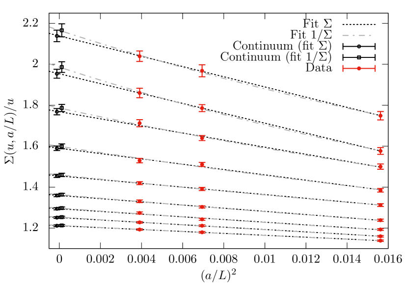
Figure 13: The bare coupling $g_{0}^{2}$ is fixed on several lattice sizes $L/a=8,10,12,16$ so that the renormalized coupling is equal to $\bar{g}^{2}=u_{i}$ for nine values $u_{i}\approx 2.12,2.39,2.73,3.20,3.86,4.49,5.30,5.86,6.54$. This means that all simulations have the same physical volume $L$, up to scaling violations. By computing the coupling on lattices twice as large, one determines a lattice approximation $\Sigma_{s}(u,a/L)$ of the step scaling function $\sigma_{2}(u)$. This plot shows the continuum extrapolation of the lattice step scaling function $\Sigma_{s}(u,a/L)$ (see Eq. (199)). The continuum values can be used to parameterize $\sigma_{2}(u)$ for $u\in[2.12,6.54]$, or to determine the $\beta$-function. (Source [161]).

By repeating a series of continuum extrapolations at different values of the coupling $u$, the function $\sigma_{s}(u)$ can be determined. Once the step scaling function is known, the RG problem is solved non-perturbatively. Note that the relation

$$\log s=-\int_{\sqrt{u}}^{\sqrt{\sigma_{s}(u)}}\,\frac{{\rm d}x}{\beta(x)}\,,$$ (200)

is exact. The determination of the $\Lambda$-parameter Eq. (16) uses the previous relation to break the fundamental integral of the $\beta$-function

$$\int_{0}^{\bar{g}(\mu_{\rm had})}\,\frac{{\rm d}x}{\beta(x)}\,,$$ (201)

into several pieces. The scale $\mu_{\rm had}$ is a low-energy scale, of the same order as the reference scale used to “set the scale”, as discussed in section 4.5.2. With the help of the step-scaling function one can produce a series of couplings $\bar{g}_{k}$ such that

$$\bar{g}_{0}^{2}\equiv\bar{g}^{2}(\mu_{\rm PT});\qquad\bar{g}_{k-1}^{2}=\sigma_{s}(\bar{g}^{2}_{k})\,.$$ (202)

Note that since the step scaling function changes the scale by a factor $s$, we have $\bar{g}^{2}_{k}=\bar{g}^{2}(s^{k}\mu_{\rm had})$. Recalling the basic relation Eq. (200) the integral of Eq. (201) can now be written as

$$\int_{0}^{\bar{g}(\mu_{\rm had})}\,\frac{{\rm d}x}{\beta(x)}=\int_{0}^{\bar{g}(s^{n}\mu_{\rm had})}\,\frac{{\rm d}x}{\beta(x)}+n\log s\,.$$ (203)

With moderate values of $n$ (i.e.$\,n\sim 10$) one can reach high energy scales, since $s^{n}\mu_{\rm had}\sim 100$ GeV. The remaining integral in Eq. (203) can be very well approximated by using perturbation theory (cf. section 3.2).

$$\int_{0}^{\bar{g}(s^{n}\mu_{\rm had})}\,\frac{{\rm d}x}{\beta(x)}\raisebox{-0.43057pt}{ $\stackrel{{\scriptstyle\small{n\to\infty}}}{{\sim}}$}\int_{0}^{\bar{g}(s^{n}\mu_{\rm had})}\,\frac{{\rm d}x}{\beta_{\rm PT}(x)}+\dots\,.$$ (204)

The scale $s^{n}\mu_{\rm had}$ is the scale at which the result is matched with perturbation theory

$$\mu_{\rm PT}=s^{n}\mu_{\rm had}\,.$$ (205)

One of the big advantages is that finite size scaling allows to vary this scale substantially: it can be pushed to very large values with a moderate computational effort. The $\Lambda$-parameter can be determined by matching with perturbation theory at different energy scales. We have already seen an example of such analysis in figure 3.

Direct determination of the $\beta$-function

Recent works use the step scaling function to directly determine the $\beta$-function. This approach has some technical advantages like making the determination of arbitrary ratios of scales $\mu_{1}/\mu_{2}$ possible, or allowing different scales factors $s$ to be used to fix the same set of coefficients. Several parametrizations are possible. At high energies the most natural one is just to write

$$\beta(x)=-x^{3}\sum_{n=0}^{N}b_{n}x^{2n}\,,$$ (206)

with the first few coefficients fixed by the perturbative prediction. In this case, once the $\beta$-function is known, one can use

$$\frac{\mu_{\rm PT}}{\mu_{\rm had}}=\exp\left\{-\int_{g(\mu_{\rm PT})}^{g(\mu_{\rm had})}\,\frac{{\rm d}x}{\beta(x)}\right\}$$ (207)

to connect the perturbative and hadronic scales similarly to Eq. (205).

Another advantage is that it allows a direct comparison of the data with perturbation theory by comparing the non-perturbatively determined $\beta$-function and its perturbative expansion (see [34, 161] for some examples).

6.7.3 Matching to an experimental quantity

In the previous section we have seen how finite size scaling techniques are able to solve non-perturbatively the RG equations: ratios of scales defined in a massless scheme, like $\mu_{\rm PT}/\mu_{\rm had}$ can be determined precisely. But what we really need are the values of these scales in physical units. Following the discussion of section 4.5.2, we need to determine $\mu_{\rm had}/M_{\rm ref}$, where $M_{\rm ref}$ is a reference scale (for example the $\Omega$ mass) determined in large volumes and with physical values of the quark masses (i.e. in a setup that can be matched with an experimental input).

In detail, the procedure is as follows: first one fixes the value of the coupling in a given massless finite volume renormalization scheme to some particular value

$$\bar{g}^{2}(\mu_{\rm had})=\text{fixed}\,,$$ (208)

for several values of $L/a$. Since the coupling depends only on one scale $\mu_{\rm had}\propto 1/L_{\rm had}$, the physical volume of all these simulations is the same, up to scaling violations (i.e. the different values of $L/a\propto 1/(a\mu)$ are really different values of $a$ at the same $L=L_{\rm had}$).

Second, one determines in large volume simulations the value of some low-energy scale at the same values of the bare coupling $g_{0}$ and for physical values of the quark masses. This low energy scale is typically whatever reference quantity is used to set the scale. For example let us assume that it is the mass of the $\Omega$ baryon $M_{\Omega}$. The large volume lattice simulations yield values of the mass in lattice units, we denote this dimensionless quantity $\hat{M}_{\Omega}(a)$ where we have written explicitly its dependence on the lattice spacing $a$. Since the bare coupling has been kept the same, the values of $a$ in our determination of $a\mu_{\rm had}=a/L_{\rm had}$ are the same, up to scaling violations, as the values of $a$ in our determinations of $\hat{M}_{\Omega}(a)$. This allows to determine the ratio

$$\frac{\mu_{\rm had}}{M_{\Omega}}=\lim_{a\to 0}\frac{a\mu_{\rm had}}{\hat{M}_{\Omega}(a)}\,.$$ (209)

Note that the fact that different values of the quark masses or physical volumes are used for the determination of $a\mu_{\rm had}$ and $aM_{\Omega}$ is not an issue once the continuum extrapolation is performed [49]. Once this ratio is known in the continuum, the experimental value of $M_{\Omega}$ can be used to determine $\mu_{\rm had}$ in physical units

$$\mu_{\rm had}=M_{\Omega}^{\rm exp}\times\frac{\mu_{\rm had}}{M_{\Omega}}\,.$$ (210)

We suggest the reader to look again to Fig. 11 for a schematic summary of the full procedure: the $\Lambda$-parameter, and therefore the strong coupling constant, is determined from just one experimental dimensionful quantity (like $M^{\rm exp}_{\Omega}$). Perturbation theory is only needed at scales larger than $\mu_{\rm PT}=s^{n}\mu_{\rm had}$. This scale can be made (almost) arbitrarily large with a modest (but dedicated) computational effort.

7 Present and future of lattice determinations of $\alpha_{s}$

Figure 14: Current uncertainty in the determination of the strong coupling. A 5% uncertainty in the three flavor $\Lambda$ parameter translates in a sub-percent precision in the strong coupling at the electroweak scale. Electromagnetic uncertainties in the scale (section 4.5.2) and charm quark effects (section 5) are far from being the limiting factor in the precision (note the gap in the axes). See text for more details.

In this review we have focused on the determination of the $\Lambda$-parameter, which in our opinion should be considered the fundamental parameter from which the strong coupling constant can be deduced. From our point of view it has several conceptual advantages, first and foremost the fact that it is defined non-perturbatively, and therefore allows a clean separation of the role of perturbation theory. Moreover since $\Lambda$ has units of mass, its connection with scale setting is transparent. Many determinations of the strong coupling claim a precision below 1%. This is impressive, but if translated to an uncertainty in the $\Lambda$-parameter the achievement looks quite modest compared with other state of the art lattice QCD computations: a 5% uncertainty in $\Lambda^{(3)}_{\overline{\rm MS}}$ is enough to achieve a 1% precision in $\alpha_{\overline{\rm MS}}(M_{Z})$. In an era where many lattice computations of decay constants, the hadron spectrum, or the anomalous magnetic moment of the muon reach a sub-percent precision, the current $\approx 5\%$ uncertainty in the $\Lambda$-parameter is a clear testimony to the difficulties involved in solving this multi-scale problem.

As a consequence many of the fine details needed in current state of the art lattice QCD computations are not crucial for improving the current determination of $\Lambda_{\overline{\rm MS}}$. Let us illustrate this point in detail by discussing the effect of electromagnetic corrections and massive sea quarks.

Electromagnetic effects

They enter in any determination of the strong coupling in two different ways.

First there are the electromagnetic effects in whatever quantity is used to set the scale. If the pion decay constant is used to set the scale, one can claim that these effects are of the order of $0.3\%$ in $f_{\pi}$ (see discussion in section 4.5.2). The size of this effect has been recently confirmed by numerical QCD+QED computations [77] (although with a smaller precision).The other popular choice for scale setting is the $\Omega$ baryon mass. Electromagnetic corrections in the $\Omega$ baryon have been computed recently via lattice QCD simulations and found to be significantly below 0.3% [162]. Since the relative error in the scale propagates into an equal relative error in $\Lambda$, the effects of the EM uncertainties in the scale will only affect the strong coupling at the $0.05\%$ level: well below the precision of any foreseeable result in the near future.

The second point where electromagnetic corrections affect the lattice determinations of the strong coupling is in the actual running. The running of the strong coupling is affected by the fact that quarks are electrically charged and couple to photons. These effects are estimated in perturbation theory (see for example [163] for a calculaiotn up to three loops) with the result that the leading effect is an $\mathcal{O}(\alpha_{s}\alpha_{EM})$ term that can be interpreted as a correction in the leading $b_{0}$ term of the $\beta$ function. This correction is below the percent level and translates in a per-mille effect in $\Lambda$, i.e. a completely negligible effect in $\alpha_{s}(M_{Z})$

Charm sea quark effects

Some lattice collaborations nowadays include a dynamical charm quark in their simulations (these simulations are usually labeled as $N_{\rm f}=2+1+1$), while other collaborations still ignore the effects of a dynamical charm quark ($N_{\rm f}=2+1$) . A naive estimate of the contribution of charm quark loops can be obtained from the large-$N_{c}$ counting rules, which suggest that quark loop effects are $1/N_{\rm c}$ suppressed. Moreover decoupling arguments show that these are further suppressed by a factor $(E/M_{c})^{2}$ where $E$ is the typical energy scale of an hadronic quantity, and $M_{c}$ is the RGI-invariant charm quark mass. For the sake of the argument we will take here $E\approx 0.4$ MeV (this corresponds to the energy scale of a typical hadronic scale like $r_{0},\sqrt{8t_{0}}\approx 0.5$ fm). Putting these pieces together we obtain

$$\frac{1}{N_{\rm c}}\times\left(\frac{E}{M_{c}}\right)^{2}\longrightarrow 3\%\,\text{effect}\,.$$ (211)

One can argue that there is an additional suppression by a factor $\alpha_{\overline{\rm MS}}(M_{c})$. In this case the overall effect will be $\mathcal{O}(1\%)$.

Either way, we have strong evidence that charm quark loop effects are dynamically suppressed, resulting in overall effects much smaller than the uncertainty quoted above.

• The FLAG report does not find any significant difference between lattice $N_{\rm f}=2+1$ and $N_{\rm f}=2+1+1$ computations in several quantities (decay constants, quark masses, …) [1]. Some of these computations agree with a sub-percent precision.

• Charm quark effects in dimensionless ratios of gluonic quantities (ie $r_{0}/\sqrt{t_{0}},w_{0}/r_{0},\dots$) have been estimated recently [102] by comparing $N_{\rm f}=2$ lattice simulations with two heavy quarks and the pure gauge theory. The measured effect is below the 0.4% level.

The previous considerations apply directly to the case of the determination of the strong coupling. The relative error in the scale (i.e.  $r_{0},t_{0},f_{\pi},\dots$) propagates linearly into $\Lambda$, and these effects are well below the $0.1\%$ uncertainty in $\alpha_{s}(M_{Z})$.

Charm quark effects also affect the decoupling relations used to translate $\Lambda_{\overline{\rm MS}}^{(3)}\to\Lambda_{\overline{\rm MS}}^{(4)}\to\Lambda_{\overline{\rm MS}}^{(5)}$, which are needed to quote the value of the strong coupling at the electroweak scale. The perturbative relations have non-perturbative corrections $\mathcal{O}(\Lambda^{2}/M_{c}^{2})$, and these effects have been recently estimated to be about $0.2\%$ [22]. This estimate is a result of comparing $N_{\rm f}=2$ lattice simulations with two heavy quarks and the pure gauge theory ($N_{\rm f}=0$). The same reference adds a factor two to this estimate, resulting in a conservative uncertainty in $\Lambda$ of about $0.4\%$. Again, this is well below our current precision.

In summary, it is useful to keep in mind that the precision in lattice determinations of the strong coupling is limited for reasons that are very different from the ones that limit other current lattice QCD computations.

In figure 15 we summarize the current status of the lattice and non-lattice determinations of the strong coupling. For the case of the non-lattice determinations we use the PDG [100] averages, which include phenomenological determinations from $\tau$-decays, DIS, QCD Jets, hadron collider data and electroweak precision fits. For the lattice results we use the FLAG averages .

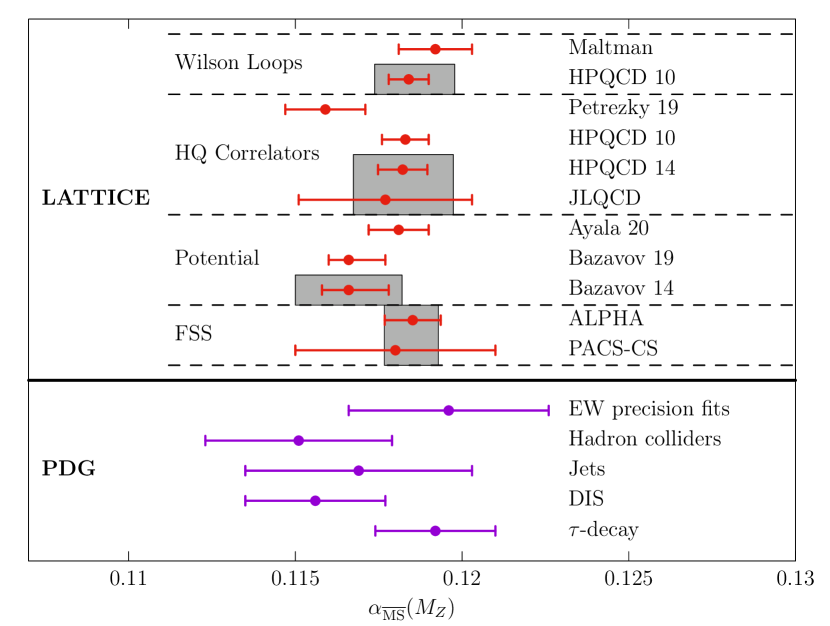
Figure 15: Summary of lattice and non-lattice result for the strong coupling using different methods. For non-lattice results we use the PDG averages [100]. For the lattice results we quote the works that enter in the FLAG average [1] and the recent updates that have been published after the FLAG review. The gray boxes are the FLAG average for each method. The recent updates (Petrezcky 19 [106] and Bazavov 19 [164]) are not included in the current FLAG averages because they were published after the FLAG update. See text for more details. (References: Maltman [165], HPQCD 10 [107], Petrezky 19 [106], HPQCD 14 [139], JLQCD [138], Ayala 20 [130], Bazavov 19 [164], Bazavov 14 [129], ALPHA [166], PACS-CS [156]).

Without duplicating the detailed work done in the FLAG review, in what follows we shall try to assess the limiting factors in the different extractions of the strong coupling. The first naive observation is that figure 15 does not include lattice results for some of the methods reviewed in section 6. Let us then begin by discussing these methods.

7.1 Methods not entering the FLAG average

FLAG applies several quality criteria to determine which works enter in the average. These quality criteria aim at covering all the possible sources of systematic effects in the calculation. Data sets that are unlikely to allow for a reasonable control of systematic effects are excluded from final averages. The methods that do not qualify to enter in the final average are discussed in this subsection.

QCD vertices

There are three lattice works in the latest FLAG review that extract the value of the strong coupling from QCD vertices [114, 115, 116]. In all cases the data set does not allow for a controlled continuum extrapolation, which prevents these works from contributing to the average. Another work [113] has appeared since the FLAG review was published, but the extraction of the strong coupling is still done from simulations at a single lattice spacing.

The limiting factor in these determinations is the ability to reach energy scales that are sufficiently high to make contact with perturbation theory while having the continuum extrapolation under control.

HVP

Two works extract the strong coupling from the vacuum polarization [143, 142]. Nevertheless these works do not qualify for the FLAG average because the continuum extrapolation is not under control.

Here we face the same issues: the difficulty to reach the perturbative region while having the continuum extrapolation under control.

Eigenvalues of the Dirac operator

There is only a single work that determines the strong coupling from the eigenvalues of the Dirac operator [144]. The extraction is performed at a very low energy scale, where $\alpha\approx 0.6-0.4$. According to the FLAG criteria, this does not allow to control the matching with perturbation theory.

All in all, these methods fail to show convincing evidence for a safe contact with the asymptotic perturbative behavior and/or fail to show that the continuum limit can be reached at the energy scales needed to extract the value of $\alpha_{s}$. At the time of writing, we think that it would be better to use the value of the strong coupling as an input to investigate the physics related with these phenomena, instead of using these physics effects to perform a precision determination of the fundamental parameters of the SM. Of course this situation might change in the future. More powerful computers might allow to reach higher energies. Eventually a safe contact with perturbation theory in the continuum can lead to precise values of $\alpha_{s}$, but this is not the case at the moment.

7.2 Methods that enter the FLAG average

Next we will comment critically on the methods that actually enter in the final FLAG average (see Fig. 15). These methods show compelling evidence of producing robust results in the continuum limit (by using several lattice spacing to extrapolate their results) and reach energy scales where the perturbative matching is convincing.

A crucial point in the following discussion is the estimate of the truncation error, i.e. the uncertainty that is introduced in the determination of the coupling by working at a given order in perturbation theory. As we shall see below, this is the main source of uncertainty in most of the determinations of the strong coupling . Here we will look at these uncertainties in detail using the scale variation method. In particular we will examine how a given measurement of an observable in three flavor QCD at a physical scale $Q$ produces different determinations of $\alpha_{\overline{\rm MS}}(M_{Z})$ when the ratio between the renormalization and physical scales is varied. Without loss of generality, we will assume that the observable is determined in $N_{\rm f}=3$ QCD and normalized as a coupling (as discussed at the beginning of section 6)

$$\alpha(Q)=\alpha_{\overline{\rm MS}}(sQ)+\sum_{k=2}^{n}c_{k}(s)\alpha_{\overline{\rm MS}}^{k}(sQ)\,.$$ (212)

The procedure that we employ to estimate the uncertainty in our determination of $\alpha_{\overline{\rm MS}}(M_{Z})$ is detailed in appendix B. The reader interested in numerical values should consult the freely available package https://igit.ific.uv.es/alramos/scaleerrors.jl. In summary we proceed as follows:

1. Fix the value $\alpha(Q)$ using a canonical value $\Lambda^{(3)}_{\overline{\rm MS}}=341\,{\rm MeV}$ (equivalent to $\alpha_{\overline{\rm MS}}(M_{Z})\approx 0.1185$) for some value of the scale $\mu=s_{\rm ref}Q$. This is achieved by reverse engineering, i.e. by computing

   $$\alpha(Q)=\alpha_{\overline{\rm MS}}(\mu)+\sum_{k=2}^{n}c_{k}(s_{\rm ref})\alpha_{\overline{\rm MS}}^{k}(\mu)\,,\qquad(\mu=s_{\rm ref}Q)\,.$$ (213)

   where $\alpha_{\overline{\rm MS}}(\mu)$ is the value of the three flavor coupling at scale $s_{\rm ref}Q$ obtained from $\Lambda^{(3)}_{\overline{\rm MS}}=341$ MeV.

2. Use Eq. (212) again, in order to determine the values of $\alpha_{\overline{\rm MS}}(sQ)$, by solving

   $$\alpha(Q)=\alpha_{\overline{\rm MS}}(sQ)+\sum_{k=2}^{n}c_{k}(s)\alpha_{\overline{\rm MS}}^{k}(sQ)\,.$$ (214)

   at the values $s=s_{\rm ref}/2,2s_{\rm ref}$.

3. Use the 4- and 5-loop $\beta$-function to run the values of $\alpha_{\overline{\rm MS}}(sQ)$ obtained in step 2. to the reference scale $M_{Z}$ (crossing the charm and bottom thresholds). A comparison between the values of $\alpha_{\overline{\rm MS}}(M_{Z})$ is a measure of the truncation uncertainty due to the scale variation.

Observable	loops	$Q$ [GeV]	FLAG error [%]	$\delta_{(4)}^{\star}\,[\%]$	$\delta_{(2)}\,[\%]$	$\delta_{(2)}^{\star}\,[\%]$
		1.5	1.4		2.6	2.7
Potential	4	2.5		0.9	1.5	1.5
		5.0		0.4	0.8	0.8
HQ $r_{4}$		$m_{\rm c}$	1.3		2.7	2.8
HQ $r_{4}$	3	$2m_{\rm c}$		1.2	1.5	1.6
HQ $r_{6}$		$2m_{\rm c}$			2.3	1.2
HQ $r_{8}$		$2m_{\rm c}$			2.8	4.8
$-\log W_{11}$	3	4.4	1.0	2.8	3.3	2.5
$-\log W_{12}/u_{0}^{6}$		4.4		3.5	3.2	3.1
FSS	3	80		0.1	0.2	0.2

Table 4: Summary of truncation uncertainties on $\alpha_{\overline{\rm MS}}(M_{Z})$ estimated by varying the scale. We compare the error quoted by flag with a change of scale by factors two and four around $s=1$ or $s=s^{\star}$ (the value of fastest apparent convergence). For each method we quote the number of known loops in the relation between the observable and the $\overline{\rm MS}$ scheme according to h counting in section 6. Details on the different types of extractions can be found in section 7.2.2 (potential), section 7.2.3 (HQ), section 7.2.4 ($\log W_{11},\log W_{12}$) and section 7.2.1 (FSS).

The usual procedure in phenomenology is to vary the renormalization scale by a factor 2 above and below some reference scale. Estimates of the truncation uncertainties that use renormalization scales below 1 GeV tend not to be reliable. Since many extractions of the strong coupling are performed at relatively low scales, the above mentioned procedure might lead to unreasonable uncertainties. For this reason, the uncertainty resulting from comparing the change $s_{\rm ref}\to 2s_{\rm ref}$ provides complementary information on the size of the truncation uncertainties, specially if one explores the dependence with $s_{\rm ref}$ in a range $1-2$. In order to get a more quantitative understanding of these effects, we will use the following quantities.

$\delta_{(4)}(s_{\rm ref})$:

Change the renormalization scale by a factor two above and below some reference scale $s_{\rm ref}Q$. We quote a symmetric error by averaging the difference between the scales $s_{\rm ref}Q$ and $2s_{\rm ref}Q$, and the difference between the scales $s_{\rm ref}/2Q$ and $s_{\rm ref}Q$. Note however that in some cases the error is markedly asymmetric.

$\delta_{(2)}(s_{\rm ref})$:

Change the renormalization scale by a factor two above the reference scale $s_{\rm ref}Q$ only.

We will show explicitly in the computations below how the two measures $\delta_{(4)}(s_{\rm ref})$ and $\delta_{(2)}(s_{\rm ref})$ depend on the choice of $s_{\rm ref}$. In principle any number $\mathcal{O}(1)$ is a reasonable choice for $s_{\rm ref}$, but there can be significant differences in the results depending on its actual value. For this reason we will explore two common choices.

• Take $s_{\rm ref}=1$. i.e.  the renormalization and physical scales are the same. In this case the uncertainties will be labeled $\delta_{(2)},\delta_{(4)}$.

• Take $s_{\rm ref}=s^{\star}$ as the value of fastest apparent convergence. This value is determined with the condition

  $$c_{2}(s^{\star})=0$$ (215)

  i.e. the NLO coefficient in the relation between $\alpha(Q)$ and $\alpha_{s}$ vanishes (see Eq. (212)). In this case the uncertainties will be labeled $\delta^{\star}_{(2)},\delta^{\star}_{(4)}$.

A summary of the results is presented in table 4. One can readily see that the truncation uncertainties obtained with this method are in the same ballpark as the FLAG uncertainties, except for the case of the Wilson loops, where our estimates are substantially larger. Once again we would like to end with a warning: estimates of the truncation uncertainties based on the scale variation can (and have been shown to) fail in some cases (see discussion in section 3.2 and specifically figure 3).

7.2.1 Finite size scaling

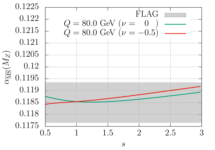
(a)

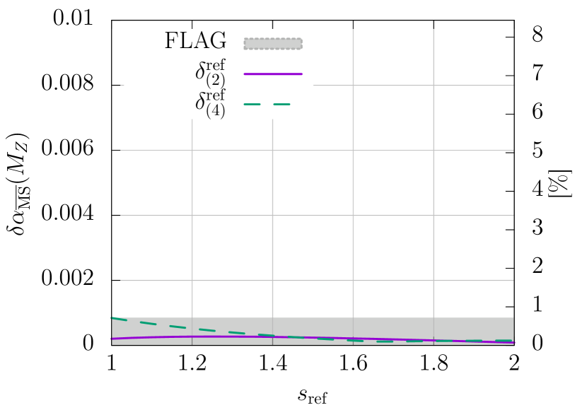
(b)

Figure 16: Truncation effects in $\alpha_{s}$ extractions from finite size scaling. Note that in this methods the extraction is performed at very high energies $Q\approx 80$ GeV. The scale dependence of the coupling at $Q=8$ GeV in plot (a) is just for reference. Plot (b) shows that truncation uncertainties are typically much smaller than the quoted uncertainties.

The FLAG average is the result of Refs. [156, 166], wich are in good agreement with each other. Perturbation theory is used at very high energies ($Q\approx 80$ GeV), where perturbative estimates of the truncation uncertainties are reliable. They affect the extraction of $\alpha_{s}$ only at the $0.1-0.2\%$ level (see figures 16), well below the quoted uncertainties.

The most recent work [166] explores the dependence of the extractions of $\Lambda$ on the physical energy scale over a large range of energy scales $Q\sim 4-140$ GeV (see Figure 3 and the related discussion). This study compares their extraction of the coupling $\alpha_{s}$ with the extraction performed with several observables after extrapolating the renormalization scale at which perturbation theory is used $\mu\to\infty$ (see discussion in section 3.2). All in all, results based on finite size scaling do not depend on estimates of the perturbative uncertainties done in perturbation theory, although figure 16 show that they tend to be rather small, as expected given that the electroweak scale is reached by non-perturbative simulations. We should also point to the detailed study in [35].

The continuum extrapolation is the main source of systematic uncertainty. According to our discussions in sections 4.5 and 6.7 the method allows to to perform a controlled continuum extrapolation by using several values of the lattice spacing at each energy scale. In particular, the most delicate continuum extrapolations in [161] uses three values of the lattice spacing that vary by a factor two at each value of the scale.

The statistical precision of the non-perturbative running is the main limiting factor of these determinations. Note that coupling definitions using the gradient flow – see section 4.5.3 and 6.7 – have a very small variance. These couplings have been used in Ref. [166], but not in Ref. [156] (these techniques were not known at the time), explaining the large difference in the error between the two works: the result in [156] quotes a 2.5% error in $\alpha_{\overline{\rm MS}}(M_{Z})$, while the result [166] quotes a 0.7% uncertainty.

7.2.2 Static potential

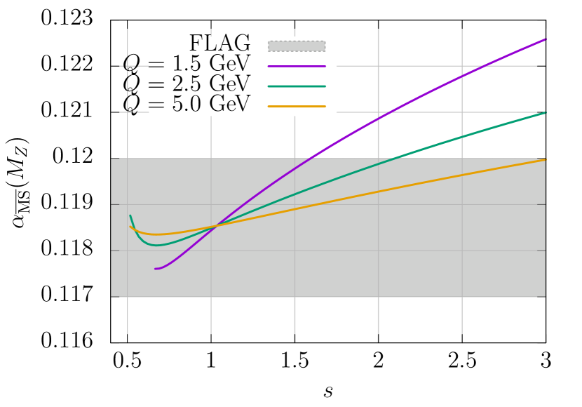
(a)

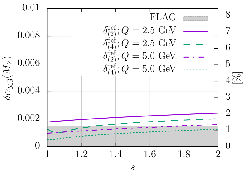
(b)

Figure 17: Truncation effects in $\alpha_{s}$ extractions from the static potential. Note that the high energy scale $Q=8$ GeV is only reached in the last work [164]. The FLAG error is determined for

The FLAG average is basically the result of Ref. [129] with an added uncertainty because of the perturbative truncation errors. Since the publication of the FLAG report, two new determination of the strong coupling by the same group has been published [164, 130]. In these last works the determination of the strong coupling is extracted at energy scales $Q\approx 2.5-8$ GeV, improving significantly the previous determination, which used $Q\in 1.4-4.9$ GeV. Energy scales $\approx 5$ GeV can be reached with several values of the lattice spacing. On the other hand the largest energy scales are reached at a single lattice spacing, preventing a proper continuum extrapolation. The strong coupling is typically extracted from fits using energy scales about $2.5$ GeV and above.

We should recall that the simulations at very fine lattice spacing have a relatively small volume and are performed at fixed topology (see discussion in section 6.2), and in relatively small physical volumes.

In what follows we will focus on the truncation uncertainties. In our analysis we ignore the logarithmic corrections due the IR divergences of the static potential. This is partially justified: if one takes the logarithms as constants, truncation uncertainties as estimated below show only a mild variation (see appendix B.2). Nevertheless there is some concern here, since the natural scale at which the terms $\log\alpha$ are evaluated (the ultra-soft scale) is significantly smaller (see discussion in section 6.2).

Figure 17 shows the scale dependence of the strong coupling and the truncation errors $\delta_{(2)}^{\rm ref},\delta_{(4)}^{\rm ref}$ as a function of $s_{\rm ref}$. First it is important to point out that the error estimate by FLAG, even if it comes from a completely different argument is in the same ballpark as our estimates. For the relevant energy scales used in present works [129, 164] ($Q\in 1.4-5$ GeV) the perturbative estimates of the truncation uncertainties are in the range $\delta\alpha_{\overline{\rm MS}}(M_{Z})\approx 2.6\%-0.8\%$, while the FLAG estimate of the truncation uncertainties is 1.4% (the most recent work [164] had not appeared at the time the FLAG review was published).

It is interesting to consider in detail the analysis of Refs. [129, 164, 130].

Ref. [129]:

The perturbative truncation error is estimated by changing the renormalization scale a factor $\sqrt{2}$ above and below the physical scale. Their result

$$\alpha_{\overline{\rm MS}}(M_{Z})=0.1166_{-0.0008}^{+0.0012}\,,$$ (216)

has an uncertainty between $-0.7\%$ and $+1\%$, that is actually dominated by the perturbative truncation uncertainty. This uncertainty is smaller than the quoted uncertainty by FLAG ($1.4\%$).

Ref. [164]:

The estimate comes from a similar analysis, but this time the renormalization scale is varied a factor 2 above and below the physical scale. Moreover they also include in their estimate the effect of the different treatment of the logarithmic corretions in the perturbative expansion (that we have ignored in our analysis). This is very similar to our approach, and the uncertainty is similar to our quoted $\delta_{(4)}$ in table 4, with the exception that they do not symmetrize the error. Their result

$$\alpha_{\overline{\rm MS}}(M_{Z})=0.1166_{-0.0006}^{+0.0011}\,,$$ (217)

has a very similar uncertainty than the previous work, see Eq. (216), despite the fact that they reach significantly higher energies. Obviously this is a result of the more conservative approach to the estimate of the truncation uncertainties.

Reference [164] claims that if they would have followed the same recipe as in reference [129], their updated result Eq. (217) would have the uncertainty reduced by a factor two.

Ref. [130]:

This work uses the same data as reference [164], but they use the known terms in the perturbative series to fix the normalisation of the renormalon ambiguity and subtract some non-perturbative (i.e.  power) corrections. Their final result

$$\alpha_{\overline{\rm MS}}(M_{Z})=0.1181(9)\,,$$ (218)

quote a similar uncertainty as [164], but their central value is significantly larger.

In summary, the estimate by FLAG of these uncertainties (1.4%) is reasonable. It is basically the same as the difference in central values between the two most recent works [164] and  [130], that use the same data but different strategies to match with perturbation theory. This uncertainty is also larger than the total quoted uncertainty in both works [130, 164].

Determinations of the strong coupling from the static potential have recently improved significantly. Also the estimate of perturbative uncertainties is more conservative compared with previous works. These determinations are in very good shape, but the following points should be better understood:

• The most important point to be understood is if the perturbative region is reached in current extractions. The significant difference in central values between extractions using the same dataset but different power corrections (i.e.  Refs. [130, 164]) needs a better understanding.

  This difference between central values is about $1.4\%$, similar to the uncertainties that we obtained from a simple scale variation approach. We emphasize that our estimate does not address the issue of the logarithmic corrections to the perturbative series, related with the IR divergences of the static potential.

• Another manifestation of the same problem is the strong dependence on the value of $\Lambda^{(N_{\rm f}=0)}$ that has been observed for extractions based on the static potential for values of the coupling $\alpha^{3}_{s}\lesssim 0.01$ [168]. This effect has been studied in [164] and they observe a much milder effect.

  Note however that in this last reference $\Lambda$ is extracted as a fit over a range of energy scales. This procedure makes it much more difficult to see any dependence in the extracted value of $\Lambda$, and in fact means that all the different extractions of $\Lambda$ (with the exception of one point) use data with $\alpha^{3}>0.01$.

• The effect of the bad sampling of the topological charge has still to be investigated in detail. The ensembles at the finest lattice spacing have the topology completely frozen (see [169]). The impact of frozen topology can be studied by computing the scale $r_{1}$ from ensembles that are stuck in distinct topological sectors. The numerical results so far are all compatible within errors. Note however that the values of the topological charge simulated (basically 2 and 0) are small. A dedicated quenched study could shed some light on these issues.

• A related problem is that the physical volumes are relatively small (with $m_{\pi}L\approx 2.2$), and the effect of this small volumes on the determination of the scale and the static force is unclear. On general grounds, the static force is a short distance observable and one expects finite volume effects to be very small. Probably the largest source of finite volume effects are in the scale determination $r_{1}$, but one should keep in mind that the uncertainty in the scale has a small effect on the uncertainty of $\alpha_{s}(M_{Z})$. It would be interesting to quantify at which level of precision finite volume effects start to be a concern for these determinations.

7.2.3 Heavy quark correlators

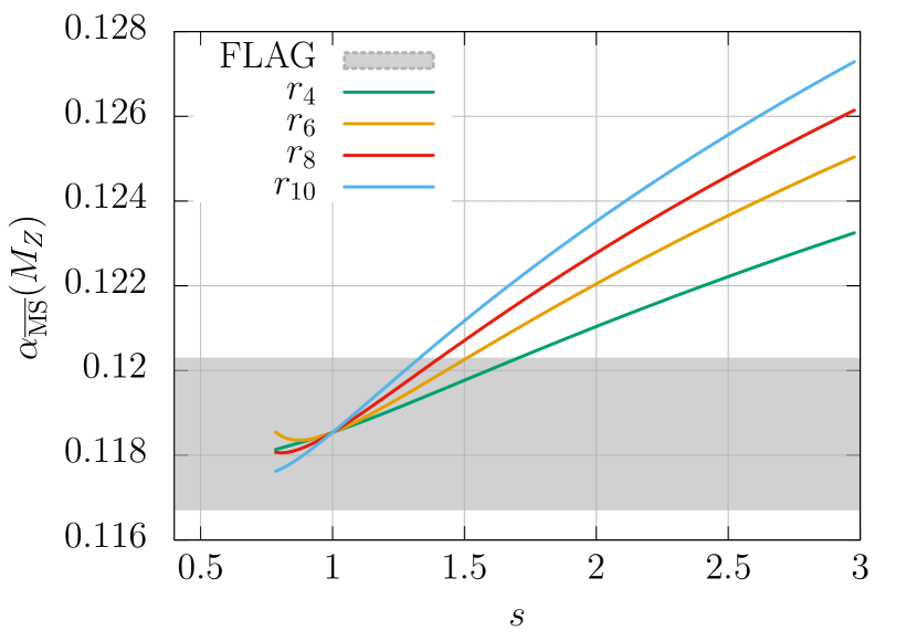
(a)

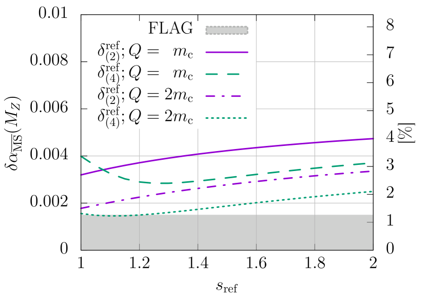
(b)

Figure 18: Truncation effects in $\alpha_{s}$ extractions from heavy quark correlators.

The average in figure 15 is the result of the works [107, 139, 138]. Once again the most delicate sources of uncertainty are the perturbative error and controlling the continuum extrapolation. It is instructive to see how different works estimate that particular systematic error.

JLQCD collaboration [138]:

The authors use a scale variation method, very similar to our procedure (see figure 18). A crucial difference is that they vary independently both the renormalization scale in the quark mass and in the strong coupling in the range $2-4$ GeV (this typically increases the estimates of the uncertainties). Also this work does not use the moment $r_{4}$. This is the quantity with the best perturbative behavior (see figure 18), but they find the continuum extrapolation very challenging. Their result

$$\alpha_{\overline{\rm MS}}(M_{Z})=0.1177(26)\,,\qquad[2.2\%]\,,$$ (219)

claims a $\sim 2\%$ error, mostly dominated by the perturbative truncation uncertainties.

Ref. [137]:

They estimate the truncation uncertainty by estimating the $\alpha^{4}(\mu)$ term in the perturbative expansion of $r_{n}$. They use a range of values $c_{3}(1)=\pm 2c_{2}(1)$ (see Eq. (212)), which yields a perturbative truncation uncertainty that is much smaller than the one obtained by the scale variation method. The truncation uncertainty represents a negligible contribution to the uncertainty of their final result

$$\alpha_{\overline{\rm MS}}(M_{Z})=0.11622(84)\,,\qquad[0.7\%]\,,$$ (220)

which is 3 times more precise than the JLQCD result.

Ref. [106]:

This work can be considered an update of [137]. Again the perturbative uncertainty is computed by estimating the size of the $\mathcal{\alpha}^{4}(\mu)$ term in the perturbative expansion of $r_{n}$, but this time they allow a larger range of values for the unknown coefficient $c_{3}(1)=\pm 5c_{2}(1)$ (see Eq. (212)). Their updated result

$$\alpha_{\overline{\rm MS}}(M_{Z})=0.1159(12)\,,\qquad[1.0\%]\,,$$ (221)

has in fact a larger uncertainty.

Ref [139]:

The HPQCD collaboration analyze data close to the physical charm quark mass ($Q=m_{\rm c}$). Their analysis includes higher order terms in the perturbative expansion of their data amongst the fitted parameters. These unknown terms (up to powers $\alpha^{15}$) are constrained using Bayesian priors. The perturbative truncation errors are the main source of uncertainty, but their final result

$$\alpha_{\overline{\rm MS}}(M_{Z})=0.11822(74)\,,\qquad[0.6\%]\,,$$ (222)

claims an uncertainty 4 times smaller than our estimates of the truncation uncertainties at the scale $Q=m_{\rm c}$. This uncertainty is estimated by varying the number of terms added to the fit. It is not clear to the authors why this estimate should be a reliable estimate of the truncation uncertainties. In particular these error estimates are substantially smaller than the usual estimates coming from scale variation.

FLAG quotes a 1.2% truncation uncertainty for extractions performed at the scale $m_{\rm c}$. Our scale variation method tends to point to even larger values for the truncation uncertainty (see figures 18): about 2-3% for extractions at $m_{\rm c}$ and between 1-2% for extractions at $2m_{\rm c}$.

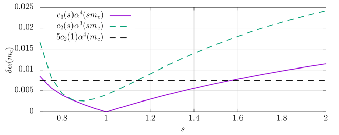
Figure 19: Truncation effects in $\alpha_{s}$ extractions using the last term in the perturbative series. The horizontal dashed line represent the estimate of Ref. [106] $\delta\alpha=5c_{2}(1)\alpha^{4}(m_{\rm c})$. This uncertainty is significantly smaller than the last known term in the series (dashed curve) unless the renormalization scale is chosen very close to the physical scale (i.e.  $s\approx 1$). This estimate is also smaller than the naive estimate coming only from the scale dependence of $c_{3}$ (solid curve).

It is easy to see why the estimates based on the value of the unknown coefficient $c_{3}(1)$ lead to small uncertainties. The last known coefficient in the series is given by

$$c_{2}(s)=0.0796+0.588\log(s)+2.052\log^{2}(s)\,.$$ (223)

This coefficient is anomalously small for $s=1$. Even when multiplied by a factor 5, it leads to a small estimate for the coefficient $|c_{3}|\approx 0.4$. On the other hand $c_{3}(s)$ can be estimated by other means. The scale dependence of $c_{3}(s)$ is fully predicted by the RG equations

$$c_{3}(s)=c_{3}(1)+0.865\log(s)+2.425\log^{2}s+2.939\log^{3}s\,.$$ (224)

(i.e.  only the non-logarithmic dependence $c_{3}(1)$ is unknown). This logarithmic dependence alone predicts a coefficient $|c_{3}(s)|\approx 3$ for even modest values of the scale $s=2$. This value for the $c_{3}$ term is 7.5 times larger than the estimate used in the last work Ref. [106] and almost 20 times larger than the estimate of [137]. There is an extra suppression $\alpha_{s}^{4}(sQ)$ that makes the uncertainty smaller when $s>1$, but this effect can only account for a factor between 2.8 (for $Q=m_{\rm c}$) and 4.5 (for $Q=2m_{\rm c}$): clearly insufficient to compensate the factor 7.5 or 20 in the estimate of $c_{3}$. Moreover, note that this simple estimate of $c_{3}(s)$ neglects completely $c_{3}(1)$. (See Figure 19). This explains why uncertainties based on scale variation are generally larger. Even assuming that one order more is known, and that $c_{3}(1)=0$, the scale variation approach results in $\approx 1.5\%$ error for $r_{4}$ at the charm scale.

Estimates of the truncation uncertainties based on varying the number of fit parameters constrained by priors and using Bayesian methods lacks a solid theoretical basis. We suggest that estimates based on scale variation should be preferred.

These considerations, together with the complicated scaling violations (see discussion in section 6.3) make it very challenging to obtain $\alpha_{s}$ with less than a 1.5% uncertainty using these methods. Quark masses significantly larger than the physical charm quark mass would be required (and one would need to deal with complicated continuum extrapolations).

There are two interesting directions for future research. First, the next order in the perturbative relation of the heavy quark moments could be very useful in future extractions. Second a dedicated pure gauge study, where significantly larger energy scales could be explored, would shed some light on the difficulties associated with the truncation uncertainties and the approach to the continuum in this type of lattice determinations.

7.2.4 Observables at the cutoff scale

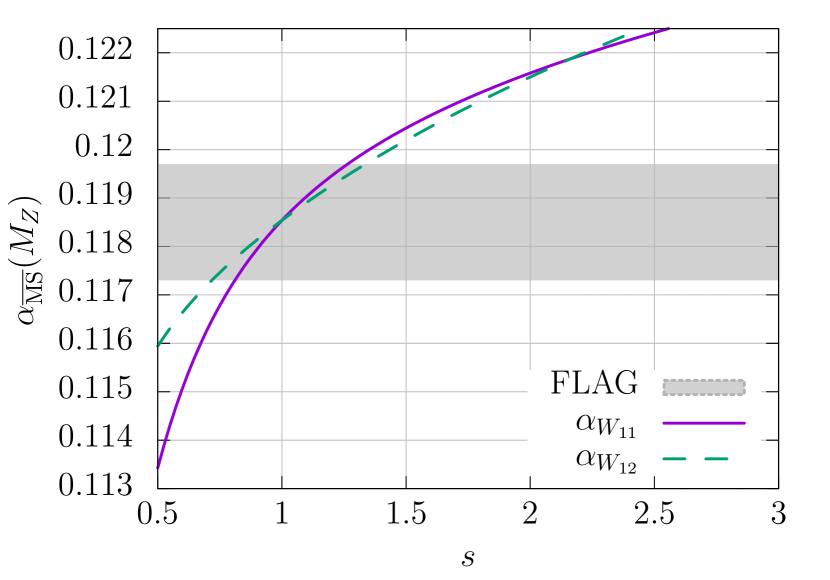
(a)

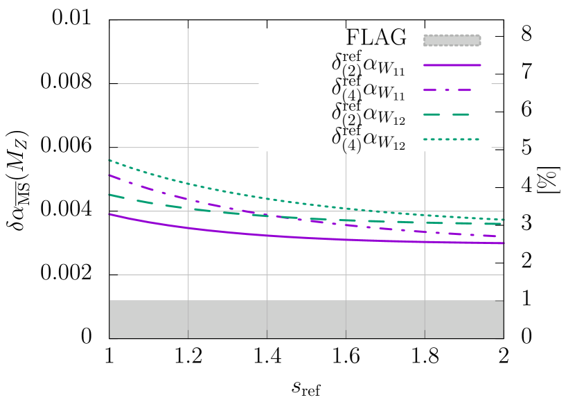
(b)

Figure 20: Truncation effects in $\alpha_{s}$ extractions from quantities at the scale of the cutoff.

There are two studies that contribute to this average [165, 107]. The main contribution to the uncertainty in these determinations is purely systematic, with the perturbative uncertainties playing a leading role. Note that an advantage for these observables is that there is no need to perform a continuum extrapolation. It is very difficult to obtain an independent estimate of the truncation uncertainties for these observables. The reason is that the data does not follow the known perturbative prediction in the range of energy scales reached in the numerical simulations [165, 107]. Several terms are added to the perturbative expansion, up to terms $\alpha^{10}_{\rm V}$ (see Eq. (175)), and the higher-order coefficients are fixed by fitting the lattice data to the expression

$$\alpha_{W_{nm}}(1/a)=\alpha_{{\rm V}}(\mu)+c_{2}\alpha_{{\rm V}}^{2}(\mu)+c_{3}\alpha_{{\rm V}}^{3}(\mu)+\sum_{k=4}^{10}d_{i}\alpha_{{\rm V}}^{i}(\mu)\,.$$ (225)

Here $\alpha_{\rm V}$ is the coupling in the potential scheme (see Ref. [140]) and $\mu\approx\pi/a$ with the exact value depending on the observable). A crucial point in these extractions is the discretization used. We will focus in the same discretization as used in the works [170, 107].

At least one extra term, with an unknown coefficient, is necessary in order to obtain a satisfactory description of the data. Moreover, the data is not precise enough to determine all the extra coefficients, so Bayesian priors are used in order to constrain the size of the coefficients $d_{i}\approx 0\pm 2.5$. The HPQCD analyses [107] estimate the perturbative truncation error by varying the number of terms in expression Eq. (225). Firstly let us note that the perturbative expansion of $\alpha_{W_{nm}}$ is only expected to be asymptotic. In particular the coefficients in the perturbative expansion should eventually grow. Constraining the size of all coefficients to the same size $\mathcal{O}(1)$ is not justified based on theoretical arguments.

Following the exact same procedure that we used for the other observables, we can estimate the truncation error by performing a scale variation analysis. For this purpose, we describe the observable using the known perturbative coefficients in the perturbative expansion in terms of the renormalized $\overline{\rm MS}$ coupling:

$$\alpha_{W_{nm}}(1/a)=\alpha_{{\overline{\rm MS}}}(\mu)+c_{2}\alpha_{{\overline{\rm MS}}}^{2}(\mu)+c_{3}\alpha_{{\overline{\rm MS}}}^{3}(\mu)+\dots\,,$$ (226)

with $\mu\approx 2.4/a$ (the exact relation depending on the concrete quantity). For illustration, let us focus here on the shortest distance object (the plaquette), and the $1\times 2$ Wilson loop with tadpole improvement:

$$\alpha_{W_{11}}(a) =-\frac{1}{c_{1}^{(11)}}\log W_{11}=\alpha_{V}(d/a)+\frac{c_{2}^{(11)}}{c_{1}^{(11)}}\alpha_{V}^{2}(d/a)+\frac{c_{3}^{(11)}}{c_{1}^{(11)}}\alpha_{V}^{3}(d/a)+\dots$$ (227)

$$\alpha_{W_{12}}(a) =-\frac{1}{c_{1}^{(12)}}\,\frac{\log W_{12}}{u_{0}^{6}}=\alpha_{V}(d/a)+\frac{c_{2}^{(12)}}{c_{1}^{(12)}}\alpha_{V}^{2}(d/a)+\frac{c_{3}^{(12)}}{c_{1}^{(12)}}\alpha_{V}^{3}(d/a)+\dots\,.$$ (228)

These quantities show a very strong dependence on the scale (see figures 20), pointing to truncation uncertainties of the order 3%.

FLAG uses the HPQCD fit result, $d_{4}\approx 2$, to estimate the truncation uncertainty as $2\alpha^{4}$. This procedure results in a smaller value than the one obtained form the scale variation approach

$$\delta\alpha_{\overline{\rm MS}}(M_{Z})\approx 0.0012\,,\qquad[1\%]\,.$$ (229)

This last uncertainty is about 2.5 times larger than the estimate of HPQCD.

A last piece of information comes from comparing the results in Refs. [165, 170]. They use basically the same dataset (reference [165] uses a subset of the 22 quantities used in [170]), but analyse it using different perturbative expressions and deal with the non-perturbative corrections in different ways. Their results for $\alpha_{\overline{\rm MS}}(M_{Z})$ differ by a 0.6%–1.2%.

The overall conclusion is that truncation uncertainties based on varying the number of terms constrained with Bayesian priors underestimate significantly the true uncertainties. The same phenomena have been observed in the case of determinations based on currents of heavy quark correlators. Moreover it is important to recall that the lattice data for these short distance quantities do not follow the perturbative prediction if only the known coefficients are used, making it mandatory to fit several additional terms in the perturbative expansion constrained by Bayesian priors. We think that this method needs further study. In particular it is mandatory to find a solid estimate of the truncation uncertainties based on the same techniques that are common in the estimates of the perturbative QCD uncertainties. A detailed study in pure gauge could shed some light on the issue. Without these insights the claimed uncertainties of some of these computations (0.6%) seem an underestimate of the true uncertainties.

7.3 An opinionated and critical summary

What can we conclude on the status of the lattice determinations of the strong coupling? First we should only consider extractions with a dataset that allows a proper control over the different sources of systematic effects. This is the approach taken for example by the FLAG review. For the particular case of the determination of the strong coupling, the most delicate points in the extractions of the strong coupling is the estimate of the uncertainties related with the truncation of the perturbative series and the large scaling violations in short distance quantities. Note that controlling both sources of systematic uncertainties is challenging: cutoff effects are larger for short distance quantities, while perturbative truncation errors are larger for low energy quantities, the window problem described in section 2.2.3 is again the limiting factor. This is why we have insisted on these points along the review.

Many lattice methods do not allow a simultaneous control of these two sources of systematic effects with current computer resources. Typically in these cases the extractions of the strong coupling are performed at a single lattice spacing, and/or the extraction is performed at energy scales where significant contribution from non-perturbative effects are present. Our analytic understanding of these effects is, at best, very limited. In practical terms we have to deal with them by fitting these contributions. This is very delicate, since distinguishing the perturbative running from the non-perturbative contributions when the data is available only in a restricted range of scales is far from easy. We therefore prefer to focus on methods where the data follows the perturbative prediction and non-perturbative corrections are smaller than the uncertainties.

Still, with this ambitious aim, several methods that allow a reliable extraction the strong coupling have been developed in lattice QCD. These methods differ in their control over the systematic errors associated with the continuum extrapolation and the truncation uncertainties.

• Finite size scaling is the only method that offers a solution to the window problem instead of trying to find a compromise. Arbitrarily large energy scales can be reached, and the continuum extrapolation can be performed by using several lattice spacing at each constant renormalization scale.

  This strategy trades the systematic errors associated with the truncation of the perturbative series at relatively low scales with the statistical error accumulated when computing the non-perturbative running. It remains challenging to obtain precise results, but thanks to several recent developments, a sub-percent precision has been reached by these kind of determinations. The truncation uncertainties are negligible, since perturbation theory is typically applied at the electroweak scale. Several observables have been studied non perturbatively and in some cases agreement with perturbation theory is achieved over a large range of scales (from 4 to 140 GeV) [35, 166].

  Our reservation with this approach is that until now only two groups have used it to determine the strong coupling, and with very similar setups. A new independent determination would be welcome.

• Determinations based on the static potential have several advantages over most other determinations. First, the relevant perturbative relations are known to N³LO, one order more than what is typically known for other observables. Second, the non-perturbative lattice data seems to follow the perturbative prediction for energy scales as low as 2 GeV. This energy scale can be reached at several values of the lattice spacing and the data can be extrapolated to the continuum.

  At the moment of writing, two new studies [164, 130] have been published. One of them can be considered an update of some of the works evaluated by FLAG. This new determination improves significantly in the energy scales that they are able to reach. What is more important, they treat the perturbative uncertainties more conservatively than in previous works and claim a sub-percent precision in the strong coupling. The other recent work (Ref. [130]) uses the same dataset but a different treatment of the lattice data and matching with perturbation theory. They obtain a result for $\alpha_{\overline{\rm MS}}(M_{Z})$ about 1.3% larger, rising some doubts on the claimed sub-percent accuracy of these works.

  According to our analysis using the scale variation approach, the uncertainty quoted by FLAG is reasonable, although our method neglets the delicate issue of logarithmic corrections to the perturbative series.

  As with all large volume determinations, there are reservations with this method beyond the estimates of perturbative uncertainties, related with the compromises that are made. Determinations reach high energy scales (up to 8 GeV), but the energy scales where the continuum limit can be taken with several values of the lattice spacing are substantially lower. Some of the volumes simulated are relatively small ($m_{\pi}L\approx 2.2$). Moreover some of these simulations are affected by the problem of topology freezing, potentially making difficult to asses the statistical errors correctly. The range of scales where the methodology can be tested is limited, and we should always remember that truncation uncertainties estimated within perturbation theory can be misleading (see section 3.2), even when a conservative approach is taken. These points should (and will) be investigated further, but beyond any doubts determinations coming from the static potential have reached a considerable level of maturity and precision.

• Some extractions based on currents of heavy quark correlators are among the most precise determinations of the strong coupling. Scaling violations have a complicated functional form, but at least the continuum limit can be explored with several lattice spacing. On the other hand, and compared with extractions based on the static potential, our current perturbative knowledge in these extractions is one order less and cutoff effects seem larger. In summary, this method is more challenging than the static potential from both sides of the window problem. Most of the determinations are performed at the charm quark mass $M_{\rm c}$ GeV. At these low scales, truncation uncertainties estimated using the scale variation method are about $2-3\%$ in $\alpha_{\overline{\rm MS}}(M_{Z})$. The FLAG 2019 review quotes a smaller uncertainty ($1.5\%$). Some works claim a sub-percent precision, but we find it difficult to consider these estimates reliable.

  There are several directions in which these extractions can improve. First, it should be possible to extend the current perturbative knowledge by one order more. Second, this method has never been studied in detail in the pure gauge theory, where one could reach energy scales significantly larger than $M_{\rm c}$ with full control over the continuum extrapolations. In any case, until the perturbative knowledge is known and larger energy scales have been studied, it seems difficult to claim a smaller uncertainty than what the FLAG review assigns to these extractions.

• Finally, there is still work to do in order to better understand the determinations based on lattice observables defined at the cutoff scale. Despite these methods claiming the smallest uncertainties, this claim is not backed up by a solid analysis of the truncation uncertainties. A scale variation approach points to significantly larger uncertainties. In fact the truncation uncertainties in these extractions seem to be significantly larger when using several different methods. Our numerical investigation suggests that even the FLAG error is still underestimating this source of systematic uncertainty.

  One should also point out that in pure gauge there is a significant discrepancy between some recent extractions based on observables defined at the cutoff scale and a recent extraction using finite size scaling (see [171]).

Let us end this section with a general comment about figure 15. Basically every method to extract the strong coupling using lattice QCD seems to be able to reach a better precision than any phenomenological extraction. This seems at least in some cases, to be fully justified based on the general principles on which we have insisted along the review: the most precise phenomenological determination, the extraction of $\alpha_{s}$ from $\tau$ decays, is performed at a fixed energy scale $m_{\tau}\approx 1.7$ GeV. Larger energy scales cannot be probed in these extractions, while the perturbative expansion of the observable is known at the same order as in the extractions based on the static potential, where energy scales $\mu\approx 5$ GeV can be explored at several values of the lattice spacing. In finite size scaling the perturbative knowledge is one order less, but perturbation theory is applied at the electroweak scale and consistency of the results is checked in the energy range $4-140$ GeV for a one-parameter family of observables.

7.4 The future of lattice determinations of $\alpha_{s}$

Now that we understand the main limitations of the different lattice methods to extract the strong coupling we are in a good position to discuss what is needed in order to substantially reduce the current uncertainty in the strong coupling.

From a general point of view we must realize that, with the exception of finite size scaling methods, the limitations of the lattice determinations of the strong coupling are a direct consequence of the window problem: the fundamental compromise between reaching large energy scales, where the perturbative behavior is better, and using low renormalization scales, where the continuum extrapolation is well under control. One should also be aware that truncation uncertainties decrease with powers of the coupling, and therefore slowly (i.e.  logarithmically) with the scale (see figure 21). This makes the window problem hard to solve by brute force.

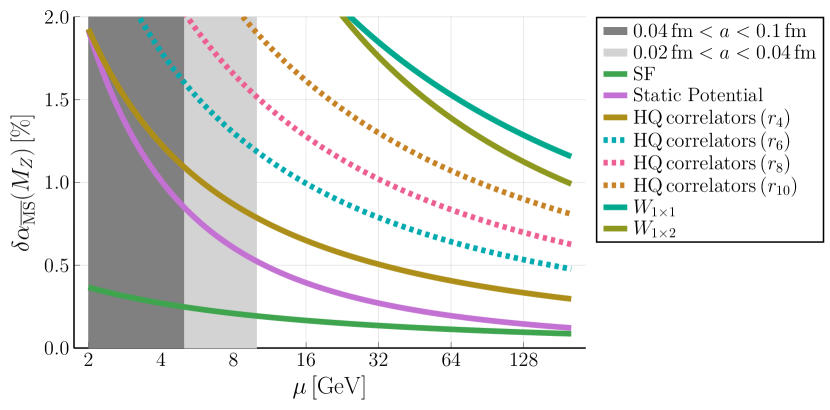
Figure 21: Scale truncation uncertainties for different lattice methods (we quote $\delta_{(2)}$, see section 7.2). The dark shaded region is the current accessible range for large volume lattice simulations nowadays. The light shaded region represents the accessible scales if a reduction by a factor two in the lattice spacing is possible in the future. Note that most methods require a continuum extrapolation with several lattice spacings: in practice the accessible renormalization scales for all methods except finite size scaling (SF) is at least factor two/four smaller than the lattice spacing.

What progress can we expect on this front? Since the window problem is basically a computational limitation we expect to see improvements in the future by just waiting. Computer power has been steadily improving during the last 50 years, and most probably will continue to do so, with exascale machines looming on the horizon. Pushing the UV cutoff of a simulation (i.e. reducing the lattice spacing of the simulation) by a factor two keeping the physical parameters fixed multiplies the computational cost by a factor  $2^{7}=128$. We can therefore expect that on exascale machines the state of the art lattice simulations will be performed on lattice spacing reaching down to $a\approx 0.02$ fm, assuming that topology freezing is still under control on such fine lattices. Beyond the trivial observation that smaller lattice spacing would allow to check the extrapolations thoroughly, the expected increase in computing power would allow the following improvements.

1. Determinations based on QCD vertices and the hadron vacuum polarization, that are nowadays limited by the size of scaling violations, will be able to perform a continuum extrapolation at fixed renormalization scale with several lattice spacing. This will bring the scaling violations under control.

   As of today these methods require to include power corrections as fit parameters to describe the lattice data. Having access to shorter distances would clarify whether the perturbative region can be accessed without having to include these power corrections.

2. Pushing the UV cutoff a factor two higher would allow to match with the perturbative regime at larger renormalization scales.

   For determinations based on the static potential, whose $\beta$-function is known up to 4-loops, one expects truncation errors $\mathcal{O}(\alpha^{3})$ to be reduced. Note however that the latest works have reached high energy scales $Q\approx 5$ GeV. At these high energies the running of the coupling is really slow, and a factor two in scales only reduces the truncation effects in the determination of $\Lambda$ by a factor 2. But more computer power would allow to check the compromises done in the most recent computations thoroughly, and reach solid determinations at the percent level.

   For the determinations based on heavy quark correlators, we also expect a reduction of the perturbative truncation errors by a factor of two. Note that in this case the $\beta$-function is only known to 3-loops (with truncation errors formally $\mathcal{O}(\alpha^{2})$), but the scale typically used in the extractions is significantly lower (we use $Q\approx\bar{m}_{c}$). At these low scales the strong coupling runs faster. Using our estimates for the perturbative truncation effects, these methods could reach a precision $\sim 1\%$ with a solid and conservative estimate of the truncation uncertainties.

   Determinations based on observables defined at the cutoff scale have a more uncertain future. Truncation uncertainties estimated using the scale variation approach point to a not very well behaved perturbative series for these observables. The main benefit would come from the possibility of reaching the perturbative domain without having to add any additional terms to the known perturbative expansion (i.e.  reaching comfortably the perturbative region).

3. Determinations based on finite size scaling are not limited by the systematic error associated with the continuum extrapolation or the truncation of the perturbative series, but by statistics. An increase in computer power by a factor $2^{7}$ would help in reducing the statistical uncertainty dramatically. Naively one expects that the non-perturbative data would become an order of magnitude more precise , decreasing the uncertainty to the level of $0.07\%$.

   This precision clearly is exagerated. Such level of precision would require finer lattices to control the continuum extrapolations. An increase in computer power by $2^{7}$ seems impressive, but this will be eaten by just simulating values of the lattice spacing two times smaller. Some compromise between reducing the statistical errors, and improving the continuum extrapolations would be needed. Moreover some ingredients of the determination (i.e.  the scale setting), that nowadays represent a very small contribution to the total uncertainty, would need to be computed on large volumes where the uncertainties are not merely statistical.

   Nevertheless, it is clear that such an increase in computer power would allow to reduce the uncertainty in $\Lambda$ by a factor two to three. A determination of the strong coupling with an uncertainty $\lesssim 0.3\%$ would in principle be possible. Of course at such level of precision one would have to think about other problems, like electromagnetic contributions to the scale and the running.

Beyond the improvement coming from the increase in computational power, those determinations that are limited by the truncation of the perturbative series could benefit from a better perturbative knowledge. This is especially true for the case of the moments of heavy quark correlators and the observables defined at the cutoff scale, since the relation to the $\overline{\rm MS}$ scheme is only known to 2-loops, and increasing this to 3-loops seems feasible. This would naively suppress the perturbative truncation effects by an extra power of $\alpha$, so potentially a reduction of the error by a factor $3-4$ could be achieved if the size of the perturbative coefficients does not increase. However this assumption is not completely innocent. One should never forget the asymptotic nature of the perturbative series: higher order is never as good as higher renormalization scales.

All in all, experience shows that progress in Lattice QCD comes always from two fronts: computer power, and the new methods and better understanding of the problems by the community. We can speculate the improvements that more computer power would bring, but the most interesting and potentially better improvements coming from the new methods are much more difficult to predict. On this front there is a recent proposal [172] that allows to determine the $N_{\rm f}$-flavor $\Lambda$-parameter from the pure gauge one. The connection between QCD and the pure gauge theory is based on non-perturbatively decoupling hevy quarks (see section 5) using lattice simulations. Since the RG equations are solved in the pure gauge theory (computationally easier), it allows to reach higher energy scales and improve the statistical precision. This idea is discussed in detail in the recent review [41]. This proposal is promosing, but at the time of writing this review there are no results for $\alpha_{s}$ using this method yet.

7.4.1 The pure gauge theory as a perfect laboratory

We have discussed that the limitations usually found in the determination of the strong coupling are not the same as those of other state of the art lattice QCD computations. As a consequence of the window problem, the truncation of the perturbative series and the large scaling violations present in short distance observables represent the limitation of all lattice methods to determine the strong coupling, with the exception of finite size scaling. Statistical accuracy is the main limitation of finite size scaling.

The determination of the $\Lambda$ parameter in the pure gauge theory faces exactly the same limitations. On the other hand, computationally the pure gauge theory is much more tractable than QCD. Simulations algorithms for the pure gauge theory are much more efficient, and smaller physical volumes are acceptable, since finite volume effects are suppressed by the larger mass of the glueballs.

We do not need to wait 10 years to simulate the pure gauge theory at a lattice spacing of $a=0.02$ fm. Testing what precision in the strong coupling could potentially be achieved with 100 times more computer time can be done just by determining the $\Lambda$ parameter in pure gauge.

In fact the situation in pure gauge is not that clear, with some recent determinations claiming an uncertainty $\approx 1.5\%$ in the $\Lambda$ parameter, but disagreeing by about a $5\%$ . A very detailed and precise study is been performed using the static potential [168, 131], but at the moment the preliminary results are inconclusive. There is not a single pure gauge determination using heavy quark correlators.

Given the similarities in the challenges, we hope that the lattice community takes this discrepancy seriously and does not neglect the issue due to the lack of phenomenological interest. Pure gauge studies do not enter in the world average, but in our opinion they will be crucial to help us understand the problems that we have to face and how to solve them.

8 Conclusions

Lattice QCD is, in principle, ideally suited to compute the non-perturbative quantities that are necessary in order to extract the fundamental parameters of the standard model. Being a non-perturbative formulation of QCD, it allows a determination of the value of the strong coupling at energy scales that are measured in units of some well-known QCD spectral quantity (i.e. the proton mass, or the meson decay constants).

Nevertheless there are considerable challenges in obtaining precise values for $\alpha_{s}$. The extraction of the strong coupling requires the application of perturbation theory, and ideally one would like to use perturbation theory at very high energy scales, where good convergence is expected. This wish is in conflict with an intrinsic limitation of any numerical simulation: with finite computing resources only a limited range of scales can be resolved by a single lattice QCD simulation. Datasets that have been generated in order to study the low-energy properties of the strong interactions (i.e.  the spectrum, decay form factors, the anomalous magnetic moment of the muon, …) are limited to reach a few GeV in energy scales at most. This explains why most lattice QCD extractions of $\alpha_{s}$ are limited by the uncertainties associated with the application of perturbation theory and the truncation of the perturbative series at relatively low-energy scales.

In writing this review we have focused on explaining our vision of the field. We have tried to highlight the challenges that lattice determinations of the strong coupling have to face, and insisted on the specific difference between these and other lattice computations.

In the last 15 years lattice QCD has made enormous progress. We have witnessed the surge of dynamical simulations, the values of the lattice spacing has been pushed down to $a\sim 0.05$ fm, some simulations reach physical volumes of 7 fm and simulations at the physical point, that once seemed out of reach, are nowadays common.

This progress has made it possible to produce solid, first principle predictions in the low-energy regime of the strong interactions, with a tremendous impact in flavor physics, searches of beyond the standard model effects and many other topics in high energy physics. It is this very same progress that has pushed the lattice determinations of the strong coupling to the top of the podium: as the overall quality of lattice simulations has improved, the determination of the strong coupling has become dominated by lattice QCD results.

But this situation is changing right now. The limitations in current lattice studies of low-energy hadronic processes are related to the inclusion of charm effects, electromagnetic corrections, and how to deal with the large (power-like) finite volume effects that appear in QED. Solving these issues will have little benefit for the lattice determinations of the strong coupling.

Progress in lattice determinations of $\alpha_{s}$ will come from dedicated approaches. Mere updates of lattice determinations in new ensembles that are generated with the aim of studying electromagnetic corrections, or any other relevant problem of low-energy QCD, will very soon be irrelevant. The lattice community should embrace this as an opportunity to make real progress. The current problems of topology freezing, new techniques to simulate very fine lattices, and more important than anything, the study of alternative techniques to solve multi-scale problems should be taken seriously.

We hope that this review work will further stimulate the lattice community to think about these issues.

The high-luminosity upgrade of the LHC will require high-precision QCD predictions in order to really benefit from the increase in statistics at the experiments. With the dominance of lattice determinations of the strong coupling in the world average, and the relevance of $\alpha_{s}$ for precision phenomelogy at the LHC, it is important for the phenomenology community to understand the problems involved in lattice determinations of the strong coupling, to have some appreciation of the systematic errors that limit these studies, and to foster the progress in the lattice community. Providing a self-contained introduction to the topic for non-lattice specialists has been one of the focal points of our work. We have given an introduction to lattice QCD with an emphasis in the areas that are more relevant in the extractions of the strong coupling: the continuum extrapolation of lattice data, the process of scale setting, and the subtleties involved in the analysis of lattice QCD data at fine lattice spacings. Moreover we have dissected all different approaches to extract $\alpha_{s}$ via lattice simulations, trying to be as critical as possible. With one important exception, lattice extractions of $\alpha_{s}$ based on finite size scaling (see section 6.7), all lattice determinations of the strong coupling represent a compromise between the potentially large cutoff effects present in every lattice determination of a short distance quantity and the potentially large systematic effects associated with the use and truncation of perturbation theory at energy scales of a few GeV. Different lattice methods take different compromises and suffer from these effects in very different ways. Our point of view is that only methods that show convincing evidence to have reached the perturbative running and are able to explore the continuum limit with several lattice spacing should be used to determine the fundamental parameters of the standard model. We have studied the perturbative truncation effects of the most reliable approaches in detail, trying to provide a broad picture of each of the methods. Our conclusions are that there are at least three methods that, as of today, allow a reliable extraction of the strong coupling: finite size scaling (section 6.7), the static potential (section 6.2) and moments of heavy quark correlators (section 6.3), although with very different degrees of reliance. The precision of these extractions, as well as the potential to improve substantially the current determinations, have been analyzed.

On the other hand we have not tried to evaluate each publication. The interested reader in this fine detailed perspective should consult the excellent work of the FLAG review.

Let us end this review with a comment on the status of the world average. The most precise lattice determinations show a good agreement. The world average value of the strong coupling performed by the PDG [100] includes all phenomenological and lattice computations. In the PDG average individual works are classified according the method of extraction, and pre-averaged, before determining the final world average. The list of methods includes several phenomenological procedure (DIS, $\tau$ decays, $e^{+}-e^{-}$, …). The rationale behind such a procedure is that different works within the same pre-average have to face the same systematic effects. As we have seen different lattice strategies for the extraction of the strong coupling are limited by very different reasons. In fact, once the continuum extrapolations are under control, lattice QCD and phenomenological determinations stand on the same footing, and have to face very similar challenges (see also [32]). Many lattice QCD extractions using moments of heavy quark correlators are somehow similar to extractions using $\tau$ decays: the extraction is performed at a relatively low scale and the systematics associated with the use of perturbation theory at such low scales dominate the error budget. Lattice QCD extractions of the strong coupling based on finite size scaling are similar to phenomenological extractions based on $Z$ boson decays in the sense that they are performed directly at the electroweak scale and limited by statistics.

We would like to see a world average of $\alpha_{s}$ that groups different extractions based on similar systematics. Questions like at What scale is perturbation theory applied?, What range of scales show agreement with the perturbative running?, What are the scale variation effects in the extractions? are the key questions to asses the quality of any determination of $\alpha_{s}$, regardless of it being a lattice or a phenomenology extraction. We hope that this work is also useful to the brave that attempt to produce such a world average.

Appendix A Challenges in Lattice QCD

A.1 Topology freezing and large autocorrelation times

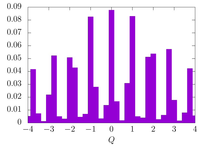
(a) $32^{4}$ with $a=0.08$ fm.

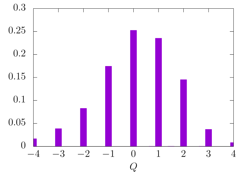
(b) $48^{4}$ with $a=0.03$ fm.

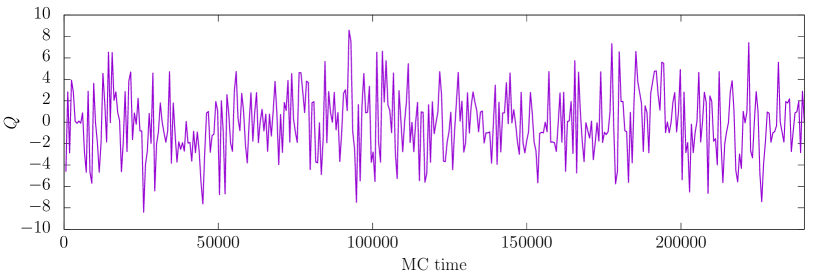
(c) $32^{4}$ with $a=0.08$ fm.

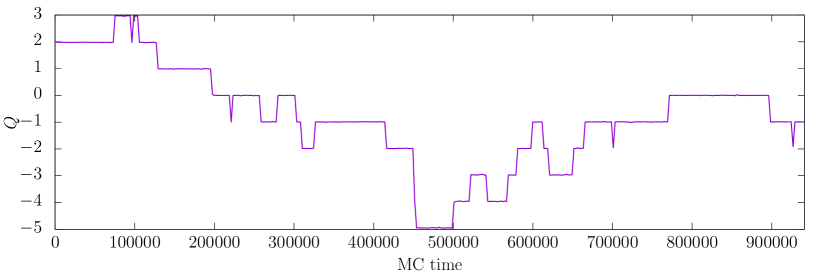
(d) $48^{4}$ with $a=0.03$ fm.

Figure 22: The topological charge is not quantized on the lattice (here we use the definition based on the Gradient flow), but in practice values for $Q$ in simulations with very fine lattice spacing cluster very close to integer values. At the same time the transition between different topological sectors becomes less and less frequent in simulation time.

Most definitions of the topological charge are not quantized on the lattice. It is only when the lattice spacing of a simulation is small enough ($a<0.05$ fm), that the values of the topological charge measured on the lattice cluster close to integer values. The different topological sectors emerge as the simulation approaches the continuum limit. As was first realized in [87], at the same time the transition between different topological sectors also becomes less and less frequent at small lattice spacings (see fig. 22).

This has implications for the error estimation of observables that couple strongly with the topological charge. Lattice measurements of these observables are correlated for very long simulation times, since they feel the topological sector in which they have been measured. Getting a solid estimate of the statistical error of such observables is really difficult since the topological charge is not well sampled.

The most clean solutions to the problem improve the sampling of different topological sectors by changing the boundary conditions of the lattice simulation in Euclidean time [176, 160]. In these cases the topological charge is no longer quantized (even in the continuum), and can fluctuate. In other cases the problem can be bypassed. One can perform the simulations at fixed topological sector and deal with power law finite volume effects if necessary [177]. Recently simulations on very large physical volumes so that the finite volume effects of a fixed topology become irrelevant have been performed in the pure gauge theory[85].

All in all it is pretty uncomfortable that no algorithm is able to sample correctly the theory at fine lattice spacings. It remains an algorithmic challenge to find an efficient algorithm for the simulation of QCD at fine lattice spacings. In the meantime, the accuracy of the statistical errors quoted for simulations at fine lattice spacings without the use of some variant of open boundary conditions has to be taken with a grain of salt.

A.2 Signal to noise problem

Figure 23: The variance of a meson at large Euclidean times is dominated by two mesons propagating. On the other hand the variance of a nucleon two-point functions at large Euclidean times is not dominated by the propagation of two baryons, but by the propagation of three meson states.

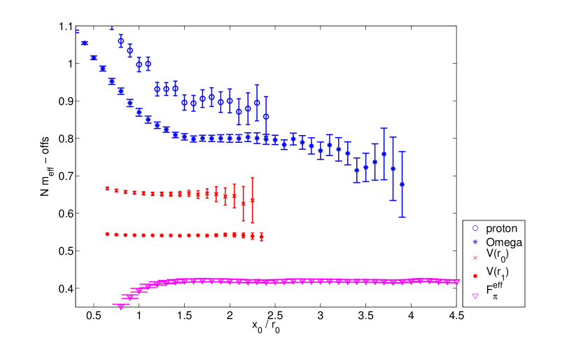
Figure 24: Several meson and baryon correlators, as well as the static potential at different distances (shifted vertically). Meson correlators, do not have a signal to noise problem, and its value can be determined with high precision at large Euclidean times. (Source: $m_{p}$ [178], $m_{\Omega}$ [179], $V(\approx r_{0}),V(\approx r_{1})$ [180], $f_{\pi}$ [181]).

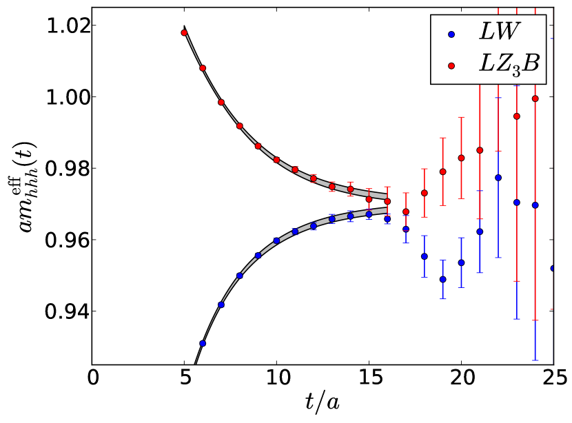
Figure 25: Precise values of baryon masses require to fit the correlators at small Euclidean times, where there are significant contributions from excited states. (Source [182])

Every observable ($O$) in lattice QCD is computed as an avegare over configurations generated by Monte Carlo sampling

$$\langle O\rangle=\frac{1}{N}\sum_{t=1}^{N}O[U_{t}]+\mathcal{O}({1}/{\sqrt{N}})\,.$$ (230)

Here $U_{t}$ represents the configuration at Monte Carlo time $t$ and $O[U_{t}]$ is the value of the observable measured on such a configuration. All observables carry an statistical uncertainty $\mathcal{O}({1}/{\sqrt{N}})$ due to this stochastic estimation. The error in the observable is proportional to the variance

$$(\delta O)^{2}\propto\langle O^{2}\rangle-\langle O\rangle^{2}\,.$$ (231)

The signal to noise problem refers to the particular behavior of the error in some correlators. If we examine the case of a meson correlator, like the pion, we have

$$\langle[\bar{u}\gamma_{5}d(x)\,\bar{d}\gamma_{5}u(0)]\rangle^{2} \stackrel{{\scriptstyle\small{x_{0}\to\infty}}}{{\sim}} Ae^{-2M_{\pi}x_{0}}+\dots$$ (232)

$$\langle[\bar{u}\gamma_{5}d(x)\,\bar{d}\gamma_{5}u(0)]^{2}\rangle \stackrel{{\scriptstyle\small{x_{0}\to\infty}}}{{\sim}} A^{\prime}e^{-2M_{\pi}x_{0}}+\dots$$ (233)

The first equation is clear, since this is just the squared $\pi$ propagator. The second equation becomes clear when one realizes that the Wick contractions in the expectation value $\langle O^{2}\rangle$ can be understood as 2 $\pi$ mesons propagating between Euclidean times $0$ and $x_{0}$ (see fig. 23). On the other hand for the case of a baryon, like the proton $p$, the correlators have the form ($a,b,c$ are color indices and $C$ the charge conjugation matrix)

$$\langle u^{T}_{a}C\gamma_{5}u_{b}d_{c}\epsilon^{abc}(x)\,[u^{T}_{a}C\gamma_{5}u_{b}d_{c}\epsilon^{abc}(0)]^{\dagger}\rangle^{2} \stackrel{{\scriptstyle\small{x_{0}\to\infty}}}{{\sim}} Ae^{-2M_{p}x_{0}}+\dots$$ (234)

$$\langle\left\{u^{T}_{a}C\gamma_{5}u_{b}d_{c}\epsilon^{abc}(x)\,[u^{T}_{a}C\gamma_{5}u_{b}d_{c}\epsilon^{abc}(0)]^{\dagger}\right\}^{2}\rangle \stackrel{{\scriptstyle\small{x_{0}\to\infty}}}{{\sim}} A^{\prime}e^{-3M_{\pi}x_{0}}+\dots$$ (235)

In this case the dominant contribution at large Euclidean times for the expectation value $\langle O^{2}\rangle$ comes from three $\pi$ meson propagating between Euclidean times 0 and $x_{0}$ (fig. 23). The term with two protons propagating also contributes to this expectation value, but with a term $\propto e^{-2M_{p}x_{0}}$ that decays much faster. See also [183] for more details.

In summary the ratio signal-to-noise shows a quite different behavior in both cases (see fig. 23)

$$\frac{C_{\pi}(x_{0})}{\delta C_{\pi}(x_{0})} \stackrel{{\scriptstyle\small{x_{0}\to\infty}}}{{\sim}} 1\,,$$ (236)

$$\frac{C_{p}(x_{0})}{\delta C_{p}(x_{0})} \stackrel{{\scriptstyle\small{x_{0}\to\infty}}}{{\sim}} e^{\left(M_{p}-\frac{3}{2}M_{\pi}\right)x_{0}}\,.$$ (237)

This exponential increase in the signal to noise has in practice important implications: it is almost impossible to determine the value of a baryon correlator with high precision at distances of 1 fm and larger. Precise determinations of baryon masses extract such quantities from the values of the correlator at relatively small Euclidean times, where there is significant contamination of excited estates. The use of different interpolating operators (with different excited state contamination) and the use of several numerical techniques are common to deal with this situation (see figs. 24 and 25).

Once more, the situation is far from ideal. Such basic quantities as baryon masses ideally should be determined without dealing with complicated systematic effects in the determination of the effective mass plateau, but currently there no known techniques that allow the precise extraction of baryon masses at distances $\sim 1$ fm.

Appendix B Scale variation estimation of truncation errors

The definition of a non perturbative coupling in lattice QCD uses an observable $O(\mu)$ that depends on only one scale ($\mu$) and can be determined non perturbatively. This observable has a perturbative expansion when $\mu\gg\Lambda$, that after a proper normalization can be written as

$$O(\mu)\raisebox{-0.43057pt}{ $\stackrel{{\scriptstyle\small{\mu\to\infty}}}{{\sim}}$}\alpha_{\overline{\rm MS}}(\mu)+\sum_{k>1}c_{k}\alpha_{\overline{\rm MS}}^{k}(\mu)\,.$$ (239)

The RG evolution of $\alpha_{\overline{\rm MS}}(\mu)$ is given by the $\beta$ function, and can be used to obtain an estimate the truncation effects of the perturbative series, which is valid under certain assumptions on the size of the unknown coefficients. The truncated series

$$O^{(n)}(\mu)=\alpha_{\overline{\rm MS}}(\mu)+\sum_{k=2}^{n}c_{k}\alpha_{\overline{\rm MS}}^{k}(\mu)+\mathcal{O}(\alpha_{\overline{\rm MS}}^{n+1})\,,$$ (240)

can be rewritten, with the same level of precision, as

$$O^{(n)}(\mu,s)=\alpha_{\overline{\rm MS}}(\mu^{\prime})+\sum_{k=2}^{n}c_{k}^{\prime}(s)\alpha_{\overline{\rm MS}}^{k}(\mu^{\prime})+\mathcal{O}(\alpha_{\overline{\rm MS}}^{n+1})\,,\qquad(s=\mu^{\prime}/\mu)\,.$$ (241)

Note that the dependence of $O^{(n)}(\mu,s)$ on $s$ is only due to the truncation of the perturbative series. The coefficients

$$c_{k}^{\prime}(s)=\sum_{l=0}^{k-1}c^{\prime}_{k,l}\log^{l}(s)\,,$$ (242)

can all be determined from $c_{k}$ that appear in Eq. (240) thanks to the recursion

$$c^{\prime}_{k,0} = c_{k}\,,$$ (243)

$$c^{\prime}_{k,l} = \frac{2}{l}\sum_{j=0}^{k-1}j(4\pi)^{k-j}b_{k-j-1}c_{j,l-1}^{\prime}\,,$$ (244)

where $b_{n}$ are the coefficients of the $\beta$ function Eq. (9).

Given a value for the observable $O_{\rm ref}=O(\mu_{\rm ref})$ determined on the lattice at some value of the scale $\mu_{\rm ref}$, we can compare the determination of $\alpha_{\overline{\rm MS}}(M_{Z})$ coming from using Eq. (241) for different values of $s$, and use them as an estimate of the truncation uncertainties. Note that usually lattice works with $N_{\rm f}=2+1$ or $N_{\rm f}=2+1+1$ QCD, which means that in order to obtain $\alpha_{\overline{\rm MS}}(M_{Z})$ one needs to match the couplings through the bottom and/or charm thresholds.

For numerical results the reader should look at the RunDec package [184, 101]. We also provide a freely available software ScaleErrors to determine the truncation uncertainties in $\alpha_{s}$ as we detail below.

B.1 The case of the Schrödinger Funcional coupling in full detail

In this section we describe in full detail our procedure for estimating the impact of scale variations in the case of works based on finite size scaling. The implementation for the other observables is sketched briefly in the rest of the appendix.

Our starting point is the value of the three flavor theory, that we assume to be

$$\Lambda^{(3)}_{\overline{\rm MS}}=341\,{\rm MeV}\,,$$ (245)

and the perturbative expansion of the Schrödinger Functional (SF) coupling, that is measured on a finite volume at the scale $\mu=1/L$. For $N_{\rm f}=3$ QCD we have

$$\alpha_{\rm SF}(\mu) = \alpha_{\overline{\rm MS}}(s\mu)-[1.37520970-1.43239449\log(s)]\alpha_{\overline{\rm MS}}^{2}(s\mu)$$

$$+ [0.57120172-3.12911612\log(s)+2.05175397\log(s)^{2}]\alpha_{\overline{\rm MS}}^{3}(s\mu)\,.$$

where the $\log$ terms can be computed from expression (241) and the perturbative computation [185, 186]. We point that the routine scale_errors from the package ScaleErrors.jl (see footnote 39), takes as input the perturbative coefficients

$$c_{k}(1)=\{1.0,-1.3752097,0.571202\}\,,$$ (247)

and determines the truncation uncertainties exactly as described below.

We proceed as follows:

1. Chose a reference value for the scale $s_{\rm ref}$ and solve the non linear equation

   $$\frac{\Lambda^{(3)}_{\overline{\rm MS}}}{s_{\rm ref}\mu}=\left[b_{0}\bar{g}^{2}(s_{\rm ref}\mu)\right]^{-\frac{b_{1}}{2b_{0}^{2}}}\,e^{-\frac{1}{2b_{0}\bar{g}^{2}(s_{\rm ref}\mu)}}\,\exp\left\{-\int_{0}^{\bar{g}(s_{\rm ref}\mu)}{\rm d}x\,\left[\frac{1}{\beta_{\overline{\rm MS}}(x)}+\frac{1}{b_{0}x^{3}}-\frac{b_{1}}{b_{0}^{2}x}\right]\right\}\,.$$ (248)

   in order to obtain $\alpha_{\overline{\rm MS}}(s_{\rm ref}\mu)\equiv\bar{g}^{2}(s_{\rm ref}\mu)/(4\pi)$. For example, using $\mu=80$ GeV, $s_{\rm ref}=2$ and the 5-loop $\beta_{\overline{\rm MS}}$ function together with our reference value of $\Lambda^{(3)}_{\overline{\rm MS}}=341$ MeV we get

   $$\alpha_{\overline{\rm MS}}(s_{\rm ref}\mu)=0.09703895\,.$$ (249)

2. This value is plugged in Eq. (B.1) in order to obtain

   $$\alpha_{\rm SF}(80\,{\rm GeV})=0.09287934\,.$$ (250)

3. We can now solve the polynomial equation (B.1) for different values of $s$ and the l.h.s fixed to the value in Eq. (250). i.e.  Using $s=4$ ($s\mu=320$ GeV), we solve

   $$0.09287934 = \alpha_{\overline{\rm MS}}(s\mu)-[1.37520970-1.43239449\log(s)]\alpha_{\overline{\rm MS}}^{2}(s\mu)$$

   $$+ [0.57120172-3.12911612\log(s)+2.05175397\log(s)^{2}]\alpha_{\overline{\rm MS}}^{3}(s\mu)\,,$$

   To obtain

   $$\alpha_{\overline{\rm MS}}(320\,{\rm GeV})=0.08802818\,.$$ (252)

4. The two values of the coupling Eqs. (249), (252) should be equivalent, except for the truncation uncertainties. In order to compare them, we run the two values to a common scale ($M_{Z}$), crossing the charm and bottom thresholds. We get

   $$\alpha_{\overline{\rm MS}}(80\,{\rm GeV})=0.09703895 \Longrightarrow \alpha^{(N_{\rm f}=5)}_{\overline{\rm MS}}(M_{Z})=0.11851821\,,$$ (253a)

   $$\alpha_{\overline{\rm MS}}(320\,{\rm GeV})=0.08802818 \Longrightarrow \alpha^{(N_{\rm f}=5)}_{\overline{\rm MS}}(M_{Z})=0.11843281\,.$$ (253b)

   Let us give a few details on how this is done. Using the 5-loop three flavor beta function and the charm quark mass $m_{\rm c}^{\star}=m_{\rm c}(m_{\rm c})=1275.0$ MeV, we solve the non-linear equation

   $$\log\left(\frac{80\,{\rm GeV}}{m_{\rm c}^{\star}}\right)=\int_{\bar{g}(m_{\rm c})}^{\bar{g}(80\,{\rm GeV})}\frac{{\rm d}x}{\beta_{\overline{\rm MS}}^{(N_{\rm f}=3)}(x)}\,.$$ (254)

   in order to obtain the value of the three flavor coupling at the charm scale. We obtain

   $$\alpha_{\overline{\rm MS}}(80\,{\rm GeV})=0.09703895\Longrightarrow\alpha_{\overline{\rm MS}}(m_{\rm c}^{\star})=0.39566020\,.$$ (255)

   We now “cross the charm threshold” by using the decoupling relations [17, 18, 19, 20, 21] to determine the four flavor coupling at the scale $m_{\rm c}^{\star}$.

   $$\alpha_{\overline{\rm MS}}(m_{\rm c}^{\star})=0.39566020\Longrightarrow\alpha_{\overline{\rm MS}}^{(N_{\rm f}=4)}(m_{\rm c}^{\star})=0.393947409\,.$$ (256)

   A similar procedure is used to run the coupling to the bottom quark threshold $m_{\rm b}^{\star}=m_{\rm b}(m_{\rm b})=4198.0$ MeV, and convert to the five flavor coupling

   $$\alpha_{\overline{\rm MS}}^{(N_{\rm f}=4)}(m_{\rm c}^{\star})=0.393947409\Longrightarrow\alpha_{\overline{\rm MS}}^{(N_{\rm f}=4)}(m_{\rm b}^{\star})=0.226549731\Longrightarrow\alpha_{\overline{\rm MS}}^{(N_{\rm f}=5)}(m_{\rm b}^{\star})=0.226311579\,.$$

   Finally, one uses Eq. (254) using the five flavor $\beta_{\overline{\rm MS}}$ function to run the coupling to the scale $M_{Z}$.

5. Finally, the difference between values of $\alpha_{\overline{\rm MS}}^{(N_{\rm f}=5)}(M_{Z})$ in Eqs. (253)

   $$\delta\alpha_{\overline{\rm MS}}^{(N_{\rm f}=5)}(M_{Z})=8.5\times 10^{-5}\qquad[0.07\%]\,.$$ (257)

   can be used as an estimate of the truncation uncertainties.

B.2 The static potential

We start from the perturbative expression of the potential $V(r)$

$$V(r)=-\frac{4}{3r}\sum_{n=0}P_{n}\left(\frac{\alpha_{s}}{4\pi}\right)^{n}\,,$$ (258)

where $\alpha_{s}=\alpha_{\overline{\rm MS}}(1/r)$ is the strong coupling. Note that we ignore the logarithmic corrections $\propto\log\alpha$ due to the IR divergent nature of $V(r)$. See section 6.2 for more details. Using the RG equations, we have

$$\frac{{\rm d}\alpha_{s}}{{\rm d}r}=\frac{2\alpha_{s}^{2}}{r}\sum_{i=0}(4\pi)^{i}b_{i}\alpha_{s}^{i}\,,$$ (259)

which we can use to evaluate the derivative of the static potential with respect to the scale $r$:

$$F(r)=\frac{{\rm d}V(r)}{{\rm d}r}=\frac{4}{3r^{2}}\sum_{n=0}\frac{P_{n}}{(4\pi)^{n}}\alpha_{s}^{n+1}-\frac{4}{3r^{2}}\sum_{n=0}\frac{2(n+1)P_{n}}{(4\pi)^{n}}\alpha_{s}^{n+2}\left[\sum_{j=0}(4\pi)^{j+1}b_{j}\alpha_{s}^{j}\right]\,.$$ (260)

Collecting the coefficients in the equation above, we get an expression for the perturbative expansion of the force, as a function of the number of flavors $N_{f}$. We use the force as the observable that determines the strong coupling constant, with the typical scale associated to the observable being $\mu=1/r$. In $N_{\rm f}=3$ QCD the known terms in the perturbative series [120, 187, 125, 188] together with expression Eq. (241) allows to write

$$\begin{split}\alpha_{\rm qq}(\mu)\raisebox{-0.43057pt}{ $\stackrel{{\scriptstyle\small{\mu\to\infty}}}{{\sim}}$}&\alpha_{\overline{\rm MS}}(s\mu)+[-0.0485502+1.43239449\log(s)]\alpha^{2}_{\overline{\rm MS}}(s\mu)\\ +\,&[0.687447+0.67148339\log(s)+2.05175397\log(s)^{2}]\alpha^{3}_{\overline{\rm MS}}(s\mu)\\ +\,&[0.818808+3.52427341\log(s)+2.6037989\log(s)^{2}+2.93892108\log(s)^{3}]\alpha^{4}_{\overline{\rm MS}}(s\mu)\\ +\,&\dots\,.\end{split}$$ (261)

The scale of fastest apparent convergence is reached at $s^{\star}=1.034475$, and the maximum scale reached in current state of the art determinations is 8 GeV, albeit at a single value of the lattice spacing.

IR divergences affect the term $\propto\alpha_{\overline{\rm MS}}^{4}(Q)$. If we assume a fixed value for the ultra-soft scale $\nu_{\rm us}=2$ GeV, the last term would read instead:

$$\dots+\alpha^{4}_{\overline{\rm MS}}(sQ)[0.246933+3.52427341\log(s)+2.6037989\log(s)^{2}+2.93892108\log(s)^{3}]\,.$$ (262)

This has an effect in the truncation uncertainties at the $20\%$ level.

B.3 HQ correlators

The perturbative expansions for the ratios of moments $\alpha_{\rm HQ,n}$ is given by[136, 189, 190]:

$$\alpha_{\rm HQ,4}(\mu) \stackrel{{\scriptstyle\small{\mu\to\infty}}}{{\sim}} \alpha_{\overline{\rm MS}}(s\mu)-[0.07762325-1.43239449\log(s)]\alpha_{\overline{\rm MS}}^{2}(s\mu)$$

$$+ [0.07957445+.58819524\log(s)+2.05175397\log(s)^{2}]\alpha_{\overline{\rm MS}}^{3}(s\mu)+\dots\,.$$

$$\alpha_{\rm HQ,6}(\mu) \stackrel{{\scriptstyle\small{\mu\to\infty}}}{{\sim}} \alpha_{\overline{\rm MS}}(s\mu)+[0.77386542+1.43239449\log(s)]\alpha_{\overline{\rm MS}}^{2}(s\mu)$$

$$- [0.08560363-3.02753059\log(s)-2.05175397\log(s)^{2}]\alpha_{\overline{\rm MS}}^{3}(s\mu)+\dots\,.$$

$$\alpha_{\rm HQ,8}(\mu) \stackrel{{\scriptstyle\small{\mu\to\infty}}}{{\sim}} \alpha_{\overline{\rm MS}}(s\mu)+[1.08917060+1.43239449\log(s)]\alpha_{\overline{\rm MS}}^{2}(s\mu)$$

$$+ [0.20034888+3.93081340\log(s)+2.05175397\log(s)^{2}]\alpha_{\overline{\rm MS}}^{3}(s\mu)+\dots\,.$$

$$\alpha_{\rm HQ,10}(\mu) \stackrel{{\scriptstyle\small{\mu\to\infty}}}{{\sim}} \alpha_{\overline{\rm MS}}(s\mu)+[1.44848150+1.43239449\log(s)]\alpha_{\overline{\rm MS}}^{2}(s\mu)$$

$$+ [0.66519861+4.96016330\log(s)+2.05175397\log(s)^{2}]\alpha_{\overline{\rm MS}}^{3}(s\mu)+\dots\,.$$

B.4 Wilson loops

For the couplings defined in Eqs (226), defined from Wilson loops, the perturbative expansion reads [170]:

$$\alpha_{\rm W_{11}}(\mu) \stackrel{{\scriptstyle\small{\mu\to\infty}}}{{\sim}} \alpha_{\overline{\rm MS}}(s\mu)-[0.87811924-1.43239449\log(s)]\alpha_{\overline{\rm MS}}^{2}(s\mu)$$

$$+ [4.20161085-1.70505684\log(s)+2.05175397\log(s)^{2}]\alpha_{\overline{\rm MS}}^{3}(s\mu)+\dots\,.$$

$$\alpha_{\rm W_{12}}(\mu) \stackrel{{\scriptstyle\small{\mu\to\infty}}}{{\sim}} \alpha_{\overline{\rm MS}}(s\mu)+[0.79128076+1.43239449\log(s)]\alpha_{\overline{\rm MS}}^{2}(s\mu)$$

$$+ [3.18658638+3.07742188\log(s)+2.05175397\log(s)^{2}]\alpha_{\overline{\rm MS}}^{3}(s\mu)+\dots\,.$$

The scale of fastest apparent convergence is reached at $s^{\star}=1.4252357$, and the maximum scale reached in current state of the art determinations is $4.4$ GeV.

References

- [1] Flavour Lattice Averaging Group Collaboration, S. Aoki et al., “FLAG Review 2019,” arXiv:1902.08191 [hep-lat].
- [2] R. H. Parker, C. Yu, W. Zhong, B. Estey, and H. Müller, “Measurement of the fine-structure constant as a test of the Standard Model,” Science 360 (2018) 191, arXiv:1812.04130 [physics.atom-ph].
- [3] D. Hanneke, S. Fogwell, and G. Gabrielse, “New Measurement of the Electron Magnetic Moment and the Fine Structure Constant,” Phys. Rev. Lett. 100 (2008) 120801, arXiv:0801.1134 [physics.atom-ph].
- [4] H. D. Politzer, “Reliable Perturbative Results for Strong Interactions?,” Phys. Rev. Lett. 30 (1973) 1346–1349. [,274(1973)].
- [5] D. J. Gross and F. Wilczek, “Ultraviolet Behavior of Nonabelian Gauge Theories,” Phys. Rev. Lett. 30 (1973) 1343–1346. [,271(1973)].
- [6] J. Callan, Curtis G., “Broken scale invariance in scalar field theory,” Phys. Rev. D 2 (1970) 1541–1547.
- [7] K. Symanzik, “Small distance behavior in field theory and power counting,” Commun. Math. Phys. 18 (1970) 227–246.
- [8] W. A. Bardeen, A. J. Buras, D. W. Duke, and T. Muta, “Deep Inelastic Scattering Beyond the Leading Order in Asymptotically Free Gauge Theories,” Phys. Rev. D18 (1978) 3998.
- [9] P. Boyle, L. Del Debbio, and A. Khamseh, “Massive momentum-subtraction scheme,” Phys. Rev. D95 no. 5, (2017) 054505, arXiv:1611.06908 [hep-lat].
- [10] ALPHA Collaboration, P. Fritzsch, R. Sommer, F. Stollenwerk, and U. Wolff, “Symanzik Improvement with Dynamical Charm: A 3+1 Scheme for Wilson Quarks,” JHEP 06 (2018) 025, arXiv:1805.01661 [hep-lat].
- [11] T. van Ritbergen, J. A. M. Vermaseren, and S. A. Larin, “The Four loop beta function in quantum chromodynamics,” Phys. Lett. B400 (1997) 379–384, arXiv:hep-ph/9701390 [hep-ph].
- [12] M. Czakon, “The Four-loop QCD beta-function and anomalous dimensions,” Nucl. Phys. B710 (2005) 485–498, arXiv:hep-ph/0411261 [hep-ph].
- [13] P. A. Baikov, K. G. Chetyrkin, and J. H. Kḧn, “Five-Loop Running of the QCD coupling constant,” Phys. Rev. Lett. 118 no. 8, (2017) 082002, arXiv:1606.08659 [hep-ph].
- [14] T. Luthe, A. Maier, P. Marquard, and Y. Schröder, “Towards the five-loop Beta function for a general gauge group,” JHEP 07 (2016) 127, arXiv:1606.08662 [hep-ph].
- [15] F. Herzog, B. Ruijl, T. Ueda, J. A. M. Vermaseren, and A. Vogt, “The five-loop beta function of Yang-Mills theory with fermions,” JHEP 02 (2017) 090, arXiv:1701.01404 [hep-ph].
- [16] A. Hasenfratz and P. Hasenfratz, “The Connection Between the Lambda Parameters of Lattice and Continuum QCD,” Phys. Lett. 93B (1980) 165. [,241(1980)].
- [17] K. G. Chetyrkin, J. H. Kuhn, and C. Sturm, “QCD decoupling at four loops,” Nucl. Phys. B744 (2006) 121–135, arXiv:hep-ph/0512060 [hep-ph].
- [18] S. Weinberg, “Effective Gauge Theories,” Phys. Lett. B91 (1980) 51–55.
- [19] W. Bernreuther and W. Wetzel, “Decoupling of Heavy Quarks in the Minimal Subtraction Scheme,” Nucl. Phys. B197 (1982) 228–236. [Erratum: Nucl. Phys.B513,758(1998)].
- [20] A. G. Grozin, M. Hoeschele, J. Hoff, M. Steinhauser, M. Hoschele, J. Hoff, and M. Steinhauser, “Simultaneous decoupling of bottom and charm quarks,” JHEP 09 (2011) 066, arXiv:1107.5970 [hep-ph].
- [21] Y. Schroder and M. Steinhauser, “Four-loop decoupling relations for the strong coupling,” JHEP 01 (2006) 051, arXiv:hep-ph/0512058 [hep-ph].
- [22] A. Athenodorou, J. Finkenrath, F. Knechtli, T. Korzec, B. Leder, M. K. Marinkovic, and R. Sommer, “How perturbative are heavy sea quarks?,” arXiv:1809.03383 [hep-lat].
- [23] T. Korzec, F. Knechtli, S. Cali, B. Leder, and G. Moir, “Impact of dynamical charm quarks,” PoS LATTICE2016 (2017) 126, arXiv:1612.07634 [hep-lat].
- [24] Particle Data Group Collaboration, P. Zyla et al., “Review of Particle Physics,” to be published in Prog. Theor. Exp. Phys. 2020 083C01 (2020) .
- [25] A. Pich, “Precision Tau Physics,” Prog. Part. Nucl. Phys. 75 (2014) 41–85, arXiv:1310.7922 [hep-ph].
- [26] P. A. Baikov, K. G. Chetyrkin, and J. H. Kuhn, “Order alpha**4(s) QCD Corrections to Z and tau Decays,” Phys. Rev. Lett. 101 (2008) 012002, arXiv:0801.1821 [hep-ph].
- [27] P. A. Baikov, K. G. Chetyrkin, J. H. Kuhn, and J. Rittinger, “Complete QCD Corrections to Hadronic -Decays,” Phys. Rev. Lett. 108 (2012) 222003, arXiv:1201.5804 [hep-ph].
- [28] P. A. Baikov, K. G. Chetyrkin, J. H. Kuhn, and J. Rittinger, “Adler Function, Sum Rules and Crewther Relation of Order O(): the Singlet Case,” Phys. Lett. B714 (2012) 62–65, arXiv:1206.1288 [hep-ph].
- [29] R. D. Ball, V. Bertone, L. Del Debbio, S. Forte, A. Guffanti, J. I. Latorre, S. Lionetti, J. Rojo, and M. Ubiali, “Precision NNLO determination of using an unbiased global parton set,” Phys. Lett. B707 (2012) 66–71, arXiv:1110.2483 [hep-ph].
- [30] NNPDF Collaboration, R. D. Ball, S. Carrazza, L. Del Debbio, S. Forte, Z. Kassabov, J. Rojo, E. Slade, and M. Ubiali, “Precision determination of the strong coupling constant within a global PDF analysis,” Eur. Phys. J. C78 no. 5, (2018) 408, arXiv:1802.03398 [hep-ph].
- [31] L. A. Harland-Lang, A. D. Martin, P. Motylinski, and R. S. Thorne, “Uncertainties on in the MMHT2014 global PDF analysis and implications for SM predictions,” Eur. Phys. J. C75 no. 9, (2015) 435, arXiv:1506.05682 [hep-ph].
- [32] G. P. Salam, “The strong coupling: a theoretical perspective,” in From My Vast Repertoire …: Guido Altarelli’s Legacy, A. Levy, S. Forte, and G. Ridolfi, eds., pp. 101–121. 2019. arXiv:1712.05165 [hep-ph].
- [33] S. Forte and Z. Kassabov, “Why Cannot be Determined from Hadronic Processes without Simultaneously Determining the Parton Distributions,” arXiv:2001.04986 [hep-ph].
- [34] ALPHA Collaboration, M. Dalla Brida, P. Fritzsch, T. Korzec, A. Ramos, S. Sint, and R. Sommer, “Determination of the QCD -parameter and the accuracy of perturbation theory at high energies,” Phys. Rev. Lett. 117 no. 18, (2016) 182001, arXiv:1604.06193 [hep-ph].
- [35] ALPHA Collaboration, M. Dalla Brida, P. Fritzsch, T. Korzec, A. Ramos, S. Sint, and R. Sommer, “A non-perturbative exploration of the high energy regime in QCD,” Eur. Phys. J. C78 no. 5, (2018) 372, arXiv:1803.10230 [hep-lat].
- [36] M. Cacciari and N. Houdeau, “Meaningful characterisation of perturbative theoretical uncertainties,” JHEP 09 (2011) 039, arXiv:1105.5152 [hep-ph].
- [37] NNPDF Collaboration, R. Abdul Khalek et al., “A First Determination of Parton Distributions with Theoretical Uncertainties,” arXiv:1905.04311 [hep-ph].
- [38] NNPDF Collaboration, R. Abdul Khalek et al., “Parton Distributions with Theory Uncertainties: General Formalism and First Phenomenological Studies,” Eur. Phys. J. C 79 no. 11, (2019) 931, arXiv:1906.10698 [hep-ph].
- [39] M. Beneke, “Renormalons,” Phys. Rept. 317 (1999) 1–142, arXiv:hep-ph/9807443 [hep-ph].
- [40] G. ’t Hooft, “Can We Make Sense Out of Quantum Chromodynamics?,” Subnucl. Ser. 15 (1979) 943.
- [41] M. Dalla Brida, “Past, present, and future of precision determinations of the QCD parameters from lattice QCD,” in 38th International Symposium on Lattice Field Theory. 12, 2020. arXiv:2012.01232 [hep-lat].
- [42] W. Bietenholz, U. Gerber, M. Pepe, and U. J. Wiese, “Topological Lattice Actions,” JHEP 12 (2010) 020, arXiv:1009.2146 [hep-lat].
- [43] K. G. Wilson, “Confinement of quarks,” Phys. Rev. D 10 no. 8, (Oct., 1974) 2445–2459.
- [44] H. B. Nielsen and M. Ninomiya, “No Go Theorem for Regularizing Chiral Fermions,” Phys. Lett. 105B (1981) 219–223.
- [45] L. H. Karsten, “Lattice Fermions in Euclidean Space-time,” Phys. Lett. B 104 (1981) 315–319.
- [46] A. Pelissetto, “LATTICE NONLOCAL CHIRAL FERMIONS,” Annals Phys. 182 (1988) 177.
- [47] K. G. Wilson, “Quarks and Strings on a Lattice,” in New Phenomena in Subnuclear Physics: Proceedings, International School of Subnuclear Physics, Erice, Sicily, Jul 11-Aug 1 1975. Part A, p. 99. 1975. [,0069(1975)].
- [48] B. Sheikholeslami and R. Wohlert, “Improved Continuum Limit Lattice Action for QCD with Wilson Fermions,” Nucl. Phys. B259 (1985) 572.
- [49] M. Lüscher, S. Sint, R. Sommer, and P. Weisz, “Chiral symmetry and O(a) improvement in lattice QCD,” Nucl. Phys. B478 (1996) 365–400, arXiv:hep-lat/9605038 [hep-lat].
- [50] R. Sommer, “Non-perturbative renormalization of QCD,” arXiv:hep-ph/9711243 [hep-ph].
- [51] R. Frezzotti and G. Rossi, “Chirally improving Wilson fermions. 1. O(a) improvement,” JHEP 0408 (2004) 007, arXiv:hep-lat/0306014 [hep-lat].
- [52] A. Shindler, “Twisted mass lattice QCD,” Phys. Rept. 461 (2008) 37–110, arXiv:0707.4093 [hep-lat].
- [53] J. B. Kogut and L. Susskind, “Hamiltonian Formulation of Wilson’s Lattice Gauge Theories,” Phys. Rev. D11 (1975) 395–408.
- [54] L. Susskind, “Lattice Fermions,” Phys. Rev. D16 (1977) 3031–3039.
- [55] E. Marinari, G. Parisi, and C. Rebbi, “Monte Carlo Simulation of the Massive Schwinger Model,” Nucl. Phys. B190 (1981) 734. [,595(1981)].
- [56] S. R. Sharpe, “Rooted staggered fermions: Good, bad or ugly?,” PoS LAT2006 (2006) 022, arXiv:hep-lat/0610094 [hep-lat].
- [57] C. Bernard, M. Golterman, Y. Shamir, and S. R. Sharpe, “Comment on ‘Chiral anomalies and rooted staggered fermions’,” Phys. Lett. B649 (2007) 235–240, arXiv:hep-lat/0603027 [hep-lat].
- [58] C. Bernard, M. Golterman, Y. Shamir, and S. R. Sharpe, “’t Hooft vertices, partial quenching, and rooted staggered QCD,” Phys. Rev. D77 (2008) 114504, arXiv:0711.0696 [hep-lat].
- [59] M. Creutz, “Chiral anomalies and rooted staggered fermions,” Phys. Lett. B649 (2007) 230–234, arXiv:hep-lat/0701018 [hep-lat].
- [60] M. Luscher, “Exact chiral symmetry on the lattice and the Ginsparg-Wilson relation,” Phys. Lett. B428 (1998) 342–345, arXiv:hep-lat/9802011 [hep-lat].
- [61] P. H. Ginsparg and K. G. Wilson, “A Remnant of Chiral Symmetry on the Lattice,” Phys. Rev. D25 (1982) 2649.
- [62] H. Neuberger, “Exactly massless quarks on the lattice,” Phys. Lett. B417 (1998) 141–144, arXiv:hep-lat/9707022 [hep-lat].
- [63] D. B. Kaplan, “A Method for simulating chiral fermions on the lattice,” Phys. Lett. B288 (1992) 342–347, arXiv:hep-lat/9206013 [hep-lat].
- [64] Y. Shamir, “Chiral fermions from lattice boundaries,” Nucl. Phys. B406 (1993) 90–106, arXiv:hep-lat/9303005 [hep-lat].
- [65] R. C. Brower, H. Neff, and K. Orginos, “The Möbius domain wall fermion algorithm,” Comput. Phys. Commun. 220 (2017) 1–19, arXiv:1206.5214 [hep-lat].
- [66] D. B. Kaplan, “Chiral Symmetry and Lattice Fermions,” in Modern perspectives in lattice QCD: Quantum field theory and high performance computing. Proceedings, International School, 93rd Session, Les Houches, France, August 3-28, 2009, pp. 223–272. 2009. arXiv:0912.2560 [hep-lat].
- [67] A. D. Kennedy, “Algorithms for dynamical fermions,” arXiv:hep-lat/0607038 [hep-lat].
- [68] L. Del Debbio, L. Giusti, M. Luscher, R. Petronzio, and N. Tantalo, “QCD with light Wilson quarks on fine lattices. II. DD-HMC simulations and data analysis,” JHEP 02 (2007) 082, arXiv:hep-lat/0701009 [hep-lat].
- [69] A. Vladikas, “Three Topics in Renormalization and Improvement,” in Les Houches Summer School: Session 93: Modern perspectives in lattice QCD: Quantum field theory and high performance computing, pp. 161–222. 3, 2011. arXiv:1103.1323 [hep-lat].
- [70] M. Lüscher, “Volume Dependence of the Energy Spectrum in Massive Quantum Field Theories. 1. Stable Particle States,” Commun.Math.Phys. 104 (1986) 177.
- [71] Particle Data Group Collaboration, S. Eidelman et al., “Review of particle physics. Particle Data Group,” Phys.Lett. B592 (2004) 1.
- [72] A. Ramos, “Non-perturbative renormalization by decoupling.,” Talk at The 37th International Symposium on Lattice Field Theory (2019) .
- [73] J. Balog, F. Niedermayer, and P. Weisz, “The Puzzle of apparent linear lattice artifacts in the 2d non-linear sigma-model and Symanzik’s solution,” Nucl. Phys. B824 (2010) 563–615, arXiv:0905.1730 [hep-lat].
- [74] N. Husung, P. Marquard, and R. Sommer, “Asymptotic behavior of cutoff effects in Yang-Mills theory and in Wilson’s lattice QCD,” arXiv:1912.08498 [hep-lat].
- [75] W. J. Marciano and A. Sirlin, “Radiative corrections to pi(lepton 2) decays,” Phys. Rev. Lett. 71 (1993) 3629–3632.
- [76] V. Lubicz, N. Carrasco, G. Martinelli, C. Sachrajda, N. Tantalo, C. Tarantino, and M. Testa, “QED corrections to hadronic processes: a strategy for lattice QCD,” PoS CD15 (2016) 023.
- [77] M. Di Carlo, D. Giusti, V. Lubicz, G. Martinelli, C. T. Sachrajda, F. Sanfilippo, S. Simula, and N. Tantalo, “Light-meson leptonic decay rates in lattice QCD+QED,” Phys. Rev. D100 no. 3, (2019) 034514, arXiv:1904.08731 [hep-lat].
- [78] R. Sommer, “A New way to set the energy scale in lattice gauge theories and its applications to the static force and alpha-s in SU(2) Yang-Mills theory,” Nucl. Phys. B411 (1994) 839–854, arXiv:hep-lat/9310022 [hep-lat].
- [79] C. W. Bernard, T. Burch, K. Orginos, D. Toussaint, T. A. DeGrand, C. E. DeTar, S. A. Gottlieb, U. M. Heller, J. E. Hetrick, and B. Sugar, “The Static quark potential in three flavor QCD,” Phys. Rev. D62 (2000) 034503, arXiv:hep-lat/0002028 [hep-lat].
- [80] R. Sommer, “Scale setting in lattice QCD,” PoS LATTICE2013 (2014) 015, arXiv:1401.3270 [hep-lat].
- [81] M. Lüscher, “Properties and uses of the Wilson flow in lattice QCD,” JHEP 1008 (2010) 071, arXiv:1006.4518 [hep-lat].
- [82] R. Narayanan and H. Neuberger, “Infinite N phase transitions in continuum Wilson loop operators,” JHEP 0603 (2006) 064, arXiv:hep-th/0601210 [hep-th].
- [83] M. Lüscher and P. Weisz, “Perturbative analysis of the gradient flow in non-abelian gauge theories,” JHEP 1102 (2011) 051, arXiv:1101.0963 [hep-th].
- [84] S. Borsanyi, S. Durr, Z. Fodor, C. Hoelbling, S. D. Katz, et al., “High-precision scale setting in lattice QCD,” JHEP 1209 (2012) 010, arXiv:1203.4469 [hep-lat].
- [85] Giusti, Leonardo and Lüscher, Martin, “Topological susceptibility at from master-field simulations of the SU(3) gauge theory,” arXiv:1812.02062 [hep-lat].
- [86] S. Duane, A. D. Kennedy, B. J. Pendleton, and D. Roweth, “Hybrid Monte Carlo,” Phys. Lett. B195 (1987) 216–222.
- [87] L. Del Debbio, G. M. Manca, and E. Vicari, “Critical slowing down of topological modes,” Phys.Lett. B594 (2004) 315–323, arXiv:hep-lat/0403001 [hep-lat].
- [88] ALPHA Collaboration, S. Schaefer, R. Sommer, and F. Virotta, “Critical slowing down and error analysis in lattice QCD simulations,” Nucl. Phys. B845 (2011) 93–119, arXiv:1009.5228 [hep-lat].
- [89] M. Bruno, T. Korzec, and S. Schaefer, “Setting the scale for the CLS 2+1 flavor ensembles,” Phys. Rev. D95 no. 7, (2017) 074504, arXiv:1608.08900 [hep-lat].
- [90] M. Bruno et al., “Simulation of QCD with N 2 1 flavors of non-perturbatively improved Wilson fermions,” JHEP 02 (2015) 043, arXiv:1411.3982 [hep-lat].
- [91] ALPHA Collaboration, U. Wolff, “Monte Carlo errors with less errors,” Comput.Phys.Commun. 156 (2004) 143–153, arXiv:hep-lat/0306017 [hep-lat].
- [92] F. Virotta, Critical slowing down and error analysis of lattice QCD simulations. PhD thesis, Humboldt-Universität zu Berlin, Mathematisch-Naturwissenschaftliche Fakultät I, 2012.
- [93] A. Ramos, “Automatic differentiation for error analysis of Monte Carlo data,” Comput. Phys. Commun. 238 (2019) 19–35, arXiv:1809.01289 [hep-lat].
- [94] T. Appelquist and J. Carazzone, “Infrared Singularities and Massive Fields,” Phys. Rev. D11 (1975) 2856.
- [95] P. Binetruy and T. Schucker, “Gauge and Renormalization Scheme Dependence in GUTs,” Nucl. Phys. B178 (1981) 293–306.
- [96] P. Binetruy and T. Schucker, “The Use of Dimensional Renormalization Schemes in Unified Theories,” Nucl. Phys. B178 (1981) 307–330.
- [97] S. Weinberg, “New approach to the renormalization group,” Phys. Rev. D8 (1973) 3497–3509.
- [98] W. Wetzel, “Minimal Subtraction and the Decoupling of Heavy Quarks for Arbitrary Values of the Gauge Parameter,” Nucl. Phys. B196 (1982) 259–272.
- [99] K. G. Chetyrkin, B. A. Kniehl, and M. Steinhauser, “Decoupling relations to O (alpha-s**3) and their connection to low-energy theorems,” Nucl. Phys. B510 (1998) 61–87, arXiv:hep-ph/9708255 [hep-ph].
- [100] Particle Data Group Collaboration, C. Patrignani et al., “Review of Particle Physics,” Chin. Phys. C40 no. 10, (2016) 100001.
- [101] F. Herren and M. Steinhauser, “Version 3 of RunDec and CRunDec,” arXiv:1703.03751 [hep-ph].
- [102] ALPHA Collaboration, M. Bruno, J. Finkenrath, F. Knechtli, B. Leder, and R. Sommer, “Effects of Heavy Sea Quarks at Low Energies,” Phys. Rev. Lett. 114 no. 10, (2015) 102001, arXiv:1410.8374 [hep-lat].
- [103] A. Sternbeck, K. Maltman, M. Muller-Preussker, and L. von Smekal, “Determination of LambdaMS from the gluon and ghost propagators in Landau gauge,” PoS LATTICE2012 (2012) 243, arXiv:1212.2039 [hep-lat].
- [104] A. Sternbeck, E. M. Ilgenfritz, K. Maltman, M. Muller-Preussker, L. von Smekal, and A. G. Williams, “QCD Lambda parameter from Landau-gauge gluon and ghost correlations,” PoS LAT2009 (2009) 210, arXiv:1003.1585 [hep-lat].
- [105] H. Takaura, T. Kaneko, Y. Kiyo, and Y. Sumino, “Determination of from static QCD potential with renormalon subtraction,” Phys. Lett. B789 (2019) 598–602, arXiv:1808.01632 [hep-ph].
- [106] P. Petreczky and J. H. Weber, “Strong coupling constant and heavy quark masses in 2+1 flavor QCD,” arXiv:1901.06424 [hep-lat].
- [107] C. McNeile, C. T. H. Davies, E. Follana, K. Hornbostel, and G. P. Lepage, “High-Precision c and b Masses, and QCD Coupling from Current-Current Correlators in Lattice and Continuum QCD,” Phys. Rev. D82 (2010) 034512, arXiv:1004.4285 [hep-lat].
- [108] V. N. Gribov, “Quantization of Nonabelian Gauge Theories,” Nucl. Phys. B139 (1978) 1. [,1(1977)].
- [109] N. Vandersickel and D. Zwanziger, “The Gribov problem and QCD dynamics,” Phys. Rept. 520 (2012) 175–251, arXiv:1202.1491 [hep-th].
- [110] G. Martinelli, C. Pittori, C. T. Sachrajda, M. Testa, and A. Vladikas, “A General method for nonperturbative renormalization of lattice operators,” Nucl. Phys. B445 (1995) 81–108, arXiv:hep-lat/9411010.
- [111] K. G. Chetyrkin and A. Retey, “Three loop three linear vertices and four loop similar to MOM beta functions in massless QCD,” arXiv:hep-ph/0007088 [hep-ph].
- [112] P. Boucaud, J. P. Leroy, A. Le Yaouanc, A. Y. Lokhov, J. Micheli, O. Pene, J. Rodriguez-Quintero, and C. Roiesnel, “Non-perturbative power corrections to ghost and gluon propagators,” JHEP 01 (2006) 037, arXiv:hep-lat/0507005 [hep-lat].
- [113] S. Zafeiropoulos, P. Boucaud, F. De Soto, J. Rodríguez-Quintero, and J. Segovia, “The strong running coupling from the gauge sector of Domain Wall lattice QCD with physical quark masses,” Phys. Rev. Lett. 122 no. 16, (2019) 162002, arXiv:1902.08148 [hep-ph].
- [114] B. Blossier, P. Boucaud, M. Brinet, F. De Soto, X. Du, M. Gravina, V. Morenas, O. Pene, K. Petrov, and J. Rodriguez-Quintero, “Ghost-gluon coupling, power corrections and from lattice QCD with a dynamical charm,” Phys. Rev. D85 (2012) 034503, arXiv:1110.5829 [hep-lat].
- [115] B. Blossier, P. Boucaud, M. Brinet, F. De Soto, X. Du, V. Morenas, O. Pene, K. Petrov, and J. Rodriguez-Quintero, “The Strong running coupling at and mass scales from lattice QCD,” Phys. Rev. Lett. 108 (2012) 262002, arXiv:1201.5770 [hep-ph].
- [116] ETM Collaboration, B. Blossier, P. Boucaud, M. Brinet, F. De Soto, V. Morenas, O. Pene, K. Petrov, and J. Rodriguez-Quintero, “High statistics determination of the strong coupling constant in Taylor scheme and its OPE Wilson coefficient from lattice QCD with a dynamical charm,” Phys. Rev. D89 no. 1, (2014) 014507, arXiv:1310.3763 [hep-ph].
- [117] P. Boucaud, F. De Soto, K. Raya, J. Rodríguez-Quintero, and S. Zafeiropoulos, “Discretization effects on renormalized gauge-field Green’s functions, scale setting, and the gluon mass,” Phys. Rev. D98 no. 11, (2018) 114515, arXiv:1809.05776 [hep-ph].
- [118] K. G. Wilson, “Confinement of quarks,” Phys. Rev. D10 (1974) 2445–2459.
- [119] S. Necco and R. Sommer, “The N(f) = 0 heavy quark potential from short to intermediate distances,” Nucl. Phys. B622 (2002) 328–346, arXiv:hep-lat/0108008 [hep-lat].
- [120] W. Fischler, “Quark - anti-Quark Potential in QCD,” Nucl. Phys. B129 (1977) 157–174.
- [121] A. Billoire, “How Heavy Must Be Quarks in Order to Build Coulombic q anti-q Bound States,” Phys. Lett. 92B (1980) 343–347.
- [122] M. Peter, “The Static potential in QCD: A Full two loop calculation,” Nucl. Phys. B501 (1997) 471–494, arXiv:hep-ph/9702245 [hep-ph].
- [123] Y. Schroder, “The Static potential in QCD to two loops,” Phys. Lett. B447 (1999) 321–326, arXiv:hep-ph/9812205 [hep-ph].
- [124] N. Brambilla, A. Pineda, J. Soto, and A. Vairo, “The Infrared behavior of the static potential in perturbative QCD,” Phys. Rev. D60 (1999) 091502, arXiv:hep-ph/9903355 [hep-ph].
- [125] A. V. Smirnov, V. A. Smirnov, and M. Steinhauser, “Three-loop static potential,” Phys. Rev. Lett. 104 (2010) 112002, arXiv:0911.4742 [hep-ph].
- [126] C. Anzai, Y. Kiyo, and Y. Sumino, “Static QCD potential at three-loop order,” Phys. Rev. Lett. 104 (2010) 112003, arXiv:0911.4335 [hep-ph].
- [127] N. Brambilla, A. Vairo, X. Garcia i Tormo, and J. Soto, “The QCD static energy at NNNLL,” Phys. Rev. D80 (2009) 034016, arXiv:0906.1390 [hep-ph].
- [128] X. Garcia i Tormo, “Review on the determination of from the QCD static energy,” Mod. Phys. Lett. A28 (2013) 1330028, arXiv:1307.2238 [hep-ph].
- [129] A. Bazavov, N. Brambilla, X. Garcia i Tormo, P. Petreczky, J. Soto, and A. Vairo, “Determination of from the QCD static energy: An update,” Phys. Rev. D90 no. 7, (2014) 074038, arXiv:1407.8437 [hep-ph].
- [130] C. Ayala, X. Lobregat, and A. Pineda, “Determination of from an hyperasymptotic approximation to the energy of a static quark-antiquark pair,” JHEP 09 (2020) 016, arXiv:2005.12301 [hep-ph].
- [131] R. Sommer, “Yang Mills short distance potential and perturbation theory..,” Talk at The 37th International Symposium on Lattice Field Theory (2019) .
- [132] HPQCD Collaboration, I. Allison et al., “High-Precision Charm-Quark Mass from Current-Current Correlators in Lattice and Continuum QCD,” Phys. Rev. D78 (2008) 054513, arXiv:0805.2999 [hep-lat].
- [133] A. Maier, P. Maierhofer, P. Marquard, and A. V. Smirnov, “Low energy moments of heavy quark current correlators at four loops,” Nucl. Phys. B824 (2010) 1–18, arXiv:0907.2117 [hep-ph].
- [134] A. Maier, P. Maierhofer, and P. Marquard, “Higher Moments of Heavy Quark Correlators in the Low Energy Limit at O(),” Nucl. Phys. B797 (2008) 218–242, arXiv:0711.2636 [hep-ph].
- [135] R. Boughezal, M. Czakon, and T. Schutzmeier, “Charm and bottom quark masses from perturbative QCD,” Phys. Rev. D74 (2006) 074006, arXiv:hep-ph/0605023 [hep-ph].
- [136] K. G. Chetyrkin, J. H. Kuhn, and C. Sturm, “Four-loop moments of the heavy quark vacuum polarization function in perturbative QCD,” Eur. Phys. J. C48 (2006) 107–110, arXiv:hep-ph/0604234 [hep-ph].
- [137] Y. Maezawa and P. Petreczky, “Quark masses and strong coupling constant in 2+1 flavor QCD,” Phys. Rev. D94 no. 3, (2016) 034507, arXiv:1606.08798 [hep-lat].
- [138] K. Nakayama, B. Fahy, and S. Hashimoto, “Short-distance charmonium correlator on the lattice with Möbius domain-wall fermion and a determination of charm quark mass,” Phys. Rev. D94 no. 5, (2016) 054507, arXiv:1606.01002 [hep-lat].
- [139] B. Chakraborty, C. T. H. Davies, B. Galloway, P. Knecht, J. Koponen, G. C. Donald, R. J. Dowdall, G. P. Lepage, and C. McNeile, “High-precision quark masses and QCD coupling from lattice QCD,” Phys. Rev. D91 no. 5, (2015) 054508, arXiv:1408.4169 [hep-lat].
- [140] G. P. Lepage and P. B. Mackenzie, “On the viability of lattice perturbation theory,” Phys. Rev. D48 (1993) 2250–2264, arXiv:hep-lat/9209022 [hep-lat].
- [141] HPQCD, UKQCD Collaboration, Q. Mason, H. D. Trottier, C. T. H. Davies, K. Foley, A. Gray, G. P. Lepage, M. Nobes, and J. Shigemitsu, “Accurate determinations of alpha(s) from realistic lattice QCD,” Phys. Rev. Lett. 95 (2005) 052002, arXiv:hep-lat/0503005 [hep-lat].
- [142] R. J. Hudspith, R. Lewis, K. Maltman, and E. Shintani, “ from the Lattice Hadronic Vacuum Polarisation,” arXiv:1804.10286 [hep-lat].
- [143] E. Shintani, S. Aoki, H. Fukaya, S. Hashimoto, T. Kaneko, T. Onogi, and N. Yamada, “Strong coupling constant from vacuum polarization functions in three-flavor lattice QCD with dynamical overlap fermions,” Phys. Rev. D82 no. 7, (2010) 074505, arXiv:1002.0371 [hep-lat]. [Erratum: Phys. Rev.D89,no.9,099903(2014)].
- [144] K. Nakayama, H. Fukaya, and S. Hashimoto, “Lattice computation of the Dirac eigenvalue density in the perturbative regime of QCD,” Phys. Rev. D98 no. 1, (2018) 014501, arXiv:1804.06695 [hep-lat].
- [145] R. Sommer, “Introduction to Non-perturbative Heavy Quark Effective Theory,” arXiv:1008.0710 [hep-lat].
- [146] M. Lüscher, P. Weisz, and U. Wolff, “A Numerical method to compute the running coupling in asymptotically free theories,” Nucl.Phys. B359 (1991) 221–243.
- [147] A. Gonzalez-Arroyo, J. Jurkiewicz, and C. Korthals-Altes, “Ground state metamorphosis for Yang-Mills fields on a finite periodic lattice,” Freiburg ASI 1981:0339 (1981) .
- [148] P. van Baal, “Gauge theory in a finite volume,” Acta Phys.Polon. B20 (1989) 295–312.
- [149] G. ’t Hooft, “Some twisted selfdual solutions for the yang-mills equations on a hypertorus,” Commun. Math. Phys. 81 (1981) 267–275.
- [150] ALPHA Collaboration, G. de Divitiis et al., “Universality and the approach to the continuum limit in lattice gauge theory,” Nucl.Phys. B437 (1995) 447–470, arXiv:hep-lat/9411017 [hep-lat].
- [151] A. Ramos, “The gradient flow running coupling with twisted boundary conditions,” JHEP 1411 (2014) 101, arXiv:1409.1445 [hep-lat].
- [152] M. Lüscher, R. Narayanan, P. Weisz, and U. Wolff, “The Schrödinger Functional: a renormalizable probe for non-abelian gauge theories,” Nucl.Phys. B384 (1992) 168–228, arXiv:hep-lat/9207009 [hep-lat].
- [153] S. Sint, “On the Schrödinger functional in QCD,” Nucl.Phys. B421 (1994) 135–158, hep-lat/9312079.
- [154] ALPHA Collaboration, S. Capitani, M. Lüscher, R. Sommer, and H. Wittig, “Non-perturbative quark mass renormalization in quenched lattice QCD,” Nucl.Phys. B544 (1999) 669–698, arXiv:hep-lat/9810063 [hep-lat].
- [155] ALPHA Collaboration, M. Della Morte et al., “Computation of the strong coupling in QCD with two dynamical flavors,” Nucl.Phys. B713 (2005) 378–406, arXiv:hep-lat/0411025 [hep-lat].
- [156] PACS-CS Collaboration, S. Aoki et al., “Precise determination of the strong coupling constant in lattice QCD with the Schrödinger functional scheme,” JHEP 0910 (2009) 053, arXiv:0906.3906 [hep-lat].
- [157] ALPHA Collaboration, F. Tekin, R. Sommer, and U. Wolff, “The running coupling of QCD with four flavors,” Nucl.Phys. B840 (2010) 114–128, arXiv:1006.0672 [hep-lat].
- [158] P. Fritzsch and A. Ramos, “The gradient flow coupling in the Schrödinger Functional,” JHEP 1310 (2013) 008, arXiv:1301.4388 [hep-lat].
- [159] P. Fritzsch, A. Ramos, and F. Stollenwerk, “Critical slowing down and the gradient flow coupling in the Schrödinger functional,” PoS Lattice2013 (2013) 461, arXiv:1311.7304 [hep-lat].
- [160] M. Lüscher, “Step scaling and the Yang-Mills gradient flow,” JHEP 1406 (2014) 105, arXiv:1404.5930 [hep-lat].
- [161] ALPHA Collaboration, M. Dalla Brida, P. Fritzsch, T. Korzec, A. Ramos, S. Sint, and R. Sommer, “Slow running of the Gradient Flow coupling from 200 MeV to 4 GeV in QCD,” Phys. Rev. D95 no. 1, (2017) 014507, arXiv:1607.06423 [hep-lat].
- [162] RBC, UKQCD Collaboration, T. Blum, P. A. Boyle, V. Gülpers, T. Izubuchi, L. Jin, C. Jung, A. Jüttner, C. Lehner, A. Portelli, and J. T. Tsang, “Calculation of the hadronic vacuum polarization contribution to the muon anomalous magnetic moment,” Phys. Rev. Lett. 121 no. 2, (2018) 022003, arXiv:1801.07224 [hep-lat].
- [163] L. Mihaila, J. Salomon, and M. Steinhauser, “Gauge coupling beta functions in the Standard Model,” arXiv:1209.5497 [hep-ph]. [PoSLL2012,043(2012)].
- [164] A. Bazavov, N. Brambilla, X. G. Tormo, I, P. Petreczky, J. Soto, A. Vairo, and J. H. Weber, “Determination of the QCD coupling from the static energy and the free energy,” arXiv:1907.11747 [hep-lat].
- [165] K. Maltman, D. Leinweber, P. Moran, and A. Sternbeck, “The Realistic Lattice Determination of alpha(s)(M(Z)) Revisited,” Phys. Rev. D78 (2008) 114504, arXiv:0807.2020 [hep-lat].
- [166] ALPHA Collaboration, M. Bruno, M. Dalla Brida, P. Fritzsch, T. Korzec, A. Ramos, S. Schaefer, H. Simma, S. Sint, and R. Sommer, “QCD Coupling from a Nonperturbative Determination of the Three-Flavor Parameter,” Phys. Rev. Lett. 119 no. 10, (2017) 102001, arXiv:1706.03821 [hep-lat].
- [167] D. d’Enterria and P. Z. Skands, eds., Proceedings, High-Precision Measurements from LHC to FCC-ee, CERN. CERN, Geneva, 2015. arXiv:1512.05194 [hep-ph]. http://lss.fnal.gov/archive/2015/conf/fermilab-conf-15-610-t.pdf.
- [168] N. Husung, M. Koren, P. Krah, and R. Sommer, “SU(3) Yang Mills theory at small distances and fine lattices,” EPJ Web Conf. 175 (2018) 14024, arXiv:1711.01860 [hep-lat].
- [169] A. Bazavov, P. Petreczky, and J. H. Weber, “Equation of State in 2+1 Flavor QCD at High Temperatures,” Phys. Rev. D97 no. 1, (2018) 014510, arXiv:1710.05024 [hep-lat].
- [170] HPQCD Collaboration, C. T. H. Davies, K. Hornbostel, I. D. Kendall, G. P. Lepage, C. McNeile, J. Shigemitsu, and H. Trottier, “Update: Accurate Determinations of alpha(s) from Realistic Lattice QCD,” Phys. Rev. D78 (2008) 114507, arXiv:0807.1687 [hep-lat].
- [171] M. Dalla Brida and A. Ramos, “The gradient flow coupling at high-energy and the scale of SU(3) Yang-Mills theory,” arXiv:1905.05147 [hep-lat].
- [172] ALPHA Collaboration, M. Dalla Brida, R. Höllwieser, F. Knechtli, T. Korzec, A. Ramos, and R. Sommer, “Non-perturbative renormalization by decoupling,” Phys. Lett. B 807 (2020) 135571, arXiv:1912.06001 [hep-lat].
- [173] M. Gockeler, R. Horsley, A. C. Irving, D. Pleiter, P. E. L. Rakow, G. Schierholz, and H. Stuben, “A Determination of the Lambda parameter from full lattice QCD,” Phys. Rev. D73 (2006) 014513, arXiv:hep-ph/0502212 [hep-ph].
- [174] M. Asakawa, T. Hatsuda, T. Iritani, E. Itou, M. Kitazawa, and H. Suzuki, “Determination of Reference Scales for Wilson Gauge Action from Yang–Mills Gradient Flow,” arXiv:1503.06516 [hep-lat].
- [175] M. Kitazawa, T. Iritani, M. Asakawa, T. Hatsuda, and H. Suzuki, “Equation of State for SU(3) Gauge Theory via the Energy-Momentum Tensor under Gradient Flow,” Phys. Rev. D94 no. 11, (2016) 114512, arXiv:1610.07810 [hep-lat].
- [176] M. Lüscher and S. Schaefer, “Lattice QCD without topology barriers,” JHEP 1107 (2011) 036, arXiv:1105.4749 [hep-lat].
- [177] R. Brower, S. Chandrasekharan, J. W. Negele, and U. J. Wiese, “QCD at fixed topology,” Phys. Lett. B560 (2003) 64–74, arXiv:hep-lat/0302005 [hep-lat].
- [178] B. Jäger, T. D. Rae, S. Capitani, M. Della Morte, D. Djukanovic, G. von Hippel, B. Knippschild, H. B. Meyer, and H. Wittig, “A high-statistics study of the nucleon EM form factors, axial charge and quark momentum fraction,” PoS LATTICE2013 (2014) 272, arXiv:1311.5804 [hep-lat].
- [179] S. Capitani, M. Della Morte, G. von Hippel, B. Knippschild, and H. Wittig, “Scale setting via the baryon mass,” PoS LATTICE2011 (2011) 145, arXiv:1110.6365 [hep-lat].
- [180] ALPHA Collaboration, P. Fritzsch, F. Knechtli, B. Leder, M. Marinkovic, S. Schaefer, et al., “The strange quark mass and Lambda parameter of two flavor QCD,” Nucl.Phys. B865 (2012) 397–429, arXiv:1205.5380 [hep-lat].
- [181] ALPHA Collaboration, S. Lottini, “Chiral behaviour of the pion decay constant in QCD,” PoS LATTICE2013 (2014) 315, arXiv:1311.3081 [hep-lat].
- [182] RBC, UKQCD Collaboration, T. Blum et al., “Domain wall QCD with physical quark masses,” Phys. Rev. D 93 no. 7, (2016) 074505, arXiv:1411.7017 [hep-lat].
- [183] M. Luscher, “Computational Strategies in Lattice QCD,” in Les Houches Summer School: Session 93: Modern perspectives in lattice QCD: Quantum field theory and high performance computing, pp. 331–399. 2, 2010. arXiv:1002.4232 [hep-lat].
- [184] K. Chetyrkin, J. H. Kuhn, and M. Steinhauser, “RunDec: A Mathematica package for running and decoupling of the strong coupling and quark masses,” Comput. Phys. Commun. 133 (2000) 43–65, arXiv:hep-ph/0004189.
- [185] Alpha Collaboration, A. Bode, U. Wolff, and P. Weisz, “Two loop computation of the Schrodinger functional in pure SU(3) lattice gauge theory,” Nucl. Phys. B540 (1999) 491–499, arXiv:hep-lat/9809175 [hep-lat].
- [186] ALPHA Collaboration, A. Bode, P. Weisz, and U. Wolff, “Two loop computation of the Schrodinger functional in lattice QCD,” Nucl. Phys. B576 (2000) 517–539, arXiv:hep-lat/9911018 [hep-lat]. [Erratum: Nucl. Phys.B600,453(2001)].
- [187] M. Peter, “The Static quark - anti-quark potential in QCD to three loops,” Phys. Rev. Lett. 78 (1997) 602–605, arXiv:hep-ph/9610209.
- [188] A. V. Smirnov, V. A. Smirnov, and M. Steinhauser, “Fermionic contributions to the three-loop static potential,” Phys. Lett. B 668 (2008) 293–298, arXiv:0809.1927 [hep-ph].
- [189] K. Chetyrkin, J. H. Kuhn, and M. Steinhauser, “Heavy quark current correlators to O (alpha-s**2),” Nucl. Phys. B 505 (1997) 40–64, arXiv:hep-ph/9705254.
- [190] D. J. Broadhurst, “Three loop on-shell charge renormalization without integration: Lambda-MS (QED) to four loops,” Z. Phys. C 54 (1992) 599–606.