Democracy begins in conversation — John Dewey (attr.) Not a figure, just a quote.

RePBubLik: Reducing the Polarized Bubble Radius
with Link Insertions

Abstract.

The topology of the hyperlink graph among pages expressing different opinions may influence the exposure of readers to diverse content. Structural bias may trap a reader in a “polarized” bubble with no access to other opinions. We model readers’ behavior as random walks. A node is in a “polarized” bubble if the expected length of a random walk from it to a page of different opinion is large. The structural bias of a graph is the sum of the radii of highly-polarized bubbles. We study the problem of decreasing the structural bias through edge insertions. “Healing” all nodes with high polarized bubble radius is hard to approximate within a logarithmic factor, so we focus on finding the best $k$ edges to insert to maximally reduce the structural bias. We present RePBubLik, an algorithm that leverages a variant of the random walk closeness centrality to select the edges to insert. RePBubLik obtains, under mild conditions, a constant-factor approximation. It reduces the structural bias faster than existing edge-recommendation methods, including some designed to reduce the polarization of a graph.

1. Introduction

The World Wide Web often contains thousands or even millions of pages on every topic, covering the whole spectrum of opinions. Exposure to diverse content is necessary to obtain a complete picture about a topic. This exposure depends on the hyperlinks connecting the pages to each other. It can be argued that enabling easier access to diverse content improves society as it creates a more informed and less polarized general public (Benhabib, 1996). Indeed politicians have strongly promoted and even requested that audiences are exposed to varied content (LeFebvre, 2017).

The fact that diverse information is easily available does not imply that exploring such diverse information is easy. Rather, echo chambers and polarization on (social) media and blogs (Adamic and Glance, 2005; Conover et al., 2011; Flaxman et al., 2016) keep the user in a homogeneous bubble, exposing them only to agreeable information (Bakshy et al., 2015), and leading to conflicts between users in different bubbles (Kumar et al., 2018; Cossard et al., 2020).

A web user can freely click on any hyperlink on the page they are currently visiting, but the choice of which hyperlinks to include in the page is with the website owner or editor, who, if not careful, may stop the user from being exposed to diverse opinions. In other words, the hyperlink topology of a website may suffer from structural bias that traps the user in a bubble of one-sided content without them knowing (Ribeiro et al., 2020; Menghini et al., 2020). For example, structural bias on topic-induced networks, such as Wikipedia topic-induced subgraphs, prevents users from building a well-rounded knowledge about the topic. On query-/user-induced recommendation networks such as those on Amazon and YouTube, structural bias hinders the discovery of diversified content, reducing serendipity (Ge et al., 2010; Kotkov et al., 2016; Anagnostopoulos et al., 2020). Structural bias thus limits the user’s freedom while navigating the Web.

Socially-minded website editors would try to minimize such structural bias by adding appropriate links to pages in the website. As an editor can only modify a few pages and add only a few links to each edited page, they need to carefully choose what page $p$ to edit, and what pages to link to from $p$. The goal of our work is to develop an algorithm that can give editors recommendations for what links to add in order to reduce the structural bias. There are key technical challenges that must be solved in order to give effective link recommendations: 1. quantify the structural bias of a page $p$, i.e., how hard it is to reach pages of a different opinion from $p$; and 2. decide which of these pages should be linked from $p$. Existing approaches to link recommendation, such as those based on vertex similarity, fall short at this task because they are oblivious to the network structural bias. Their recommendations often increase the bias, rather than decreasing it (Musco et al., 2018), especially for highly controversial topics such as political blogs (see also our experimental results in Sect. 6). Thus, there is a need for a radically different approach to suggest links that decrease the structural bias.

Contributions.

We study the problem of reducing the structural bias of a graph by adding edges, and propose an algorithm, RePBubLik, to suggest such edges. Our contributions are the following.

• We consider directed graphs with vertices of two colors, representing a network of webpages on the same topic, with the two colors identifying the two opposite opinions on the topic, and edges representing links between pages. We define the (Polarized) Bubble Radius (BR) of a vertex $p$ as a novel measure to quantify the structural bias of $p$ (see Def. 4.1), based on a task-specific variant of the hitting time for random walks, which models the navigation of a user on the web (Fagin et al., 2001; Dumitriu et al., 2003). The BR is the expected number of steps to go from $p$ to a page of different opinion, and can be easily estimated with a sampling-based approach with probabilistic guarantees (Def. 4.1), which enables us to tackle the first of the key challenges.

• We define the structural bias of a graph $G$ as the sum of the BRs of vertices with high BR (Eq. 1). Completely removing the bias is APX-hard by reduction from set cover (see Prob. 1). We therefore state the $k$-edge structural bias decrease problem as the task of finding the set of $k$ pairs of vertices of different color such that adding the edge between the vertices in each pair would maximally decrease the structural bias, over all possible sets of $k$ pairs (see Probs. 2 and 5.1). This problem connects two areas: link recommendation and polarization reduction.

• We present RePBubLik, an efficient approximation algorithm for the $k$-edge structural bias decrease problem, that recommends the addition of $k$ edges between vertices of different color. Under mild conditions, the resulting decrease of the structural bias is within a constant factor of the optimal. Website editors have limited control on the probability that a newly added edge will be traversed by the users, so our algorithm makes no assumption or impose any restriction on it, as this probability is essentially external. At the core of RePBubLik is an analysis of the submodularity of the objective function (see Thm. 5.1), combined with the use of a task-specific variant of random-walk closeness (White and Smyth, 2003), a well-established centrality measure. RePBubLik requires good estimations of the random walk closeness, so we also give an approximation algorithm for this quantity (see Sect. 3.1).

• We evaluate RePBubLik on eight real datasets. We compare it to baselines and existing methods for edge recommendation either designed with the goal of reducing the controversy of a graphs (Garimella et al., 2017a) or with the more general purpose of completing the network’s link structure (Grover and Leskovec, 2016). Our algorithm leads to a faster reduction of the average BR (i.e., requiring fewer edge insertions) than existing contributions.

The proofs of our theoretical results are in App. A.

2. Related work

Polarization has long been studied in political science (Sunstein, 2002; Isenberg, 1986), and the recent diffusion of (micro-) blog and social media platforms brought the issue to the attention of the broad computer science community. Many works focused on showing the existence of polarization on these platforms (Morales et al., 2015; Adamic and Glance, 2005; Cossard et al., 2020; Conover et al., 2011; Flaxman et al., 2016), and on modeling, quantifying, and reducing polarization (Garimella et al., 2018b, 2017a; Musco et al., 2018; Chitra and Musco, 2020; Matakos et al., 2017; Becker et al., 2020; Garimella et al., 2017b; Matakos et al., 2020; Aslay et al., 2018; Akoglu, 2014; Garimella et al., 2018a; Matakos et al., 2017; Nelimarkka et al., 2018; Liao and Fu, 2014a, b; Munson et al., 2013), or the glass ceiling effect (Stoica and Chaintreau, 2019; Stoica et al., 2018, 2020). The literature is rich, to the point that times seems ripe for an in-depth survey on the topic. Due to space limitations, we discuss here only the relationship between our work and the most relevant algorithmic contributions to polarization reduction (Garimella et al., 2017a; Chitra and Musco, 2020; Musco et al., 2018; Aslay et al., 2018; Becker et al., 2020; Garimella et al., 2017b; Matakos et al., 2020; Menghini et al., 2019; Menghini et al., 2020; Stoica et al., 2018).

A first important difference of our work with respect to most previous contributions is that they consider a network of users, with edges representing notions such as friendship or endorsement (e.g., retweets) (Garimella et al., 2017a; Chitra and Musco, 2020; Musco et al., 2018; Aslay et al., 2018; Becker et al., 2020; Garimella et al., 2017b; Matakos et al., 2020; Stoica et al., 2018). We focus instead on networks of content, such as web pages linked to each other, or products that are connected when similar. This deep difference makes our contribution quite orthogonal to the ones in these previous works: we focus on the polarization that is introduced by the topology of the network, rather than on the polarizing effect of content on users or on the effect of users on each other. We believe both aspects are important, but the structural bias we focus on has only been subject to few studies (Menghini et al., 2019; Menghini et al., 2020). These works, relying on the notion of weighted reciprocity, propose a static and dynamic analysis of structural bias on Wikipedia. The measure of structural bias we use is not tailored to a specific website.

A second relevant difference from many previous works is that we consider the “opinion” of a page (i.e., a vertex) to be fixed, as it depends on its content, while many previous contributions consider different models of user opinion dynamics (Mossel and Tamuz, 2017; Das et al., 2014) to study the evolution of such opinions as the users are exposed to different content or recommended different friendships. The problem of recommending changes to the content of a page to modify the opinion expressed in it is interesting but outside the scope of our work. Instead, we focus on recommending the addition of links between pages, to reduce the structural bias.

An interesting line of work studies how to reduce polarization in the content seen by the users, by adapting information diffusion approaches through better selection of the seed set for cascades (Aslay et al., 2018; Becker et al., 2020; Garimella et al., 2017b; Matakos et al., 2020; Stoica et al., 2020), or by directly acting on recommendation systems (Rastegarpanah et al., 2019). These methods can not be adapted to the problem we study, as they do not act on the graph of content, but on that of users.

The most similar methods to ours are those that act on the structure of the graph (Chitra and Musco, 2020; Musco et al., 2018; Garimella et al., 2017a; Stoica et al., 2018), although as we mentioned, they consider a network of users, not of content. Musco et al. (2018) propose a network-design approach: they aim to find the best set of edges between vertices such that the resulting graph would minimize both disagreement and polarization. Rather than a “design-from-scratch” approach, which seems mostly of theoretical relevance, we consider instead a practical incremental approach that suggests modifications to an existing network. Like us, Garimella et al. (2017a) consider a graph polarization measure based on random walks (Garimella et al., 2018b). This measure essentially quantifies the probability that a user of one opinion is exposed to content from a user of a different opinion, thanks to a chain of retweets (represented by the random walks). The measure is based on a variant of personalized PageRank for sets of users with different opinions. The task requires to recommend new edges, i.e., retweets, to increase this probability. Our measure of structural bias is instead defined on the basis of the (Polarized) Bubble Radius (BR) (Def. 4.1), which is a vertex-dependent measure that represents the expected number of steps, for a user starting at the page represented by vertex $v$, to reach, with a random walk, a vertex with color different from $v$, representing a page expressing a different opinion. Our measure is appropriate for our task of suggesting new edges to make it easier for user to reach pages of different opinions. In Sect. 6 we compare our approach to that of Garimella et al. (2017a).

An important line of work in graph analysis and mining looked at manipulating the topology to modify different interesting characteristic quantities of the graph, such as shortest paths and related measures (Parotsidis et al., 2015; Papagelis et al., 2011; Demaine and Zadimoghaddam, 2010; Perumal et al., 2013), various forms of centrality (Parotsidis et al., 2016; Bergamini et al., 2018; D’Angelo et al., 2019; Was et al., 2020; Medya et al., 2018; Mahmoody et al., 2016; Angriman et al., 2020), and more (Arrigo and Benzi, 2016a, b; Chan et al., 2014; Tong et al., 2012; Zeng et al., 2012). Despite the fact that we consider a specific centrality to choose the source of the added edges, these methods cannot be used to solve our task of interest.

Another body of work related to ours are those which estimate graph properties using random walks (Bera and Seshadhri, 2020; Chierichetti and Haddadan, 2018; Ben-Hamou et al., 2018; Dasgupta et al., 2014). The studied properties are not defined based on random walks, rather random walks are used as a tool to estimate them. Here based on random walks, we define a new property for networks: the structural bias, and we use random walks to estimate it.

3. Preliminaries

Let $G=(V,E)$ be a directed weighted graph with $\lvert V\rvert=n$ vertices, such that no vertex $v\in V$ has only incoming edges and no outgoing edges. $V$ is partitioned in two disjoint sets $R$ and $B$ (i.e., $R\cap B=\emptyset$ and $R\cup B=V$), called “red” or “blue” vertices, respectively. We denote the color of a vertex $v$ by $\mathsf{c}(v)$ and its opposite color by $\bar{\mathsf{c}}(v)$. The sets of all other vertices of the same color as $v$ is denoted as $C_{v}$ and the sets of all vertices of color different than $v$ is denoted as $\bar{C}_{v}$.

The edge weights are transition probabilities, as follows. Let $M$ be a $n\times n$ right-stochastic transition matrix associated to $G$, i.e., a matrix such that each entry $m_{i,j}$ is a probability, with $m_{i,j}=0$ if $(i,j)\notin E$, and such that $\sum_{j=1}^{n}m_{i,j}=1$.

We are interested in random walks on the graph $G$ using the transition matrix $M$. Intuitively, a random walk starting at a vertex $v$ explores the graph by choosing at each step an outgoing edge from the current vertex, with probability equal to the weight of such edge, independently from previous choices. Let $S\subseteq V$ and $v\in V$. Let $T_{v}(S)$ be the random variable indicating the first instant when a random walk from $v$ hits (i.e., reaches) any vertex in $S$. The quantity $\mathbb{E}_{G}\left[T_{v}(S)\right]$ is known as the hitting time of $S$ from $v$, where the expectation is over the space of all random walks on $G$ starting from $v$, with transition probabilities given by $M$.

Variants of random walks, such as random walks with restarts or with back button, are widespread models for network exploration (Fagin et al., 2001; Dumitriu et al., 2003). It is realistic to assume that there is an upper bound $t$, which we call the exploration factor, on the length of a walk performed by the users. For example, we can assume that there is an upper limit on the number of pages that a user will visit one after the other in a browsing session. The value of the parameter $t$ can be derived, for example, from traces of visits. In most practical cases, $t$ is likely to be bounded by a polylogarithmic quantity in the number of nodes, if not a constant.

For a random walk starting from $v\in V$, given a set $S\subseteq V$, we define the random variable $T^{t}_{v}\left(S\right)$ as $\min\{t,T_{v}(S)\}$. This variable is more appropriate for measuring the length of browsing sessions, which have bounded length, than the unbounded length classically used when discussing random walks.

For a graph $Z$, any vertex $u$, and any set $S$ of vertices, let $u\binrel@{\rightsquigarrow}\binrel@@{\mathop{\kern 0.0pt\rightsquigarrow}\limits^{\mathsf{cond}}_{Z}}S$, denote the event that a random walk in $Z$ from $u$ hits a vertex in $S$ without first visiting any vertex in $\bar{C}_{u}$ and while satisfying the condition $\mathsf{cond}$ on the number of steps needed to hit $S$. For example, $u\binrel@{\rightsquigarrow}\binrel@@{\mathop{\kern 0.0pt\rightsquigarrow}\limits^{<t}_{Z}}S$ is the event that a random walk in $Z$ from $u$ hits a vertex in $S$ in less than $t$ steps, without first visiting any vertex in $\bar{C}_{u}$. We denote the complementary event as $u\binrel@{\not\rightsquigarrow}\binrel@@{\mathop{\kern 0.0pt\not\rightsquigarrow}\limits^{\mathsf{cond}}_{Z}}S$.

3.1. Random-Walk Closeness Centrality

We adapt the definition of the standard random-walk closeness centrality (White and Smyth, 2003) to bounded random walks so that the contribution to the centrality of $v$ by vertices that do not reach $v$ in less than $t^{\prime}$ steps (in expectation) is zero, for any $t^{\prime}$.

Random-walk closeness centrality (bounded form). For a vertex $v\in V$, and any $t^{\prime}$, the $t^{\prime}$-bounded Random Walk Closeness Centrality (RWCC) measure with respect to subset $S\subseteq V$ is

$$\mathsf{r}^{t^{\prime}}\left(v;S\right) \doteq\frac{1}{\lvert S\rvert}\sum_{w\in S}\left(t^{\prime}-\mathbb{E}_{G}\left[T^{t^{\prime}}_{w}\left(v\right)\right]\right)$$

$$=\frac{1}{\lvert S\rvert}\sum_{w\in S}\sum_{i=1}^{t^{\prime}}(t^{\prime}-i)\mathbb{P}\left(w\binrel@{\rightsquigarrow}\binrel@@{\mathop{\kern 0.0pt\rightsquigarrow}\limits^{=i}_{G}}v\right)\enspace.$$

Computing the exact RWCC is expensive. To estimate $\mathsf{r}^{t^{\prime}}\left(v;S\right)$, we pick $z$ vertices ${\{w_{i}\}}_{i=1}^{r}$ u.a.r. from $S$, and run some $\kappa$ random walks to obtain an estimate $\bar{h}_{w_{i}}$ of $\mathbb{E}_{G}\left[T^{t^{\prime}}_{w_{i}}(v)\right]$ for each $w_{i}$. The quantity $\bar{r}(v)\doteq t^{\prime}-\nicefrac{{1}}{{z}}\sum_{i=1}^{z}\bar{h}_{w_{i}}$ is a good approximation of $\mathsf{r}^{t^{\prime}}\left(v;S\right)$.

lemmalemcentr Let $z\geq{(\nicefrac{{t^{\prime}}}{{2\varepsilon}})}^{2}\delta^{-1}$. Then

$$\mathbb{P}\left(\lvert\bar{r}(v)-\mathsf{r}^{t^{\prime}}\left(v;S\right)\rvert\geq\varepsilon\right)\leq\delta\enspace.$$

4. Bubble Radius and Structural Bias

We introduce the (Polarized) Bubble Radius to quantify how likely users starting their random walk on a vertex $v\in V$ of one color, are to hit a vertex of the other color in at most $t$ steps.

Definition 4.1.

The (Polarized) Bubble Radius (BR) $\mathsf{B}^{t}_{G}\left(v\right)$ of $v$ with exploration parameter $t$ is

$$\mathsf{B}^{t}_{G}\left(v\right)\doteq\mathbb{E}_{G}\left[T^{t}_{v}\left(\bar{C}_{v}\right)\right]\enspace.$$

A random walk starting at a vertex $v$ with high BR is unlikely to hit a vertex in $\bar{C}_{v}$ in fewer-than-or-exactly $t$ steps. The following lemma formalizes this idea on common models for web browsing (random walks with restarts or with back button (Fagin et al., 2001; Dumitriu et al., 2003)).

lemmalemrestart Let $r\in\mathbb{N}$, and consider a user who starts their random walk at $v\in V$ and may either restart their walk from $v$ or hit the back button up to $r$ times. Let $\mathcal{T}_{v}$ be the random variable denoting the number of steps such user takes to hit a vertex in $\bar{C}_{v}$. If $\mathsf{B}^{t}_{G}\left(v\right)\geq t(1-\nicefrac{{1}}{{8r}})$, then $\mathbb{P}\left(\mathcal{T}_{v}\leq t/2\right)\leq 1/4$. If instead $\mathsf{B}^{t}_{G}\left(v\right)\leq b$ for some $b>0$, then $\mathbb{P}\left(\mathcal{T}_{v}>4br\right)\leq 1/4$.

Given $t$, it is easy to estimate $\mathsf{B}^{t}_{G}\left(v\right)$ for each vertex $v\in V$ by sampling random walks from $v$. The following result, whose proof uses the Hoeffding’s bound and the union bound, shows the trade-off between the number of sampled random walks and the accuracy in estimating the BR of $v$.

lemmalembubbleapprox For each $v\in V$, let $w^{(v)}_{1},w^{(v)}_{2},\dotsc,w^{(v)}_{r}$ be $r$ random walks from $v$ and stopped either when they hit a vertex of color $\bar{\mathsf{c}}(v)$ or when they run for $t$ steps, whichever happens first. For $i=1,\dotsc,r$, let $b^{(v)}_{i}$ be the length of random walk $w^{(v)}_{i}$. Let

$$\bar{B}(v)\doteq\frac{1}{r}\sum_{i=1}^{r}b^{(v)}_{i}\enspace.$$

Let $\varepsilon,\delta\in(0,1)$. If $r\geq\frac{t^{2}}{\varepsilon^{2}}\ln\frac{2n}{\delta},$ then

$$\mathbb{P}\left(\exists v\in V\ \text{s.t.}\ \lvert\mathsf{B}^{t}_{G}\left(v\right)-\bar{B}(v)\rvert>\varepsilon\right)<\delta,$$

where the probability is over the choice of the random walks.

In the rest of the work, we assume for simplicity to have access to the exact BR of every vertex. The above result makes this assumption reasonable because computing approximations of extremely high quality is relatively inexpensive.

The structural bias

On the basis of the BR, we define two sets of vertices: cosmopolitan and parochial. Given two reals $b$ and $r$ with $1\leq b<r\leq t$, the set $\mathcal{Z}(G)$ of cosmopolitan vertices contains all and only the vertices in $G$ with BR at most $b$, and the set $\mathcal{P}(G)$ of parochial vertices contains all and only the vertices in $G$ with BR at least $r$. For ease of notation, we do not include $b$ and $r$ in the notation for $\mathcal{Z}(G)$ and $\mathcal{P}(G)$. In the rest of this work, we assume for simplicity $b=2$ and $r=t/2$, but this assumption can be easily removed. $\mathcal{Z}(G)$ and $\mathcal{P}(G)$ are disjoint, but they do not necessarily form a partitioning of $V$. We will often consider the partitioning of $\mathcal{P}(G)$ by color, i.e., the two sets $\mathcal{P}_{R}(G)$ and $\mathcal{P}_{B}(G)$, containing the parochial vertices of color $R$ or $B$ respectively.

Definition 4.2.

The structural bias $\rho(G)$ of $G$ is the sum of the BRs of the parochial nodes of $G$, i.e.,

(1) $$\rho(G)\doteq\sum_{v\in\mathcal{P}(G)}\mathsf{B}^{t}_{G}\left(v\right)\enspace.$$

It is reasonable to consider only the parochial nodes in the definition of structural bias because they are the ones such that a random walk from them is very unlikely to hit any vertex of color different than the starting vertex (see also Def. 4.1).

Our goal in this work is to find a set of edges with extrema of different color whose addition to $G$ would decrease the structural bias of the network. It is reasonable to only consider edge with extrema of different color, as they are always preferable (i.e., will result in a higher decrease of the structural bias) than edges with monochromatic extrema: the addition of the new edge can only have positive impact on the parochial vertices of the same color as the source, and has no impact on the parochial vertices of the other color. If we could add any number of such edges to $G$, it would be easy to bring the structural bias of $G$ to zero, as there would be no parochial nodes left. This assumption is not realistic: the number of links that a website editor can add to a single page and to the whole graph is limited by many factors, such as the fact that a human-readable page cannot have too many links, and the fact that the editor can only spend a limited time on this activity. Nevertheless, ideally one would want to solve the following problem.

Problem 1.

Given a color $C\in\{R,B\}$, find the smallest set $A$ of pairs of distinct edges $(v,w)\notin E$ with $\mathsf{c}(v)=C$ and $\mathsf{c}(w)\neq C$ such that, for the graph $G_{\mathrm{new}}=(V,E\cup A)$ it holds $\mathcal{P}_{C}(G_{\mathrm{new}})=\emptyset$.

lemmalemreduction Problem 1 is NP-hard and APX-hard.

5. Reducing the BR with insertions

Since Prob. 1 is hard to even approximate (Prob. 1), we seek to answer a close relative (Prob. 2). We first introduce a set of measures to capture the change in the BRs of the (original) parochial nodes of $G$ after edge insertions. Let $G_{\mathrm{new}}$ be obtained from $G$ by inserting a set $\Sigma$ of directed edges between nodes of different colors, with each inserted edge $e=(v,w)$ having weight $m_{e}$ (also denoted as $m_{vw}$). For a set $U$ of vertices, we define the gain of $U$ due to $\Sigma$ as

$$\Delta(G,U,{\Sigma},{\{m_{e}\}}_{e\in\Sigma},t^{\prime})\doteq\ \frac{1}{\lvert U\rvert}\sum_{u\in U}\left(\mathsf{B}^{t^{\prime}}_{G}\left(u\right)-\mathsf{B}^{t^{\prime}}_{G_{\mathrm{new}}}\left(u\right)\right)\enspace.$$

When adding an edge to the graph, we also have to decide its weight. It seems excessive to assume complete freedom in choosing the weight. We make the assumption that the weight $m_{vw}$ of an edge $(v,w)$ that we would like to add is given to us by an oracle which computes $m_{vw}$ only as a function of $v$ and of information local to $v$ (e.g., its out-degree) obtained from $G$ and potentially a set of other edges (and their weights) that we want to add from $v$. The weight $m_{vw}$ is the probability that a random walk arriving at $v$ will move to $w$ in the next step. When adding $(v,w)$ with weight $m_{vw}$, the other edges outgoing from $v$ have their weights multiplied by $1-m_{vw}$ to ensure that the sum of the weights of the edges leaving $v$ is $1$.

The problem we want to solve then is the following.

Problem 2.

In graph $G$, let $C$ be either blue or red. Find a set ${\Sigma}={\{(v_{i},w_{i})\}}_{i=1}^{k}$ of $k$ edges whose source vertices all have color $C$ and all destination vertices have the other color, that maximizes $\Delta(G,\mathcal{P}_{C}\left(G\right),\Sigma,{\{m_{e}\}}_{e\in{\Sigma}},t)$.

RePBubLik (Alg. 1) is our algorithm to approximate Prob. 2. Before describing it in detail, we give an intuition of its workings, and present the theoretical results that guided its design. Specifically, since our objective function is monotonic and submodular (Thm. 5.1), we can greedily choose the edges to be added one by one. Due to our oracle assumption on the weights, any vertex of color different than the source can be picked as the target of the added edge, so the problem essentially reduces to finding the sources for the edges to be added. Theorem 5.1 quantifies the gain when picking each source according to a specific measure depending on the bounded RWCC and on the oracle-given weight that only depends on the source. In Thm. 5.1 we show that under mild conditions this choice is constantly close to an optimal choice. The following theorem states the approximation qualities of RePBubLik.

Theorem 5.1.

Let $\Sigma$ be the output of RePBubLik and $\mathsf{OPT}$ be the optimal solution to Prob. 2. Let $\Delta_{\Sigma}=\Delta(G,\mathcal{P}_{C}\left(G\right),\Sigma,{\{m_{e}\}}_{e\in\Sigma},t)$ Then

$$\Delta(G,\mathcal{P}_{C}\left(G\right),\mathsf{OPT},{\{m_{e}\}}_{e\in\mathsf{OPT}},t)\leq\left(4\gamma(G)+1\right)\left(1+\frac{1}{e}\right)\Delta_{\Sigma},$$

where $\gamma(G)$ is the maximum over all $u\in V$ of sum of the probabilities, for $i=0,\dotsc,t-1$, that a random walk starting at $u$ visits $u$ at step $i$ without first visiting a vertex in $\bar{C}_{u}$ (see also (2)), which is a constant for many graphs.

We now proceed towards presenting lemmas which together provide a proof for Thm. 5.1. Definition 4.1 and 3.1 provide bounds of order $\Theta(nt^{2})$ on the runtime of the pre-processing phases of RePBubLik. Therefore for small values of $t$, RePBubLik is more efficient than algorithms that compute hitting times using the Laplacian, which need $\Omega(n^{3})$ steps.

For any vertex $v$, and $0\leq i\leq t$, let $\Psi_{v}(i)$ be the probability that a random walk (in $G$) from $v$ visits $v$ at step $i$ before reaching a vertex in $\bar{C}_{v}$ (it holds $\Psi_{v}(0)=1$ and $\Psi_{v}(1)=0$ for every $v$). For any $t^{\prime}\leq t$, let

(2) $$\mathcal{F}_{t^{\prime}}(v)=\sum_{i=0}^{t^{\prime}-1}\Psi_{v}(i)\enspace.$$

The following lemma shows upper and lower bounds to the change in the bubble radius of a vertex when an new edge from it is added to the graph.

lemmalemgainbounds Let $v\in\mathcal{P}\left(G\right)$, $w\in\bar{C}_{v}$ and $t^{\prime}\leq t$. Let $G_{\mathrm{new}}$ be the graph obtained after adding $e=(v,w)$ to $G$, with weight $m_{e}$. The gain $\Delta(G,v,e,m_{e},t^{\prime})$ is such that

$$\left(\mathsf{B}^{t^{\prime}}_{G}\left(v\right)-1\right)m_{e}\leq\Delta(G,v,e,m_{e},t^{\prime})\\ \leq\mathcal{F}_{t^{\prime}}(v)\left(\mathsf{B}^{t^{\prime}}_{G}\left(v\right)-1\right)m_{e}\enspace.$$

Decreasing the BR of $v$ decreases the BRs of vertices in $C_{v}$ close to $v$, and thus the whole network. Theorem 5.1 quantifies this change.

lemmalemallvertices Let $e=(v,w)$ be the edge with weight $m_{e}$ added to $G$ to obtain $G_{\mathrm{new}}$. For any other vertex $u\in\mathcal{P}_{C_{v}}\left(G\right)$, it holds

$$\Delta(G,u,e,m_{e},t)=\sum_{i=1}^{t-2}\left(\Delta(G,v,e,m_{e},t-i)\mathbb{P}\left(u\binrel@{\rightsquigarrow}\binrel@@{\mathop{\kern 0.0pt\rightsquigarrow}\limits^{=i}_{G}}v\right)\right)\enspace.$$

Recall that our greedy choice is to identify a node $v$ that maximizes the gain $\Delta(G,\mathcal{P}\left(G\right),(v,w),m_{v},t)$ where $w$ is any vertex in $\bar{C}_{v}$. Theorem 5.1 suggests that a good candidate $v$ is a vertex that is likely to be reached by short random walks from many other vertices in $\mathcal{P}_{C_{v}}\left(G\right)$, a property that is captured by the bounded RWCC $\mathsf{r}^{t-2}\left(v;\mathcal{P}_{C_{v}}\left(G\right)\right)$ (Sect. 3.1).

Now, we first quantify the gain for adding an edge from any vertex with RWCC $c$ (Thm. 5.1). Then we show that under mild conditions on the return time of vertices we get a constant approximation by greedily choosing a vertex with maximum ${\rm RWCC}\times m_{v}$ (Thm. 5.1).

lemmalemgain Let $v\in\mathcal{P}\left(G\right)$. Let $w\in\bar{C}_{v}$, and assume to add the edge $e=(v,w)$ with weight $m_{e}$. It holds

$$\Delta(G,\mathcal{P}_{C_{v}}\left(G\right),e,m_{e},t)\geq\frac{m_{e}}{2}\mathsf{r}^{t-2}\left(v;\mathcal{P}_{C_{v}}\left(G\right)\right)\enspace.$$

This lemma suggests that inserting edges from a vertex $v$ with the highest value of $m_{v}\mathsf{r}^{t-2}\left(v;\mathcal{P}_{C}\left(G\right)\right)$ may result in a larger improvement in the objective function than if we chose a different source. In the next lemma we compare the effect of choosing such sources to the effect of an optimal choice.

lemmalemopt Consider the set $\mathcal{P}_{C}\left(G\right)$ where $C$ is either color. Among all vertices in $\mathcal{P}_{C}\left(G\right)$ let $v$ and $\mathrm{opt}$ be

$$\mathrm{opt} =\operatorname{\mathrm{arg}\max}_{u\in\mathcal{P}_{C}\left(G\right)}\Delta(G,\mathcal{P}_{C}\left(G\right),e_{u},m_{u},t),$$

$$v =\operatorname{\mathrm{arg}\max}_{u\in\mathcal{P}_{C}\left(G\right)}m_{u}\mathsf{r}^{t-2}\left(u;\mathcal{P}_{C}\left(G\right)\right),$$

where $e_{u}$ is any potentially inserted edge connecting $u$ to $\bar{C}_{u}$, and $m_{u}$ is its weight. It holds

$$\Delta(G,\mathcal{P}_{C}\left(G\right),e_{\mathrm{opt}},m_{\mathrm{opt}},t)\leq(4\gamma(G)+1)\Delta(G,\mathcal{P}\left(G\right),e_{v},m_{v},t),$$

where $\gamma(G)=\max_{u\in G}\mathcal{F}_{t}(u)$.

If the probability of getting back to $u$ in less than $t$ steps is less than $\alpha$ for some constant $\alpha$ then $\gamma(G)\leq\alpha$. This assumption is realistic since $t$ is usually small and the return time to $u$ is often much larger than $t$.

Finally, we show that the gain function is monotonic and sub-modular.

lemmalemsubmodular Let $C$ be either blue or red and $v,u\in\mathcal{P}_{C}\left(G\right)$, and $w_{v},w_{u}\in\bar{C}_{v}$, such that $e_{v}=(v,w_{v})$ and $e_{v}=(u,w_{u})$ are not existing edges. Let $\Sigma=\{e_{v},e_{u}\}$. It holds

(3) $$\Delta(G,\mathcal{P}_{C}\left(G\right),e_{v},m_{e_{v}},t)\leq\Delta(G,\mathcal{P}_{C}\left(G\right),\Sigma,{\{m_{e}\}}_{e\in\Sigma},t),$$

and

$$\Delta(G,\mathcal{P}_{C}\left(G\right),\Sigma,{\{m_{e}\}}_{e\in\Sigma},t)\leq \Delta(G,\mathcal{P}_{C}\left(G\right),e_{v},m_{e_{v}},t)$$

(4) $$+\Delta(G,\mathcal{P}_{C}\left(G\right),e_{u},m_{e_{u}},t)\enspace.$$

We are now ready to prove Thm. 5.1.

Proof of Thm. 5.1.

Theorem 5.1 shows the monotonicity and submodularity of the objective function. Thus, a greedy algorithm that picks, iteratively, the $k$ best choices over all parochial vertices of color $C$ as the sources of the added edges, will result in a $(1+\nicefrac{{1}}{{e}})$-approximation. Theorems 5.1 and 5.1 show that by choosing a vertex $v$ maximizing $m_{v}\mathsf{r}^{t-2}\left(v;\mathcal{P}_{C}\left(G\right)\right)$ among all parochial vertices of color $C$, we obtain a vertex such that the gain when adding an edge from this source is a $4\gamma(G)+1$-approximation to the greedy choice. Thus, the correctness of our algorithm is concluded by putting these lemmas together. ∎

1:Input: Graph $G=(V,E)$, desired insertions $k_{C}$, oracle $\mathcal{W}_{G}:V\times 2^{V\times V}\to[0,1]$, $C\in\{R,B\}$.

2:Output: Set $\Sigma_{C}$ of $k_{C}$ edges to be inserted, with their weights.

3:$\Sigma_{C}\leftarrow\emptyset$

4:for $i=1$ to $k_{C}$ do

5:   $P\leftarrow$ computeParochials($G\cup\Sigma_{C}$, $C$)

6:   $\mathcal{R}\leftarrow$ computeRWCentrality($P$, $G\cup\Sigma_{C}$)

7:   $v_{i}\leftarrow{\rm argmax}_{v\in P}\mathcal{R}(v)\times\mathcal{W}_{G}(v,\Sigma_{C})$

8:   $u_{i}\leftarrow$ arbitrary in $\bar{C}_{v_{i}}$

9:   $\Sigma_{C}\leftarrow\Sigma_{C}\cup\{(v_{i},u_{i})\}$

10:end for

11:return $\Sigma_{C}$

Algorithm 1 RePBubLik

We can now give the details to RePBubLik. The algorithm takes as input the graph $G$, the number $k_{C}$ of desired edge insertions, the oracle $\mathcal{W}$ that determines the weights of the new edges, and the set of nodes $C$. It first creates the empty set $\Sigma_{C}$ that will store the edges to be added and then enters a for loop to be repeated for $k_{C}$ times. At every iteration of the loop, it first computes the BR of every node in $C$ in the graph (denoted in the pseudocode as $G\cup\Sigma_{C}$) obtained by adding to $G$ the edges currently in $\Sigma_{C}$ (with their weights obtained from the oracle $\mathcal{W}_{G}$) (in practice, the BR is computed using the approximation algorithm outlined in Def. 4.1). Thanks to this computation, the algorithm obtains (line 5) the set $P$ of parochial nodes in this graph (at the first iteration of the loop $P=\mathcal{P}_{C}(G)$). It then obtains the centralities values $\mathsf{r}^{t-2}\left(v;P\right)$ of every node $v\in P$ (in practice, using the approximation algorithm outlined in Sect. 3.1), storing them in a dictionary $\mathcal{R}$ (line 6). The algorithm then selects the node $v_{i}\in P$ associated to the maximum quantity $\mathcal{R}(v_{i})\times\mathcal{W}_{G}(v_{i},\Sigma_{C})$, and arbitrarily picks a node $u_{i}$ of the opposite color of $v_{i}$ (i.e., of the color other than $C$). The directed edge $(v_{i},u_{i})$ is added to the set $\Sigma_{C}$ (lines 7–9). After $k_{C}$ iterations of the loop, the algorithm returns $\Sigma_{C}$, together with the weights obtained from the oracle.

RePBubLikwould require a re-computation of the BRs and of the centralities of all vertices, at every iteration of the loop, which would require to run a very large number of random walks, making it computationally very expensive. We now propose a more practical alternative RePBubLik+, at the price of losing the approximation guarantees. RePBubLik+ only computes $\mathcal{P}(C){G}$ and $\mathcal{R}$ before entering the for loop, and uses the same values throughout its execution, but trades off the consequences of this choice by adding a penalty factor to the objective function involved in the selection of the source vertices for the edges to be added. Specifically, RePBubLik+ chooses $v_{i}$ (line 7) by maximizing the quantity $\nicefrac{{\mathcal{R}(v)\times\mathcal{W}_{G}(v,\Sigma_{C})}}{{\eta_{v}}}$, where $\eta_{v}$ is a penalty factor equals to one plus the number of edges with source $v$ in $\Sigma_{C}$ (thus at iteration 1, $\eta_{v}=1$ for every node). This penalty factor favours the insertion of edges from nodes that have not yet been altered. Consequently, it indirectly (1) handles the possibility that nodes with new edges are no longer parochial, thus we want to avoid to keep adding edges to them; and (2) avoids that the new edges are added from a restricted set of nodes, limiting the positive effect of the insertions on $\Delta(G,\mathcal{P}_{C}(G),{\Sigma_{C}},{\{m_{e}\}}_{e\in\Sigma},t^{\prime})$.

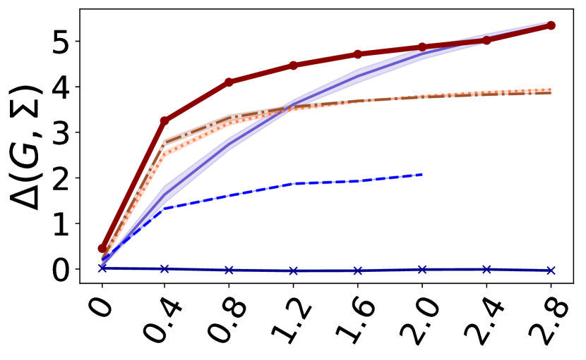
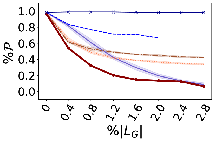
(a) Abortion

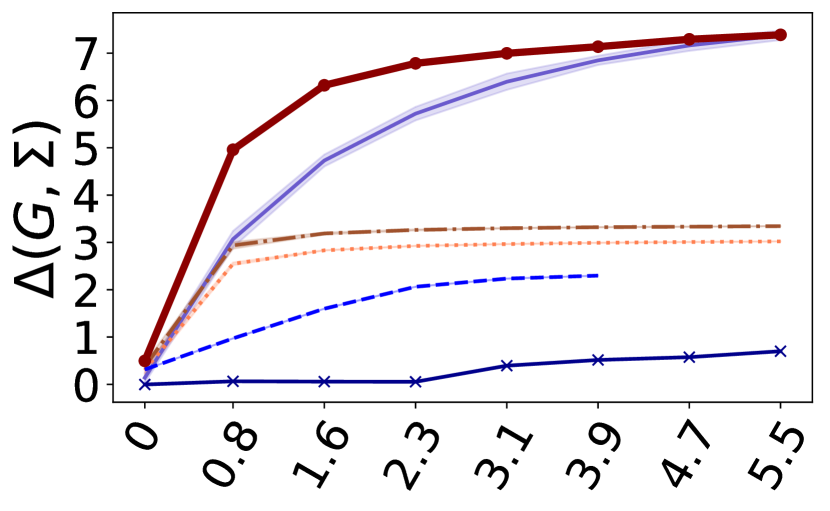
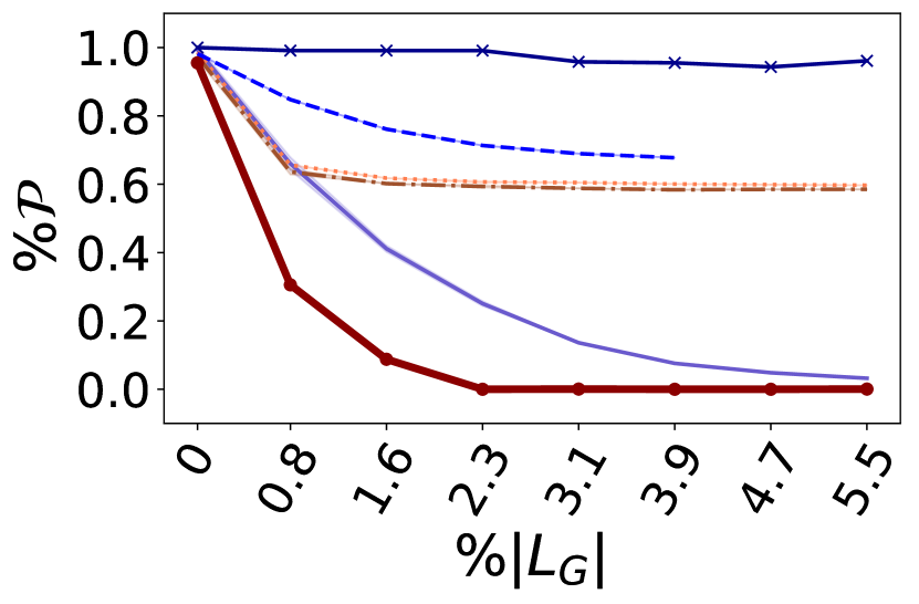
(b) MaTe

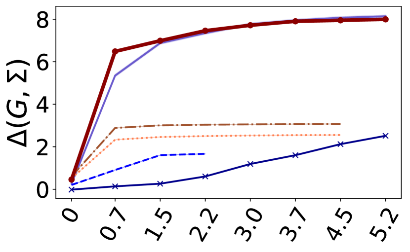
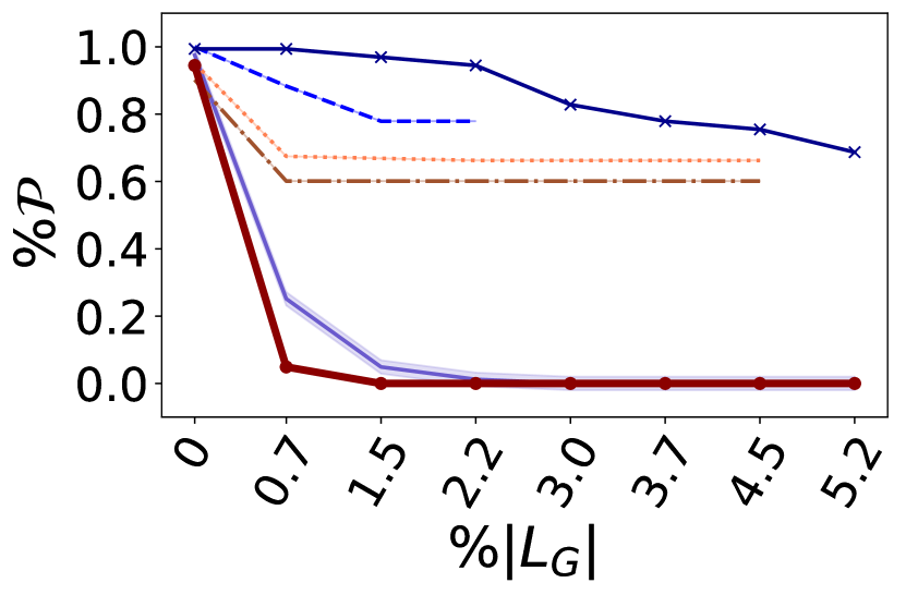
(c) MiHi

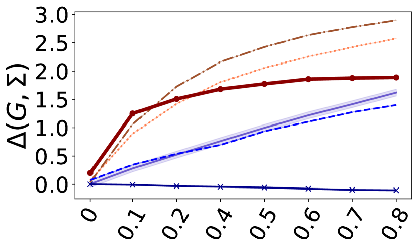
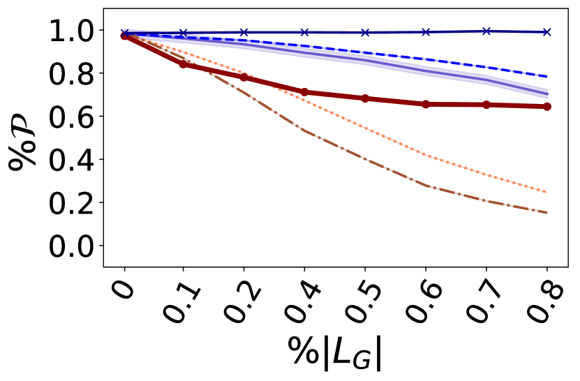
(d) PolBlogs

Figure 1. The first row shows the $\Delta(G,\Sigma)$ (y-axis) for increasing value of $k$, reported in terms of $\%\mathcal{L}_{G}$, the union of possible edges across $\mathcal{P}_{C}(G)$ and $\bar{C}$ for $C\in{R,B}$, (x-axis) for each algorithm. Higher values of $\Delta$ show more significant reduction of the structural bias. In the second row, we show the percentage of nodes that are still parochial, $\%\mathcal{P}=\frac{\lvert\mathcal{P}\left(G\right)\rvert-\lvert\mathcal{P}\left(G_{\mathrm{new}}\right)\rvert}{\lvert\mathcal{P}\left(G\right)\rvert}$ after $k$ additions.

Results of the experiments for different graphs. See the caption and the text for description of these results.

6. Experimental evaluation

The goal of our experimental evaluation is to understand how the addition of the set $\Sigma=\Sigma_{R}\cup\Sigma_{B}$ of $K=k_{R}+k_{B}$ edges output by RePBubLik+, run separately with $C=R$ and $B$, affects the structural bias of the network, by computing the gain in the structural bias reduction. In particular, we measure the gain with $\Delta(G,\Sigma)$, introduced in Sect. 5, used here with a simpler notation. We also measure the change $\lvert\mathcal{P}(G)\rvert-\lvert\mathcal{P}(G_{\mathrm{new}})\rvert$ after adding $\Sigma$.

Baselines. We compare RePBubLik+ to three different baselines (i.e., simplified variants of RePBubLik+) and to two existing algorithms, described in the following. The first baseline, PureRandom (PR) selects the source, and the target, nodes of the new edges uniformly at random from the set $\mathcal{P}_{C}(G)$ and $\bar{C}$, respectively. The second baseline Random Top-$N$ Central Nodes ($N$-RCN), given a parameter $N\in(0,100)$, sorts the nodes in $\mathcal{P}_{C}(G)$ by descending centrality, and picks, uniformly at random, $k_{C}$ edges with source in the top-$N$ percent of nodes in $\mathcal{P}_{C}(G)$. The last baseline, Random Top-$N$ Weighted Central Nodes ($N$-RWCN), differs from $N$-RCN as the nodes in $\mathcal{P}_{C}(G)$ are sorted in descending order by $\mathcal{R}(v)\times m_{v,u}$.

We compare RePBubLik+ also to two existing methods, ROV (Garimella et al., 2017a), and node2vec (Grover and Leskovec, 2016). The ROV algorithm outputs a set of $k$ edges to be added to $G$ to minimize the controversy score (RWC) (Garimella et al., 2018b). The RWC is a metric that characterizes how controversial a topic is by capturing how well separated the two colors are. ROV considers as candidates the edges between the high-degree vertices of each color (Garimella et al., 2017a, Algorithm 1). These edges are sorted by descending impact on the graph controversy score, and the top-$k$ edges are added to the graph. The objective of the comparison between ROV and RePBubLik+ is to verify whether an algorithm developed to minimize the RWC can be used to minimize the structural bias. node2vec is a graph embedding technique that encodes a network in a low-dimensional space retaining characteristics like the nodes’ similarity (Grover and Leskovec, 2016). The generation of the embedding is based on random walks. One of the main applications of node2vec is to employ the embedding as the feature space to train link recommendation algorithms. The goal of comparing node2vec to RePBubLik+ is to understand how the predictions of widely-used link recommendation algorithms affect the network’s structural bias. In the experiments, we create for each network a 128-dimensional space, then we train a logistic regression (avg. AUC 85%) over these features, and we predict the existence probabilities of edges from $\mathcal{P}(G)$. We add to the graph the top $k$ edges according to these probabilities.

Datasets. We create graphs obtained from Wikipedia, Amazon and PolBlogs. Table 1 shows the relevant statistics.

From Wikipedia we consider four bi-partitioned subgraphs related to controversial topics: politics, abortion, guns and sociology (Menghini et al., 2020). Each node in the graph is a page, and is assigned to one color according to Wikipedia’s categorization. Directed edges denote links, and are weighted using Wikipedia’s clickstream data.

The Amazon dataset contains metadata about books (Leskovec et al., 2007). Given two book categories, the vertices are all the items in those categories, colored accordingly. There is a directed edge $(u,v)$ if $v$ appears in the list of items similar to $u$. The edge is weighted by $v$’s sales rank. We built three graphs by considering pairs of the following categories: Mathematics & Technology (MaTe), History of Technology & Military Science (MiHi), and Mathematics & Astronomy (MaAs).

The Political Blogs dataset is a directed network of hyperlinks between weblogs on US politics (Adamic and Glance, 2005). Each node represents a blog and is colored according to its political leaning. Links between blogs were automatically extracted from a crawl of the front page of the blog and represent the edges of the graph. Each edge $(v,u)$ has weight proportional to the out-degree of $v$.

Wikipedia
Topic	$\lvert R\rvert$	$\lvert B\rvert$	$\lvert E\rvert_{R\rightarrow B}$	$\lvert E\rvert_{B\rightarrow R}$	$\lvert E\rvert$	%$\mathcal{P}_{R}(G)$	%$\mathcal{P}_{B}(G)$
Abort.	208	413	80	170	1911	85.56	89.20
Guns	142	118	72	79	723	82.95	71.69
Pol.	10347	10129	17452	16484	141486	25.97	42.36
Sociol.	602	2283	284	192	10514	91.32	96.36
Amazon
Topic	$\lvert R\rvert$	$\lvert B\rvert$	$\lvert E\rvert_{R\rightarrow B}$	$\lvert E\rvert_{B\rightarrow R}$	$\lvert E\rvert$	%$\mathcal{P}_{R}(G)$	%$\mathcal{P}_{B}(G)$
MaTe	827	566	25	42	675	90.91	79.63
MiHi	446	405	66	63	482	58.33	63.46
MaAs	827	294	11	6	680	97.31	95.15
PolBlogs
Topic	$\lvert R\rvert$	$\lvert B\rvert$	$\lvert E\rvert_{R\rightarrow B}$	$\lvert E\rvert_{B\rightarrow R}$	$\lvert E\rvert$	%$\mathcal{P}_{R}(G)$	%$\mathcal{P}_{B}(G)$
Politics	545	488	902	781	17348	87.71	90.37

Table 1. Networks’ statistics. The notation is consistent with the rest of the paper.

Setup. Given a network, we run RePBubLik and the other algorithms on that network for increasing values of $K$, with $K=1,2,4,6,\dotsc,400$ or $2000$ for larger graphs (Sociology and Politics). These values of $K$ represent only a small percentage of the set of possible edges to insert and correspond to the total number of edges to add to the graph. Once we set the value of K, accordingly, we allocate $k_{B}$ and $k_{R}$ of the $K$ edge insertions to each color proportionally to the sum of the BRs of the parochial vertices in each color. In particular, we define $Y_{C}=\sum_{v\in\mathcal{P}_{C}(G)}\mathsf{B}^{t}_{G}\left(v\right)$, for $C\in{R,B}$, then $k_{B}=\left\lceil k\frac{Y_{B}}{Y_{B}+Y_{R}}\right\rceil$ and $k_{R}=K-k_{B}$. This allocation strategy is a simple but reasonable heuristic that ensures that more edges are added from nodes whose color is more parochial.

We assign the weight $m_{v,u}=1/(d(v)+1)$ to the added edge $(v,u)$, where $d(v)$ is the out-degree of $v$ before the insertion, and then we re-normalize the weights of the other edges by multiplying each of them by $1-m_{v,u}$. Furthermore, we set $r=5$ and $b=2$. Moreover, for the algorithms picking the top-N central nodes $N=10$. To account for variability of the algorithm, we run them 10 times. The variance of the results is low, overall.

The code for our experiments is available from https://github.com/CriMenghini/RePBubLik.

Experiment results. In Fig. 1, the plots in the first row show how the structural bias is affected by the insertion of an incrementally larger set of edges, while the ones on the second row show the reduction in the number of parochial nodes. Each curve in the plot illustrates the gain by a different algorithm. We can draw the following observations. (1) RePBubLik+ performs better than the baselines and the competitors, especially after the insertion of a few edges, as they obtain much larger gain with fewer insertions, i.e., the average BR of parochial nodes decreases faster requiring less modifications. (2) N-RCN, N-WRC, and ROV after a certain point become flat. (3) Overall, RePBubLik+  is the best algorithm. (4) The values of RePBubLik+and PR converge, at different speed, to the same value when we add more edges. (5) node2vec, in the best cases, shows little improvement of the structural bias that, in the remaining cases, stays flat or even increases. We now explain these behaviours using the plots on the second row of Fig. 1.

(1) RePBubLik+ chooses edges that directly affect the BR of central nodes and, with a chain effect, the BR of nodes connected to them. More central are the nodes we attach the edges to, higher the structural bias drop is. In fact, it follows, as shown for all the networks, that the addition of even small set of edges is very effective. Additionally, we observe that the structural bias reduction corresponds to a significant drop of the number of parochial nodes.

(2) N-RCN, N-WRC, and ROV attach edges only to a subset of $\mathcal{P}(G)$ and as $k$ increases, so does the probability of adding multiple edges to the same nodes. These facts imply respectively that, especially on disconnected graphs (see MiHi in Fig. 1(c)), the addition of edges may affect few nodes, and that even the insertion of more edges does not modify the set of nodes on which the new edges have effect. Thus, the curves of N-RCN, N-WRCN and ROV reach an early saturation that expresses the scarce impact of subsequent edge additions. This explanation is confirmed by the percentage of parochial nodes, which does not decrease after the saturation point. Furthermore, the ROV shows a stepping behaviour due to it selecting edges between high-degree central nodes that minimize the RWC without imposing diversity constraints on nodes. And resulting in many selected edges being attached to the same node. Last, we see that on Polblogs the best algorithms are N-RCN, N-WRCN. This surprising superiority of the random approaches can be explained by the fact that Polblogs is a connected graph, thus edges added to the top-central nodes potentially affect all the nodes in $\mathcal{P}(G)$. Thus, even when N-RCN and N-WRCN add multiple new edges to the same set of nodes, $\Delta$ continues to increase.

(3) RePBubLik+  shows a consistent behaviour, indeed it increases the gain faster than other methods, requiring fewer insertions. The penalty factor $\eta$ allows the algorithm to diversify the set of nodes to which the new edges attach, raising the chances of lowering the BR of a larger number of parochial nodes, thus increasing the gain. This feature is important especially on disconnected graphs, where the vertices in tiny connected components always have lower centrality compared to those in huge ones. More importantly, we observe that the size of $\mathcal{P}(G)$ is often reduced to 0: RePBubLik+  is able to “heal” all the bad vertices, and if we measured the structural bias on the obtained graph it would be zero.

(4) The variants of RePBubLik: RePBubLik+ and PR, pick edges from the same candidate set, thus the more edges they can pick, the more likely they choose edges with similar effect, thus the average parochial nodes’ BR converges. This is the main explanation why the random algorithm performs so well.

(5) Generally, link recommendation algorithms tend to suggest edges between similar nodes. Node2vec captures this similarity through the nodes’ neighborhood. In this context, graphs partitions have high within- and low between-density. Nodes in the same partition then lie close in the embedding space. Edges suggested by node2vec with high probability connect nodes close to each other in the embedding, which often are in the same partition. Thus, node2vec has a hard time reducing the structural bias, and in some cases increases it.

Plots for guns, sociology, politics and MaAs show similar behaviour and can be found in App. A.

7. Conclusion

We presented RePBubLik, an algorithm that reduces the structural bias of a graph by adding $k$ edges. Thanks to the monotonicity and submodularity of the objective function, RePBubLik is able to return a constant-factor approximation using a greedy approach based on a task-specific variant of the random walk closeness centrality. The results of our experimental evaluation show that the edge insertions suggested by RePBubLik result in a much quicker decrease of the structural bias than existing methods and reasonable baselines.

The functionality of RePBubLik relies on the existence of an oracle receiving the network and a page in it as input and outputting the transition probabilities of potentially added links to the input page. We leave the question of designing an algorithm which learns such probabilities from data as future direction of this work.

Appendix A Missing proofs

We present here the proofs missing from the main body. For convenience, we repeat the statements of the lemmas.

*

Proof of Sect. 3.1.

We can write

$$\mathsf{r}^{t^{\prime}}\left(v;S\right)=t^{\prime}-\frac{1}{\lvert S\rvert}\sum_{w\in S}\mathbb{E}_{G}\left[T^{t^{\prime}}_{w}\left(v\right)\right]\enspace.$$

We apply Chebyshev’s inequality to the r.v. $\nicefrac{{1}}{{z}}\sum_{i=1}^{z}\bar{h}_{w_{i}}$, to bound the deviation from its expectation

$$\frac{1}{\lvert S\rvert}\sum_{w\in S}\mathbb{E}_{G}\left[T^{t^{\prime}}_{w}\left(v\right)\right]\enspace.$$

To get an upper bound to the variance of this r.v., we use the fact that the r.v.’s $\bar{h}_{w_{i}}$, $i=1,\dotsc,z$, are independent, and, from Popoviciu’s inequality, the fact that each has a variance at most $\nicefrac{{t^{\prime 2}}}{{4}}$, as $\bar{h}_{w_{i}}\in[0,t^{\prime}]$. ∎

The following result is used in the proof of Def. 4.1.

Lemma A.1 (Markov inequality for bounded random variables).

Let $X$ be a random variable satisfying $0\leq X\leq t$. We have:

$$\mathbb{P}(X\leq k)\leq\frac{t-\mathbb{E}\left[X\right]}{t-k}\enspace.$$

Proof.

It holds

$$\mathbb{E}\left[X\right] =\int_{0}^{k}xp(x)dx+\int_{k}^{t}xp(x)dx$$

$$\leq k\left(1-\mathbb{P}(X\geq k)\right)+t\mathbb{P}(X\geq k)\enspace.$$

Thus,

$$\mathbb{P}(X\geq k)\geq\frac{\mathbb{E}\left[X\right]-k}{t-k},$$

and

$$\mathbb{P}(X\leq k)=1-\mathbb{P}(X\geq k)\leq 1-\frac{\mathbb{E}\left[X\right]-k}{t-k}=\frac{t-\mathbb{E}\left[X\right]}{t-k}\enspace.\qed$$

*

Proof of Def. 4.1.

Assume first that $\mathsf{B}^{t}_{G}\left(v\right)\geq t(1-\nicefrac{{1}}{{8r}})$. Consider a set of $r$ independent random walkers, $w_{1},\dotsc,w_{r}$, each starting from $v$. We can see the trace of the partial walks taken by our random walker with restarts as the union of the traces of these walkers. The event $\mathcal{E}^{\prime}\doteq\text{``}\mathcal{T}_{v}\leq\nicefrac{{t}}{{2}}\text{''}$ is a strict subset of the event $\mathcal{E}^{\prime\prime}\doteq\text{``there is (at least) a walker }w_{i}$ for which $T_{v}^{t}\leq\nicefrac{{t}}{{2}}$”, as the condition in $\mathcal{E}^{\prime}$ implies the condition in $\mathcal{E}^{\prime\prime}$, but not vice versa. Thus, $\mathbb{P}(\mathcal{E}^{\prime})<\mathbb{P}(\mathcal{E}^{\prime\prime})$. By Lemma A.1 we have, for each walker, that

$$\mathbb{P}\left(T^{t}_{v}\leq\frac{t}{2}\right)\leq\frac{t-\mathbb{E}\left[T^{t}_{v}\left(S\right)\right]}{t-\frac{t}{2}}\leq\frac{\frac{t}{8r}}{\frac{t}{2}}\leq\frac{1}{4r}.$$

Thus, using the union bound over the $r$ walkers, we get $\Pr({\mathcal{E}}^{\prime\prime})\leq\nicefrac{{1}}{{4}}$. Equivalently $\mathbb{P}\left(\mathcal{T}_{v}\leq\nicefrac{{t}}{{2}}\right)\leq\nicefrac{{1}}{{4}}$.

For the case when $\mathsf{B}^{t}_{G}\left(v\right)\leq b$, using Markov inequality we get $\mathbb{P}\left(\mathcal{T}_{v}>4br\right)\leq\nicefrac{{1}}{{4}}$. ∎

*

Proof of Prob. 1.

We show an approximation-preserving polynomial time reduction from the minimum set cover problem to Prob. 1. Our reduction does not change the cost of the optimal solution, thus maintaining, in addition to NP-hardness, the APX-hardness.

Let $U=\{u_{1},u_{2},\dots,u_{n}\}$ be a domain and let $S_{1},S_{2},\dotsc,S_{m}$
$\subseteq U$ be an instance of the set cover problem. We construct an instance of Prob. 1 as follows. Fix $t\geq 3$. Let $V$ be union of the following sets: $U$, $S={\{s_{i}\}}_{i=1}^{m}$ representing the sets, $T=\bigcup_{j=1}^{m}T_{j}$ where each $T_{j}$ is a set of $\lceil t/2\rceil-1$ distinct vertices, and $\{g\}$. Assume all vertices except $g$ have color red and $g$ is blue. For each $i\in[n]$ and $j\in[m]$, place an edge from $u_{i}$ to $s_{j}$ if and only if $u_{i}\in S_{j}$. For each $j\in[m]$, using the vertices in $T_{j}$, place a path of length $\lceil t/2\rceil-1$ going from $s_{j}$ to $g$. For each $1\leq j\leq m$, it holds $\mathsf{B}^{t}_{G}\left(s_{j}\right)=\lceil\nicefrac{{t}}{{2}}\rceil-1$, and for each $1\leq i\leq n$,

$$\mathsf{B}^{t}_{G}\left(u_{i}\right)=\frac{1}{\lvert\{j\ :\ u_{i}\in S_{j}\}\rvert}\sum_{j\ \text{s.t.}\ u_{i}\in S_{j}}\mathsf{B}^{t}_{G}\left(s_{j}\right)+1=\lceil\nicefrac{{t}}{{2}}\rceil\enspace.$$

Clearly the bubble radius of vertices in $T$ is strictly less than $\nicefrac{{t}}{{2}}$. Thus the parochial vertices are all and only those in $U$. Assume there is a polynomial-time algorithm for Prob. 1. For any (optimal) solution $\Sigma\subseteq V\times V$, it holds $\mathsf{B}^{t}_{G_{\textrm{new}}}\left(u_{i}\right)<\nicefrac{{t}}{{2}}$ if and only if $\Sigma$ contains an edge whose source is in $\{u_{i}\}\cup\bigcup_{j\ \text{s.t.}\ u_{i}\in S_{j}}(\{s_{j}\}\cup T_{j})$, for each $i\in[n]$. The source vertices of the edges in $\Sigma$ must be distinct, as any solution containing two edges originating from the same vertex cannot be optimal. Denote with $Z$ the set of the source vertices of the edges in $\Sigma$. Consider now the solution $\Sigma^{\prime}$ obtained by changing (in polynomial time) $\Sigma$ as follows: 1. each edge in $\Sigma$ whose source is in $T_{i}$ is modified to have source $s_{i}$, for each $i\in[n]$; and 2. each edge in $\Sigma$ whose source is $u\in U$ is changed to have source $s_{j}$ where $j$ is such that $u\in S_{j}$. Clearly $\Sigma^{\prime}$ is still an (optimal) solution to Prob. 1. Let $\mathsf{OPT}$ be the set of source vertices of the edges in $\Sigma^{\prime}$. Clearly it must be $\mathsf{OPT}\subseteq S$. We now show that $\Sigma^{\prime}$ is an (optimal) solution to Prob. 1 if and only if $\mathsf{OPT}$ is such that $\{S_{j}\>\ s_{j}\in\mathsf{OPT}\}$ is a minimum set cover for the considered instance. It is evident that $\{S_{j}\ :\ s_{j}\in\mathsf{OPT}\}$ is a set cover, which can be obtained in polynomial time from $\Sigma^{\prime}$. We now show that this set cover is minimal. Consider now any set cover $Y\subseteq\{S_{1},\dotsc,S_{m}\}$, and consider the set of edges $\{(s_{i},g)\ :\ S_{i}\in Y\}$. Adding these edges to $G$ would result in all the vertices in $U$ to no longer be parochial. This holds in particular for any minimal set cover $Y$, from which we can create an (optimal) solution $\Sigma_{Y}$ to Prob. 1. Thus we found a bijection between (optimal) solutions to Prob. 1 and minimal set covers for the considered instance, and computing one from the other can be done in polynomial time, showing the NP-hardness of Prob. 1. The APX-hardness follows because, for any minimum set cover $Y$, the corresponding optimal solution $\Sigma_{Y}$ to Prob. 1, built as above, is such that $\lvert\Sigma_{Y}\rvert=\lvert Y\rvert$, thus if we had a constant-factor polynomial-time approximation algorithm for Prob. 1 we would have an algorithm with the same properties for the minimum set cover problem. ∎

*

Proof of Thm. 5.1.

Consider the probability space of all random walks starting from $v$ in $G_{\mathrm{new}}$ and $G$. We introduce a coupling between these two probability spaces as follows: consider a walk in $G_{\mathrm{new}}$ and couple every step of it to an identical step in $G$. If a walk in $G_{\mathrm{new}}$ never traverses $(v,w)$ then the gain function is zero as it gets coupled to the identical walk in $G$. Assume that the walk in $G_{\mathrm{new}}$ traverses $(v,w)$ at the $i$th step without first visiting a vertex in $\bar{C}_{v}$. Before traversing $(v,w)$, the two identical walks in $G_{\mathrm{new}}$ and $G$ have the same probabilities and the above coupling works. We partition the state space by conditioning on the step $i$ as follows:

Let $\mathcal{E}_{i}$, $1\leq i\leq t^{\prime}$, be the event that the walk in $G_{\mathrm{new}}$ traverses $(v,w)$ at step $i$. Consider all such walks, at step $i-1$ these walks need one more steps to reach the other color, and they are coupled to walks in $G$ which in expectation need $\mathsf{B}^{t^{\prime}-i+1}_{G}\left(v\right)$ steps to reach $\bar{C}_{v}$. Thus, assuming $\mathcal{E}_{i}$, the gain in bubble radius is equal to $\mathsf{B}^{t^{\prime}-i+1}_{G}\left(v\right)-1$.

Using the law of total expectation and summing over all $1\leq i\leq t^{\prime}$, we can write

(5) $$\Delta(G,v,(v,w),m_{vw},t^{\prime})=\sum_{i=1}^{t^{\prime}}\left(\mathsf{B}^{t^{\prime}-i+1}_{G}\left(v\right)-1\right)\mathbb{P}(\mathcal{E}_{i})\enspace.$$

The left hand side follows from the fact that $\mathbb{P}({\mathcal{E}}_{1})=m_{vw}$ and that $\mathsf{B}^{j}_{G}\left(v\right)\geq 1$ for any $1\leq j\leq t^{\prime}$. The right-hand side is concluded from the fact that $\mathsf{B}^{t^{\prime}-i+1}_{G}\left(v\right)\leq\mathsf{B}^{t^{\prime}}_{G}\left(v\right)$ and that

$$\sum_{i=1}^{t^{\prime}}\mathbb{P}(\mathcal{E}_{i})=\sum_{i=0}^{t^{\prime}-1}\Psi_{v}(i)m_{vw}=\mathcal{F}_{t^{\prime}}(v)m_{vw}\enspace.$$

∎

*

Proof of Thm. 5.1.

Using the law of total expectation, for any graph $Z$, it holds

$$\mathsf{B}^{t}_{Z}\left(u\right)= \left(\sum_{i=1}^{t-1}\left(i+\mathsf{B}^{t-i}_{Z}\left(v\right)\right)\mathbb{P}\left(u\binrel@{\rightsquigarrow}\binrel@@{\mathop{\kern 0.0pt\rightsquigarrow}\limits^{=i}_{Z}}v\right)\right)$$

$$+\mathbb{E}_{Z}\left[T^{t}_{u}\left(\bar{C}_{v}\right)\mid u\binrel@{\not\rightsquigarrow}\binrel@@{\mathop{\kern 0.0pt\not\rightsquigarrow}\limits^{<t}_{Z}}v\right]\mathbb{P}\left(u\binrel@{\not\rightsquigarrow}\binrel@@{\mathop{\kern 0.0pt\not\rightsquigarrow}\limits^{<t}_{Z}}v\right)\enspace.$$

Between $G$ and $G_{\mathrm{new}}$, we are only adding an outgoing edge from $v$ and modifying the weights of the edges outgoing from $v$, so

$$\mathbb{E}_{G}\left[T^{t}_{u}\left(\bar{C}_{v}\right)\mid u\binrel@{\not\rightsquigarrow}\binrel@@{\mathop{\kern 0.0pt\not\rightsquigarrow}\limits^{<t}_{G}}v\right]=\mathbb{E}_{G_{\mathrm{new}}}\left[T^{t}_{u}\left(\bar{C}_{v}\right)\mid u\binrel@{\not\rightsquigarrow}\binrel@@{\mathop{\kern 0.0pt\not\rightsquigarrow}\limits^{<t}_{G_{\mathrm{new}}}}v\right],$$

$$\mathbb{P}\left(u\binrel@{\not\rightsquigarrow}\binrel@@{\mathop{\kern 0.0pt\not\rightsquigarrow}\limits^{<t}_{G}}v\right)=\mathbb{P}\left(u\binrel@{\not\rightsquigarrow}\binrel@@{\mathop{\kern 0.0pt\not\rightsquigarrow}\limits^{<t}_{G_{\mathrm{new}}}}v\right),\ \text{and}\ \mathbb{P}\left(u\binrel@{\rightsquigarrow}\binrel@@{\mathop{\kern 0.0pt\rightsquigarrow}\limits^{=i}_{G}}v\right)=\mathbb{P}\left(u\binrel@{\rightsquigarrow}\binrel@@{\mathop{\kern 0.0pt\rightsquigarrow}\limits^{=i}_{G_{\mathrm{new}}}}v\right)\enspace.$$

Therefore,

$$\Delta(G,u,(v,w),m_{v},t) \doteq\mathsf{B}^{t}_{G}\left(u\right)-\mathsf{B}^{t}_{G_{\textrm{new}}}\left(u\right)$$

$$=\sum_{i=1}^{t-1}\left(\Delta(G,v,(v,w),m_{v},t-i)\right)\mathbb{P}\left(u\binrel@{\rightsquigarrow}\binrel@@{\mathop{\kern 0.0pt\rightsquigarrow}\limits^{=i}_{G}}v\right)$$

$$=\sum_{i=1}^{t-2}\left(\Delta(G,v,(v,w),m_{v},t-i)\right)\mathbb{P}\left(u\binrel@{\rightsquigarrow}\binrel@@{\mathop{\kern 0.0pt\rightsquigarrow}\limits^{=i}_{G}}v\right)\enspace.$$

The last step follows from the fact that $\Delta(G,v,(v,w),m_{v},1)=0$ because $\mathsf{B}^{1}_{Z}\left(u\right)=1$ for every vertex $u$ of any graph $Z$. ∎

We need the following technical result in successive proofs.

Lemma A.2.

If $\mathsf{B}^{t}_{G}\left(v\right)\geq\nicefrac{{t}}{{2}}$ then, for any $t^{\prime}\leq t$, it holds

$$\frac{t^{\prime}}{2}\leq\mathsf{B}^{t^{\prime}}_{G}\left(v\right)\leq t^{\prime}\enspace.$$

Proof.

The rightmost inequality is straightforward from the definition of $\mathsf{B}^{t^{\prime}}_{G}\left(v\right)$. Expanding the definition of $\mathsf{B}^{t}_{G}\left(v\right)$, it holds, for any $t^{\prime}<t$,

$$\mathsf{B}^{t}_{G}\left(v\right) =t\mathbb{P}\left(v\binrel@{\rightsquigarrow}\binrel@@{\mathop{\kern 0.0pt\rightsquigarrow}\limits^{\geq t}_{G}}\bar{C}_{v}\right)+\sum_{i=1}^{t-1}i\mathbb{P}\left(v\binrel@{\rightsquigarrow}\binrel@@{\mathop{\kern 0.0pt\rightsquigarrow}\limits^{=i}_{G}}\bar{C}_{v}\right)$$

$$\leq t\mathbb{P}\left(v\binrel@{\rightsquigarrow}\binrel@@{\mathop{\kern 0.0pt\rightsquigarrow}\limits^{\geq t}_{G}}\bar{C}_{v}\right)+t\mathbb{P}\left(v\binrel@{\rightsquigarrow}\binrel@@{\mathop{\kern 0.0pt\rightsquigarrow}\limits^{t^{\prime}\leq\cdot\leq t}_{G}}\bar{C}_{v}\right)+\sum_{i=1}^{t^{\prime}-1}i\mathbb{P}\left(v\binrel@{\rightsquigarrow}\binrel@@{\mathop{\kern 0.0pt\rightsquigarrow}\limits^{=i}_{G}}\bar{C}_{v}\right)$$

$$=t\mathbb{P}\left(v\binrel@{\rightsquigarrow}\binrel@@{\mathop{\kern 0.0pt\rightsquigarrow}\limits^{\geq t^{\prime}}_{G}}\bar{C}_{v}\right)+\sum_{i=1}^{t^{\prime}-1}i\mathbb{P}\left(v\binrel@{\rightsquigarrow}\binrel@@{\mathop{\kern 0.0pt\rightsquigarrow}\limits^{=i}_{G}}\bar{C}_{v}\right)\enspace.$$

Thus, since the l.h.s. is at least $\nicefrac{{t}}{{2}}$,

$$\frac{t}{2}\leq t\mathbb{P}\left(v\binrel@{\rightsquigarrow}\binrel@@{\mathop{\kern 0.0pt\rightsquigarrow}\limits^{\geq t^{\prime}}_{G}}\bar{C}_{v}\right)+\sum_{i=1}^{t^{\prime}-1}i\mathbb{P}\left(v\binrel@{\rightsquigarrow}\binrel@@{\mathop{\kern 0.0pt\rightsquigarrow}\limits^{=i}_{G}}\bar{C}_{v}\right),$$

i.e.,

$$\frac{1}{2}-\frac{1}{t}\sum_{i=1}^{t^{\prime}-1}i\mathbb{P}\left(v\binrel@{\rightsquigarrow}\binrel@@{\mathop{\kern 0.0pt\rightsquigarrow}\limits^{=i}_{G}}\bar{C}_{v}\right)\leq\mathbb{P}\left(v\binrel@{\rightsquigarrow}\binrel@@{\mathop{\kern 0.0pt\rightsquigarrow}\limits^{\geq t^{\prime}}_{G}}\bar{C}_{v}\right)\enspace.$$

By expanding $\mathsf{B}^{t^{\prime}}_{G}\left(v\right)$ in a similar way, and plugging in the last inequality above, we get

$$\mathsf{B}^{t^{\prime}}_{G}\left(v\right) =t^{\prime}\mathbb{P}\left(v\binrel@{\rightsquigarrow}\binrel@@{\mathop{\kern 0.0pt\rightsquigarrow}\limits^{\geq t^{\prime}}_{G}}\bar{C}_{v}\right)+\sum_{i=1}^{t^{\prime}-1}i\mathbb{P}\left(v\binrel@{\rightsquigarrow}\binrel@@{\mathop{\kern 0.0pt\rightsquigarrow}\limits^{=i}_{G}}\bar{C}_{v}\right)$$

$$\geq t^{\prime}\left(\frac{1}{2}-\frac{1}{t}\sum_{i=1}^{t^{\prime}-1}i\mathbb{P}\left(v\binrel@{\rightsquigarrow}\binrel@@{\mathop{\kern 0.0pt\rightsquigarrow}\limits^{=i}_{G}}\bar{C}_{v}\right)\right)+\sum_{i=1}^{t^{\prime}-1}i\mathbb{P}\left(v\binrel@{\rightsquigarrow}\binrel@@{\mathop{\kern 0.0pt\rightsquigarrow}\limits^{=i}_{G}}\bar{C}_{v}\right)$$

$$=\frac{t^{\prime}}{2}+\underbracket{\left(1-\frac{t^{\prime}}{t}\right)\sum_{i=1}^{t^{\prime}-1}i\mathbb{P}\left(v\binrel@{\rightsquigarrow}\binrel@@{\mathop{\kern 0.0pt\rightsquigarrow}\limits^{=i}_{G}}\bar{C}_{v}\right)}_{\geq 0}$$

$$\geq\frac{t^{\prime}}{2}\enspace.\qed$$

*

Proof of Thm. 5.1.

Using Thm. 5.1, we get

$$\Delta(G,\mathcal{P}_{C_{v}}\left(G\right),e,m_{e},t)=$$

(6) $$\frac{1}{\lvert\mathcal{P}_{C_{v}}\left(G\right)\rvert}\sum_{u\in\mathcal{P}_{C_{v}}\left(G\right)}\sum_{i=1}^{t-2}\Delta(G,v,e,m_{e},t-i)\mathbb{P}\left(u\binrel@{\rightsquigarrow}\binrel@@{\mathop{\kern 0.0pt\rightsquigarrow}\limits^{=i}_{G}}v\right)\enspace.$$

It holds from Thms. 5.1 and A.2 that

$$\Delta(G,v,e,m_{e},t^{\prime})\geq\left(\frac{t^{\prime}}{2}-1\right)m_{e}\ \text{for every}\ 1\leq t^{\prime}\leq t\enspace.$$

Using this fact, we can continue from (6) as follows

$$\Delta(G,\mathcal{P}_{C_{v}}\left(G\right),e,m_{e},t)$$

$$\geq\frac{1}{\lvert\mathcal{P}_{C_{v}}\left(G\right)\rvert}\sum_{u\in\mathcal{P}_{C_{v}}\left(G\right)}\sum_{i=1}^{t-2}\left(\frac{t-i}{2}-1\right)m_{e}\mathbb{P}\left(u\binrel@{\rightsquigarrow}\binrel@@{\mathop{\kern 0.0pt\rightsquigarrow}\limits^{=i}_{G}}v\right)$$

$$=\frac{m_{e}}{2}\underbracket{\frac{1}{\lvert\mathcal{P}_{C_{v}}\left(G\right)\rvert}\sum_{u\in\mathcal{P}_{C_{v}}\left(G\right)}\sum_{i=1}^{t-2}(t-i-2)\mathbb{P}\left(u\binrel@{\rightsquigarrow}\binrel@@{\mathop{\kern 0.0pt\rightsquigarrow}\limits^{=i}_{G}}v\right)}_{\mathsf{r}^{t-2}\left(v;\mathcal{P}_{C_{v}}\left(G\right)\right)},$$

which concludes the proof. ∎

*

Proof of Thm. 5.1.

It follows from Thm. 5.1 that, for any $t^{\prime}$,

$$\Delta(G,\mathrm{opt},e_{\mathrm{opt}},m_{\mathrm{opt}},t^{\prime}) \leq\mathcal{F}_{t^{\prime}}(u)\left(\mathsf{B}^{t^{\prime}}_{G}\left(\mathrm{opt}\right)-1\right)m_{\mathrm{opt}}$$

$$\leq(t^{\prime}-1)m_{\mathrm{opt}}\mathcal{F}_{t^{\prime}}(\mathrm{opt})\enspace.$$

By applying Thm. 5.1 first, and then the above inequality, we get

$$\Delta(G,\mathcal{P}_{C}\left(G\right),e_{\mathrm{opt}},m_{\mathrm{opt}},t)$$

$$\leq \frac{1}{\lvert\mathcal{P}_{C}\left(G\right)\rvert}\sum_{u\in\mathcal{P}_{C}\left(G\right)}\sum_{i=1}^{t-2}\left(\Delta(G,\mathrm{opt},e_{\mathrm{opt}},m_{\mathrm{opt}},t-i)\right)\mathbb{P}\left(u\binrel@{\rightsquigarrow}\binrel@@{\mathop{\kern 0.0pt\rightsquigarrow}\limits^{=i}_{G}}v\right)$$

$$\leq \frac{1}{\lvert\mathcal{P}_{C}\left(G\right)\rvert}\sum_{u\in\mathcal{P}_{C}\left(G\right)}\sum_{i=1}^{t-3}\left(\Delta(G,\mathrm{opt},e_{\mathrm{opt}},m_{\mathrm{opt}},t-i)\right)\mathbb{P}\left(u\binrel@{\rightsquigarrow}\binrel@@{\mathop{\kern 0.0pt\rightsquigarrow}\limits^{=i}_{G}}v\right)$$

$$\hskip 56.9055pt+\Delta(G,\mathrm{opt},e_{\mathrm{opt}},m_{\mathrm{opt}},2)\mathbb{P}\left(u\binrel@{\rightsquigarrow}\binrel@@{\mathop{\kern 0.0pt\rightsquigarrow}\limits^{=t-2}_{G}}v\right)$$

$$\leq \frac{1}{\lvert\mathcal{P}_{C}\left(G\right)\rvert}\sum_{u\in\mathcal{P}_{C}\left(G\right)}\sum_{i=1}^{t-3}(t-1-i)m_{\mathrm{opt}}\mathcal{F}_{t}(\mathrm{opt})\mathbb{P}\left(u\binrel@{\rightsquigarrow}\binrel@@{\mathop{\kern 0.0pt\rightsquigarrow}\limits^{=i}_{G}}v\right)+1$$

$$\leq \frac{1}{\lvert\mathcal{P}_{C}\left(G\right)\rvert}\sum_{u\in\mathcal{P}_{C}\left(G\right)}\sum_{i=1}^{t-2}2(t-2-i)m_{\mathrm{opt}}\mathcal{F}_{t}(\mathrm{opt})\mathbb{P}\left(u\binrel@{\rightsquigarrow}\binrel@@{\mathop{\kern 0.0pt\rightsquigarrow}\limits^{=i}_{G}}v\right)+1$$

$$\leq \ 2m_{\mathrm{opt}}\mathsf{r}^{t-2}\left(\mathrm{opt};\bar{C}_{\mathrm{opt}}\right)\mathcal{F}_{t}(\mathrm{opt})+1\leq 2m_{v}\mathsf{r}^{t-2}\left(v;\bar{C}_{\mathrm{opt}}\right)\gamma(G)+1$$

$$\leq \ (4\gamma(G)+1)\Delta(G,\mathcal{P}_{C}\left(G\right),e_{v},m_{v},t),$$

where the last step follows from Thm. 5.1. ∎

*

Proof of Thm. 5.1.

Let $G_{v}$ be the graph after adding only the edge $e_{v}$, $G_{u}$ be the graph after only adding the edge $e_{u}$, and $G_{vu}$ be the graph after adding both edges.

We first show the monotonicity of the objective function, i.e., that (3) holds. For any $w\in\mathcal{P}_{C}\left(G\right)$, it holds

$$\Delta(G,w,e_{v},m_{v},t) \doteq\mathsf{B}^{t}_{G}\left(w\right)-\mathsf{B}^{t}_{G_{v}}\left(w\right)$$

$$\leq\mathsf{B}^{t}_{G}\left(w\right)-\mathsf{B}^{t}_{G_{vu}}\left(w\right)$$

$$\doteq\Delta(G,w,\{e_{v},e_{u}\},\{m_{v},m_{u}\},t)$$

because $\mathsf{B}^{t}_{G_{v}}\left(w\right)\geq\mathsf{B}^{t}_{G_{vu}}\left(w\right)$, as adding an edge from $u$, which is in $C_{w}$, to a vertex in $\bar{C}_{w}$ cannot increase the bubble radius of $w$. The result generalizes to (3) in a straightforward way. We now show the sub-modularity of the objective function, i.e., that (4) holds. We start by showing that, for $w\in\mathcal{P}_{C}\left(G\right)$, it holds

$$\Delta(G,w,\{e_{v},e_{u}\},\{m_{v},m_{u}\},t)\leq \Delta(G,w,e_{v},m_{v},t)$$

$$+\Delta(G,w,e_{u},m_{u},t)\enspace.$$

With an expansion of the definition and a slight rearrangement of the terms, the above inequality is equivalent to

$$\underbracket{\mathsf{B}^{t}_{G_{v}}\left(w\right)-\mathsf{B}^{t}_{G_{vu}}\left(w\right)}_{\Delta(G_{v},w,e_{u},m_{u},t)}\leq\underbracket{\mathsf{B}^{t}_{G}\left(w\right)-\mathsf{B}^{t}_{G_{u}}\left(w\right)}_{\Delta(G,w,e_{u},m_{u},t)},$$

i.e., the gain of adding the same edge (in this case $e_{u}$) is smaller when the edge is added to a graph (in this case $G_{v}$) that has a superset of the edges (compared to $G$).

Consider all the walks from $w$ that either pass through $v$ or $u$. Among such walks, let $\mathcal{E}_{v}$ be the event of seeing $v$ first and $\mathcal{E}_{u}$ be the event of seeing $u$ first. If a walk does not pass through either $v$ or $u$, its probability of hitting the other color is the same in all graphs, as the graphs differ only in the outgoing edges from these two nodes and their weights. For the same reason, $\mathbb{P}(\mathcal{E}_{v})$ and $\mathbb{P}(\mathcal{E}_{u})$ do not change across the graphs. Thus,

$$\mathsf{B}^{t}_{G_{v}}\left(w\right)-\mathsf{B}^{t}_{G_{vu}}\left(w\right)=$$

$$\left(\mathbb{E}_{G_{v}}\left[T^{t}_{w}\left(\bar{C}_{w}\right)\mid\mathcal{E}_{v}\right]-\mathbb{E}_{G_{vu}}\left[T^{t}_{w}\left(\bar{C}_{w}\right)\mid\mathcal{E}_{v}\right]\right)\mathbb{P}(\mathcal{E}_{v})$$

$$+\left(\mathbb{E}_{G_{v}}\left[T^{t}_{w}\left(\bar{C}_{w}\right)\mid\mathcal{E}_{u}\right]-\mathbb{E}_{G_{vu}}\left[T^{t}_{w}\left(\bar{C}_{w}\right)\mid\mathcal{E}_{u}\right]\right)\mathbb{P}(\mathcal{E}_{u})\enspace.$$

Similarly,

$$\mathsf{B}^{t}_{G}\left(w\right)-\mathsf{B}^{t}_{G_{u}}\left(w\right)=$$

$$\left(\mathbb{E}_{G}\left[T^{t}_{w}\left(\bar{C}_{w}\right)\mid\mathcal{E}_{v}\right]-\mathbb{E}_{G_{u}}\left[T^{t}_{w}\left(\bar{C}_{w}\right)\mid\mathcal{E}_{v}\right]\right)\mathbb{P}(\mathcal{E}_{v})$$

$$+\left(\mathbb{E}_{G}\left[T^{t}_{w}\left(\bar{C}_{w}\right)\mid\mathcal{E}_{u}\right]-\mathbb{E}_{G_{u}}\left[T^{t}_{w}\left(\bar{C}_{w}\right)\mid\mathcal{E}_{u}\right]\right)\mathbb{P}(\mathcal{E}_{u})\enspace.$$

We want to show that it holds

$$\mathbb{E}_{G_{v}}\left[T^{t}_{w}\left(\bar{C}_{w}\mid\mathcal{E}_{v}\right)\right]-\mathbb{E}_{G_{vu}}\left[T^{t}_{w}\left(\bar{C}_{w}\mid\mathcal{E}_{v}\right)\right]$$

(7) $$\leq\mathbb{E}_{G}\left[T^{t}_{w}\left(\bar{C}_{w}\mid\mathcal{E}_{v}\right)\right]-\mathbb{E}_{G_{u}}\left[T^{t}_{w}\left(\bar{C}_{w}\mid\mathcal{E}_{v}\right)\right]\enspace.$$

and

$$\mathbb{E}_{G_{v}}\left[T^{t}_{w}\left(\bar{C}_{w}\mid\mathcal{E}_{u}\right)\right]-\mathbb{E}_{G_{vu}}\left[T^{t}_{w}\left(\bar{C}_{w}\mid\mathcal{E}_{u}\right)\right]$$

(8) $$\leq\mathbb{E}_{G}\left[T^{t}_{w}\left(\bar{C}_{w}\mid\mathcal{E}_{u}\right)\right]-\mathbb{E}_{G_{u}}\left[T^{t}_{w}\left(\bar{C}_{w}\mid\mathcal{E}_{u}\right)\right]\enspace.$$

We can write

$$\mathbb{E}_{G}\left[T^{t}_{w}\left(\bar{C}_{w}\right)\mid\mathcal{E}_{v}\right]$$

$$=\sum_{i=1}^{t}\left(i+\mathbb{E}_{G}\left[T^{t-i}_{v}\left(\bar{C}_{v}\right)\right]\right)\mathbb{P}\left(w\binrel@{\rightsquigarrow}\binrel@@{\mathop{\kern 0.0pt\rightsquigarrow}\limits^{=i}_{G}}v\mid\mathcal{E}_{v}\right)\enspace.$$

The probability on the right is the same on all graphs. Similar expressions hold for

$$\mathbb{E}_{G_{v}}\left[T^{t}_{w}\left(\bar{C}_{w}\right)\mid\mathcal{E}_{v}\right],\ \mathbb{E}_{G_{u}}\left[T^{t}_{w}\left(\bar{C}_{w}\right)\mid\mathcal{E}_{v}\right],\ \mathbb{E}_{G_{vu}}\left[T^{t}_{w}\left(\bar{C}_{w}\right)\mid\mathcal{E}_{v}\right],$$

and when conditioning on $\mathcal{E}_{u}$. To prove (7) and (8), we now show that, for every $t^{\prime}\leq t$, it holds

(9) $$\mathbb{E}_{G_{v}}\left[T^{t^{\prime}}_{v}\left(\bar{C}_{v}\right)\right]-\mathbb{E}_{G_{vu}}\left[T^{t^{\prime}}_{v}\left(\bar{C}_{v}\right)\right]\leq\mathbb{E}_{G}\left[T^{t^{\prime}}_{v}\left(\bar{C}_{v}\right)\right]-\mathbb{E}_{G_{u}}\left[T^{t^{\prime}}_{v}\left(\bar{C}_{v}\right)\right],$$

and

$$\mathbb{E}_{G_{v}}\left[T^{t^{\prime}}_{u}\left(\bar{C}_{u}\right)\right]-\mathbb{E}_{G_{vu}}\left[T^{t^{\prime}}_{u}\left(\bar{C}_{u}\right)\right]\!\leq\!\mathbb{E}_{G}\left[T^{t^{\prime}}_{u}\left(\bar{C}_{u}\right)\right]-\mathbb{E}_{G_{u}}\left[T^{t^{\prime}}_{u}\left(\bar{C}_{u}\right)\right].$$

We focus on showing (9), as the same steps, with simple modifications, can be followed to show the other inquality. For $Z\in\{G,G_{u},G_{v},G_{vu}\}$, let $\mathcal{A}_{Z}$ be the event that a random walk starting at $v$ reaches $u$ in at most $t$ steps before visiting any vertex in $\bar{C}_{v}$, and let $\bar{\mathcal{A}}_{Z}$ be the complementary event. It holds

$$\mathbb{P}(\mathcal{A}_{G_{v}})=\mathbb{P}(\mathcal{A}_{G_{vu}})\leq\mathbb{P}(\mathcal{A}_{G})=\mathbb{P}(\mathcal{A}_{G_{u}}),$$

due to the insertion of $e_{v}$. It also holds

$$\mathbb{E}_{G_{v}}\left[T^{t^{\prime}}_{v}\left(\bar{C}_{v}\right)\mid\bar{\mathcal{A}}_{G_{v}}\right]=\mathbb{E}_{G_{vu}}\left[T^{t^{\prime}}_{v}\left(\bar{C}_{v}\right)\mid\bar{\mathcal{A}}_{G_{vu}}\right],$$

and

$$\mathbb{E}_{G}\left[T^{t^{\prime}}_{v}\left(\bar{C}_{v}\right)\mid\bar{\mathcal{A}}_{G}\right]=\mathbb{E}_{G_{u}}\left[T^{t^{\prime}}_{v}\left(\bar{C}_{v}\right)\mid\bar{\mathcal{A}}_{G_{u}}\right],$$

Using the law of total expectation (across $\mathcal{A}_{Z}$ and $\bar{\mathcal{A}}_{Z}$) and applying these facts, we can rewrite (9) as

$$\left(\mathbb{E}_{G_{v}}\left[T^{t^{\prime}}_{v}\left(\bar{C}_{v}\right)\mid\mathcal{A}_{G_{v}}\right]-\mathbb{E}_{G_{vu}}\left[T^{t^{\prime}}_{v}\left(\bar{C}_{v}\right)\mid\mathcal{A}_{G_{vu}}\right]\right)\mathbb{P}(\mathcal{A}_{G_{v}})$$

$$\leq \left(\mathbb{E}_{G}\left[T^{t^{\prime}}_{v}\left(\bar{C}_{v}\right)\mid\mathcal{A}_{G}\right]-\mathbb{E}_{G_{u}}\left[T^{t^{\prime}}_{v}\left(\bar{C}_{v}\right)\mid\mathcal{A}_{G_{u}}\right]\right)\mathbb{P}(\mathcal{A}_{G})\enspace.$$

The differences between parentheses have the same value, as their corresponding terms have the same values. The inequality holds because $\mathbb{P}(\mathcal{A}_{G_{v}})\leq\mathbb{P}(\mathcal{A}_{G})$ due to the insertion of $e_{v}$ in $G$ to obtain $G_{v}$.

∎

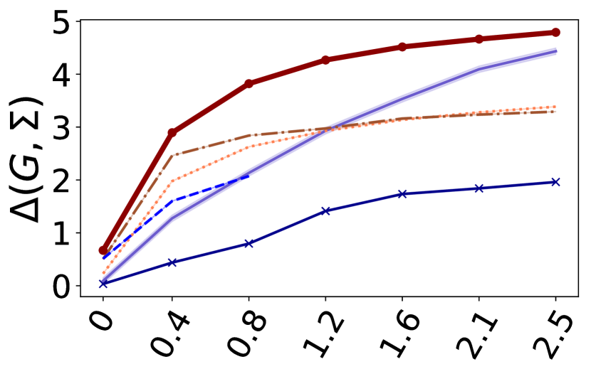
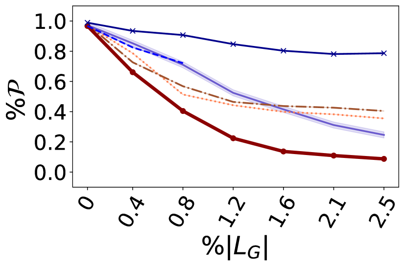
(a) Guns

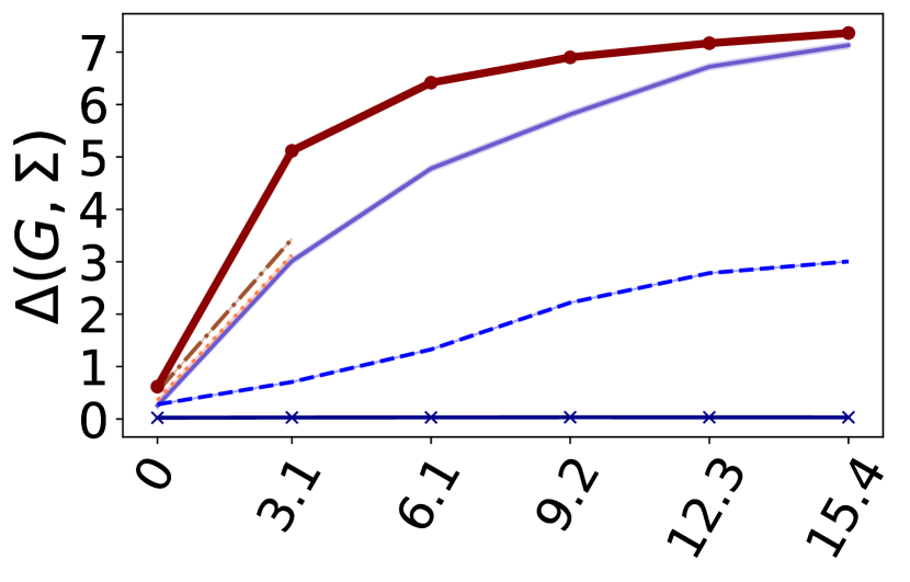
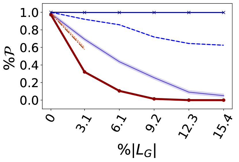
(b) MaAs

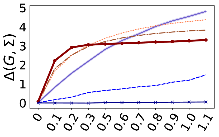
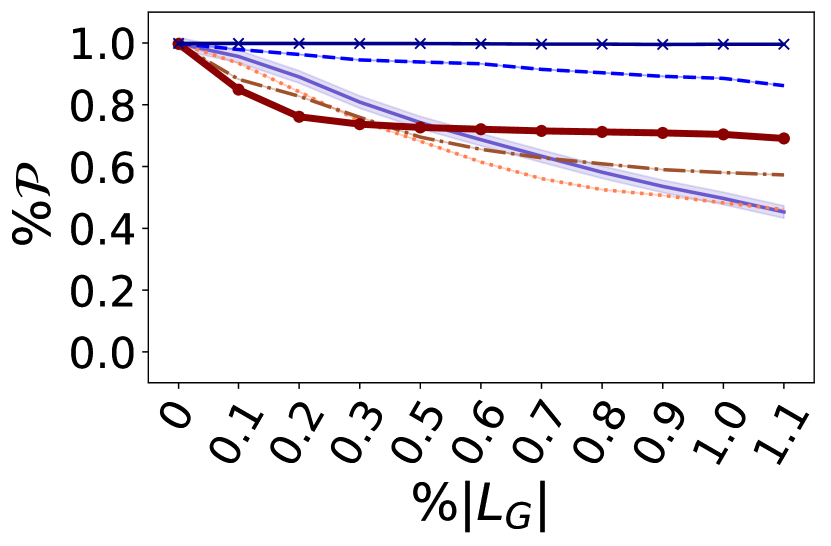
(c) Sociology

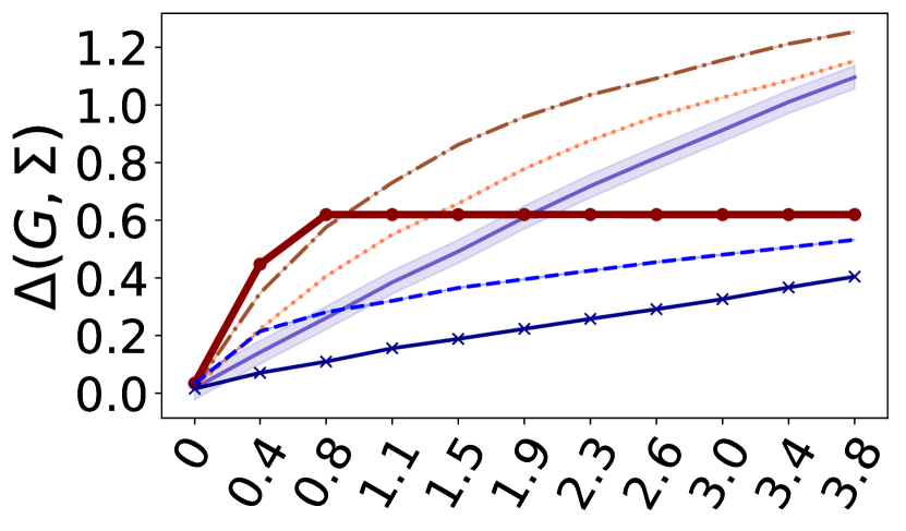
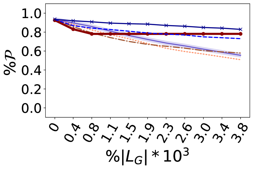
(d) Politics

Figure 2. The first row shows the $\Delta(G,\Sigma)$ (y-axis) for increasing value of $k$, reported in terms of $\%\mathcal{L}_{G}$, the union of possible edges across $\mathcal{P}_{C}(G)$ and $\bar{C}$ for $C\in{R,B}$, (x-axis) for each algorithm. Higher values of $\Delta$ show more significant reduction of the structural bias. In the second row, we show the percentage of nodes that are still parochial, $\%\mathcal{P}=\frac{\lvert\mathcal{P}\left(G\right)\rvert-\lvert\mathcal{P}\left(G_{\mathrm{new}}\right)\rvert}{\lvert\mathcal{P}\left(G\right)\rvert}$ after $k$ additions.

Results of the experiments for different graphs. See the caption and the text for description of these results.