A hot mini-Neptune in the radius valley orbiting solar analogue HD 110113

Abstract

We report the discovery of HD 110113 b (TOI-755.01), a transiting mini-Neptune exoplanet on a 2.5-day orbit around the solar-analogue HD 110113 ($T_{\rm eff}$= $5730$K). Using TESS photometry and HARPS radial velocities gathered by the NCORES program, we find HD 110113 b has a radius of $2.05\pm 0.12$  R_⊕ and a mass of $4.55\pm 0.62$  M_⊕. The resulting density of $2.90^{+0.75}_{-0.59}$  g cm^-3 is significantly lower than would be expected from a pure-rock world; therefore, HD 110113 b must be a mini-Neptune with a significant volatile atmosphere. The high incident flux places it within the so-called radius valley; however, HD 110113 b was able to hold onto a substantial (0.1-1%) H-He atmosphere over its $\sim 4$Gyr lifetime. Through a novel simultaneous gaussian process fit to multiple activity indicators, we were also able to fit for the strong stellar rotation signal with period $20.8\pm 1.2$  d from the RVs and confirm an additional non-transiting planet with a mass of $10.5\pm 1.2$  M_⊕ and a period of $6.744^{+0.008}_{-0.009}$  d.

1 Introduction

Since its launch in 2018, NASA’s TESS mission has attempted to detect small transiting planets around bright, nearby stars amenable to confirmation with radial velocity observations (Ricker et al., 2016). The HARPS spectrograph on the 3.6m telescope at La Silla, Chile (Mayor et al., 2003) has been deeply involved in this follow-up effort, beginning with its first detection, the hot super-Earth Pi Mensae c (Huang et al., 2018), and continuing with the first multi-planet system (TOI-125 Quinn et al., 2019; Nielsen et al., 2020),

This unique combination of space-based photometry (which provides planetary radius) and precise radial velocities (which provide planetary mass) also allows for the determination of exoplanet densities, and, therefore, an insight into the internal structure of worlds outside our solar system. These analyses have revealed a diversity of planet structures in the regime between Earth and Neptune, from high-density evaporated giant planet cores like TOI-849b (5.2 g cm^-3 Armstrong et al., 2020), to low-density mini-Neptunes such as TOI-421 c (Carleo et al., 2020), as well as planets which follow a more linear track from rocky super-earths to Neptunes dominated by gaseous envelopes, such as the two inner planets orbiting $\nu^{2}$ Lupi (Kane et al., 2020) and TOI-735 (Cloutier et al., 2020; Nowak et al., 2020).

The detection of exoplanets with well-constrained physical parameters can also lead to the discovery of statistical trends within the planet population which encode information on planetary formation and evolution. The "valley" seen around $1.8$ R_⊕ in Kepler data (Fulton et al., 2017; Van Eylen et al., 2018) is one such feature. According to current theory planets that first formed with gaseous envelopes within this valley have, due to heating from either their stars (e.g. evaporation, Owen & Wu, 2017) or from internal sources (e.g. core-powered mass loss, Ginzburg et al., 2018), lost those initial gaseous envelopes, thereby evolving to significantly smaller radii to become "evaporated cores". By observing the physical parameters of small, hot exoplanets, the exact mechanisms of this process can be revealed.

In this paper, we present the detection, confirmation and RV characterisation of two exoplanets orbiting the star HD 110113 — the hot mini-Neptune HD 110113 b and the non-transiting HD 110113 c. The observations from which these planets were detected are described in section 2, while the analysis of that data is described in section 3. In section 4 we discuss the validity of the outer planet RV signal (4.1), whether HD 110113 is a solar analogue (4.2) the internal structure and evaporation of planet b (4.3 & 4.4), and potential future observations of the system (4.5). We summarize our conclusions in section 5.

2 Observations

2.1 TESS photometry

HD 110113 was observed during TESS sector 10 with 2-minute cadence for 22.5 days, excluding a 2.5 day gap between TESS orbits to downlink data. The lightcurve was extracted using the SPOC (Science Processing Operations Centre; Jenkins et al., 2016) SAP (simple aperture photometry) pipeline. It was then processed using the Pre-Search Data Conditioning (PDC, Stumpe et al., 2012; Smith et al., 2012; Stumpe et al., 2014) pipeline, producing precise detrended photometry with typical precision of 150 ppm/hr for this star, and then searched for exoplanetary candidates with the Transiting Planet Search (TPS; Jenkins et al., 2010). This identified a strong candidate with a period of 2.54 d, a depth of only 410 ppm and a Signal to Noise Ratio (SNR) of 7.6. Automated and human vetting subsequently designated this candidate a planet candidate and it was assigned TESS Object of Interest (TOI) 755.01.

We inspected the TESS aperture using tpfplotter (plotted in Figure 1; Aller et al., 2020) to ensure no nearby contaminant stars could be causing the transit. We found five stars within the aperture with contrast less than 8 mag, with the brightest with a $\Delta{\rm mag}$ of only 3.5. However, to cause the observed 410 ppm transit, this star would need to host eclipses of at least 1%. Furthermore, being more than 1.2 pix, and therefore almost one full-width-half-maximum (FWHM) of the point-spread function (PSF), away from the target star, we would expect to see a significant centroid shift. However, the SPOC data validation modelling (Twicken et al., 2018; Li et al., 2019) shows no such shift and suggests the transit occurs within 0.25 pixels from the target position. The other stars present are also $>1$ pixel away, and are increasingly fainter ($\Delta{\rm mag}$ of 6.9–7.9), requiring eclipse depths of 25–75%. Causing the observed transit with such a blend scenario therefore becomes increasingly unlikely given the flat-bottomed transit shape of TOI-755.01. We conclude that a blend scenario from a known contaminant is unlikely, however we pursue additional photometry to confirm.

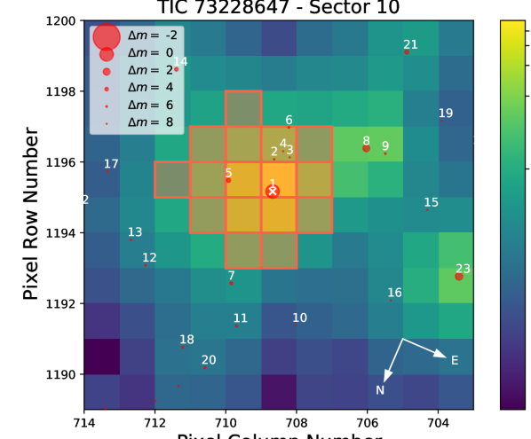
Figure 1: TESS photometric aperture plotted with tpfplotter (Aller et al., 2020). The default TESS aperture used by SAP is overplotted in red, and nearby stars down to $\Delta{\rm mag}=8$ from Gaia DR2 (Brown et al., 2018) are plotted as red circles. The target HD 110113 is marked with a white cross.

2.2 Ground-based Photometric Follow-up

We observed a full transit of TOI-755.01 continuously for 443 minutes in Pan-STARSS $z$-short band on UTC 2020 March 13 from the LCOGT (Brown et al., 2013) 1-m network node at Cerro Tololo Inter-American Observatory. The $4096\times 4096$ LCOGT SINISTRO cameras have an image scale of $0\aas@@fstack{\prime\prime}389$ per pixel, resulting in a $26\arcmin\times 26\arcmin$ field of view. The images were calibrated by the standard LCOGT BANZAI pipeline (McCully et al., 2018). Photometric data were extracted using AstroImageJ (Collins et al., 2017). The mean stellar PSF in the image sequence had a FWHM of $2\aas@@fstack{\prime\prime}8$. Circular apertures with radius $3\aas@@fstack{\prime\prime}1$ were used to extract the differential photometry.

The TOI-755 SPOC pipeline transit depth of 397 ppm is too shallow to reliably detect with ground-based observations, so we instead checked for possible nearby eclipsing binaries (NEBs) that could be contaminating the irregularly shaped SPOC aperture that generally extends $\sim 1\arcmin$ from the target star. To account for possible contamination from the wings of neighboring star PSFs, we searched for NEBs out to $2\aas@@fstack{\prime}5$ from the target star. If fully blended in the SPOC aperture, a neighboring star that is fainter than the target star by 8.54 magnitudes in TESS-band could produce the SPOC-reported flux deficit at mid-transit (assuming a 100% eclipse). To account for possible delta-magnitude differences between TESS-band and Pan-STARSS $z$-short band, we searched an extra 0.5 magnitudes fainter (down to TESS-band magnitude 18.5).

The brightness and distance limits resulted in a search for NEBs in 90 Gaia DR2 stars, which includes all stars marked in red in Figure 1 and a further 67 contaminants with $\Delta{\rm mag}>8$. We estimated the expected NEB depth in each neighboring star by taking into account both the difference in magnitude relative to TOI-755 and the distance to TOI-755 (to account for the estimated fraction of the star’s flux that would be contaminating the TOI-755 SPOC aperture). If the RMS of the 10-minute binned light curve of a neighboring star is more than a factor of 3 smaller than the expected NEB depth, we consider an NEB to be tentatively ruled out in the star over the observing window. We then visually inspect each neighboring star’s light curve to ensure no obvious eclipse-like signal. The LCOGT data rule out possible contaminating NEBs at the SPOC pipeline nominal ephemeris and over a -$1.7\sigma$ to +$2.3\sigma$ ephemeris uncertainty window. By process of elimination, we conclude that the transit is indeed occurring in TOI-755, or a star so close to TOI-755 that it was not detected by Gaia DR2, or the event occurred outside our observing window.

2.3 Ground-based Archival Photometry

Although detecting the transits of HD 110113 b required precise space-based photometry, ground-based photometric surveys have observed HD 110113 and can provide constraints on stellar variability, and therefore an independent measure of the stellar rotation period.

WASP-South was a wide-field array of 8 cameras forming the Southern station of the WASP transit-search survey (Pollacco et al., 2006). The field of HD 110113 was observed over 150-night spans in each of 2007 and 2008, and then again over 2011 and 2012, acquiring a total of 30 000 photometric data points. WASP-South was at that time equipped with 200-mm, f/1.8 lenses, observing with a 400–700 nm passband, and with a photometric extraction aperture of 48 arcsecs. There are other stars in the aperture around HD 110113, but the brightest has $\Delta{\rm mag}=3$ while the others have $\Delta{\rm mag}>5$. Therefore any rotation signal is likely from HD 110113. We searched the data for rotational modulations using the methods from Maxted et al. (2011).

The data from 2011 and 2012 show a modulation at a period of 21 $\pm$ 2 d (see Figure 2). This is significant at the 1% false-alarm level with an amplitude of 2 mmag, both in each year separately, and when the data from the two years are combined. The data from 2007 and 2008 combined show a significant modulation at twice this period of $\sim 42$ $\pm$ 4 d. There is also power near 21 d in the 2007/2008 periodogram, but it is not significant in its own right. Although it would seem more likely from these data alone that the rotational period of HD 110113 is 42 $\pm$ 4 days, with the $21$ d period coming from the first harmonic, the WASP data cannot on its own distinguish between these two possible periods.

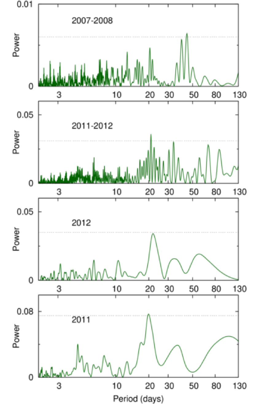
Figure 2: Periodograms of the WASP-South data for TOI-755. The top panel shows data from 2007 & 2008 combined, with a significant 42-d periodicity. The lower panels show data from 2011 & 2012, separately and combined, which show more strongly a periodicity of 21-d. The dotted horizontal lines are the estimated 1%-likelihood false-alarm levels.

2.4 High-resolution imaging

High-angular-resolution imaging is needed to search for nearby sources that can contaminate the TESS photometry, resulting in an underestimated planetary radius, or that can be the source of astrophysical false positives, such as background eclipsing binaries. Through the TESS Follow-Up Program (TFOP), three such images were obtained across two telescopes, with the results shown in Figure 3.

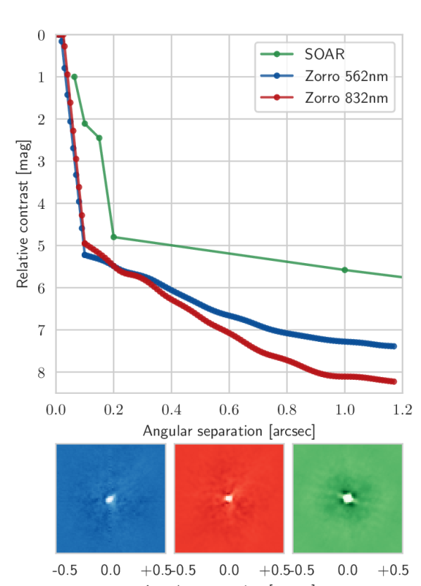
Figure 3: Contrast curves and images from Gemini/Zorro (blue & red for 562 and 832nm respectively), and SOAR (green).

2.4.1 SOAR

We searched for stellar companions to TOI-755 with speckle imaging on the 4.1-m Southern Astrophysical Research (SOAR) telescope (Tokovinin, 2018) on 14 July 2019 UT, observing in Cousins I-band, a similar visible bandpass as TESS. More details of the observation are available in Ziegler et al. (2020). The $5\sigma$ detection sensitivity and speckle auto-correlation functions from the observations are shown in Figure 3. No nearby stars with magnitudes brighter than $I=16$ were detected within 3″ of HD 110113 in the SOAR observations.

2.4.2 Gemini/Zorro

High-resolution speckle interferometric images of HD 110113 were obtained on 14 January 2020 UT using the Zorro instrument mounted on the 8-meter Gemini South telescope located on the summit of Cerro Pachon in Chile. Zorro simultaneously observes in two bands, (832 nm & 562 nm with widths of 40 & 54 nm respectively), obtaining diffraction-limited images with inner working angles 0.017 and 0.028 arcsec, respectively. The observation consisted of 3-minute sets of 1000$\times$0.06-second images. All the images were combined and subjected to Fourier analysis, leading to the production of final data products, including speckle reconstructed imagery (see Howell et al., 2011). Figure 3 shows the $5\sigma$ contrast curves in both filters for the Zorro observation and includes an inset showing the 832 nm reconstructed image. The resulting contrast limits reveal that HD 110113 is a single star to contrast limits of 5 to 8 magnitudes, ruling out most main sequence companions to the star within the spatial limits of $\sim$11 to 320 au (for $d=106.3$pc).

2.5 HARPS High Resolution Spectroscopy

Over the course of two observing seasons in 2018 and 2019, a total of 114 high-resolution spectra were taken with the High Accuracy Radial velocity Planet Searcher (HARPS, Pepe et al., 2002; Mayor et al., 2003) on the ESO 3.4m telescope at La Silla, Chile. These spectra were taken as part of the NCORES program (PI:Armstrong, 1102.C-0249) designed to specifically study the internal structure of hot worlds.

We used the high-accuracy mode of HARPS with a $1\arcsec$ science fibre on the star and a second on-sky fibre monitoring the background flux during exposure. The nominal exposure time was 1800 seconds, with a few exceptions of slightly longer or shorter integration, depending on observing conditions and schedule.

Spectra and RV information were extracted using the offline HARPS data reduction pipeline hosted at Geneva Observatory. We use a flux template matching a G1 star to correct the continuum-slope in each echelle order. The spectra were cross correlated with a binary G2 mask to derive the cross correlation function (CCF) (Baranne et al., 1996), on which we fit a Gaussian function to obtain RVs, FWHM and contrast. Additionally, we compute the bisector-span (Queloz et al., 2001) of the CCF and spectral indices tracing chromospheric activity (Gomes da Silva et al., 2011; Boisse et al., 2009).

We reach a typical SNR per pixel of 75 (order 60, 631nm) in individual spectra, corresponding to an RV error of 1.41m s^-1. The HARPS spectra and derived RVs were accessed and downloaded through the DACE portal hosted at the University of Geneva (Buchschacher et al., 2015) under the target name HD 110113.

3 Analysis

3.1 Stellar Parameters

Parameter	Value	Parameter	Value
TOI ID	TOI-755	R.A. [∘]	$190.0365636$ a
TIC ID	73228647 b	R.A. [hms]	12:40:08.78 a
HD	HD 110113	Dec. [∘]	$-44.3120777$ a
HIP	HIP 61820	Dec. [dms]	-44:18:43.48 a
Gaia ID	6133384959942131968a	$\delta{\rm RA}$ [mas ${\rm yr}^{-1}$]	$-3.72\pm 0.1$ a
$\pi{}[{\rm mas}]$	$9.38\pm 0.036$ a	$\delta{\rm DEC}$ [mas ${\rm yr}^{-1}$]	$-13.68\pm 0.12$ a
$d$ [pc]	$106.3\pm 0.72$ e	$R_{s}$ [$R_{\odot}$]	$0.968\pm 0.018$ e
B	$10.71\pm 0.032$ c	$M_{s}$ [$M_{\odot}$]	$0.997\pm 0.06$ e
V	$10.063\pm 0.027$ c	$\log g$	$4.46\pm 0.05$ e
Gaia $G$	$9.91\pm 0.0004$ a	$T_{\rm eff}$ [K]	$5732\pm 50$ e
TESS mag	$9.4628\pm 0.006$ b	$\rm[Fe/H]$	$0.14\pm 0.02$ e
J	$8.903\pm 0.037$ c	$v\sin{i}$ [km s-1]	$1.74\pm 0.15$ e
H	$8.594\pm 0.063$ c	$P_{\rm rot}$ [d]	$20.8\pm 1.2$ f
K	$8.502\pm 0.024$ c	Age $[{\rm Gyr}]$	4.0 $\pm$ 0.5 Gyr g

Table 1: Stellar parameters. ^a From Gaia DR2(Brown et al., 2018). ^b From the TESS Input Catalogue v8 (Stassun et al., 2019). ^c Johnson magnitudes from APASS (Henden et al., 2015). ^d From 2MASS (Skrutskie et al., 2006). ^e Derived from HARPS spectra and archival data - see sect 3.1.1. ^f Determined using the GP fit to activity indicators and RVs as described in 3.2.1. ^g Derived from $[\rm{Y}/\rm{Al}]$ abundance-age relation as described in sect 3.1.2.

3.1.1 Global Stellar Parameters

The star’s effective temperature ($T_{\rm eff}$), surface gravity ($\log g$), and metallicity ($\rm[Fe/H]$) were derived using a recent version of the MOOG code (Sneden, 1973) and a set of plane-parallel ATLAS9 model atmospheres (Kurucz, 1993). The analysis was done in LTE. The methodology used is described in detail in Sousa et al. (2011) and Santos et al. (2013a). The full spectroscopic analysis is based on the Equivalent Widths (EWs) of 233 Fe i@ and 34 Fe ii@ weak lines by imposing ionization and excitation equilibrium. The line-list used was taken from Sousa et al. (2008). We obtained resulting parameters of $T_{\rm eff}$=$5732\pm 16$K, $\log g$$=4.46\pm 0.05$ and $\rm[Fe/H]$$=0.14\pm 0.02$. To account for potential systematic uncertainties, we increased the error bars to $50$K and 0.05 dex for $T_{\rm eff}$ and $\log g$ respectively.

To constrain the physical stellar parameters of HD 110113 given the observed information, we applied three techniques.

The first technique was to use the main-sequence calibrations of Torres et al. (2010) which derive $R_{s}$ and $M_{s}$ using polynomial functions of $T_{\rm eff}$, $\log g$ and $\rm[Fe/H]$, which are built using the observed properties of calibration stars. Uncertainties were propagated using 10000 Monte Carlo draws and the mass was corrected using the calibration of Santos et al. (2013b). This produced a mass and radius of $0.989\pm 0.01$  $M_{\odot}$ and $0.998\pm 0.025$  $R_{\odot}$ respectively, although Torres et al. (2010) suggest minimum uncertainties of 0.06$M_{\odot}$ and 0.03$R_{\odot}$ respectively.

The second was using theoretical isochrones (MIST, Choi et al., 2016) as well as observed properties (e.g. colours) to constrain stellar parameters, which we performed using isoclassify (Huber, 2017; Berger et al., 2020). Inputs included the derived spectral properties $T_{\rm eff}$, $\log g$ and $\rm[Fe/H]$, as well as archival data for HD 110113 including APASS B & V magnitudes (Henden et al., 2015), Gaia parallax, Gp, Rp, Bp and luminosity (Brown et al., 2018), SkyMapper ugriz observations (Onken et al., 2020) and 2MASS JHK observations (Skrutskie et al., 2006). This resulted in a mass & radius of $1.004^{+0.042}_{-0.047}$  $M_{\odot}$ and $1.002\pm 0.028$  $R_{\odot}$ respectively. The well-constrained nature of the input measurements mean that we are limited by the gridsize of the theoretical isochrones, which despite an initial array of more than 3 million points, resulted in only 112 samples within all available constraints.

As a final independent determination of the basic stellar parameters for HD 110113, we performed an analysis of the broadband spectral energy distribution (SED) of the star together with the Gaia DR2 parallax (adjusted by $+0.08$ mas to account for the systematic offset reported by Stassun & Torres, 2018), in order to determine an empirical measurement of the stellar radius, following the procedures described in Stassun & Torres (2016); Stassun et al. (2017); Stassun et al. (2018). We pulled the $B_{T}V_{T}$ magnitudes from Tycho-2, the $BVgri$ magnitudes from APASS, the $JHK_{S}$ magnitudes from 2MASS, the W1–W4 magnitudes from WISE, the $GG_{\rm BP}G_{\rm RP}$ magnitudes from Gaia, and the NUV magnitude from GALEX. Together, the available photometry spans the full stellar SED over the wavelength range 0.2–22 $\mu$m (see Figure 4).

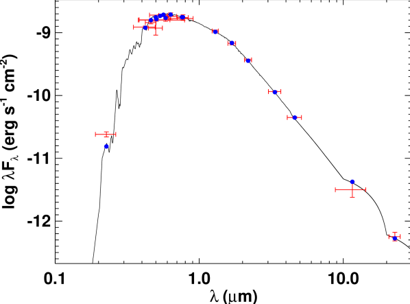
Figure 4: Spectral energy distribution of HD 110113. Red symbols represent the observed photometric measurements, where the horizontal bars represent the effective width of the passband. Blue symbols are the model fluxes from the best-fit Kurucz atmosphere model (black).

We performed a fit using Kurucz stellar atmosphere models, with the $T_{\rm eff}$, [Fe/H] and $\log g$ adopted from the spectroscopic analysis. The only additional free parameter is the extinction ($A_{V}$), which we restricted to the maximum line-of-sight value from the dust maps of Schlegel et al. (1998). The resulting fit is very good (Figure 4) with a reduced $\chi^{2}$ of 1.4 and best-fit $A_{V}=0.03\pm 0.03$. Integrating the (unreddened) model SED gives the bolometric flux at Earth, $F_{\rm bol}=2.597\pm 0.091\times 10^{-9}$ erg s^-1 cm^-2. Taking the $F_{\rm bol}$ and $T_{\rm eff}$ together with the Gaia DR2 parallax gives the stellar radius, $R_{\star}=0.968\pm 0.018R_{\odot}$. In addition, we can use the $R_{\star}$ together with the spectroscopic $\log g$ to obtain an empirical mass estimate of $M_{\star}=0.99\pm 0.08M_{\odot}$.

Taken together, all the stellar parameters as derived above are consistent, and all suggest that HD 110113 is a solar analogue with mass and radius very close to the Sun. As the SED radius measurement is least affected by sample size or systematic uncertainty, we assume this as a final radius. Similarly, the mass obtained from the $\log g$ and the SED-derived $R_{\star}$ ($0.99\pm 0.08M_{\odot}$) is nearly identical to that from the MR relationship ( $0.989\pm 0.01$  $M_{\odot}$), suggesting they converge on the same value. We therefore use the mass as defined from the offset-corrected Torres et al. (2010) calibrations, with the uncertainty inflated to reflect the typical systematic error ($0.06M_{\odot}$).

To compute the $v\sin{i}$ from the FWHM, we used the relations of Dos Santos et al. (2016), who studied the HARPS spectra of a large number of solar twins. We used this to first estimate the $v_{\rm macro}$ from the $T_{\rm eff}$ and $\log g$ derived in section 3.1.1 ($3.64\pm 0.1$ km s^-1), and then combined this with the measured FWHM to estimate a $v\sin{i}$ of $1.74\pm 0.15$ km s^-1, although the uncertainties here may be underestimated due to systematic uncertainties. Using the calculated $R_{s}$, this corresponds to a maximum rotation period ($P_{\rm max}$) of $28\pm 3$ d, assuming an aligned system.

3.1.2 Chemical abundances

Stellar abundances of the elements were also derived using the same tools and models as for stellar parameter determination as well as using the classical curve-of-growth analysis method assuming local thermodynamic equilibrium. Although the EWs of the spectral lines were automatically measured with ARES, for the elements with only two to three lines available we performed careful visual inspection of the EWs measurements. For the derivation of chemical abundances of refractory elements, we closely followed the methods described in the literature (e.g. Adibekyan et al., 2012; Adibekyan et al., 2015; Delgado Mena et al., 2014; Delgado Mena et al., 2017). Abundances of the volatile elements, O and C, were derived following the method of Delgado Mena et al. (2010); Bertran de Lis et al. (2015a). Since the two spectral lines of oxygen are usually weak and the 6300.3 Å line is blended with Ni and CN lines, the EWs of these lines were manually measured with the task splot in IRAF. Lithium and sulfur abundances were derived by performing spectral synthesis with MOOG, following the works by Delgado Mena et al. (2014) and Costa Silva et al. (2020) respectively. Both abundance indicators are very similar to the solar values. All the [X/H] ratios are obtained by doing a differential analysis with respect to a high S/N solar (Vesta) spectrum from HARPS. The stellar parameters and abundances of the elements are presented in Table 2.

We find that the [X/Fe] ratios of most elements are close to solar as expected for a star with this metallicity whereas [O/Fe] and [C/Fe] are slightly subsolar, since these ratios tend to slightly decrease above solar metallicity (e.g. Bertran de Lis et al., 2015b; Franchini et al., 2020). Moreover, we used the chemical abundances of some elements to derive ages through the so-called chemical clocks (i.e. certain chemical abundance ratios which have a strong correlation with age). We applied the 3D formulas described in Delgado Mena et al. (2019), which also consider the variation in age produced by the effective temperature and iron abundance. The chemical clocks [Y/Mg], [Y/Zn], [Y/Ti], [Y/Si], and [Y/Al] were derived. We selected the [Y/Al] age, 4.0 $\pm$ 0.5 Gyr, as the representative age, as it is consistent with all others and has the smallest uncertainty.

Parameter	Value	Error
Abundances
A(Li)	$1.09$	$0.08$
$[\rm{Fe}/\rm{H}]$	$0.14$	$0.02$
$[\rm{S}/\rm{H}]$	$0.03$	$0.04$
$[\rm{Na}/\rm{H}]$	$0.141$	$0.038$
$[\rm{Mg}/\rm{H}]$	$0.129$	$0.021$
$[\rm{Al}/\rm{H}]$	$0.105$	$0.014$
$[\rm{Si}/\rm{H}]$	$0.097$	$0.022$
$[\rm{Ca}/\rm{H}]$	$0.092$	$0.062$
$[\rm{Ti}/\rm{H}]$	$0.140$	$0.030$
$[\rm{Cr}/\rm{H}]$	$0.156$	$0.032$
$[\rm{Ni}/\rm{H}]$	$0.130$	$0.024$
$[\rm{O}/\rm{H}]$	$-0.012$	$0.083$
$[\rm{C}/\rm{H}]$	$0.032$	$0.012$
$[\rm{Cu}/\rm{H}]$	$0.116$	$0.016$
$[\rm{Zn}/\rm{H}]$	$0.050$	$0.012$
$[\rm{Sr}/\rm{H}]$	$0.170$	$0.073$
$[\rm{Y}/\rm{H}]$	$0.170$	$0.039$
$[\rm{Zr}/\rm{H}]$	$0.152$	$0.045$
$[\rm{Ba}/\rm{H}]$	$0.123$	$0.047$
$[\rm{Ce}/\rm{H}]$	$0.120$	$0.051$
$[\rm{Nd}/\rm{H}]$	$0.135$	$0.056$
Derived Abundance Ratios
Mg/Si	$1.32$	$0.09$
Fe/Si	$1.08$	$0.07$
Mg/Fe	$1.23$	$0.08$
Ages
$[\rm{Y}/\rm{Mg}]$ Age [Gyr]	$4.09$	$0.75$
$[\rm{Y}/\rm{Ti}]$ Age [Gyr]	$4.09$	$0.95$
$[\rm{Y}/\rm{Zn}]$ Age [Gyr]	$3.29$	$0.77$
$[\rm{Y}/\rm{Si}]$ Age [Gyr]	$3.95$	$0.86$
$[\rm{Y}/\rm{Al}]$ Age [Gyr]	$4.00$	$0.54$

Table 2: Derived stellar abundances. [Y/X] based ages using the 3D formula of Delgado Mena et al. (2019) (Table 10: age & $a+b\times$$T_{\rm eff}$$+c\times$$\rm[Fe/H]$$+d\times$$\rm[Y/Mg]$).

3.2 Combined modelling of RV & Photometry

3.2.1 Treatment of Radial Velocities

All activity indicators showed clear signs of stellar variability, likely due to the presence of starspots. To remove this stellar activity, we first turned to linear decorrelation of the RV signal using activity indicators. The FWHM and S-index showed the clearest rotational signals, so we selected these and used the decorrelation technique provided with the DACE spectroscopy Python package (Buchschacher et al., 2015). Despite this decorrelation removing much of the stellar variability signal, the peak at $\sim 22$d remained the single strongest signal in the radial velocity time series (see Figure 5). To remove the rotation signal at $23.68\pm 0.08$ d, we fitted a 5-parameter Keplerian model (with eccentricity $e$, argument of periastron $\Omega$, & semi-amplitude $K$ as free parameters, with period $P$ and time of transit $t_{0}$ constrained from the periodogram). The next strongest signals were at $6.73\pm 0.03$ d and $2.541\pm 0.0008$ d with amplitudes of $3.88\pm 0.31$ m s^-1 and $2.55\pm 0.31$ m s^-1 respectively. This was followed by signals on longer periods, which are most likely spurious due to rotational and observational aliases.

Although this linear decorrelation and Keplerian-fitted rotation period was able to reveal the planetary RV signals, stellar variability cannot in general be modelled as a Keplerian. Instead we turned to a Gaussian process (GP) to model the impact of rotation on the RVs. GPs have frequently been used in the analysis of radial velocities affected by activity (e.g. Haywood et al., 2014; Dumusque et al., 2019). One GP kernel well-suited to stellar rotation is a mix of simple harmonic oscillator (SHO) terms corresponding to $P_{\rm rot}$ and $P_{\rm rot}/2$, which we built using exoplanet and celerite packages.

In order to limit the impact of the GP on the planetary RV signal, we fitted activity indicators and RV time-series simultaneously with the same GP kernel, as these should follow the same underlying variations with the exception of planetary reflex motion. A similar approach was previously used by Grunblatt et al. (2015) to model stellar variability in the Kepler-78b system, and by Suárez Mascareño et al. (2020) to find an outer candidate orbiting Proxima Centauri. By explicitly linking the variation found across activity indicators and RVs, this method has the same effect as "training" a GP on an activity indicator (e.g. Dumusque et al., 2019). However, it avoids having to run multiple models consecutively and transfer the output PDF of a training sample into a second model—a process which loses information intrinsic to the likely non-Gaussian distributions of the GP hyper-parameters as well as information about the correlations between parameters. This technique also enables the use of multiple time-series. In this case, we chose S-index and FWHM to co-fit the covariance function with the RVs, as these showed the clearest rotation signal.

To achieve this, the hyper-parameters for rotation period, mix factor between $P_{\rm rot}$ and $P_{\rm rot}/2$ terms, signal quality ($Q$), and the difference in signal quality between modes ($\Delta Q$) were kept constant between S-index, FWHM and RV time-series, while the signal amplitude and mean, which are not shared across parameters, were set as separate parameters. For each time-series we also used a jitter term to model noise not included by measurement errors and to prevent GP over-fitting. All hyper-parameters were given broad priors, although the rotation period was constrained to the value obtained from a Lomb-Scargle periodogram (Lomb, 1976; Scargle, 1982) with a standard deviation of 20%. All parameter priors are listed in Table 5.

We also noted that the FWHM errors produced by the HARPS pipeline appeared over-estimated—more than twice the estimated error derived from the median absolute difference between measurements. Therefore the FWHM errors were multiplied by a factor of 0.4386 such that the median error matched the point-to-point RMS as calculated from the median absolute difference.

While we used the GPs to model the covariance between points in each timeseries, a mean function is also required to calibrate the average value over time, which we applied separately to each of the three timeseries. A 2-parameter (i.e. linear) trend term was included to model potential long-term drift in the RVs, although the resulting gradient was not significant ($-0.14\pm 0.73$ m s^-1d^-1). Single-parameter mean values were included to model the offset of S-index and FWHM from zero.

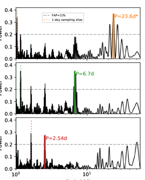
Figure 5: Periodograms of RVs after linear decorrelation with S-index and FWHM. The upper panel shows the raw periodogram, while subsequent panels show the periodogram after the removal of the previously marked peak. The 2.54 d peak is accompanied by a significant peak at the 1-day sampling alias (1.65 d), but the knowledge of a 2.54 d planet in the TESS photometry breaks this degeneracy. The remaining peaks in the final periodogram are likely due to sampling aliases associated with the $\sim 60$ d span of observations.

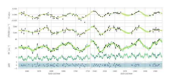
Figure 6: S-index, FWHM and RV timeseries of HD110113 for two seasons of HARPS monitoring, with GP models and 2-sigma uncertainty regions overplotted in green. Below the raw RV timeseries is the GP-removed RV timeseries, with the modelled planetary reflex motion and background trend (turquoise). At the very bottom the full model residuals are shown, with an RMS of only 1.31 m s^-1—extremely close to the median HARPS measurement uncertainty (1.36 m s^-1).

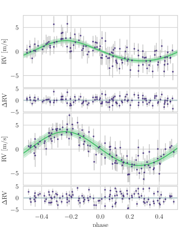
Figure 7: Phase-folded RVs (with the best-fit GP model, linear trend, and the other planetary signal removed) for HD 110113 b (top) and HD 110113 c (bottom), with model-subtracted residuals.

3.2.2 Treatment of Photometry

We downloaded the PDC_SAP lightcurve from the Mikulski Archive for Space Telescopes (MAST). As high-resolution imaging revealed no close stellar neighbours missed by e.g. the TESS input catalogue (Stassun et al., 2019), we made the assumption that the PDC-extracted and dilution-corrected lightcurve for this target was accurate.

We then normalised the PDC_SAP timeseries by its median and masked anomalous flux points from the timeseries by cutting data more than $4.2\sigma$ different from both preceding and succeeding neighbours.

We initially tried to use the same celerite GP kernel to predict both RV and photometric time-series deviations. This proved to not be possible, likely because the effect of stellar variability on photometry is not necessarily at the same timescale as for RVs (Aigrain et al., 2012). Similarly, although a Lomb-Scargle periodogram of the raw TESS lightcurve does show a peak with a period around 25d, the processed PDC_SAP lightcurve is flat, likely as variability on the order of a TESS orbit ($\sim 14$ d) is removed during processing.

The remaining variability is therefore likely to be the result of stellar granulation, which is well-suited to be modelled with a single GP SHO kernel with quality $Q=1/\sqrt{2}$ (Barros et al., 2020; Foreman-Mackey et al., 2017). To produce the initial hyperparameters ($\omega_{0}$ & $S_{0}$) and priors for the combined analysis and reduce the possibility of the GPs attempting to model the transits themselves, we first fitted this GP to the photometry with planetary transits cut. The interpolated posterior distributions from this analysis then provided the priors for the combined analysis. A jitter term was also included to model the effect of high-frequency noise not fully encapsulated by the photon noise (e.g. stellar & spacecraft jitter).

We modelled the limb darkening using two approaches: one where limb darkening is a free parameter, reparameterised using the approach of Kipping (2013b) and fitted to the transit with uninformative priors that cover the physical parameter space; and another where the expected theoretical limb darkening parameters for the star as generated by Claret (2017) are used as priors for the analysis. We found the resulting distributions to be consistent, and chose to use the second, constrained approach in the final modelling. This used a normal prior with the mean, $\mu$, set from the theoretical parameter and $\sigma$ set as 0.1 which we chose instead of the uncertainty found when propagating the stellar parameters through the Claret (2017) relation, which was likely too contsraining and did not account for systematic uncertainties. The radius ratio $R_{p}/R_{s}$ was treated using the log amplitude to avoid negative values, and b was reparameterised with $R_{p}/R_{s}$ following the exoplanet implementation of Espinoza (2018).

As ground-based photometry was not precise enough to observe a transit (see Sect. 2.2), we restrict this analysis to only the TESS photometry and HARPS spectroscopy.

3.2.3 Combined Model

We modelled full Keplerian orbits for the two planets, with eccentricity priors according to the Kipping (2013a) beta distribution.

Monte Carlo sampling, while able to explore the parameter space around a best-fit solution, does not deal well with exploring unconstrained parameters with multiple local minima. Therefore, in order to allow our model to explore a single solution, we included normal priors on period and $t_{0}$ using the values and uncertainties from the TOI catalogue in the case of the $2.54$d planet, and from the RV periodogram in the case of the $6.7$d planet. In all cases, we artificially inflated these uncertainties to make sure the parameters were not over-constrained by their priors, which is confirmed by noting that the posterior distributions are, in all cases, narrower than the priors.

The combined model, built using the exoplanet (Foreman-Mackey et al., 2020) package, was sampled using the No-U Turn Sampler (NUTS) in the Hamiltonian Monte Carlo PyMC back-end (Salvatier et al., 2016) using 5 independent chains with 2000 steps and an additional 500 steps burn-in. This produced 10000 independent samples. Model priors and posteriors are displayed in table 5.

The results from the combined model are shown in tables 3 and 5, with the HARPS RV timeseries and best-fit models shown in figure 6, phase-folded RVs and model shown in figure 7, and TESS photometry and best-fit light curves shown in figure 8.

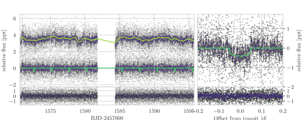
Figure 8: TESS photometry, where black dots represent individual 2-minute cadence data and dark circles (with errorbars) represent 30-minute bins. Upper left: TESS PDC_SAP time series with best-fit GP model (both offset by 3.5ppt), and GP-subtracted lightcurve with the best-fit transit model over-plotted (no offset). Lower left: residuals, with both GP model and transit models subtracted from the lightcurve. Upper right: phase-folded lightcurve of HD 110113 b zoomed to the transit. Lower right: phase-folded residuals.

Parameter	HD 110113 b	HD 110113 c
Epoch, $t_{0}$ [BJD-2457000]	$1570.101^{+0.004}_{-0.005}$	$1798.17\pm 0.19$
Orbital Period, $P$ [d]	$2.541^{+0.0005}_{-0.001}$	$6.744^{+0.008}_{-0.009}$
Semi-major Axis, $a$ [AU]	$0.035\pm 0.001$	$0.068^{+0.001}_{-0.002}$
Orbital Eccentricity, $e$	$0.093^{+0.079}_{-0.064}$	$0.045^{+0.079}_{-0.038}$
Argument of periastron, $\Omega$	$-0.47\pm 0.68$	$-0.1\pm 1.2$
Radius ratio [$R_{p}/R_{s}$]	$0.018\pm 0.001$	—
Radius, $R_{p}$ [$R_{\oplus}$]	$2.05\pm 0.12$	—
Impact Parameter, b	$0.31\pm 0.22$	—
Transit duration, $t_{D}$ [d]	$0.099^{+0.005}_{-0.007}$	—
RV semi-amplitude, $K$ [m s-1]	$2.15\pm 0.28$	$3.58\pm 0.37$
Planet Mass, $M_{p}$ [$M_{\oplus}$]	$4.55\pm 0.62$	$10.5\pm 1.2$ ⋆
Planet Density, $\rho_{p}$ [${\rm gcm}^{-3}$]	$2.90^{+0.75}_{-0.59}$	—
Insolation, $S$ [${\rm kWm}^{-2}$]	$1001.0\pm 40.0$	$272.0\pm 11.0$
Surface Temperature, $T_{p}$ [K]†	$1371.0\pm 14.0$	$990.0\pm 10.0$

Table 3: Derived planet properties. ^⋆ The mass of planet c refers to the $M_{p}\sin{i}$. ^† Surface temperature assumes a uniform surface and an albedo of 0.2.

4 Discussion

4.1 Evidence for HD 110113 c

The periodogram of the activity-corrected radial velocity timeseries showed a clear signal at $6.75$ d, even stronger than that of the planet at $2.54$ d (Figure 5). No such signal was found by TESS’ automatic TPS; however, there is a chance such a signal may have been missed. A search using the transit least squares algorithm (Hippke & Heller, 2019) on the HD 110113 b-subtracted lightcurve found no signal around 6.7 d, and a visual inspection of the lightcurve around the likely epochs of transits (given the limits from the RV detection) reveals no candidate dips associated with an outer candidate. Indeed, when running a combined model of two transiting planets, with constraints on orbits from the RVs, the posteriors for the radius of the outer planet were $<0.64$ R_⊕ at $1-\sigma$ which, given the $10.5\pm 1.2$  M_⊕ mass of HD 110113 c, would be physically impossible, even with an iron-core. Therefore, we come to the conclusion that HD 110113 c is likely non-transiting.

In order to assess whether the RV signal alone warrants calling HD 110113 c a confirmed planet or merely a candidate, we ran two combined models with identical priors and with one model including a non-transiting planet around $6.7$d. We then burned-in each model for 500 samples and ran the find_MAP function in PyMC3 to find the maximum likelihood for each model, allowing us to compare the difference in Bayesian Information Criterion ($\Delta{\rm BIC}$) between the models. The resulting value of $\Delta{\rm BIC}=$ $16.32$ clearly favours a two-planet model over a single planet model, with $\Delta{\rm BIC}>10$ suggesting "Very Strong" evidence over the null hypothesis.

Another test for the RV signal of HD 110113 c is the coherence of the signal over time, as radial velocity variation due to, e.g., stellar variability is not likely to remain coherent over multiple observing seasons. We verified this two ways using the decorrelated and rotation-subtracted radial velocities previously used to form RV periodograms (see Figure 5). First we processed each season individually, finding that the signals at 2.451 d and 6.75 d coincide with peaks during both seasons, albeit at lower signal strength. Next we applied the Bayesian generalised Lomb-Scargle periodogram (BGLS, Mortier et al., 2015) to subsets of our RV time series to test signal coherence as per the technique of Mortier & Collier Cameron (2017). Figure 9 shows that the signal of HD 110113 c passes this test - remaining evident even in datasets with only a handful of datapoints.

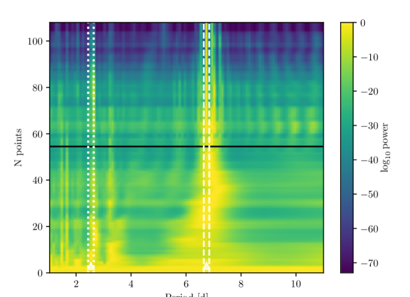
Figure 9: A 2D BGLS periodogram of HD 110113 radial velocities (after decorrelation and subtraction of the strongest rotation signal) performed on increasing numbers of radial velocity points, as proposed by Mortier & Collier Cameron (2017). Periods which maintain signal-strength and periodicity as a function of observation number suggest coherent (and therefore planetary) signals. The two white vertical bands show our modelled periods of each planet. The vertical bands seen are due to signal aliases in the second observing season due to the data gap, which is marked with a black horizontal line.

It should be noted that the period of HD 110113 c, at $6.744^{+0.008}_{-0.009}$  d, is close to the $P_{\rm rot}/3$ harmonic. However, there appears little evidence of a signal in the RV periodogram at $P_{\rm rot}/2$, so a large coherent signal at $P_{\rm rot}/3$ would be unexpected. However, it is possible that with certain inclinations and spot locations such harmonics may be boosted (Vanderburg et al., 2016; Boisse et al., 2011). Interestingly the periodogram of the S-index data does show a strong peak at $P_{\rm rot}/2$ and a weaker peak at $P_{\rm rot}/3$, but this occurs at $7.25$ d—significantly separated from the RV peak at $6.744^{+0.008}_{-0.009}$ . While we confirm the presence of this second planet, as given $\Delta{\rm BIC}>10$, the amplitude of the signal may be affected by the presence of a signal at $P_{\rm rot}/3$, therefore the mass of HD 110113 c should be treated as uncertain.

Multiple lines of evidence point to the signal of HD 110113 c being planetary in origin. Future RV measurements should help further disentangle stellar rotation and the signal amplitude, and may even reveal new candidates in this system.

The majority of short-period multi-planet systems are typically aligned with mutual inclinations of only a few degrees (Lissauer et al., 2011; Figueira et al., 2012; Winn & Fabrycky, 2015). To investigate whether this could also be true for HD 110113, we used the derived impact parameter of planet b and the semi-major axis ratio of b & c to calculate the expected impact parameter of planet c in a perfectly co-planar scenario ($b_{c}=0.60\pm 0.42$) and the minimum mutual inclination ($\Delta{}i=1.6^{+1.4\circ}_{-1.6}$). Therefore, the HD 110113 planetary system is still consistent with an aligned planetary system.

Throughout this work we quote $M_{p}\sin{i}$ for HD 110113 c. However, a clear non-detection of transits can constrain a planet’s inclination, and therefore also reduce the lower limit on a planet’s mass. However, in this case, the reduction in minimum mass caused by assuming $b>1.0$ is smaller than 0.25%. Therefore, including this factor would not significantly change the mass estimate from $M_{p}\sin{i}$. It is also worth noting that planets b & c have an orbital period ratio near 8/3, although harmonics beyond $2:1$ are highly unlikely to create measurable TTVs (Deck & Agol, 2015).

4.2 A solar analogue?

It is remarkable to note just how sun-like HD 110113 is, with a radius, $T_{\rm eff}$ and $\log g$ all within 1-sigma uncertainties of solar values, with the exception of its slightly higher metallicity ($\rm[Fe/H]$$=0.14\pm 0.02$), and correspondingly lower C & O (see Table 2) (e.g. Franchini et al., 2020; Bertran de Lis et al., 2015a). We speculate that the higher metallicity may explain why HD 110113 was able to form close-in mini-Neptunes (Mulders et al., 2016; Bitsch & Battistini, 2020), which do not exist in our solar system.

HD 110113 is also nearly the same age as the Sun, as can be seen in both the Yttrium-based ages (Table 2), and from the rotation rate ($\sim$22 d from archival photometry, spectroscopy timeseries, & $v\sin{i}$). Indeed, this rotation rate is marginally faster than the Sun (25–26.5 d when measured with HARPS-N and converted to sidereal period, Milbourne et al., 2019). This could be explained by the fact that HD 110113 is slightly younger, the Sun rotates slower than average (Robles et al., 2008), or the presence of short-period planets has tidally inhibited the slow-down of HD 110113, although the effect for such small planets is likely to be small (Bolmont et al., 2012).

Thanks to their similarities, HD 110113 and its planets could prove a useful comparison to the Sun and the solar system in the future.

4.3 Composition

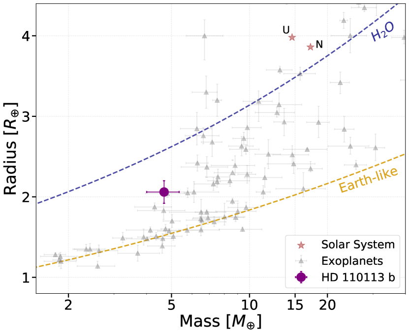
Figure 10: Mass-radius diagram of exoplanets with accurate mass and radius determination (Otegi et al. 2019). Also shown are the mass-radius relations for Earth-like and pure water compositions.

To explore the composition of HD 110113 b, we performed 4-layer interior structure modelling, using as inputs the mass and radius determined by our joint modelling of TESS photometry and HARPS RVs. We followed the method of Otegi et al. (2020), which assumes a pure iron core, a silicate mantle, a non-gaseous water layer, and a H-He atmosphere. In order to quantify the degeneracy between the different interior parameters and produce posterior probability distributions, we use a generalized Bayesian inference analysis with a Nested Sampling scheme (e.g. Buchner et al., 2014). The interior parameters that are inferred include the masses of the pure-iron core, silicate mantle, water layer and H-He atmosphere. The ratios of Fe/Si and Mg/Si found in stars is expected to be mirrored in the protoplanetary material, and therefore in the internal structures of exoplanets (Dorn et al., 2015). Hence, we use the values found by our stellar abundance analysis as a proxy for the core-to-mantle ratio. Given the observed molar ratio of Fe/Si ($1.08\pm 0.07$, Table 2) is higher than that of the Sun (0.85, Lodders et al., 2009), we would expect planetary material around HD 110113 to be more iron-rich than Earth.

Table 4 lists the inferred mass fractions of the core, mantle, water-layer and H-He atmosphere from the interior models. Due to the nature of the measurements, interior models cannot distinguish between water and H-He as the source of low-density material. Therefore, we ran both a 4-layer model and two 3-layer models, which leave out the H₂O and H-He envelopes, respectively. In the case of a H-He envelope, we find that the planet is only $\sim 1$% H-He by mass, with an iron-rich rocky interior making up 99% of the planet. Any water present would likely decrease the core, mantle & gaseous envelope fractions. However, a gas-free model would require $73^{+10}_{-13}$% water. Such a high water-to-rock ratio is challenging from formation point of view. Therefore HD 110113 b almost certainly has a significant gaseous envelope. Stars with super-solar metallicities are also less likely to host water-rich planets due to a higher C/O ratio (Bitsch & Battistini, 2020), making a water-rich composition even less likely.

Figure 10 shows the mass radius relation (M-R relation) for Earth-like and pure water compositions (where the pure water line corresponds to a surface pressure of 1 bar, and without a water-vapor atmosphere). Also shown are exoplanets with accurate mass and radius determinations from Otegi et al. (2020). The position of HD 110113 b makes it one of the lowest-density worlds found with $M_{p}<5$ M_⊕, and among a small class of low-density low-mass planets which includes $\pi{}$ Men c (Huang et al., 2018) and GJ 9827 b (Niraula et al., 2017).

Table 4: Inferred interior structure properties of TOI-755b.

Constituent	With H-He [%]	With H2O [%]	4-layer [%]
$M_{\rm core}/M_{\rm total}$	$47^{+26}_{-24}$	$8^{+7}_{-6}$	$25^{+28}_{-18}$
$M_{\rm mantle}/M_{\rm total}$	$53^{+23}_{-24}$	$17^{+11}_{-9}$	$36^{+31}_{-19}$
$M_{\rm water}/M_{\rm total}$	—	$73^{+10}_{-13}$	$38^{+31}_{-24}$
$M_{\rm H-He}/M_{\rm total}$	$1.0^{+0.3}_{-0.5}$	—	$0.102^{+0.04}_{-0.03}$

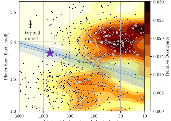
Figure 11: The distribution of Kepler planets by both insolation & planetary radius plot, with underlying occurrence distributions adapted from (Martinez et al., 2019). HD 110113 b is included as a purple star. The best-fit positions of radius valleys from both Martinez et al. (2019) (dashed) and Van Eylen et al. (2018) (dotted) are plotted in blue, with conversion from period to insolation performed using the average stellar parameters in the Kepler samples. Typical uncertainties for both HD 110113 c and for the Kepler sample are shown in the top left.

4.4 Evaporation

With an insolation of $1001.0\pm 40.0$  kW m^-2 ($\sim 736\,S_{\oplus}$), it is extremely likely that HD 110113 b has been moulded by strong stellar radiation in some way. This is further suggested by placing HD 110113 b on the insolation-radius plots of Fulton et al. (2017) and Martinez et al. (2019), which clearly show the "radius valley" (see Fig. 11. The negative slope of the valley with insolation means that, even with a radius of $2.05\pm 0.12$  R_⊕, HD 110113 b is positioned exactly within it.

Using both rotation and age, we predict a current X-ray luminosity ($L_{x}/L_{\rm bol}$) of between $8.5\times 10^{-7}$ (with Prot; Wright et al., 2018) and $2.74\times 10^{-6}$ (with age; Jackson et al., 2012). This implies total X-ray luminosities on the order of $3.3\times 10^{27}$ to $2.7\times 10^{28}$ erg and mass-loss rates (assuming an energy-limited regime) of between $5\times 10^{9}$ and $9\times 10^{9}$ gs^-1 (0.026– 0.05 $M_{\oplus}{\rm Gyr}^{-1}$). This is comparable to both GJ 436 b and Pi Men c under similar assumptions (King et al., 2019). Therefore, while it is currently highly irradiated, HD 110113 b is unlikely to currently be losing large quantities of its H-He atmosphere to space.

However, the integrated sum of mass-loss since the planet’s formation is substantial, as young stars are typically far more active and far more X-ray luminous. We calculate that, assuming the current mass and radius, as much as 10% of the planet’s mass may have been lost through evaporation. The models of Zeng et al. (2019) suggest that a 1000 K planet with $>5$% hydrogren and a $5.25M_{\oplus}$ core would have been $>8.5$ R_⊕ in radius, suggesting that HD 110113 b potentially started as an extremely low-density Jupiter-radius world which was quickly stripped. How such a low-mass world came to possess such a large gaseous atmosphere raises more questions.

In any case, it is highly likely that HD 110113 b started with a thicker atmosphere of H-He, which, due to both evaporative and core-powered mass-loss, it lost much of over time. However, this is typically a runaway process: planets which lose the majority of their gas (i.e. those in the radius valley) typically lose it all (Owen & Wu, 2017). Therefore the main unanswered question is: how did HD 110113 b escape becoming a naked core devoid of volatile envelope? Here we propose two solutions to this:

1) HD 110113 b started with a large envelope of H-He, perhaps as much as 10%, which was gradually lost to evaporation and core-powered heating over time. But it had just enough gas to walk the tight-rope between keeping hold of a thick atmosphere and being completely stripped such that, at the point that evaporative forcing stopped, HD 110113 b still had $\sim 1\%$ of H-He by mass. The models of Rogers & Owen (2020, Figure 4) suggest such a scenario is possible and may occur for planets that start gas-rich with around 4% H-He.

2) HD 110113 b did lose almost all of its H-He to evaporation and core-powered mass-loss. The current density is therefore explained by the planet having a large water content (e.g. an icy core), with potential out-gassing of a He-depleted secondary atmosphere contributing to the extended radius. Indeed, our composition calculations include water in only solid & liquid states; therefore a thick steam (or supercritical; Mousis et al., 2020) H₂O atmosphere could reduce the density without requiring $>50\%$ H₂O.

One final solution might be that HD 110113 b and HD 110113 c underwent late-stage migration to their current positions, thereby avoiding much of the evaporative forcing caused by the X-ray emissions of the young star. However, there is no theoretical mechanism in which a low-eccentricity 2-planet system could undergo such late-stage migration long after the dispersal of the protoplanetary disc. Instead, multi-planet systems are capabale of undergoing early-stage migration damped by the protoplanetary gas disc (Cresswell & Nelson, 2006; Carrera et al., 2019), and massive single planets are thought capable of undergoing late-stage, high-eccentricity scattering onto shorter orbits (Ford & Rasio, 2008; Beaugé & Nesvorný, 2012). We therefore consider a solution through in-situ processes more plausible than through migration.

These two predictions may be testable with future transmission spectroscopy observations, e.g. with JWST (Greene et al., 2016; Beichman et al., 2014).

4.5 Potential for future observations

The low-density nature of this hot mini-Neptune, combined with its bright host star, may enable transmission spectroscopy observations. Such measurement could test the hypotheses noted above, and search for a low-molecular weight primary atmosphere dominated by H-He, or a high molecular weight secondary atmosphere dominated by an overabundance of water vapour (Bean et al., 2020). To test this, we computed the emission and transmission spectroscopy metrics from Kempton et al. (2018).

We find that, amongst small planets with $R_{p}<4R_{\oplus}$ (Akeson et al., 2013), HD 110113 b ranks in the top 3% most amenable for emission and the top 5% for transmission spectroscopy with JWST. Although, when compared to one of the most favourable JWST targets: the low-density mini-Neptune GJ 1214 b, HD 110113 b provides only around 10% the SNR in both transmission & emission — as is expected when comparing with a planet whose transits are 36 times deeper.

HD 110113 b will be also re-observed by TESS during Sector 37, and could also be observed by ESA’s CHEOPS telescope (Benz et al., 2020), both of which would improve the radius precision below the currently measured value of 7%, thereby improving our knowledge of the internal structure of HD 110113 b.

5 Conclusion

We have presented the detection and confirmation of HD 110113 b, which was initially spotted as TOI-755.01 in TESS with an SNR of only $7.6\sigma$ and transit depth of 410 ppm. This marks one of the lowest-SNR signals yet to be confirmed from TESS, and is testament to the unique ability of TESS to find planet candidates around bright stars which can be redetected and characterised through independent RV campaigns.

High-resolution imaging and ground-based photometry rules out the presence of nearby companions and potential nearby eclipsing binaries, thereby limiting the number of false-positives and giving us confidence to follow such a low-SNR signal. Our subsequent HARPS campaign obtained more than 100 HARPS spectra in order to characterise both HD 110113 b and its bright ($G=9.9$ mag) star.

Analysis of these spectra revealed HD 110113 to be a Sun-like G-type star with slightly super-solar metallicity, but solar $T_{\rm eff}$, $\log g$ and age. The RV timeseries also revealed strong activity on HD 110113 with a rotation period of $20.8\pm 1.2$  d—a timescale corroborated by archival WASP photometry.

Removing this rotation period using both linear decorrelation and a co-fitted GP using S-index and FWHM activity indicators revealed the presence of two Keplerian signals, at $2.541^{+0.0005}_{-0.001}$  d and $6.744^{+0.008}_{-0.009}$  d. The inner signal, from a planet with mass $4.55\pm 0.62$  M_⊕, corresponded to the detected TESS candidate with a radius, as modelled from the TESS photometry, of $2.05\pm 0.12$  R_⊕. The outer signal, from a planet with $M_{p}\sin{i}$ of $10.5\pm 1.2$  M_⊕ did not correspond to any transit events in the TESS lightcurve, and therefore is likely non-transiting. We were able to confirm it as a planet through Bayesian model comparison which showed $\Delta{\rm BIC}=$$16.32$ in favour of a 2-planet model.

The estimated density of HD 110113 b is $2.90^{+0.75}_{-0.59}$  g cm^-3—far lower than would be expected from a rocky core. By modelling four potential constituents—an iron core, silicate mantle, water ocean and H-He atmosphere—we were able to rule out a gasless composition for HD 110113 b, suggesting that it has between 0.07 and 1.5% H-He by mass. This is surprising given HD 110113 b’s position in the "radius valley" between gaseous mini-Neptunes and rocky super-Earths, and we suggest two possibilities for this unexpectedly low density: either HD 110113 b has a water-rich core and secondary atmosphere, or it began with a thick H-He envelope and managed to retain a small fraction of it despite significant evaporation and/or heating. Follow-up spectroscopy observations with the next generation of telescopes may reveal the answer, as well as far more about this interesting system.

6 Data availability

The data underlying this article is publicly available - TESS data is stored on the Mikulski Archive for Space Telescopes (MAST) at https://archive.stsci.edu/tess/, while HARPS data is both available on the Data & Analysis Center for Exoplanets (DACE) at https://dace.unige.ch/, and in Appendix tables 6 & 7.

Appendix A Author Affiliations

¹ NCCR/PlanetS, Centre for Space & Habitability, University of Bern, Bern, Switzerland
² Department of Physics and Kavli Institute for Astrophysics and Space Research, Massachusetts Institute of Technology, Cambridge, MA 02139, USA
³ Centre for Exoplanets and Habitability, University of Warwick, Gibbet Hill Road, Coventry, CV4 7AL, UK
⁴ Department of Physics, University of Warwick, Gibbet Hill Road, Coventry CV4 7AL, UK
⁵ Instituto de Astrofísica e Ciências do Espaço, Universidade do Porto, CAUP, Rua das Estrelas, 4150-762 Porto, Portugal
⁶ Harvard-Smithsonian Center for Astrophysics, 60 Garden St, Cambridge, MA, 02138, USA
⁷ NASA Ames Research Center,Moffett Field, CA 94035, USA
⁸ Astrophysics Group, Keele University, Staffs ST5 5BG, U.K.
⁹ Centro de Astrobiologiía (CAB,CSIC-INTA), Dep. de Astrofísica, ESAC campus, 28692, Villanueva de la Cañada, Madrid, Spain
¹⁰ Geneva Observatory, University of Geneva, Chemin des Mailettes 51, 1290 Versoix, Switzerland
¹¹ Departamento de Física e Astronomia, Faculdade de Ciências, Universidade do Porto, Rua do Campo Alegre, 4169-007 Porto, Portugal
¹² Dunlap Institute for Astronomy and Astrophysics, University of Toronto, 50 St. George Street, Toronto, Ontario M5S 3H4, Canada
¹³ Cerro Tololo Inter-American Observatory, Casilla 603, La Serena, Chile
¹⁴ SETI Institute
¹⁵ American Association of Variable Star Observers, 49 Bay State Road, Cambridge, MA 02138, USA
¹⁶ International Center for Advanced Studies (ICAS) and ICIFI (CONICET), ECyT-UNSAM, Campus Miguelete, 25 de Mayo y Francia, (1650) Buenos Aires, Argentina.
¹⁷ Department of Physics and Astronomy, University of New Mexico, 1919 Lomas Blvd NE, Albuquerque, NM 87131, USA
¹⁸ Aix Marseille Univ, CNRS, CNES, LAM, Marseille, France
¹⁹ Institute for Computational Science, University of Zurich,Winterthurerstr. 190, CH-8057 Zurich, Switzerland
²⁰ Kavli Fellow
²¹ European Southern Observatory, Alonso de Cordova 3107, Vitacura, Santiago, Chile
²² Department of Physics & Astronomy, Swarthmore College, Swarthmore PA 19081, USA
²³ Department of Physics and Astronomy, The University of North Carolina at Chapel Hill, Chapel Hill, NC 27599-3255, USA
²⁴ Department of Astronomy, University of Maryland, College Park, MD 20742, USA
²⁵ Space Telescope Science Institute, 3700 San Martin Drive, Baltimore, MD 21218, USA
²⁶ Department of Earth, Atmospheric and Planetary Sciences, Massachusetts Institute of Technology, Cambridge, MA 02139, USA
²⁷ Department of Physics & Astronomy, Vanderbilt University, 6301 Stevenson Center Ln., Nashville, TN 37235, USA
²⁸ Department of Astrophysical Sciences, Princeton University, 4 Ivy Lane, Princeton, NJ 08544, USA

Appendix B Extra tables

Table 5: List of free parameters used in the exoplanet combined analysis of the TESS light curve and HARPS radial velocities with their associated prior and posterior distributions.

Parameter	Prior	Posterior
Stellar parameters
Stellar surface temperature, $T_{\rm eff}$ [K]	$\mathcal{N}(5732.0,50.0)$	$5732\pm 50$
Stellar Mass, $M_{s}$ [$M_{\odot}$]	$\mathcal{N}(0.9968,0.06)$	$0.997\pm 0.06$
Stellar Radius, $R_{s}$ [$R_{\odot}$]	$\mathcal{N}(0.968,0.018)$	$0.968\pm 0.018$
Orbital parameters
Transit Epoch, $t_{0}$ [BJD-2457000] b	$\mathcal{N}(1570.10189,0.1)$	$1570.101^{+0.004}_{-0.005}$
Transit Epoch, $t_{0}$ [BJD-2457000] c	$\mathcal{N}(1798.1334,1.0)$	$1798.17\pm 0.19$
Orbital Period, $P$ [d] b	$\mathcal{N}_{\mathcal{U}}(2.540455,0.002124,2.35,2.6)$	$2.541^{+0.0005}_{-0.001}$
Orbital Period, $P$ [d] c	$\mathcal{N}_{\mathcal{U}}(6.7285,0.05951,6.65,6.8)$	$6.744^{+0.008}_{-0.009}$
Orbital Eccentricity, $e$ b	$\beta(0.867;3.03)^{a}$	$0.093^{+0.079}_{-0.064}$
Orbital Eccentricity, $e$ c	$\beta(0.867;3.03)^{a}$	$0.045^{+0.079}_{-0.038}$
Argument of periastron, $\Omega$ b	$\mathcal{U}(-\pi,\pi)^{b}$	$-0.47\pm 0.68$
Argument of periastron, $\Omega$ c	$\mathcal{U}(-\pi,\pi)^{b}$	$-0.1\pm 1.2$
Photometric parameters
log radius ratio [$\log{R_{p}/R_{s}}$] b	$\mathcal{U}(-11.513,-2.3023)$	$-4.009\pm 0.063$
Transit Impact Parameter b	$\mathcal{U}(0,1+R_{p}/R_{s})^{c}$	$0.31\pm 0.22$
Quadratic Limb Darkening $a_{\rm LD}$	$\mathcal{N}_{\mathcal{U}}(0.367,0.1,0.0,1.0)$	$0.37\pm 0.1$
Quadratic Limb Darkening $b_{\rm LD}$	$\mathcal{N}_{\mathcal{U}}(0.21,0.1,0.0,1.0)$	$0.221^{+0.093}_{-0.096}$
Photometric jitter [$\log{\rm ppt}$]	$\mathcal{N}(0.7294,5.0)$	$-8.0^{+1.7}_{-2.6}$
Photometric GP power	$\mathcal{I}(0.014,0.006)^{d}$	$0.012\pm 0.003$
Photometric GP frequency [$d^{-1}$]	$\mathcal{I}(3.525,0.651)^{d}$	$3.73^{+0.48}_{-0.44}$
Photometric GP mean [ppt]	$\mathcal{I}(0.008,0.036)^{d}$	$0.011^{+0.031}_{-0.035}$
HARPS parameters
log RV semi-amplitude, $\log{K}$ b	$\mathcal{N}(0.3,5.0)$	$0.77\pm 0.13$
log RV semi-amplitude, $\log{K}$ c	$\mathcal{N}(0.3,5.0)$	$1.27\pm 0.1$
RV trend - intercept at BJD=2458779.717 [m s-1]	$\mathcal{N}(0.0,0.1)$	$0.027\pm 0.01$
RV trend - gradient [m s-1$d^{-1}$]	$\mathcal{N}(0.0,1.0)$	$-0.24\pm 0.7$
HARPS log jitter RV [m s-1]	$\mathcal{N}(1.992,5.0)$	$-0.5^{+0.7}_{-1.7}$
HARPS log jitter S index	$\mathcal{N}(6.527e-06,5.0)$	$-12.84^{+0.53}_{-0.74}$
HARPS log jitter FWHM [m s-1]	$\mathcal{N}(20.525,5.0)$	$0.1\pm 1.1$
HARPS mean S-index	$\mathcal{N}(0.0,0.00941)$	$-0.0^{+0.001}_{-0.002}$
HARPS mean FWHM [m s-1]	$\mathcal{N}(7287.75,7.5)$	$7286.9\pm 1.1$
HARPS GP log amplitude RV	$\mathcal{N}(2.984,8.0)$	$3.66^{+0.35}_{-0.34}$
HARPS GP log amplitude S-index	$\mathcal{N}(-9.332,8.0)$	$-9.64^{+0.37}_{-0.33}$
HARPS GP log amplitude FWHM	$\mathcal{N}(4.03,8.0)$	$3.77\pm 0.37$
HARPS GP log rotation period, $\log{P_{\rm rot}}/\log{d}$	$\mathcal{N}_{\mathcal{U}}(3.024,0.2,1.099,4.382)$	$3.035\pm 0.06$
HARPS GP log quality, $Q$	$\mathcal{N}(0.0,10.0)$	$-1.1^{+1.6}_{-3.6}$
HARPS GP log quality differential, $\Delta Q$	$\mathcal{N}(0.0,5.0)$	$1.7^{+1.8}_{-1.4}$
HARPS GP $P_{\rm rot}$ - $P_{\rm rot}/2$ mix factor	$\mathcal{U}(0,1)$	$20.8\pm 1.2$
$\mathcal{N}(\mu;\sigma^{2})$ is a normal distribution with mean $\mu$ and width $\sigma^{2}$, $\mathcal{U}(a;b)$ is a uniform distribution between $a$ and $b$, $\mathcal{N}_{\mathcal{U}}(\mu;\sigma^{2},a,b)$ is a normal distribution with mean $\mu$ and width $\sigma^{2}$ multiplied with a uniform distribution between $a$ and $b$, $\beta(a;b)$ is a Beta distribution with parameters $a$ and $b$, and $\mathcal{I}(\mu;\sigma^{2})$ is a distribution directly interpolated from the output of a pre-trained distribution with mean $\mu$ and standard deviation $\sigma^{2}$ (although the distribution may not follow a normal distribution). Posterior values and uncertainties represent the median and $1\sigma$ error boundaries. All other values (e.g. presented in Table 3) are directly determined from these fitted quantities. The prior uncertainties of input parameters $t_{0}$ and $P$ were inflated from the input data uncertainties by factors of: $t_{0,b}=23\times$, $t_{0,c}=7\times$, $P_{b}=3\times$, $P_{c}=11\times$. aDescribed in Kipping (2013a). bReparameterised in exoplanet to avoid discontinuities at $\pm\pi$. cexoplanet reparameterization of Espinoza (2018). dPyMc3 Interpolation function of pre-trained GP.

Table 6: HARPS spectroscopy from first season (June - August 2019)

Time	RV	$\sigma_{\rm RV}$	$S_{\rm MW}$	$\sigma_{S}$	FWHM	$\sigma_{\rm FWHM}$
$[\rm{BJD}-2457000]$	[m s-1]		–		[m s-1]
$1655.5493$	$1.8$	$1.95$	$0.0091$	$0.004$	$7281.8$	$4.5$
$1655.6181$	$1.32$	$2.0$	$0.0003$	$0.0045$	$7291.5$	$4.5$
$1656.6167$	$-4.08$	$2.39$	$0.0059$	$0.0064$	$7287.6$	$4.5$
$1657.5254$	$-6.07$	$1.44$	$0.0042$	$0.0025$	$7277.2$	$4.5$
$1657.606$	$-6.37$	$1.49$	$0.011$	$0.0029$	$7287.2$	$4.6$
$1658.5953$	$-3.78$	$1.46$	$-0.0045$	$0.0031$	$7292.7$	$4.6$
$1661.5662$	$0.04$	$1.48$	$-0.0048$	$0.003$	$7283.7$	$4.5$
$1664.5324$	$-13.5$	$1.36$	$-0.0074$	$0.0028$	$7280.8$	$4.5$
$1664.6282$	$-16.17$	$1.6$	$-0.0177$	$0.004$	$7276.6$	$4.5$
$1666.5674$	$-6.22$	$1.45$	$-0.0164$	$0.0029$	$7284.6$	$4.5$
$1667.5542$	$-8.01$	$1.39$	$-0.0127$	$0.0028$	$7285.4$	$4.6$
$1668.5189$	$3.21$	$1.8$	$-0.0126$	$0.0036$	$7284.8$	$4.5$
$1668.6197$	$5.3$	$1.88$	$-0.0178$	$0.0044$	$7289.2$	$4.5$
$1669.466$	$-3.47$	$1.32$	$-0.0046$	$0.0021$	$7276.4$	$4.5$
$1669.5709$	$-3.81$	$1.42$	$-0.015$	$0.0026$	$7277.4$	$4.5$
$1670.4637$	$-3.35$	$1.13$	$-0.0009$	$0.0015$	$7284.6$	$4.5$
$1670.5832$	$-3.13$	$1.46$	$-0.0052$	$0.0028$	$7293.5$	$4.6$
$1673.5985$	$2.86$	$1.53$	$0.0004$	$0.0032$	$7292.2$	$4.6$
$1674.5613$	$-0.04$	$1.69$	$-0.0008$	$0.0038$	$7296.6$	$4.6$
$1676.4716$	$2.3$	$1.62$	$0.0035$	$0.0034$	$7302.6$	$4.6$
$1676.5886$	$-2.22$	$1.88$	$-0.0014$	$0.0051$	$7297.6$	$4.6$
$1677.4681$	$-5.59$	$1.43$	$0.0078$	$0.0029$	$7294.7$	$4.6$
$1677.5491$	$-9.0$	$1.68$	$-0.0021$	$0.0043$	$7288.7$	$4.6$
$1679.5086$	$-12.66$	$1.12$	$-0.001$	$0.0019$	$7282.5$	$4.6$
$1679.571$	$-11.58$	$1.56$	$-0.0098$	$0.0036$	$7286.5$	$4.6$
$1680.5087$	$-10.82$	$1.09$	$-0.0003$	$0.0017$	$7280.1$	$4.6$
$1680.5634$	$-10.88$	$1.16$	$-0.0066$	$0.0021$	$7274.6$	$4.6$
$1681.5245$	$-4.52$	$1.54$	$-0.0098$	$0.0035$	$7277.2$	$4.5$
$1681.5771$	$-6.48$	$1.75$	$-0.0162$	$0.0043$	$7277.4$	$4.5$
$1682.4813$	$-5.11$	$1.23$	$-0.0081$	$0.002$	$7278.9$	$4.5$
$1682.5533$	$-9.81$	$1.35$	$-0.016$	$0.0028$	$7279.4$	$4.6$
$1684.5367$	$-7.71$	$1.75$	$-0.0143$	$0.0037$	$7282.2$	$4.5$
$1684.5971$	$-7.15$	$1.49$	$-0.0165$	$0.0031$	$7276.2$	$4.5$
$1685.4972$	$-3.64$	$1.39$	$-0.0081$	$0.003$	$7279.2$	$4.5$
$1685.5436$	$-7.43$	$1.69$	$-0.0174$	$0.0044$	$7281.9$	$4.6$
$1689.5056$	$6.68$	$1.47$	$-0.0023$	$0.0032$	$7287.8$	$4.6$
$1689.5493$	$5.35$	$1.83$	$-0.019$	$0.0047$	$7290.2$	$4.6$
$1690.4858$	$4.11$	$1.6$	$-0.0033$	$0.0032$	$7280.8$	$4.5$
$1691.5335$	$1.79$	$1.58$	$-0.005$	$0.0037$	$7287.9$	$4.6$
$1691.5549$	$1.87$	$1.62$	$-0.0057$	$0.0039$	$7283.2$	$4.6$
$1692.5178$	$4.23$	$1.59$	$-0.0053$	$0.0032$	$7294.8$	$4.5$
$1693.4664$	$7.52$	$1.36$	$0.002$	$0.0026$	$7291.0$	$4.5$
$1694.4709$	$8.59$	$1.19$	$0.0034$	$0.002$	$7288.2$	$4.5$
$1695.462$	$6.68$	$1.21$	$0.0056$	$0.0018$	$7287.3$	$4.5$
$1697.4761$	$0.74$	$2.07$	$-0.0023$	$0.0052$	$7288.8$	$4.5$
$1698.4702$	$-4.52$	$1.57$	$0.0019$	$0.0029$	$7288.1$	$4.5$
$1699.4797$	$-6.82$	$1.3$	$-0.0051$	$0.0024$	$7283.2$	$4.5$
$1700.4668$	$-7.25$	$1.29$	$0.0007$	$0.0023$	$7284.8$	$4.5$
$1701.4669$	$-2.83$	$1.19$	$-0.0044$	$0.0021$	$7272.8$	$4.5$
$1702.4715$	$-5.04$	$1.47$	$-0.0185$	$0.0032$	$7275.2$	$4.5$
$1703.4744$	$-13.62$	$1.76$	$-0.0192$	$0.0042$	$7269.0$	$4.5$
$1704.4713$	$-10.69$	$2.09$	$-0.024$	$0.0054$	$7274.8$	$4.5$
$1705.4964$	$-11.55$	$1.38$	$-0.0108$	$0.0029$	$7277.4$	$4.5$
$1706.4982$	$-8.22$	$1.47$	$-0.0119$	$0.0033$	$7279.4$	$4.5$
$1707.5135$	$-7.27$	$2.37$	$-0.0333$	$0.0066$	$7278.0$	$4.5$
$1708.4678$	$0.39$	$1.35$	$-0.0052$	$0.0026$	$7286.6$	$4.5$

Table 7: HARPS spectroscopy from second season (Dec 2019 - Feb 2020).

Time	RV	$\sigma_{\rm RV}$	$S_{\rm MW}$	$\sigma_{S}$	FWHM	$\sigma_{\rm FWHM}$
$[\rm{BJD}-2457000]$	[m s-1]		–		[m s-1]
$1838.8494$	$11.17$	$1.4$	$0.0147$	$0.0022$	$7301.0$	$4.5$
$1839.8578$	$6.52$	$1.26$	$0.0142$	$0.0017$	$7301.5$	$4.5$
$1840.8432$	$3.27$	$1.15$	$0.0136$	$0.0014$	$7294.8$	$4.5$
$1841.8384$	$3.16$	$1.19$	$0.0097$	$0.0015$	$7292.3$	$4.5$
$1842.8077$	$-3.96$	$1.45$	$0.0039$	$0.0022$	$7286.0$	$4.5$
$1843.8559$	$-2.03$	$1.74$	$-0.0018$	$0.0029$	$7284.0$	$4.5$
$1844.8362$	$-13.35$	$1.16$	$-0.0026$	$0.0014$	$7274.8$	$4.5$
$1845.8271$	$-12.38$	$1.33$	$-0.0073$	$0.002$	$7272.5$	$4.5$
$1847.8389$	$-14.59$	$1.11$	$-0.0095$	$0.0012$	$7274.5$	$4.5$
$1849.7822$	$-1.97$	$1.18$	$-0.0042$	$0.0015$	$7282.3$	$4.5$
$1849.8576$	$-3.28$	$1.13$	$-0.0055$	$0.0013$	$7282.4$	$4.5$
$1850.7988$	$0.75$	$1.08$	$0.0006$	$0.0013$	$7283.3$	$4.5$
$1850.8597$	$2.51$	$1.04$	$-0.001$	$0.0011$	$7285.2$	$4.5$
$1852.7908$	$-1.78$	$1.17$	$0.0036$	$0.0015$	$7289.0$	$4.5$
$1852.8609$	$-0.05$	$1.42$	$0.0059$	$0.0021$	$7287.6$	$4.5$
$1853.8015$	$1.87$	$1.25$	$0.0071$	$0.0017$	$7296.4$	$4.5$
$1853.8644$	$6.84$	$1.68$	$0.0055$	$0.003$	$7298.1$	$4.5$
$1854.757$	$4.48$	$1.88$	$-0.0022$	$0.0043$	$7301.3$	$4.5$
$1854.8269$	$-1.07$	$1.62$	$-0.0036$	$0.0031$	$7287.3$	$4.5$
$1855.8321$	$2.95$	$1.38$	$0.0034$	$0.0022$	$7291.6$	$4.5$
$1858.775$	$7.83$	$1.33$	$0.0067$	$0.002$	$7300.9$	$4.5$
$1858.8351$	$8.32$	$1.31$	$0.0079$	$0.0018$	$7296.7$	$4.5$
$1859.7796$	$5.81$	$1.44$	$0.0076$	$0.0024$	$7297.4$	$4.5$
$1860.7517$	$-2.5$	$1.26$	$0.008$	$0.0018$	$7289.7$	$4.5$
$1860.8525$	$-4.61$	$1.19$	$0.0083$	$0.0015$	$7290.3$	$4.5$
$1861.7734$	$2.82$	$1.22$	$0.0061$	$0.0016$	$7285.7$	$4.5$
$1861.85$	$3.7$	$1.22$	$0.0075$	$0.0015$	$7289.9$	$4.5$
$1862.7588$	$-0.94$	$1.1$	$0.0043$	$0.0012$	$7293.8$	$4.5$
$1862.8378$	$-0.75$	$1.19$	$0.0089$	$0.0014$	$7296.8$	$4.5$
$1863.7554$	$2.21$	$1.13$	$0.0048$	$0.0014$	$7294.8$	$4.5$
$1863.8328$	$1.3$	$1.06$	$0.0039$	$0.0011$	$7292.6$	$4.5$
$1864.7737$	$-0.21$	$1.25$	$0.0048$	$0.0017$	$7293.5$	$4.5$
$1864.8432$	$-3.66$	$1.46$	$0.005$	$0.0022$	$7296.3$	$4.5$
$1865.8255$	$-9.78$	$1.41$	$0.0104$	$0.002$	$7289.3$	$4.5$
$1876.7398$	$6.07$	$1.26$	$0.0029$	$0.0018$	$7281.5$	$4.5$
$1876.8589$	$7.09$	$1.32$	$-0.0009$	$0.0018$	$7277.0$	$4.5$
$1877.7559$	$4.9$	$1.25$	$0.0009$	$0.0017$	$7285.7$	$4.5$
$1879.7785$	$4.46$	$1.56$	$0.0045$	$0.0025$	$7290.9$	$4.5$
$1880.7355$	$4.05$	$1.22$	$0.0087$	$0.0016$	$7294.9$	$4.5$
$1880.8847$	$1.67$	$1.22$	$0.0083$	$0.0017$	$7296.2$	$4.5$
$1881.7267$	$10.47$	$1.23$	$0.0099$	$0.0016$	$7289.8$	$4.5$
$1882.8435$	$14.18$	$1.23$	$0.0126$	$0.0015$	$7295.8$	$4.5$
$1883.7334$	$14.27$	$1.17$	$0.0151$	$0.0015$	$7300.2$	$4.5$
$1883.8645$	$16.62$	$1.26$	$0.0136$	$0.0017$	$7302.6$	$4.5$
$1894.7258$	$-3.86$	$1.43$	$-0.0031$	$0.0021$	$7283.7$	$4.5$
$1894.859$	$-4.95$	$1.49$	$-0.0048$	$0.0022$	$7286.4$	$4.5$
$1897.8044$	$8.9$	$1.29$	$-0.0005$	$0.0017$	$7291.1$	$4.5$
$1897.8921$	$6.79$	$1.5$	$-0.0025$	$0.0026$	$7283.0$	$4.5$
$1898.8055$	$8.8$	$1.18$	$0.0065$	$0.0014$	$7290.6$	$4.5$
$1899.7514$	$10.63$	$1.17$	$0.0079$	$0.0015$	$7288.3$	$4.5$
$1899.8854$	$7.06$	$1.2$	$0.0057$	$0.0019$	$7291.0$	$4.5$
$1900.7715$	$3.46$	$1.11$	$0.0071$	$0.0013$	$7295.4$	$4.5$
$1900.8838$	$3.59$	$1.21$	$0.0054$	$0.002$	$7289.1$	$4.5$
$1901.7655$	$5.17$	$1.07$	$0.0084$	$0.0012$	$7289.1$	$4.5$
$1902.6953$	$12.1$	$1.13$	$0.0102$	$0.0014$	$7289.0$	$4.5$
$1902.8507$	$12.72$	$1.16$	$0.0106$	$0.0017$	$7291.3$	$4.5$
$1903.7072$	$14.72$	$1.07$	$0.011$	$0.0012$	$7285.1$	$4.5$
$1903.885$	$15.9$	$1.26$	$0.0071$	$0.0022$	$7290.0$	$4.5$

References

- Adibekyan et al. (2012) Adibekyan V. Z., Sousa S. G., Santos N. C., Delgado Mena E., González Hernández J. I., Israelian G., Mayor M., Khachatryan G., 2012, A&A, 545, A32
- Adibekyan et al. (2015) Adibekyan V., et al., 2015, A&A, 583, A94
- Agol et al. (2019) Agol E., Luger R., Foreman-Mackey D., 2019, arXiv e-prints
- Aigrain et al. (2012) Aigrain S., Pont F., Zucker S., 2012, Monthly Notices of the Royal Astronomical Society, 419, 3147
- Akeson et al. (2013) Akeson R., et al., 2013, Publications of the Astronomical Society of the Pacific, 125, 989
- Aller et al. (2020) Aller A., Lillo-Box J., Jones D., Miranda L. F., Barceló Forteza S., 2020, A&A, 635, A128
- Armstrong et al. (2020) Armstrong D. J., et al., 2020, Nature, 583, 39
- Astropy Collaboration et al. (2013) Astropy Collaboration et al., 2013, A&A, 558, A33
- Astropy Collaboration et al. (2018) Astropy Collaboration et al., 2018, AJ, 156, 123
- Baranne et al. (1996) Baranne A., et al., 1996, A&AS, 119, 373
- Barros et al. (2020) Barros S. C. C., Demangeon O., Díaz R. F., Cabrera J., Santos N. C., Faria J. P., Pereira F., 2020, A&A, 634, A75
- Bean et al. (2020) Bean J. L., Raymond S. N., Owen J. E., 2020, arXiv e-prints, p. arXiv:2010.11867
- Beaugé & Nesvorný (2012) Beaugé C., Nesvorný D., 2012, ApJ, 751, 119
- Beichman et al. (2014) Beichman C., et al., 2014, PASP, 126, 1134
- Benz et al. (2020) Benz W., et al., 2020, arXiv preprint arXiv:2009.11633
- Berger et al. (2020) Berger T. A., Huber D., van Saders J. L., Gaidos E., Tayar J., Kraus A. L., 2020, AJ, 159, 280
- Bertran de Lis et al. (2015b) Bertran de Lis S., Delgado Mena E., Adibekyan V. Z., Santos N. C., Sousa S. G., 2015b, A&A, 576, A89
- Bertran de Lis et al. (2015a) Bertran de Lis S., Delgado Mena E., Adibekyan V. Z., Santos N. C., Sousa S. G., 2015a, A&A, 576, A89
- Bitsch & Battistini (2020) Bitsch B., Battistini C., 2020, Astronomy & Astrophysics, 633, A10
- Boisse et al. (2009) Boisse I., et al., 2009, A&A, 495, 959
- Boisse et al. (2011) Boisse I., Bouchy F., Hébrard G., Bonfils X., Santos N., Vauclair S., 2011, Astronomy & Astrophysics, 528, A4
- Bolmont et al. (2012) Bolmont E., Raymond S. N., Leconte J., Matt S. P., 2012, Astronomy & Astrophysics, 544, A124
- Brown et al. (2013) Brown T. M., et al., 2013, Publications of the Astronomical Society of the Pacific, 125, 1031
- Brown et al. (2018) Brown A., et al., 2018, Astronomy & astrophysics, 616, A1
- Buchner et al. (2014) Buchner J., et al., 2014, A&A, 564, A125
- Buchschacher et al. (2015) Buchschacher N., Ségransan D., Udry S., Díaz R., 2015, in Taylor A. R., Rosolowsky E., eds, Astronomical Society of the Pacific Conference Series Vol. 495, Astronomical Data Analysis Software an Systems XXIV (ADASS XXIV). p. 7
- Carleo et al. (2020) Carleo I., et al., 2020, arXiv preprint arXiv:2004.10095
- Carrera et al. (2019) Carrera D., Ford E. B., Izidoro A., 2019, MNRAS, 486, 3874
- Choi et al. (2016) Choi J., Dotter A., Conroy C., Cantiello M., Paxton B., Johnson B. D., 2016, ApJ, 823, 102
- Claret (2017) Claret A., 2017, Astronomy & Astrophysics, 600, A30
- Cloutier et al. (2020) Cloutier R., et al., 2020, The Astronomical Journal, 160, 3
- Collins et al. (2017) Collins K. A., Kielkopf J. F., Stassun K. G., Hessman F. V., 2017, AJ, 153, 77
- Costa Silva et al. (2020) Costa Silva A. R., Delgado Mena E., Tsantaki M., 2020, A&A, 634, A136
- Cresswell & Nelson (2006) Cresswell P., Nelson R. P., 2006, A&A, 450, 833
- Deck & Agol (2015) Deck K. M., Agol E., 2015, The Astrophysical Journal, 802, 116
- Delgado Mena et al. (2010) Delgado Mena E., Israelian G., González Hernández J. I., Bond J. C., Santos N. C., Udry S., Mayor M., 2010, ApJ, 725, 2349
- Delgado Mena et al. (2014) Delgado Mena E., et al., 2014, A&A, 562, A92
- Delgado Mena et al. (2017) Delgado Mena E., Tsantaki M., Adibekyan V. Z., Sousa S. G., Santos N. C., González Hernández J. I., Israelian G., 2017, A&A, 606, A94
- Delgado Mena et al. (2019) Delgado Mena E., et al., 2019, A&A, 624, A78
- Dorn et al. (2015) Dorn C., Khan A., Heng K., Connolly J. A., Alibert Y., Benz W., Tackley P., 2015, Astronomy & Astrophysics, 577, A83
- Dos Santos et al. (2016) Dos Santos L. A., et al., 2016, Astronomy & Astrophysics, 592, A156
- Dumusque et al. (2019) Dumusque X., et al., 2019, A&A, 627, A43
- Espinoza (2018) Espinoza N., 2018, arXiv preprint arXiv:1811.04859
- Figueira et al. (2012) Figueira P., et al., 2012, A&A, 541, A139
- Ford & Rasio (2008) Ford E. B., Rasio F. A., 2008, ApJ, 686, 621
- Foreman-Mackey (2018) Foreman-Mackey D., 2018, Research Notes of the American Astronomical Society, 2, 31
- Foreman-Mackey et al. (2017) Foreman-Mackey D., Agol E., Ambikasaran S., Angus R., 2017, AJ, 154, 220
- Foreman-Mackey et al. (2020) Foreman-Mackey D., Luger R., Czekala I., Agol E., Price-Whelan A., Barclay T., 2020, exoplanet-dev/exoplanet v0.3.2, doi:10.5281/zenodo.1998447, https://doi.org/10.5281/zenodo.1998447
- Franchini et al. (2020) Franchini M., et al., 2020, ApJ, 888, 55
- Fulton et al. (2017) Fulton B. J., et al., 2017, The Astronomical Journal, 154, 109
- Ginzburg et al. (2018) Ginzburg S., Schlichting H. E., Sari R., 2018, Monthly Notices of the Royal Astronomical Society, 476, 759
- Gomes da Silva et al. (2011) Gomes da Silva J., Santos N. C., Bonfils X., Delfosse X., Forveille T., Udry S., 2011, A&A, 534, A30
- Greene et al. (2016) Greene T. P., Line M. R., Montero C., Fortney J. J., Lustig-Yaeger J., Luther K., 2016, ApJ, 817, 17
- Grunblatt et al. (2015) Grunblatt S. K., Howard A. W., Haywood R. D., 2015, The Astrophysical Journal, 808, 127
- Harris et al. (2020) Harris C. R., et al., 2020, Nature, 585, 357
- Haywood et al. (2014) Haywood R. D., et al., 2014, MNRAS, 443, 2517
- Henden et al. (2015) Henden A. A., Levine S., Terrell D., Welch D. L., 2015, in American Astronomical Society Meeting Abstracts #225. p. 336.16
- Hippke & Heller (2019) Hippke M., Heller R., 2019, Astronomy & Astrophysics, 623, A39
- Howell et al. (2011) Howell S. B., Everett M. E., Sherry W., Horch E., Ciardi D. R., 2011, AJ, 142, 19
- Huang et al. (2018) Huang C. X., et al., 2018, The Astrophysical Journal Letters, 868, L39
- Huber (2017) Huber D., 2017, Isoclassify: V1.2, doi:10.5281/zenodo.573372
- Hunter (2007) Hunter J. D., 2007, Computing in science & engineering, 9, 90
- Jackson et al. (2012) Jackson A. P., Davis T. A., Wheatley P. J., 2012, Monthly Notices of the Royal Astronomical Society, 422, 2024
- Jenkins et al. (2010) Jenkins J. M., et al., 2010, in Radziwill N. M., Bridger A., eds, Society of Photo-Optical Instrumentation Engineers (SPIE) Conference Series Vol. 7740, Software and Cyberinfrastructure for Astronomy. p. 77400D, doi:10.1117/12.856764
- Jenkins et al. (2016) Jenkins J. M., et al., 2016, in Software and Cyberinfrastructure for Astronomy IV. p. 99133E
- Jensen (2013) Jensen E., 2013, ascl, pp ascl–1306
- Kane et al. (2020) Kane S. R., et al., 2020, The Astronomical Journal, 160, 129
- Kempton et al. (2018) Kempton E. M.-R., et al., 2018, Publications of the Astronomical Society of the Pacific, 130, 114401
- King et al. (2019) King G. W., Wheatley P. J., Bourrier V., Ehrenreich D., 2019, Monthly Notices of the Royal Astronomical Society: Letters, 484, L49
- Kipping (2013a) Kipping D. M., 2013a, Monthly Notices of the Royal Astronomical Society: Letters, 434, L51
- Kipping (2013b) Kipping D. M., 2013b, Monthly Notices of the Royal Astronomical Society, 435, 2152
- Kurucz (1993) Kurucz R. L., 1993, SYNTHE spectrum synthesis programs and line data
- Li et al. (2019) Li J., Tenenbaum P., Twicken J. D., Burke C. J., Jenkins J. M., Quintana E. V., Rowe J. F., Seader S. E., 2019, PASP, 131, 024506
- Lissauer et al. (2011) Lissauer J. J., et al., 2011, The Astrophysical Journal Supplement Series, 197, 8
- Lodders et al. (2009) Lodders K., Palme H., Gail H.-P., 2009, in , Solar system. Springer, pp 712–770
- Lomb (1976) Lomb N. R., 1976, Ap&SS, 39, 447
- Luger et al. (2019) Luger R., Agol E., Foreman-Mackey D., Fleming D. P., Lustig-Yaeger J., Deitrick R., 2019, AJ, 157, 64
- Martinez et al. (2019) Martinez C. F., Cunha K., Ghezzi L., Smith V. V., 2019, The Astrophysical Journal, 875, 29
- Maxted et al. (2011) Maxted P. F. L., et al., 2011, PASP, 123, 547
- Mayor et al. (2003) Mayor M., et al., 2003, The Messenger, 114, 20
- McCully et al. (2018) McCully C., Volgenau N. H., Harbeck D.-R., Lister T. A., Saunders E. S., Turner M. L., Siiverd R. J., Bowman M., 2018, in Proc. SPIE. p. 107070K (arXiv:1811.04163), doi:10.1117/12.2314340
- McKinney et al. (2011) McKinney W., et al., 2011, Python for High Performance and Scientific Computing, 14
- Milbourne et al. (2019) Milbourne T., et al., 2019, The Astrophysical Journal, 874, 107
- Mortier & Collier Cameron (2017) Mortier A., Collier Cameron A., 2017, A&A, 601, A110
- Mortier et al. (2015) Mortier A., Faria J. P., Correia C. M., Santerne A., Santos N. C., 2015, A&A, 573, A101
- Mousis et al. (2020) Mousis O., Deleuil M., Aguichine A., Marcq E., Naar J., Aguirre L. A., Brugger B., Goncalves T., 2020, arXiv preprint arXiv:2002.05243
- Mulders et al. (2016) Mulders G. D., Pascucci I., Apai D., Frasca A., Molenda-Żakowicz J., 2016, The Astronomical Journal, 152, 187
- Nielsen et al. (2020) Nielsen L. D., et al., 2020, Monthly Notices of the Royal Astronomical Society, 492, 5399
- Niraula et al. (2017) Niraula P., et al., 2017, The Astronomical Journal, 154, 266
- Nowak et al. (2020) Nowak G., et al., 2020, arXiv preprint arXiv:2003.01140
- Onken et al. (2020) Onken C. A., et al., 2020, arXiv e-prints, p. arXiv:2008.10359
- Otegi et al. (2020) Otegi J., Bouchy F., Helled R., 2020, Astronomy & Astrophysics, 634, A43
- Owen & Wu (2017) Owen J. E., Wu Y., 2017, The Astrophysical Journal, 847, 29
- Pepe et al. (2002) Pepe F., et al., 2002, The Messenger, 110, 9
- Pollacco et al. (2006) Pollacco D. L., et al., 2006, PASP, 118, 1407
- Queloz et al. (2001) Queloz D., et al., 2001, A&A, 379, 279
- Quinn et al. (2019) Quinn S. N., et al., 2019, The Astronomical Journal, 158, 177
- Ricker et al. (2016) Ricker G. R., et al., 2016, in Space Telescopes and Instrumentation 2016: Optical, Infrared, and Millimeter Wave. p. 99042B
- Robitaille et al. (2013) Robitaille T. P., et al., 2013, Astronomy & Astrophysics, 558, A33
- Robles et al. (2008) Robles J. A., Lineweaver C. H., Grether D., Flynn C., Egan C. A., Pracy M. B., Holmberg J., Gardner E., 2008, ApJ, 684, 691
- Rogers & Owen (2020) Rogers J. G., Owen J. E., 2020, arXiv preprint arXiv:2007.11006
- Salvatier et al. (2016) Salvatier J., Wiecki T. V., Fonnesbeck C., 2016, PeerJ Computer Science, 2, e55
- Santos et al. (2013a) Santos N. C., et al., 2013a, A&A, 556, A150
- Santos et al. (2013b) Santos N. C., et al., 2013b, A&A, 556, A150
- Scargle (1982) Scargle J. D., 1982, ApJ, 263, 835
- Schlegel et al. (1998) Schlegel D. J., Finkbeiner D. P., Davis M., 1998, ApJ, 500, 525
- Skrutskie et al. (2006) Skrutskie M., et al., 2006, The Astronomical Journal, 131, 1163
- Smith et al. (2012) Smith J. C., et al., 2012, PASP, 124, 1000
- Sneden (1973) Sneden C., 1973, ApJ, 184, 839
- Sousa et al. (2008) Sousa S. G., et al., 2008, A&A, 487, 373
- Sousa et al. (2011) Sousa S. G., Santos N. C., Israelian G., Mayor M., Udry S., 2011, A&A, 533, A141
- Stassun & Torres (2016) Stassun K. G., Torres G., 2016, AJ, 152, 180
- Stassun & Torres (2018) Stassun K. G., Torres G., 2018, ApJ, 862, 61
- Stassun et al. (2017) Stassun K. G., Collins K. A., Gaudi B. S., 2017, AJ, 153, 136
- Stassun et al. (2018) Stassun K. G., Corsaro E., Pepper J. A., Gaudi B. S., 2018, AJ, 155, 22
- Stassun et al. (2019) Stassun K. G., et al., 2019, The Astronomical Journal, 158, 138
- Stumpe et al. (2012) Stumpe M. C., et al., 2012, Publications of the Astronomical Society of the Pacific, 124, 985
- Stumpe et al. (2014) Stumpe M. C., Smith J. C., Catanzarite J. H., Van Cleve J. E., Jenkins J. M., Twicken J. D., Girouard F. R., 2014, Publications of the Astronomical Society of the Pacific, 126, 100
- Suárez Mascareño et al. (2020) Suárez Mascareño A., et al., 2020, A&A, 639, A77
- Theano Development Team (2016) Theano Development Team 2016, arXiv e-prints, abs/1605.02688
- Tokovinin (2018) Tokovinin A., 2018, Publications of the Astronomical Society of the Pacific, 130, 035002
- Torres et al. (2010) Torres G., Andersen J., Giménez A., 2010, A&ARv, 18, 67
- Twicken et al. (2018) Twicken J. D., et al., 2018, PASP, 130, 064502
- Van Eylen et al. (2018) Van Eylen V., Agentoft C., Lundkvist M., Kjeldsen H., Owen J. E., Fulton B. J., Petigura E., Snellen I., 2018, Monthly Notices of the Royal Astronomical Society, 479, 4786
- Vanderburg et al. (2016) Vanderburg A., Plavchan P., Johnson J. A., Ciardi D. R., Swift J., Kane S. R., 2016, Monthly Notices of the Royal Astronomical Society, 459, 3565
- Virtanen et al. (2020) Virtanen P., et al., 2020, Nature methods, 17, 261
- Winn & Fabrycky (2015) Winn J. N., Fabrycky D. C., 2015, Annual Review of Astronomy and Astrophysics, 53
- Wright et al. (2018) Wright N. J., Newton E. R., Williams P. K., Drake J. J., Yadav R. K., 2018, Monthly Notices of the Royal Astronomical Society, 479, 2351
- Zeng et al. (2019) Zeng L., et al., 2019, Proceedings of the National Academy of Sciences, 116, 9723
- Ziegler et al. (2020) Ziegler C., Tokovinin A., Briceno C., Mang J., Law N., Mann A., 2020, yCat, pp J–AJ