TIT Yun Wei, Bala Rajaratnam and Alfred Hero
Duke University, University of California and University of Michigan
Email: cloudwei@umich.edu, brajaratnam@ucdavis.edu and hero@eecs.umich.edu

To: the Editors and Referees of the IEEE Transaction on Information Theory

Re: Revision of Manuscript ID IT-21-0152: A unified framework for correlation mining in ultra-high dimension

We are pleased to submit a revision of our manuscript to IEEE Transaction on Information Theory. We would like to sincerely thank the Editors and the Referees for your valuable suggestions and comments in the reviews.

For the benefit of the editor and the reviewers, we summarize the major changes, which are made in order to comprehensively address the comments of the reviewers. We believe that these changes significantly improve the paper. Among the principal changes are the following. Firstly we have added a subsection in the introduction that concisely summarizes our contributions and more clearly places them within the context of previous work. Secondly, since some reviewers found that the informal derivation to motivate Proposition LABEL:prop:edgecor in Section LABEL:sec:closenessnumedge was too technical, and disrupted the flow, we have moved it to Section LABEL:sec:derivationprop:edgecor in the Appendix. We have made a concerted effort to try and respond comprehensively to all comments of the reviewers and have made several improvements to the paper based on Referee feedback.

In what follows the Referee’s comments are in black, our responses are in blue and the changes we made to our paper are in red.

1 Responses to Associate Editor’s comments (from email)

1. Comment Specifically, while there are a number of technical points raised by the reviewers, one of the more substantial concerns raised by multiple reviewers concerns the novelty/significance of your work compared to some of the most closely related prior work. (I will also note that two of the reviewers raised concerns about the suitability of Transactions on Information Theory as an appropriate venue – while you should feel free to address this concern in your response, I will say that this is not an issue that I am worried about with this paper.)
   

   Response We thank the AE for giving us an opportunity to revise the paper and for his encouraging remarks, especially regarding the issue of the suitability of Transactions on Information Theory as an appropriate venue. Per your request, in this revision we have comprehensively addressed the technical points raised by the reviewers. This 20 page ”Response to reviewer document” attests to the sheer amount of work that has gone into addressing the reviewers’ feedback. We have also specifically addressed the significance or novelty of the results in the paper (or alleged lack thereof) by bringing forward multiple points which highlight the significant and original contributions of the paper. In particular, a new subsection has been introduced into Section LABEL:sec:contribution, which contains the following content:

   We summarize the principal contributions of the paper. As above $p$ denotes the number of variables and $n$ denotes the number of samples.

   1. The paper presents a unified and complete asymptotic analysis of the star subgraph counts, the counts of vertices of a given degree and the counts of vertices above a given degree in the random graphs obtained by thresholding the sample correlation and sample partial correlation. This unification of different types of random counts represents an important improvement over previous work [hero2011large, hero2012hub] where only the counts of vertices above a given degree are studied.

   2. We approximate the full distributions of the random counts for finite $p$ and as $p\to\infty$. In addition, we characterize the first and second moments of these random counts. This is a significant generalization of previous results [hero2011large, hero2012hub] that only established approximations for the mean number of random counts and for the probabilities that these counts were positive.

   3. We obtains compound Poisson characterizations of the the distributions of the random counts. The compound Poisson limit and approximation are well approximated by the standard Poisson limit when $n$ is moderately large (Section LABEL:sec:limitingcompoundPoisson). This result corrects and refines the claim in [hero2012hub] that erroneously asserted a Poisson limit.

   4. The theory in this paper is developed under a novel sparsity condition on the population dispersion matrix. This sparsity condition, called $(\tau,\kappa)$ sparsity in Sec. LABEL:sec:taukappaspa, is significantly weaker than previously assumed conditions, which makes our theory more broadly applicable. Specifically, while the block sparsity condition in previous work [hero2012hub, fan2008sure, firouzi2016two] imposes that correlation can only occur locally in small blocks of variables, the $(\tau,\kappa)$ sparsity condition relaxes this condition to more general global correlation patterning.

   The implications of the above technical contributions are far reaching. We elaborate on these implications below.

   Previous conditions on population partial correlation networks assume they are of lower dimension. In particular, conditions such as block sparsity do not allow for completely connected partial correlation graphs which involve all $p$ variables. Such restrictive assumptions are difficult to validate and rule out many realistic population (partial) correlation structures. Overcoming this hurdle has been an open problem for several years. The newly introduced $(\tau,\kappa)$ sparsity condition on the population covariance matrix settles this longstanding problem by successfully allowing for completely connected partial correlation graphs over the entire set of features. It therefore marks a significant theoretical breakthrough with important implications for correlation screening approaches in application domains.

   Historically, the literature on correlation estimation and graphical models has separated the treatments of covariance graph models and undirected graphical models (or inverse covariance graph models) [cox2014multivariate]. Unifying the two classes of statistical models has been an open problem for the better part of almost 3 decades. While this separate treatment may be appropriate in low dimensional settings when there are few variables, it is not immediately obvious which of the two frameworks is appropriate for a given data set in modern ultra-high dimensional regimes. To our knowledge, the framework in this paper is the first in the graphical model or correlation graph estimation literature to propose methodology which brings both approaches under one umbrella.

   The results in the paper also have significant relevance to applications. Recall that our Poisson and compound Poisson expressions effectively describe the number of false discoveries and hence allow us to obtain results for the familywise error rate (FWER) or k-FWER, that is the probability of obtaining k or more false discoveries. Note that we can also obtain the marginal distributions of correlation estimation which in turn allow us to obtain expressions for p-values for testing correlation estimates. These marginal p-values allow us to establish FDR control too using either the Benjamini-Hochberg [benjamini1995controlling] or Benjamini-Yakutelli procedures [benjamini2001control]. In summary, the correlations screening framework is sufficiently rich that it allows us to undertake statistical error control in terms of FWER, k-FWER and FDR. This is one of the main strengths of our results: a rigorous inferential framework in the ultra-high dimensional setting.

   Another change we made to emphasize the paper’s contributions is the last part of the paragraph after Remark LABEL:rem:remarkofthm1, which we quoted below:

   Theorem LABEL:cor:Poissonlimit and Theorem LABEL:thm:Poissonultrahigh specify asymptotic compound Poisson limits and non-asymptotic bounds on the full distribution of vertex counts. These limits correct and extend the Poisson limits that were falsely claimed in [hero2012hub], although the compound Poisson limit can be well approximated by the Poisson limit in the case of moderately large $n$ or large $\delta$ (see Sec. LABEL:sec:limitingcompoundPoisson).

2 Responses to Referee 1’s comments (filename: IT-21-0152.pdf)

Comment I want to start by acknowledging that, given the scope, the authors have provided a comprehensive picture about different aspects of the statistical analysis (asymptotic distributions, their non-asymptotic approximates, approximations for the distribution parameters, and the moments). Clearly, there has been considerable effort into forming a complete picture. Having said that, I am somewhat lukewarm about the scope, the exposition, the level of new insights (especially compared to the existing literature, including those by two of the co-authors), and fitness to the IEEE Trans. Info. Theory.

Response The reviewer is absolutely correct in mentioning that there has been a considerable effort into forming a complete picture of the problem at hand. We also agree however that there is scope for improvement in highlighting the scope and novelty of the results in the paper. To this end, we have made changes to our paper based on the Referee’s specific comments and below we respond to your specific concerns about the scope, exposition, level of insights and fitness to TIT.

1. Comment The exposition and precise statements of the problem solved are missing. The paper starts with the promise of providing a unified framework for correlation mining. One expects that irrespectively of the approach taken, there a clear formulation of the problem is provided. Nevertheless, an objective is specified only the “correlation mining” problem is reduced (simplified) to a random graph problem. Let me elaborate: given the data model, a heuristic approach (threshold the pair-wise correlation values) is adopted to generate graphs. These graphs are only very coarse and incomplete representations of the correlation structures embedded in the data. The rest of the paper is entirely spent on analyzing these coarse graphical representations. Perhaps under proper formulation, analyzing such graphs might become interesting problems, but analyzing their statistical properties is not equivalent to analyzing the correlation structure embedded in the data.
   

   Response We didn’t fully understand the reviewer’s statement that “the exposition and precise statement of the problem solved are missing.” In our original submission, in Sec LABEL:sec:intro we provided an expository description of our contribution, placing it into the context of previous work; in Sec LABEL:Hubfra we stated concisely the problem we are solving and throughout the rest of the paper we provided a precise theorem for our main result (Theorem LABEL:cor:Poissonlimit and Theorem LABEL:thm:Poissonultrahigh). In particular, in the 4th and 5th paragraph of Sec LABEL:Hubfra of the original submission we gave the following concise statement of the problem that we address:

   “The focus of this paper is correlation and partial screening, which counts the number of vertices of prescribed degree, the number of star subgraphs, or the number of edges in $\mathcal{G}_{\rho}(\bm{\Psi})$. The objective is to characterize the distributions of these counting statistics. More specifically, …This paper derives finite sample compound Poisson characterizations of the distributions of the $6$ random quantities $\{N_{E_{\delta}}^{(k)},N_{\breve{V}_{\delta}}^{(k)},N_{V_{\delta}}^{(k)}:k\in\{\bm{R},\bm{P}\}\}$, for $p$ finite and as $p\to\infty$, for suitably chosen $\rho$, under a sparsity assumption on the dispersion parameter $\bm{\Sigma}$.”

   On the other hand, we completely agree with the reviewer that the exposition and precise statements of the problem solved are important and we have therefore included in the revision a new subsection (Sec. LABEL:sec:contribution, quoted above in our response to the AE) that describes the principal contributions of the paper.

   The Referee is concerned that the our random graph formulation of the correlation mining problem is a “heuristic approach” and a “coarse and incomplete representation of the correlation structures embedded in the data.” We believe there is a misunderstanding here and do not believe the above are fully accurate characterizations of the work in the paper. Below we provide more details to clarify this and apologize for any confusion. First of all, any correlation matrix is fully specified by its associated family of random graphs obtained from thresholding the matrix over the full range of threshold levels so random graphs are not a ”coarse or incomplete representation.” Second of all, correlation mining based on a random graph representation of the population covariance is the basis for the class of Gaussian graphical models, which has a rich history in statistics and computer science ([penrose2003random, koller2009probabilistic]) and have been widely used in applications. We have also added the following sentence to the last paragraph of Section LABEL:Hubfra to emphasize the implication of our results to correlation mining:

   Such characterizations can be used to test the sparsity structure of the dispersion parameter $\bm{\Sigma}$ or to guide the choice of the threshold $\rho$ [hero2011large, hero2012hub].

   We hope the these comments clarify the scope of our work and resolve any confusion caused.

2. Comment Compared to the existing studies in [18] and [19], the key contribution in terms of the models analyzed relates to the sparsity of the covariance matrix. Specifically, earlier studies focused on the notions of block sparsity, and this paper aims to relax that and introduces a notion of sparsity that falls in the gap between row sparsity and block sparsity. Specifically, the covariance matrix, up to certain row/column permutations, has a covariance matrix that consists of a fully diagonal part, and the other rows not a part of that diagonal part have row sparsity. This new notion of sparsity is argued to represent a broader class of correlation structures compared to matrices with block sparsity. This, in principle, is true. However, in my opinion, such comparisons are somewhat an artifact of the coarse quantization of the correlation structures by unweighted graphical models. That is, for instance, by changing the quantization threshold ρ block and $(\eta,\kappa)$ sparse matrices can be transformed to one another. Essentially, the very same problem considered, by using a different threshold ρ can also be represented by a graph that has an adjacency that is block-sparse. The core question is now, with two choices of thresholds and two associated adjacency matrices (one block sparse and one $(\eta,\kappa)$ sparse) do we arrive at different conclusions about the underlying correlation structure in the data?
   

   Response The reviewer states well our contribution of extending the theory to a new sparse class of covariance matrices whose sparsity falls between row sparse and block sparse matrices. However, we emphasize that our paper makes several other contributions, including the novel compound Poisson limit/approximations and connections to random geometric graphs, as discussed in the aforementioned new subsection (Section LABEL:sec:contribution) added to the revision.

   However, in the remaining reviewer comments there seems to be a misunderstanding of our analysis. Our assumption of $(\tau,\kappa)$ sparsity is on the true (population) covariance matrix $\bm{\Sigma}$ and not on the sample covariance matrix. Thus, in all of our analysis the true covariance sparsity structure is independent of the threshold applied to the sample correlation matrix or sample partial correlation matrix. Put another way, the sparsity of the sample covariance matrix plays no role in our analysis and the thresholding of the sample correlation matrix has no bearing on the $(\tau,\kappa)$ or block sparsity of the true correlation.

3. Comment A somewhat less significant (but still important) issue is the relevance of the scope to the T-IT. Let me elaborate: the problem is certainly interesting, and in my opinion, its scope falls within that of the T-IT. The approach taken, however, does not have an information- theoretic flavor (even in spirit). Information-theoretically, one would expect that correlation is viewed and treated at a more fundamental level. In this paper, correlation structure is essentially the pair-wise relationship between the coordinates. More fundamentally, however, one would be examining beyond pair-wise relationships (e.g., via joint distributions and various marginals). Furthermore, the nature of results is essentially statistical (performance) analysis for a heuristic “algorithm” that represents the correlation structure by a graphical model. An information-theoretic aspect of the analysis would involve at least providing algorithm-agnostic bounds on recovering the correlation structures (as an example). Overall, given the formulation, approach, and nature of results, in my opinion, a statistics venue can be a better fit for this manuscript.
   

   Response Information theory and information theorists have long been interested in the nature of correlation and the nature of coherence for high dimensional compression, compressive sensing, sensor networks, multi-antenna (MIMO) communications, and so forth. The IEEE Information Theory transactions has been a home for many such papers and, given the unifying theory we offer in our paper, we think that it will be an excellent place to publish our submission. In particular, the fact that we can obtain theoretical limits under a weaker sparsity assumption than block sparsity could inspire other areas of information theory to adopt the $(\tau,\kappa)$ sparsity framework, e.g., in compressive sensing the classical incoherence conditions equivalent to block diagonal sparsity structure on a certain correlation matrix. In addition, information theory has often been the home for unifying papers like ours at the nexus of of computer science, engineering, statistics and mathematics. In addition to the above-mentioned historical reasons, the Transactions on Information Theory is also increasingly publishing work where information theoretic tools are being brought to bear on important theoretical problems in data science involving high-dimensional or “Big Data” applications - a context where the limits of signal recovery is still a nascent and largely underdeveloped field. For the above-mentioned reasons, we believe that our paper would be a good fit for the Transactions on Information Theory.

4. Comment Finally, I would like to comment on the presentation quality: it is difficult to see the key insights from the presentation and the statements of the results. Of course, I do not mean that rigor should be compromised, but I believe there could be more effort put into making the presentation (e.g., notations and flow) more reader-friendly (especially given the length of the manuscript).
   

   Response We agree with the Referee and acknowledge the challenges in balancing accessibility against mathematical rigor. In the original paper we had attempted to provide insights and remarks to improve the flow, e.g. by motivating the compound Poisson distribution by way of making connections to random geometric graphs in Section LABEL:sec:rangeo. But we agree with the Referee that our presentation can still be improved. We have made several changes to improve the presentation. Firstly we have added a subsection in the introduction to summarizes the contributions and comparisons to the previous papers to motivate readers, as discussed in detail in the response to your Comment 2. Secondly, we have moved the informal derivation to motivate Proposition LABEL:prop:edgecor in Section LABEL:sec:closenessnumedge to Section LABEL:sec:derivationprop:edgecor in the Appendix, which makes the flow in the main text cleaner. Finally, we have provided additional clarifying comments throughout the paper to provide better linkages between the various theoretical results in the paper.

3 Responses to Referee 2’s comments (filename: IEEE_Transactions_screening_ultra_high.pdf)

Comment In previous work, the authors have established the limiting distributions of various vertex count statistics separately for correlation and partial correlation screening in ultra-high dimensions. In this paper, they extend these results by (a) relaxing the block sparsity assumption on the true sequence of covariance matrices to a form of row-block sparsity which allows variables in a given block to be correlated with variables outside the block, (b) developing a unified analysis of the correlation and partial correlation settings, and (c) developing practically feasible approximations to the parameters of the limiting compound Poisson distributions. These results represent a significantly novel development, the paper is well-written and the technical presentation is tight. I do think that more discussion regarding the assumptions and more detailed simulations are needed to clarify the scope and practical feasibility of the results. Here are my specific comments.

Response Thanks for your kind comments on our paper, especially for mentioning that our paper represents a significantly novel development and that the paper is well-written. Furthermore, thank you also for stating that the technical presentation is tight; we have tried to be as precise as possible. We addresses your specific comments below.

1. Comment While the approximation for finite $p$ (Theorem III.11) holds for any $\mu$ and $g$ because of the invariance of the $U$-scores distribution, how do these quantities affect the constants appearing in the bounds (and also the assumptions)?
   

   Response This is a good question and warrants further clarification. As discussed in Remark LABEL:rem:Udisconsequence, the distribution $\mathscr{L}(\tilde{N}_{\delta})$ for $X\sim\mathcal{VE}(\bm{\mu},\bm{\Sigma},g)$ is invariant to $\bm{\mu}$ and $g$. Thus none of the constants in our theorems depend on these quantities. This is because the left hand side $d_{\operatorname{TV}}\left(\mathscr{L}\left(N_{E_{\delta}}^{(\bm{R})}\right),\operatorname{CP}(\lambda_{p,n,\delta,\rho},\bm{\zeta}_{n,\delta,\rho})\right)$ in Proposition LABEL:prop:edgecor is also invariant to $\bm{\mu}$ and $g$. Furthermore, all of our assumptions are on $\bm{\Sigma}$, and $n,p,\rho$, which do not depend on $\bm{\mu}$ and $g$. We have added the following sentence in Remark LABEL:rem:nonasythm of Section LABEL:sec:compoihighdim:

   In particular, none of the constants in our theorems depend on $\bm{\mu}$ or $g$.

2. Comment Can the assumption of $(\tau,\kappa)$-sparsity be relaxed to “approximate” $(\tau,\kappa)$-sparsity, in the sense that the true sequence of covariance matrices can be approximated by $(\tau,\kappa)$- sparse matrices so that the difference vanishes at an appropriate rate as $p\to\infty$?
   

   Response This is an interesting question. For empirical correlation graphs, the answer is yes. Indeed in Lemma LABEL:item:Poissonultrahigha we present such conclusions under the weaker sparsity condition: row-$\kappa$ sparsity.

   For empirical partial correlation graphs the problem is open. We suspect that our results continue to hold under an approximate $(\tau,\kappa)$ sparse assumption. For the reviewer’s benefit we show in Figure 1 and Figure 2 below a preliminary result that suggests that our suspicion is correct. Below are two cases where the sparsity condition is violated. The first case is the rank $1$ spiked covariance model, where $\bm{\Sigma}$ is with diagonal entries $1$ and off diagonal entries $\xi$, and the corresponding numerical simulations are Figure 1. The second case is the AR(1) model, where $\bm{\Sigma}$ has diagonal $1$ and $k$th off diagonal entries $\xi^{k}$ with $\xi=0.9$ and $k=1,\ldots,p-1$, and the corresponding numerical simulation is Figure 2. While these numerical results are compelling evidence that our theory might extend to approximately sparse covariance, this question is our of scope of the current submission. It is a very interesting future direction, and this is alluded to as a future direction in Section LABEL:sec:conclusions of our paper: “A future line of work is to characterize the compound Poisson approximations for weaker sparsity conditions.” We thank the reviewer for raising this point as we too concur that it warrants further and detailed study

   

   (a) gap=0.7

   

   (b) gap=0.9

   Figure 1: The vertical axis of both (a) and (b) is the approximation error $d_{\operatorname{TV}}(\mathscr{L}\left({N_{V_{\delta}}^{(\bm{\Psi})}}\right),\operatorname{CP}(\lambda_{n,\delta}(1),\bm{\zeta}_{n,\delta}))$ of the compound Poisson approximation $\operatorname{CP}(\lambda_{n,\delta}(1),\bm{\zeta}_{n,\delta})$ to the empirical distribution $\mathscr{L}\left({N_{V_{\delta}}^{(\bm{\Psi})}}\right)$. For both plots the samples are independently generated according to $\mathcal{N}(\bm{0},\bm{\Sigma})$ with $\bm{\Sigma}$ being diagonal $1$ and off diagonal $\xi=\rho-\text{gap}$. The threshold $\rho$ is chosen according to (LABEL:eqn:rhopformula) with $e_{n,\delta}=1$. The blue curve corresponds to the empirical correlation graph (Ψ=$\bm{R}$) and the red curve is for the empirical partial correlation graph (Ψ=$\bm{P}$). Implication of (a): As we can see, when the $\text{gap}=0.7$, the partial correlation vertex count $N_{V_{\delta}}^{(\bm{P})}$ approaches in distribution to the predicted compound Poisson while the distribution of the correlation vertex count $N_{V_{\delta}}^{(\bm{R})}$ does not. Note in this case the partial correlation matrix is also a rank $1$ spiked model with off diagonal $-\frac{\xi}{1+(p-2)\xi}$, which has smaller off-diagonal entries than the correlation matrix when $p\geq 2$, which might account for the fact that $N_{V_{\delta}}^{(\bm{P})}$ is closer to the predicted compound Poisson than $N_{V_{\delta}}^{(\bm{R})}$. Implication of (b): For (b), we have larger gap, which results in smaller off-diagonal entries for both correlation and partial correlation matrix. In this case both $N_{V_{\delta}}^{(\bm{P})}$ and $N_{V_{\delta}}^{(\bm{R})}$ approach to the the non-asymptotic compound Poisson distributions.

   

   Figure 2: The vertical axis of both (a) and (b) is the approximation error $d_{\operatorname{TV}}(\mathscr{L}\left({N_{V_{\delta}}^{(\bm{\Psi})}}\right),\operatorname{CP}(\lambda_{n,\delta}(1),\bm{\zeta}_{n,\delta}))$ of the compound Poisson approximation $\operatorname{CP}(\lambda_{n,\delta}(1),\bm{\zeta}_{n,\delta})$ to the empirical distribution $\mathscr{L}\left({N_{V_{\delta}}^{(\bm{\Psi})}}\right)$. The samples are independently generated according to $\mathcal{N}(\bm{0},\bm{\Sigma})$ with $\bm{\Sigma}$ being AR(1) model where $\bm{\Sigma}$ has diagonal $1$ and $k$th off diagonal entries $\xi^{k}$ with $\xi=0.9$ and $k=1,\ldots,p-1$. The threshold $\rho$ is chosen according to (LABEL:eqn:rhopformula) with $e_{n,\delta}=1$. Note that $\bm{\Sigma}^{-1}$ is tri-diagonal, which is sparse, unlike the covariance matrix. As a result, we see that $N_{V_{\delta}}^{(\bm{P})}$ approaches faster in distribution to the non-asymptotic compound Poisson distribution. The covariance matrix $\bm{\Sigma}$, though not sparse, but we know that the entries has $k$th off diagonal entries that are close to zero for $k$ large.

3. Comment The assumption $\tau_{p}=o(p)$ in Theorem II.4 implies that the matrix is almost diagonal. Can this assumption be weakened by strengthening the assumptions on $\kappa,\mu(\bm{\Sigma})$ or $\rho$?
   

   Response This comment is related to the previous comment and thus our response is similar.

   For empirical correlation graphs, the answer is yes. Indeed in Lemma LABEL:item:Poissonultrahigha we confirm this conclusion under the weaker sparsity condition: row-$\kappa$ sparsity. Note that row-$\kappa$ sparsity is $(\tau,\kappa)$ sparsity with $\tau=p$.

   For the empirical partial correlation screening, we do not yet know the answer. In terms of theory, our current proof does require that $\tau_{p}=o(p)$. For an informal argument underlying our current proof, please see (LABEL:eqn:Bapprox). The informal argument assumes that $\bm{\Sigma}$ is diagonal, and our proof is based on applying perturbation theory around the case that $\bm{\Sigma}$ is diagonal, which requires the perturbation to be small, e.g. $\tau_{p}=o(p)$. To further relax the $(\tau,\kappa)$ assumption with $\tau=o(p)$ is an important and interesting question we are currently pursuing, however we do not yet have a definite answer. However our numerical simulations (see the response to the previous comment) show that the same conclusion appear to hold for approximate $(\tau,\kappa)$ sparse $\bm{\Sigma}$, and even some particular non-sparse $\bm{\Sigma}$ (rank 1 spiked covariance model).

4. Comment I am a little confused by the Remark III.14 regarding the lower bound for $\rho$ in the non-asymptotic and asymptotic cases. I understand the Theorem III.11 provides a non- asymptotic bound for every finite $p$, but still assumes the condition $2p^{1+1/\delta}P_{n}(r_{\rho})<\gamma$, which implies that

   $$\rho>1-O(p^{-(1+\delta/2})^{2/(n-2)}.$$

   As $p\to\infty$, this is the same rate as in Theorem II.4. Hence, unless I am missing something, Theorem III.11 also requires $\rho$ to increase to 1 as $p$ increases. So I think the phrase “Theorem III.11 does not require that $\rho$ approach 1” in Remark III.14 may be a bit misleading.
   

   Response We agree that the phrase “Theorem III.11 does not require that $\rho$ approach 1” in Remark III.14 could be misleading. The main goal of Remark III.11 in the original submission was to compare the convergence rate between Theorem LABEL:cor:Poissonlimit and Theorem LABEL:thm:Poissonultrahigh. We have now moved the original Remark III.11 to Remark LABEL:rem:comparisonsfinitelimit in Section LABEL:sec:proofoftheorem1 of the revision, which is a more suitable place to compare convergence rates. We have also updated our remark to avoid any confusing or potentially misleading phrases:

   In (LABEL:eqn:slowupperbound) of the proof of Lemma LABEL:lem:compoundpoissonlimit, it is shown that part of the upper bound for its error rate is of the order $1-\rho$. This particular rate, however, decreases as $n$ increases. More concisely, if one chooses $\rho$ according to (LABEL:eqn:rhopformula) then $1-\rho$ is of the order $p^{-(1+\frac{1}{\delta})\frac{2}{n-2}}$. Hence the convergence to $\operatorname{CP}(\lambda_{n,\delta}(e_{n,\delta}),\bm{\zeta}_{n,\delta})$ in Theorem LABEL:cor:Poissonlimit is only accurate for large $p$. On the other hand, the upper bound in Theorem LABEL:thm:Poissonultrahigh only depends on $\rho$ through $2p^{1+\frac{1}{\delta}}P_{n}(r_{\rho})\leq\gamma$, which holds for small $p$, again if $\rho$ is chosen according to (LABEL:eqn:rhopformula) (see the first paragraph of Remark LABEL:rem:edgecor for related discussion). Hence Theorem LABEL:thm:Poissonultrahigh provides an accurate approximation to $\bar{N}_{\delta}$ even for small $p$. The accuracy of these approximations for various values of $\rho$ and $n$ is numerically illustrated in Figure 8 in the Supplementary Material ([hero2020unified], Appendix K).

5. Comment Given the above comment, it would be useful to provide a more detailed discussion of why the approximation in Theorem III.11 is asymptotically better than Theorem II.4 (as illustrated in Figure 8 and Figure 9).
   

   Response We do not claim asymptotic superiority of Theorem LABEL:thm:Poissonultrahigh over Theorem LABEL:cor:Poissonlimit and apologize if it comes across this way. We only claim that when $p$ is finite and small, the non-asymptotic compound Poisson distribution approximates the random counts better than the limiting compound Poisson distributions. We are sorry that some of our phrases in the original submission misled the Referee. We have updated Remark LABEL:rem:comparisonsfinitelimit (Remark III.11 in the previous version) as already discussed in the response to your Comment # 4, and we have also updated the caption of Figure 8 to avoid potentially misleading phrases.

6. Comment While the illustrations in Figure 8 and Figure 9 are very informative, it will be useful to have more illustrations which monitor the rates of convergence as the rate of increase of $\tau$ and $\kappa$ with $p$ varies. Additionally, it will be interesting to see the empirical performance of the approximations even when some of the assumptions are violated. Finally, some illustrations when the data is generated from non-Gaussian distributions (different choices of $g$) will also be informative of how the performance of the approximations changes with $g$.
   

   Response For the benefit of the Referee, we briefly provide some additional numerical experiments to respond. Figure 3 illustrates the the compound Poisson approximation for different values of $\tau$, and the simulation indicates that the approximation accuracy is not sensitive to $\tau$.
   

   

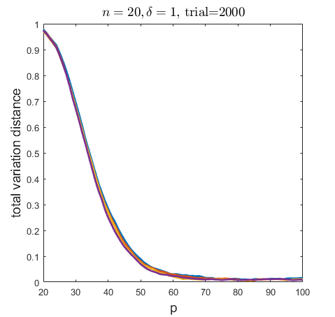
   Figure 3: The vertical axis is $d_{\operatorname{TV}}(\mathscr{L}\left({N_{V_{\delta}}^{(\bm{\Psi})}}\right),\operatorname{CP}(\lambda_{n,\delta}(1),\bm{\zeta}_{n,\delta}))$. The samples are independently generated according to $\mathcal{N}(\bm{0},\bm{\Sigma})$ with $\bm{\Sigma}$ being $(\tau,\kappa)$ sparse. The threshold $\rho$ is chosen according to (LABEL:eqn:rhopformula) with $e_{n,\delta}=1$. We fix $\kappa=p^{0.8}$ and vary $\tau$ in $p^{0.6},p^{0.4},p^{0.2},0$. Note $\tau=0$ means that $\bm{\Sigma}$ is the identity matrix. The four choices of $\tau$ correspond to the four curves in the plot. But the four curves highly overlapped and thus from this particular experiment we see that the accuracy of the non-asymptotic compound approximation is not sensitive to $\tau$.

   Figure 4 illustrates the the compound Poisson approximation for different values of $\kappa$, and the simulation indicates that the approximation accuracy is not sensitive to $\kappa$.

   

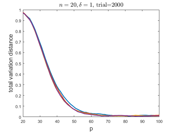
   Figure 4: The vertical axis is $d_{\operatorname{TV}}(\mathscr{L}\left({N_{V_{\delta}}^{(\bm{\Psi})}}\right),\operatorname{CP}(\lambda_{n,\delta}(1),\bm{\zeta}_{n,\delta}))$. The samples are independently generated according to $\mathcal{N}(\bm{0},\bm{\Sigma})$ with $\bm{\Sigma}$ being $(\tau,\kappa)$ sparse. The threshold $\rho$ is chosen according to (LABEL:eqn:rhopformula) with $e_{n,\delta}=1$. We fix $\tau=p^{0.6}$ and vary $\kappa$ in $p^{0.8},p^{0.5},p^{0.2},1$. Note $\kappa=1$ means that $\bm{\Sigma}$ is the identity matrix. The four choices of $\tau$ correspond to the four curves in the plot. But the four curves highly overlapped and thus from this particular experiment we see that the accuracy of the non-asymptotic compound approximation is not sensitive to $\kappa$.

   Furthermore, in our response to the Referee’s Comment # 2, we have provided numerical simulations for the case that sparsity assumption is violated. Please refer there for the details.

   Finally, as mentioned in our response to the Referee’s Comment #1, our theoretical results are invariant to the choice of $\bm{\mu}$ and $g$, as proved and discussed in detail in Lemma LABEL:lem:Uscoresdistribution and Remark LABEL:rem:Udisconsequence. As a result, we are in a position to respond to the reviewer’s comments in the affirmative, that is our results go through regardless of $g$ (or $\bm{\mu}$).

   Notwithstanding the interest of the affirming numerical results in Figures 1-4 in this response, we do not think that this theory paper is the appropriate venue for such empirical mathematical arguments.

4 Responses to Referee 3’s comments (filename: IT-21-0152-rev.pdf)

1. Comment The paper is very carefully written. It might even be a bit too pedantic in places, as the core message is not too surprising for people that are familiar with the general area, and this makes the paper difficult to read in many places (see below). Some of the comments, however, lack depth, in that the paper describes what it does but does not make connections with other areas of random graph theory where degree sequences are studied and, sometimes, shown to converge to a Poisson or mixed Poisson distribution.
   

   Response We are glad that the Referee found the paper to be very carefully written but we are sorry to hear that the Referee thinks “the core message is not too surprising for people that are familiar with the general area”. We apologize that we did not originally adopt an exposition that best conveyed our major contributions. To clarify our contributions, we have added a subsection in the introduction, which was quoted in our response to the AE. For the Referee’s benefit we replicate this quote below:

   We summarize the principal contributions of the paper. As above $p$ denotes the number of variables and $n$ denotes the number of samples.

   1. The paper presents a unified and complete asymptotic analysis of the star subgraph counts, the counts of vertices of a given degree and the counts of vertices above a given degree in the random graphs obtained by thresholding the sample correlation and sample partial correlation. This unification of different types of random counts represents an important improvement over previous work [hero2011large, hero2012hub] where only the counts of vertices above a given degree are studied.

   2. We approximate the full distributions of the random counts for finite $p$ and as $p\to\infty$. In addition, we characterize the first and second moments of these random counts. This is a significant generalization of previous results [hero2011large, hero2012hub] that only established approximations for the mean number of random counts and for the probabilities that these counts were positive.

   3. We obtains compound Poisson characterizations of the the distributions of the random counts. The compound Poisson limit and approximation are well approximated by the standard Poisson limit when $n$ is moderately large (Section LABEL:sec:limitingcompoundPoisson). This result corrects and refines the claim in [hero2012hub] that erroneously asserted a Poisson limit.

   4. The theory in this paper is developed under a novel sparsity condition on the population dispersion matrix. This sparsity condition, called $(\tau,\kappa)$ sparsity in Sec. LABEL:sec:taukappaspa, is significantly weaker than previously assumed conditions, which makes our theory more broadly applicable. Specifically, while the block sparsity condition in previous work [hero2012hub, fan2008sure, firouzi2016two] imposes that correlation can only occur locally in small blocks of variables, the $(\tau,\kappa)$ sparsity condition relaxes this condition to more general global correlation patterning.

   The implications of above technical contributions are far reaching. We elaborate on these implications below.

   Previous conditions on population partial correlation networks assume they are of lower dimension. In particular, conditions such as block sparsity do not allow for completely connected partial correlation graphs which involve all $p$ variables. Such restrictive assumptions are difficult to validate and rule out many realistic population (partial) correlation structures. Overcoming this hurdle has been an open problem for several years. The newly introduced $(\tau,\kappa)$ sparsity condition on the population covariance matrix settles this longstanding problem by successfully allowing for completely connected partial correlation graphs over the entire set of features. It therefore marks a significant theoretical breakthrough with important implications for correlation screening approaches in application domains.

   Historically, the literature on correlation estimation and graphical models has separated the treatments of covariance graph models and undirected graphical models (or inverse covariance graph models) [cox2014multivariate]. Unifying the two classes of statistical models has been an open problem for the better part of almost 3 decades. While this separate treatment may be appropriate in low dimensional settings when there are few variables, it is not immediately obvious which of the two frameworks is appropriate for a given data set in modern ultra-high dimensional regimes. To our knowledge, the framework in this paper is the first in the graphical model or correlation graph estimation literature to propose methodology which brings both approaches under one umbrella.

   The results in the paper also have significant relevance to applications. Recall that our Poisson and compound Poisson expressions effectively describe the number of false discoveries and hence allow us to obtain results for the familywise error rate (FWER) or k-FWER, that is the probability of obtaining k or more false discoveries. Note that we can also obtain the marginal distributions of correlation estimation which in turn allow us to obtain expressions for p-values for testing correlation estimates. These marginal p-values allow us to establish FDR control too using either the Benjamini-Hochberg [benjamini1995controlling] or Benjamini-Yakutelli procedures [benjamini2001control]. In summary, the correlations screening framework is sufficiently rich that it allows us to undertake statistical error control in terms of FWER, k-FWER and FDR. This is one of the main strengths of our results: a rigorous inferential framework in the ultra-high dimensional setting.

   We are not sure why the Referee thinks our results are not too surprising. The conclusions obtained in our paper were indeed quite surprising to us for a number of reasons. For example, the (incorrect) Poisson approximation from previous work [hero2012hub] had been accepted as the correct limiting distribution - not just by ourselves, but by many others who had used the work. Had the Poisson result been obviously incorrect and the compound Poisson been the obvious alternative, it would have made sense for the community to challenge the incorrect result and immediately correct it - but since this did not happen, we and others did not see the appropriateness of the compound Poisson right away. It only came about after careful analysis. In summary, the results in the paper were not so obvious to us.

   We next address your comment: “Some of the comments, however, lack depth, in that the paper describes what it does but does not make connections with other areas of random graph theory where degree sequences are studied and, sometimes, shown to converge to a Poisson or mixed Poisson distribution.” We are somewhat confused by this comment since we feel that we had specifically addressed the connections to random geometric graphs in a dedicated paragraph (quoted below) in Section LABEL:sec:rangeo. We feel that the connection and the comparisons between our models and the existing random geometric graphs are covered in the sense that, while for the cognoscenti, existing results might motivate our conclusion, our model and hypotheses (and thus our proofs) are quite different from those used in random graph theory. We have added the content highlighted in red to further clarify these connections.

   The random pseudo geometric graph in Definition LABEL:def:pge is similar to the random geometric graph introduced in [penrose2003random]. In particular, studied in the monograph [penrose2003random] is the number of induced subgraphs isomorphic to a given graph, typical vertex degrees, and other graphical quantities of random geometric graphs. As a specific example, the rate $a_{n}2^{n/2}p^{1+\frac{1}{\delta}}(1-\rho)^{\frac{n-2}{2}}\to e(n,\delta)$ as $p\to\infty$ in Theorem LABEL:cor:Poissonlimit is equivalent to $2a_{n}p^{1+\frac{1}{\delta}}r_{\rho}^{{n-2}}\to e(n,\delta)$, which is consistent with existing Poisson approximation for random geometric graph [penrose2003random, Theorem 3.4]. The differences between our random pseudo geometric graph in Definition LABEL:def:pge and the random geometric graphs defined in [penrose2003random] are: 1) our graph has vertices $\bm{u}_{i}$ lying on the unit sphere instead of on the entire Euclidean space; 2) our graph is induced by distance $\textbf{dist}(\cdot,\cdot)$ instead of the Euclidean distance. Another key difference is that vertices $\bm{u}_{i}$ are not necessarily independent in Definition LABEL:def:pge. Indeed in our model, the correlations between vertices $\bm{u}_{i}$ are encoded by a sparse matrix $\bm{\Sigma}$ (cf. Lemma LABEL:lem:Uscoresdistribution LABEL:item:Uscoresdistributiona), whereas in [penrose2003random] the vertices associated with the random geometric graph are assumed to be i.i.d. In [penrose2003random] it was stated (Example after [penrose2003random, Corollary 3.6]) without proof that the number of vertices with degree at least $3$ was approximately compound Poisson. A similar compound Poisson limit is established in Theorem LABEL:cor:Poissonlimit. There is some recent work on testing whether a given graph is a realization of Erdő s–Rényi random graphs or a realization of random geometric graphs with vertices i.i.d. uniformly distributed on the sphere; see [bubeck2016testing] and the reference therein.

   Two related comments are the Referee’s Other Comments # 8 and # 10, addressed in detail below, where some papers on random graphs are suggested by the Referee. For the Comment # 8, we agree that it is related and therefore we added the last sentence of the above paragraph, colored in red. But we do not see this missing reference as a paper very closely related paper to support the Referee’s claim in the comment. We address the relationship to Other Comments # 10 in the next paragraph.

   Finally, we point out that our results differ substantially from Chapter 6 of the van der Hofstadt book (in your Comment # 10) that shows convergence of a different limit (Poisson or mixed Poisson) of a different class of random graphs. We provide more details below in our response to our response to the Referee’s Comment # 10.

2. Comment The mathematics are carefully laid out over many pages of calculations that develop a (com- pound) Poisson approximation for, essentially, the degree sequence of a sparse correlation graph. The paper, in Section III in particular, tries to give an intuition for the proof arguments, but I think fails very short of that. What is the difference with basic Poisson approximation theory (e.g., [34])?
   

   Response We appreciate your comment that we had carefully laid our our mathematical arguments, and we did this so as to provide the most complete and reproducible presentation to the reader. In regards to your comments about subsection LABEL:sec:closenessnumedge, which attempted to provide intuition for the proof arguments, we have moved it to the Appendix (Sec. LABEL:sec:derivationprop:edgecor) in the revision. In response to your comment on the difference of our model with respect to the basic Poisson approximation theory of [34], as pointed out in our response to your Comment # 1, in Section III-B of the submitted version we have included a paragraph (see our response to your Comment # 1) dedicated to making comparisons between our random pseudo geometric graph models and the random geometric graphs studied in [penrose2003random] ([34] in the original submission). Please see our response to your Comment 1 for the quote of that paragraph. We point out that this informal derivation is in fact more closely related to the arguments used in [barbour2001topics] ([33] in the submitted version) than it is to [penrose2003random] ([34] in the submitted version) and this is why it required introducing additional notation.

3. Comment My main concern is the novelty. The improvement over [19] (described bottom page 5 - top page 6) is rather incremental. I do not doubt that the improvement is technical, but [19] was already published in IEEE IT. Is the topic so important that it warrants this? In addition the first paper in the line, [18], was published in JASA, a top statistics journal. If the contribution with respect to these papers is purely technical, then perhaps a more mathematically-oriented venue (a journal in probability theory) would be more appropriate.
   

   Response Admittedly we did not do a good job at clearly bringing out our contribution and novelty with respect to prior work. In the revision we have made changes to emphasize the novelty, key contributions, and comparisons with the prior work [18,19]. Please see our response to your Comment 1 for details. We do not believe that our contributions are incremental. Rather, we believe our manuscript represents significant progress on this important problem since it unifies and extends previous results, corrects previous results, has stronger conclusions than previous results, and weakens the assumptions necessary to obtain the previous results. The implications of above technical contributions in our response to your Comment # 1 are far reaching.

Comment So I am rather lukewarm about the paper, even though it’s easy to recognize that a lot of careful work has gone into it.

Response We trust that our careful summary of our significant contributions will paint a positive picture of the novelty of the results in the paper. We take responsibility for not bring these out in our original submission of the paper and apologize for this. We have responded to all the comments of the Referee carefully and also modify our original submissions accordingly, including but not limited to adding a new subsection to clarify the main contribution, moving some informal arguments to the appendix, adding some suggested references, improving some notations. We are hopeful that our responses and modifications will result in a warmer reaction by the Referee to our revised paper.

Other comments

1. Comment The bibliography is perhaps a bit incomplete as few works on sparse covariance matrix estimation are cited. There are also works that are closely and very closely related, such as the following, that are missing:
   Arias-Castro, E., Bubeck, S., & Lugosi, G. (2012). Detection of correlations. Annals of Statistics, 40(1).
   Fan, J., Shao, Q. M., Zhou, W. X. (2018). Are discoveries spurious? Distributions of maximum spurious correlations and their applications. Annals of Statistics, 46(3).
   The work here is instead presented as building on work by some of the authors [18, 19].
   

   Response Thanks for suggesting the two related references. After reading both papers, we see that there are connections at a superficial level, i.e., they also consider sample covariance matrices in high dimensions. These papers provide additional evidence that the general problem of correlation mining is important and of broad interest, so in the revision we have included these references in the last sentence of the first paragraph on page 2:

   The reader is referred to [anandkumar2009detection, castro2014detection, tan2014learning, heydari2017quickest, tarzanagh2018estimation, arias2012detection, fan2018discoveries] and the references therein for additional work related to high dimensional sample correlation matrices.

   However, we do not see the close relation that the Referee claimed. We point out that the fact that these papers did not cite our previous work [hero2011large] or [hero2012hub] ([18,19] in the submitted version of our paper), indicating that these authors did not themselves think their work was closely related to [hero2011large, hero2012hub] ([18,19] in the submitted version of our paper). Moreover, their models assumptions and results are very different.

2. Comment I do not understand the sentence “We define the set …” on page 3. The notation up to that point is strange. Why not $\bm{R}$ in place of $\bm{\Psi}^{(\bm{R})}$? That whole paragraph could be simpler. I would define $\mathcal{G}_{\rho}(\bm{\Psi})$ for any n-by-n matrix $\bm{\Psi}$, for example.
   

   Response We agree with you that “$\bm{R}$ in place of $\bm{\Psi}^{(\bm{R})}$” is simpler. We have implemented these changes in the revision. Thanks for the suggestion.

3. Comment $\mathcal{VE}$ for vector-elliptical is rather confusing in the presence of $(\mathcal{V},\mathcal{E})$ for a graph.
   

   Response Thanks for pointing this out. We have changed $(\mathcal{V},\mathcal{E})$ to be $(\mathrm{V},\mathrm{E})$

4. Comment Again, the notation could be improved. For example, in $\Ge(\{v_{i}\},r;n-2)$, unless I am missing something, the ”n-2” part is already given implicitly in that it is the dimension of the space where the points $v_{i}$ reside.
   

   Response We agree with you and have implemented the changes. Thanks for the suggestion.

5. Comment In (7), a different summation variable needs to be used (other than $\ell$).
   

   Response We have updated the variable. Thanks for pointing this out.

6. Comment Again, $\delta$ in this part of the paper is less than optimal, having been recently used to denote something very different.
   

   Response We are confused by your comment. Do you mean the $\delta$ in (7)? If yes, the $\delta$ in (7) is the hub level $\delta$ and there is no conflict in notation that we can see.

7. Comment Section II.D is not particularly enlightening.
   

   Response Section LABEL:sec:upperboundjointdensity presents some simple observations and examples for the new concept of local normalized determinant, which is used in Theorem LABEL:cor:Poissonlimit. To clarify the role of this section in the paper, we have added the following sentence in the first paragraph of Section LABEL:sec:upperboundjointdensity

   The normalized determinant measures the closeness between the identity matrix and the dispersion parameter $\bm{\Sigma}$. This plays an important role in Theorem LABEL:cor:Poissonlimit.

8. Comment In regards to Section III.B, the authors must know that (random) geometric graphs have been considered in settings other than the Euclidean setting. In particular, there is a line of work on testing a random graph (Erdő s–Rényi) vs a random geometric graph on the (high- dimensional) sphere, which the authors might find interesting as it is somewhat related to the topic at hand. See the following paper and others that cited it:
   Bubeck, S., Ding, J., Eldan, R., & Rácz, M. Z. (2016). Testing for high-dimensional geometry in random graphs. Random Structures Algorithms, 49(3).
   

   Response Thanks for bringing this interesting paper to our attention. The suggested paper is clearly related since they also study random geometric graph with vertices i.i.d. uniformly distributed on the sphere. The difference is that our model as a random pseudo geometric graph is defined in terms of a pseudo distance $\textbf{dist}(\bm{v}_{i},\bm{v}_{j}):=\min\left\{\|\bm{v}_{i}-\bm{v}_{j}\|_{2},\|\bm{v}_{i}+\bm{v}_{j}\|_{2}\right\}$ instead of the Euclidean distance, and our model allows possible correlation between vertices while theirs does not. We have added the following sentence in Section LABEL:sec:rangeo where we discuss the existing literature of random geometric graphs.

   There is some recent work on testing whether a given graph is a realization of a Erdő s–Rényi random graph or a realization of a random geometric graph with vertices i.i.d. uniformly distributed on the sphere; see [bubeck2016testing] and the reference therein.

   Note that one could potentially choose any of the random counts studied in our paper as a test statistic in their problem setting using our results. One may be able to characterize the distribution of the test statistic under the alternative hypothesis. Our paper can also potentially inspire people to study random geometric graphs with possible dependence among vertices of the random geometric graphs in their problem setting.

9. Comment Prop III.9 (b), do the constants in the bound also depend on $c$?
   

   Response Indeed this is an insightful comment. The constants in the upper bound of Proposition LABEL:thm:allclose do not depend on $c$. As discussed in Remark LABEL:rem:allclose, the condition that involves $c$ is a quantitative way of saying that $p$ is sufficiently large. So if $c$ is sufficiently small, which implies that $p$ is sufficiently large, then the inequality in the conclusion of Proposition LABEL:thm:allclose LABEL:item:allclosec is valid. However the constants in the upper bound do not functionally depend on $c$.

   To further clarify this point, we have written “positive and sufficiently small $c$” in the statement of Proposition LABEL:thm:allclose LABEL:item:allclosec, and also added the following sentence in Remark LABEL:rem:allclose:

   The inequalities (LABEL:eqn:allclosec) and (LABEL:eqn:allclosed) are valid as long as $c$ is less than finite constant, given respectively in (LABEL:eqn:cdef) and (LABEL:eqn:cuppbou2) in the supplementary material [hero2020unified] to this paper.

   We have also updated other related places in the paper to be “positive and sufficiently small $c$”.

10. Comment Section III is hard to read because of the large amount of notation introduced there… and the payoff is not at all clear. I did not get any clear intuition on proof arguments beyond how typical Poisson approximations work — which I am somewhat familiar with, at least at the level of [34]. It would have been more instructive to understand how the setting differs from the usual Poisson approximation setting, and perhaps draw some relations with what is known for generalized random graphs (see the book by van der Hofstad, Ch 6).
    

    Response We think this is related to your major Comment #2. We have discussed in great detail the differences between our informal arguments and the book [34] in our response to your major Comment 2. We also moved the informal derivation to the appendix. Please refer to our responses to your major Comment 2 for more details.

    Relative to the last sentence of your comment, Chapter 6 of the van der Hofstadt book covers a very different class of random graphs than the random pseudo-geometric graphs to which the theory in our paper applies. The class of random graphs in Ch. 6 of the reference are called generalized random graphs and, similarly to other inhomogeneous versions of the Erdos-Renyi graph, the edges are random and drawn indpendently with probabilities $p_{ij}$ of there existing an edge between vertices $i$ and $j$. Specifically, for the generalized random graph $p_{ij}=W_{i}W_{j}/(L_{n}+W_{i}W_{j})$ where $W_{i}\geq 0$ is a scalar attribute (called a weight in Ch. 6 of the reference) and $L_{n}=\sum_{i=1}W_{i}$. On the other hand the random pseudo-geometric graph studied in our paper has random edges that are dependent with marginal probability $p_{ij}$ equal to threshold exceedance probability of the magnitude correlation or partial corelation between vector-valued vertex attributes $X_{i}$ that follow a elliptically contoured multivariate distribution. In Sec 6.3 van der Hofstadt obtains a mixed Poisson limiting distribution for the vertex degree. The mixed Poisson and the compound Poisson are very different distributional limits for the vertex counts of two very different random graph models.

11. Comment Similarly, what is the utility of Section V? Isn’t the approximation of a compound Poisson distribution with a Poisson distribution well-understood? I would have liked to see some numerical experiments, perhaps using genetics data, on how accurate and useful the formulas developed in the paper are. After all, the paper is motivated by such applications. The discussion (Section VI) mentions some numerical experiments. (I am completely fine with a purely theoretical paper, but then, what is the purpose of Section V?)
    

    Response Yes, you are right that the paper is envisioned to be a purely theoretical paper. As stated at the beginning of Section LABEL:sec:limitingcompoundPoisson, the purpose of this section is provide useful approximations to the parameters (are defined in terms of random geometric graphs) for the compound Poisson in the context of the sample correlation graph. The main contribution in Section LABEL:sec:limitingcompoundPoisson lies in Lemma LABEL:lem:randgeogra and Lemma LABEL:lem:randgeograconduppbou, for which we apply concentration inequalities to random (pseudo) geometric graphs. To the best of our knowledge, these two lemmas are novel and we think they are quite interesting. That we obtain a Poisson approximation to the compound Poisson distribution is not our goal/purpose in Section LABEL:sec:limitingcompoundPoisson, but is rather a consequence or a byproduct of the estimation/approximation to the complicated quantity in the random (pseudo) geometric graphs established in Lemma LABEL:lem:randgeogra and Lemma LABEL:lem:randgeograconduppbou.

    However, if the Referee thinks Section LABEL:sec:limitingcompoundPoisson is well-understood in the literature, please provide a specific resource that has the same or similar results, and we would be happy to update the section accordingly.

5 Responses to Referee 4’s comments (filename: IEEE Trans Inf Theory report.pdf)

Comment I found the paper pretty interesting and felt that it definitely made novel contributions. The paper was quite comprehensive and thorough in its theoretical treatment of correlation and partial correlation screening. It definitely made interesting connections to random geometric graph theory. A lot of questions that I had while reading the paper were answered in the remarks of the paper or in the Appendices. However, I have a few concerns that I hope the authors can address, which I detail below.

Response Thank Referee for positive comments on the comprehensiveness and the thoroughness of our paper. We try to be as precise as possible while try to make the results accessible by providing many remarks. We have provided responses to the Referee’s specific concerns below.

1. Comment Theorem II.4, the authors require the correlation threshold $\rho$ to grow at a very specific function of $p$, i.e. $a_{n}2^{n/2}p^{1+\frac{1}{\delta}}(1-\rho)^{\frac{n-2}{2}}\to e(n,\delta)$ as $p\to\infty$. This seems to be an artifact of the proof, and it is a bit troubling (even though the authors pointed out later that the growth rate is not fast). Is this a sharp rate, i.e. can this condition not be relaxed at all? Does the distributional limit result automatically fail when this condition on the growth rate of $\rho$ does not hold? This deserves greater attention, and the authors may want to prove that this rate is sharp when $p\to\infty$. Otherwise, it raises a lot of questions and concerns.
   

   Response This rate is not an artifact of the proof, it is a sharp rate. From Section LABEL:sec:rangeo we know that our model is a Random Psuedo Geometric Graph with radius parameter $r_{\rho}=\sqrt{2(1-\rho)}$. Thus the rate is equivalent to $2a_{n}p^{1+\frac{1}{\delta}}r_{\rho}^{{n-2}}\to e(n,\delta)$, which is consistent with existing Poisson approximations for random geometric graphs [penrose2003random, Theorem 3.4]. We have added such discussions in Section LABEL:sec:rangeo:

   As a specific example, the rate $a_{n}2^{n/2}p^{1+\frac{1}{\delta}}(1-\rho)^{\frac{n-2}{2}}\to e(n,\delta)$ as $p\to\infty$ in Theorem LABEL:cor:Poissonlimit is equivalent to $2a_{n}p^{1+\frac{1}{\delta}}r_{\rho}^{{n-2}}\to e(n,\delta)$, which is consistent with existing Poisson approximation for random geometric graph [penrose2003random, Theorem 3.4].

   In Remark LABEL:rem:remarkofthm1 we also added:

   This particular rate on $\rho$ is consistent with the rate of the existing Poisson approximation results in random geometric graphs [penrose2003random] as will be discussed in Section LABEL:sec:rangeo.

   The rate is sharp in the sense that letting $\rho$ grow at a faster or slower rate the result will be a degenerate compound Poisson limit (a limit either having mean 0 or mean $\infty$). This was briefly discussed in Lemma LABEL:lem:compoundpoissonlimit in the submitted paper. For the benefit of the Referee, we provide some additional details on the sharpness of this rate that we choose not to include in the revision. Since we want to establish a result that holds for a certain type sparse dispersion parameter $\bm{\Sigma}$, we specialize to the special case that $\bm{\Sigma}$ is diagonal in the following derivation. By Lemma LABEL:lem:meanedge with $\kappa=1$ (note that diagonal matrix is row-$\kappa$ sparse with $\kappa=1$), we have

   $$\mathbb{E}N_{E_{\delta}}^{(\bm{R})}=\mathbb{E}Z=\binom{p}{1}\binom{p-1}{\delta}(2P_{n}(r_{\rho}))^{\delta},$$

   which behaves the same as $\frac{1}{\delta!}(2p^{1+\frac{1}{\delta}}P_{n}(r_{\rho}))^{\delta}$ when $p$ is large. By Lemma LABEL:pderivative LABEL:item:pderivativeb, we further have when $p$ is large

   $$\mathbb{E}N_{E_{\delta}}^{(\bm{R})}\approx\frac{1}{\delta!}\left(2p^{1+\frac{1}{\delta}}a_{n}(1-\rho)^{\frac{n-2}{2}}\right)^{\delta}.$$

   Thus in order to have a non-degenerate mean when $p\to\infty$, $2p^{1+\frac{1}{\delta}}a_{n}(1-\rho)^{\frac{n-2}{2}}$ needs to converges to some strictly positive and finite constant. Thus the rate we give in Theorem LABEL:cor:Poissonlimit is sharp. We hope this simple derivation addresses the concerns.

2. Comment As the authors point out, the compound Poisson characterization holds for the vertex counts in the empirical correlation graphs under the much weaker row-$\kappa$ sparsity (Lemmas II.5 and Lemma III.12). So clearly the $(\tau,\kappa)$ assumption is an important one to make for the other four random counts. Why is it that we need the $(\tau,\kappa)$ assumption for the counts besides the vertex counts of the empirical correlation graphs? This should be clarified, so that we know why we need to consider $(\tau,\kappa)$ sparsity instead of just the weaker row-$\kappa$ sparsity (which seems more realistic in the “large p” setting).
   

   Response We do not understand why you said “So clearly the $(\tau,\kappa)$ assumption is an important one to make for the other four random counts.” There are totally $6$ random counts studied in our paper, and three random counts associated with the empirical correlation graph were treated in Lemma LABEL:item:Poissonultrahigha under the weaker row-$\kappa$ sparsity. The other $3$ counts associated with the empirical partial correlation graph are the ones that uses the $(\tau,\kappa)$ assumption. So we are not sure why the Referee mentioned ”the other four random counts” in the comment. Currently we are not aware of any proof without $(\tau,\kappa)$ sparse assumption for the empirical partial correlation graph, although numerical experiments (see Figure 1 and Figure 2 in our response to Referee 2’s Comment # 2) suggest that the conclusion still holds beyond $(\tau,\kappa)$ sparse assumption.

3. Comment In modern high-dimensional problems, it is common not only for $p$ to be large but also $n$. The authors only consider fixed n but allow $p$ to diverge to $\infty$. Can the results in this paper be extended to the case where both $n$ and $p$ are growing? Do they still hold if $n$ grows (much) slower than $p$? If this is not the case, then the authors could explain what the technical challenges are with characterizing the limiting distributions when we allow $n$ to also diverge with $p$.
   

   Response This is an interesting question. The answer is yes, we think that the results still hold when $n$ grows (much) slower than $p$. Take Proposition LABEL:prop:edgecor for example. As mentioned in Remark LABEL:rem:edgecor, “Respective expressions for $C^{\prime}_{\delta,\gamma}$ and $C_{n,\delta,\rho}$ in Proposition LABEL:prop:edgecor are presented in equations (LABEL:eqn:C'delgamdef) and (LABEL:eqn:Cndelgamdef) in the Supplementary Material ([hero2020unified])”. One could then just plug those formulae into the upper bound in Proposition LABEL:prop:edgecor, and one should be able to prove that the upper bound can go to $0$ with suitable condition on $\mu_{n,2\delta+2}\left(\bm{\Sigma}\right)$ (note that a sufficient condition to control $\mu_{n,2\delta+2}\left(\bm{\Sigma}\right)$ is given in Lemma LABEL:lem:sufass). So in principle $n$ can also approach infinity.

   However, since the current manuscript is already quite long, we believe that the interesting case that $n$ and $p$ both approach infinity is best deferred to a future paper.

4. Comment I know that this is a theoretical paper, but I am curious if the authors could discuss further some of the practical implications of their findings. The authors briefly mention that their method can be used to approximate the family-wise error rate (FWER), but this is presented rather lightly in the manuscript. The authors may want to highlight this more, so it is not just seen as an interesting theoretical result, but also has some important implications for practitioners who employ correlation or partial correlation screening. Is there anything else that the limiting compound Poisson distribution of these vertex counts (or their Poisson approximations) tell us? For example, can we use these distributions for inference and hypothesis testing? Moreover, since FWER is known to be very conservative, there seems to be more interest in modern settings for controlling the false discovery rate (FDR) instead. Can the theory in this paper help to inform efforts to control the false detection rate of vertices of degree exceeding $\delta$?
   

   Response The reviewer makes very insightful remarks, and these insights are well placed: the results in our paper are not just of a technical nature, they also have tremendous practical implications, once again underscoring the substantive and non-incremental nature of the contributions in the paper. Our results can definitely be used to quantify the FWER, and as the reviewer points out, this multiple hypothesis testing error metric is sometimes viewed as overly conservative. This poses no problem for our results as we have expressions for k-FWER, the probability of obtaining k or more false discoveries. This multiple hypothesis testing error metric is naturally less conservative than simple FWER and addresses the reviewer’s concerns. In particular, our Poisson and compound Poisson expressions effectively describe the number of false discoveries and hence allow us to obtain results for k-FWER. Note that we can also obtain the marginal distributions of correlation estimation which in turn allow us to obtain expressions for p-values for correlation parameters. These marginal p-values allow us to establish FDR control too using either the Benjamini-Hochberg [benjamini1995controlling] or Benjamini-Yakutelli procedures [benjamini2001control]. In summary, the correlations screening framework is sufficiently rich that it allows us to undertake statistical error control in terms of FWER, k-FWER and FDR. This is one of the main strengths of our results: a rigorous inferential framework in the ultra-high dimensional setting. We have followed the reviewer’s advice and have highlighted the practical implications of the results in the paper as follows:

   The results in the paper also have significant relevance to applications. Recall that our Poisson and compound Poisson expressions effectively describe the number of false discoveries and hence allow us to obtain results for the familywise error rate (FWER) or k-FWER, that is the probability of obtaining k or more false discoveries. Note that we can also obtain the marginal distributions of correlation estimation which in turn allow us to obtain expressions for p-values for testing correlation estimates. These marginal p-values allow us to establish FDR control too using either the Benjamini-Hochberg [benjamini1995controlling] or Benjamini-Yakutelli procedures [benjamini2001control]. In summary, the correlations screening framework is sufficiently rich that it allows us to undertake statistical error control in terms of FWER, k-FWER and FDR. This is one of the main strengths of our results: a rigorous inferential framework in the ultra-high dimensional setting.