A novel analytic atmospheric $T(\tau)$ relation for stellar models

Abstract

Stellar models often use relations between the temperature $T$ and optical depth $\tau$ to evaluate the structure of their optically-thin outer layers. We fit a novel analytic function to the Hopf function $q(\tau)$ of a radiation-coupled hydrodynamics simulation of near-surface convection with solar parameters by Trampedach et al. (2014). The fit is accurate to within $0.82$ per cent for the solar simulation and to within $13$ per cent for all the simulations that are not on either the low-temperature or low-gravity edges of the grid of simulations.

Standard one-dimensional stellar models require a boundary condition that summarises the transition from their opaque depths to their observable outer layers. These are usually provided by either (a) tables of surface pressure and temperature computed using separate codes that model the complicated physics of stellar atmospheres or (b) $T(\tau)$ relations that specify the stratification of the temperature $T$ as a function of the optical depth $\tau$. These $T(\tau)$ relations follow the general form

$$\left(\frac{T(\tau)}{T_{\mathrm{eff}}}\right)^{4}=\frac{3}{4}\left(\tau+q(\tau)\right)$$ (1)

where $T_{\mathrm{eff}}$ is the effective temperature and $q(\tau)$ is a Hopf function. We denote the optical depth at which $T=T_{\mathrm{eff}}$ by $\tau_{\mathrm{eff}}$. Hopf functions can be derived theoretically given some assumptions (e.g. the Eddington model $q(\tau)=2/3$) or fit to data or detailed atmosphere models. Two common $T(\tau)$ relations, besides the Eddington relation, are those of Krishna Swamy (1966) and analytic fits to Model C by Vernazza et al. (1981), known as VAL-C (see e.g. Paxton et al., 2013; Sonoi et al., 2019).

In the study of solar-like oscillations, the atmosphere’s structure can affect the mode frequencies appreciably and must therefore be included in the equilibrium stellar models. This can be done by integrating the equations of the atmosphere’s structure and appending the integrated structure to the interior model. Alternatively, one can modify the stellar structure equations and extend the model to smaller optical depths. Specifically, one multiplies the radiative temperature gradient $\nabla_{\mathrm{rad}}=(\partial\ln T/\partial\ln P)_{\mathrm{rad}}$ by $1+\mathrm{d}q/\mathrm{d}\tau$ (see e.g. Mosumgaard et al., 2018). The first method requires the Hopf function; the second requires its gradient.

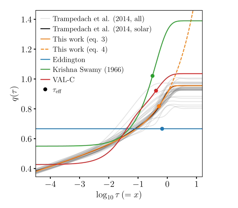
Trampedach et al. (2014) presented Hopf functions for a set of three-dimensional radiation-coupled hydrodynamics (3D RHD) simulations of near-surface convection, as well as routines that allow stellar modellers to interpolate the Hopf functions as a function of the surface gravity $\log g$ and effective temperature $T_{\mathrm{eff}}$. The simulated Hopf functions are most similar to that of VAL-C but do not tend to a constant temperature at small optical depths. While we encourage modellers to use the routines to interpolate in the full suite of Hopf functions, we present here an analytic function that allows relatively simple implementation of the solar Hopf function, which is itself somewhat representative of all the Hopf functions in the grid of models.

The gradient of the Hopf function for the simulation with solar parameters ($T_{\mathrm{eff}}=5775\,\mathrm{K}$, $\log g=4.438$) can be approximated by the function

$$\frac{\mathrm{d}q}{\mathrm{d}x}=\frac{c_{1}+e^{\frac{x-a}{v}}}{1+e^{\frac{x-b}{w}}}\mathrm{,}$$ (2)

where $x=\log_{10}\tau$. This motivates fitting the Hopf function using the integral of eq. 2 (Wolfram|Alpha, 2021),

$$q(x)=c_{0}+c_{1}\left(x-w\ln\left(e^{\frac{b}{w}}+e^{\frac{x}{w}}\right)\right)+v\,e^{\frac{x-a}{v}}\,{}_{2}F_{1}\left(1,\frac{w}{v};1+\frac{w}{v};-e^{\frac{x-b}{w}}\right)\mathrm{,}$$ (3)

where ${}_{2}F_{1}$ is the hypergeometric function. We found best-fitting parameters $c_{0}=0.6887302$, $c_{1}=0.0668698$, $a=0.9262126$, $b=0.1148743$, $v=0.7657857$ and $w=0.0514999$, with which the fit reproduces the data to within $0.82$ per cent over the full range $-4.5<x<2.0$. The fit is also fairly representative of all the simulations away from the low-temperature and low-gravity edges of the grid. If we exclude simulations with $T_{\mathrm{eff}}<4400\,\mathrm{K}$ or $\log g<T_{\mathrm{eff}}/1000\,\mathrm{K}-2.2$, the fit reproduces all the remaining Hopf functions within $13$ per cent.

The hypergeometric function in eq. 3 is not always practical but the term that contains it does not contribute to the function for $x\lesssim 0$. Ignoring this term is equivalent to ignoring the denominator in eq. 2, in which case the integral is

$$q(x)=c_{0}+c_{1}(x-b)+v\,e^{\frac{x-a}{v}}\mathrm{.}$$ (4)

This is also accurate to within $0.82$ per cent up to $x=0.0741$ for the solar model and to the same accuracy up to $\tau_{\mathrm{eff}}=0.5147929$. Thus, if integrating an atmosphere using $q(x)$, where one usually terminates at or below $\tau_{\mathrm{eff}}$, the approximate formula in eq. 4 can be used. If including the atmosphere’s structure by modifying the structure equations, then the full equation of the gradient (eq. 2) must be used because we require $\mathrm{d}q/\mathrm{d}\tau\to 0$ for $\tau\gg 1$.

Fig. 1 shows the Hopf functions we have discussed: the data from Trampedach et al. (2014), our fits of eqs 3 and 4 to their solar simulation, and the three widely-used $T(\tau)$ relations. Fig. 1 and most of the preceding analysis can be generated by a publicly available Python script (Ball, 2021).

Figure 1: All the Hopf functions $q(x)$ discussed, with the corresponding values of $\tau_{\mathrm{eff}}$ indicated by filled circles. The full set of simulations by Trampedach et al. (2014) is shown in light grey and their solar simulation in black. The solid orange line is our fit of eq. 3 to the data for the solar simulation and the dashed orange line the approximate function in eq. 4 using the same parameters. The blue, green and red lines are the popular Hopf functions for the standard Eddington atmosphere, the relation by Krishna Swamy (1966) and a fit to VAL-C (Vernazza et al., 1981; Paxton et al., 2013; Sonoi et al., 2019).

References

- Ball (2021) Ball, W. 2021, warrickball/atm_rnaas2021: Publication version, v1.0, Zenodo, doi: 10.5281/zenodo.4423991
- Harris et al. (2020) Harris, C. R., Jarrod Millman, K., van der Walt, S. J., et al. 2020, Nature, 585, 357, doi: 10.1038/s41586-020-2649-2
- Hunter (2007) Hunter, J. D. 2007, Computing In Science & Engineering, 9, 90, doi: 10.1109/MCSE.2007.55
- Krishna Swamy (1966) Krishna Swamy, K. S. 1966, ApJ, 145, 174, doi: 10.1086/148752
- Mosumgaard et al. (2018) Mosumgaard, J. R., Ball, W. H., Silva Aguirre, V., Weiss, A., & Christensen-Dalsgaard, J. 2018, MNRAS, 478, 5650, doi: 10.1093/mnras/sty1442
- Paxton et al. (2013) Paxton, B., Cantiello, M., Arras, P., et al. 2013, ApJS, 208, 4, doi: 10.1088/0067-0049/208/1/4
- Sonoi et al. (2019) Sonoi, T., Ludwig, H. G., Dupret, M. A., et al. 2019, A&A, 621, A84, doi: 10.1051/0004-6361/201833495
- Trampedach et al. (2014) Trampedach, R., Stein, R. F., Christensen-Dalsgaard, J., Nordlund, Å., & Asplund, M. 2014, MNRAS, 442, 805, doi: 10.1093/mnras/stu889
- Vernazza et al. (1981) Vernazza, J. E., Avrett, E. H., & Loeser, R. 1981, ApJS, 45, 635, doi: 10.1086/190731
- Virtanen et al. (2020) Virtanen, P., Gommers, R., Oliphant, T. E., et al. 2020, Nature Methods, 17, 261, doi: 10.1038/s41592-019-0686-2
- Wolfram|Alpha (2021) Wolfram|Alpha. 2021, Wolfram Alpha LLC. https://www.wolframalpha.com/input/?i=integrate+%28c1%2Bexp%28%28x-a%29%2Fv%29%29%2F%281%2Bexp%28%28x-b%29%2Fw%29%29