mirkwood: Fast and Accurate SED Modeling Using Machine Learning

Abstract

Traditional spectral energy distribution (SED) fitting codes used to derive galaxy physical properties are often uncertain at the factor of a few level owing to uncertainties in galaxy star formation histories and dust attenuation curves. Beyond this, Bayesian fitting (which is typically used in SED fitting software) is an intrinsically compute-intensive task, often requiring access to expensive hardware for long periods of time. To overcome these shortcomings, we have developed mirkwood: a user-friendly tool comprising of an ensemble of supervised machine learning-based models capable of non-linearly mapping galaxy fluxes to their properties. By stacking multiple models, we marginalize against any individual model’s poor performance in a given region of the parameter space. We demonstrate mirkwood’s significantly improved performance over traditional techniques by training it on a combined data set of mock photometry of z=0 galaxies from the Simba, EAGLE and IllustrisTNG cosmological simulations, and comparing the derived results with those obtained from traditional SED fitting techniques. mirkwood is also able to account for uncertainties arising both from intrinsic noise in observations, and from finite training data and incorrect modeling assumptions. To increase the added value to the observational community, we use Shapley value explanations (SHAP) to fairly evaluate the relative importance of different bands to understand why particular predictions were reached. We envisage mirkwood to be an evolving, open-source framework that will provide highly accurate physical properties from observations of galaxies as compared to traditional SED fitting.

1 Introduction

1.1 Traditional SED Fitting

Spectral energy distributions (SEDs) of galaxies are crucial in informing our understanding of the most fundamental physical properties, such as their redshifts, stellar population masses, ages, and dust content. The task of extracting these properties by fitting models of the stellar photometry and dust attenuation to observations of galaxies is commonly known as SED fitting, and is one of the most common ways of deriving physical properties of galaxies. In SED fitting, stellar populations are evolved with over an assumed star formation history (SFH), with an assumed stellar initial mass function (IMF) and through an assumed dust attenuation curve, to produce a composite spectrum. This resulting spectrum is then compared to the galaxy photometric observation under consideration, and the input assumptions are varied until there is a reasonable match between the two. The best fit model is then used to infer the physical properties of the concerned galaxy (see recent reviews by Walcher et al. 2011; Conroy 2013).

This technique has been transformational in turning observed data into inferred galaxy physical properties. For instance, we now understand the evolution of the galaxy stellar mass function through z $\sim 7$ (Tomczak et al., 2014; Grazian et al., 2015; Leja et al., 2019d), the diversity in shapes of galaxy SFHs (Papovich et al., 2011; Leja et al., 2019b), the nature of the star formation rate–stellar mass (SFR-M^⋆) relation through z = 2 (Mobasher et al., 2008; Iyer et al., 2018), the process of inside-out quenching (Jung et al., 2017), and the general shapes of galaxy dust attenuation curves at high-z (Salmon et al., 2016), all thanks to a combination of high quality data with SED fitting techniques. These developments have spurred – and in turn have been accelerated by – the development of modern SED fitting codes such as CIGALE (Boquien et al., 2019), Prospector (Leja et al., 2017), FAST (Kriek et al., 2009), BAGPIPES (Carnall et al., 2018), and MAGPHYS (Da Cunha et al., 2008). These codes rely on Bayesian optimization and Markov Chain Monte Carlo (MCMC) sampling methods to explore the large input base of computer simulated SED templates for close matches with an observed SED, and consequently output its physical properties.

At the same time, this traditional method of fitting SEDs has been known to introduce potential uncertainties and biases in the derived physical properties of galaxies. At the core of the issue are assumptions regarding the model stellar isochrones, spectral libraries, the IMF, the SFH, and the dust attenuation law. Each of these choices can dramatically impact the derived physical properties. For example, Acquaviva et al. (2015) evaluated the effects that different modelling assumptions have on the recovered SED parameters, and found that the incorrect parameterizations of the star formation history can significantly impact the derived physical properties. This finding has been confirmed by the works of Wuyts et al. (2009); Michałowski et al. (2014); Sobral et al. (2014) and Simha et al. (2014), who have all found significant impact of SFH on the derived galaxy stellar mass in various observational datasets. Pacifici et al. (2015) found that the simple assumption of exponentially declining SFH, simple dust law, and no emission-line contribution fails to recover the true stellar mass - star formation rate relationship for star-forming galaxies. Similarly, Iyer & Gawiser (2017) and Lower et al. (2020) found that fitting the SFH using simple functional forms leads to a bias of up to 70% in the recovered total stellar mass. In addition, Carnall et al. (2019) demonstrated that such simple functional forms for SFH also impose strong priors on other physical parameters, which in turn bias our inference for fundamental cosmic relations, such as the stellar mass function (SMF) and the cosmic star formation rate density (CSFRD, Ciesla et al. (2017); Leja et al. (2019a)), critical for answering crucial questions in the study of galaxy formation and evolution. Even with more complex SFH functions which have been able to better reproduce the CSFRD (Gladders et al., 2013), individual stellar age estimates have been biased (Carnall et al., 2019; Leja et al., 2019d). In a similar vein to SFH modeling, in their recent review Salim & Narayanan (2020) found that incorrect assumptions of the dust attenuation law, even within the commonly accepted family of locally-calibrated curves, can drive major uncertainties in the derived galaxy star formation rates.

To overcome some of these limitations of traditional SED fitting, two broad approaches have been introduced. The first has been to modify the SFH prior employed during SED fitting. This has been accomplished by either creating new functional, parametric forms for the SFH that result in lower biases in derived posteriors in physical parameters, for instance by being less subject to the ‘outshining bias’ (Behroozi et al., 2013; Simha et al., 2014), or by developing parameter-free (non-parametric) descriptions of the SFH (Tojeiro et al., 2007; Iyer & Gawiser, 2017; Iyer et al., 2019; Leja et al., 2019a). The latter are those that allow for a number of flexible bins of star formation to vary in the SED modeling procedure in order to model the more complex star formation histories that likely represent real galaxies (Iyer et al., 2018; Leja et al., 2019c). In Lower et al. (2020), the authors used a subset of the hydrodynamical simulations used in this work to study the biases introduced by various commonly used parametric forms of SFH on the derived stellar masses, and found that some of the most commonly used formulations – ‘constant’, ‘delayed-$\tau$’ and ‘delayed-$\tau$ + burst’ – dramatically under-predict the true stellar mass. They then compared the performance against that obtained by using a non-parametric SFH model (Leja et al., 2017), and found significantly better results. Even so, there were a large number of catastrophic outliers, with errors of up to 40% (see Figure 3 in their work). This is because SED fitting is inherently a complex task involving several moving parts, and SFH is only one of several model assumptions that go in it. As already mentioned, for example, the assumed dust attenuation law is another factor that can significantly impact the derived galaxy properties (see Figure 2 in Salim & Narayanan 2020).

The upshot is that the uncertainties in the galaxy star formation history and star-dust geometry (as manifested in their dust attenuation curves) translate to significant uncertainties in the derived properties from traditional SED fitting techniques (Lower et al., 2020; Leja et al., 2017, 2019a; Salim & Narayanan, 2020). An alternative to SED fitting is to instead derive a mapping between the photometry of a galaxy and the underlying physical properties. In this regard, machine learning techniques can serve as a potential alternative to traditional SED fitting. In this paper, we demonstrate that machine learning is not only a suitable alternative, but potentially more accurate one.

1.2 Machine Learning and SED Fitting

To explore the complex and degenerate parameter space more efficiently, machine learning (ML) has emerged as an alternative tool for deriving the physical parameters of galaxies. Unlike traditional SED fitting procedures, including those utilizing novel non-parametric SFH priors, ML algorithms are able to directly learn the relationships between the input observations (either photometric of spectroscopic) and the galaxy properties of interest without the need for human-specified priors. With ML, the priors themselves become learnable. This is possible because ML algorithms learn from the entire population ensemble, learning not just the mapping between individual galaxy observations and physical properties, but also the distribution of properties.

Lovell et al. (2019)) trained convolutional neural networks (CNNs, Krizhevsky et al. (2012)) to learn the relationship between synthetic galaxy spectra and high resolution SFHs from the Eagle (Schaye et al., 2015) and Illustris (Vogelsberger et al., 2014) simulations. Stensbo-Smidt et al. (2017) estimated specific star formation rates (sSFRs) and redshifts using broad-band photometry from SDSS (Sloan Digital Sky Survey, Eisenstein et al. (2011)). Surana et al. (2020) used CNNs with multiband flux measurements from the GAMA (Galaxy and Mass Assembly, Driver et al. (2009)) survey to predict galaxy stellar mass, star formation rate, and dust luminosity. Simet et al. (2019) used neural networks trained on semi-analytic catalogs tuned to the CANDELS (Cosmic Assembly Near-infrared Deep Extragalactic Legacy Survey, Grogin et al. (2011)) survey to predict stellar mass, metallicity, and average star formation rate. Owing to their superior ability in capturing non-linearity in data, ML-based models have seen applications in almost every field of astronomical study, including identification of supernovae (D’Isanto et al., 2016), classification of galaxy images (Cheng et al., 2020a, b; Hausen & Robertson, 2020; Ćiprijanović et al., 2020; Barchi et al., 2020), and categorization of signals observed in a radio SETI experiment (Harp et al., 2019). With the exponential growth of astronomical datasets, ML based models are slowly becoming an integral part of all major data processing pipelines (Siemiginowska et al., 2019). Baron (2019) provides a comprehensive and current overview of the application of machine learning methodologies to astronomical problems.

Table 1: Summary statistics of the five galaxy properties in this paper, for all three hydrodynamical simulations.

		Simba	Eagle	IllustrisTNG
	Min	7.64	7.64	7.70
	Max	12.15	12.01	12.19
$\log_{10}(\frac{\rm{M}^{\star}}{\rm{M}_{\odot}})$	Mean	8.91	8.71	8.82
	Median	8.78	8.50	8.65
	Std.Dev.	0.86	0.83	0.85
	Min	0.0	2.81	4.72
	Max	8.63	10.5	10.26
$\log_{10}(1+\frac{\rm{M}_{\rm{Dust}}}{\rm{M}_{\odot}})$	Mean	5.39	6.25	6.82
	Median	5.33	6.06	6.72
	Std.Dev.	1.47	0.86	0.75
	Min	-1.61	-1.05	-1.27
	Max	0.08	0.30	0.17
$\log_{10}(\frac{\rm{Z}^{\star}}{\rm{Z}_{\odot}})$	Mean	-0.86	-0.25	-0.49
	Median	-0.87	-0.24	-0.50
	Std.Dev.	0.35	0.18	0.28
	Min	0.0	0.0	0.0
	Max	1.35	1.14	1.57
$\log_{10}(1+\rm{SFR}_{100})$	Mean	0.10	0.05	0.09
	Median	0.02	0.01	0.03
	Std.Dev.	0.18	0.11	0.15
#Samples		1,797	4,697	10,073

1.3 This Paper

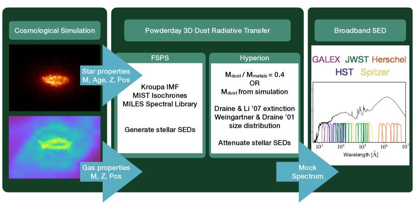
Figure 1: Data pipeline for each simulated galaxy. Once galaxies are selected from each simulation, we perform 3D dust radiative transfer with powderday, which utilizes fsps to generate the stellar SEDs and hyperion to propagate the stellar SEDs through a dusty medium dependent. We then sample mock photometry in $33$ filters from the powderday SED.

In this paper we introduce mirkwood, a fully ML-based tool for deriving galaxy physical parameters from multi-band photometry, while robustly accounting for various sources of uncertainty. We compare mirkwood’s performance with that of the current state-of-the-art Bayesian SED fitting tool Prospector, by using data from galaxy formation simulations for which we have ground-truth values. To do this, we first create mock SEDs from three different cosmological hydrodynamical simulations (via the procedure discussed in detail in Section 2 and illustrated in Figure 1) – Simba, Eagle, and IllustrisTNG. We then fit GALEX, HST, Spitzer, Herschel, and JWST photometry of these mock SEDs to extract stellar masses, dust masses, stellar metallicities, and instantaneous SFRs (defined as the mean SFR in the past 100 Myrs from the time of observation) using the publicly available SED fitting software Prospector (Leja et al., 2017) with the state-of-the-art non-parametric SFH model from Leja et al. (2017, 2019d) (Section 2). We repeat this exercise using mirkwood, and compare both sets of derived galaxy properties to their true values from simulations.

The rest of this paper is organized as follows. In Section 2 we describe both our data and the traditional SED fitting technique in significant detail, including the three hydrodynamical simulations (Section 2.1), the method to select galaxies of interest from these simulations (Section 2.2), the dust radiative transfer process used to create SEDs (Section 2.3), and finally the Bayesian code used to fit these SEDs to derive galaxy properties (Section 2.4). In Section 3 we describe in detail the SED modeling procedure using our proposed model mirkwood. We describe how mirkwood robustly estimates uncertainties in its predictions (uncertainty quantification, Section 3.1), and introduce metrics to quantify performance gains with respect to traditional SED fitting (Section 3.2). In Section 4, we investigate the improvement in the determination of the four galaxy properties. Finally, in Section 5 we summarize our findings, and suggest possible improvements to both the proposed model and to areas of application. Throughout we assume a Planck 2013 cosmology with the following parameters: $\Omega_{m}=0.30$, $\Omega_{\lambda}=0.70$, $\Omega_{b}=0.048$, $h=0.68$, $\sigma_{8}=0.82$, and $n_{s}=0.97$.

2 Training on Cosmological Galaxy Formation Simulations

The first step in a supervised ML code is to train the software on known results. To do this, we employ three state-of-the-art cosmological galaxy formation simulations where we know the true physical properties. We then generate mock SEDs from the galaxies in these simulations using stellar population synthesis models and dust radiative transfer; these mock SEDs allow our ML algorithms to develop a highly accurate mapping between input photometry and galaxy physical properties.

We train on a set of three galaxy formation simulations: Simba (Davé et al., 2019), Eagle (Schaye et al., 2015; Schaller et al., 2015; McAlpine et al., 2016), and IllustrisTNG (Vogelsberger et al., 2014). These models provide a large and diverse sample of galaxies with realistic growth histories, and free us from being dependent on any one set of galaxy model assumptions. In the following subsections, we describe each simulation and the galaxy formation models included in each suite as well as our galaxy selection method and computational techniques for generating mock SEDs for each galaxy.

2.1 Cosmological Galaxy Formation Simulations

Simba (Davé et al., 2019): The Simba galaxy formation model is a descendent of the Mufasa model, and uses the Gizmo gravity and hydrodynamics code (Hopkins, 2015). Simba uses an H₂-based star formation rate (SFR), given by the density of H₂ divided by the local dynamical timescale. The H₂ density itself relies on the metallicity and local column density (Krumholz, 2014). The chemical enrichment model tracks $11$ elements from from Type II supernovae (SNe), Type Ia SNe, and asymptotic giant branch (AGB) stars with yields following Nomoto et al. (2006), Iwamoto et al. (1999), and Oppenheimer & Davé (2006), respectively. Sub-resolution models for stellar feedback include contributions from Type II SNe, radiation pressure, and stellar winds. The two-component stellar winds adopt the mass-loading factor scaling from fire (Anglés-Alcázar et al., 2017) with wind velocities given by Muratov et al. (2015). Metal-loaded winds are also included, which extract metals from nearby particles to represent the local enrichment by the SNe driving the wind. Feedback via active galactic nuclei (AGN) is implemented as a two-phase jet (high accretion rate ) and radiative (low accretion rate) model, similar to the model used in IllustrisTNG described below. Finally, dust is modeled self-consistently, produced by condensation of metals ejected from SNe and AGB stars, and is allowed to grow and erode depending on temperature, gas density, and shocks from local Type II SNe (Li et al., 2019, 2020). The tunable parameters in Simba were chosen to reproduce the M_BH-$\sigma$ relation and the galaxy stellar mass function (SMF) at redshift z $=0$. For our analysis, we use a box with $25/h$ Mpc side length with $512^{3}$ particles, resulting in a baryon mass resolution of $1.4\times$ $10^{6}\>\mathrm{M}_{\odot}$.

Eagle (Crain et al., 2015; Schaye et al., 2015; Schaller et al., 2015; McAlpine et al., 2016): The Evolution and Assembly of GaLaxies and their Environments (eagle) suite of cosmological simulations is based on a modified version of the smoothed particle hydrodynamics (SPH) code gadget 3 (Springel, 2005). Star formation occurs via gas particles that are converted into star particles at a rate that is pressure dependent and gas temperature and density limited, following Schaye (2004) and Schaye & Dalla Vecchia (2008). The chemical enrichment model tracks $9$ independent elements generated via winds from AGB stars, winds from massive stars, and Type II SNe following Wiersma et al. (2009), Portinari et al. (1998), and Marigo (2001), respectively. Stellar feedback from Type II SNe heats the local ISM, delivering fixed jumps in temperature and a fraction of energy from the SNE, and similarly, a single feedback mode for AGN injects thermal energy proportional to the BH accretion rate at a fixed efficiency into the surrounding gas. Like simba, the parameters in eagle have been tuned to reproduce the z $=0.1$ galaxy SMF. For our analysis, we use a $50/h$ Mpc box size with $752^{3}$ particles, resulting in a baryon mass resolution of $1.81\times$ $10^{6}\>\mathrm{M}_{\odot}$.

IllustrisTNG (Weinberger et al., 2017; Pillepich et al., 2018a, b): IllustrisTNG is an updated version of the illustris project, based on the arepo (Springel, 2010) magneto-hydrodynamics code. Star formation occurs in gas above a given density threshold, at a rate following the Kennicutt-Schmidt relation (Schmidt, 1959; Kennicutt, 1989). As stars evolve and die, nine elements are tracked via enrichment from Type II SNe and AGB stars following the models and yields of Wiersma et al. (2009), Portinari et al. (1998), and Nomoto et al. (2006). Star formation also drives galactic scale winds. These hydrodynamically decoupled wind particles are injected isotropically with an initial speed that scales with the the local 1D dark matter velocity dispersion. The galactic winds carry additional thermal energy to avoid spurious artifacts where the wind particles hydrodynamically recouple with the gas. Like simba, IllustrisTNG features a two-mode feedback model for AGN: thermal energy is injected into the surrounding ISM at high accretion rates, while BH-driven winds are produced at low accretion rates. Tunable parameters were chosen in IllustrisTNG to match observations including the z $=0$ stellar mass function, the star formation rate density, and the stellar mass-halo mass relation at z $=0$. We use the TNG100 box with a baryonic mass resolution of $1.4\times$ $10^{6}\>\mathrm{M}_{\odot}$.

Instrument	Filter	Effective Wavelength (AA)
GALEX	FUV	1549
	NUV	2304
	F275W	2720
	F336W	3359
	F475W	4732
	F555W	5234
	F606W	5780
HST/WFC3	F814W	7977
	F105W	10431
	F110W	11203
	F125W	12364
	F140W	13735
	F160W	15279
Spitzer/IRAC	Ch1	35075
	Blue	689247
Herschel/PACS	Green	979036
	Red	1539451
	F070W	7007
	F090W	8980
JWST/NIRCam	F115W	11487
	F150W	14942
	F200W	19791
	F277W	27466
	F560W	56151
	F770W	75911
	F1000W	99230
JWST/MIRI	F1130W	127677
	F1280W	113035
	F1500W	150078
	F1800W	179390
Spitzer/MIPS	24 um	232096
	PSW	2428393
Herschel/SPIRE	PMW	3408992
	PLW	4822635

Table 2: Table of the 33 filters used to extract photometry from the synthetic powderday spectra.

2.2 Galaxy Selection

Galaxies from each simulation were identified with their respective friends-of-friends (FOF) algorithms. We use the publicly available galaxy catalogues for eagle (McAlpine et al., 2016) and IllustrisTNG (Nelson et al., 2019) in which subhalo structures are identified by a minimum of 32 particles with the subfind algorithm (Springel et al., 2001; Dolag et al., 2009). For simba, we have employed caesar (Thompson, 2014), which identifies halos and galaxies in snapshots based on the number of bound stellar particles (a minimum of 32 particles defines a galaxy). To ensure our galaxy sample is robust across the three simulations, we select galaxies from the full subhalo populations that have (i) a stellar mass above the minimum mass found in the z $=0$ simba snapshot ($4.4\times$ $10^{7}\>\mathrm{M}_{\odot}$) and (ii) have a nonzero gas mass. Due to computational limits, we randomly sample $\sim$10,000 galaxies from the $\sim$85,000 previously identified IllustrisTNG galaxy sample, though we ensure that this subsample matches the intrinsic stellar mass function of the entire sample. After these selections, we have a total of $1797$, $4697$, and $10000$ from the Simba, Eagle, and IllustrisTNG simulations respectively for redshift $z=0$.

2.3 Mock SEDs from 3D Radiative Transfer

Our analysis relies on realistic mock galaxy SEDs as input to predict physical properties including stellar mass and SFR. To produce these synthetic SEDs, we perform full 3D dust radiative transfer (RT) for each galaxy in our subsamples. We use the radiative transfer code powderday (Narayanan et al., 2020) to construct the synthetic SEDs by first generating with fsps (Conroy et al., 2009; Conroy & Gunn, 2010) the dust free SEDs for the star particles within each cell using the stellar ages and metallicities as returned from the cosmological simulations. For these, we assume a Kroupa (2002) stellar IMF and the mist stellar isochrones (Choi et al., 2016; Dotter, 2016). These fsps stellar SEDs are then propagated through the dusty ISM. Here, differences in the RT model arise as dust is implemented differently in each simulation. eagle and IllustrisTNG do not have a native dust model and so we assume a constant dust mass to metals mass ratio of $0.4$ (Dwek, 1998; Vladilo, 1998; Watson, 2011). For simba, the diffuse dust content is derived from the on-the-fly self-consistent model of Li et al. (2019). From there, the dust is treated identically between simulations: it is assumed to have extinction properties following the carbonaceous and silicate mix of Draine & Li (2007), that follows the Weingartner & Draine (2001) size distribution and the Draine (2003) renormalization relative to hydrogen. We assume $R_{\rm V}\equiv A_{\rm V}/E(B-V)=3.15$. We do not assume further extinction from sub-resolution birth clouds. Polycyclic aromatic hydrocarbons (PAHs) are included following the Robitaille et al. (2012) model in which PAHs are assumed to occupy a constant fraction of the dust mass (here, modeled as grains with size $a<20$ Å) and occupying $5.86\%$ of the dust mass. The dust emissivities follow the Draine & Li (2007) model, though are parameterized in terms of the mean intensity absorbed by grains, rather than the average interstellar radiation field as in the original Draine & Li model. The radiative transfer propagates through the dusty ISM in a Monte Carlo fashion using hyperion (Robitaille, 2011), which follows the Lucy (1999) algorithm in order to determine the equilibrium dust temperature in each cell. We iterate until the energy absorbed by $99\%$ of the cells has changed by less than $1\%$. Note, a result of these calculations is that while we assume the Draine & Li (2007) extinction curve in every cell, the effective attenuation curve is a function of the star-dust geometry, and therefore varies from galaxy to galaxy (Salim & Narayanan, 2020).

The result of the powderday radiative transfer is the UV - FIR spectrum for each galaxy. From there, we sample broadband photometry in $33$ filters, ensuring robust SED coverage. These filters are shown in Table 2. Our training set for mirkwood includes photometry at signal-to-noise ratios (SNR) of 2, 10, and 20.

2.4 Prospector SED Fitting

We compare our results from mirkwood to traditional galaxy SED fitting using the state-of-the-art SED fitting code, Prospector (Johnson et al., 2019; Leja et al., 2017, 2019a). Prospector wraps fsps stellar modeling with dynesty (Speagle, 2020) Bayesian inference to provide estimates of galaxy properties given models forms for the galaxy star formation history (SFH), metallicity, and dust content. For the galaxy SFH, we use the nonparametric linear piece-wise function as described in Leja et al. (2019a) with 6 time bins spaced equally in logarithmic time. The stellar metallicity is tied to the inferred stellar mass of the galaxy, constrained by the Gallazzi et al. (2005) M*-Z relation from SDSS DR7 data. The dust attenuation model follows Kriek & Conroy (2013), in which the strength of the 2175 Å bump is tied to the powerlaw slope. Dust emission follows the Draine & Li (2007) model. Prior distributions for model components approximately follow those outlined in Lower et al. (2020) and have been shown to reasonably reproduce simba galaxy properties including stellar mass and SFR.

We provide the same mock powderday broadband SEDs to prospector as mirkwood with the same SNRs. In all comparisons to mirkwood, we report the median value of the posterior distribution from the prospector fit for each galaxy property.

3 Proposed Method

We now present implementation details of our proposed method. mirkwood is a supervised learning algorithm, meaning it requires a training set consisting of a pairs of inputs and outputs, to be able to learn the mapping from the former to the latter. Each input consists of a set of discrete features, or independent variables, whereas the outputs – also referred to as labels – are the dependent variables. The algorithm learns this mapping by minimizing a user-specified loss function. This is similar to the minimization of the mean squared error commonly employed when fitting data in linear regression analysis. In this work, each input $\mathbf{x}$ is a mock SED vector consisting of flux values in 35 bands, and the associated galaxy properties (redshift, stellar mass, dust mass, stellar metallicity, and instantaneous star formation rate) form a vector output of length 5. While certain types of ML algorithms are able to map each input vector to an output vector consisting of multiple labels (for example, neural networks), this is not possible with mirkwood. Hence we associate with each input only one galaxy property at a time, and use the model five times. Let us denote by $\mathbf{x}$ an input SED vector, by $y$ a galaxy property, by $n$ the number of SED samples, and by $d$ the number of bands/filters. Then the data set on hand can be mathematically specified as $\mathcal{D}=\left\{\left(\mathbf{x}_{i}^{1:d},y_{i}\right):i=1,\ldots,n\right\}$. Our aim is to learn a data-driven mapping from the set of all $\mathbf{x}_{i}$s to the set of all $y_{i}$s, to be able to predict $y_{\mathrm{new}}$ for a new, unseen observation $\mathbf{x_{\mathrm{new}}}$. To solve this regression problem, we employ the NGBoost algorithm (Duan et al., 2019). Unlike most commonly used ML algorithms and libraries such as Random Forests (Breiman, 2001), Randomized Trees (Geurts et al., 2006), XGBoost (Chen & Guestrin, 2016) and Gradient Boosting Machines (Ke et al., 2017), NGBoost enables us to easily work in a probabilistic setting, and corresponding to every input galaxy SED, output both a measure of the central tendency (i.e. $\mu$), and a measure of dispersion (i.e. $\sigma$) for the galaxy property of interest. We thus use NGBoost as the backbone of mirkwood, and use the hyper-parameters suggested by Ren et al. (2019). We make the assumption that samples are drawn from Gaussian distributions. Our loss function is the negative likelihood function (Duan et al., 2019).

Consider the case where we have samples from all three simulations. As a reminder, we have 1,797 samples from Simba, 4,697 from Eagle, and 10,073 from IllustrisTNG. To predict any given galaxy property for each of the $n=1,797$ Simba galaxies, we proceed as follows. First, we fix the parameters of the NGBoost model to those recommended by Ren et al. (2019). Then, we divide the $n$ samples into $N_{\rm{CV,1}}=5$ distinct subsets (or folds) based on stratified sampling – $y_{i}$s in each subset are picked such that their distribution closely matches the distribution of the parent sample $y_{i}$s. The first four subsets taken together form the training set, $\mathcal{D_{TRAIN}}$, while the fifth, left-out fold for which we assume output labels are unavailable, is called the test set, $\mathcal{D_{TEST}}$. This is the first step show in Figure 2. We then sub-divide $\mathcal{D_{TRAIN}}$ into $N_{\rm{CV,2}}=5$ subsets, again in a stratified fashion. The model is trained cyclically on the combination of any distinct four sub-subsets – referred to as $\mathcal{D_{TRAIN_{TRAIN}}}$, while its predictions on the samples in the left-out sub-subset, $\mathcal{D_{TRAIN_{VAL}}}$, are recorded and stored. Instead of training directly on $\mathcal{D_{TRAIN_{TRAIN}}}$, we use create $N_{\rm bags}=48$ ‘bags’ by randomly shuffling the data and picking the same number of samples with replacement. The NGBoost model initialized earlier is trained on all bags, and the respective predictions on $\mathcal{D_{TRAIN_{VAL}}}$ are averaged. The exact method of averaging is expounded upon in Section 3.1. After $N_{\rm{CV,2}}$ rounds we have $N_{\rm{CV,2}}$ non-overlapping $\mathcal{D_{TRAIN_{VAL}}}$ data sets containing distinct samples, which taken together constitute $\mathcal{D_{TRAIN}}$. These together constitute the second and third steps in the pipeline. For each of the 1,797 samples, we compare the predicted galaxy properties with their ground truth values, and note the average negative-log likelihood, $\mathcal{NLL_{\rm{VAL}}}$. We repeat this exercise multiple times, on each iteration tuning NGBoost’s hyperparameters so that the $\mathcal{NLL_{\rm{VAL}}}$ is as low as possible. With the optimized set of NGBoost hyperparameters thus obtained, we train mirkwood on the entire training set $\mathcal{D_{TRAIN}}$, and record its predictions on $\mathcal{D_{TEST}}$. This process of hyperparameter optimization is the fourth step in the pipeline. Finally, this process is repeated $N_{\rm{CV,1}}-1$ more times, to obtain predictions on all $n$ samples – this is the fifth and final step in the pipeline. The entire process is carried out in a chained fashion – the model is first trained to use galaxy flux values to predict stellar mass,, then the predicted masses in conjunction with the original flux values are used to predict dust mass, and so on; this is explained pictorially in Figure 3. We know that galaxy properties can be strongly degenerate (for instance, the well-known age-reddening-metallicity degeneracy); by chaining, we ‘hack’ our model to leverage the inter-dependencies between these parameters. To predict SFR₁₀₀, the galaxy SFR average over the last 100 Myr, for an unseen sample $x_{\textrm{new}}$, for instance, we will use NGBoost to first predict galaxy stellar mass, then galaxy dust mass, then stellar metallicity, and finally SFR₁₀₀.

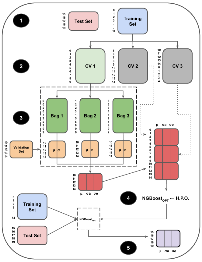
Figure 2: Training pipeline for mirkwood in five sequential steps. Step 1: We divide the input data set $\mathcal{D}$ into $N_{\rm CV,1}=4$ cross-validation folds, at any point referring to the collation of $N_{\rm CV,1}-1$ of them as $\mathcal{D_{TRAIN}}$, and the remaining fold as $\mathcal{D_{TEST}}$. We repeat this $N_{\rm CV,1}$ times to cover all samples in $\mathcal{D}$, but depict only one such iteration here for illustration. Step 2: We sub-divide $\mathcal{D_{TRAIN}}$ into $N_{\rm CV,2}=3$ CV folds. Same as before, $N_{\rm CV,2}-1$ folds are collated while the remaining fold, referred to as the validation set $\mathcal{V}$, is set aside. Step 3: Each of the $N_{\rm CV,2}$ CV folds is used to create $N_{\rm bags}=3$ ‘bags’ by randomly shuffling its data and picking the same number of samples with replacement. An NGBoost model with a given set of hyperparameters is copied over $N_{\rm bags}$ times, and each copy is trained on one ‘bag’ of data. The predictions of all $N_{\rm bags}$ models on $\mathcal{V}$ are recorded and averaged according to Equation 1 to obtain the mean, epistemic, and aleatoric uncertainties for $\mathcal{V}$. Step 4: This process is repeated 100 times to find better performing hyperparameters for NGBoost; we refer to thus optimized model as NGBoost_OPT. Step 5: Finally, we train NGBoost_OPT on $\mathcal{D_{TRAIN}}$ and predict the output for $\mathcal{D_{TEST}}$.

3.1 Uncertainty Quantification

Real observations differ from simulations in a number of ways.

• It is rarely the case that observers have access to all filters in a survey for every observed galaxy. For example, one might encounter a situation where they are interested in determining a galaxy’s mass from its photometry, but do not have access to $K$ and $H$ band information, thus making their task difficult.

• Different filters have differing sensitivities and noise properties, resulting in non-uniform measurement noises across observation bands. Even in an ideal case where observations in UV, optical and IR are equally robust, there is an irreducible Poisson measurement error.

• While modern hydrodynamical simulations have demonstrated a number of successes, there is an inherent, irreducible domain gap between their approximation of reality, and actual reality. Imperfect modeling assumptions both about known physical processes, and arising from our sheer lack of knowledge of them, are primary contributors to this gap. Some specific reasons are modeling star formation with a sub-resolution model, divergence of modeled stellar mass functions from observed ones, and incomplete understanding of AGN feedback processes.

• Any supervised ML algorithm is only as good as the data on which it is trained. It might well be the case that an observed galaxy is in a completely different parameter space than any of the galaxies in our training set.

• Even if some particular model, say NGBoost, with a given set of hyperparameters, is able to faithfully and satisfactorily predict galaxy properties, it is very well possible that there exist other models which can also make predictions that are just as accurate. It is also possible that for our chosen model/set of models, a different data pre-processing scheme, choice of hyperparameters (as mentioned in Section 3, the chosen set of hyperparameters is locally optimal but is not guaranteed to be globally optimal), or choice of scheme for balancing classes might result in better predictions.

Owing to these factors, a highly desirable behavior of any predictive model would be to not only return a point prediction (per galaxy property under consideration), but also some quantity conveying the model’s belief or confidence in its output (Kendall & Gal, 2017; Choi et al., 2018). We can break down such predictive uncertainty into two parts–aleatoric and epistemic Kendall & Gal (2017). Aleatoric uncertainty captures the uncertainty in the data generating process – for example, measurement noise in filters, or the inherent randomness of a coin flipping experiment. It cannot be reduced by collecting more training data; however, it can be reduced by collecting more informative features. On the other hand, epistemic uncertainty models the ignorance of the predictive model, and can indeed be explained away given a sufficiently large training dataset. Aleatoric uncertainty is thus irreducible or statistical, epistemic being its reducible or systematic cousin. Aleatoric uncertainty covers first three of the five issues above, while epistemic uncertainty subsumes the last two points. High aleatoric uncertainty can be indicative of noisy measurements or missing informative features, while high epistemic uncertainty could be a clue that the observed galaxy is very different that any of the galaxies the model was trained on (such a galaxy is referred to as being out of distribution).

As previously discussed, the aim for a supervised ML algorithm is to learn the latent data generating mechanism that maps each input sample $\mathbf{x}_{i}$ to its corresponding output label $y_{i}$. This can be represented as follows:

$$y_{i}=f(\mathbf{x}_{i})+\eta_{i}$$

where $f(\cdot)$ is the unknown latent function and a measurement error $\eta$ follows a standard normal distributions distribution with a variance $\sigma_{\eta,i}^{2},$ i.e., $\eta_{i}\sim\mathcal{N}\left(\mu=0,\sigma_{\eta,i}^{2}\right)$. The variance of $\eta_{i}$ corresponds to the aleatoric uncertainty, i.e., $\sigma_{\eta,i}^{2}=\sigma_{a,i}^{2}$ where we will denote $\sigma_{a,i}^{2}$ as aleatoric uncertainty associated with the observation $\mathbf{x}_{i}$. Similarly, epistemic uncertainty will be denoted as $\sigma_{e,i}^{2}$. Since $f(\cdot)$ is unknown, by training on the training set the model attempts to approximate, or guess, this function as closely as possible. Suppose that we train $\hat{f}(\mathbf{x})$ to approximate $f(\mathbf{x})$ from the samples in the input data set, $\mathcal{D}$. Then, we can see that

$$\mathbb{E}\|y_{i}-\hat{f}(\mathbf{x}_{i})\|^{2} =\mathbb{E}\|y_{i}-f(\mathbf{x}_{i})+f(\mathbf{x}_{i})-\hat{f}(\mathbf{x}_{i})\|^{2}$$

$$=\mathbb{E}\|y_{i}-f(\mathbf{x}_{i})\|^{2}+\mathbb{E}\|f(\mathbf{x}_{i})-\hat{f}(\mathbf{x}_{i})\|^{2}$$

$$=\sigma_{a,i}^{2}+\sigma_{e,i}^{2},$$

where $\mathbb{E}\|\cdot\|$ is the expectation operator. This indicates the total predictive variance is the sum of aleatoric uncertainty and epistemic uncertainty.

The NGBoost algorithm that forms the backbone of mirkwood is naturally able to output both the mean $\mu_{i}$ and the aleatoric uncertainty $\sigma_{a,i}^{2}$ for a given observation $\mathbf{x}_{i}$. To obtain the epistemic uncertainty $\sigma_{e,i}^{2}$, we use bootstrapping. This involves creating multiples copies of the same training dataset, each time picking samples with replacement, training the same model on all copies, and averaging the results. The goal is to simulate a scenario where a model only has access to limited samples – and hence limited parameter space – and to study how this impacts its predictive ability (see Figure 2, especially Step 3). That is, given an NGBoost model, the predicted label for an observation $\mathbf{x}_{i}$ is represented as:

$$p(\mathbf{y}\mid\mathbf{x}_{i}) =\mathcal{N}\left(\mu_{i},\sigma_{a,i}^{2}\right),$$

Creating $N_{\rm bags}$ bootstrapped bags essentially creates $N_{\rm bags}$ copies of the above equation. To obtain final summary statistics, we combine them as

$$\hat{\mu}_{i}{=}\sum_{j=1}^{N_{\rm bags}}\mu_{i,j};\;\hat{\sigma}_{i,a}^{2}{=}\sum_{j=1}^{N_{\rm bags}}\sigma_{i,a,j}^{2};\;\hat{\sigma}_{i,e}^{2}{=}\sum_{j=1}^{N_{\rm bags}}(\mu_{i,j}{-}\hat{\mu}_{i})^{2}$$ (1)

The upshot of this exercise is that the errors modeled by mirkwood encapsulates both the propagated noise due in the input samples, and the uncertainty arising due to the finite size of the training set. The inclusion of the latter source of uncertainty represents a significant advancement over the current state-of-the-art (e.g. Lovell et al., 2019; Acquaviva et al., 2015), and helps mitigate the over-confidence in predictions that is typical of machine learning models.

Table 3: Summary of machine learning terms and variables appearing in this work.

Term	Meaning
Bagging	Bootstrapped Aggregation. A technique of building several models at a time by randomly sampling with replacement, or bootstrapping, from the original data set. Each bag may or may not be the same size as the parent training data set.
HPO	Hyperparameter optimization. The task of finding a well performing set of hyperparameters for any given ML algorithm.
Chaining	Given multiple outputs of interest (dependent variables), the technique of running the regression model in sequence to exploit correlations among them.
Cross validation	The task of dividing the training set into non-overlapping ‘folds’ for the purpose of hyperparameter optimization.
$\mathcal{D}$	Input training set comprising of all samples from Simba, Eagle, and IllustrisTNG. Each sample consists of input (independent variables)-output(dependent variables) pairs.
$\mathcal{D_{TRAIN}}$	Training set, derived from $\mathcal{D}$. mirkwood is trained on this, and used for inference on $\mathcal{D_{TEST}}$.
$\mathcal{D_{TRAIN_{TRAIN}}}$	Training set, derived from $\mathcal{D_{TRAIN}}$. Used for HPO.
$\mathcal{D_{TRAIN_{VAL}}}$	Validation set, derived from $\mathcal{D_{TRAIN}}$. Used for HPO.
$\mathcal{D_{TEST}}$	Test set.
$N_{\rm{CV,1}}$	Number of CV folds that is used to produce $\mathcal{D_{TRAIN}}$ and $\mathcal{D_{TEST}}$ from $\mathcal{D}$.
$N_{\rm{CV,2}}$	Number of CV folds that is used to produce $\mathcal{D_{TRAIN_{TRAIN}}}$ and $\mathcal{D_{TRAIN_{VAL}}}$ from $\mathcal{D_{TRAIN}}$.
$\sigma_{e}$	Epistemic uncertainty.
$\sigma_{a}$	Aleatoric uncertainty.
$f(\cdot)$	Functional representation of mirkwood. This acts on a given input vector $\mathbf{x}$ to produce the output $y$.
$\mu$	The mean of a predicted galaxy property, using one bag of training data.
$\hat{\mu}$	The mean of $\mu$s predicted by all $N_{\rm{bags}}$ bags.

3.2 Performance Metrics

As we have discussed, for each input sample mirkwood outputs three values: $\mu$, $\sigma_{a}$, and $\sigma_{e}$. As the same time, for each input, Prospector outputs two values: $\mu$, and $\sigma$. We quantify the performance of each model by comparing the predicted galaxy properties against the true ones known from simulations. We divide this task into two parts – comparing just the predicted mean deterministic predictions of each galaxy property with its ground truth value, and judging the quality of the entire predicted PDF (probability distribution function; probabilistic predictions) by comparing it against the ground truth value.

3.2.1 Metrics for Deterministic Predictions

For determining the ‘goodness’ of the predicted means for the galaxy properties, we adopt the following three performance criteria:

• Normalized root-mean-square error (RMSE):

  $$\mathrm{NRMSE}=\sqrt{\frac{1}{n}\sum_{i=1}^{n}\left(\hat{\mu}(i)-Y(i)\right)^{2}}$$

• Normalized mean absolute error (NMAE):

  $$\mathrm{NMAE}=\frac{1}{n}\sum_{i=1}^{n}\left|\hat{\mu}(i)-Y(i)\right|$$

• Normalized bias error:

  $$\mathrm{NBE}=\frac{1}{n}\sum_{i=1}^{n}\hat{\mu}(i)-Y(i)$$

where $Y(i)$ and $\hat{\mu}(i)$ are the true and predicted values of any of the five galaxy properties for the $i^{th}$ sample, while $n$ is the total number of samples. A perfect prediction would result in NRMSE, NMAE, and NBE of 0. These values can be seen in the top-left plots in Figures 4 through 7.

3.2.2 Metrics for Probabilistic Predictions

Probabilistic predictions are assessed by constructing Confidence Intervals (CI) and using them in evaluation criteria. In this work, we adopt average coverage area (ACE) and interval sharpness (IS) as our metrics. $\alpha$ is the significance level – the probability that one will mistakenly reject the null hypothesis when in fact it is true. Specifically, since in this paper we are interested in $+/-1\sigma$ predictions (CI=68.2%), we choose $\alpha=1-\rm{CI}=0.318$. For mirkwood results, $\sigma=\sqrt{\sigma_{a}^{2}+\sigma_{e}^{2}}$, while for Prospector results, there is only one $\sigma$ per prediction. For a given sample $i$, if the prediction of any galaxy property, from either mirkwood or Prospector, is {$\mu(i)$; $\sigma(i)$}, then the lower and upper confidence intervals $L_{\alpha}(i)$ and $U_{\alpha}(i)$ are given by $\mu(i)-\sigma(i)$ and $\mu(i)+\sigma(i)$, respectively. $l_{\alpha}(i)$ and $u_{\alpha}(i)$ correspond to the $u-$values for these: $l_{\alpha}(i)=0.5-\rm{CI}/2=0.159$, $u_{\alpha}(i)=0.5+\rm{CI}/2=0.841$. $y(i)$ corresponds to the $u-$value of the ground truth value $Y(i)$. If the predicted mean $\hat{\mu}(i)$ for a galaxy property exactly matches $Y(i)$, then $y_{\alpha}(i)=0.5$; if the predicted mean overshoots or undershoots the ground truth value, then $y_{\alpha}(i)>0.5$ or $y_{\alpha}(i)<0.5$, respectively.

• Average Coverage Error (ACE):

  $$\mathrm{ACE}_{\alpha}=\frac{1}{n}\sum_{i=1}^{n}c_{\alpha}(i)\times 100\%-100\times(1-\alpha)\%,$$

  where $c_{i}$ is the indicative function of coverage:

  $$c_{\alpha}(i)=\left\{\begin{array}[]{l}1,Y(i)\in\left[L_{\alpha}(i),U_{\alpha}(i)\right]\\ 0,Y(i)\notin\left[L_{\alpha}(i),U_{\alpha}(i)\right]\end{array}\right.$$

  ACE is effectively the ratio of target values falling within the confidence interval to the total number of predicted samples.

• Interval Sharpness (IS):

  $$\mathrm{IS}_{\alpha}=\frac{1}{n}\sum_{t=1}^{n}\left\{\begin{array}[]{ll}-2\alpha\Delta_{\alpha}(i)\\ -4\left[l_{\alpha}(i)-y(i)\right],&y(i)<l_{\alpha}(t)\\ -2\alpha\Delta_{\alpha}(i)\\ -4\left[y(i)-u_{\alpha}(i)\right],&y(i)>u_{\alpha}(t)\\ -2\alpha\Delta_{\alpha}(i),&\mathrm{otherwise}\end{array}\right.$$

  where $\Delta_{\alpha}(i)=u_{\alpha}(i)-l_{\alpha}(i)=0.682$. As a reminder, corresponding to $+/-1\sigma$ intervals, $\alpha=0.318$, $l_{\alpha}(i)=0.159$, and $u_{\alpha}(i)=0.841$.

From the equation of ACE, a value close to zero denotes the high reliability of prediction interval. As an infinitely wide prediction interval is meaningless, IS is another indicator contrary to the coverage rate of interval, which measures the accuracy of probabilistic forecasting. $\mathrm{IS}_{\alpha}$ is always $<0$; a great prediction interval obtains high reliability with a narrow width, which has a small absolute value of IS.

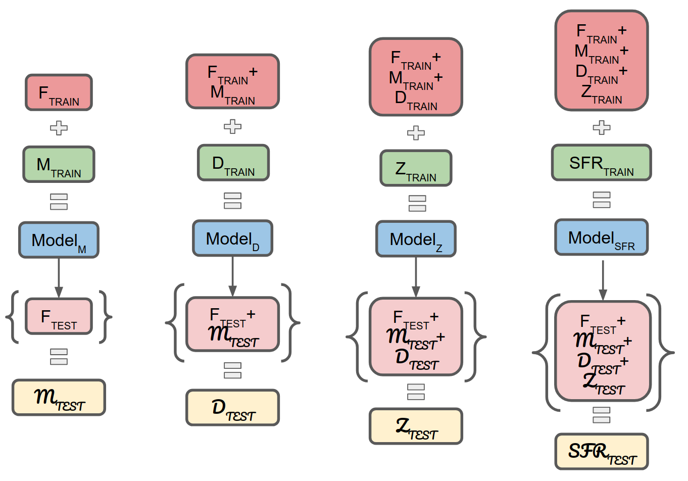
Figure 3: Chained multi-output regression. From left to right, we train models to sequentially predict galaxy stellar mass, dust mass, stellar metallicity, and SFR₁₀₀. At the first step, we train mirkwood on fluxes (as input) and stellar mass (as output) in the training set $\mathcal{D_{TRAIN}}$, and use it to predict stellar mass for samples in the test set ($\mathcal{D_{TEST}}$) using their respective flux values as inputs. In the second step, we append the true stellar masses of samples in $\mathcal{D_{TRAIN}}$ with their fluxes, and append the predicted stellar masses of the samples in $\mathcal{D_{TEST}}$ to theirs. A new model is then trained on the extended training set, and used to predict dust mass mass for samples in the test set. We continue thus until all five properties have been successfully predicted for all samples in the original $\mathcal{D_{TEST}}$.

4 Results

Figure 4: Comparison of predicted v/s true stellar mass – in terms of both means and uncertainties – for samples from the Simba simulation. (a), (c) Predicted mean stellar mass from mirkwood v/s Prospector: We can see both qualitatively and quantitatively (via the three metrics normalized root mean square error, normalized mean absolute error, and normalized bias error) that predictions from mirkwood are a significant step-up from traditional SED-based results. As a reminder, the smaller the three metrics, the better the predictions. For clearer visualization, we have used scatter points for results from mirkwood, and contour lines for results from Prospector. In subplot (c), we employ histograms to demonstrate the radically different bias and variance in predictions from the two models. (b) Predicted aleatoric uncertainty in stellar mass from mirkwood v/s Prospector: We compare the predicted aleatoric uncertainty from mirkwood with the aleatoric uncertainty from traditional SED fitting. Both qualitatively and quantitatively – by employing the metrics average coverage error, and interval sharpness – we see that predictions from mirkwood are superior. As explained in Section 3.2.2, these probabilistic metrics such as ACE and IS are essential to evaluate predicted uncertainties, something that is outside the purview of traditional deterministic metrics such as those used in subplot (a) and expounded upon in Section 3.2.1. (d) Importance of different bands in predicting stellar mass from mirkwood: SHAP values are a way to obtain contribution of each feature (predictive variable) in predicting a model’s output. They measure how reactive the output is to changes in the input, and thus they can be thought of as a type of sensitivity measure; see Section 4 and Appendix A for detailed discussion. Here we see that K and H bands are the most important predictors of stellar mass, with higher flux values (red color) corresponding to higher mass values.

Figure 5: Very similar to Figure 4, this figure compares predicted v/s true dust mass – in terms of both means and uncertainties – for samples from the Simba simulation. (a), (c) Predicted dust mass from mirkwood v/s Prospector: Just like in Figure 4, we see that predictions from mirkwood are a significant step-up from traditional SED-based results. (b) Predicted aleatoric uncertainty in dist mass from mirkwood: Unlike in Figure 4, we only plot the calibration curve for aleatoric uncertainties from mirkwood, since in this work we do not have access to uncertainties in dust mass from Prospector. (d) Importance of different bands in predicting dust mass from mirkwood: We see that the NIR bands are the most predictive of dust mass, with only a tiny contribution from predicted mass. This tracks with our understanding of dust mass properties.

Figure 6: Same as Figures 4 and 5, but for instantaneous star formation rate metallicity Z.

Figure 7: Same as Figures 4, 5, and 6 but for instantaneous star formation rate SFR₁₀₀.

In order to test our proposed model for SED fitting, we compare against fits from the Bayesian SED fitting software prospector. prospector and mirkwood are given the same information in order to infer galaxy properties. This includes broadband photometry in $35$ bands with 5%, 10%, and 20% Gaussian uncertainties (respectively SNRs = 20, 10, and 5). We present here the results from both methods for several galaxy properties including stellar mass, dust mass, star formation rate averaged over the last 100 Myr (SFR₁₀₀), and stellar metallicity.

In Figures 4 through 7, we present mirkwood’s predictions when trained on the full dataset comprising of simulations from Simba, Eagle, and IllustrisTNG, for SNR=5. The training set contains all 10,073 samples from IllustrisTNG, 4,697 samples from Eagle, and 359 samples from Simba selected by stratified 5-fold cross-validation (see Section 3 for details on implementation), while the test set contains the remaining 1,438 samples from Simba. After making inference on all test splits, we collate the results, thus successfully predicting all four galaxy properties for all 1,797 samples from Simba. Each predicted output for a physical property contains three values – the mean $\mu$, the aleatoric uncertainty $\sigma_{\rm a}$, and the epistemic uncertainty $\sigma_{\rm e}$. The first type of uncertainty quantifies the inherent noise in the data, while the second quantifies the confidence of the model in the training data (see Section 3.1 for detailed description). The results from traditional SED fitting are a subset of the total training data.We present a brief overview of the data sets in Table 1.

In subplots (a) of Figures 4 through 7, we plot the recovered physical properties from mirkwood and prospector against the true values from the simulations for each of the four modeled properties: stellar mass, dust mass, metallicity, and star formation rate. In each case, the blue contours represent the physical properties derived from traditional SED fitting, while the orange points denote the results from mirkwood. Without exception, mirkwood provides superior predictions, as evidenced both by a visual inspection, and via a more quantitative approach by using three different metrics (detailed in Section 3.2).

In subplots(b), we plot ‘calibration diagrams’ (Zelikman & Healy, 2020). On the y-axis are the inverse-CDFs (cumulative distribution functions) for predictions from both mirkwood and Prospector. These are commonly used in ML literature – the plotting function takes as input a vector consisting of the ground truth value, predicted mean, and predicted standard deviation, and outputs a value between 0 and 1 (see Kuleshov et al. (2018) for detailed instructions on constructing these diagrams). We repeat this for all samples in the test set $\mathcal{D_{TEST}}$, sort the resulting vector in ascending order, and plot the curve on the y-axis. For mirkwood, the uncertainty used is $\sigma_{\rm a}$, while Prospector does not differentiate between the two types of uncertainties and outputs a single value per galaxy sample. A 1:1 line on this curve indicates a perfectly calibrated set of predictions, with deviations farther from it indicative of poorer calibration. Both visually and quantitatively by using the two probabilistic metric (Section 3.2) average coverage error and interval sharpness, we ascertain that mirkwood outperforms traditional SED fitting.

In subplots (c) and (d), we plot the histograms for predicted means, and SHAP summary plots for samples in $\mathcal{D_{TEST}}$, respectively. The histograms in subpolots (c) enable us to visualize both bias and variance in predictions from mirkwood, and compare the results to those from Prospector. As is readily apparent, both these quantities are significantly smaller for predictions from our ML-based model than from traditional SED fitting, for all four galaxy properties. We explain in detail how SHAP values are calculated in Section A. In brief, for a given filter (dotted vertical lines in subplots (d)), an absolute value farther from 0 denotes a larger impact of that feature in affecting the model outcome. SHAP values can thus be thought of as a type of sensitivity – it controls how reactive the output is to changes in the input (here flux in the filter). Red and blue indicate high and low ends of values per feature/filter. Thus for a given feature, SHAP values $>0$ with a red hue indicate that the galaxy property increases as that feature increases. Similarly, SHAP values $>0$ with a blue hue indicate that the galaxy property decreases as the feature value decreases. As an example, in panel (d) of Figure 4, the largest correlations with the $M^{\star}$ of a galaxy are, quite naturally, the $\sim 1-2\mu$m range.

In Table 4, we delineate all five metrics from Section 3.2 to quantitatively compare mirkwood’s performance with that of traditional SED fitting, across different levels of noise. As we would expect, the results from both models improve with increasing SNR. Across every metric and galaxy property, mirkwood demonstrates excellent performance. We also note that the difference in their relative performances increases with increasing noise level. Below a certain SNR, traditional SED fitting stops producing meaningful results (as can also be seen clearly from subplots (a) in Figures 4 through 7 ), whereas our ML-based approach is still able to extract signal from the noisy data.

Finally, in Figures 8 through 11, we demonstrate the impact of different training sets on predictions from mirkwood, for all three SNRs of 5, 10, and 20. In all figures, ‘P’ stands for results from Prospector, ‘SET’ for results from mirkwood when the training dataset contains samples from IllustrisTNG, Eagle, and Simba, ‘ET’ for Eagle and IllustrisTNG, ‘T’ for only IllustrisTNG, ‘E’ for only Eagle, and ‘S’ for only Simba. For ‘SET’ and ‘S’, we use stratified 5-fold cross validation to select non-overlapping samples from Simba in the training set. As expected, we obtain the best predictions, as quantified by various deterministic and probabilistic metrics, when the training set consists of samples from all three simulations. This ensures the most diverse coverage in parameter space, and hence offers the highest generalization power. We also notice that prediction quality improves as the SNR improves, something that one would intuitively expect.

Figure 8: Impact of training set on mirkwood’s performance on predicting galactic stellar mass: Using the three deterministic metrics and two probabilistic metrics introduced in 3.2, we evaluate the impact that different training sets have on predictions of stellar mass from mirkwood on galaxy samples from Simba. ‘P’ stands for results from prospector (traditional SED fitting), ‘SET’ for training set consisting of all Simba, Eagle, and IllustrisTNG, and so on. The test set is always Simba. We separate the aleatoric error from the epistemic uncertainty to provide a more granular visualization. As is apparent, at all noise levels, mirkwood outperforms traditional SED fitting. Aleatoric uncertainty is generally the lowest when the training set is as diverse as possible, while epistemic uncertainty is always the lowest when the training set samples are drawn from the same simulation as the test set samples (Simba).

Figure 9: Same as Figure 8, but for dust mass.

Figure 10: Same as Figures 8 and 9, but for metallicity Z.

Figure 11: Same as Figures 8, 9 and 10 but for instantaneous star formation rate SFR₁₀₀.

5 Discussion and Future Work

Our work shows that it is possible to reproduce galaxy property measurements with high accuracy in a purely data-driven way by using robust ML algorithms that do not have any knowledge about the physics of galaxy formation or evolution. The biggest caveat here is that the training set must be closely representative of the data of interest, i.e. observations of real galaxies. We also demonstrate the necessity of carefully accounting for both the noise in the data and sparsity of the training set in any given parameter-space of interest. By combining galaxy simulations with disparate physics, we offer a way to better train our model for a real observation. Across all SNRs, we show a considerable improvement over state-of-the-art SED fitting using Prospector and non-parametric SFH model, both in terms of prediction quality and compute requirements. For comparison, mirkwood ran for $\sim$ 24 hours on the first author’s home workstation with 12 cores, to derive all four galaxy parameters for $\sim$ 1700 SIMBA galaxies; prospector required about the same time, but 3,000 cores on the University of Florida HiPerGator supercomputing system. Another notable result is that we are able to extract accurate galaxy properties from photometries with SNRs as low as 5. All these contributions considered together imply that scientifically interesting galaxy properties can be accurately and quickly measured on future datasets from large-scale photometric surveys.

Several avenues for future research remain open. The crux of our follow-up efforts will focus on development of mirkwood to a higher level of complexity and precision. We identify the following areas for improvement:

1. Extensive hyperparameter optimization: In this work we use NGBoost models with hyperparameters only slightly modified from the prescription of Ren et al. (2019). This is an easy avenue for gaining performance boost with respect to reconstruction of galaxy properties – in future work we will leverage modern Bayesian hyperparameter optimization libraries to conduct extensive HPO to eke out maximum performance from our models.

2. Managing missing observations: Most real-life observations of all galaxies do not contain observations in the same set of filters, nor is the SNR of the data in each filter the same. Currently, mirkwood cannot easily accommodate these complications, since NGBoost is unable to natively handle missing feature values. In future work we will explore other boosted tree models, such as CatBoost (Prokhorenkova et al., 2018), to extract galactic properties from real observations.

3. Synergistic spectroscopy: While spectroscopic data are considerably more expensive to obtain, there exist targets where photometry and spectra are available simultaneously (Carnall et al., 2019). Modeling both modes of data simultaneously can increase the SNR available to any model, and help significantly in reducing uncertainties in derived galaxy properties, thus enabling accurate re-construction of higher resolution ones such as a galaxy’s entire star formation history. We will explore inclusion of a convolutional neural network to this end, similar to the work of Lovell et al. (2019).

4. Probability calibration: This is a post-processing step that has been shown to improve predictions, measured both by deterministic and probabilistic metrics. ML algorithms are often over-confident, and unable to assess the degree of their fallacy – if given a completely novel input, most commonly used ML algorithms are likely to predict a wrong label for it, instead of just saying, ‘I do not know the correct answer.’ Probability calibration is widely used in the machine learning community (Nixon et al., 2019; Kuleshov et al., 2018; Zelikman & Healy, 2020; Lakshminarayanan et al., 2017), albeit its adoption in astronomy has been slow. We expect probability calibration would result in more sensible uncertainties in the second through fourth columns of Figures 8 through 11. Specifically, we expect that calibrated aleatoric, epistemic, and total uncertainties would mean the lowest ACE and IS values for the ‘SET’ column, which is not consistently the case in this paper.

5. Randomized chaining: Here we have considered one particular way of chaining galaxy properties: only fluxes are used when predicting stellar mass, fluxes and predicted stellar mass are synergistically used to predict dust mass, and so on all the way till SFR₁₀₀ (see Figure 3 for details). However, given the interdependence of all properties, a more justified approach would be to consider multiple such orderings and average the result. For instance, to predict stellar mass, $\rm{model}_{1}$ will be trained on just the galaxy fluxes, $\rm{model}_{2}$ on fluxes + metallicity, $\rm{model}_{3}$ on fluxes + dust mass + SFR₁₀₀, and all such permutations. Finally, the predicted stellar mass results will be averaged. We expect this would average out any biases introduced by chaining in any particular order, and we plan to explore this line of research in more detail.

6. Redshifts as both input and output: We plan on expanding the training set considerably by incorporating photometries from galaxies a range of redshifts to enable extraction of properties of real galaxies. In this sense, redshift would be the fifth output variable. On the other hand, it might very well be the case that for a given set of samples, high-confidence spectroscopic redshift is available, but photometry data is present only in a few bands. In such a case, it would be sensible to use redshift as an input rather than an output. We plan on upgrading our network so that mirkwood can easily take a redshift as either a fixed input, or take a user-given prior for redshift which it will then aim to improve.

7. Semi-supervised learning: In an effort to reduce the ‘domain gap’ – the difference between the training set(s) and real life data – several semi-supervised algorithms have been developed and used. These can smoothly combine a computer simulated set of data with high-confidence real life-observations, such as spectra, to more closely approximate reality.

8. Outlier detection and elimination: In its current implementation, mirkwood is unable to identify and reject outlying inputs. These can result from any of the several data processing pipelines that are used to create scientifically interesting data products can fail and output nonsensical numbers, for example a flux absurdly high as $10^{252}$. This issue becomes even more urgent when dealing with semi-supervised learning, where data from real-life observations form part of the training set. In future we plan on exploring algorithms such as variational auto-encoders (Ghosh & Basu, 2016; Zellner, 1988; Gilda et al., 2020) to this end.

5.1 On SED Modeling Priors and Assumptions

A fundamental aspect of SED modeling is the choice of model for each component (e.g. SFH or dust attenuation) and the subsequent priors used to constrain the models. In this work, we have used prospector to fit the synthetic SEDs of galaxies from three cosmological simulations, following the model assumptions outlined in Lower et al. (2020). There, the model components, namely the non-parametric SFH, were optimized to result in the best possible estimates for stellar mass, mass-weighted stellar age, and recent SFR for the simba simulation at $z=0$. However, it is conceivable that these optimizations do not hold true for eagle or illustris TNG. For instance, in recent work by Iyer et al. (2020), the above cosmological simulations produce significantly different SFHs depending on the different subgrid models for, e.g., star formation and stellar feedback, which modulate the short and long-timescale variations of a galaxy’s SFH. Thus, using the same SFH model to describe the galaxy SFHs from these simulations may not be justified, but is ultimately outside the scope of this paper to fully tune the SFH models for each simulation. Similarly, in future work, we are working to implement physically motivated priors to further improve the results from traditional SED fitting by including variable dust attenuation curves.

One advantage of mirkwood in this regard is the freedom from choosing a particular SFH model, dust attenuation law, or set of priors to infer galaxy properties from broadband photometry. Combining the input from three cosmological simulations as a training set for mirkwood removes the simplifications of modeling galaxy SEDs with relatively simple analytic functions as in traditional SED modeling. This method of inferring galaxy properties can also overcome the biases that affect traditional SED fitting, such as the outshining of older stellar populations by younger, massive stars which generally causes stellar masses to be under-estimated for star forming galaxies (Papovich et al., 2001) and the generally poor reconstruction of early SFHs due to the non-uniform sensitivity to variations in star formation as a function of time (i.e.that SED fitting is more sensitive to recent star formation and much information about star formation beyond a few Gyr before the observation is lost) (Iyer et al., 2019).

5.2 Caveats to the Mirkwood Training Set

Though mirkwood is trained on a wealth of data from three moderate volume cosmological simulations, we are not yet free from broad assumptions pertaining to stellar population synthesis modeling. mirkwood relies on synthetic galaxy SEDs generated by post-process 3D dust radiative transfer modeling via hyperion and fsps. In practice, we have assumed a universal initial mass function (IMF) for all galaxies as well as one library of stellar spectra and isochrones. Although this method is similar to traditional SED fitting, our training set is tied to these particular models. To understand the magnitude of importance of these assumptions on inferring galaxy properties, we would need to regenerate the synthetic galaxy SEDs for each combination of IMFs, spectral libraries, and isochrones, representing millions of hours of CPU time in addition to the time required to retrain mirkwood on each set of SEDs for each redshift. Given the scale this problem requires, this retraining is ultimately outside the scope of this work.

Table 4: Comparative performance of mirkwood v/s Prospector across different noise regimes. The five metrics are the normalized root mean squared error (NRMSE), normalized mean absolute error (NMAE), normalized bias error (NBE), average coverage error (ACE), and interval sharpness (IS). In any given cell, the tuple of values consists of the metric of interest from mirkwood and Prospector, respectively. A value of ‘nan’ represents lack of predictions from Prospector. We do not have predicted error bars from Prospector for dust mass, hence ACE and IS values corresponding to this property are ‘nan’s.

	SNR	NRMSE	NMAE	NBE	ACE	IS
	5	(0.198, 1.003)	(0.123, 1.091)	(-0.042, -0.528)	(-0.002, -0.497)	(0.001, 0.005)
Mass	10	(0.165, 1.0)	(0.118, 1.088)	(-0.035, -0.518)	(-0.021, -0.502)	(0.001, 0.004)
	20	(0.155, 1.002)	(0.115, 1.117)	(-0.041, -0.479)	(-0.066, -0.482)	(0.001, 0.033)
	5	(0.48, 0.996)	(0.339, 0.998)	(-0.219, -0.905)	(0.003, nan)	(0.001, nan)
Dust Mass	10	(0.456, 0.996)	(0.332, 0.998)	(-0.209, -0.905)	(-0.033, nan)	(0.001, nan)
	20	(0.475, 1.263)	(0.336, 1.212)	(-0.215, -0.679)	(-0.076, nan)	(0.001, nan)
	5	(0.062, 0.544)	(0.06, 0.478)	(-0.011, -0.297)	(-0.024, 0.046)	(0.041, 0.301)
Metallicity	10	(0.058, 0.534)	(0.055, 0.464)	(-0.01, -0.275)	(-0.032, 0.041)	(0.036, 0.295)
	20	(0.056, 0.547)	(0.052, 0.487)	(-0.01, -0.229)	(-0.063, 0.036)	(0.032, 0.302)
	5	(0.241, 0.907)	(0.205, 0.99)	(-0.069, -0.687)	(0.074, -0.557)	(7.314, 0.001)
SFR	10	(0.329, 0.91)	(0.226, 0.992)	(-0.09, -0.686)	(0.048, -0.564)	(1.937, 0.001)
	20	(0.277, 1.988)	(0.215, 2.911)	(-0.078, 1.437)	(0.035, -0.547)	(0.006, 0.2)

Appendix A Shapley Values

Consider a dataset X with $N$ features and $S$ samples $\textbf{X}=\left\{X^{(1)}_{1:S},\ldots,X^{(N)}_{1:S}\right\},$ and a continuous, real-valued target variable vector $Y_{1:S}$. Given an instance (observation) $x\in\textbf{X}\in\textsc{R}^{1:N},$ a model $v$ forecasts the target as $v(x)$. In addition to this forecasting, we would also like to know if we can attribute the departure of the prediction $v(x)$ from the average value of the target variable $\bar{y}=\bar{Y}_{1:S}$ to each of the features (predictor variables) in the observed instance $x$? In a linear model, the answer is trivial :$v(x)-\bar{y}=\beta_{1}x^{(1)}+\cdots+\beta_{N}x^{(N)}$ (see Slide 13 in López de Prado 2020). We would like to do a similar local decomposition for any (non-linear) ML model. Shapley values answer this attribution problem through game theory (Shapley, 1953). Specifically, they originated with the purpose of resolving the following scenario–a group of differently skilled participants are all cooperating with each other for a collective reward; how should this reward be fairly divided amongst the group? In the context of machine learning, the participants are the features of our input dataset X and the collective payout is the excess model prediction (i.e., $v(x)-\bar{y}$). Here, we use Shapley values to calculate how much each individual feature marginally contributes to the model output–both for the dataset as a whole (global explainability) and for each instance (local explainability).

While a goal of this paper is to explain the contributions of narrow- and broad-bands to various galaxy properties, for the sake of simplicity we chose to explain Shapley values using a toy example. Let us say that we operate a small hedge fund, and our team consists of three people: Alice, Bob, and Carol. On average, they manage to make approximately $100,000 everyday ($\bar{y}=100$ (thousand)). At the end of the year, we would like to distribute bonuses to our team members in direct proportion to their contribution to beating the average daily profit. Let us consider one day in particular, when owing partly to market volatility and partly to luck, today they make $120,000 (i.e., excess income = 20 (thousand) dollars). Below, we delineate the process of determining each person’s fair contribution to this number.

1. First, we consider the $2^{N=3}$ possible coalitions (interactions) between the players (features), where some players may not participate (i.e., remain at their average value), and other may participate (depart from their average value). See Table 5.

2. Second, we use the coalitions table to compute the marginal contribution of each player conditional on the contribution of every other player. The marginal impact of changing A after changing B may differ from the marginal impact of changing B after changing A. Accordingly, we must account for all possible $N!=6$ sequences of conditional effects. See Table 6.

3. Finally, the Shapley value of a player is calculated as the average conditional marginal contribution of that player across all the possible $N!$ ways of conditioning the predictive model $v$. See last row of Table 6 and Equation A1.

$\text{Alice}\neq\overline{\text{Alice}}$	$\text{Bob}\neq\overline{\text{Bob}}$	$\text{Carol}\neq\overline{\text{Carol}}$	$v(...)\left(=v[x\mid\ldots]\right)-\bar{y}$
0	0	0	$v(\varnothing)(=v[x\mid 000])-\bar{y}=0$
0	0	1	$v(C)(=v[x\mid 001])-\bar{y}=10$
0	1	0	$v(B)(=v[x\mid 010])-\bar{y}=5$
0	1	1	$v(B,C)(=v[x\mid 011])-\bar{y}=7$
1	0	0	$v(A)(=v[x\mid 100])-\bar{y}=2$
1	0	1	$v(A,C)(=v[x\mid 101])-\bar{y}=8$
1	1	0	$v(A,B)(=v[x\mid 110])-\bar{y}=10$
1	1	1	$v(A,B,C)(=v[x\mid 111])-\bar{y}={\color[rgb]{1,.5,0}20}$

Table 5: In a model with 3 features, there are $2^{3}=8$ possible interactions. For each interaction, we compute the departure of the model’s forecast from its baseline (average value). We encode as ‘1’ a feature that is not at its average value (it forms part of a coalition), and ‘0’ a feature that is at its average value. Thus $v(A,B)=v(B,A)$, $v(B,C)=v(C,A)$, $v(A,C)=v(C,A)$, and $v(A,B,C)=v(B,A,C)=v(A,C,B)$.

Combination	Alice	Bob	Carol	Total
$\mathrm{A},\mathrm{B},\mathrm{C}$	$v(\mathrm{A})-v(\varnothing)=2$	$v(\mathrm{A},\mathrm{B})-v(\mathrm{A})=8$	$v(\mathrm{A},\mathrm{B},\mathrm{C})-v(\mathrm{A},\mathrm{B})=10$	20
$\mathrm{A},\mathrm{C},\mathrm{B}$	$v(\mathrm{A})-v(\varnothing)=2$	$v(\mathrm{A},\mathrm{C},\mathrm{B})-v(\mathrm{A},\mathrm{C})=12$	$v(\mathrm{A},\mathrm{C})-v(\mathrm{A})=6$	20
$\mathrm{B},\mathrm{A},\mathrm{C}$	$v(\mathrm{B},\mathrm{A})-v(\mathrm{B})=5$	$v(\mathrm{B})-v(\varnothing)=5$	$v(\mathrm{B},\mathrm{A},\mathrm{C})-v(\mathrm{B},\mathrm{A})=10$	20
$\mathrm{B},\mathrm{C},\mathrm{A}$	$v(\mathrm{B},\mathrm{C},\mathrm{A})-v(\mathrm{B},\mathrm{C})=13$	$v(\mathrm{B})-v(\varnothing)=5$	$v(\mathrm{B},\mathrm{C})-v(\mathrm{B})=2$	20
$\mathrm{C},\mathrm{A},\mathrm{B}$	$v(\mathrm{C},\mathrm{A})-v(\mathrm{B})=3$	$v(\mathrm{C},\mathrm{A},\mathrm{B})-v(\mathrm{C},\mathrm{A})=12$	$v(\mathrm{C})-v(\varnothing)=10$	20
$\mathrm{C},\mathrm{B},\mathrm{A}$	$v(\mathrm{C},\mathrm{B},\mathrm{A})-v(\mathrm{C},\mathrm{B})=13$	$v(\mathrm{C},\mathrm{B})-v(\mathrm{C})=-3$	$v(\mathrm{C})-v(\varnothing)=10$	20
Average	$6.3$	$6.5$	$8$	20

Table 6: In a model with 3 features, there are $3!=6$ possible sequences. We can use the interactions table to derive the marginal contribution of each feature in each sequence. The Shapley values are the averages per column.

Eliminating Redundancy: As we can appreciate from the numerical exercise in Tables 5 and 6, some calculations are redundant. For example, the marginal contribution of C on sequence (A, B, C) must be the same as the marginal contribution of C on sequence (B, A, C), because (a) in both cases C comes in third position, and (b) the permutations of (A, B) do not alter that marginal contribution. The Shapley value of a feature $i$ can be derived as the average contribution of $i$ across all possible coalitions $S$, where $S$ does not include feature $i$:

$$\phi_{i}(v)=\sum_{S\subseteq N\backslash\{i\}}\frac{|S|!(|N|-|S|-1)!}{|N|!}(v(S\cup\{i\})-v(S))$$ (A1)

The above equation describes a coalitional game (the scenario described previously) with a set N of $|\textbf{N}|$ players. The function $v$ gives the value (payout) for any subset of those players. For example, if $S$ be a subset of N, then v(S) gives us the value of that subset. Thus for a coalitional game (N, v) Equation A1 outputs the value for feature i, i.e. its the Shapley value. For ease of explanation, we focus our attention on calculating how many of the excess $20$ (thousand) dollars can be attributed to C(arol), i.e. calculating the Shapley value for C. We then examine the various components of Equation A1 and study their significance.

• If we relate this back to the parameters of the Shapley value formula we have N$=\{A,B,C\}$ and $i=C$. The highlighted section in Equation A4 (derived from Equation A1 by re-arranging some terms) says that we need to take our group of people and exclude the person that we are focusing on now. Then, we need to consider all of the possible subsets that can be formed. So if we exclude C from the group we are left with A, B. From this remaining group we can form the following subsets (i.e. these are the sets that S can take on): $\varnothing,A,B,AB$. In total, we can construct four unique subsets from the remaining team members, including the null set.

  $$\phi_{i}(v)=\frac{1}{|N|}\sum_{{\color[rgb]{1,.5,0}S\subseteq N\backslash\{i\}}}\left(\begin{array}[]{c}|N|-1\\ |S|\end{array}\right)^{-1}(v(S\cup\{i\})-v(S))$$ (A4)

• Next, we focus on the highlighted term in Equation A7.

  $$\phi_{i}(v)=\frac{1}{|N|}\sum_{S\subseteq N\backslash\{i\}}\left(\begin{array}[]{c}|N|-1\\ |S|\end{array}\right)^{-1}{\color[rgb]{1,.5,0}(v(S\cup\{i\})-v(S))}$$ (A7)

  This refers to the marginal value of adding player $i$ to the game. Specifically, we want to see the difference in the money earned daily if we add $C$ to each of our four subsets. We denote these four marginal values as: $\Delta v_{C,\varnothing},\Delta v_{AC,A},\Delta v_{BC,B},\Delta v_{ABC,AB}$. Each of these as a different scenario that we need to observe in order to fairly assess how much C contributes to the overall profit. This means that we need to observe how much excess money is produced if everyone is working at their average levels (i.e. the empty set $\varnothing$) and compare it to what happens if we only have C working at above or below-average productivity. We also need to observe how much profit is earned by A and B working simultaneously and compare that to the profit earned by A and B together with C, and so on.

• Next, the summation in the Shapley value equation is telling us that we need to add all them together. However, we also need to scale each marginal value before we do that, which we are provided this prescription by the highlighted part in Equation A10.

  $$\phi_{i}(v)=\frac{1}{|N|}\sum_{S\subseteq N\backslash\{i\}}{\color[rgb]{1,.5,0}\left(\begin{array}[]{c}|N|-1\\ |S|\end{array}\right)^{-1}}(v(S\cup\{i\})-v(S))$$ (A10)

  It calculates how many permutations of each subset size we can have when constructing it out of all remaining team members excluding feature (player) i. In other words, given $\lvert$N$\rvert$-1 features (players), how many groups of size $\lvert$S$\rvert$ can one form with them? We then use this number to divide the marginal contribution of feature (player) $i$ to all groups of size $\lvert$S$\rvert$. For our scenario, we have that $\lvert$N$\rvert$-1 = 2, i.e. these are the remaining team members when we are left with when calculating the Shapley value for C. In our case we will use that part of the equation to calculate how many groups we can form of size 0, 1, and 2, since those are only group sizes we can construct with the remaining players. So, for example, if we have that $\lvert$S$\rvert$ = 1 then we get that we can construct 2 different groups of this size: A and B. This means that we should apply the following scaling factors to each of our 4 marginal values: $1\Delta v_{C,\varnothing},\frac{1}{2}\Delta v_{AC,A},\frac{1}{2}\Delta v_{BC,B},1\Delta v_{ABC,AB}$. By adding this scaling factor we are averaging out the effect that the rest of the team members have for each subset size. This means that we are able to capture the average marginal contribution of C when added to a team of size 0, 1, and 2 regardless of the composition of these teams.

• Next, we focus on the remaining term, highlighted in Equation A13.

  $$\phi_{i}(v)={\color[rgb]{1,.5,0}\frac{1}{|N|}}\sum_{S\subseteq N\backslash\{i\}}\left(\begin{array}[]{c}|N|-1\\ |S|\end{array}\right)^{-1}(v(S\cup\{i\})-v(S))$$ (A13)

  So far we have averaged out the effects of the other team members for each subset size, allowing us to express how much C contributes to groups of size 0, 1, and 2. The final piece of the puzzle is to average out the effect of the group size as well, i.e. how much does C contribute regardless of the size of the team (number of explanatory features in the data set). For our scenario we do this by dividing with 3 since that is the number of different group sizes that we can consider. With this final step, we arrive at the point where can finally compute the Shapley value for C. We have observed how much she marginally contributes to all different coalitions the team that can be formed. We have also averaged out the effects of both team member composition as well as team size which finally allows us to compute the Shapley value for C:

  $$\phi_{C}(v) =\frac{1}{3}\sum\left(1\Delta v_{C,\varnothing},\frac{1}{2}\Delta v_{AC,A},\frac{1}{2}\Delta v_{BC,B},1\Delta v_{ABC,AB}\right)$$

  $$=\frac{1}{3}\sum\left(1\times 10,\frac{1}{2}\times 6,\frac{1}{2}\times 2,1\times 10\right)$$

  $$=8$$ (A14)

  Comparing Equation • ‣ A with the Shapley value for C in the last row of Table 6, we see that they match exactly.

After calculating the Shapley values for the rest of the players, we can then determine their individual contributions to the excess 20 (thousand) dollars earned today, allowing us to fairly divide the bonus amongst all team members:

$$20 =v(\{A,B,C\})$$

$$=\phi_{A}(v)+\phi_{B}(v)+\phi_{C}(v)$$ (A15)

This is also evident from the last row of Table 6, where the Shapley values for A, B, and C add to the total of 20.

Properties: As they apply to local explanations of predictions from machine learning models, Shapley values have some nice uniqueness guarantees (Shapley, 1953). As described above, Shapley values are computed by introducing each feature, one at at time, into a conditional expectation function of the model’s output, $v_{x}(S)\approx E[v(x)|x_{S}]$, and attributing the change produced at each step to the feature that was introduced; then averaging this process over all possible feature orderings. Shapley values are provably the only possible method in the broad class of additive feature attribution methods Lundberg & Lee (2017) that simultaneously satisfy four important properties of fair credit-attribution: efficiency, symmetry, missingness, and additivity.

1. Efficiency/ Local Accuracy: The sum of the Shapley values of all features (players) equals the value of the total coalition. That is, the value of $20$ in the bottom-rightmost corner in Table 5 is the same as the $20$ in the bottom-rightmost cell in Table 6.

2. Missingness: If a feature (player) never adds any marginal value regardless of the coalition, its payoff (Shapley value $\phi_{i}(v)$) is 0. That is, if: $v(S\cup\{i\})=v(S)\forall$ subsets of features S, then $\phi_{i}(f)=0$.

3. Symmetry: All players have a fair chance to join the game. That’s why Table 5 lists all the permutations of the players. If two players always add the same marginal value to any subset to which they are added, their payoff portion should be the same. In other words, $\phi_{i}=\phi_{j}$ IIF feature i and feature j contribute equally to all possible coalitions.

4. Additivity: A function with combined outputs has as Shapley values the sum of the constituent ones. For any pair of games $v,w$, $\phi(v+w)=\phi(v)+\phi(w)$, where $(v+w)(S)=v(S)+w(S)\forall S$. This property allows us to combine Shapley values from $n$ different models, thus enabling interpretability for ensembles.

References

- Acquaviva et al. (2015) Acquaviva, V., Raichoor, A., & Gawiser, E. 2015, The Astrophysical Journal, 804, 8
- Anglés-Alcázar et al. (2017) Anglés-Alcázar, D., Faucher-Giguère, C.-A., Quataert, E., et al. 2017, MNRAS, 472, L109, doi: 10.1093/mnrasl/slx161
- Barchi et al. (2020) Barchi, P., de Carvalho, R., Rosa, R., et al. 2020, Astronomy and Computing, 30, 100334
- Baron (2019) Baron, D. 2019, arXiv preprint arXiv:1904.07248
- Behroozi et al. (2013) Behroozi, P. S., Wechsler, R. H., & Conroy, C. 2013, The Astrophysical Journal, 770, 57
- Boquien et al. (2019) Boquien, M., Burgarella, D., Roehlly, Y., et al. 2019, Astronomy & Astrophysics, 622, A103
- Breiman (2001) Breiman, L. 2001, Machine learning, 45, 5
- Carnall et al. (2018) Carnall, A., McLure, R., Dunlop, J., & Davé, R. 2018, Monthly Notices of the Royal Astronomical Society, 480, 4379
- Carnall et al. (2019) Carnall, A., McLure, R., Dunlop, J., et al. 2019, Monthly Notices of the Royal Astronomical Society, 490, 417
- Chen & Guestrin (2016) Chen, T., & Guestrin, C. 2016, in Proceedings of the 22nd acm sigkdd international conference on knowledge discovery and data mining, 785–794
- Cheng et al. (2020a) Cheng, T.-Y., Huertas-Company, M., Conselice, C. J., et al. 2020a, arXiv preprint arXiv:2009.11932
- Cheng et al. (2020b) Cheng, T.-Y., Conselice, C. J., Aragón-Salamanca, A., et al. 2020b, Monthly Notices of the Royal Astronomical Society, 493, 4209
- Choi et al. (2016) Choi, J., Dotter, A., Conroy, C., et al. 2016, ApJ, 823, 102, doi: 10.3847/0004-637X/823/2/102
- Choi et al. (2018) Choi, S., Lee, K., Lim, S., & Oh, S. 2018, in 2018 IEEE International Conference on Robotics and Automation (ICRA), IEEE, 6915–6922
- Ciesla et al. (2017) Ciesla, L., Elbaz, D., & Fensch, J. 2017, Astronomy & Astrophysics, 608, A41
- Ćiprijanović et al. (2020) Ćiprijanović, A., Snyder, G., Nord, B., & Peek, J. E. 2020, Astronomy and Computing, 32, 100390
- Conroy (2013) Conroy, C. 2013, Annual Review of Astronomy and Astrophysics, 51, 393
- Conroy & Gunn (2010) Conroy, C., & Gunn, J. E. 2010, The Astrophysical Journal, 712, 833–857, doi: 10.1088/0004-637x/712/2/833
- Conroy et al. (2009) Conroy, C., Gunn, J. E., & White, M. 2009, The Astrophysical Journal, 699, 486–506, doi: 10.1088/0004-637x/699/1/486
- Crain et al. (2015) Crain, R. A., Schaye, J., Bower, R. G., et al. 2015, MNRAS, 450, 1937, doi: 10.1093/mnras/stv725
- Da Cunha et al. (2008) Da Cunha, E., Charlot, S., & Elbaz, D. 2008, Monthly Notices of the Royal Astronomical Society, 388, 1595
- Davé et al. (2019) Davé, R., Anglés-Alcázar, D., Narayanan, D., et al. 2019, MNRAS, 486, 2827, doi: 10.1093/mnras/stz937
- D’Isanto et al. (2016) D’Isanto, A., Cavuoti, S., Brescia, M., et al. 2016, MNRAS, 457, 3119, doi: 10.1093/mnras/stw157
- Dolag et al. (2009) Dolag, K., Borgani, S., Murante, G., & Springel, V. 2009, MNRAS, 399, 497, doi: 10.1111/j.1365-2966.2009.15034.x
- Dotter (2016) Dotter, A. 2016, ApJS, 222, 8, doi: 10.3847/0067-0049/222/1/8
- Draine (2003) Draine, B. T. 2003, ARA&A, 41, 241, doi: 10.1146/annurev.astro.41.011802.094840
- Draine & Li (2007) Draine, B. T., & Li, A. 2007, The Astrophysical Journal, 657, 810, doi: 10.1086/511055
- Driver et al. (2009) Driver, S. P., Norberg, P., Baldry, I. K., et al. 2009, Astronomy and Geophysics, 50, 5.12, doi: 10.1111/j.1468-4004.2009.50512.x
- Duan et al. (2019) Duan, T., Avati, A., Ding, D. Y., et al. 2019, arXiv preprint arXiv:1910.03225
- Dwek (1998) Dwek, E. 1998, ApJ, 501, 643, doi: 10.1086/305829
- Eisenstein et al. (2011) Eisenstein, D. J., Weinberg, D. H., Agol, E., et al. 2011, AJ, 142, 72, doi: 10.1088/0004-6256/142/3/72
- Gal (2016) Gal, Y. 2016, in Ph.D. dissertation (University of Cambridge)
- Gallazzi et al. (2005) Gallazzi, A., Charlot, S., Brinchmann, J., White, S. D. M., & Tremonti, C. A. 2005, Monthly Notices of the Royal Astronomical Society, 362, 41, doi: 10.1111/j.1365-2966.2005.09321.x
- Geurts et al. (2006) Geurts, P., Ernst, D., & Wehenkel, L. 2006, Machine learning, 63, 3
- Ghosh & Basu (2016) Ghosh, A., & Basu, A. 2016, Annals of the Institute of Statistical Mathematics, 68, 413
- Gilda et al. (2020) Gilda, S., Ting, Y.-S., Withington, K., et al. 2020, arXiv preprint arXiv:2011.03132
- Gladders et al. (2013) Gladders, M. D., Oemler, A., Dressler, A., et al. 2013, The Astrophysical Journal, 770, 64
- Grazian et al. (2015) Grazian, A., Fontana, A., Santini, P., et al. 2015, Astronomy & Astrophysics, 575, A96
- Grogin et al. (2011) Grogin, N. A., Kocevski, D. D., Faber, S., et al. 2011, The Astrophysical Journal Supplement Series, 197, 35
- Harp et al. (2019) Harp, G. R., Richards, J., Tarter, S. S. J. C., et al. 2019, arXiv e-prints, arXiv:1902.02426. https://arxiv.org/abs/1902.02426
- Hausen & Robertson (2020) Hausen, R., & Robertson, B. E. 2020, The Astrophysical Journal Supplement Series, 248, 20
- Hopkins (2015) Hopkins, P. F. 2015, MNRAS, 450, 53, doi: 10.1093/mnras/stv195
- Iwamoto et al. (1999) Iwamoto, K., Brachwitz, F., Nomoto, K., et al. 1999, ApJS, 125, 439, doi: 10.1086/313278
- Iyer & Gawiser (2017) Iyer, K., & Gawiser, E. 2017, The Astrophysical Journal, 838, 127
- Iyer et al. (2018) Iyer, K., Gawiser, E., Davé, R., et al. 2018, The Astrophysical Journal, 866, 120
- Iyer et al. (2019) Iyer, K. G., Gawiser, E., Faber, S. M., et al. 2019, The Astrophysical Journal, 879, 116
- Iyer et al. (2020) Iyer, K. G., Tacchella, S., Genel, S., et al. 2020, MNRAS, 498, 430, doi: 10.1093/mnras/staa2150
- Johnson et al. (2019) Johnson, B. D., Leja, J. L., Conroy, C., & Speagle, J. S. 2019, Prospector: Stellar population inference from spectra and SEDs. http://ascl.net/1905.025
- Jung et al. (2017) Jung, I., Finkelstein, S. L., Song, M., et al. 2017, The Astrophysical Journal, 834, 81
- Ke et al. (2017) Ke, G., Meng, Q., Finley, T., et al. 2017, in Advances in neural information processing systems, 3146–3154
- Kendall & Gal (2017) Kendall, A., & Gal, Y. 2017, in Advances in neural information processing systems, 5574–5584
- Kennicutt (1989) Kennicutt, Robert C., J. 1989, ApJ, 344, 685, doi: 10.1086/167834
- Kriek & Conroy (2013) Kriek, M., & Conroy, C. 2013, The Astrophysical Journal, 775, L16, doi: 10.1088/2041-8205/775/1/L16
- Kriek et al. (2009) Kriek, M., van Dokkum, P. G., Labbé, I., et al. 2009, ApJ, 700, 221, doi: 10.1088/0004-637X/700/1/221
- Krizhevsky et al. (2012) Krizhevsky, A., Sutskever, I., & Hinton, G. E. 2012, in Advances in neural information processing systems, 1097–1105
- Kroupa (2002) Kroupa, P. 2002, Science, 295, 82, doi: 10.1126/science.1067524
- Krumholz (2014) Krumholz, M. R. 2014, Monthly Notices of the Royal Astronomical Society, 437, 1662
- Kuleshov et al. (2018) Kuleshov, V., Fenner, N., & Ermon, S. 2018, arXiv preprint arXiv:1807.00263
- Lakshminarayanan et al. (2017) Lakshminarayanan, B., Pritzel, A., & Blundell, C. 2017, in Advances in neural information processing systems, 6402–6413
- Leja et al. (2019a) Leja, J., Carnall, A. C., Johnson, B. D., Conroy, C., & Speagle, J. S. 2019a, The Astrophysical Journal, 876, 3, doi: 10.3847/1538-4357/ab133c
- Leja et al. (2017) Leja, J., Johnson, B. D., Conroy, C., van Dokkum, P. G., & Byler, N. 2017, The Astrophysical Journal, 837, 170, doi: 10.3847/1538-4357/aa5ffe
- Leja et al. (2019b) Leja, J., Speagle, J. S., Johnson, B. D., et al. 2019b, arXiv preprint arXiv:1910.04168
- Leja et al. (2019c) —. 2019c, arXiv preprint arXiv:1910.04168
- Leja et al. (2019d) Leja, J., Johnson, B. D., Conroy, C., et al. 2019d, The Astrophysical Journal, 877, 140
- Li et al. (2019) Li, Q., Narayanan, D., & Davé, R. 2019, MNRAS, 490, 1425, doi: 10.1093/mnras/stz2684
- Li et al. (2020) Li, Q., Narayanan, D., Torrey, P., Davé, R., & Vogelsberger, M. 2020, arXiv/2012.03978, arXiv:2012.03978. https://arxiv.org/abs/2012.03978
- Lovell et al. (2019) Lovell, C. C., Acquaviva, V., Thomas, P. A., et al. 2019, Monthly Notices of the Royal Astronomical Society, 490, 5503
- Lower et al. (2020) Lower, S., Narayanan, D., Leja, J., et al. 2020, arXiv e-prints, arXiv:2006.03599. https://arxiv.org/abs/2006.03599
- Lucy (1999) Lucy, L. B. 1999, A&A, 344, 282
- Lundberg & Lee (2017) Lundberg, S. M., & Lee, S.-I. 2017, in Advances in Neural Information Processing Systems 30, ed. I. Guyon, U. V. Luxburg, S. Bengio, H. Wallach, R. Fergus, S. Vishwanathan, & R. Garnett (Curran Associates, Inc.), 4765–4774
- Lundberg et al. (2020) Lundberg, S. M., Erion, G., Chen, H., et al. 2020, Nature Machine Intelligence, 2, 2522
- López de Prado (2020) López de Prado, M. 2020, Interpretable Machine Learning: Shapley Values (Seminar Slides). http://dx.doi.org/10.2139/ssrn.3637020
- Marigo (2001) Marigo, P. 2001, A&A, 370, 194, doi: 10.1051/0004-6361:20000247
- McAlpine et al. (2016) McAlpine, S., Helly, J. C., Schaller, M., et al. 2016, Astronomy and Computing, 15, 72, doi: 10.1016/j.ascom.2016.02.004
- Michałowski et al. (2014) Michałowski, M. J., Hunt, L., Palazzi, E., et al. 2014, Astronomy & Astrophysics, 562, A70
- Mobasher et al. (2008) Mobasher, B., Dahlen, T., Hopkins, A., et al. 2008, The Astrophysical Journal, 690, 1074
- Muratov et al. (2015) Muratov, A. L., Kereš, D., Faucher-Giguère, C.-A., et al. 2015, MNRAS, 454, 2691, doi: 10.1093/mnras/stv2126
- Narayanan et al. (2020) Narayanan, D., Turk, M. J., Robitaille, T., et al. 2020, arXiv e-prints, arXiv:2006.10757. https://arxiv.org/abs/2006.10757
- Nelson et al. (2019) Nelson, D., Springel, V., Pillepich, A., et al. 2019, Computational Astrophysics and Cosmology, 6, 2, doi: 10.1186/s40668-019-0028-x
- Nixon et al. (2019) Nixon, J., Dusenberry, M., Zhang, L., Jerfel, G., & Tran, D. 2019, arXiv, arXiv
- Nomoto et al. (2006) Nomoto, K., Tominaga, N., Umeda, H., Kobayashi, C., & Maeda, K. 2006, Nucl. Phys. A, 777, 424, doi: 10.1016/j.nuclphysa.2006.05.008
- Oppenheimer & Davé (2006) Oppenheimer, B. D., & Davé, R. 2006, MNRAS, 373, 1265, doi: 10.1111/j.1365-2966.2006.10989.x
- Pacifici et al. (2015) Pacifici, C., da Cunha, E., Charlot, S., et al. 2015, MNRAS, 447, 786, doi: 10.1093/mnras/stu2447
- Papovich et al. (2001) Papovich, C., Dickinson, M., & Ferguson, H. C. 2001, ApJ, 559, 620, doi: 10.1086/322412
- Papovich et al. (2011) Papovich, C., Finkelstein, S. L., Ferguson, H. C., Lotz, J. M., & Giavalisco, M. 2011, Monthly Notices of the Royal Astronomical Society, 412, 1123
- Pillepich et al. (2018a) Pillepich, A., Springel, V., Nelson, D., et al. 2018a, MNRAS, 473, 4077, doi: 10.1093/mnras/stx2656
- Pillepich et al. (2018b) Pillepich, A., Nelson, D., Hernquist, L., et al. 2018b, MNRAS, 475, 648, doi: 10.1093/mnras/stx3112
- Portinari et al. (1998) Portinari, L., Chiosi, C., & Bressan, A. 1998, A&A, 334, 505. https://arxiv.org/abs/astro-ph/9711337
- Prokhorenkova et al. (2018) Prokhorenkova, L., Gusev, G., Vorobev, A., Dorogush, A. V., & Gulin, A. 2018, in Advances in neural information processing systems, 6638–6648
- Ren et al. (2019) Ren, L., Sun, G., & Wu, J. 2019, arXiv preprint arXiv:1912.02338
- Robitaille (2011) Robitaille, T. P. 2011, A&A, 536, A79, doi: 10.1051/0004-6361/201117150
- Robitaille et al. (2012) Robitaille, T. P., Churchwell, E., Benjamin, R. A., et al. 2012, A&A, 545, A39, doi: 10.1051/0004-6361/201219073
- Salim & Narayanan (2020) Salim, S., & Narayanan, D. 2020, arXiv preprint arXiv:2001.03181
- Salim & Narayanan (2020) Salim, S., & Narayanan, D. 2020, arXiv e-prints, arXiv:2001.03181. https://arxiv.org/abs/2001.03181
- Salmon et al. (2016) Salmon, B., Papovich, C., Long, J., et al. 2016, The Astrophysical Journal, 827, 20
- Schaller et al. (2015) Schaller, M., Dalla Vecchia, C., Schaye, J., et al. 2015, MNRAS, 454, 2277, doi: 10.1093/mnras/stv2169
- Schaye (2004) Schaye, J. 2004, ApJ, 609, 667, doi: 10.1086/421232
- Schaye & Dalla Vecchia (2008) Schaye, J., & Dalla Vecchia, C. 2008, MNRAS, 383, 1210, doi: 10.1111/j.1365-2966.2007.12639.x
- Schaye et al. (2015) Schaye, J., Crain, R. A., Bower, R. G., et al. 2015, MNRAS, 446, 521, doi: 10.1093/mnras/stu2058
- Schmidt (1959) Schmidt, M. 1959, ApJ, 129, 243, doi: 10.1086/146614
- Shapley (1953) Shapley, L. S. 1953, Proceedings of the national academy of sciences, 39, 1095
- Siemiginowska et al. (2019) Siemiginowska, A., Eadie, G., Czekala, I., et al. 2019, arXiv preprint arXiv:1903.06796
- Simet et al. (2019) Simet, M., Soltani, N. C., Lu, Y., & Mobasher, B. 2019, arXiv preprint arXiv:1905.08996
- Simha et al. (2014) Simha, V., Weinberg, D. H., Conroy, C., et al. 2014, arXiv preprint arXiv:1404.0402
- Sobral et al. (2014) Sobral, D., Best, P. N., Smail, I., et al. 2014, Monthly Notices of the Royal Astronomical Society, 437, 3516
- Speagle (2020) Speagle, J. S. 2020, MNRAS, 493, 3132, doi: 10.1093/mnras/staa278
- Springel (2005) Springel, V. 2005, MNRAS, 364, 1105, doi: 10.1111/j.1365-2966.2005.09655.x
- Springel (2010) —. 2010, MNRAS, 401, 791, doi: 10.1111/j.1365-2966.2009.15715.x
- Springel et al. (2001) Springel, V., White, S. D. M., Tormen, G., & Kauffmann, G. 2001, MNRAS, 328, 726, doi: 10.1046/j.1365-8711.2001.04912.x
- Stensbo-Smidt et al. (2017) Stensbo-Smidt, K., Gieseke, F., Igel, C., Zirm, A., & Steenstrup Pedersen, K. 2017, Monthly Notices of the Royal Astronomical Society, 464, 2577
- Surana et al. (2020) Surana, S., Wadadekar, Y., Bait, O., & Bhosale, H. 2020, Monthly Notices of the Royal Astronomical Society, 493, 4808
- Thompson (2014) Thompson, R. 2014, pyGadgetReader: GADGET snapshot reader for python. http://ascl.net/1411.001
- Tojeiro et al. (2007) Tojeiro, R., Heavens, A. F., Jimenez, R., & Panter, B. 2007, MNRAS, 381, 1252, doi: 10.1111/j.1365-2966.2007.12323.x
- Tomczak et al. (2014) Tomczak, A. R., Quadri, R. F., Tran, K.-V. H., et al. 2014, The Astrophysical Journal, 783, 85
- Vladilo (1998) Vladilo, G. 1998, ApJ, 493, 583, doi: 10.1086/305148
- Vogelsberger et al. (2014) Vogelsberger, M., Genel, S., Springel, V., et al. 2014, Monthly Notices of the Royal Astronomical Society, 444, 1518
- Walcher et al. (2011) Walcher, J., Groves, B., Budavári, T., & Dale, D. 2011, Astrophysics and Space Science, 331, 1
- Watson (2011) Watson, D. 2011, A&A, 533, A16, doi: 10.1051/0004-6361/201117120
- Weinberger et al. (2017) Weinberger, R., Springel, V., Hernquist, L., et al. 2017, MNRAS, 465, 3291, doi: 10.1093/mnras/stw2944
- Weingartner & Draine (2001) Weingartner, J. C., & Draine, B. T. 2001, ApJ, 548, 296, doi: 10.1086/318651
- Wiersma et al. (2009) Wiersma, R. P. C., Schaye, J., Theuns, T., Dalla Vecchia, C., & Tornatore, L. 2009, MNRAS, 399, 574, doi: 10.1111/j.1365-2966.2009.15331.x
- Wuyts et al. (2009) Wuyts, S., Franx, M., Cox, T. J., et al. 2009, The Astrophysical Journal, 700, 799
- Zelikman & Healy (2020) Zelikman, E., & Healy, C. 2020, arXiv preprint arXiv:2005.12496
- Zellner (1988) Zellner, A. 1988, The American Statistician, 42, 278