Conforming, nonconforming and DG methods for the stationary generalized Burgers-Huxley equation

Abstract

In this work we address the analysis of the stationary generalized Burgers-Huxley equation (a nonlinear elliptic problem with anomalous advection) and propose conforming, nonconforming and discontinuous Galerkin finite element methods for its numerical approximation. The existence, uniqueness and regularity of weak solutions is discussed in detail using a Faedo-Galerkin approach and fixed-point theory, and a priori error estimates for all three types of numerical schemes are rigorously derived. A set of computational results are presented to show the efficacy of the proposed methods.

65N15, 65N30, 35J66, 65J15

1 Introduction

The Burgers-Huxley equation is a special type of nonlinear advection-diffusion-reaction problems that are of importance in applications in mechanical engineering, material sciences, and neurophysiology. Some examples include, for instance, particle transport [24], dynamics of ferroelectric materials [32], action potential propagation in nerve fibers [29], wall motion in liquid crystals [30], and many others (see also [12, 21] and the references therein).

Our starting point is the following stationary form of the generalized Burgers-Huxley equation with Dirichlet boundary conditions

(1.1) $$\left\{\begin{aligned} -\nu\Delta u+\alpha u^{\delta}\sum\limits_{i=1}^{d}\frac{\partial u}{\partial x_{i}}-\beta u(1-u^{\delta})(u^{\delta}-\gamma)&=f,\ \text{ in }\ \Omega,\\ u&=0,\ \text{ on }\ {\partial}\Omega,\end{aligned}\right.$$

where it is assumed that $\Omega\subset\mathbb{R}^{d}\ (d=2,3)$ is an open bounded and simply connected domain with Lipschitz boundary $\partial\Omega$. Here $\nu>0$ is the constant diffusion coefficient, $\alpha>0$ is the advection coefficient, and $\beta>0$, $\delta\geq 1$, $\gamma\in(0,1)$ are model parameters modulating the interplay between non-standard nonlinear advection, diffusion, and nonlinear reaction (or applied current) contributions.

The global solvability of the one-dimensional Burgers-Huxley equation has been recently established in [21]. In this paper we extend the analysis to the multi-dimensional case. Drawing inspiration from the techniques usually employed for the analysis of steady Navier-Stokes equations (cf. [26, Ch. 10]), we use a Faedo-Galerkin approximation, Brouwer’s fixed-point theorem, and compactness arguments to derive the existence and uniqueness of weak solutions to the two- and three-dimensional stationary generalized Burgers-Huxley equation in bounded domains with Lipschitz boundary and under a minimal regularity assumption. For the case of domains that are convex or have $C^{2}-$boundary, we employ the elliptic regularity results available in, e.g., [5, 13], and establish that the weak solution of (1.1) satisfies $u\in H^{2}(\Omega)\cap H^{1}_{0}(\Omega)$.

The recent literature relevant to the construction and analysis of discretizations for (1.1) and closely related problems is very diverse. For instance, numerical methods specifically designed to capture boundary layers in singularly perturbed generalized Burgers-Huxley equations have been studied in [18], different types of finite differences have been used in [23, 19, 25, 28], spectral, B-spline and Chebyshev wavelet collocation methods have been advanced in [1, 15, 31, 7], numerical solutions obtained with the so-called adomain decomposition were analyzed in [14], homotopy perturbation techniques were used in [20], Strang splittings were proposed in [8], meshless radial basis functions were studied in [17], generalized finite differences and finite volume schemes have been analyzed in [9, 33] for the restriction of (1.1) to the diffusive Nagumo (or bistable) model, and a finite element method satisfying a discrete maximum principle was introduced in [12] (the latter reference is closer to the present study). Although there is a growing interest in developing numerical techniques for the generalized Burgers-Huxley equation, it appears that the aspects of error analysis for finite element discretizations have not been yet thoroughly addressed. Then, somewhat differently from the methods listed above (where we stress that such list is far from complete), here we propose a family of schemes consisting of conforming finite elements (CFEM), non-conforming finite elements (NCFEM) and discontinuous Galerkin methods (DGFEM). Following the assumptions adopted for the continuous problem, we rigorously derive a priori error estimates indicating first-order convergence of the CFEM. In contrast, for NCFEM and DGFEM the solvability of the discrete problem does not follow from the continuous problem, but separate conditions are established to ensure the existence of discrete solutions in these cases. The minimal assumptions on the domain are also used to prove first-order a priori error bounds for NCFEM and DGFEM, and we briefly comment about $L^{2}-$estimates. We also include a set of computational tests that confirm the theoretical error bounds and which also show some properties of the model equation.

We have organized the remainder of the paper as follows: Section 2 contains notational conventions and it presents the well-posedness and regularity analysis of (1.1), discussing also some possible modifications to the proofs of existence and uniqueness of weak solutions. The numerical discretizations are introduced and then a priori error estimates are derived for CFEM, NCFEM and DGFEM in Section 3. Finally, Section 4 has a compilation of numerical tests in 2D and 3D that serve to illustrate our theoretical results.

2 Solvability of the stationary generalized Burgers-Huxley equation

2.1 Preliminaries

Throughout this section we will adopt the usual notation for functional spaces. In particular, for $p\in[1,\infty)$ we denote the Banach space of Lebesgue $p-$integrable functions by

$$L^{p}(\Omega):=\left\{u:\int_{\Omega}|u(x)|^{p}dx<\infty\right\},$$

whereas for $p=\infty$, $L^{\infty}(\Omega)$ is the space conformed by essentially bounded measurable functions on the domain. Moreover, for integers $s\geq 0$, by $H^{s}(\Omega)$ we denote the standard Sobolev spaces $W^{s,2}(\Omega)$, endowed with the norm $\|u\|_{s,\Omega}^{2}=\|u\|^{2}_{0,\Omega}+\sum_{|i|\leq s}\|\partial^{i}u\|^{2}_{0,\Omega}$. For $s=0$, we adopt the convention $H^{0}(\Omega)=L^{2}(\Omega)$, and recall the definition of the closure of all $C^{\infty}$ functions with compact support in $H^{1}(\Omega)$ $H^{1}_{0}(\Omega):=\{u\in H^{1}(\Omega):u|_{\partial\Omega}=0\ \text{a.e.}\}$. If $Y(M)$ denotes a generic normed space of functions over the spatial domain $M$, then the associated norm will be at some instances denoted as $\|\cdot\|_{Y}$ (omitting the domain specification whenever clear from the context). In addition, let $H^{-1}(\Omega)$ be the dual space of the Sobolev space $H^{1}_{0}(\Omega)$ with the following norm

$$\|u\|_{H^{-1}(\Omega)}:=\sup_{0\neq v\in H^{1}_{0}(\Omega)}\frac{\langle u,v\rangle}{\|v\|_{1,\Omega}},$$

where $\langle\cdot,\cdot\rangle$ denotes the duality pairing between $H_{0}^{1}(\Omega)$ and $H^{-1}(\Omega)$. In the sequel, we use the same notation for the duality pairing between $L^{p}(\Omega)$ and its dual $L^{\frac{p}{p-1}}(\Omega)$, for $p\in(2,\infty)$.

We proceed to rewrite problem (1.1) in the following abstract form:

(2.1) $$\nu Au+\alpha B(u)-\beta C(u)=f,$$

where the involved operators are

$$Au=-\Delta u,\quad B(u)=u^{\delta}\sum\limits_{i=1}^{d}\frac{\partial u}{\partial x_{i}},\quad\text{ and }\ C(u)=u(1-u^{\delta})(u^{\delta}-\gamma).$$

For the Dirichlet Laplacian operator $A$, it is well-known that $D(A)=H^{2}(\Omega)\cap H_{0}^{1}(\Omega)\subset L^{p}$, for $p\in[1,\infty)$ and $1\leq d\leq 4$, using the Sobolev Embedding Theorem (see, e.g., [13]) and also $A:H_{0}^{1}(\Omega)\to H^{-1}(\Omega)$. Since $\Omega$ is bounded, the embedding $H_{0}^{1}(\Omega)\subset L^{2}(\Omega)$ is compact, and hence using the spectral theorem, there exists a sequence $0<\lambda_{1}\leq\lambda_{2}\leq\ldots\to\infty$ of eigenvalues of $A$ and an orthonormal basis $\{w_{k}\}_{k=1}^{\infty}$ of $L^{2}(\Omega)$ consisting of eigenfunctions of $A$ [11, p. 504]. Furthermore, we have the following Friedrichs-Poincaré inequality: $\sqrt{\lambda_{1}}\|u\|_{0}\leq\|\nabla u\|_{0}$.

Testing (1.1) against a smooth function $v$, integrating by parts, and applying the boundary condition, we end up with the following problem in weak form: Given any $f\in H^{-1}(\Omega)$, find $u\in H_{0}^{1}(\Omega)$ such that

(2.2) $$\nu(\nabla u,\nabla v)+\alpha b(u,u,v)-\beta\langle C(u),v\rangle=\langle f,v\rangle,\quad\text{ for all }\ v\in H_{0}^{1}(\Omega),$$

where $b(u,u,v)=\langle B(u),v\rangle$.

2.2 Existence of weak solutions

Let us first address the well-posedness of (1.1) in two dimensions.

Theorem 2.1 (Existence of weak solutions).

For a given $f\in H^{-1}(\Omega)$, there exists at least one solution to the Dirichlet problem (1.1).

Proof 2.2.

We prove the existence result using the following steps. Step 1: Finite dimensional system. We formulate a Faedo-Galerkin approximation method. Let the functions $w_{k}=w_{k}(x),$ $k=1,2,\ldots,$ be smooth, the set $\{w_{k}(x)\}_{k=1}^{\infty}$ be an orthogonal basis of $H_{0}^{1}(\Omega)$ and orthonormal basis of $L^{2}(\Omega)$. One can take $\{w_{k}(x)\}_{k=1}^{\infty}$ as the complete set of normalized eigenfunctions of the operator $-\Delta$ in $H_{0}^{1}(\Omega)$. For a fixed positive integer $m$, we look for a function $u_{m}\in H_{0}^{1}(\Omega)$ of the form

(2.3) $$u_{m}=\sum\limits_{k=1}^{m}\xi_{m}^{k}w_{k},\ \xi_{m}^{k}\in\mathbb{R},$$

and

(2.4) $$\nu(\nabla u_{m},\nabla w_{k})+\alpha b(u_{m},u_{m},w_{k})-\beta\langle C(u_{m}),w_{k}\rangle=\langle f,w_{k}\rangle,$$

for $k=1,\ldots,m$. The set of equations in (2.4) is equivalent to

$$\nu Au_{m}+\alpha P_{m}B(u_{m})-\beta P_{m}c(u_{m})=P_{m}f.$$

Equations (2.3)-(2.4) constitute a nonlinear system for $\xi_{m}^{1},\ldots,\xi_{m}^{m}$. We invoke [26, Lem. 1.4] (an application of Brouwer’s fixed point theorem) to prove the existence of solution to such a system. Let us consider the space $W=\text{Span}\left\{w_{1},\ldots,w_{m}\right\}$ and the associated scalar product $[\cdot,\cdot]=(\nabla\cdot,\nabla\cdot)$. We define the map $P=P_{m}$ as

$$[P_{m}(u),v]=(\nabla P_{m}(u),\nabla v)=\nu(\nabla u,\nabla v)+\alpha b(u,u,v)-\beta\langle C(u),v\rangle-\langle f,v\rangle,$$

for all $u,v\in W$. The continuity of $P_{m}$ can be verified in the following way

$$|[P_{m}(u),v]|$$

$$\leq\left(\nu\|\nabla u\|_{0}+\frac{\alpha}{\delta+1}\|u\|_{L^{2(\delta+1)}}^{\delta+1}\right)\|\nabla v\|_{0}+\beta\left[(1+\gamma)\|u\|_{L^{2(\delta+1)}}^{\delta+1}+\gamma\|u\|_{0}\right]\|v\|_{0}$$

$$\quad+\|u\|_{L^{2(\delta+1)}}^{2\delta+1}\|v\|_{L^{2\delta+1}}$$

$$\leq\left[\left(\nu+\frac{\beta\gamma}{\lambda_{1}^{2}}\right)\|\nabla u\|_{0}+\left(\frac{\alpha}{\delta+1}+\frac{\beta(1+\gamma)}{\lambda_{1}}\right)\|u\|_{L^{2(\delta+1)}}^{\delta+1}+\|u\|_{L^{2(\delta+1)}}^{2\delta+1}\right]\|\nabla v\|_{0},$$

for all $v\in H_{0}^{1}(\Omega)$. Using Sobolev’s embedding, we know that $H_{0}^{1}(\Omega)\subset L^{p}(\Omega)$, for all $p\in[2,\infty)$, and hence the continuity follows. In order to apply [26, Lem. 1.4], we need to show that

$$[P_{m}(u),u]>0,\ \text{ for }\ [u]=k>0,$$

where $[\cdot]$ denotes the norm on $W$, which is in turn the norm induced by $H_{0}^{1}(\Omega)$. We can then use Poincaré’s, Hölder’s and Young’s inequalities to estimate $[P_{m}(u),u]$ as

$$[P_{m}(u),u]$$

$$=\nu\|\nabla u\|_{0}^{2}+\beta\gamma\|u\|_{0}^{2}+\beta\|u\|_{L^{2\delta+2}}^{2\delta+2}-\beta(1+\gamma)(u^{\delta+1},u)-(f,u)$$

$$\geq\nu\|\nabla u\|_{0}^{2}+\beta\gamma\|u\|_{0}^{2}+\beta\|u\|_{L^{2\delta+2}}^{2\delta+2}-\beta(1+\gamma)\|u\|_{L^{2\delta+2}}^{\delta+1}\|u\|_{0}-\|f\|_{H^{-1}}\|\nabla u\|_{0}$$

$$\geq\frac{\nu}{2}\|\nabla u\|_{0}^{2}+\beta\gamma\|u\|_{0}^{2}+\frac{\beta}{2}\|u\|_{L^{2\delta+2}}^{2\delta+2}-\frac{\beta\delta(1+\gamma)^{\frac{2(\delta+1)}{\delta}}}{2(\delta+1)}\left(\frac{\delta+2}{\delta+1}\right)^{\frac{\delta+2}{\delta}}|\Omega|-\frac{1}{2\nu}\|f\|_{H^{-1}}^{2}$$

$$\geq\frac{\nu}{2}\|\nabla u\|_{0}^{2}-\frac{\beta\delta(1+\gamma)^{\frac{2(\delta+1)}{\delta}}}{2(\delta+1)}\left(\frac{\delta+2}{\delta+1}\right)^{\frac{\delta+2}{\delta}}|\Omega|-\frac{1}{2\nu}\|f\|_{H^{-1}}^{2},$$

where $|\Omega|$ is the Lebesgue measure of $\Omega$. It follows that $[P_{m}(u),u]$ $>0,$ for $\|u\|_{1}=\kappa,$ where $\kappa$ is sufficiently large. More precisely, the analysis requires

$$\kappa>\sqrt{\frac{2}{\nu}\left(\frac{\beta\delta(1+\gamma)^{\frac{2(\delta+1)}{\delta}}}{2(\delta+1)}\left(\frac{\delta+2}{\delta+1}\right)^{\frac{\delta+2}{\delta}}|\Omega|+\frac{1}{2\nu}\|f\|_{H^{-1}}^{2}\right)}.$$

Thus the hypotheses of [26, Lem. 1.4] are satisfied and a solution $u_{m}$ to (2.4) exists.

Step 2: Uniform boundedness. Next we need to show that the solution $u_{m}$ is bounded. Multiplying (2.4) by $\xi_{m}^{k}$ and then adding from $k=1,\ldots,m$, we find

$$\nu\|\nabla u_{m}\|_{0}^{2}+\beta\|u_{m}\|_{L^{2\delta+2}}^{2\delta+2}+\beta\gamma\|u_{m}\|_{0}^{2}$$

$$=\beta(1+\gamma)(u_{m}^{\delta+1},u_{m})+\langle f,u_{m}\rangle$$

$$\leq\beta(1+\gamma)\|u_{m}\|_{L^{2\delta+2}}^{\delta+2}|\Omega|^{\frac{\delta}{2(\delta+1)}}+\|f\|_{H^{-1}}\|u_{m}\|_{1}$$

(2.5) $$\leq\frac{\beta}{2}\|u_{m}\|_{L^{2\delta+2}}^{2\delta+2}+\frac{\beta\delta(1+\gamma)^{\frac{2(\delta+1)}{\delta}}}{2(\delta+1)}\left(\frac{\delta+2}{\delta+1}\right)^{\frac{\delta+2}{\delta}}|\Omega|+\frac{\nu}{2}\|u_{m}\|_{1}^{2}+\frac{1}{2\nu}\|f\|_{H^{-1}}^{2},$$

where we have used Hölder’s and Young’s inequalities. From (2.2), we deduce that

(2.6) $$\nu\|u_{m}\|_{1}^{2}+\beta\|u_{m}\|_{L^{2\delta+2}}^{2\delta+2}\leq\frac{\beta\delta(1+\gamma)^{\frac{2(\delta+1)}{\delta}}}{\delta+1}\left(\frac{\delta+2}{\delta+1}\right)^{\frac{\delta+2}{\delta}}|\Omega|+\frac{1}{\nu}\|f\|_{H^{-1}}^{2}.$$

Step 3: Passing to the limit. We have bounds for $\|u_{m}\|_{1}^{2}$ and $\|u_{m}\|_{L^{2\delta+2}}^{2\delta+2}$ that are uniform and independent of $m$. Since $H_{0}^{1}(\Omega)$ and $L^{2\delta+2}(\Omega)$ are reflexive, using the Banach-Alaoglu theorem, we can extract a subsequence $\{u_{m_{k}}\}$ of $\{u_{m}\}$ such that

$$\begin{cases}u_{m_{k}}&\xrightarrow{w}u,\ \text{ in }\ H_{0}^{1}(\Omega),\ \text{ as }\ k\to\infty,\\ u_{m_{k}}&\xrightarrow{w}u,\ \text{ in }\ L^{2\delta+2}(\Omega),\ \text{ as }\ k\to\infty.\end{cases}$$

In two dimensions we have that $H_{0}^{1}(\Omega)\subset L^{2\delta+2}(\Omega)$, thanks to the Sobolev embedding theorem. Since the embedding of $H_{0}^{1}(\Omega)\subset L^{2}(\Omega)$ is compact, one can extract a subsequence $\{u_{m_{k_{j}}}\}$ of $\{u_{m_{k}}\}$ such that

(2.7) $$u_{m_{k_{j}}}\to u,\ \text{ in }\ L^{2}(\Omega),\ \text{ as }\ j\to\infty.$$

Passing to limit in (2.4) along the subsequence $\{m_{k_{j}}\}$, we find that $u$ is a solution to (2.2), provided one can show that

$$B(u_{m_{k_{j}}})\xrightarrow{w}B(u),\ \text{ and }\ C(u_{m_{k_{j}}})\xrightarrow{w}C(u)\ \text{ in }\ H^{-1}(\Omega),\ \text{ as }\ j\to\infty.$$

In order to do this, we first show that $b(u_{m_{k_{j}}},u_{m_{k_{j}}},v)\to b(u,u,v),$ for all $v\in C_{0}^{\infty}(\Omega)$. Then, using a density argument, we obtain that $B(u_{m_{k_{j}}})\xrightarrow{w}B(u)\ \text{ in }\ H^{-1}(\Omega)$, as $j\to\infty$. Using an integration by parts, Taylor’s formula [10, Th. 7.9.1], Hölder’s inequality, the estimate (2.6), and convergence (2.7), we obtain

$$|b(u_{m_{k_{j}}},u_{m_{k_{j}}},v)-b(u,u,v)|$$

$$=\left|\frac{1}{\delta+1}\sum_{i=1}^{2}\int_{\Omega}(u_{m_{k_{j}}}^{\delta+1}(x)-u^{\delta+1}(x))\frac{\partial v(x)}{\partial x_{i}}dx\right|$$

$$=\left|\sum_{i=1}^{2}\int_{\Omega}(\theta u_{m_{k_{j}}}(x)+(1-\theta)u(x))^{\delta}(u_{m_{k_{j}}}(x)-u(x))\frac{\partial v(x)}{\partial x_{i}}dx\right|$$

$$\leq\|u_{m_{k_{j}}}-u\|_{0}\left(\|u_{m_{k_{j}}}\|_{L^{2(\delta+1)}}^{\delta}+\|u\|_{L^{2(\delta+1)}}^{\delta}\right)\|\nabla v\|_{L^{2(\delta+1)}}$$

(2.8) $$\to 0\ \text{ as }\ j\to\infty,\ \text{ for all }\ v\in C_{0}^{\infty}(\Omega).$$

Making use again of Taylor’s formula, interpolation and Hölder’s inequalities, we find

$$|(C(u_{m_{k_{j}}})-C(u),v)|$$

$$\leq(1+\gamma)\left|\int_{\Omega}(u_{m_{k_{j}}}^{\delta+1}(x)-u^{\delta+1}(x))v(x)dx\right|+\left|\int_{\Omega}(u_{m_{k_{j}}}(x)-u(x))v(x)dx\right|$$

$$\quad+\left|\int_{\Omega}(u_{m_{k_{j}}}^{2\delta+1}(x)-u^{2\delta+1}(x))v(x)dx\right|$$

$$\leq(1+\gamma)(\delta+1)\int_{\Omega}\left|(u_{m_{k_{j}}}(x)-u(x))(\theta u_{m_{k_{j}}}(x)+(1-\theta)u(x))^{\delta}v(x)\right|dx$$

$$\quad+\int_{\Omega}\left|(u_{m_{k_{j}}}(x)-u(x))v(x)\right|dx$$

$$\quad+(1+2\delta)\int_{\Omega}\left|(u_{m_{k_{j}}}(x)-u(x))(\theta u_{m_{k_{j}}}(x)+(1-\theta)u(x))^{2\delta}v(x)\right|dx$$

$$\leq(1+\gamma)(\delta+1)\|u_{m_{k_{j}}}-u\|_{0}\left(\|u_{m_{k_{j}}}\|_{L^{2(\delta+1)}}^{\delta}+\|u\|_{L^{2(\delta+1)}}^{\delta}\right)\|v\|_{L^{2(\delta+1)}}$$

$$\quad+\|u_{m_{k_{j}}}-u\|_{0}\|v\|_{0}+(1+2\delta)\|u_{m_{k_{j}}}-u\|_{L^{\delta+1}}\left(\|u_{m_{k_{j}}}\|_{L^{2(\delta+1)}}^{2\delta}+\|u\|_{L^{2(\delta+1)}}^{2\delta}\right)\|v\|_{L^{\infty}}$$

$$\leq\left((1+\gamma)(\delta+1)\left(\|u_{m_{k_{j}}}\|_{L^{2(\delta+1)}}^{\delta}+\|u\|_{L^{2(\delta+1)}}^{\delta}\right)\|v\|_{L^{2(\delta+1)}}+\|v\|_{0}\right)\|u_{m_{k_{j}}}-u\|_{0}$$

$$\quad+(1+2\delta)\|u_{m_{k_{j}}}-u\|_{0}^{\frac{1}{\delta}}\left(\|u_{m_{k_{j}}}\|_{L^{2(\delta+1)}}^{1-\frac{1}{\delta}}+\|u\|_{L^{2(\delta+1)}}^{1-\frac{1}{\delta}}\right)\times$$

(2.9) $$\quad\quad\left(\|u_{m_{k_{j}}}\|_{L^{2(\delta+1)}}^{2\delta}+\|u\|_{L^{2(\delta+1)}}^{2\delta}\right)\|v\|_{L^{\infty}}\to 0\ \text{ as }\ j\to\infty,\ \text{ for all }\ v\in C_{0}^{\infty}(\Omega).$$

Moreover, $u$ satisfies (2.2) and

(2.10) $$\nu\|u\|_{1}^{2}+\beta\|u\|_{L^{2\delta+2}}^{2\delta+2}\leq\frac{\beta\delta(1+\gamma)^{\frac{2(\delta+1)}{\delta}}}{\delta+1}\left(\frac{\delta+2}{\delta+1}\right)^{\frac{\delta+2}{\delta}}|\Omega|+\frac{1}{\nu}\|f\|_{H^{-1}}^{2}=:\widetilde{K},$$

which completes the existence proof.

2.3 Uniqueness of weak solution

Theorem 2.3 (Uniqueness).

Let $f\in H^{-1}(\Omega)$ be given. Then, for

(2.11) $$\nu>\max\left\{\frac{4^{\delta}\alpha^{2}}{\beta},\frac{\beta}{\lambda_{1}}\left[4^{\delta}(1+\gamma)^{2}(1+\delta)^{2}-{2\gamma}\right]\right\},$$

where $\lambda_{1}$ is the first eigenvalue of the Dirichlet Laplacian operator, the solution of (2.2) is unique.

Proof 2.4.

We assume $u$ and $v$ are two weak solutions of (2.2) and define $w:=u-v$. Then $w$ satisfies:

(2.12) $$\nu(\nabla w,\nabla v)+\alpha\langle B(u)-B(v),v\rangle-\beta\langle C(u)-C(v),v\rangle=0,$$

for all $v\in H_{0}^{1}(\Omega)$. Taking $v=w$ in (2.12), we have

(2.13) $$\nu\|\nabla w\|_{0}^{2} =-\alpha\langle B(u)-B(v),w\rangle+\beta\langle C(u)-C(v),w\rangle.$$

Then it can be readily seen that

$$\beta\left[\langle u(1-u^{\delta})(u^{\delta}-\gamma)-v(1-v^{\delta})(v^{\delta}-\gamma),w\rangle\right]$$

(2.14) $$=-\beta\gamma\|w\|_{0}^{2}-\beta(u^{2\delta+1}-v^{2\delta+1},w)+\beta(1+\gamma)(u^{\delta+1}-v^{\delta+1},w).$$

Let us take the term $-\beta(u^{2\delta+1}-v^{2\delta+1},w)$ from (2.4) and estimate it using Hölder’s and Young’s inequalities as

$$-\beta(u^{2\delta+1}-v^{2\delta+1},w) =-\beta(|u|^{2\delta}(u-v)+|u|^{2\delta}v-|v|^{2\delta}u,w+|v|^{2\delta}(u-v),w)$$

$$=-\beta\|u^{\delta}w\|_{0}^{2}-\beta\|v^{\delta}w\|_{0}^{2}-\beta(|u|^{2\delta}+|v|^{2\delta},uv)+\beta(|u|^{2},|v|^{2\delta})$$

$$\quad+\beta(|v|^{2},|u|^{2\delta})$$

$$=-\frac{\beta}{2}\|u^{\delta}w\|_{0}^{2}-\frac{\beta}{2}\|v^{\delta}w\|_{0}^{2}-\frac{\beta}{2}((|u|^{2\delta}-|v|^{2\delta}),(|u|^{2}-|v|^{2}))$$

(2.15) $$\leq-\frac{\beta}{2}\|u^{\delta}w\|_{0}^{2}-\frac{\beta}{2}\|v^{\delta}w\|_{0}^{2}.$$

Next, we take the term $\beta(1+\gamma)(u^{\delta+1}-v^{\delta+1},w)$ from (2.4) and estimate it using Taylor’s formula, Hölder’s and Young’s inequalities as

$$\beta(1+\gamma)(u^{\delta+1}-v^{\delta+1},w)$$

$$=\beta(1+\gamma)(\delta+1)((\theta u+(1-\theta)v)^{\delta}w,w)$$

$$\leq\beta(1+\gamma)(\delta+1)2^{\delta-1}(\|u^{\delta}w\|_{0}+\|v^{\delta}w\|_{0})\|w\|_{0}$$

(2.16) $$\leq\frac{\beta}{4}\|u^{\delta}w\|_{0}^{2}+\frac{\beta}{4}\|v^{\delta}w\|_{0}^{2}+\frac{\beta}{2}2^{2\delta}(1+\gamma)^{2}(\delta+1)^{2}\|w\|_{0}^{2}.$$

Combining (2.4)-(2.4) and substituting the result back into (2.4), we obtain

$$\beta\left[(u(1-u^{\delta})(u^{\delta}-\gamma)-v(1-v^{\delta})(v^{\delta}-\gamma),w)\right]$$

(2.17) $$\leq-\beta\gamma\|w\|_{0}^{2}-\frac{\beta}{4}\|u^{\delta}w\|_{0}^{2}-\frac{\beta}{4}\|v^{\delta}w\|_{0}^{2}+\frac{\beta}{2}2^{2\delta}(1+\gamma)^{2}(\delta+1)^{2}\|w\|_{0}^{2}.$$

On the other hand, we derive a bound for $-\alpha\langle B(u)-B(v),w\rangle$ using an integration by parts, Taylor’s formula, Hölder’s and Young’s inequalities. This gives

(2.20) $$-\alpha\langle B(u)-B(v),w\rangle =\frac{\alpha}{\delta+1}\left((u^{\delta+1}-v^{\delta+1})\left(\begin{array}[]{c}1\\ 1\end{array}\right),\nabla w\right)$$

(2.23) $$=\alpha\left((u-v)(\theta u+(1-\theta)v)^{\delta}\left(\begin{array}[]{c}1\\ 1\end{array}\right),\nabla w\right)$$

$$\leq 2^{\delta-1}\alpha\|\nabla w\|_{0}\left(\|u^{\delta}w\|_{0}+\|v^{\delta}w\|_{0}\right)$$

(2.24) $$\leq\frac{\nu}{2}\|\nabla w\|_{0}^{2}+\frac{2^{2\delta}\alpha^{2}}{4\nu}\|u^{\delta}w\|_{0}^{2}+\frac{2^{2\delta}\alpha^{2}}{4\nu}\|v^{\delta}w\|_{0}^{2}.$$

Combining (2.4)-(2.20), and substituting that back in (2.13), we further have

$$\left[\frac{\nu}{2}+\frac{1}{\lambda_{1}}\left(\beta\gamma-\frac{\beta}{2}2^{2\delta}(1+\gamma)^{2}(\delta+1)^{2}\right)\right]\|\nabla w\|_{0}^{2}$$

(2.25) $$\quad+\left(\frac{\beta}{4}-\frac{2^{2\delta}\alpha^{2}}{4\nu}\right)\|u^{\delta}w\|_{0}^{2}+\left(\frac{\beta}{4}-\frac{2^{2\delta}\alpha^{2}}{4\nu}\right)\|v^{\delta}w\|_{0}^{2}\leq 0.$$

It should also be noted that

$$\|u-v\|_{L^{2\delta+2}}^{2\delta+2} =\int_{\Omega}|u(x)-v(x)|^{2\delta}|u(x)-v(x)|^{2}dx$$

$$\leq 2^{2\delta-1}(\|u^{\delta}(u-v)\|_{0}^{2}+\|v^{\delta}(u-v)\|_{0}^{2}).$$

Thus from (2.4), it is immediate to see that

$$\left[\frac{\nu}{2}+\frac{1}{\lambda_{1}}\left(\beta\gamma-\frac{\beta}{2}4^{\delta}(1+\gamma)^{2}(\delta+1)^{2}\right)\right]\|\nabla w\|_{0}^{2}+\frac{1}{2^{2\delta+1}}\left(\beta-\frac{4^{\delta}\alpha^{2}}{\nu}\right)\|w\|_{L^{2\delta+2}}^{2\delta+2}\leq 0,$$

and for the condition given in (2.4), the uniqueness readily follows.

2.4 Possible modifications in the proofs, and a regularity result

Remark 2.5.

If one uses Gagliardo-Nirenberg interpolation inequality to estimate the term $-\alpha\langle B(u)-B(v),w\rangle$, then it can be easily seen that

$$-\alpha\langle B(u)-B(v),w\rangle \leq\alpha\|\nabla w\|_{0}\|w\|_{L^{2(\delta+1)}}\left(\|u\|_{L^{2(\delta+1)}}^{\delta}+\|v\|_{L^{2(\delta+1)}}^{\delta}\right)$$

$$\leq C\alpha\|\nabla w\|_{0}^{\frac{2\delta+1}{\delta+1}}\left(\|u\|_{L^{2(\delta+1)}}^{\delta}+\|v\|_{L^{2(\delta+1)}}^{\delta}\right)\|w\|_{0}^{\frac{1}{\delta+1}}$$

$$\leq\frac{C\alpha}{\lambda_{1}^{\frac{1}{2(\delta+1)}}}\left(\|u\|_{L^{2(\delta+1)}}^{\delta}+\|v\|_{L^{2(\delta+1)}}^{\delta}\right)\|\nabla w\|_{0}^{2}$$

(2.26) $$\leq\frac{2C\alpha}{\lambda_{1}^{\frac{1}{2(\delta+1)}}}\sqrt{\frac{\widetilde{K}}{\beta}}\|\nabla w\|_{0}^{2},$$

where $C$ is the constant appearing in the Gagliardo-Nirenberg inequality. Combining (2.4) and (2.5), and substituting it in (2.13), we get

$$\left[\nu+\frac{1}{\lambda_{1}}\left(\beta\gamma-\frac{\beta}{2}2^{2\delta}(1+\gamma)^{2}(\delta+1)^{2}\right)-\frac{2C\alpha}{\lambda_{1}^{\frac{1}{2(\delta+1)}}}\sqrt{\frac{\widetilde{K}}{\beta}}\right]\|\nabla w\|_{0}^{2}\leq 0,$$

Thus the uniqueness follows provided

(2.27) $$\nu+\frac{\beta\gamma}{\lambda_{1}}>\frac{\beta}{\lambda_{1}}2^{2\delta-1}(1+\gamma)^{2}(\delta+1)^{2}+\frac{2C\alpha}{\lambda_{1}^{\frac{1}{2(\delta+1)}}}\sqrt{\frac{\widetilde{K}}{\beta}},$$

where $\widetilde{K}$ is defined in (2.10).

Remark 2.6.

For $\delta=1$ (that is, for the classical Burgers-Huxley equation), we obtain a simpler condition than (2.11) for the uniqueness of weak solution. In this case, the estimate (2.4) becomes (see [21])

$$\beta\left[(u(1-u)(u-\gamma)-v(1-v)(v-\gamma),w)\right]$$

(2.28) $$\leq-\beta\|uw\|_{0}^{2}-\beta\|vw\|_{0}^{2}+\beta(1+\gamma+\gamma^{2})\|w\|_{0}^{2}.$$

Similarly, we estimate the term $-\alpha\langle B(u)-B(v),w\rangle$ as

$$-\alpha\langle B(u)-B(v),w\rangle =-\alpha[b(w,w,w)+b(w,v,w)+b(v,w,w)]$$

(2.29) $$=\alpha b(v,w,w)\leq\frac{\nu}{2}\|\nabla w\|_{0}^{2}+\frac{\alpha^{2}}{2\nu}\|vw\|_{0}^{2}.$$

Thus, as an immediate consequence we have that

$$\left[\frac{\nu}{2}-\frac{\beta(1+\gamma+\gamma^{2})}{\lambda_{1}}\right]\|\nabla w\|_{0}^{2}+\beta\|uw\|_{0}^{2}+\left(\beta-\frac{\alpha^{2}}{2\nu}\right)\|uw\|_{0}^{2}\leq 0,$$

and hence for

$$\nu>\max\left\{\frac{2\beta(1+\gamma+\gamma^{2})}{\lambda_{1}},\frac{\alpha^{2}}{2\beta}\right\},$$

the uniqueness of weak solution holds. To conclude, one can use the Ladyzhenskaya inequality to estimate $-\alpha\langle B(u)-B(v),w\rangle$. Then, the bound (2.6) becomes

$$-\alpha\langle B(u)-B(v),w\rangle =\alpha b(v,w,w)=\alpha\sum_{i=1}^{2}\int_{\Omega}\frac{\partial v(x)}{\partial x_{i}}w^{2}(x)dx$$

$$\leq\alpha\|w\|_{L^{4}}^{2}\|\nabla v\|_{0}\leq\sqrt{2}\alpha\|w\|_{0}\|\nabla w\|_{0}\|\nabla v\|_{0}$$

(2.30) $$\leq\sqrt{\frac{2}{\lambda_{1}}}\alpha\|\nabla v\|_{0}\|\nabla w\|_{0}^{2}\leq\sqrt{\frac{2\widetilde{K}}{\lambda_{1}\nu}}\alpha\|\nabla w\|_{0}^{2},$$

where $\widetilde{K}$ is defined in (2.10). Thus, combining (2.6) and (2.6), we have

$$\left[\nu-\sqrt{\frac{2\widetilde{K}}{\lambda_{1}\nu}}\alpha-\frac{\beta}{\lambda_{1}}(1+\gamma+\gamma^{2})\right]\|\nabla w\|_{0}^{2}+\beta\|uw\|_{0}^{2}+\beta\|uw\|_{0}^{2}\leq 0,$$

and hence the uniqueness follows in this case for $\nu>\sqrt{\frac{2\widetilde{K}}{\lambda_{1}\nu}}\alpha+\frac{\beta}{\lambda_{1}}(1+\gamma+\gamma^{2})$.

Remark 2.7.

For the three-dimensional case, the existence of weak solution to (1.1) can be established for $1\leq\delta<\infty$. Since the proof of Theorem 2.1 involves only interpolation inequalities (see (2.2) and (2.2)), we infer that (1.1) has a weak solution for all $1\leq\delta<\infty$. An application of Sobolev’s inequality yields $H_{0}^{1}(\Omega)\subset L^{2\delta+2}(\Omega)$, for all $1\leq\delta\leq 2$ and hence, in three dimensions, the definition of weak solution given in (2.2) makes sense for all $v\in H_{0}^{1}(\Omega)\cap L^{2\delta+2}(\Omega)$, for $2<\delta<\infty$. For the condition given in (2.11), the uniqueness of weak solution follows verbatim as in the proof of Theorem 2.3, since we are only invoking an interpolation inequality (see (2.4)).

For $1\leq\delta\leq 2$, the condition given in (2.27) needs to be replaced by

$$\nu+\frac{\beta\gamma}{\lambda_{1}}>\frac{\beta}{\lambda_{1}}2^{2\delta-1}(1+\gamma)^{2}(\delta+1)^{2}+\frac{2C\alpha}{\lambda_{1}^{\frac{2-\delta}{4(\delta+1)}}}\sqrt{\frac{\widetilde{K}}{\beta}},$$

where $\widetilde{K}$ is defined in (2.10). This change is needed since the estimate (2.5) should be replaced by

$$-\alpha\langle B(u)-B(v),w\rangle \leq\alpha\|\nabla w\|_{0}\|w\|_{L^{2(\delta+1)}}\left(\|u\|_{L^{2(\delta+1)}}^{\delta}+\|v\|_{L^{2(\delta+1)}}^{\delta}\right)$$

$$\leq C\alpha\|\nabla w\|_{0}^{\frac{5\delta+2}{2(\delta+1)}}\|w\|_{0}^{\frac{2-\delta}{2(\delta+1)}}\left(\|u\|_{L^{2(\delta+1)}}^{\delta}+\|v\|_{L^{2(\delta+1)}}^{\delta}\right)$$

$$\leq\frac{C\alpha}{\lambda_{1}^{\frac{2-\delta}{4(\delta+1)}}}\left(\|u\|_{L^{2(\delta+1)}}^{\delta}+\|v\|_{L^{2(\delta+1)}}^{\delta}\right)\|\nabla w\|_{0}^{2}$$

$$\leq\frac{2C\alpha}{\lambda_{1}^{\frac{2-\delta}{4(\delta+1)}}}\sqrt{\frac{\widetilde{K}}{\beta}},\qquad\text{for $1\leq\delta\leq 2$},$$

where we have applied Holder’s, Gagliardo-Nirenberg’s and Young’s inequalities.

Theorem 2.8 (Regularity).

If $\Omega\subset\mathbb{R}^{d},d=2,3,$ is either convex, or a domain with $C^{2}$-boundary and $f\in L^{2}(\Omega)$, then the weak solution of (1.1) belongs to $H^{2}(\Omega)$.

Proof 2.9.

Let us first assume that $f\in L^{2}(\Omega)$. Proceeding to multiply (2.4) by $u_{m}^{2\delta}\xi_{m}^{k}$ and then adding from $k=1,\ldots,m$, we get

$$\nu(2\delta+1)\|u_{m}^{\delta}\nabla u_{m}\|_{0}^{2}+\beta\gamma\|u_{m}\|_{L^{2\delta+2}}^{2\delta+2}+\beta\|u_{m}\|_{L^{4\delta+2}}^{4\delta+2}$$

$$=\beta(1+\gamma)(u_{m}^{\delta+1},|u_{m}|^{2\delta}u_{m})+(f,|u_{m}|^{2\delta}u_{m})$$

$$\leq\frac{\beta}{2}\|u_{m}\|_{L^{4\delta+2}}^{4\delta+2}+\beta(1+\gamma)^{2}\|u_{m}\|_{L^{2\delta+2}}^{2\delta+2}+\frac{1}{\beta}\|f\|_{0}^{2},$$

where we used the Cauchy-Schawrz and Young inequalities. Thus, using (2.6), it is immediate to see that

(2.31) $$\nu(2\delta+1)\|u_{m}^{\delta}\nabla u_{m}\|_{0}^{2}+\frac{\beta}{2}\|u_{m}\|_{L^{4\delta+2}}^{4\delta+2}\leq(1+\gamma+\gamma^{2})\widetilde{K}+\frac{1}{\beta}\|f\|_{0}^{2}.$$

Multiplying (2.4) by $\lambda_{k}\xi_{m}^{k}$ and then adding from $k=1,\ldots,m$, we can assert that

(2.32) $$\nu\|Au_{m}\|_{0}^{2} =-\alpha(B(u_{m}),Au_{m})+\beta(C(u_{m}),Au_{m})+(f,Au_{m}).$$

Let us take the term $-\alpha(B(u_{m}),Au_{m})$ from (2.32) and estimate it using (2.31). Then, Hölder’s and Young’s inequalities give the following bound

$$\alpha|(B(u_{m}),Au_{m})| \leq\alpha\|B(u_{m})\|_{0}\|Au_{m}\|_{0}\leq\alpha\|u_{m}^{\delta}\nabla u_{m}\|_{0}\|Au_{m}\|_{0}$$

(2.33) $$\leq\frac{\nu}{4}\|Au_{m}\|_{0}^{2}+\frac{\alpha^{2}}{\nu}\|u_{m}^{\delta}\nabla u_{m}\|_{0}^{2}.$$

Integrating by parts and applying Hölder’s and Young’s inequalities, we find

$$\beta(C (u_{m}),Au_{m})$$

$$=-\beta\gamma\|\nabla u_{m}\|_{0}^{2}-\beta(2\delta+1)\|u_{m}^{\delta}\nabla u_{m}\|_{0}^{2}+\beta(1+\gamma)(\delta+1)(u_{m}^{\delta}\nabla u_{m},\nabla u_{m})$$

$$\leq-\beta\gamma\|\nabla u_{m}\|_{0}^{2}-\frac{\beta(2\delta+1)}{2}\|u_{m}^{\delta}\nabla u_{m}\|_{0}^{2}+\frac{\beta(1+\gamma)^{2}(\delta+1)^{2}}{2(2\delta+1)}\|\nabla u_{m}\|_{0}^{2}.$$

Then we use the Cauchy-Schwarz and Young’s inequalities to estimate $|(f,Au_{m})|$ as

(2.34) $$|(f,Au_{m})|\leq\|f\|_{0}\|Au_{m}\|_{0}\leq\frac{\nu}{4}\|Au_{m}\|_{0}^{2}+\frac{1}{\nu}\|f\|_{0}^{2}.$$

Combining (2.9)-(2.34) and substituting the outcome back in (2.32), we obtain

$$\frac{\nu}{2}\|Au_{m}\|_{0}^{2}+\frac{\beta(2\delta+1)}{2}\|u_{m}^{\delta}\nabla u_{m}\|_{0}^{2}$$

$$\leq\frac{\alpha^{2}}{\nu}\|u_{m}^{\delta}\nabla u_{m}\|_{0}^{2}+\frac{\beta((1+\gamma^{2})(\delta+1)^{2}+2\gamma\delta^{2})}{2(2\delta+1)}\|\nabla u_{m}\|_{0}^{2}+\frac{1}{\nu}\|f\|_{0}^{2}.$$

From the estimates (2.6) and (2.31), we infer that $u_{m}\in D(A)$. Once again invoking the Banach-Alaoglu theorem, we can extract a subsequence $\{u_{m_{k}}\}$ of $\{u_{m}\}$ such that

$$\left\{\begin{aligned} u_{m_{k}}&\xrightarrow{w}u\ \text{ in }\ L^{4\delta+2}(\Omega)\ \text{ as }\ k\to\infty,\\ u_{m_{k}}&\xrightarrow{w}u\ \text{ in }\ D(A)\ \text{ as }\ k\to\infty,\end{aligned}\right.$$

since the weak limit is unique. Using the compact embedding of $H^{2}(\Omega)\subset H^{1}(\Omega)$, along a subsequence, we further have

$$u_{m_{k_{j}}}\to u\ \text{ in }\ H^{1}(\Omega),\ \text{ as }\ j\to\infty.$$

Proceeding similarly as in the proof of Theorem 2.1, we obtain that $u\in D(A)$ satisfies

$$\nu Au+\alpha B(u)-\beta C(u)=f,\ \text{ in }\ L^{2}(\Omega),$$

and

$$\|Au\|_{0}^{2}+\|u^{\delta}\nabla u\|_{0}^{2}+\|u\|_{L^{4\delta+2}}^{4\delta+2}\leq C(\|f\|_{0},\nu,\alpha,\beta,\gamma,\delta).$$

But, we know that

$$\|f-\alpha B(u)+\beta C(u)\|_{0}$$

$$\leq\|f\|_{0}+\alpha\|u^{\delta}\nabla u\|_{0}+\beta\gamma\|u\|_{0}+\beta(1+\gamma)\|u\|_{L^{2\delta+2}}^{\delta+1}+\beta\|u\|_{L^{4\delta+2}}^{2\delta+1}<\infty,$$

and hence an application of [5, Th. 9.25] (for a domain with $C^{2}$ boundary) or [13, Th. 3.2.1.2] (for convex domains) yields $u\in H^{2}(\Omega)$.

3 Numerical schemes and their a priori error estimates

Let the domain $\Omega$ be partitioned into a mesh (consisting of shape-regular triangular or rectangular cells $K$) denoted by $\mathcal{T}_{h}$. We use the symbols $\mathcal{E}_{h}$, $\mathcal{E}^{i}_{h}$ and $\mathcal{E}^{\partial}_{h}$ to denote the set of edges, interior edges and boundary edges of the mesh, respectively. For a given $\mathcal{T}_{h}$, the notations $C^{0}(\mathcal{T}_{h})$ and $H^{s}(\mathcal{T}_{h})$ indicate broken spaces associated with continuous and differentiable function spaces, respectively.

3.1 Conforming method

Let $V_{h}$ be a finite dimensional subspace of $H_{0}^{1}(\Omega)$ associated with the mesh parameter $h$. Numerical solutions are sought in the family $\{V_{h}\}\subset H_{0}^{1}(\Omega),$ (where one additionally assumes that $h$ is sufficiently small) satisfying the following approximation property (see [27])

$$\inf_{\chi\in V_{h}}\left\{\|u-\chi\|_{0}^{2}+h\|\nabla(u-\chi)\|_{0}^{2}\right\}\leq Ch^{k}\|u\|_{k},$$

for all $u\in H^{r}(\Omega)\cap H_{0}^{1}(\Omega)$, $1\leq k\leq r$, where $r$ is the order of accuracy of the family $\{V_{h}\}$. The CFEM for (2.1) reads: find $u_{h}\in V_{h}$ such that

(3.1) $$\nu a(u_{h},\chi)+\alpha b(u_{h},u_{h},\chi)=\beta\langle C(u_{h}),\chi\rangle+\langle f,\chi\rangle,\qquad\forall\chi\in V_{h}.$$

Theorem 3.1 (Existence of a discrete solution).

Equation (3.1) admits at least one solution $u_{h}\in V_{h}$.

Proof 3.2.

It follows as a direct consequence of Theorem 2.1.

Let $R^{h}$ be the elliptic or Ritz projection onto $V_{h}$ (see [27]), defined by

$$(\nabla R^{h}v,\nabla\chi)=(\nabla v,\nabla\chi),\text{ for all }\ \chi\in V_{h}\ \text{ for }\ v\in H_{0}^{1}(\Omega).$$

By setting $\chi=R^{h}v$ above, we readily obtain that the Ritz projection is stable, that is, $\|\nabla R^{h}v\|_{0}\leq\|\nabla v\|_{0}$, for all $v\in H_{0}^{1}(\Omega)$. Moreover, using [27, Lem. 1.1], we have

(3.2) $$\|R^{h}v-v\|_{0}+h\|\nabla(R^{h}v-v)\|_{0}\leq Ch^{s}\|v\|_{s},$$

for all $v\in H^{s}(\Omega)\cap H_{0}^{1}(\Omega)$, $1\leq s\leq r$.

Theorem 3.3 (Energy estimate).

Let $V_{h}$ be a finite dimensional subspace of $H_{0}^{1}(\Omega)$. Assume that (2.27) holds true and that $u\in D(A)=H_{0}^{1}(\Omega)\cap H^{2}(\Omega)$ satisfies (2.1). Then the error incurred by the Galerkin approximation satisfies

$$\|u_{h}-u\|_{1}\leq Ch,$$

where $C$ is a constant possibly depending on $\nu,\alpha,\beta,\gamma,\delta$, $\|f\|_{0}$, but independent of $h$.

Proof 3.4.

Using triangle inequality we can write

(3.3) $$\|u_{h}-u\|_{1}\leq\|u_{h}-W\|_{1}+\|W-u\|_{1},$$

where $W\in V_{h}$. We need to estimate $\|u_{h}-W\|_{1}$. First we note that from (3.2), the second term in the RHS of (3.3) satisfies

$$\|W-u\|_{1}\leq Ch.$$

Next, and using (2.2) and (3.1), we can assert that $u^{h}-u$ satisfies

(3.4) $$\nu a(u_{h}-u,\chi)=-\alpha[b(u_{h},u_{h},\chi)-b(u,u,\chi)]+\beta[\langle C(u_{h}),\chi\rangle-\langle C(u),\chi\rangle],$$

for all $\chi\in V_{h}$. Let us choose $\chi=u_{h}-W\in V_{h}$ in (3.4), to eventually obtain

$$\nu a(u_{h}-u,u_{h}-W) =-\alpha[b(u_{h},u_{h},u_{h}-W)-b(u,u,u_{h}-W)]$$

(3.5) $$\quad+\beta[\langle C(u_{h}),u_{h}-W\rangle-\langle C(u),u_{h}-W\rangle].$$

On the other hand, we can write $u_{h}-u$ as $u_{h}-W+W-u$ in (3.4) to find

$$\nu\|\nabla(u_{h}-W)\|_{0}^{2} =-\nu(\nabla(W-u),\nabla\chi)-\alpha[b(u_{h},u_{h},\chi)-b(W,W,\chi)]$$

$$\quad-\alpha[b(W,W,\chi)-b(u,u,\chi)]+\beta[\langle C(u_{h}),\chi\rangle-\langle C(W),\chi\rangle]$$

$$\quad+\beta[\langle C(W),\chi\rangle-\langle C(u),\chi\rangle].$$

Thus, following (2.4) and (2.20), we can establish the bound

$$\frac{\nu}{2}\|\nabla\chi\|_{0}^{2}+\left(\frac{\beta}{4}-\frac{4^{\delta}\alpha^{2}}{4\nu}\right) \|{u_{h}}^{\delta}\chi\|_{0}^{2}+\left(\frac{\beta}{4}-\frac{4^{\delta}\alpha^{2}}{4\nu}\right)\|W^{\delta}\chi\|_{0}^{2}$$

$$+(\beta\gamma-C(\beta,\alpha,\delta))\|\chi\|_{0}^{2} \leq\nu(\nabla(u-W),\nabla\chi)-\alpha\sum_{i=1}^{2}\left({W}^{\delta}\frac{\partial W}{\partial x_{i}}-u^{\delta}\frac{\partial u}{\partial x_{i}},\chi\right)$$

(3.6) $$\quad+\beta(W(1-{W}^{\delta})({W}^{\delta}-\gamma)-u(1-u^{\delta})(u^{\delta}-\gamma),\chi),$$

where we have introduced the constant $C(\beta,\alpha,\delta)=\beta 2^{2\delta-1}(1+\gamma)^{2}(\delta+1)^{2}$. Using an integration by parts, Taylor’s formula, Hölder’s and Young’s inequalities, we can rewrite the first term on the RHS of (3.4) as

$$-\frac{\alpha}{\delta+1} \sum_{i=1}^{d}\left(\frac{\partial}{\partial x_{i}}({W}^{\delta+1}-u^{\delta+1}),\chi\right)=\frac{\alpha}{\delta+1}\sum_{i=1}^{d}({W}^{\delta+1}-u^{\delta+1},\frac{\partial}{\partial x_{i}}\chi)$$

$$=\alpha\sum_{i=1}^{d}\left((\theta W+(1-\theta)u)^{\delta}(W-u),\frac{\partial}{\partial x_{i}}\chi\right)$$

$$\leq 2^{\delta-1}\alpha\left(\|{W}^{\delta}(W-u)\|_{0}+\|{u}^{\delta}(W-u)\|_{0}\right)\|\nabla\chi\|_{0}$$

(3.7) $$\leq 2^{\delta-1}\alpha\left(\|{W}^{2\delta}\|_{0}^{1/2}+\|{u}^{2\delta}\|_{0}^{1/2}\right)\|W-u\|_{L^{4}}\|\nabla\chi\|_{0}.$$

And we can also rewrite the second term on the RHS of (3.4) as

$$\beta(1+\gamma)({W}^{\delta+1}-u^{\delta+1},\chi)-2\beta\gamma(W-u,\chi)-2\beta({W}^{2\delta+1}-u^{2\delta+1},\chi):=\sum_{i=1}^{3}J_{i},$$

where

$$J_{1}=\beta(1+\gamma)({W}^{\delta+1}-u^{\delta+1},\chi),\qquad J_{2}=-2\beta\gamma(W-u,\chi),$$

$$J_{3}=-2\beta({W}^{2\delta+1}-u^{2\delta+1},\chi).$$

We estimate $J_{1}$ using Taylor’s formula, Hölder’s and Young’s inequalities as

$$J_{1} =\beta(1+\gamma)(\delta+1)((\theta W+(1-\theta)u)^{\delta}(W-u),\chi)$$

$$\leq 2^{\delta-1}\beta(1+\gamma)(\delta+1)\left(\|{W}^{\delta}(W-u)\|_{0}+\|{u}^{\delta}(W-u)\|_{0}\right)\|\chi\|_{0}$$

$$\leq 2^{\delta-1}\beta(1+\gamma)(\delta+1)\left(\|{W}^{2\delta}\|_{0}^{1/2}+\|{u}^{2\delta}\|_{0}^{1/2}\right)\|W-u\|_{L^{4}}\|\chi\|_{0}.$$

In turn, using Cauchy-Schwarz and Young’s inequalities, an estimate for $J_{2}$ reads

$$J_{2}\leq 2\beta\gamma\|W-u\|_{0}\|\chi\|_{0},$$

while a bound for $J_{3}$ results from applying Taylor’s formula together with Hölder’s and Young’s inequalities

$$J_{3} =-(2\delta+1)\beta((\theta W+(1-\theta)u)^{2\delta}(W-u),\chi)$$

$$\leq 2^{2\delta-1}(2\delta+1)\beta\left(\|{W}^{\delta}(W-u)\|_{0}\|{W}^{\delta}\chi\|_{0}+\|{u}^{\delta}(W-u)\|_{0}\|{u}^{\delta}\chi\|_{0}\right)$$

(3.8) $$\leq 2^{2\delta-1}(2\delta+1)\beta\left(\|{W}^{2\delta}\|_{0}+\|{u}^{2\delta}\|_{0}\right)\|W-u\|_{L^{4}}\|\chi\|_{L^{4}}.$$

Combining (3.4)-(3.4), substituting the result back into (3.4), and then using (3.2) and (3.3), implies the desired result.

3.2 Non-conforming finite element method

Let $\mathbb{P}_{1}$ denote the space of polynomials which have degree at most $1$, and let us recall the definition of the Crouzeix-Raviart (CR) non-conforming finite element space

(3.9) $${V}_{h}^{CR}=\left\{v\in L^{2}(\Omega):\ \text{ for all }\ K\in\mathcal{T}\;v_{|_{K}}\in\mathbb{P}_{1}\;\mbox{and}\;\int_{E}[|v|]=0\quad E\in\mathcal{E}\right\}.$$

It is useful to introduce the piecewise gradient operator $\nabla_{h}:H^{1}(\mathcal{T}_{h})\rightarrow L^{2}(\Omega;\mathbb{R}^{2})$ with $(\nabla_{h}v)|_{K}=\nabla v|_{K},$ for all $K\in\mathcal{T}_{h}$. The discrete weak formulation of (1.1) in this context reads: find $u^{CR}_{h}\in V_{h}^{CR}$ such that

(3.10) $$A_{NC}(u_{h}^{CR},\chi)=(f,\chi),\quad\ \text{ for all }\ \chi\in V_{h}^{CR},$$

with

$$A_{NC}(v,v)=\nu a_{NC}(v,v)+\alpha b_{NC}(v;v,v)-\beta(C(v),v),$$

$$a_{NC}(v,v)=(\nabla_{h}v,\nabla_{h}v),\quad b_{NC}(v;v,v)=((v^{\delta},v^{\delta})^{T}\cdot\nabla_{h}v,v),$$

and we define the associated discrete energy norm ${\left|\kern-1.07639pt\left|\kern-1.07639pt\left|v\right|\kern-1.07639pt\right|\kern-1.07639pt\right|}_{NC}:=\sqrt{a_{NC}(v,v)}$.

Lemma 3.5.

For any $v\in V_{h}^{CR}$, we have

(3.11) $$A_{NC}(v,v)\geq\bar{C}{\left|\kern-1.07639pt\left|\kern-1.07639pt\left|v\right|\kern-1.07639pt\right|\kern-1.07639pt\right|}_{NC}^{2},$$

provided $\nu>\max\{{\beta}(1+\gamma^{2})C_{\Omega}^{NC},\frac{2\alpha^{2}}{\beta}\}$.

Proof 3.6.

Owing to Young’s and Poincaré-Friedrichs’s inequalities, it readily follows that

$$A_{NC}(v,v) =\nu\|\nabla_{h}v\|^{2}_{0,\mathcal{T}_{h}}+\beta\gamma\|v\|_{0}^{2}+\beta\|v\|_{L^{2\delta+2}}^{2\delta+2}-\beta(1+\gamma)(v^{\delta+1},v)-b_{NC}(v;v,v)$$

$$\geq\nu\|\nabla_{h}v\|_{0,\mathcal{T}_{h}}^{2}+\beta\gamma\|v\|_{0}^{2}+\beta\|v\|_{L^{2\delta+2}}^{2\delta+2}-\beta(1+\gamma)\|v\|_{L^{\delta+1}}^{\delta+1}\|v\|_{0}$$

$$\qquad-\alpha\|v\|_{L^{\delta+1}}^{\delta+1}\|\nabla_{h}v\|_{0,\mathcal{T}_{h}}$$

$$\geq{\nu}\|\nabla_{h}v\|_{0,\mathcal{T}_{h}}^{2}+\beta\gamma\|v\|_{0}^{2}+\frac{\beta}{4}\|v\|_{L^{2\delta+2}}^{2\delta+2}-\frac{\beta}{2}(1+\gamma)^{2}\|v\|_{0}^{2}-\frac{\alpha^{2}}{\beta}\|\nabla_{h}v\|_{0,\mathcal{T}_{h}}^{2}$$

$$\geq\nu\|\nabla_{h}v\|_{0,\mathcal{T}_{h}}^{2}-\frac{\beta}{2}(1+\gamma^{2})\|v\|_{0}^{2}-\frac{\alpha^{2}}{\beta}\|\nabla_{h}v\|_{0,\mathcal{T}_{h}}^{2}$$

$$\geq\left(\frac{\nu}{2}-\frac{\beta}{2}(1+\gamma^{2})C_{\Omega}^{NC}+\frac{\nu}{2}-\frac{\alpha^{2}}{\beta}\right)\|\nabla_{h}v\|_{0,\mathcal{T}_{h}}^{2},$$

and the estimate (3.11) follows.

Theorem 3.7 (Existence of a discrete solution).

Let $\|u_{h}^{CR}\|_{0}=k_{CR}$ and

$$k_{CR}>\frac{(C_{\Omega}^{CR})}{\nu\sqrt{\nu+\beta\gamma C_{\Omega}^{CR}-\beta(1+\gamma)^{2}C_{\Omega}^{CR}-\frac{2\alpha^{2}}{\beta}}}\|f\|_{0},$$

provided $\nu+\beta\gamma C_{\Omega}^{CR}>\beta(1+\gamma)^{2}C_{\Omega}^{CR}+\frac{2\alpha^{2}}{\beta}$. Then, problem (3.10) admits at least one solution $u_{h}^{NC}\in V_{h}^{NC}$.

Proof 3.8.

We introduce the Crouzeix-Raviart operator $P_{CR}:V_{h}^{CR}\rightarrow V_{h}^{CR}$ as

$$(P_{CR}(u_{h}^{CR}),v)=A_{NC}(u_{h}^{CR},v)-(f,v),$$

which is well defined and continuous on $V_{h}^{CR}$. Choosing $v=u_{h}^{CR}$ and using Lemma 3.5, we have

$$(P_{CR}(u_{h}^{CR}), u_{h}^{CR})$$

$$\geq\nu\|\nabla_{h}v\|_{0,\mathcal{T}_{h}}^{2}-\frac{\beta}{2}(1+\gamma^{2})\|v\|_{0}^{2}-\frac{\alpha^{2}}{\beta}\|\nabla_{h}v\|_{0,\mathcal{T}_{h}}^{2}+\beta\gamma\|v\|_{0}^{2}$$

$$\quad-\frac{C_{\Omega}^{CR}}{2\nu}\|f\|_{0}^{2}-\frac{\nu}{2C_{\Omega}^{CR}}\|u^{CR}_{h}\|_{0}^{2},$$

(3.12) $$\geq\frac{1}{C_{\Omega}^{CR}}\left(\frac{\nu}{2}-\frac{\beta}{2}(1+\gamma^{2})C_{\Omega}^{CR}-\frac{\alpha^{2}}{\beta}+\beta\gamma C_{\Omega}^{CR}\right)\|u_{h}^{CR}\|_{0}^{2}-\frac{C_{\Omega}^{CR}}{2\nu}\|f\|_{0}^{2}.$$

Let $\|u_{h}^{CR}\|_{0}=k_{CR}$ and

$$k_{CR}>\frac{(C_{\Omega}^{CR})}{\nu\sqrt{\nu+\beta\gamma C_{\Omega}^{CR}-\beta(1+\gamma)^{2}C_{\Omega}^{CR}-\frac{2\alpha^{2}}{\beta}}}\|f\|_{0},$$

provided $\nu+\beta\gamma C_{\Omega}^{CR}>\beta(1+\gamma)^{2}C_{\Omega}^{CR}+\frac{2\alpha^{2}}{\beta}$. Then the RHS in (3.8) is non-negative. Finally, Brouwer’s fixed-point theorem implies that $P_{CR}(u_{h}^{CR})=0$.

Next we denote by $I_{h}$ the usual finite element interpolation [16]. Then the following estimates hold

(3.13) $$|v-I_{h}v|_{m,k} \leq Ch^{2-m}_{K}\|v\|_{2,K}\quad v\in H^{2}(K),$$

(3.14) $$\|v-(I_{h}v)\|_{0,E} \leq Ch^{3/2}\|v\|_{2,K}\quad v\in H^{2}(K)\quad E\in\mathcal{E}(\mathcal{T}_{h}).$$

Regarding the edge projection $P_{E}:L^{2}(E)\rightarrow P_{0}(E)$, where $P_{0}(E)$ is a constant on $E$, we have

(3.15) $$\|v-P_{E}v\|_{0,E}\leq Ch^{1/2}_{K}|v|_{1,K},\ \text{ for all }\ v\in H^{1}(K),\ E\in\mathcal{E}(\mathcal{T}_{h}).$$

Lemma 3.9.

There holds:

$$\alpha[b_{NC}(v_{1},v_{1},w)-b_{NC}(v_{2},v_{2},w)] \leq\frac{\nu}{2}\|\nabla_{h}w\|_{0,\mathcal{T}_{h}}^{2}+\frac{2^{2\delta}C_{\star}\alpha^{2}}{4\nu}(\|v^{\delta}_{1}w\|_{0}^{2}+\|v^{\delta}_{2}w\|_{0}^{2}),$$

$$A_{NC}(v_{1},w)-A_{NC}(v_{2},w) \geq\frac{\nu}{2}\|\nabla_{h}w\|_{0,\mathcal{T}_{h}}^{2}+(\beta\gamma-C(\beta,\alpha,\delta))\|w\|_{0}^{2}$$

$$+\left(\frac{\beta}{4}-\frac{2^{2\delta}C_{\star}\alpha^{2}}{4\nu}\right)(\|{v}^{\delta}_{1}w\|_{0}^{2}+\|v^{\delta}_{2}w\|_{0}^{2}),$$

where $v_{1},v_{2}\in V_{h}^{NC}$, $w=v_{1}-v_{2}$ and $C_{\star}$ is a postive constant.

Proof 3.10.

To prove the first estimate, we use the definition of $b_{NC}(\cdot,\cdot)$. Then

$$\alpha[b_{NC}(v_{1},v_{1},w)-b_{NC}(v_{2},v_{2},w)] =\alpha\sum_{K\in\mathcal{T}_{h}}\sum_{i=1}^{d}\int_{K}\left(v_{1}^{\delta}\frac{\partial v_{1}}{\partial x_{i}}-v_{2}^{\delta}\frac{\partial v_{2}}{\partial x_{i}}\right)wdx$$

$$=\frac{\alpha}{\delta+1}\sum_{K\in\mathcal{T}_{h}}\sum_{i=1}^{d}\int_{K}\left(\frac{\partial(v_{1}^{\delta+1}-v_{2}^{\delta+1})}{\partial x_{i}}\right)wdx.$$

Using Cauchy-Schwarz and inverse inequalities, Taylor’s formula, Höder’s and Young’s inequalities, implies the first stated result. To prove the second inequality, we write

$$A_{NC}(v_{1},w)-A_{NC}(v_{2},w) =\nu a_{NC}(v_{1}-v_{2},w)+\alpha[b_{NC}(v_{1},v_{1},w)-b_{NC}(v_{2},v_{2},w)]$$

$$\quad-\beta[(C(v_{1}),w)-(C(v_{2}),w)].$$

Applying the first estimate and (2.4) leads to the second estimate.

Theorem 3.11.

Let $V_{h}^{CR}$ be the non-conforming space defined in (3.9). Assume that (2.27) holds true and that $u\in D(A)=H_{0}^{1}(\Omega)\cap H^{2}(\Omega)$ satisfies (2.1). Then the error incurred by the NCFEM approximation satisfies

$${\left|\kern-1.07639pt\left|\kern-1.07639pt\left|u^{CR}_{h}-u\right|\kern-1.07639pt\right|\kern-1.07639pt\right|}_{NC}\leq Ch,$$

where the constant $C$ is independent of $h$ and $C$ depends on $\nu,\alpha,\beta,\gamma,\delta$, $\|f\|_{0}$, etc.

Proof 3.12.

Similarly as before, we split the error and use triangle inequality to write

$${\left|\kern-1.07639pt\left|\kern-1.07639pt\left|u_{h}^{CR}-u\right|\kern-1.07639pt\right|\kern-1.07639pt\right|}_{NC}\leq{\left|\kern-1.07639pt\left|\kern-1.07639pt\left|u_{h}^{NC}-W\right|\kern-1.07639pt\right|\kern-1.07639pt\right|}_{NC}+{\left|\kern-1.07639pt\left|\kern-1.07639pt\left|W-u\right|\kern-1.07639pt\right|\kern-1.07639pt\right|}_{NC}.$$

From (3.13), the following estimate is valid for the second term on the RHS

$${\left|\kern-1.07639pt\left|\kern-1.07639pt\left|W-u\right|\kern-1.07639pt\right|\kern-1.07639pt\right|}_{NC}\leq Ch.$$

Using (3.10), we have

$$A_{NC}(u_{h}^{CR},\chi)=(f,\chi),\ \text{ for all }\ \chi\in V_{h}^{CR}.$$

If $u\in D(A)=H_{0}^{1}(\Omega)\cap H^{2}(\Omega)$ satisfies (2.1), then it readily follows that

$$A_{NC}(u,\chi)=(f,\chi)+\sum_{K\in\mathcal{T}}\int_{K}\nu\frac{\partial u}{\partial n_{K}}\chi,\ \text{ for all }\ \chi\in V_{h}^{CR}.$$

We can then use Lemma (3.9), which leads to

$$\frac{\nu}{2}\|\nabla_{h}\chi\|_{0,\mathcal{T}_{h}}^{2}+(\beta\gamma-C(\beta,\alpha,\delta))\|\chi\|_{0}^{2}+\left(\frac{\beta}{4}-\frac{2^{2\delta}C_{\star}\alpha^{2}}{4\nu}\right)(\|{u}^{CR}_{h}\chi\|_{0}^{2}+\|W^{\delta}\chi\|_{0}^{2})$$

$$\leq A_{NC}(u,\chi)-A_{NC}(W,\chi)-\sum_{K\in\mathcal{T}}\int_{K}\nu\frac{\partial u}{\partial n_{K}}\chi.$$

To estimate the consistency error, it suffices to exploit the CR approximation

$$\sum_{K\in\mathcal{T}}\int_{\partial K}\nu\frac{\partial u}{\partial n_{K}}\chi=-\sum_{E\in\mathcal{E}}\int_{E}\nu\frac{\partial u}{\partial n_{E}}[\chi]=-\sum_{E\in\mathcal{E}}\int_{E}\nu\left(\frac{\partial u}{\partial n_{E}}-P\left(\frac{\partial u}{\partial n_{E}}\right)\right)[\chi].$$

Consequently, we can invoke estimate (3.15), which yields

$$\left|\sum_{K\in\mathcal{T}}\int_{\partial K}\nu\frac{\partial u}{\partial n_{K}}\chi\right|\leq C\left(\sum_{K\in\mathcal{T}}\nu h_{K}^{2}\|u\|_{2,K}^{2}\right)^{1/2}{\left|\kern-1.07639pt\left|\kern-1.07639pt\left|\chi\right|\kern-1.07639pt\right|\kern-1.07639pt\right|}_{NC},$$

and the remainder of the proof follow similarly to that of Theorem 3.3.

3.3 Discontinuous Galerkin method

In addition to the mesh notation used so far, we also require the following preliminaries. Let $E=K_{+}\cap K_{-}\in\mathcal{E}^{i}_{h}$ be the common edge that is shared by the two mesh cells $K_{\pm}$. We use the symbol $w_{\pm}$ to denote the traces of functions $w\in C^{0}(\mathcal{T}_{h})$ on $E$ from $K_{\pm}$, respectively. In addition, we denote the sum (which in turn translates into the jump operator) over an edge as

$$[\![w]\!]=w_{+}+w_{-},$$

and if ${w}\in C^{1}(\mathcal{T}_{h})$ we also define

$$[\![\partial{w}/\partial\bm{n}]\!]=\nabla({w}_{+}-{w}_{-})\bm{n}_{+},\quad\text{and}\quad[\![{w}\otimes{n}]\!]=({w}_{+}-{w}_{-})\otimes\bm{n}_{+},$$

where $\bm{n}_{\pm}$ denote the unit outward normal vectors to $K_{\pm}$, respectively. In case of boundary edges $E=K_{+}\cap\partial\Omega$, we take $[\![{v}]\!]={w}_{+}$. The exterior trace of $u$ taken over the edge under consideration is denoted by $u^{e}$ and we chose $u^{e}=0$ for boundary edges. We recall the definition of the local gradient $\nabla_{h}$ satisfying $(\nabla_{h}{w})|_{K}=\nabla({w}|_{K})$ on each $K\in\mathcal{T}_{h}$. We will use the discrete subspace of $L^{2}(\Omega)$

(3.16) $${V}_{h}^{DG}=\{{v}\in L^{2}(\Omega):\text{ for all }\ K\in\mathcal{T}_{h}:{v}|_{K}\in\mathcal{P}_{1}(K)\}.$$

where $\mathcal{P}_{1}(K)$ is the space of polynomials on $K$ having partial degree $1$.

The discrete weak formulation of (1.1) reads now: find $u^{DG}_{h}\in V_{h}^{DG}$ such that

(3.17) $$A_{DG}(u_{h}^{DG},\chi)=(f,\chi),\ \text{ for all }\ \chi\in V_{h}^{DG},$$

where, for ${u},{v}\in{V}^{DG}_{h}$, the bilinear form

(3.18) $$A_{DG}(v,v)=\nu a_{DG}(v,v)+\alpha b_{DG}(\bm{v},v,v)-\beta(C(v),v),$$

is defined with the following contributions

$$a_{DG}({u},{v})=(\nabla_{h}{u},\nabla_{h}{v})+a^{i}_{h}({u},{v})+a^{\partial}_{h}({u},{v}),$$

$$a^{i}_{h}({u},{v})=a^{i}_{p}({u},{v})-a^{i}_{c}({u},{v})-a^{i}_{c}({v},{u}),\quad a^{\partial}_{h}({u},{v})=a^{\partial}_{p}({u},{v})-a^{\partial}_{c}({u},{v})-a^{\partial}_{c}({v},{u}),$$

$$a^{i}_{c}({u},{v})=\frac{1}{2}\sum_{E\in\mathcal{E}^{i}_{h}}\int_{E}[\![\nabla_{h}{u}]\!]\!\cdot\![\![{v}\otimes\bm{n}]\!]d{s},\quad a^{i}_{p}({u},{v})=\sum_{E\in\mathcal{E}^{i}_{h}}\int_{E}\gamma_{h}[\![{u}\otimes\bm{n}]\!]\!\cdot\![\![{v}\otimes\bm{n}]\!]d{s},$$

$$a^{\partial}_{c}({u},{v})=\sum_{E\in\mathcal{E}^{\partial}_{h}}\int_{E}\nabla{u}\!\cdot\!({v}\otimes\bm{n})d{s},\quad a^{\partial}_{p}({u},{v})=2\sum_{E\in\mathcal{E}^{\partial}_{h}}\int_{E}\gamma_{h}({u}\otimes\bm{n})\!\cdot\!({v}\otimes\bm{n})d{s},$$

$$b_{DG}(\bm{w};u,v)=\!\sum_{K\in\mathcal{T}_{h}}\!\!\int_{K}\!\!\bm{w}\cdot\nabla u{v}dx+\!\!\!\sum_{K\in\mathcal{T}_{h}}\frac{1}{2}\int_{\partial K}\left[\bm{w}\cdot\bm{n}_{K}(u^{e}\!-\!u)\!-|\bm{w}\cdot\bm{n}_{K}|(u^{e}\!-\!u)\right]{v}ds,$$

with $\bm{w}=(w,w)^{T}$ and $\gamma_{h}=\frac{\gamma}{h_{E}}$, where $h_{E}$ is the length of the edge $E$ and $\gamma$ is a penalty parameter chosen sufficiently large to guarantee the stability of the formulation (see, e.g., [3]).

It is also convenient to rewrite $b_{DG}(\cdot;\cdot,\cdot)$, after integration by parts, as follows

$$b_{DG}(\bm{w};u,v) =\sum_{K\in\mathcal{T}_{h}}\int_{K}(-u\bm{w}\cdot\nabla{v}-\nabla\cdot\bm{w}u{v})dx$$

$$\quad+\sum_{K\in\mathcal{T}_{h}}\int_{\partial K}\left[\frac{1}{2}\bm{w}\cdot\bm{n}_{K}[\![u]\!]-\frac{1}{2}|\bm{w}\cdot\bm{n}_{K}|(u^{e}-u)\right]{v}ds.$$

For the subsequent error analysis, we adopt the following discrete norm

$${\left|\kern-1.07639pt\left|\kern-1.07639pt\left|v\right|\kern-1.07639pt\right|\kern-1.07639pt\right|}^{2}:=\sum_{K\in\mathcal{T}_{h}}\|\nabla_{h}v\|_{0,K}^{2}+\sum_{E\in\mathcal{E}(\mathcal{T}_{h})}\|[\![v]\!]\|_{0,E}^{2}.$$

Lemma 3.13.

Coercivity of $a_{DG}$ and continuity of $b_{DG}$ hold in the following sense

$$a_{DG}(v,v)\geq\alpha_{a}{\left|\kern-1.07639pt\left|\kern-1.07639pt\left|v\right|\kern-1.07639pt\right|\kern-1.07639pt\right|}^{2},\quad\alpha b_{DG}(\bm{v};v,v)\leq\frac{\beta}{4}\|v\|_{L^{2\delta+2}}^{2\delta+2}+\frac{2\alpha^{2}}{\beta}{\left|\kern-1.07639pt\left|\kern-1.07639pt\left|v\right|\kern-1.07639pt\right|\kern-1.07639pt\right|}^{2},\qquad\forall v\in V_{h}^{DG}.$$

Proof 3.14.

The first estimate follows from [3]. Using Cauchy-Schwarz, inverse trace and Young’s inequalities in $b_{DG}$, implies the second stated result.

Lemma 3.15.

For any $v\in V_{h}^{DG}$, the bilinear form $A_{DG}$ defined in (3.18) satisfies

$$A_{DG}(v,v)\geq\bar{C}{\left|\kern-1.07639pt\left|\kern-1.07639pt\left|v\right|\kern-1.07639pt\right|\kern-1.07639pt\right|}^{2}.$$

Proof 3.16.

Owing to Young’s inequality and Lemma 3.13, we have

$$A_{DG}(v,v) \geq\alpha_{a}\nu{\left|\kern-1.07639pt\left|\kern-1.07639pt\left|v\right|\kern-1.07639pt\right|\kern-1.07639pt\right|}^{2}+\beta\gamma\|v\|_{0}^{2}+\beta\|v\|_{L^{2\delta+2}}^{2\delta+2}-\beta(1+\gamma)(v^{\delta+1},v)-\alpha b_{DG}(\bm{v};v,v)$$

$$\geq\alpha_{a}{\nu}{\left|\kern-1.07639pt\left|\kern-1.07639pt\left|v\right|\kern-1.07639pt\right|\kern-1.07639pt\right|}^{2}+\beta\gamma\|v\|_{0}^{2}+\frac{\beta}{4}\|v\|_{L^{2\delta+2}}^{2\delta+2}-\frac{\beta}{2}(1+\gamma)^{2}\|v\|_{0}^{2}-\frac{2\alpha^{2}}{\beta}{\left|\kern-1.07639pt\left|\kern-1.07639pt\left|v\right|\kern-1.07639pt\right|\kern-1.07639pt\right|}^{2}$$

$$\geq\alpha_{a}\nu{\left|\kern-1.07639pt\left|\kern-1.07639pt\left|v\right|\kern-1.07639pt\right|\kern-1.07639pt\right|}^{2}-\frac{\beta}{2}(1+\gamma^{2})\|v\|_{0}^{2}-\frac{2\alpha^{2}}{\beta}{\left|\kern-1.07639pt\left|\kern-1.07639pt\left|v\right|\kern-1.07639pt\right|\kern-1.07639pt\right|}^{2}$$

$$\geq\left(\frac{\alpha_{a}\nu}{2}-\frac{\beta}{2}(1+\gamma^{2})C_{\Omega}+\frac{\alpha_{a}\nu}{2}-\frac{2\alpha^{2}}{\beta}\right){\left|\kern-1.07639pt\left|\kern-1.07639pt\left|v\right|\kern-1.07639pt\right|\kern-1.07639pt\right|}^{2}.$$

Theorem 3.17 (Existence of a discrete solution).

Let $\|u^{DG}_{h}\|_{0}=k_{DG}$ and

$$k_{DG}>\frac{(C_{\Omega}^{DG})}{\nu\sqrt{\nu+\beta\gamma C_{\Omega}^{DG}-\beta(1+\gamma)^{2}C_{\Omega}^{DG}-\frac{2\alpha^{2}}{\beta}}}\|f\|_{0},$$

provided $\nu+\beta\gamma C_{\Omega}^{DG}>\beta(1+\gamma)^{2}C_{\Omega}^{DG}+\frac{2\alpha^{2}}{\beta}$. Then equation (3.17) admits at least one solution $u_{h}^{DG}\in V_{h}^{DG}$.

Proof 3.18.

Proceeding as before, we introduce the map $P_{DG}:V_{h}^{DG}\rightarrow V_{h}^{DG}$ with

$$(P_{DG}(u_{h}^{DG}),v)=A_{DG}(u_{h}^{DG},v)-(f,v),$$

which is well-defined and continuous. Choosing $v=u_{h}^{DG}$ in Lemma 3.13 yields

$$(P_{DG}(u_{h}^{DG}), u_{h}^{DG})$$

$$\geq\alpha_{a}\nu{\left|\kern-1.07639pt\left|\kern-1.07639pt\left|u_{h}^{DG}\right|\kern-1.07639pt\right|\kern-1.07639pt\right|}^{2}-\frac{\beta}{2}(1+\gamma^{2})\|u^{DG}_{h}\|_{0}^{2}-\frac{2\alpha^{2}}{\beta}{\left|\kern-1.07639pt\left|\kern-1.07639pt\left|u_{h}^{DG}\right|\kern-1.07639pt\right|\kern-1.07639pt\right|}^{2}+\beta\gamma\|u^{DG}_{h}\|_{0}^{2}$$

$$\quad-\frac{C_{\Omega}^{DG}}{2\nu}\|f\|_{0}^{2}-\frac{\nu}{2C_{\Omega}^{DG}}\|u^{DG}_{h}\|_{0}^{2},$$

(3.19) $$\geq\frac{\alpha_{a}}{C_{\Omega}^{DG}}\left(\frac{\nu}{2}-\frac{\beta(1+\gamma^{2})C_{\Omega}^{DG}}{2\alpha_{a}}-\frac{\alpha^{2}}{\beta\alpha_{a}}+\frac{\beta\gamma C_{\Omega}^{DG}}{\alpha_{a}}\right)\|u_{h}^{DG}\|_{0}^{2}-\frac{C_{\Omega}^{DG}}{2\nu}\|f\|_{0}^{2}.$$

Next, let us define $\|u_{h}^{DG}\|_{0}=k_{DG}$, and note that

$$k_{DG}>\frac{(C_{\Omega}^{DG})}{\nu\sqrt{\alpha_{a}\nu+2\beta\gamma C_{\Omega}^{DG}-\beta(1+\gamma)^{2}C_{\Omega}^{DG}-\frac{2\alpha^{2}}{\beta}}}\|f\|_{0},$$

provided that $\nu+2\beta\gamma C_{\Omega}^{DG}>\beta(1+\gamma)^{2}C_{\Omega}^{DG}+\frac{2\alpha^{2}}{\beta}$. Then the RHS in (3.18) is non-negative. Finally, Brouwer’s fixed point theorem implies that $P_{DG}(u_{h}^{DG})=0$.

On the other hand, we can establish the following result, whose proof is similar to (3.9).

Lemma 3.19.

There holds:

$$A_{DG}(v_{1},w)-A_{DG}(v_{2},w)\geq\tilde{C}_{DG}{\left|\kern-1.07639pt\left|\kern-1.07639pt\left|w\right|\kern-1.07639pt\right|\kern-1.07639pt\right|},$$

where $v_{1},v_{2}\in V_{h}^{DG}$ and $w=v_{1}-v_{2}$.

Finally, we can state an a priori error estimate in the following theorem.

Theorem 3.20.

Let $V_{h}^{DG}$ be as in (3.16), and let us assume (2.27) and that $u$ satisfies (2.1). Then, there exists $\tilde{C}$ is independent of $h$ such that

$${\left|\kern-1.07639pt\left|\kern-1.07639pt\left|u^{DG}_{h}-u|\right|\kern-1.07639pt\right|\kern-1.07639pt\right|}\leq\tilde{C}h.$$

Proof 3.21.

Using triangle inequality readily gives

$${\left|\kern-1.07639pt\left|\kern-1.07639pt\left|u_{h}^{DG}-u\right|\kern-1.07639pt\right|\kern-1.07639pt\right|}\leq{\left|\kern-1.07639pt\left|\kern-1.07639pt\left|u_{h}^{DG}-W\right|\kern-1.07639pt\right|\kern-1.07639pt\right|}+{\left|\kern-1.07639pt\left|\kern-1.07639pt\left|W-u\right|\kern-1.07639pt\right|\kern-1.07639pt\right|}.$$

Proceeding again as in the conforming and non-conforming cases, we have the bound

$${\left|\kern-1.07639pt\left|\kern-1.07639pt\left|W-u\right|\kern-1.07639pt\right|\kern-1.07639pt\right|}\leq Ch.$$

Using the formulation (3.17), we have

$$A_{DG}(u_{h}^{DG},\chi)=(f,\chi),\quad\ \text{ for all }\ \chi\in V_{h}^{DG},$$

and if $u\in D(A)=H_{0}^{1}(\Omega)\cap H^{2}(\Omega)$ satisfies (2.1), then we immediately have that

$$A_{DG}(u,\chi)=(f,\chi),\quad\ \text{ for all }\ \chi\in V_{h}^{DG}.$$

Finally, recalling Lemma (3.19), can write

$$\tilde{C}{\left|\kern-1.07639pt\left|\kern-1.07639pt\left|\chi\right|\kern-1.07639pt\right|\kern-1.07639pt\right|}\leq A_{DG}(u_{h}^{DG},\chi)-A_{DG}(W,\chi)=A_{DG}(u,\chi)-A_{DG}(W,\chi),$$

and the rest of the proof follows much in the same way as in Theorems 3.3 and 3.11.

Remark 3.22.

Note that we can drive the following $L^{2}$-error estimates, essentially as a direct consequence of Theorems 3.3, 3.11 and 3.20

$$||u-u_{h}||_{0}\leq C\,h,\quad||u-u_{h}^{CR}||_{0}\leq C\,h,\quad||u-u_{h}^{DG}||_{0}\leq C\,h,$$

where the constant $C$ is independent of $h$. These $L^{2}$-error estimates are however sub-optimal. We nevertheless provide in Section 4 numerical evidence that all three numerical methods achieve optimal convergence also in the $L^{2}-$norm.

4 Numerical results

In this section, we present a few computational results that confirm the theoretical results advanced in Section 3. All examples have been implemented with the help of the open-source finite element library FEniCS [2].

4.1 Example 1: Accuracy verification against smooth solutions

First we consider problem (1.1) defined on the domain $\Omega=(0,1)^{d}$, where $d=2,3$. The two expressions of the exact solution $u$ are as follows:

$$\mbox{Case }1:u=\Pi_{i=1}^{d}(x_{i}-x_{i}^{2}),\qquad\mbox{Case }2:u=\frac{1}{16}\Pi_{i=1}^{d}\sin(\pi x_{i}).$$

We choose the values of parameters as follows: $\alpha=0.2$, $\beta=0.1$, $\nu=2$ and $\gamma=0.5$, and the right-hand side datum $f$ is manufactured using these closed-form solutions. A sequence of successively refined uniform meshes is constructed and the error history (decay of errors measured in the energy and $L^{2}-$norm as well as corresponding convergence rates) for the numerical solutions constructed with CGFEM, NCFEM and DGFEM are reported in what follows. Table 4.1 presents the convergence results related to Case 1 for 2D and 3D, whereas Table 4.2 shows the results pertaining to Case 2. In all tables we can observe that errors in the energy and $L^{2}-$norms decrease with the mesh size at rates $O(h)$ and $O(h^{2})$, respectively. We have used in all simulations a first-order polynomial degree. Other sets of computations performed after modifying the values of the parameter $\delta$ to $3$ and $5$ (not reported here) also show optimal convergence. We can also see that the number of Newton iterations required to reach the prescribed tolerance of $10^{-6}$ is at most three.

Table 4.1: Example 1, case 1. Errors, iteration count, and convergence rates for the numerical solutions $u_{h}$, $u_{h}^{CR}$ and $u_{h}^{DG}$.

Error history in 2D
CGFEM	mesh	Newton it.	$H^{1}$-error	$O(h)$	$L^{2}$-error	$O(h^{2})$
	$4\times 4$	$3$	$5.90(-02)$	$-$	$5.38(-03)$	$-$
	$8\times 8$	$3$	$3.01(-02)$	$0.9709$	$1.42(-03)$	$1.9217$
	$16\times 16$	$3$	$1.51(-02)$	$0.9952$	$3.60(-04)$	$1.9798$
	$32\times 32$	$3$	$7.60(-03)$	$0.9904$	$9.03(-05)$	$1.9951$
NCFEM	$4\times 4$	$3$	$4.62(-02)$	$-$	$2.32(-03)$	$-$
	$8\times 8$	$3$	$2.35(-02)$	$0.9752$	$6.10(-04)$	$2.1026$
	$16\times 16$	$3$	$1.18(-02)$	$0.9938$	$1.54(-04)$	$1.9858$
	$32\times 32$	$3$	$5.91(-03)$	$0.9975$	$3.88(-05)$	$1.9888$
DGFEM	$4\times 4$	$3$	$5.83(-02)$	$-$	$5.27(-03)$	$-$
	$8\times 8$	$3$	$2.94(-02)$	$0.9876$	$1.36(-03)$	$1.9541$
	$16\times 16$	$3$	$1.46(-02)$	$1.0098$	$3.40(-04)$	$2.0000$
	$32\times 32$	$3$	$7.25(-03)$	$1.0099$	$8.43(-05)$	$2.0119$
Error history in 3D
CGFEM	mesh	Newton it.	$H^{1}$-error	$O(h)$	$L^{2}$-error	$O(h^{2})$
	$4\times 4\times 4$	$2$	$1.63(-02)$	$-$	$1.52(-03)$	$-$
	$8\times 8\times 8$	$2$	$8.54(-03)$	$0.9325$	$4.22(-04)$	$1.8487$
	$16\times 16\times 16$	$2$	$4.32(-03)$	$0.9832$	$1.08(-04)$	$1.9662$
	$32\times 32\times 32$	$2$	$2.16(-03)$	$1.0000$	$2.73(-05)$	$1.9840$
NCFEM	$4\times 4\times 4$	$2$	$1.06(-02)$	$-$	$5.42(-04)$	$-$
	$8\times 8\times 8$	$2$	$5.39(-03)$	$0.9757$	$1.41(-04)$	$1.9426$
	$16\times 16\times 16$	$2$	$2.70(-03)$	$0.9973$	$3.64(-05)$	$1.9573$
	$32\times 32\times 32$	$2$	$1.35(-03)$	$1.0000$	$8.99(-05)$	$2.0175$
DGFEM	$4\times 4\times 4$	$3$	$1.59(-02)$	$-$	$1.44(-03)$	$-$
	$8\times 8\times 8$	$3$	$8.05(-03)$	$0.9820$	$3.85(-04)$	$1.5409$
	$16\times 16\times 16$	$3$	$3.94(-03)$	$1.0308$	$9.49(-05)$	$2.0204$
	$32\times 32\times 32$	$3$	$1.93(-03)$	$1.0296$	$2.31(-05)$	$2.0385$

Table 4.2: Example 1, case 2. Errors, iteration count, and convergence rates for the numerical solutions $u_{h}$, $u_{h}^{CR}$ and $u_{h}^{DG}$.

Error history in 2D
CGFEM	mesh	Newton it.	$H^{1}$-error	$O(h)$	$L^{2}$-error	$O(h^{2})$
	$4\times 4$	$3$	$1.26(-01)$	$-$	$1.08(-02)$	$-$
	$8\times 8$	$3$	$6.84(-02)$	$0.8814$	$3.21(-03)$	$1.7504$
	$16\times 16$	$3$	$3.49(-02)$	$0.9708$	$8.45(-04)$	$1.9256$
	$32\times 32$	$3$	$1.75(-02)$	$0.9959$	$2.14(-04)$	$1.9813$
NCFEM	$4\times 4$	$3$	$1.22(-01)$	$-$	$7.62(-02)$	$-$
	$8\times 8$	$3$	$6.44(-02)$	$0.9217$	$2.09(-03)$	$1.8663$
	$16\times 16$	$3$	$3.26(-02)$	$0.9822$	$5.38(-04)$	$1.9578$
	$32\times 32$	$3$	$1.63(-02)$	$0.9912$	$1.35(-04)$	$1.9946$
DGFEM	$4\times 4$	$3$	$1.23(-01)$	$-$	$1.01(-02)$	$-$
	$8\times 8$	$3$	$6.58(-02)$	$0.9025$	$2.99(-03)$	$1.7561$
	$16\times 16$	$3$	$3.34(-02)$	$0.9782$	$7.86(-04)$	$1.9275$
	$32\times 32$	$3$	$1.68(-02)$	$0.9914$	$1.99(-04)$	$1.9818$
Error history in 3D
CGFEM	mesh	Newton it.	$H^{1}$-error	$O(h)$	$L^{2}$-error	$O(h^{2})$
	$4\times 4\times 4$	$3$	$1.07(-01)$	$-$	$9.25(-03)$	$-$
	$8\times 8\times 8$	$3$	$5.98(-02)$	$0.7650$	$2.97(-03)$	$1.4731$
	$16\times 16\times 16$	$3$	$3.08(-02)$	$0.9325$	$8.04(-04)$	$1.8487$
	$32\times 32\times 32$	$3$	$1.55(-02)$	$0.9832$	$2.05(-04)$	$1.9662$
NCFEM	$4\times 4\times 4$	$3$	$8.79(-02)$	$-$	$5.09(-03)$	$-$
	$8\times 8\times 8$	$3$	$4.54(-02)$	$0.9159$	$1.39(-03)$	$1.7789$
	$16\times 16\times 16$	$3$	$2.29(-02)$	$0.9757$	$3.56(-04)$	$1.9426$
	$32\times 32\times 32$	$3$	$1.14(-02)$	$0.9973$	$8.97(-05)$	$1.9573$
DGFEM	$4\times 4\times 4$	$3$	$1.00(-01)$	$-$	$8.03(-03)$	$-$
	$8\times 8\times 8$	$3$	$5.38(-02)$	$0.8943$	$2.51(-03)$	$1.6777$
	$16\times 16\times 16$	$3$	$2.74(-02)$	$0.9734$	$6.74(-04)$	$1.8969$
	$32\times 32\times 32$	$3$	$1.37(-02)$	$1.0000$	$1.71(-04)$	$1.9788$

4.2 Example 2: Stationary wave solution

Next we consider (1.1) endowed with non-homogeneous Dirichlet boundary conditions. The domain is again as in Example 1, and the setup of the problem has been adopted from [12], where the exact solution is

$$u=0.5-0.5\tanh(z/(r-\bar{\alpha})),$$

with $r=\sqrt{\bar{\alpha}^{2}+8}$ and $\bar{\alpha}=\alpha\sqrt{2}$. The values of the model parameters are now $\alpha=0.2$, $\beta=1$, $\nu=16$ and $\gamma=0.5$. In Table 4.3 we present the convergence rates associated with the errors in the energy norm as well as $L^{2}$-norm for CGFEM, NCFEM and DGFEM. Again we observe optimal convergence in all instances.

Table 4.3: Example 2. Errors, iteration count, and convergence rates for the numerical solutions $u_{h}$, $u_{h}^{CR}$ and $u_{h}^{DG}$.

Error history in 2D
CGFEM	mesh	Newton it.	$H^{1}$-error	$O(h)$	$L^{2}$-error	$O(h^{2})$
	$4\times 4$	$3$	$1.16(-02)$	$-$	$8.99(-04)$	$-$
	$8\times 8$	$3$	$5.83(-03)$	$0.9926$	$2.26(-04)$	$1.9920$
	$16\times 16$	$3$	$2.91(-03)$	$1.0025$	$5.67(-05)$	$1.9949$
	$32\times 32$	$3$	$1.45(-03)$	$1.0050$	$1.41(-05)$	$2.0077$
NCFEM	$4\times 4$	$3$	$7.96(-03)$	$-$	$3.91(-04)$	$-$
	$8\times 8$	$3$	$3.98(-03)$	$1.0000$	$9.80(-05)$	$1.9963$
	$16\times 16$	$3$	$1.99(-03)$	$1.0000$	$2.45(-05)$	$2.0000$
	$32\times 32$	$3$	$9.96(-04)$	$0.9986$	$6.13(-06)$	$1.9988$
DGFEM	$4\times 4$	$3$	$1.13(-02)$	$-$	$8.84(-04)$	$-$
	$8\times 8$	$3$	$5.57(-03)$	$1.0206$	$2.19(-04)$	$2.0131$
	$16\times 16$	$3$	$2.76(-03)$	$1.0130$	$5.47(-05)$	$2.0013$
	$32\times 32$	$3$	$1.37(-03)$	$1.0105$	$1.36(-05)$	$2.0079$
Error history in 3D
CGFEM	mesh	Newton it.	$H^{1}$-error	$O(h)$	$L^{2}$-error	$O(h^{2})$
	$4\times 4\times 4$	$3$	$2.39(-02)$	$-$	$1.98(-03)$	$-$
	$8\times 8\times 8$	$3$	$1.19(-02)$	$1.0060$	$5.01(-04)$	$1.9826$
	$16\times 16\times 16$	$3$	$5.98(-03)$	$0.9927$	$1.25(-04)$	$2.0029$
	$32\times 32\times 32$	$3$	$2.99(-03)$	$1.0000$	$3.14(-05)$	$1.9931$
NCFEM	$4\times 4\times 4$	$3$	$1.35(-02)$	$-$	$7.07(-04)$	$-$
	$8\times 8\times 8$	$3$	$6.75(-03)$	$1.0000$	$1.77(-04)$	$1.9980$
	$16\times 16\times 16$	$3$	$3.37(-03)$	$1.0021$	$4.42(-05)$	$2.0016$
	$32\times 32\times 32$	$3$	$1.68(-04)$	$1.0043$	$1.10(-05)$	$2.0065$
DGFEM	$4\times 4\times 4$	$3$	$2.30(-02)$	$-$	$1.95(-03)$	$-$
	$8\times 8\times 8$	$3$	$1.11(-02)$	$1.0511$	$4.84(-04)$	$2.0104$
	$16\times 16\times 16$	$3$	$5.47(-03)$	$1.0209$	$1.19(-04)$	$2.0240$
	$32\times 32\times 32$	$3$	$2.70(-03)$	$1.0186$	$2.96(-05)$	$2.0073$

4.3 Example 3: Application to nerve pulse propagation

To conclude this section, and as a qualitative illustration of the differences between a classical bistable equation (without advection and with a simplified cubic nonlinearity induced by $\delta=1$) and the generalized Burgers-Huxley equation, we conduct a simple simulation of a transient problem where also an additional ODE (governing the dynamics of a gating variable $v$) is considered so that self-sustained patterns are possible (see, e.g., [22, 4]). The system reads

(4.1) $$\partial_{t}u+\alpha u^{\delta}\sum_{i=1}^{d}\partial_{i}u-\nu\Delta u-\beta u(1-u^{\delta})(u^{\delta}-\gamma)+v=0,\qquad\partial_{t}v=\varepsilon(u-\rho v).$$

Setting $\delta=1$ and $\alpha=0$, one recovers the well-known FitzHugh-Nagumo equations

$$\partial_{t}u-\nu\Delta u-\beta u(1-u)(u-\gamma)+v=0,\qquad\partial_{t}v=\varepsilon(u-\rho v).$$

We apply a simple backward Euler time discretization with constant time step $\Delta t=0.2$, after which we recover a discrete formulation resembling (3.1) for the CFEM (and similarly for the other two methods). The domain $\Omega=(0,300)^{2}$ is discretized into a uniform triangular mesh with 25K elements, and the model parameters are taken as $\alpha=0.1,\delta=1.5,\beta=\nu=1,\varepsilon=\gamma=0.01,\rho=0.05$ (see also [6] for the classical FitzHugh-Nagumo parameters, whereas the modified terms adopt here very mild values). For this example we prescribe Neumann boundary conditions for $u$ on $\partial\Omega$. Figure 4.1 depicts three snapshots of the evolution of $u$ (representing the action potential propagation in a piece of nerve tissue, cardiac muscle, or any excitable media) for the classical FitzHugh-Nagumo system vs. the modified generalized Burgers-Huxley system (4.1), all numerical solutions computed using the DGFEM setting $\gamma=2$. The differences in spiral dynamics (initiated with a cross-shaped and shifted initial condition for $u$ and $v$) seem to be more sensitive to the amount of additional nonlinearity (encoded in $\delta$), rather than to the intensity of the additional advection (modulated by $\alpha$).

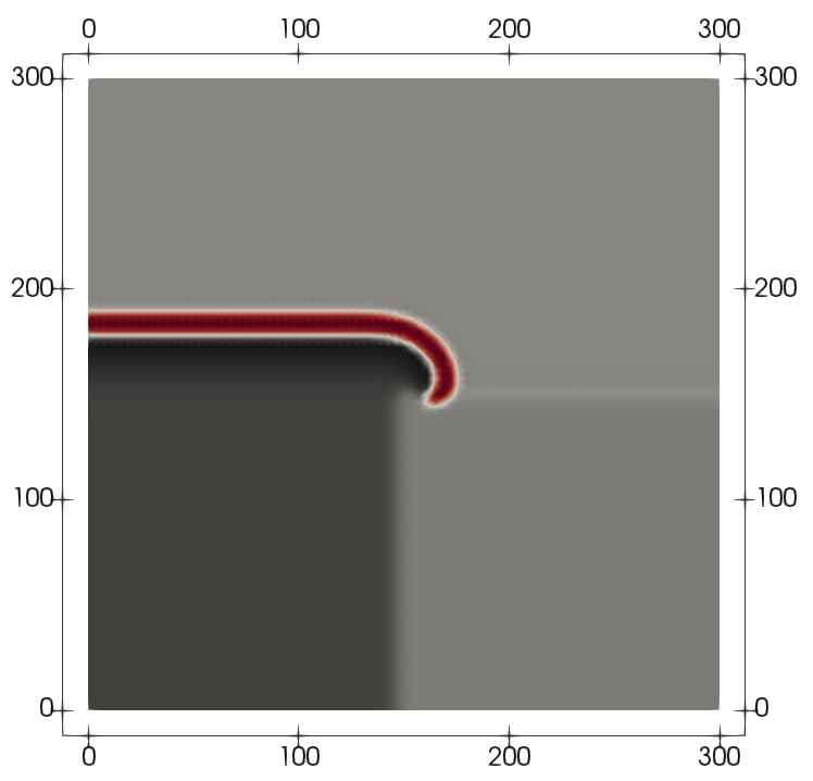
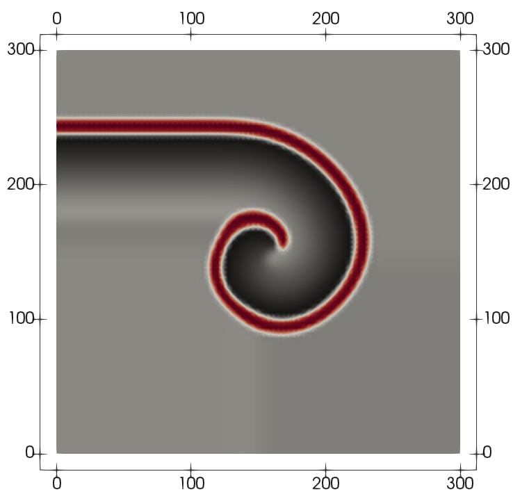
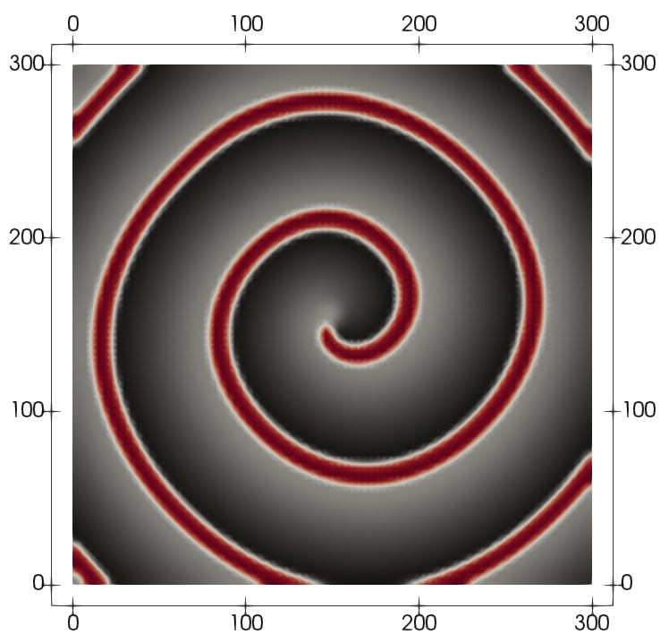
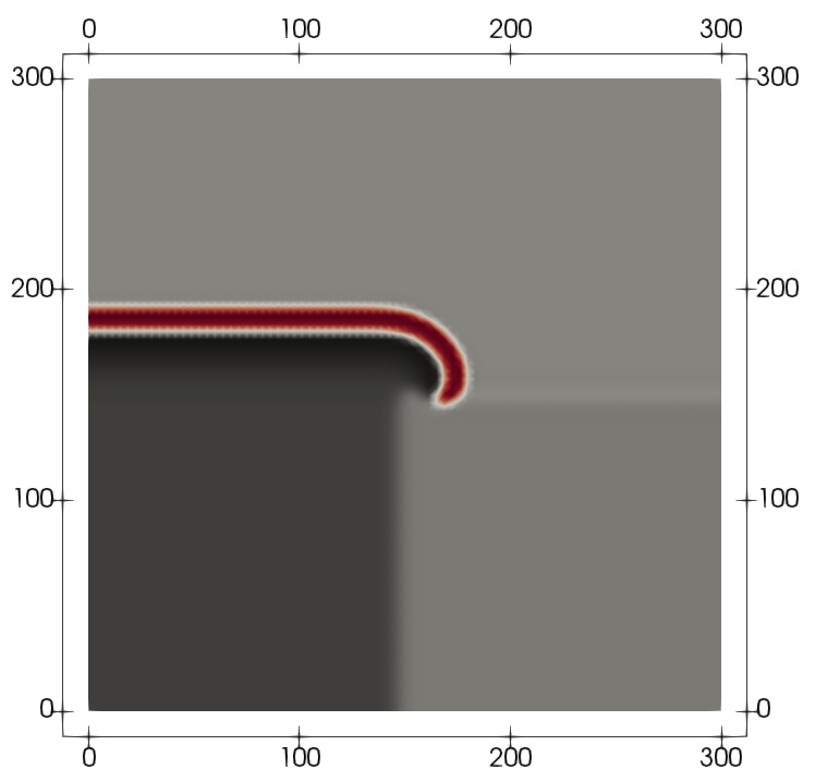
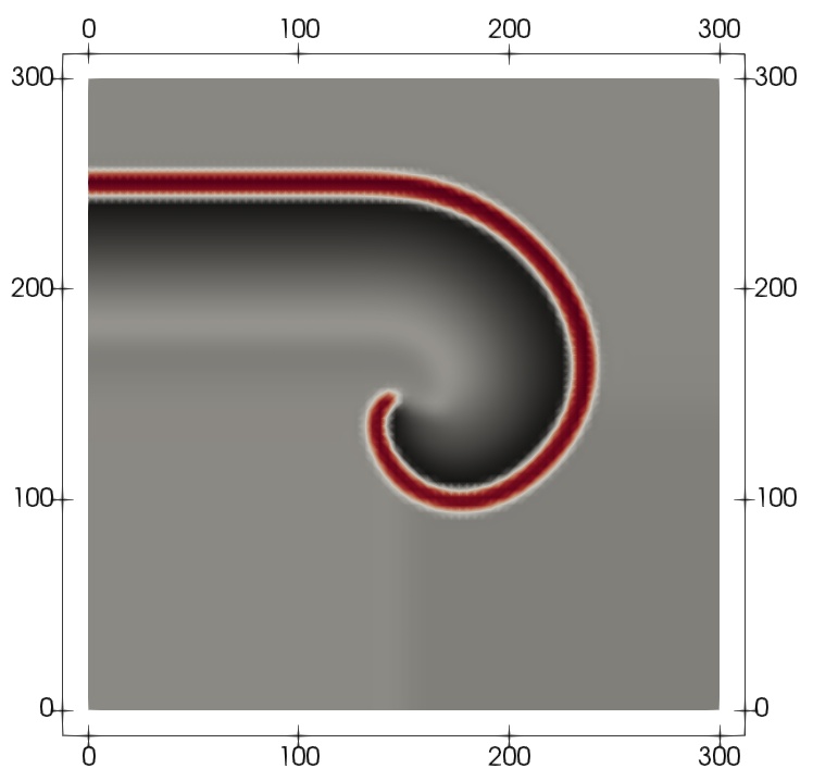
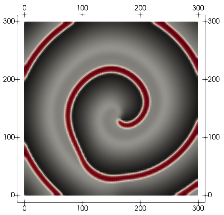
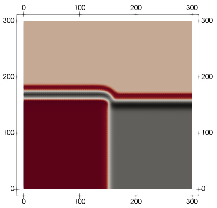
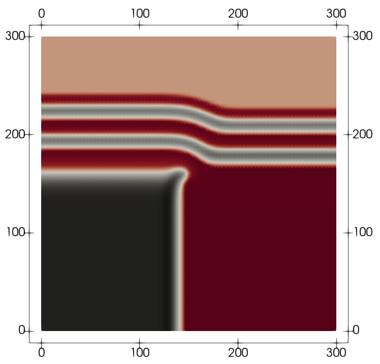
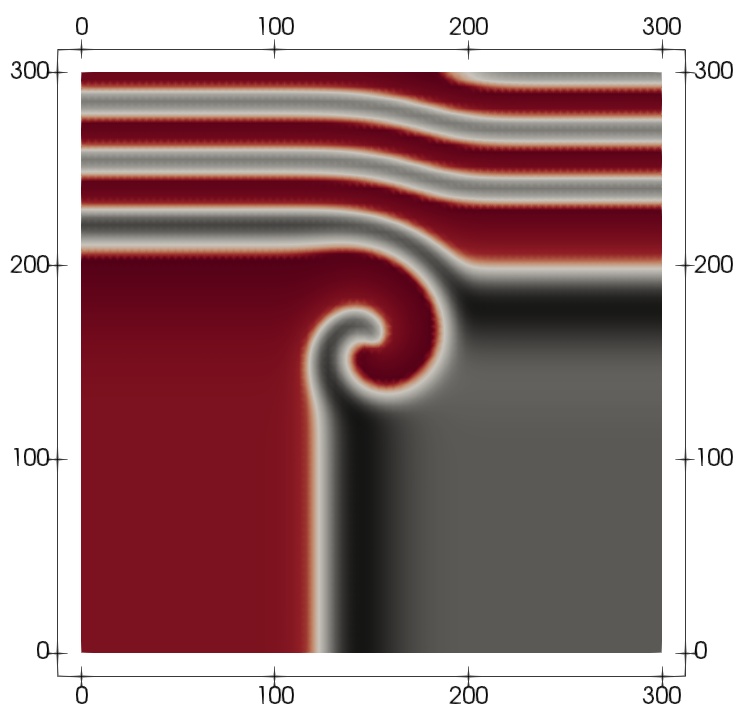
Figure 4.1: Example 3. Snapshots at $t=80,200,650$ of $u_{h}^{DG}$ for the FitzHugh-Nagumo model using $\delta=1$, $\alpha=0$ (top panels) and for the modified generalized Burgers-Huxley system (4.1) with $\delta=1$, $\alpha=0.1$ (middle row) and with $\delta=1.5$, $\alpha=0.1$ (bottom).

5 Conclusion

In this paper we have addressed two main contributions. First, we have proved the well-posedness for the stationary generalized Burgers-Huxley equation. Moreover, we have established a new regularity result that only uses minimal theoretical requirements. Secondly, we have introduced three types of finite element approximations (CFEM, NCFEM and DGFEM) for (1.1). We have rigorously derived a priori error estimates for all of these discretizations. Finally, computational results are given to validate the theoretical first-order convergence of the methods. As a next step we are extending the theory to cover the transient case, and we will also construct efficient and reliable residual-based a posteriori error estimators and adaptive schemes. We also plan to address the formulation of other conservative discretizations using adequate mixed methods.

References

- [1] N. Alinia and M. Zarebnia, A numerical algorithm based on a new kind of tension B-spline function for solving Burgers-Huxley equation, Numerical Algorithms, 82 (2019), pp. 1–22.
- [2] M. S. Alnæs, J. Blechta, J. Hake, A. Johansson, B. Kehlet, A. Logg, C. Richardson, J. Ring, M. E. Rognes, and G. N. Wells, The FEniCS project version 1.5, Archive of Numerical Software, 3 (2015), pp. 9–23.
- [3] D. N. Arnold, An interior penalty finite element method with discontinuous elements, SIAM J. Numer. Anal., 19 (1982), pp. 742–760.
- [4] D. Bini, C. Cherubini, S. Filippi, A. Gizzi, and P. E. Ricci, On spiral waves arising in natural systems, Communications in Computational Physics, 8 (2010), pp. 610–622.
- [5] H. Brezis, Functional Analysis, Sobolev Spaces and Partial Differential Equations, Springer, New York, 1st ed., 2011.
- [6] R. Bürger, R. Ruiz-Baier, and K. Schneider, Adaptive multiresolution methods for the simulation of waves in excitable media, Journal of Scientific Computing, 43 (2010), pp. 261–290.
- [7] I. Çelik, Chebyshev Wavelet collocation method for solving generalized Burgers–Huxley equation, Mathematical Methods in the Applied Sciences, 39 (2016), pp. 366–377.
- [8] Y. Çiçek and G. Tanoglu, Strang splitting method for Burgers–Huxley equation, Applied Mathematics and Computation, 276 (2016), pp. 454–467.
- [9] Z. Chen, A. Gumel, and R. Mickens, Nonstandard discretizations of the generalized Nagumo reaction-diffusion equation, Numerical Methods for Partial Differential Equations, 19 (2003), pp. 363–379.
- [10] P. G. Ciarlet, Linear and Nonlinear Functional Analysis with Applications, SIAM Philadelphia, 1st ed., 2013.
- [11] R. Dautray and J.-L. Lions, Mathematical analysis and numerical methods for science and technology: volume 3 spectral theory and applications, Springer Science & Business Media, 2012.
- [12] V. Ervin, J. Macías-Díaz, and J. Ruiz-Ramírez, A positive and bounded finite element approximation of the generalized Burgers–Huxley equation, Journal of Mathematical Analysis and Applications, 424 (2015), pp. 1143–1160.
- [13] P. Grisvard, Elliptic Problems in Nonsmooth Domains, Pitman, Boston, MA, 1st ed., 1985.
- [14] I. Hashim, M. Noorani, and M. Said Al-Hadidi, Solving the generalized Burgers–Huxley equation using the adomian decomposition method, Mathematical and Computer Modelling, 43 (2006), pp. 1404–1411.
- [15] M. Javidi, A numerical solution of the generalized Burgers-Huxley equation by spectral collocation method, Applied Mathematics and Computation, 178 (2006), pp. 338–344.
- [16] V. John, G. Matthies, F. Schieweck, and L. Tobiska, A streamline-diffusion method for nonconforming finite element approximations applied to convection-diffusion problems, Computer Methods in Applied Mechanics and Engineering, 166 (1998), pp. 85–97.
- [17] A. J. Khattak, A computational meshless method for the generalized Burger’s–Huxley equation, Applied Mathematical Modelling, 33 (2009), pp. 3718–3729.
- [18] B. R. Kumar, V. Sangwan, S. Murthy, and M. Nigam, A numerical study of singularly perturbed generalized Burgers–Huxley equation using three-step Taylor–Galerkin method, Computers & Mathematics with Applications, 62 (2011), pp. 776–786.
- [19] J. E. Macías-Díaz, A modified exponential method that preserves structural properties of the solutions of the Burgers–Huxley equation, International Journal of Computer Mathematics, 95 (2018), pp. 3–19.
- [20] D. K. Maurya, R. Singh, and Y. K. Rajoria, A mathematical model to solve the Burgers-Huxley equation by using new homotopy perturbation method, International Journal of Mathematical Engineering and Management Sciences, 4 (2019), pp. 1483–1495.
- [21] M. T. Mohan and A. Khan, On the generalized Burgers-Huxley equation: Existence, uniqueness, regularity, global attractors and numerical studies, Discrete & Continuous Dynamical Systems-B, 22 (2020), p. 0.
- [22] J. D. Murray, Mathematical Biology, Springer International Publishing, 2002.
- [23] M. Sari, G. Gürarslan, and A. Zeytinoglu, High-order finite difference schemes for numerical solutions of the generalized Burgers–Huxley equation, Numerical Methods for Partial Differential Equations, 27 (2011), pp. 1313–1326.
- [24] J. Satsuma, Exact solutions of Burgers’ equation with reaction terms, Topics in soliton theory and exact solvable nonlinear equations, (1987), pp. 255–262.
- [25] S. Shukla and M. Kumar, Error analysis and numerical solution of Burgers–Huxley equation using 3-scale Haar wavelets, Engineering with Computers, in press (2020).
- [26] R. Temam, Navier-Stokes equations: theory and numerical analysis, vol. 343, American Mathematical Soc., 2001.
- [27] V. Thomée, Galerkin finite element methods for parabolic problems, vol. 1054, Springer, 1984.
- [28] A. K. Verma and S. Kayenat, An efficient Mickens’ type NSFD scheme for the generalized Burgers Huxley equation, Journal of Difference Equations and Applications, 26 (2020), pp. 1213–1246.
- [29] X. Wang, Z. Zhu, and Y. Lu, Solitary wave solutions of the generalised Burgers-Huxley equation, Journal of Physics A: Mathematical and General, 23 (1990), p. 271.
- [30] X.-Y. Wang, Nerve propagation and wall in liquid crystals, Physics Letters A, 112 (1985), pp. 402–406.
- [31] I. Wasim, M. Abbas, and M. Amin, Hybrid B-spline collocation method for solving the generalized Burgers-Fisher and Burgers-Huxley equations, Mathematical Problems in Engineering, 2018 (2018), pp. 1–18.
- [32] O. Y. Yefimova and N. Kudryashov, Exact solutions of the Burgers-Huxley equation, Journal of Applied Mathematics and Mechanics, 3 (2004), pp. 413–420.
- [33] H. Zhou, Z. Sheng, and G. Yuan, Physical-bound-preserving finite volume methods for the Nagumo equation on distorted meshes, Computers & Mathematics with Applications, 77 (2019), pp. 1055–1070.