Anisotropic Field-of-Views in Radial Imaging

Abstract

Radial imaging techniques, such as projection-reconstruction (PR), are used in MRI for dynamic imaging, angiography, and short-$T_{2}$ imaging. They are robust to flow and motion, have diffuse aliasing patterns, and support short readouts and echo times. One drawback is that standard implementations do not support anisotropic field-of-view shapes, which are used to match the imaging parameters to the object or region-of-interest. A set of fast, simple algorithms for 2D and 3D PR, and 3D cones acquisitions are introduced that match the sampling density in frequency space to the desired field-of-view shape. Tailoring the acquisitions allows for reduction of aliasing artifacts in undersampled applications or scan time reductions without introducing aliasing in fully-sampled applications. It also makes possible new radial imaging applications that were previously unsuitable, such as imaging elongated regions or thin slabs. 2D PR longitudinal leg images and thin-slab, single breath-hold 3D PR abdomen images, both with isotropic resolution, demonstrate these new possibilities. No scan volume efficiency is lost by using anisotropic field-of-views. The acquisition trajectories can be computed on a scan by scan basis.

I Introduction

Radial medical imaging methods were first used in X-ray computerized tomography (CT) where data is acquired on radial projections. These projections correspond to radial lines in frequency space, a fact that inspired the first magnetic resonance imaging (MRI) acquisitions to also occur on radial lines[1]. These 2D imaging methods are also known as projection-reconstruction (PR) and projection acquisition (PA). Radial imaging also refers to 3D acquisition techniques such as 3D PR, as well as 3D cones [2, 3].

Radial MRI is used for dynamic imaging applications because it is inherently robust to motion [4] and flow [5]. It is used in angiography[6], with applications such as contrast-enhanced angiography[7, 8] and time-resolved angiography[9]. Radial MRI readouts can support very short repetition times (TRs) and echo times (TEs). Short TRs are useful for steady-state free precession (SSFP) imaging, particularly if high resolution is required or for quadrature fat/water separation. Both the short TRs and robustness to motion and flow have been taken advantage of in balanced SSFP coronary artery imaging [10, 11]. Short TEs are required for ultra-short echo time (UTE) MRI, which can image collagen-rich tissues such as tendons, ligaments and menisci, as well as calcifications, myelin, periosteum and cortical bone [12, 13]. In addition to 2D acquisitions, 3D radial imaging techniques, such as 3D PR [14] and 3D cones [15], have been applied to UTE.

3D PR has also been used for the Vastly undersampled Isotropic Projection Reconstruction (VIPR) imaging method [7] for MR angiography and efficient phase-contrast flow imaging [16]. The isotropic resolution of 3D PR is advantageous for multiplanar and 3D reformats. VIPR uses undersampled acquisitions because the number of projections required for fully-sampled 3D PR is prohibitively large. The undersampling is tolerated because of the diffuse aliasing properties of radial trajectories [7]. Another solution to the often prohibitively large number of projections required by 3D PR is to use conical trajectories [2, 3]. These sample in a spiral pattern along cones with various projection angles, allowing for significantly faster volumetric coverage than 3D PR.

In 2D and 3D PR trajectories, as well as 3D cones, a critical number of projection lines must be acquired to support a given field-of-view (FOV) – also referred to as a region-of-support or region-of-interest. The lines are normally acquired with equiangular spacing, resulting in only circular and spherical FOV shapes. Many imaging applications, however, have anisotropic dimensions and would benefit from anisotropic FOVs.

In this paper we introduce a new method to simply and easily design radial imaging trajectories for anisotropic FOVs. One previous method applied several varying angular density functions to obtain anisotropic 2D FOVs [17, 18]. Our method also utilizes non-uniform angular spacing, and is able to exactly match the sampling to the desired FOV shape. Design algorithms for 2D and 3D PR, as well as 3D cones are presented. Tailoring the FOV for non-circular objects or regions-of-interest allows for scan time reductions without introducing aliasing artifacts. In undersampled applications, this tailoring will reduce the occurrence of aliasing artifacts. Additionally, our algorithms support anisotropic projection lengths, and, equivalently, resolution. This is useful for reducing gradient slew rate demands in 3D cones, and could also be used for reducing gradient distortion artifacts by favoring the more homogeneous or powerful axes. It can also be used to trade image resolution in certain dimensions for acquisition time.

II Theory

In radial imaging, the raw data is acquired on radial lines in frequency space, referred to as “k-space” in MRI. A discrete number of these lines, also known as projections or spokes, are sampled during data acquisition. Sampling theory tells us that the sample separation determines the FOV. Cartesian samples are generally equally spaced, and the FOV is equal to the inverse of the sample spacing, $\frac{1}{\Delta k}$. In radial imaging, the spacing between adjacent projections in k-space varies radially, and is most sparse at the end of the projections. The sample spacing along the projections must also be considered, although in MRI this usually does not limit the FOV as much as the distance between projections. We will investigate how this projection separation determines the FOV and resolution. Further discussion of radial sampling theory can be found in [19].

II-A FOV vs. PSF

The FOV of a given sampling pattern is characterized by its Fourier transform ($\mathcal{FT}$), known as the point spread function (PSF). Since the sampling pattern is multiplied by the frequency data, the PSF is convolved with the image data. The central lobe of the PSF introduces a blurring, and thus determines the resolution of the resulting image. Aliasing lobes in the PSF are outside this central lobe and determine the FOV of the resulting image. In radial imaging, the distinct shape of the aliasing lobe determines the FOV, but they are not always the same shape. Convexity of the aliasing lobe shape in the PSF will ensure that the FOV shape is exactly the same. Polygons, rectangles, cuboids, ellipsoids, and ovals are some examples of convex shapes useful for medical imaging. While there are concave PSF shapes that will support concave FOVs, such as a “plus”-sign shape, we will assume convexity since this includes most objects and regions-of-interest in medical imaging.

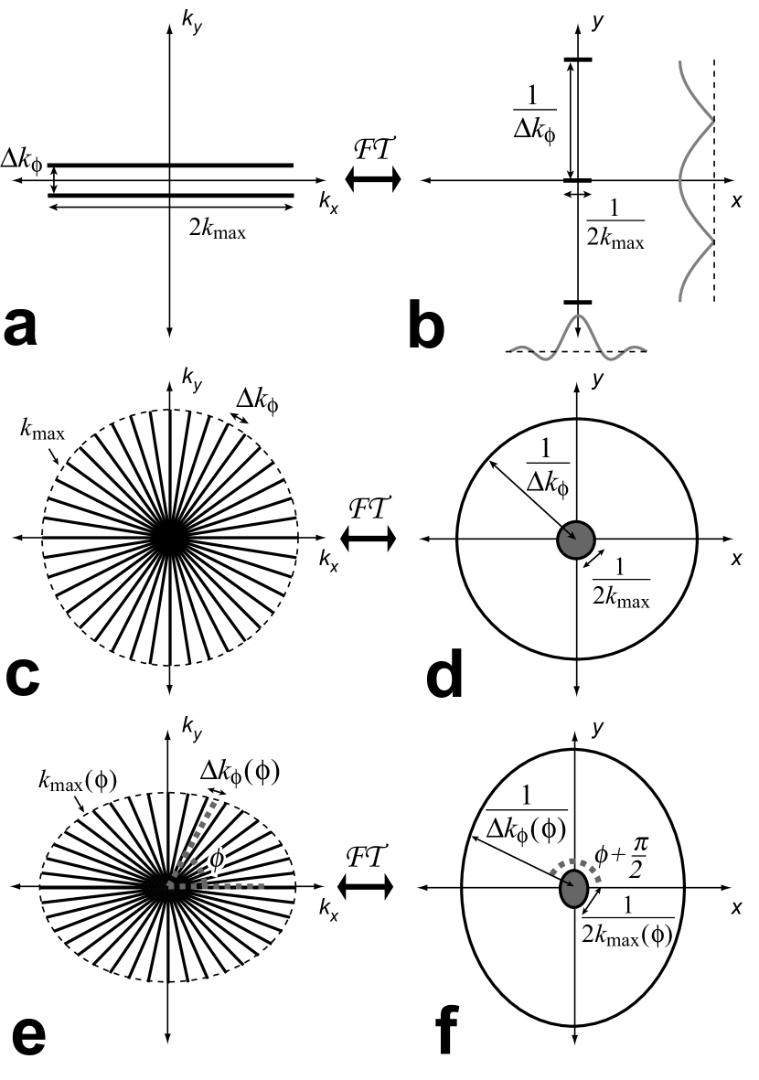
Figure 1: Sampling in 2D radial imaging. (a) Approximation of adjacent projections by parallel sampled lines. (b) Parallel lines PSF illustration. The gray lines show the spatial variation derived in Eq. 2. Aliasing lobes appear at $\frac{1}{\Delta k_{\phi}}$. With additional projections, the aliasing lobes become much sharper that the cosine shown. (c) Isotropic PR trajectory with constant angular spacing and extent. (d) Isotropic PR PSF illustration. (e) PR trajectory with variable angular spacing and extent. (f) Angularly varying PR PSF illustration.

II-B 2D Sampling

The FOV of a 2D radial imaging trajectory can be analyzed by decomposition into adjacent spokes. A pair of adjacent spokes can be approximated as two parallel lines, shown in Fig. 1a and described mathematically as

$$P(k_{x},k_{y})=[\delta(k_{y}-\frac{\Delta k_{\phi}}{2})+\delta(k_{y}+\frac{\Delta k_{\phi}}{2})]\cdot{\rm rect}(\frac{k_{x}}{2k_{\rm max}}),$$ (1)

where $\Delta k_{\phi}$ is the separation at the end of the projections and $k_{\rm max}$ is the length of the projections. The PSF of Eq. 1, illustrated in Fig. 1b, is:

$$\mathcal{FT}\{P(k_{x},k_{y})\}=C\cos(\pi\Delta k_{\phi}y)\cdot{\rm sinc}(2k_{\rm max}x),$$ (2)

where $C$ includes all scaling factors. The peaks of $|\cos(\pi\Delta k_{\phi}y)|$ will introduce aliasing when convolved with the object, thus limiting the FOV perpendicularly to the direction of the lines to $\frac{1}{\Delta k_{\phi}}$. The actual PSF is much more peaked than a cosine because the sample spacings in $k_{y}$ from other projections introduce phase variations that cause the aliasing to cancel out along $y$ between $0$ and $\pm\frac{1}{\Delta k_{\phi}}$, as is shown in the “Results” section. This is analogous to Cartesian sampling where the PSF of two parallel lines is also a cosine but phase variations from the other sampling lines cause sharp aliasing peaks. The resolution is limited to a minimum of $\frac{1}{2k_{\rm max}}$ due the ${\rm sinc}(2k_{\rm max}x)$ term.

If all projections are equally spaced, as shown in Fig. 1c, the alias-free FOV and resolution, $res$, are:

$$FOV = \frac{1}{\Delta k_{\phi}}\approx\frac{1}{k_{\rm max}\Delta\Theta}=\frac{N}{\pi k_{\rm max}},$$ (3)

$$res = \frac{1}{2k_{\rm max}},$$ (4)

where $\Delta\Theta$ is the angular spacing between spokes in radians, $N$ is the number of full projections acquired, and $k_{\rm max}$ is the extent of the spokes in k-space (Fig. 1d). Here we have used the approximation that $\sin(\Delta\Theta)\approx\Delta\Theta$ for small $\Delta\Theta$.

From Fourier theory, rotation of the parallel lines rotates their $\mathcal{FT}$, thus the angular spacing between spokes can be varied to produce anisotropic FOV shapes. Similarly, if $k_{\rm max}$ is varied, the resolution size changes angularly. Equation 2 tells us that the sample spacing at angle $\phi$ determines the perpendicular FOV, while $k_{\rm max}$ at $\phi$ determines the resolution at $\phi$. This is shown in Fig. 1e and f, and is formally expressed as,

$$FOV(\phi+\frac{\pi}{2}) = \frac{1}{\Delta k_{\phi}(\phi)}\approx\frac{1}{k_{\rm max}(\phi)\Delta\Theta(\phi)},$$ (5)

$$res(\phi) = \frac{1}{2k_{\rm max}(\phi)}.$$ (6)

Discrete sampling along the parallel lines results in repetition of the $\mathcal{FT}$ pattern (Eq. 2) in this sampling direction ($x$ in Eq. 2 and Fig. 1a). Radial sample spacing of $\Delta k_{r}$ results in repetitions at $\frac{1}{\Delta k_{r}}$. These aliasing lobes are often eliminated in MRI because of low-pass filters applied during the readout. These filters will, however, limit the FOV in the projection direction to $\frac{1}{\Delta k_{r}}$ because they are matched to the sample spacing. Therefore, the maximum radial sampling spacing must be

$$\Delta k_{r}\leq\frac{1}{\max(FOV(\phi))}$$ (7)

to ensure there is no aliasing or FOV restrictions due to the sampling along the projections.

II-C 3D Sampling

Radial sampling in 3D can be analyzed with the same principles as in 2D. Again, approximating adjacent spokes as a set of parallel lines, we now have:

$$P(k_{x},k_{y},k_{z}) = [\delta(k_{y}-\frac{\Delta k_{\phi}}{2})+\delta(k_{y}+\frac{\Delta k_{\phi}}{2})]\cdot$$ (8)

$${\rm rect}(\frac{k_{x}}{2k_{\rm max}})\cdot\delta(k_{z}).$$

The PSF is then the same as Eq. 2:

$$\mathcal{FT}\{P(k_{x},k_{y},k_{z})\}=K\cos(\pi\Delta k_{\phi}y)\cdot{\rm sinc}(2k_{\rm max}x).$$ (9)

This aliasing pattern is the same as illustrated in Fig. 1b, but with an infinite extent in $z$.

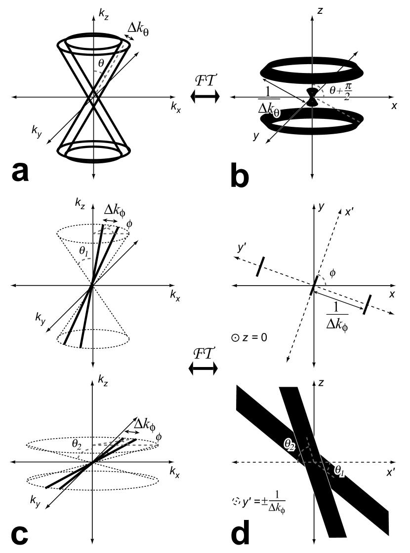
Figure 2: Sampling in 3D radial imaging. (a) Approximation of adjacent cones by rotated parallel lines. (b) PSF illustration of adjacent cones model, which is the parallel lines PSF (Fig. 1b) rotated around the $z$-axis. (c) Adjacent projections on two different cones. (d) PSF illustrations for the adjacent projections. The top illustration shows the intersection of the PSF with the $x$-$y$ plane, which is approximately identical for the projections on both cones. The bottom illustration shows the planes which contain the aliasing lobes. These planes are perpendicular to the $y^{\prime}$ axis at $y^{\prime}=\pm 1/\Delta k_{\phi}$, and the lobes extend and different angles depending on the cone angle.

A set of adjacent cones can be modeled by rotating a pair of parallel lines about the $k_{z}$-axis, as shown in Fig. 2a, which rotates the PSF of these parallel lines about the $z$-axis. The resulting PSF pattern is circularly symmetric about the $z$-axis and with polar deflection of the aliasing lobe of $\theta+\frac{\pi}{2}$ for a cone deflection of $\theta$, shown in Fig. 2b. We are using the spherical coordinate notation where $\theta$, the polar angle, is the deflection from the positive $z$-axis and $\phi$, the azimuthal angle, is the rotation from the positive $x$-axis.

Adjacent projections on a cone produce aliasing patterns that are rotations of the PSF in Eq. 9, as illustrated in Fig. 2c and d. The aliasing lobes are the nearest to the origin in the $x$-$y$ plane at an azimuthal angle $\phi+\frac{\pi}{2}$ and at a distance of $1/\Delta k_{\phi}$.They extend in a direction that is determined by the cone deflection angle, as shown in Fig. 2d.

Combining these results, we find that the sampling along a cone limits the FOV azimuthally in the $x$-$y$ plane while the sampling of different cones limits the FOV in the polar direction. Mathematically,

$$FOV_{\theta}(\theta+\frac{\pi}{2},\phi) = \frac{1}{\Delta k_{\theta}(\theta)}$$ (10)

$$FOV_{\phi}(\theta=\frac{\pi}{2},\phi+\frac{\pi}{2}) = \frac{1}{\Delta k_{\phi}(\phi)}$$ (11)

$$res(\theta,\phi) = \frac{1}{2k_{\rm max}(\theta,\phi)},$$ (12)

where the variables are all illustrated in Fig. 2. The resolution is determined by the projection extents. The samples along the projection must again satisfy Eq. 7.

III Methods

III-A 2D Projection-Reconstruction

Two-dimensional radial imaging trajectories can be defined by the projection angles, projection lengths, and the sampling pattern along the projections. Our algorithm designs a set of projection angles, $\Theta[n]$, and projection lengths, $K_{\rm max}[n]$, for a desired FOV pattern. The sampling pattern along the projections is not designed, and should be chosen to meet the condition in Eq. 7.

1. Initialize $\Theta[1]=\phi_{0}$ and $n=1$ 2. Calculate: $$\displaystyle\Delta\Theta_{\rm est}=\frac{\textstyle 1}{\textstyle k_{\rm max}(\Theta[n])FOV(\Theta[n]+\frac{\pi}{2})}$$ $$\displaystyle\Delta\Theta=\frac{\textstyle 1}{\textstyle k_{\rm max}(\Theta[n]+\frac{\Delta\Theta_{\rm est}}{2})FOV(\Theta[n]+\frac{\Delta\Theta_{\rm est}}{2}+\frac{\pi}{2})}$$ $$\displaystyle\Theta[n+1]=\Theta[n]+\Delta\Theta$$ and increment $n$ 3. Repeat previous step until $\Theta[n]>\phi_{0}+\phi_{\rm width}$ 4. Choose a scaling factor, $S$, and the number of projections returned, $N$, as follows:
If $\Theta[n]-(\phi_{0}+\phi_{\rm width})<(\phi_{0}+\phi_{\rm width})-\Theta[n-1]$
     choose $S=\frac{\textstyle\phi_{\rm width}}{\textstyle\Theta[n]-\phi_{0}}$ and $N=n-1$
Else
     $S=\frac{\textstyle\phi_{\rm width}}{\textstyle\Theta[n-1]-\phi_{0}}$ and $N=n-2$
5. Scale the set of angles
$\Theta[1,\ldots,N]=S\cdot(\Theta[1,\ldots,N]-\phi_{0})+\phi_{0}$ 6. Calculate $K_{\rm max}[n]=k_{\rm max}(\Theta[n])$

Figure 3: Generalized 2D anisotropic FOV radial imaging algorithm

The algorithm is shown in Fig. 3. The desired FOV must be specified as a function of angle, $FOV(\phi)$, and must be $\pi$-periodic ($FOV(\phi)=FOV(\phi+\pi)$). The desired projection lengths can be specified as $k_{\rm max}(\phi)$, and also must be $\pi$-periodic. An initial angle of $\phi_{0}$ may be specified, although the default of $\phi_{0}=0$ is appropriate for most applications. The angular width of the resulting angles, $\phi_{\rm width}$, may also be specified, and will be $\pi$ for most applications, including full-projection PR. One application of varying this width is half-projection PR, where $\phi_{\rm width}=2\pi$ could be used. These parameters are also useful for designing 3D PR trajectories - see Section III-C.

After initialization, the relationship derived in Eq. 5 is used to sequentially calculate a set of projection angles in step 2 of the algorithm. The projection separation is first estimated, $\Delta\Theta_{\rm est}$, and then the actual projection separation is then calculated using the angle $\Theta[n]+\frac{\Delta\Theta_{\rm est}}{2}$. Without this estimation, the resulting FOV will be very slightly rotated and distorted because the projection separation is centered between $\Theta[n]$ and $\Theta[n+1]$. Since $\Theta[n+1]$ is unknown, $\Theta[n]+\frac{\Delta\Theta_{\rm est}}{2}$ provides a good estimate of the middle angle, especially compared to using $\Theta[n]$. Additional iterations for increased accuracy are possible but provide little additional benefit.

The sequential nature of the algorithm and the required periodicity of the projection angles results in an undesired angle spacing at the end of the design. Steps 4 and 5 correct for this by scaling the set of projection angles to the chosen $\phi_{\rm width}$. The scaling slightly distorts the resulting FOV shape so the scaling factor, $S$, is chosen by step 4 to be as close to 1 as possible.This step could also be modified to require that the number of projections be even, odd, or a scalar multiple for acquisition strategies such as multi-echo PR [8].

The computation cost of this algorithm is small since it involves simple calculations and requires no iterations or large matrix operations.

III-B 3D Cones

The 2D design algorithm can directly be applied to designing 3D cones imaging trajectories. The 3D FOV shapes that are achievable are circularly symmetric about one axis, which we define to be the $z$-axis, corresponding to cones wrapping around the $k_{z}$-axis as shown in Fig. 2a and b. These shapes can be described by $FOV(\theta,\phi)=FOV_{\theta}(\theta)$, as is illustrated in Fig. 4a and b. For example, a rectangular-shaped $FOV_{\theta}(\theta)$ will yield a cylindrical FOV, while an elliptical $FOV(\theta)$ yields an ellipsoid.

For anisotropic 3D cones design, the 2D PR algorithm is used with inputs of $FOV(\theta)$ and $k_{\rm max}(\theta)$ (optional), $\phi_{\rm width}=\pi$, and $\phi_{0}=\frac{1}{2k_{\rm max}(0)FOV(\frac{\pi}{2})}$. This $\phi_{0}$ ensures that no cones are just a single projection. The resulting set of projection angles and extents describe the set of cones to be used, where the angles, $\Theta[n]$, represent the deflection from the $k_{z}$-axis. Sampling within each cone and generation of appropriate gradient waveforms are described in [3].

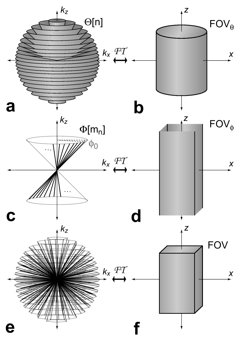
Figure 4: 3D radial trajectory design (cones-based). (a) Cones designed with 2D algorithm. (b) Sampling of cones introduces $FOV_{\theta}$, which is circularly symmetric about the $z$-axis. (c) Projections on each cone designed with 2D algorithm using a random starting angle $\phi_{0}$. (d) Sampling along cones introduces $FOV_{\phi}$, which is approximately independent of $z$. (e) 3D PR trajectory resulting from sampling in (a) and (c). (f) The 3D PR FOV is the minimum of $FOV_{\theta}$ (b) and $FOV_{\phi}$ (d).

III-C 3D Projection-Reconstruction

We have created two methods for designing 3D PR trajectories with anisotropic FOVs. One samples a set of cones, the “cones-based” method, while the other designs and samples a spiraling path, the “spiral-based” method. Figure 5 shows two resulting sampling patterns for both the cones-based and spiral-based design methods.

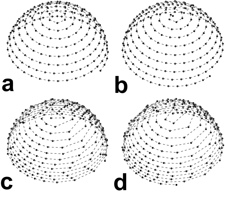
Figure 5: 3D PR trajectories. (a) Cones-based design, and (b) Spiral-based design for uniform sampling, resulting in a spherical FOV. (c) Cones-based design, and (d) Spiral-based design of an ellipsoid FOV with, non-uniform sampling in both the azimuthal and polar directions.

III-C1 Cones-based Design

This method designs 3D projections for an anisotropic FOV by first designing a set of cones and then appropriately sampling on each cone. Isotropic sampling in these two dimensions will result in a spherical FOV, with the number of projections per cone proportional to $\sin(\theta)$ [20], where $\theta$ is the polar angle of the cone.

Equations 10 and 11, illustrated in Fig. 2, tell us that the cones sampled will define a limiting FOV that is circularly symmetric about the $z$-axis, $FOV_{\theta}(\theta,\phi)=FOV_{\theta}(\theta)$, while the samples on each cone define a maximum FOV that is approximately invariant in $z$, $FOV_{\phi}(\theta,\phi)\approx FOV_{\phi}(x,y)$ (Fig. 4a-d). We will describe $FOV_{\phi}$ using the deflection angle in cylindrical coordinates, $\phi_{c}$, resulting in the simple notation $FOV_{\phi}(x,y)=FOV_{\phi}(\phi_{c})$. Both sampling patterns limit the FOV, resulting in

$$FOV=\min(FOV_{\theta}(\theta),FOV_{\phi}(\phi_{c})),$$ (13)

as illustrated in Fig. 4e and f.

This method takes inputs of $FOV_{\theta}$ and $FOV_{\phi}$, with

$$FOV_{\phi}(\phi_{c})\leq FOV_{\theta}(\frac{\pi}{2})$$ (14)

to ensure that the cone spacing does not introduce aliasing inside $FOV_{\phi}$ in the $x$-$y$ plane. $k_{{\rm max},\theta}(\theta)$ can also be used. Varying $k_{{\rm max},\phi}$ has not been incorporated into our algorithm because it causes the polar angle spacing to vary azimuthally, resulting in distortion of the supported FOV. The cones are designed using the 2D PR algorithm with $FOV_{\theta}(\theta)$, $k_{{\rm max},\theta}(\theta)$, $\theta_{0}=0$, and $\theta_{\rm width}=\frac{\pi}{2}$. The resulting $\Theta[n]$ and $K_{\rm max}[n]$, where $n=1,\ldots,N_{cones}$, are then sampled, also using the 2D PR design algorithm.

The spokes covering each cone are designed with $FOV_{\phi}(\phi_{c})$ and $\phi_{\rm width}=2\pi$. For cone $n$, $k_{{\rm max},\phi}=K_{\rm max}[n]\cdot\sin(\Theta[n])$ to adjust for the circumference of the cone. The initial angle $\phi_{0}$ on each cone is chosen at random uniformly in the interval $[0,\frac{1}{K_{\rm max}[n]\cdot\sin(\Theta[n])\cdot FOV_{\phi}(\frac{\pi}{2})}]$. This randomization reduces coherent aliasing artifacts that are introduced when $\phi_{0}=0$ for each cone (see Fig. 10). Note that the first cone ($n=1$) is just a single projection along the $k_{z}$-axis. The result is a set of $\Phi[m_{n}]$ for $m_{n}=1,\ldots,M_{n}$ and $n=1,\ldots,N_{cones}$, where $M_{n}$ is the number of projections within cone $n$.

To complete the full-projection design, an additional cone is added in the $k_{x}$-$k_{y}$ plane ($\theta=\frac{\pi}{2}$) that is only azimuthally sampled along half of the circumference. The 2D PR design algorithm is used, with $FOV_{\phi}(\phi_{c})$, $k_{{\rm max},\phi}=k_{{\rm max},\theta}(\frac{\pi}{2})$, a randomized $\phi_{0}$, and $\phi_{\rm width}=\pi$. For half-projection designs, the additional half-sampled cone is not needed and $\theta_{\rm width}=\pi$ is used for the cone design.

III-C2 Spiral-based Design

This method of 3D PR design is inspired by a method that isotropically samples the unit sphere on a spiral path [21]. The design is similar to the cones-based method, taking the same inputs of $FOV_{\theta}$ and $FOV_{\phi}$, with $FOV_{\theta}(\frac{\pi}{2})={\rm max}(FOV_{\phi}(\phi_{c}))$, and, optionally, $k_{{\rm max},\theta}$. This method is best suited for half-projections, and an extension to full-projection design is described in Appendix A. It also results in a more diffuse aliasing pattern (see Fig. 10).

First, a set of polar sampling angles is designed with the 2D PR algorithm exactly as in the cones-based method for half-projections, with $FOV_{\theta}$, $k_{{\rm max},\theta}$, $\theta_{0}=0$, and $\theta_{\rm width}=\pi$, yielding $\hat{\Theta}[n]$ and $\hat{K}_{\rm max}[n]$ for $n=1,\ldots,N_{polar}$. To create a continuous sample sample path in the longitudinal direction, these sets are linearly interpolated to final samples of $\hat{\Theta}[N_{polar}+1]=\pi$ and $\hat{K}_{\rm max}[N_{polar}+1]=k_{{\rm max},\theta}(\pi)$.

The interpolation uses the number of projections required, which is found by estimation using the required number of azimuthal samples on a cone at $\theta=\frac{\pi}{2}$, $N_{\phi,{\rm est}}$, as well as $\hat{\Theta}[n]$ and $\hat{K}_{\rm max}[n]$. The 2D PR algorithm with $FOV_{\phi}$, $k_{{\rm max},\phi}=k_{{\rm max},\theta}(\frac{\pi}{2})$, $\phi_{0}=0$, and $\phi_{\rm width}=2\pi$ is used to compute $N_{\phi,{\rm est}}$. The number of projections between $\hat{\Theta}[n]$ and $\hat{\Theta}[n+1]$ will be approximately

$$N_{n,{\rm est}} = N_{\phi,{\rm est}}\sin(\frac{\hat{\Theta}[n]+\hat{\Theta}[n+1]}{2})$$ (15)

$$\times\frac{\hat{K}_{\rm max}[n]+\hat{K}_{\rm max}[n+1]}{2k_{{\rm max},\phi}}.$$

The total number of projections is chosen to be

$$N=\sum_{n=1}^{N_{polar}}N_{n,{\rm est}}.$$ (16)

The linear interpolation is done such that there are $N_{n,{\rm est}}$ projections between $\hat{\Theta}[n]$ and $\hat{\Theta}[n+1]$. This is done by using a parametrization, $\theta(t)$, where $\theta(t_{n})=\hat{\Theta}[n]$, $t_{n+1}-t_{n}=N_{n,{\rm est}}$, and $t_{1}=1$. The polar projection angles are computed by sampling the linear interpolation of this parametrization as $\Theta[m]=\theta(m)$ for $m=1,\ldots,N$. If variable extents are used, the interpolation of $k(t)$, where $k(t_{n})=\hat{K}_{\rm max}[n]$, is sampled as $K_{\rm max}[m]=k(m)$.

The azimuthal sampling, $\Phi[m]$, is then computed similarly to step 2 in Fig. 3, with an additional scaling factor also used in the cones-based design to compensate the cone circumference:

$$\Delta\Phi_{\rm est}=\frac{1}{K_{\rm max}[m]\sin(\Theta[m])FOV_{\phi}(\Phi[m]+\frac{\pi}{2})}$$ (17)

$$\Delta\Phi=\frac{1}{K_{\rm max}[m]\sin(\Theta[m])FOV_{\phi}(\Phi[m]+\frac{\Delta\Phi_{\rm est}}{2}+\frac{\pi}{2})}$$ (18)

$$\Phi[m+1]=\Phi[m]+\Delta\Phi,$$ (19)

with the initial angle of $\Phi[1]=0$. This results in a set of projection angles, $\Phi[m]$, $\Theta[m]$, and extents, $K_{\rm max}[m]$ yielding the anisotropic FOV described in Eq. 13.

III-D Reconstruction

All images were reconstructed with the gridding algorithm [22], and PSFs were calculated by gridding data of all ones. Each data point is multiplied by a density compensation factor (dcf) to correct for the unequal sample spacing, which results in coloring of the noise and an intrinsic loss in the signal-to-noise ratio (SNR) efficiency [23]. The dcf can be separated into a radial and angular components, where the angular component accounts for the anisotropic projection spacing. The angular dcf is chosen so that the same radial dcf can be used on each projection, provided they all have an equal number of identically distributed radial samples. When the samples are equally spaced this radial component is linear for 2D PR and quadratic for 3D PR.

The 2D angular dcf ($D_{\theta}$) is proportional to the projection separation, $\Delta k_{\phi}$, given from Eq. 5. For a separable dcf, $D_{\theta}$ must also be proportional to the projection length because the scaling of the radial sample spacing by $k_{\rm max}$ cannot be described in a single radial dcf. The resulting 2D PR angular dcf is

$$D_{\theta}(\Theta[n])=K_{\rm max}[n]\cdot\Delta k_{\phi}=\frac{K_{\rm max}[n]}{FOV(\Theta[n]+\frac{\pi}{2})}.$$ (20)

For anisotropic 3D cones, this compensation factor is applied to each cone by dividing Eq. 10 in reference [3] by $D_{\theta}$. In 3D PR, the density compensation for a given projection is found by multiplying the compensation factors for the polar and azimuthal sampling:

$$D_{3D}(\Theta[n],\Phi[m_{n}])=D_{\theta}(\Theta[n])\times D_{\phi}(\Phi[m_{n}])\\ =\frac{K_{\rm max}[n]}{FOV_{\theta}(\Theta[n]+\frac{\pi}{2})\times FOV_{\phi}(\Phi[m_{n}]+\frac{\pi}{2})}.$$ (21)

For the full-projection spiral-based design, this dcf is slightly modified as described in Appendix A.

III-E Design Functions

The anisotropic FOVs were designed in Matlab 7.0 (The Mathworks, Natick, MA, USA). The design functions for 2D PR, 3D cones, and both 3D PR methods, along with accompanying documentation are available for general use at http://www-mrsrl.stanford.edu/~peder/radial_fovs.

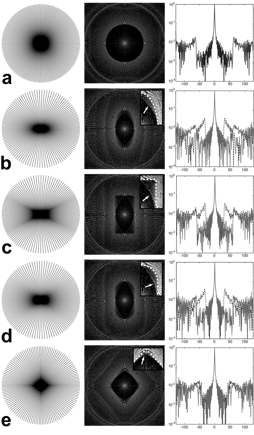
Figure 6: Projection sampling patterns (left column) and PSFs (middle column), with plots along $x$ (black, dashed line) and $y$ (gray line) axes in the right column. FOV shapes: (a) Circle, (b) Ellipse, (c) Rectangle, (d) Oval, and (e) Diamond. The inset PSF images are windowed narrowly to show the low-level aliasing (arrows) within the desired FOV (dashed lines). The plots show the aliasing peaks and the isotropic resolution in the central lobes. Small FOVs are used for visualization of the variable angular density.

III-F MRI Experiments

A GE Excite 1.5T scanner with gradients capable of 40 mT/m amplitude and 150 T/m/s slew rate (GE Healthcare, Milwaukee, WI) was used for all experiments. The 2D PR images were acquired with a UTE sequence using half-projection acquisitions, 5 mm slice thickness, TE = 500 $\mu$s, TR = 100 ms, 30^∘ flip angle, 512 samples per projection, and 1 mm resolution with a transmit/receive extremity coil. The 3D PR images were acquired with a spoiled gradient-recalled echo (SPGR) sequence using full-projection acquisitions with TE = 3 ms and TR = 10 ms. The bottle phantom images used a 15^∘ flip angle, 256 samples per projection, and 1 mm isotropic resolution with a transmit/receive head coil. The in vivo images used a 30^∘ flip angle, 3 cm slab-selective RF excitation, 192 samples per projection, a body coil, and were acquired in a single 25 second breath-hold. Both fully-sampled and undersampled cylindrical FOVs with 3 and 2 mm isotropic resolution, respectively, are compared to isotropic FOVs requiring the same number of projections.

IV Results

IV-A 2D PSFs

Figure 6 shows some sampling patterns designed with the 2D anisotropic FOV algorithm and their corresponding PSFs, showing that the desired FOV shapes are achieved. They have isotropic resolution, as shown in the PSF central lobes. There is some low-level aliasing introduced inside the desired FOV for the anisotropic shapes, shown in the inset PSF images. See Section V for a full discussion.

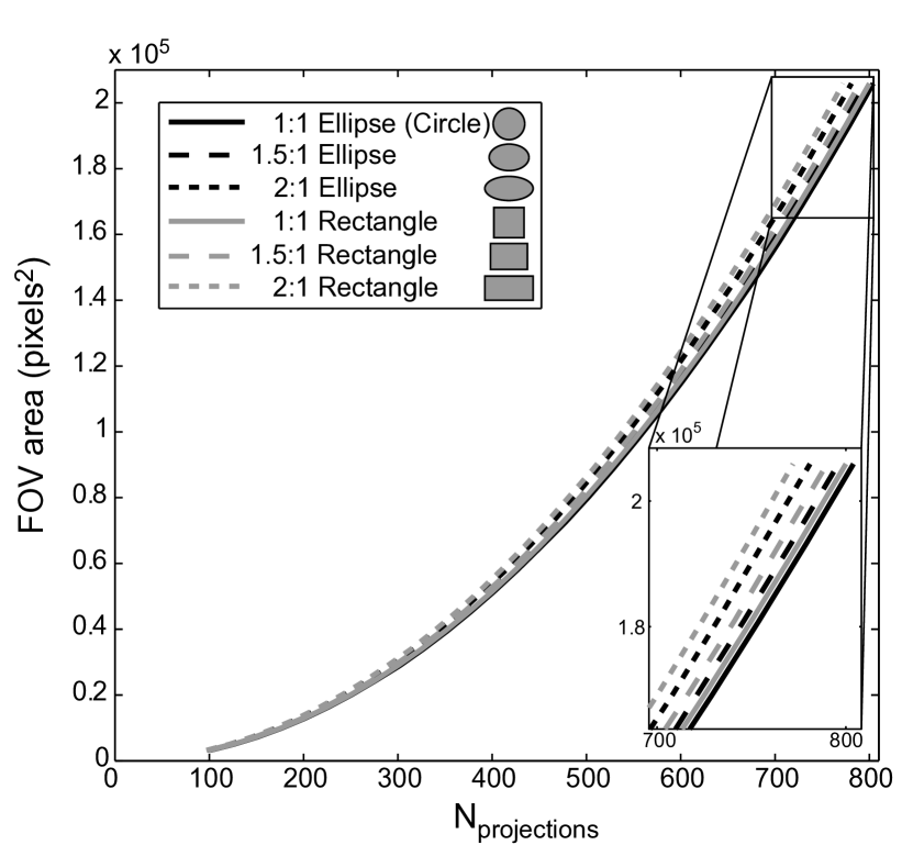
Figure 7: Number of projections for elliptical and rectangular FOV shapes versus the resulting FOV (shape) area. All the FOVs have 1 pixel isotropic resolution. There is no loss in efficiency by using anisotropic shapes, and in fact they are slightly more efficient than the isotropic case. This increase in efficiency comes at the cost of low-level aliasing within the FOV, seen in Fig. 6.

Figure 7 shows the relationship between the number of projections and the FOV area for elliptical and rectangular FOV shapes. The relationship is quadratic for a circular FOV, and the other shapes are also approximately quadratic. The anisotropic shapes are slightly more efficient, with efficiency increasing as the shapes become narrower. This is due to the low-level aliasing seen in Fig. 6, which is larger for narrower shapes (see Section V).

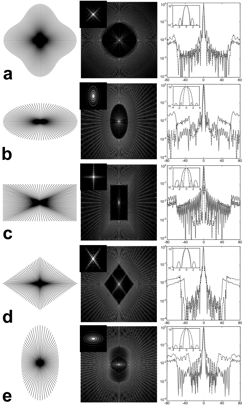
Figure 8: Variable $k_{\rm max}$ sampling patterns (left column) and PSFs (middle column, plots in right column), with enlarged views of the central lobe inset. The black, dashed line plot is along the $x$-axis, and the gray line is along the $y$-axis in (b), (c), and (e), and along $x=y$ in (a) and (d). FOV/$k_{\rm max}$ shapes: (a) Circle/Star, (b) Ellipse/Ellipse, (c) Rectangle/Rectangle, (d) Diamond/Diamond, and (e) Oval/Ellipse. All the combinations have a minimum resolution size of 1 pixel, with maximum resolutions 2 pixels in (a), (b), and (e), 1.72 pixels in (c), and 1.33 pixels in (d). The shape combinations in (b), (c), and (d) have no low-level aliasing inside the FOV shape, unlike (a) and (e), and the isotropic resolution projections in Fig. 6. Small FOVs are used for visibility of the variable angular density.

Some sampling patterns with variable $k_{\rm max}$ patterns and their corresponding PSFs are shown in Figure 8. The angularly varying projection lengths results in anisotropic resolution, seen in the main lobe of the PSFs. There is again some low-level aliasing introduced inside the desired FOV in Fig. 8a and e, but there is none of this aliasing in b, c, and d. For these three sampling patterns, $k_{\rm max}$ is the dual of the FOV shape, or $k_{\rm max}(\phi)\propto FOV(\phi+\frac{\pi}{2})$. In this case, the width of the aliasing lobes is inversely proportional to the FOV and the angular density compensation, $D_{\theta}$, is uniform (Eq. 20). See Section V for more discussion of the dual shapes. Reducing the resolution also reduces the number of projections required. For the same FOV shapes with isotropic resolution, the trajectories in Fig. 8 require between 13 and 36% less projections, demonstrating the trade-off that can be made between resolution in a given dimension and acquisition time.

Animations of how the PSF evolves as the algorithm progresses are available at http://www-mrsrl.stanford.edu/~peder/radial_fovs. The principles of the sampling approximations used (Fig. 1) are visible in the movies.

IV-B 3D PSFs

The PSFs for 3D cones trajectories are 2D PR PSFs rotated about one axis, as is illustrated in Fig. 4a and b.

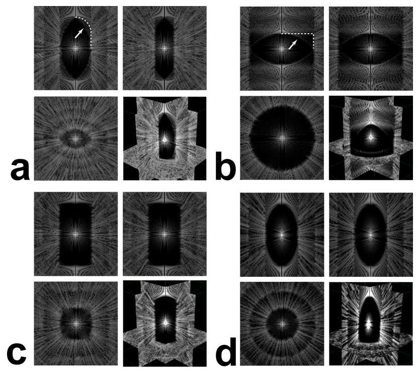
Figure 9: PSFs for 3D PR trajectories with anisotropic FOVs using the spiral-based design. FOVs: (a) Oval $FOV_{\theta}$ and ellipse $FOV_{\phi}$, (b) Cylinder, (c) Cuboid, and (d) Ellipsoid with an ellipsoid $k_{{\rm max},\theta}$ shape, shrunk in the $k_{z}$ direction. The top row for each shape shows the PSF in the $y=0$ and $x=0$ planes, and the bottom row shows the $z=0$ plane and a 3-plane view. Similarly to the 2D case, there is some low-level aliasing (arrows) inside the desired FOV shapes (dashed lines), which is particularly visible in (b).

Figure 9 shows some PSFs for spiral-based 3D PR sampling patterns. For the variety of shapes and dimensions, the desired FOV is achieved, and using an oval for $FOV_{\theta}$ and ellipse for $FOV_{\phi}$ (Fig. 9a) results in three different FOV dimensions. There are low-level aliasing artifacts present in these PSFs (arrows in Fig. 9a and b). The cuboid (Fig. 9c) has sharp corners in all three dimensions, and is also well-defined at non-zero $z$-values, demonstrating that the azimuthal sampling aliasing shape, $FOV_{\phi}$, is invariant in $z$, as assumed in Eq. 13. The PSF of an ellipsoid FOV with an ellipsoid $k_{{\rm max},\theta}$ is shown in Fig. 9d, demonstrating that variable $k_{{\rm max},\theta}$ is feasible. This trajectory has a 50% reduction in Z-gradient strength requirements compared to the other trajectories because $k_{{\rm max},\theta}$ limits the projection extents in $k_{z}$. This halves the resolution in $z$, but requires 33% less projections than the same FOV shape with 1 pixel isotropic resolution.

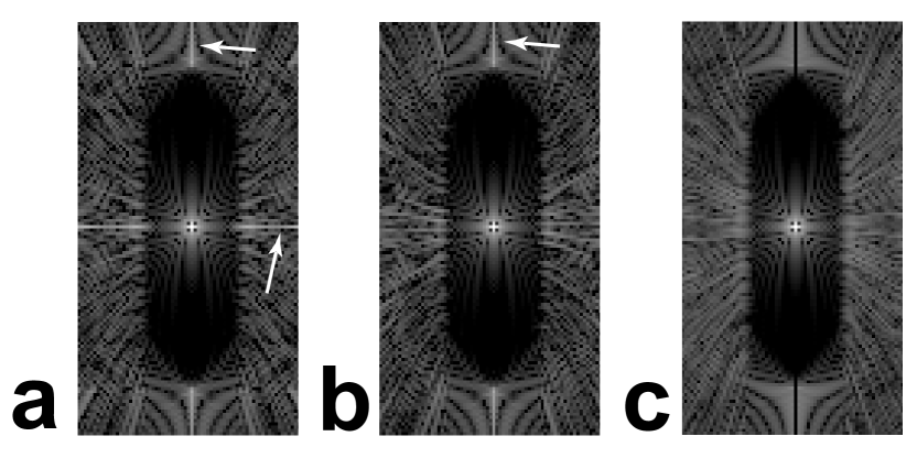
Figure 10: PSFs for various 3D PR design methods. (a) Cones-based design without randomized $\phi_{0}$. (b) Cones-based design with randomized $\phi_{0}$. (c) Spiral-based design. The $x=0$ plane for the shape in Fig. 9a is shown, and the images are identically windowed. The arrows indicate coherent streaking artifacts, all of which are eliminated when using the spiral-based design.

Coherent aliasing lines are introduced when using the cones-based design, as shown in Fig. 10. The use of a random $\phi_{0}$ in the cones-based design eliminates the coherent line in the $x$-$y$ plane. A line along the $z$-axis remains because the polar projection spacings around $\theta=\frac{\pi}{2}$ are all identical. The tilt of the spiral in $k_{z}$ diffuses the line in the spiral-based design. These coherent lines would not affect fully-sampled acquisitions. In undersampled applications, which take advantage of the diffuse 3D PR aliasing, this could cause artifacts, making the spiral-based design advantageous.

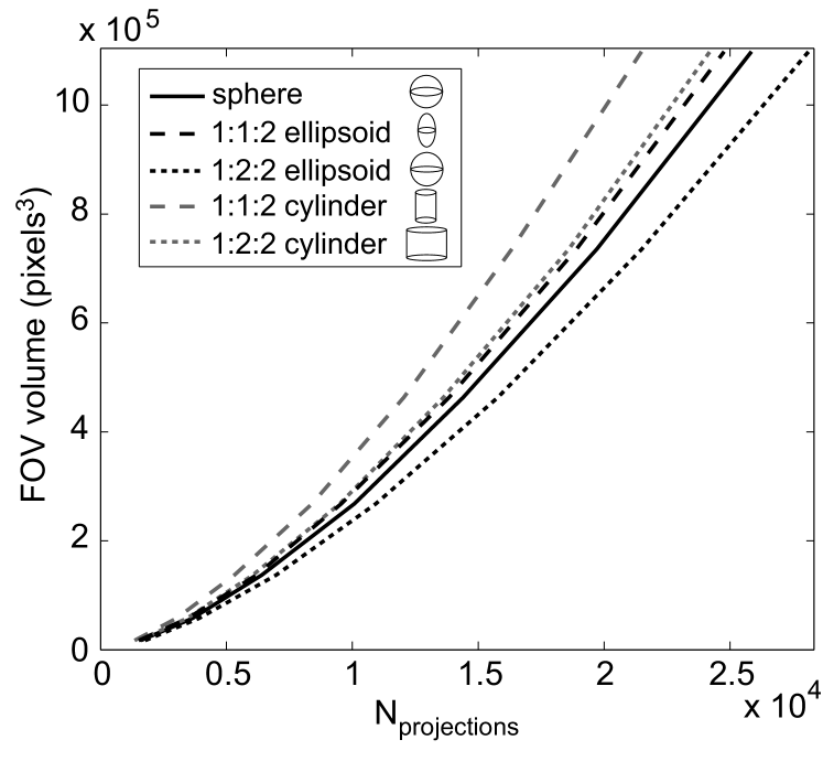
Figure 11: Number of projections for 3D anistropic FOV shapes, with ratios of $x$:$y$:$z$ lengths, versus the shape volume. All FOVs have 1 pixel isotropic resolution, and the curves shown are for both the cones-based and spiral-based design methods. Most of the anisotropic shapes are actually more efficient than the sphere, but at the cost of low-level aliasing within the FOV, seen in Fig. 9.

The scan volume efficiency for some 3D anisotropic FOV shapes is shown in Fig. 11. The anisotropic shapes are generally more efficient, although there is more variation in efficiency than in the 2D case (Fig. 7). The increased efficiency is at the expense of some low-level aliasing inside the FOV. The 1:1:2 ($x$:$y$:$z$) shapes only have anisotropy in the polar sampling, and they are more efficient than the 1:2:2 shapes that also have azimuthal sampling anisotropy. This difference is caused by the anisotropic $FOV_{\phi}$ cutting off portions of $FOV_{\theta}$, which can be seen in Fig. 4.

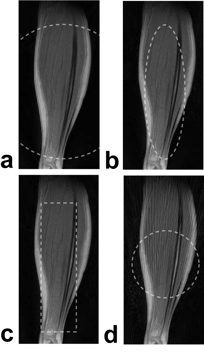
Figure 12: 2D PR Lower leg images with various FOV shapes, shown by the dashed lines. (a) 25 cm circular FOV requiring 393 projections, (b) 7.5 x 25 cm elliptical FOV requiring 197 projections, (c) 6.5 x 24 cm rectangular FOV requiring 195 projections, (d) 12.5 cm circular FOV requiring 196 projections. The non-circular FOV images (b,c) show no increase in aliasing artifacts or loss of resolution but were acquired with half the projections. The circular FOV acquired with half the projections (d) results in significant aliasing artifacts.

IV-C MRI Experiments

In vivo 2D PR leg images acquired with isotropic and anisotropic FOVs are shown in Fig. 12. The reduced FOV images (b-d) were acquired with half the number of projections as the full FOV image (a). The isotropic reduced FOV (d) results in significant streaking aliasing artifacts, while using anisotropic reduced FOVs tailored to the shape of the leg (b,c) results in no increase in artifact compared to the full isotropic FOV image. The images without aliasing (a-c) are all slightly undersampled, as shown by the overlaid FOV shapes, but no aliasing is visible due to the relatively diffuse aliasing pattern of PR.

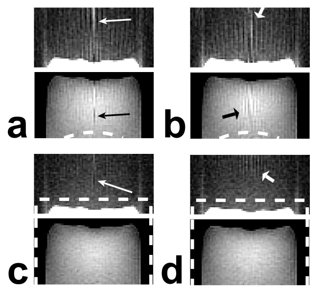
Figure 13: 3D PR phantom images, all acquired with the same number of projections. Isotropic FOV using the (a) cones-based method and (b) spiral-based method. Cylindrical FOV using the (c) cones-based method and (d) spiral-based method. The top images are all windowed identically to show the aliasing artifacts outside the bottle (white arrows). The bottom images are also identically windowed to show the aliasing artifacts within the bottle for the undersampled, isotropic FOVs (black arrows). The dashed lines indicate the supported FOV.

Figure 13 shows a representative slice from 3D PR acquisitions of a water bottle phantom using different FOVs, each with the same number of projections. In the isotropic FOV acquisitions, streaking artifacts are visible within the bottle and emanate from the edge of the bottle (arrows in Fig. 13a and b) because the FOV is not large enough. These artifacts have a peak amplitude of 23.2% of the signal for the cones-based design and 11.5% for the spiral-based design. By using a fully-sampled cylindrical FOV that matches the bottle’s shape, these streaks are completely shifted outside of the bottle. (arrows in Fig. 13c and d). The differences in aliasing diffusivity between the two 3D PR design methods, shown in the PSFs in Fig. 10, can also be seen in the images. There is a single, prominent aliasing streak when using the cones-based design (long, thin arrows), which is diffused with the spiral-based design (short, fat arrows), and the peak aliasing amplitudes also reflect this difference.

In vivo 3D PR images of a 3 cm abdomen slab acquired in a single breath-hold are shown in Figs. 14 and 15. The isotropic FOV images have significant streaking artifacts within the abdomen (arrows in Fig. 14a and 15a) because of the high undersampling ratios. Using a thin, squished cylindrical FOV tailored to the anatomy and the excited slab eliminates these streaking artifacts, as shown in Fig. 14b. A small degree of undersampling in this tailored FOV is also tolerated, as evidenced by the lack of streaking artifacts in Fig. 15b. The isotropic FOV streaking also results in a higher level of signal outside of the body in the axial images. More streaking is seen just outside the slab in the coronal images with the anisotropic FOV (arrows in Fig. 14b). This is expected because of the smaller superior-inferior dimension with the anisotropic FOV relative to the spherical FOV, for which the streaks in this dimension are outside of the displayed region. Acquiring a fully-sampled 36 cm isotropic FOV at 3 mm isotropic resolution requires 22656 projections, while an undersampled 19.6 cm FOV at 2 mm resolution requires 14744 projections, both of which are prohibitively large for single breath-hold imaging.

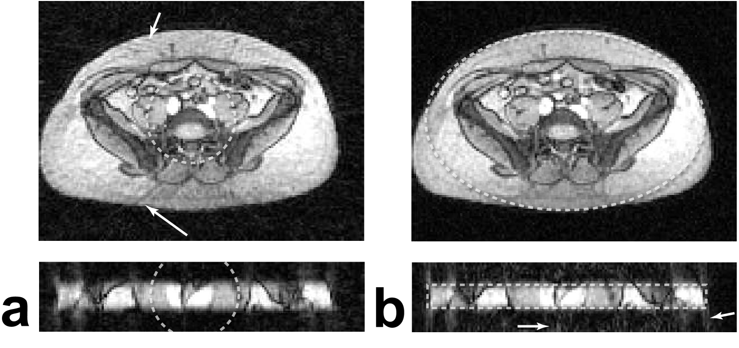
Figure 14: Axial (top) and coronal (bottom) slices from a thin-slab 3D PR abdomen data-set with 3 mm isotropic resolution acquired in a single breath-hold. (a) Isotropic 11.4 cm FOV requiring 2303 projections. (b) Cylindrical 36 x 23 x 3 cm FOV requiring 2368 projections. Both trajectories were designed using the spiral-based method. Streaking artifacts result from the high axial undersampling of the isotropic FOV (arrows in (a)). The tailored FOV eliminates these artifacts by reducing FOV in the slab dimension. This leads to the streaks in the coronal slice (arrows in (b)), but these are outside of the imaging volume.

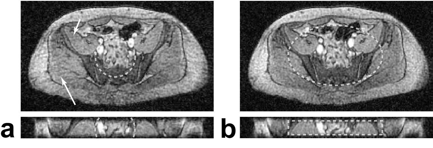
Figure 15: Same as Fig. 14, except with 2 mm isotropic resolution and increased undersampling. (a) Isotropic 8 cm FOV requiring 2519 projections. (b) Cylindrical 19.6 x 12.2 x 2.8 cm FOV requiring 2529 projections. The undersampled cylindrical FOV has no noticeable streaking artifacts (arrows), which obscure the anatomy with the isotropic FOV.

V Discussion

The algorithms presented are designed with fully-sampled FOV parameters, but will also be beneficial for undersampled radial imaging applications, as demonstrated in Fig. 15. For undersampled applications like VIPR [7], the desired FOV shape and size should be a scaled down version of the region-of-interest for equivalent undersampling factors in every dimension. The anisotropic FOV projections can also be applied to the highly constrained backprojection (HYPR) method for time-resolved MRI [24] because they can be reconstructed by filtered backprojection. Exam-specific FOVs can be used in all applications because the computation time of the design algorithms is small. Using an initial localizing scan, the desired FOV could be drawn or automatically detected and the acquisition tailored appropriately.

For some FOV and $k_{\rm max}$ shapes, the resulting PSFs have low-level aliasing within the desired FOV. This is due to the finite width of the aliasing lobes, as shown in Fig. 1b, which is not accounted for in our design algorithms. The projection angles are designed based on the peak at the center of these aliasing lobes, leaving the potential for up to half of the lobe to overlap inside the FOV. Overlap is more likely to occur as the radial separation of neighboring lobes increases, and thus is correlated with $\left|\frac{dFOV(\phi)}{d\phi}\right|$. The online animations of the PSFs show how the origin of the low-level aliasing is primarily along the longer edges where this derivative is the largest. This aliasing does not originate from minima or maxima of the FOV where the angular derivative is zero.

Narrower shapes, which have a larger angular derivative, have more desirable efficiency curves in Fig. 7 because they have more low-level aliasing within the FOV. For the shapes in Fig. 7, the total low-level aliasing power is approximately 0.60 and 1.3% of the main lobe power for the 1.5:1 and 2:1 ellipses, respectively, and 0.67, 0.91, and 1.2% for the 1:1, 1.5:1, and 2:1 rectangles. This confirms that narrower shapes have more low-level aliasing and that, in general, this aliasing is small.

There is no low-level aliasing in the dual shape sampling patterns seen in Fig. 8b, c, and d. This suggests that the low-level aliasing may be more correctly correlated with the derivative of $FOV(\phi)/k_{\rm max}(\phi+\frac{\pi}{2})$, which is zero for the dual shapes. This derivative is very large for the FOV and $k_{\rm max}$ shapes in Fig. 8e, which has significant aliasing inside the desired FOV. Another observation is that dual ellipse sampling can be formed by scaling an isotropic sampling pattern along one axis. By Fourier theory, this transformation scales the PSF along the corresponding axis by the inverse and introduces no low-level aliasing. It is possible that the other shapes may be formed by some transformation of isotropic case. We have found no derivation confirming this suggested low-level aliasing correlation or any general transformation starting with isotropic sampling.

With our method, it is possible to use 3D radial imaging trajectories to image thin slabs with isotropic resolution, as demonstrated in Figs. 14 and 15. Previously, this was achieved by using stacks of projections [6, 9], which lacks some of the benefits of a true 3D radial acquisition, such as ultra-short TEs. Stacking the projections also results in a coherent aliasing streak along the stacking direction, similar to the streak resulting from the cones-based design (see Fig. 10), which may be related to artifacts reported in the stacking dimension with contrast enhancement [7]. Both methods support one dimension of variable resolution, and stacks of 2D anisotropic FOV projections are also possible.

This projection design can also be applied to other centric-based k-space trajectories. It can be directly applied to twisting radial-line (TwiRL) trajectories [25] by specifying the angular spacing of the different acquisitions. Anisotropic resolution can also be incorporated by adjusting the twist in the radial line to match $k_{\rm max}(\phi)$. Interleaved spiral acquisitions can also be adjusted for anisotropic FOVs. The angular spacing of adjacent interleaves can be determined by our algorithm, and spirals with many interleaves will benefit the most from this adjustment. This could also be combined with the previous anisotropic FOV spiral method [26] which describes the design of the spirals themselves.

VI Conclusion

We have introduced a new method that designs projections for anisotropic FOVs in radial imaging. These FOVs can be precisely tailored to non-circular objects or regions-of-interest in 2D and 3D imaging. This allows for scan time reductions without introducing aliasing artifacts. For undersampled applications, this method allows for reduction of aliasing artifacts.

Algorithms have been presented for the design of 2D and 3D PR trajectories, as well as 3D cones. There is no loss in FOV area efficiency when using anisotropic FOVs. The algorithms are very simple and fast, allowing them to be computed on-the-fly. They also support variable trajectory extents which can be used in MRI to favor certain gradients or relax gradient constraints in 3D cones.

Appendix A Full-projection Spiral-based Design

For a spiral-based full-projection design, the spiralling path is sampled for $0\leq\theta\leq\frac{\pi}{2}$ by using $\theta_{\rm width}=\frac{\pi}{2}$ for the set of initial polar samples, and interpolating to $\hat{\Theta}[N_{polar}+1]=\frac{\pi}{2}$ and $\hat{K}_{\rm max}[N_{polar}+1]=k_{{\rm max},\theta}(\frac{\pi}{2})$. Near $\theta=\frac{\pi}{2}$, the polar sample spacing is not as desired because the opposite ends of the full-projections are spiralling in opposing directions. The spacing between these opposing turns varies approximately linearly from 1.5 to 0.5 times the desired spacing over each of the final two half-turns of the spiral. This spacing discrepancy also occurs with the isotropic 3D PR spiral design for full-projections[21]. This undersampling can be compensated for by adding an extra quarter-turn to the spiral. To do this, the interpolation is carried out to additional samples of $\hat{\Theta}[N_{polar}+2]=\frac{\pi}{2}+\frac{1}{4k_{{\rm max},\phi}FOV_{\theta}(\pi)}$ and $\hat{K}_{\rm max}[N_{polar}+2]=k_{{\rm max},\theta}(\hat{\Theta}[N_{polar}+2])$, with $N_{N_{polar}+1,{\rm est}}=\frac{N_{\phi,{\rm est}}}{4}$.

The density compensation must also be slightly modified to accomodate both the opposing spiral paths and the extra quarter-turn. Based on the 3D spiral geometry, it can be found that the total spacing from adjacent turns decreases approximately linearly between 1 and 0.5 times the desired spacing identically over the two last half-turns. Thus, the dcf from Eq. 21 is weighted over each of the half-turns separately by a linear ramp from 1 to 0.5 as $\theta$ increases.

References

- [1] P. C. Lauterbur, “Image formation by induced local interactions: Examples employing nuclear magnetic resonance,” Nature, vol. 242, pp. 190–191, May 1973.
- [2] P. Irarrazabal and D. G. Nishimura, “Fast three dimensional magnetic resonance imaging,” Magn Reson Med, vol. 33, no. 5, p. 656, May 1995.
- [3] P. T. Gurney, B. A. Hargreaves, and D. G. Nishimura, “Design and analysis of a practical 3D cones trajectory,” Magn Reson Med, vol. 55, no. 3, pp. 575–582, Mar. 2006.
- [4] G. H. Glover and J. M. Pauly, “Motion artifact reduction with projection reconstruction imaging,” Magn Reson Med, vol. 28, no. 2, pp. 275–289, Dec. 1992.
- [5] D. Nishimura, J. I. Jackson, and J. M. Pauly, “On the nature and reduction of the displacement artifact in flow images,” Magn Reson Med, vol. 22, no. 2, pp. 481–492, Dec. 1991.
- [6] D. C. Peters, F. R. Korosec, T. M. Grist, W. F. Block, J. E. Holden, K. K. Vigen, and C. A. Mistretta, “Undersampled projection reconstruction applied to MR angiography,” Magn Reson Med, vol. 43, no. 1, pp. 91–101, Jan. 2000.
- [7] A. V. Barger, W. F. Block, Y. Toropov, T. M. Grist, and C. A. Mistretta, “Time-resolved contrast-enhanced imaging with isotropic resolution and broad coverage using an undersampled 3D projection trajectory.” Magn Reson Med, vol. 48, no. 2, pp. 297–305, Aug. 2002.
- [8] A. Lu, E. Brodsky, T. M. Grist, and W. F. Block, “Rapid fat-suppressed isotropic steady-state free precession imaging using true 3D multiple-half-echo projection reconstruction,” Magn Reson Med, vol. 53, no. 3, pp. 692–699, Mar. 2005.
- [9] K. K. Vigen, D. C. Peters, T. M. Grist, W. F. Block, and C. A. Mistretta, “Undersampled projection-reconstruction imaging for time-resolved contrast-enhanced imaging,” Magn Reson Med, vol. 43, no. 2, pp. 170–176, Feb. 2000.
- [10] C. Stehning, P. Börnert, K. Nehrke, H. Eggers, and O. Dössel, “Fast isotropic volumetric coronary MR angiography using free-breathing 3D radial balanced FFE acquisition,” Magn Reson Med, vol. 52, no. 1, pp. 197–203, July 2004.
- [11] ——, “Free-breathing whole-heart coronary MRA with 3D radial SSFP and self-navigated image reconstruction,” Magn Reson Med, vol. 54, no. 2, pp. 476–480, Aug. 2005.
- [12] P. D. Gatehouse and G. M. Bydder, “Magnetic resonance imaging of short T2 components in tissue,” Clin Radiol, vol. 58, no. 1, pp. 1–19, Jan. 2003.
- [13] M. D. Robson, P. D. Gatehouse, M. Bydder, and G. M. Bydder, “Magnetic resonance: an introduction to ultrashort TE (UTE) imaging,” J Comput Assist Tomogr, vol. 27, no. 6, pp. 825–846, Nov./Dec. 2003.
- [14] J. Rahmer, P. Börnert, J. Groen, and C. Bos, “Three-dimensional radial ultrashort echo-time imaging with T2 adapted sampling,” Magn Reson Med, vol. 55, no. 5, pp. 1075–1082, May 2006.
- [15] P. E. Z. Larson, P. T. Gurney, K. Nayak, G. E. Gold, J. M. Pauly, and D. G. Nishimura, “Designing long-T2 suppression pulses for ultrashort echo time imaging,” Magn Reson Med, vol. 56, no. 1, pp. 94–103, July 2006.
- [16] T. Gu, F. R. Korosec, W. F. Block, S. B. Fain, Q. Turk, D. Lum, Y. Zhou, T. M. Grist, V. Haughton, and C. A. Mistretta, “PC VIPR: A high-speed 3D phase-contrast method for flow quantification and high-resolution angiography,” Am J Neuroradiol, vol. 26, no. 4, pp. 743–749, Apr. 2005.
- [17] K. Scheffler, “Tomographic imaging with nonuniform angular sampling,” J Comput Assist Tomogr, vol. 23, no. 1, pp. 162–166, Jan./Feb. 1999.
- [18] K. Scheffler and J. Hennig, “Reduced circular field-of-view imaging,” Magn Reson Med, vol. 40, no. 3, pp. 474–480, Sept. 1998.
- [19] M. L. Lauzon and B. K. Rutt, “Effects of polar sampling in k-space,” Magn Reson Med, vol. 36, no. 6, pp. 940–949, Dec. 1996.
- [20] G. H. Glover, J. M. Pauly, and K. M. Bradshaw, “Imaging 11B with a 3D projection reconstruction method,” J Magn Reson Imaging, vol. 2, no. 1, pp. 47–52, Jan./Feb. 1992.
- [21] S. T. S. Wong and M. S. Roos, “A strategy for sampling on a sphere applied to 3D selective RF pulse design,” Magn Reson Med, vol. 32, no. 6, pp. 778–784, Dec. 1994.
- [22] P. J. Beatty, D. G. Nishimura, and J. M. Pauly, “Rapid gridding reconstruction with a minimal oversampling ratio,” IEEE Trans Med Imaging, vol. 24, no. 6, pp. 799–808, June 2005.
- [23] C.-M. Tsai and D. Nishimura, “Reduced aliasing artifacts using variable-density -space sampling trajectories,” Magn Reson Med, vol. 43, no. 3, pp. 452–458, Mar. 2000.
- [24] C. A. Mistretta, O. Wieben, J. Velikina, W. Block, J. Perry, Y. Wu, K. Johnson, and Y. Wu, “Highly constrained backprojection for time-resolved MRI,” Magn Reson Med, vol. 55, no. 1, pp. 30–40, Jan. 2006.
- [25] J. I. Jackson, D. G. Nishimura, and A. Macovski, “Twisting radial lines with application to robust magnetic resonance imaging of irregular flow,” Magn Reson Med, vol. 25, no. 1, pp. 128–139, May 1992.
- [26] K. F. King, “Spiral scanning with anisotropic field of view,” Magn Reson Med, vol. 39, no. 3, pp. 448–456, Mar. 1998.