Abstract

Recent advances in probabilistic modelling have led to a large number of simulation-based inference algorithms which do not require numerical evaluation of likelihoods. However, a public benchmark with appropriate performance metrics for such ‘likelihood-free’ algorithms has been lacking. This has made it difficult to compare algorithms and identify their strengths and weaknesses. We set out to fill this gap: We provide a benchmark with inference tasks and suitable performance metrics, with an initial selection of algorithms including recent approaches employing neural networks and classical Approximate Bayesian Computation methods. We found that the choice of performance metric is critical, that even state-of-the-art algorithms have substantial room for improvement, and that sequential estimation improves sample efficiency. Neural network-based approaches generally exhibit better performance, but there is no uniformly best algorithm. We provide practical advice and highlight the potential of the benchmark to diagnose problems and improve algorithms. The results can be explored interactively on a companion website. All code is open source, making it possible to contribute further benchmark tasks and inference algorithms.

1 Introduction

Many domains of science, engineering, and economics make extensive use of models implemented as stochastic numerical simulators (Gourieroux et al., 1993; Ratmann et al., 2007; Alsing et al., 2018; Brehmer et al., 2018; Karabatsos and Leisen, 2018; Gonçalves et al., 2020). A key challenge when studying and validating such simulation-based models is the statistical identification of parameters which are consistent with observed data. In many cases, calculation of the likelihood is intractable or impractical, rendering conventional approaches inapplicable. The goal of simulation-based inference (SBI), also known as ‘likelihood-free inference’, is to perform Bayesian inference without requiring numerical evaluation of the likelihood function (Sisson et al., 2018; Cranmer et al., 2020). In SBI, it is generally not required that the simulator is differentiable, nor that one has access to its internal random variables.

In recent years, several new SBI algorithms have been developed (e.g., Gutmann and Corander, 2016; Papamakarios and Murray, 2016; Lueckmann et al., 2017; Chan et al., 2018; Greenberg et al., 2019; Papamakarios et al., 2019b; Prangle, 2019; Brehmer et al., 2020; Hermans et al., 2020; Järvenpää et al., 2020; Picchini et al., 2020; Rodrigues et al., 2020; Thomas et al., 2020), energized, in part, by advances in probabilistic machine learning (Rezende and Mohamed, 2015; Papamakarios et al., 2017, 2019a). Despite—or possibly because—of these rapid and exciting developments, it is currently difficult to assess how different approaches relate to each other theoretically and empirically: First, different studies often use different tasks and metrics for comparison, and comprehensive comparisons on multiple tasks and simulation budgets are rare. Second, some commonly employed metrics might not be appropriate or might be biased through the choice of hyperparameters. Third, the absence of a benchmark has made it necessary to reimplement tasks and algorithms for each new study. This practice is wasteful, and makes it hard to rapidly evaluate the potential of new algorithms. Overall, it is difficult to discern the most promising approaches and decide on which algorithm to use when. These problems are exacerbated by the interdisciplinary nature of research on SBI, which has led to independent development and co-existence of closely-related algorithms in different disciplines.

There are many exciting challenges and opportunities ahead, such as the scaling of these algorithms to high-dimensional data, active selection of simulations, and gray-box settings, as outlined in Cranmer et al. (2020). To tackle such challenges, researchers will need an extensible framework to compare existing algorithms and test novel ideas. Carefully curated, a benchmark framework will make it easier for researchers to enter SBI research, and will fuel the development of new algorithms through community involvement, exchange of expertise and collaboration. Furthermore, benchmarking results could help practitioners to decide which algorithm to use on a given problem of interest, and thereby contribute to the dissemination of SBI.

The catalyzing effect of benchmarks has been evident, e.g., in computer vision (Russakovsky et al., 2015), speech recognition (Hirsch and Pearce, 2000; Wang et al., 2018), reinforcement learning (Bellemare et al., 2013; Duan et al., 2016), Bayesian deep learning (Filos et al., 2019; Wenzel et al., 2020), and many other fields drawing on machine learning. Open benchmarks can be an important component of transparent and reproducible computational research. Surprisingly, a benchmark framework for SBI has been lacking, possibly due to the challenging endeavor of designing benchmarking tasks and defining suitable performance metrics.

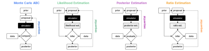
Figure 1: Overview of algorithms. We compare algorithms belonging to four distinct approaches to SBI: Classical ABC approaches as well as model-based approaches approximating likelihoods, posteriors, or density ratios. We contrast algorithms that use the prior distribution to propose parameters against ones that sequentially adapt the proposal. Classification and schemes following Cranmer et al. (2020).

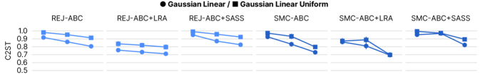
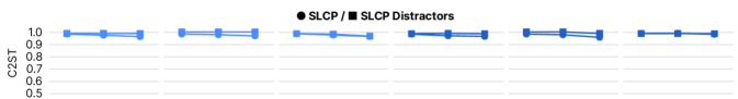
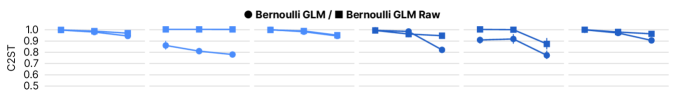
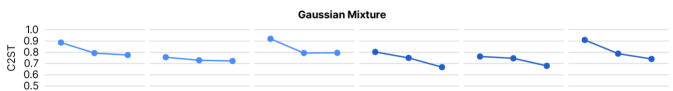
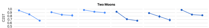
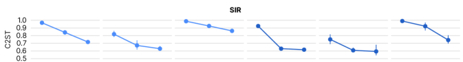
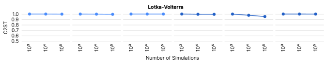
Figure 1: Additional ABC results with linear regression adjustment (LRA) and semi-automatic summary-statistics (SASS). We ran ABC with post-hoc LRA (Beaumont et al., 2002; Blum, 2018). On some tasks, this led to an improvement relative to versions without post-hoc adjustment. On Two Moons (bimodal posterior), linear adjustment decreased performance. We implemented our own SASS (Prangle et al., 2014b) with a third order polynomial feature expansion, and observed similar performance as with the implementation in abcpy toolbox (Dutta et al., 2017).

Here, we begin to address this challenge, and provide a benchmark framework for SBI to allow rapid and transparent comparisons of current and future SBI algorithms: First, we selected a set of initial algorithms representing distinct approaches to SBI (Fig. 1; Cranmer et al., 2020). Second, we analyzed multiple performance metrics which have been used in the SBI literature. Third, we implemented ten tasks including tasks popular in the field. The shortcomings of commonly used metrics led us to focus on tasks for which a likelihood can be evaluated, which allowed us to calculate reference (‘ground-truth’) posteriors. These reference posteriors are made available to allow rapid evaluation of SBI algorithms. Code for the framework is available at github.com/sbi-benchmark/sbibm and we maintain an interactive version of all results at sbi-benchmark.github.io.

The full potential of the benchmark will be realized when it is populated with additional community-contributed algorithms and tasks. However, our initial version already provides useful insights: 1) the choice of performance metric is critical; 2) the performance of the algorithms on some tasks leaves substantial room for improvement; 3) sequential estimation generally improves sample efficiency; 4) for small and moderate simulation budgets, neural-network based approaches outperform classical ABC algorithms, confirming recent progress in the field; and 5) there is no algorithm to rule them all. The performance ranking of algorithms is task-dependent, pointing to a need for better guidance or automated procedures for choosing which algorithm to use when. We highlight examples of how the benchmark can be used to diagnose shortcomings of algorithms and facilitate improvements. We end with a discussion of the limitations of the benchmark.

2 Benchmark

The benchmark consists of a set of algorithms, performance metrics and tasks. Given a prior $p(\boldsymbol{\mathbf{\theta}})$ over parameters $\boldsymbol{\mathbf{\theta}}$, a simulator to sample $\boldsymbol{\mathbf{x}}\sim p(\boldsymbol{\mathbf{x}}|\boldsymbol{\mathbf{\theta}})$ and an observation $\boldsymbol{\mathbf{x}}_{o}$, an algorithm returns an approximate posterior $q(\boldsymbol{\mathbf{\theta}}|\boldsymbol{\mathbf{x}}_{o})$, or samples from it, $\boldsymbol{\mathbf{\theta}}\sim q$. The approximate solution is tested, according to a performance metric, against a reference posterior $p(\boldsymbol{\mathbf{\theta}}|\boldsymbol{\mathbf{x}}_{o})$.

2.1 Algorithms

Following the classification introduced in the review by Cranmer et al. (2020), we selected algorithms addressing SBI in four distinct ways, as schematically depicted in Fig. 1. An important difference between algorithms is how new simulations are acquired: Sequential algorithms adaptively choose informative simulations to increase sample efficiency. While crucial for expensive simulators, it can require non-trivial algorithmic steps and hyperparameter choices. To evaluate whether the potential is realized empirically and justifies the algorithmic burden, we included sequential and non-sequential counterparts for algorithms of each category.

Keeping our initial selection focused allowed us to carefully consider implementation details and hyperparameters: We extensively explored performance and sensitivity to different choices in more than 10k runs, all results and details of which can be found in Appendix H. Our selection is briefly described below, full algorithm details are in Appendix A.

REJ-ABC and SMC-ABC. Approximate Bayesian Computation (ABC, Sisson et al., 2018) is centered around the idea of Monte Carlo rejection sampling (Tavaré et al., 1997; Pritchard et al., 1999). Parameters $\boldsymbol{\mathbf{\theta}}$ are sampled from a proposal distribution, simulation outcomes $\boldsymbol{\mathbf{x}}$ are compared with observed data $\boldsymbol{\mathbf{x}}_{o}$, and are accepted or rejected depending on a (user-specified) distance function and rejection criterion. While rejection ABC (REJ-ABC) uses the prior as a proposal distribution, the efficiency can be improved by using sequentially refined proposal distributions (SMC-ABC, Beaumont et al., 2002; Marjoram and Tavaré, 2006; Sisson et al., 2007; Toni et al., 2009; Beaumont et al., 2009). We implemented REJ-ABC with quantile-based rejection and used the scheme of Beaumont et al. (2009) for SMC-ABC. We extensively varied hyperparameters and compared the implementation of an ABC-toolbox (Klinger et al., 2018) against our own (Appendix H). We investigated linear regression adjustment (Blum and François, 2010) and the summary statistics approach by Prangle et al. (2014) (Suppl. Fig. 1).

NLE and SNLE. Likelihood estimation (or ‘synthetic likelihood’) algorithms learn an approximation to the intractable likelihood, for an overview see Drovandi et al. (2018). While early incarnations focused on Gaussian approximations (SL; Wood, 2010), recent versions utilize deep neural networks (Papamakarios et al., 2019b; Lueckmann et al., 2019) to approximate a density over $\boldsymbol{\mathbf{x}}$, followed by MCMC to obtain posterior samples. Since we primarily focused on these latter versions, we refer to them as neural likelihood estimation (NLE) algorithms, and denote the sequential variant with proposals as SNLE. In particular, we used the scheme proposed by Papamakarios et al. (2019b) which uses masked autoregressive flows (MAFs, Papamakarios et al., 2017) for density estimation. We improved MCMC sampling for (S)NLE and compared MAFs against Neural Spline Flows (NSFs; Durkan et al., 2019), see Appendix H.

NPE and SNPE. Instead of approximating the likelihood, these approaches directly target the posterior. Their origins date back to regression adjustment approaches (Blum and François, 2010). Modern variants (Papamakarios and Murray, 2016; Lueckmann et al., 2017; Greenberg et al., 2019) use neural networks for density estimation (approximating a density over $\boldsymbol{\mathbf{\theta}}$). Here, we used the recent algorithmic approach proposed by Greenberg et al. (2019) for sequential acquisitions. We report performance using NSFs for density estimation, which outperformed MAFs (Appendix H).

NRE and SNRE. Ratio Estimation approaches to SBI use classifiers to approximate density ratios (Izbicki et al., 2014; Pham et al., 2014; Cranmer et al., 2015; Dutta et al., 2016; Durkan et al., 2020; Thomas et al., 2020). Here, we used the recent approach proposed by Hermans et al. (2020) as implemented in Durkan et al. (2020): A neural network-based classifier approximates probability ratios and MCMC is used to obtain samples from the posterior. SNRE denotes the sequential variant of neural ratio estimation (NRE). In Appendix H we compare different classifier architectures for (S)NRE.

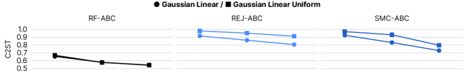
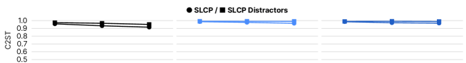
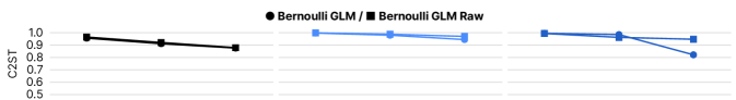
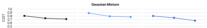
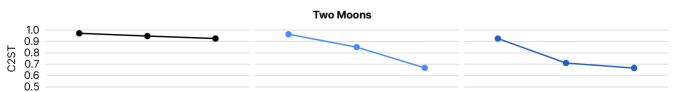
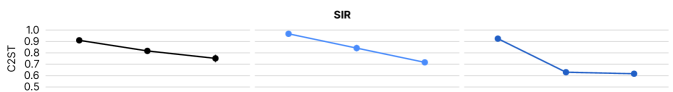
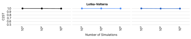
Figure 2: RF-ABC results. Results for RF-ABC (as described in A.9) compared to REJ-ABC and SMC-ABC on all benchmark tasks, using C2ST. Note that RF-ABC predicts each parameter individually, i.e. effectively assumes the posterior to be factorized– this is only appropriate for the Gaussian Linear, Gaussian Linear Uniform, and Gaussian Mixture tasks. On other tasks, the posterior deviates markedly from being factorized, and therefore it is to be expected that RF-ABC performance is limited, even when using many samples. Each data point corresponds to the mean and 95% confidence interval across 10 observations.

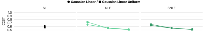
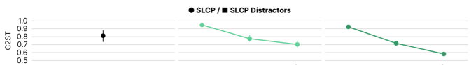
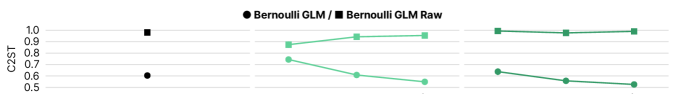
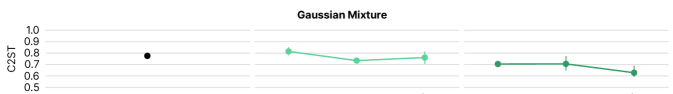
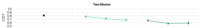
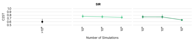
Figure 3: SL results. Results for SL compared to NLE and SNLE on benchmark tasks in terms of C2ST. Note that SL performs simulations at every MCMC step to approximate a Gaussian likelihood (see A.10 for details), and therefore it does not produce sensible results with the simulation budgets of other algorithms (between 1k and 100k), . In our experiments, SL required on the order of $10^{8}$ to $10^{9}$ simulations. For the SLCP Distractors and Lotka-Volterra stable estimation of covariances was not possible, which is why these tasks were omitted (details in A.10). We do not report SL results in the main paper, given the huge difference in simulation budget. Each data point corresponds to the mean and 95% confidence interval across 10 observations.

In addition, we benchmarked Random Forest ABC (RF-ABC; Raynal et al., 2019), a recent ABC variant, and Synthetic Likelihood (SL; Wood, 2010), mentioned above. However, RF-ABC only targets individual parameters (i.e. assumes posteriors to factorize), and SL requires new simulations for every MCMC step, thus requiring orders of magnitude more simulations than other algorithms. Therefore, we report results for these algorithms separately, in Suppl. Fig. 2 and Suppl. Fig. 3, respectively.

Algorithms can be grouped with respect to how their output is represented: 1) some return samples from the posterior, $\boldsymbol{\mathbf{\theta}}\sim q(\boldsymbol{\mathbf{\theta}}|\boldsymbol{\mathbf{x}}_{o})$ (REJ-ABC, SMC-ABC); 2) others return samples and allow evaluation of unnormalized posteriors $\tilde{q}(\boldsymbol{\mathbf{\theta}}|\boldsymbol{\mathbf{x}}_{o})$ ((S)NLE, (S)NRE); and 3) for some, the posterior density $q(\boldsymbol{\mathbf{\theta}}|\boldsymbol{\mathbf{x}}_{o})$ can be evaluated and sampled directly, without MCMC ((S)NPE). As discussed below, these properties constrain the metrics that can be used for comparison.

2.2 Performance metrics

Choice of a suitable performance metric is central to any benchmark. As the goal of SBI algorithms is to perform full inference, the ‘gold standard’ would be to quantify the similarity between the true posterior and the inferred one with a suitable distance (or divergence) measure on probability distributions. This would require both access to the ground-truth posterior, and a reliable means of estimating similarity between (potentially) richly structured distributions. Several performance metrics have been used in past research, depending on the constraints imposed by knowledge about ground-truth and the inference algorithm (see Table 1). In real-world applications, typically only the observation $\boldsymbol{\mathbf{x}}_{o}$ is known. However, in a benchmarking setting, it is reasonable to assume that one has at least access to the ground-truth parameters $\boldsymbol{\mathbf{\theta}}_{o}$. There are two commonly used metrics which only require $\boldsymbol{\mathbf{\theta}}_{o}$ and $\boldsymbol{\mathbf{x}}_{o}$, but suffer severe drawbacks for our purposes:

Probability $\boldsymbol{\mathbf{\theta}}_{o}$. The negative log probability of true parameters averaged over different $(\boldsymbol{\mathbf{\theta}}_{o},\boldsymbol{\mathbf{x}}_{o})$, $-\mathbb{E}[\log q(\boldsymbol{\mathbf{\theta}}_{o}|\boldsymbol{\mathbf{x}}_{o})]$, has been used extensively in the literature (Papamakarios and Murray, 2016; Durkan et al., 2018; Greenberg et al., 2019; Papamakarios et al., 2019b; Durkan et al., 2020; Hermans et al., 2020). Its appeal lies in the fact that one does not need access to the ground-truth posterior. However, using it only for a small set of $(\boldsymbol{\mathbf{\theta}}_{o},\boldsymbol{\mathbf{x}}_{o})$ is highly problematic: It is only a valid performance measure if averaged over a large set of observations sampled from the prior (Talts et al., 2018, detailed discussion including connection to simulation-based calibration in Appendix M). For reliable results, one would require inference for hundreds of $\boldsymbol{\mathbf{x}}_{o}$ which is only feasible if inference is rapid (amortized) and the density $q$ can be evaluated directly (among the algorithms used here this applies only to NPE).

Table 1: Applicability of metrics given knowledge about ground truth and algorithm. Whether a metric can be used depends on both what is known about the ground-truth of an inference task and what an algorithm returns: Information about ground truth can vary between just having observed data $\boldsymbol{\mathbf{x}}_{o}$ (typical setting in practice), knowing the generating parameter $\boldsymbol{\mathbf{\theta}}_{o}$, having posterior samples, gradients, or being able to evaluate the true posterior $p$. Tilde denotes unnormalized distributions. Access to information is cumulative.

	Ground truth $\rightarrow$
$\downarrow$  Algorithm	$\boldsymbol{\mathbf{x}}_{o}$	$\boldsymbol{\mathbf{\theta}}_{o}$	$\boldsymbol{\mathbf{\theta}}\sim p$	$\nabla\tilde{p}(\boldsymbol{\mathbf{\theta}}|\boldsymbol{\mathbf{x}}_{o})$	$p(\boldsymbol{\mathbf{\theta}}|\boldsymbol{\mathbf{x}}_{o})$
$\boldsymbol{\mathbf{\theta}}\sim q$	1	1	1, 3	1, 3, 4	1, 3, 4
$\tilde{q}(\boldsymbol{\mathbf{\theta}}|\boldsymbol{\mathbf{x}}_{o})$	1	1	1, 3	1, 3, 4	1, 3, 4
$q(\boldsymbol{\mathbf{\theta}}|\boldsymbol{\mathbf{x}}_{o})$	1	1, 2	1, 2, 3	1, 2, 3, 4	1, 2, 3, 4, 5

1 = PPCs, 2 = Probability $\boldsymbol{\mathbf{\theta}}_{0}$, 3 = 2-sample tests, 4 = 1-sample tests, 5 = $f$-divergences.

Posterior-Predictive Checks (PPCs). As the name implies, PPCs should be considered a mere check rather than a metric, although the median distance between predictive samples and $\boldsymbol{\mathbf{x}}_{o}$ has been reported in the SBI literature (Papamakarios et al., 2019b; Greenberg et al., 2019; Durkan et al., 2020). A failure mode of such a metric is that an algorithm obtaining a good MAP point estimate, could perfectly pass this check even if the estimated posterior is poor. Empirically, we found median-distances (MEDDIST) to be in disagreement with other metrics (see Results).

The shortcomings of these commonly-used metrics led us to focus on tasks for which it is possible to get samples from ground-truth posterior $\boldsymbol{\mathbf{\theta}}\sim p$, thus allowing us to use metrics based on two-sample tests:

Maximum Mean Discrepancy (MMD). MMD (Gretton et al., 2012; Sutherland et al., 2017) is a kernel-based 2-sample test. Recent papers (Papamakarios et al., 2019b; Greenberg et al., 2019; Hermans et al., 2020) reported MMD using translation-invariant Gaussian kernels with length scales determined by the median heuristic (Ramdas et al., 2015). We empirically found that MMD can be sensitive to hyperparameter choices, in particular on posteriors with multiple modes and length scales (see Results and Liu et al., 2020).

Classifier 2-Sample Tests (C2ST). C2STs (Friedman, 2004; Lopez-Paz and Oquab, 2017) train a classifier to discriminate samples from the true and inferred posteriors, which makes them simple to apply and easy to interpret. Therefore, we prefer to report and compare algorithms in terms of accuracy in classification-based tests. In the context of SBI, C2ST has e.g. been used in Gutmann et al. (2018); Dalmasso et al. (2020).

Other metrics that could be used include:

Kernelized Stein Discrepancy (KSD). KSD (Liu et al., 2016; Chwialkowski et al., 2016) is a 1-sample test, which require access to $\nabla_{\boldsymbol{\mathbf{\theta}}}\ \tilde{p}(\boldsymbol{\mathbf{\theta}}|\boldsymbol{\mathbf{x}}_{o})$ rather than samples from $p$ ($\tilde{p}$ is the unnormalized posterior). Like MMD, current estimators use translation-invariant kernels.

$f$-Divergences. Divergences such as Total Variation (TV) divergence and KL divergences can only be computed when the densities of true and approximate posteriors can be evaluated (Table 1). Thus, we did not use $f$-divergences for the benchmark.

Full discussion and details of metrics in Appendix M.

2.3 Tasks

The preceding considerations guided our selection of inference tasks: We focused on tasks for which reference posterior samples $\boldsymbol{\mathbf{\theta}}\sim p$ can be obtained, to allow calculation of 2-sample tests. We focused on eight purely statistical problems and two problems relevant in applied domains, with diverse dimensionalities of parameters and data (details in Appendix T):

Gaussian Linear/Gaussian Linear Uniform. We included two versions of simple, linear, 10-d Gaussian models, in which the parameter $\boldsymbol{\mathbf{\theta}}$ is the mean, and the covariance is fixed. The first version has a Gaussian (conjugate) prior, the second one a uniform prior. These tasks allow us to test how algorithms deal with trivial scaling of dimensionality, as well as truncated support.

SLCP/SLCP Distractors. A challenging inference task designed to have a simple likelihood and a complex posterior (Papamakarios et al., 2019b; Greenberg et al., 2019): The prior is uniform over five parameters $\boldsymbol{\mathbf{\theta}}$ and the data are a set of four two-dimensional points sampled from a Gaussian likelihood whose mean and variance are nonlinear functions of $\boldsymbol{\mathbf{\theta}}$. This induces a complex posterior with four symmetrical modes and vertical cut-offs. We included a second version with 92 additional, non-informative outputs (distractors) to test the ability to detect informative features.

Bernoulli GLM/Bernoulli GLM Raw. 10-parameter Generalized Linear Model (GLM) with Bernoulli observations. Inference was either performed on sufficient statistics (10-d) or raw data (100-d).

Gaussian Mixture. This inference task, introduced by Sisson et al. (2007), has become common in the ABC literature (Beaumont et al., 2009; Toni et al., 2009; Simola et al., 2020). It consists of a mixture of two two-dimensional Gaussian distributions, one with much broader covariance than the other.

Two Moons. A two-dimensional task with a posterior that exhibits both global (bimodality) and local (crescent shape) structure (Greenberg et al., 2019) to illustrate how algorithms deal with multimodality.

SIR. Dynamical systems represent paradigmatic use cases for SBI. SIR is an influential epidemiological model describing the dynamics of the number of individuals in three possible states: susceptible $S$, infectious $I$, and recovered or deceased, $R$. We infer the contact rate $\beta$ and the mean recovery rate $\gamma$, given observed infection counts $I$ at 10 evenly-spaced time points.

Lotka-Volterra. An influential model in ecology describing the dynamics of two interacting species, widely used in SBI studies. We infer four parameters $\boldsymbol{\mathbf{\theta}}$ related to species interaction, given the number of individuals in both populations at 10 evenly-spaced points in time.

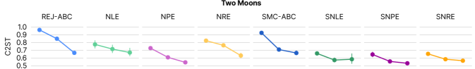
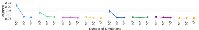
Figure 2: Performance on Two Moons according to various metrics. Best possible performance would be 0.5 for C2ST, 0 for MMD² and MEDDIST. Results for 10 observations each, means and 95% confidence intervals.

2.4 Experimental Setup

For each task, we sampled 10 sets of true parameters from the prior and generated corresponding observations $(\boldsymbol{\mathbf{\theta}}_{o},\boldsymbol{\mathbf{x}}_{o})_{1{:}10}$. For each observation, we generated 10k samples from the reference posterior. Some reference posteriors required a customised (likelihood-based) approach (Appendix B).

In SBI, it is typically assumed that total computation cost is dominated by simulation time. We therefore report performance at different simulation budgets. For each observation, each algorithm was run with a simulation budget ranging from 1k to 100k simulations.

For each run, we calculated metrics described above. To estimate C2ST accuracy, we trained a multilayer perceptron to tell apart approximate and reference posterior samples and performed five-fold cross-validation. We used two hidden layers, each with 10 times as many ReLu units as the dimensionality of the data. We also measured and report runtimes (Appendix R).

2.5 Software

Code. All code is released publicly at github.com/sbi-benchmark/sbibm. Our framework includes tasks, reference posteriors, metrics, plotting, and infrastructure tooling and is designed to be 1) easily extensible, 2) used with external toolboxes implementing algorithms. All tasks are implemented as probabilistic programs in Pyro (Bingham et al., 2019), so that likelihoods and gradients for reference posteriors can be extracted automatically. To make this possible for tasks that use ODEs, we developed a new interface between DifferentialEquations.jl (Rackauckas and Nie, 2017; Bezanson et al., 2017) and PyTorch (Paszke et al., 2019). In addition, specifying simulators in a probabilistic programming language has the advantage that ‘gray-box’ algorithms (Brehmer et al., 2020; Cranmer et al., 2020) can be added in the future. We here evaluated algorithms implemented in pyABC (Klinger et al., 2018), pyabcranger (Collin et al., 2020), and sbi (Tejero-Cantero et al., 2020). See Appendix B for details and existing SBI toolboxes.

Reproducibility. Instructions to reproduce experiments on cloud-based infrastructure are in Appendix B.

Website. Along with the code, we provide a web interface which allows interactive exploration of all the results (sbi-benchmark.github.io; Appendix W).

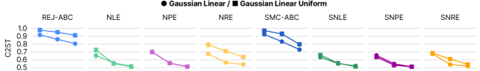
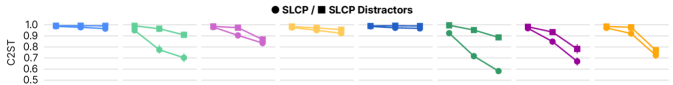
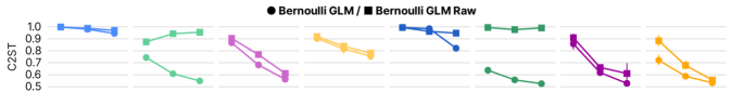
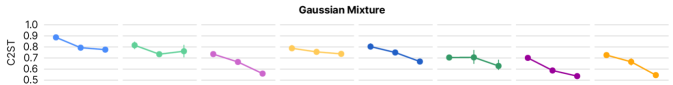
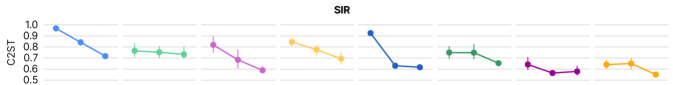
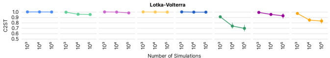
Figure 3: Performance on other benchmark tasks. Classification accuracy (C2ST) of REJ-ABC, SMC-ABC, NLE, SNLE, NPE, SNPE, NRE, SNRE for 10 observations each, means and 95% confidence intervals.

3 Results

We first consider empirical results on a single task, Two Moons, according to different metrics, which illustrate the following important insight:

#1: Choice of performance metric is key. While C2ST results on Two Moons show that performance increases with higher simulation budgets and that sequential algorithms outperform non-sequential ones for low to medium budgets, these results were not reflected in MMD and MEDDIST (Fig. 2): In our analyses, we found MMD to be sensitive to hyperparameter choices, in particular on tasks with complex posterior structure. When using the commonly employed median heuristic to set the kernel length scale on a task with multi-modal posteriors (like Two Moons), MMD had difficulty discerning markedly different posteriors. This can be ‘fixed’ by using hyperparameters adapted to the task (Suppl. Fig. 4). As discussed above, the median distance (though commonly used) can be ‘gamed’ by a good point estimate even if the estimated posterior is poor and is thus not a suitable performance metric. Computation of KSD showed numerical problems on Two Moons, due to the gradient calculation.

We assessed relationships between metrics empirically via the correlations across tasks (Suppl. Fig. 5). As discussed above, the log-probability of ground-truth parameters can be problematic when averaged over too few observations (e.g., 10, as is common in the literature): indeed, this metric had a correlation of only 0.3 with C2ST on Two Moons and 0.6 on the SLCP task. Based on these considerations, we used C2ST for reporting performance (Fig. 3; results for MMD, KSD and median distance on the website).

Based on the comparison of the performance across all tasks, we highlight the following main points:

#2: These are not solved problems. C2ST uses an interpretable scale (1 to 0.5), which makes it possible to conclude that, for several tasks, no algorithm could solve them with the specified budget (e.g., SLCP, Lotka-Volterra). This highlights that our problems—though conceptually simple—are challenging, and there is room for development of more powerful algorithms.

#3: Sequential estimation improves sample efficiency. Our results show that sequential algorithms outperform non-sequential ones (Fig. 3). The difference was small on simple tasks (i.e. linear Gaussian cases), yet pronounced on most others. However, we also found these methods to exhibit diminishing returns as the simulation budget grows, which points to an opportunity for future improvements.

#4: Density or ratio estimation-based algorithms generally outperform classical techniques. REJ-ABC and SMC-ABC were generally outperformed by more recent techniques which use neural networks for density- or ratio-estimation, and which can therefore efficiently interpolate between different simulations (Fig. 3). Without such model-based interpolation, even a simple 10-d Gaussian task can be challenging. However, classical rejection-based methods have a computational footprint that is orders of magnitudes smaller, as no network training is involved (Appendix R). Thus, on low-dimensional problems and for cheap simulators, these methods can still be competitive. See Suppl. Fig. 1 for results with additional ABC variants (Blum and François, 2010; Prangle et al., 2014) and Suppl. Fig. 2 for results on RF-ABC.

#5: No one algorithm to rule them all. Although sequential density or ratio estimation-based algorithms performed better than their non-sequential counterparts, there was no clear-cut answer as to which sequential method (SNLE, SNRE, and SNPE) should be preferred. To some degree, this is to be expected: these algorithms have distinct strengths that can play out differently depending on the problem structure (see discussions e.g., in Greenberg et al., 2019; Durkan et al., 2018, 2020). However, this has not been shown systematically before. We formulate some practical guidelines for choosing appropriate algorithms in Box 1.

#6: The benchmark can be used to diagnose implementation issues and improve algorithms. For example, (S)NLE and (S)NRE rely on MCMC sampling to compute posteriors, and this sampling step can limit the performance. Access to a reference posterior can help identify and improve such issues: We found that single chains initialized by sampling from the prior with axis-aligned slice sampling (as introduced in Papamakarios et al., 2019b) frequently got stuck in single modes. Based on this observation, we changed the MCMC strategy (details in Appendix A), which, though simple, yielded significant performance and speed improvements on the benchmark tasks. Similarly, (S)NLE and (S)NRE improved by transforming parameters to be unbounded: Without transformations, runs on some tasks can get stuck during MCMC sampling (e.g., Lotka-Volterra). While this is common advice for MCMC (Hogg and Foreman-Mackey, 2018), it has been lacking in code and papers of SBI approaches.

We used the benchmark to systematically compare hyperparameters: For example, as density estimators

Box 1: Practitioners’ advice for applying SBI algorithms. Based on our current results and understanding, we provide advice to practitioners seeking to apply SBI. There is no one-fits-all solution—which algorithm to use in practice will depend on the problem at hand. For additional advice, see Cranmer et al. (2020).

for (S)NLE and (S)NPE, we used NSFs (Durkan et al., 2020) which were developed after these algorithms were published. This revealed that higher capacity density estimators were beneficial for posterior but not likelihood estimation (detailed analysis in Appendix H).

These examples show how the benchmark makes it possible to diagnose problems and improve algorithms.

4 Limitations

Our benchmark, in its current form, has several limitations. First, the algorithms considered here do not cover the entire spectrum of SBI algorithms: We did not include sequential algorithms using active learning or Bayesian Optimization (Gutmann and Corander, 2016; Järvenpää et al., 2019; Lueckmann et al., 2019; Aushev et al., 2020), or ‘gray-box’ algorithms, which use additional information about or from the simulator (e.g., Baydin et al., 2019; Brehmer et al., 2020). We focused on approaches using neural networks for density estimation and did not compare to alternatives using Gaussian Processes (e.g., Meeds and Welling, 2014; Wilkinson, 2014). There are many other algorithms which the benchmark is currently lacking (e.g., Nott et al., 2014; Ong et al., 2018; Clarté et al., 2020; Prangle, 2019; Priddle et al., 2019; Picchini et al., 2020; Radev et al., 2020; Rodrigues et al., 2020). Keeping our initial selection small allowed us to carefully investigate hyperparameter choices. We focused on sequential algorithms with less sophisticated acquisition schemes and the black-box scenario, since we think these are important baselines for future comparisons.

Second, the tasks we considered do not cover the variety of possible challenges. Notably, while we have tasks with high dimensional data with and without structure, we have not included tasks with high-dimensional spatial structure, e.g., images. Such tasks would require algorithms that automatically learn summary statistics while exploring the structure of the data (e.g., Dinev and Gutmann, 2018; Greenberg et al., 2019; Hermans et al., 2020; Chen et al., 2021), an active research area.

Third, while we extensively investigated tuning choices and compared implementations, the results might nevertheless reflect our own areas of expertise.

Fourth, in line with common practice in SBI, results presented in the paper focused on performance as a function of the number of simulation calls. It is important to remember that differences in computation time can be substantial (see Appendix R): For example, (S)ABC was much faster than approaches requiring network training. Overall, sequential neural algorithms exhibited longest runtimes.

Fifth, for reasons described above, we focused on problems for which reference posteriors can be computed. This raises the question of how insights on these problems will generalize to ‘real-world’ simulators. Notably, even these simple problems already identify clear differences between, and limitations of, different SBI approaches. Since it is not possible to rigorously compare the performance of different algorithms directly on ‘real-world’ simulators due to the lack of appropriate metrics, we see the benchmark as a necessary stepping stone towards the development of (potentially automated) selection strategies for practical problems.

Sixth, in practice, the choice of algorithm can depend on aspects that are difficult to quantify: It will depend on the available information about a problem, the inference goal, and the speed of the simulator, among other considerations. We included some practical considerations and recommendations in Box 1.

Finally, benchmarking is an important tool, but not an end in itself—for example, conceptually new ideas might initially not yield competitive results but only reveal their true value later. Conversely, ‘overfitting’ on benchmarks can lead to the illusion of progress, and result in an undue focus on small implementation details which might not generalize beyond it. It would certainly be possible to cheat on this benchmark: In particular, as the simulators are available, one could use samples (or even likelihoods) to excessively tune hyperparameters for each task. This would hardly transfer to practice where such tuning is usually impossible (lack of metrics and expensive simulators). Therefore, we carefully compared choices and selected hyperparameters performing best across tasks (Appendix H).

5 Discussion

Quantitatively evaluating, comparing and improving algorithms through benchmarking is at the core of progress in machine learning. We here provided an initial benchmark for simulation-based inference. If used sensibly, it will be an important tool for clarifying and expediting progress in SBI. We hope that the current results on multiple widely-used algorithms already provide insights into the state of the field, assist researchers with algorithm development, and that our recommendations for practitioners will help them in selecting appropriate algorithms.

We believe that the full potential of the benchmark will be revealed as more researchers participate and contribute. To facilitate this process, and allow users to quickly explore and compare algorithms, we are providing precomputed reference posteriors, a website (sbi-benchmark.github.io), and open-source code (github.com/sbi-benchmark/sbibm).

Appendix A Algorithms

A.1 Rejection Approximate Bayesian Computation (REJ-ABC)

while in simulation budget do

       Sample $\boldsymbol{\mathbf{\theta}}^{\prime}$ from $p(\boldsymbol{\mathbf{\theta}})$

      Simulate data $\boldsymbol{\mathbf{x}}^{\prime}$ from $p(\boldsymbol{\mathbf{x}}|\boldsymbol{\mathbf{\theta}}^{\prime})$

      if $d(\boldsymbol{\mathbf{x}}^{\prime},\boldsymbol{\mathbf{x}}_{o})\leq\epsilon$ then

             Accept $\boldsymbol{\mathbf{\theta}}^{\prime}$

      else

             Reject $\boldsymbol{\mathbf{\theta}}^{\prime}$

       end if

      

end while

return Accepted samples $\{\boldsymbol{\mathbf{\theta}}^{\prime}\}$ from $\hat{p}(\boldsymbol{\mathbf{\theta}}|d(\boldsymbol{\mathbf{x}},\boldsymbol{\mathbf{x}}_{o})\leq\epsilon$)

Algorithm 1 Rejection ABC

Classical Approximate Bayesian Computation (ABC) is based on Monte Carlo rejection sampling (Tavaré et al., 1997; Pritchard et al., 1999): In rejection ABC, the evaluation of the likelihood is replaced by a comparison between observed data $\boldsymbol{\mathbf{x}}_{o}$ and simulated data $\boldsymbol{\mathbf{x}}$, based on a distance measure $d(\boldsymbol{\mathbf{x}},\boldsymbol{\mathbf{x}}_{o})$. Samples $\boldsymbol{\mathbf{\theta}}$ from the approximate posterior are obtained by collecting simulation parameters that result in simulated data that is close to the observed data.

More formally, given observed data $\boldsymbol{\mathbf{x}}_{o}$, a prior $p(\boldsymbol{\mathbf{\theta}})$ over parameters of simulation-based model $p(\boldsymbol{\mathbf{x}}|\boldsymbol{\mathbf{\theta}})$, a distance measure $d(\boldsymbol{\mathbf{x}},\boldsymbol{\mathbf{x}}_{o})$ and an acceptance threshold $\epsilon$, rejection ABC obtains parameter samples $\boldsymbol{\mathbf{\theta}}$ from the approximate posterior as outlined in Algorithm 1.

In theory, rejection ABC obtains samples from the true posterior $p(\boldsymbol{\mathbf{\theta}}|\boldsymbol{\mathbf{x}}_{o})$ in the limit $\epsilon\to 0$ and $N\to\infty$, where $N$ is the simulation budget. In practice, its accuracy depends on the trade-off between simulation budget and the rejection criterion $\epsilon$. Rejection ABC suffers from the curse of dimensionality, i.e., with linear increase in the dimensionality of $\boldsymbol{\mathbf{x}}$, an exponential increase in simulation budget is required to maintain accurate results.

For the benchmark, we did not use a fixed $\epsilon$-threshold, but quantile-based rejection. Depending on the simulation budget (1k, 10k, 100k), we used a quantile of (0.1, 0.01, or, 0.001), so that REJ-ABC returned 100 samples with smallest distance to $\boldsymbol{\mathbf{x}}_{o}$ in each of these cases (see Appendix H for different hyperparameter choices). In order to compute metrics on 10k samples, we sampled from a KDE fitted on the accepted parameters (details about KDE resampling in Appendix H). REJ-ABC requires the choice of the distance measure $d(\boldsymbol{\mathbf{x}},\boldsymbol{\mathbf{x}}_{o})$: here we used the $l_{2}$-norm.

A.2 Sequential Monte Carlo Approximate Bayesian Computation (SMC-ABC)

Set schedule $\boldsymbol{\mathbf{\epsilon}}$ (including initial $\epsilon_{0}$), population indicator $t=0$, and population size $N$

Initialize weights $W_{0}=1/N$ uniformly

Sample initial population $\{\boldsymbol{\mathbf{\theta}}_{0}^{(i)}\}$ using rejection sampling with $\epsilon_{0}$

while in simulation budget do

       Increase population indicator $t=t+1$

       Set particle indicator $i=0$

       while $i<N$ do

             Sample $\boldsymbol{\mathbf{\theta}}^{\prime}$ from previous population $\{\boldsymbol{\mathbf{\theta}}_{t-1}^{(i)}\}$ with weights $\{W_{t-1}^{(i)}\}$;

             Perturb $\boldsymbol{\mathbf{\theta}}^{\prime}$: $\boldsymbol{\mathbf{\theta}}^{\prime\prime}\sim K_{t}(\boldsymbol{\mathbf{\theta}}|\boldsymbol{\mathbf{\theta}}^{\prime})$

             Simulate data $x^{\prime\prime}$ from $p(\boldsymbol{\mathbf{x}}|\boldsymbol{\mathbf{\theta}}^{\prime\prime})$

             if $d(\boldsymbol{\mathbf{x}}^{\prime\prime},\boldsymbol{\mathbf{x}}_{o})\leq\epsilon_{t}$ then

                   Set $\boldsymbol{\mathbf{\theta}}_{t}^{(i)}=\boldsymbol{\mathbf{\theta}}^{\prime\prime}$ and $W_{t}^{i}=\frac{p(\boldsymbol{\mathbf{\theta}}_{t}^{(i)})}{\sum_{j=1}^{N}W_{t-1}^{j}K_{t}(\boldsymbol{\mathbf{\theta}}_{t}^{(i)}|\boldsymbol{\mathbf{\theta}}_{t-1}^{j})}$

                   Increase particle indicator $i=i+1$

                  

            else

                   reject $\boldsymbol{\mathbf{\theta}}^{\prime\prime}$

                  

             end if

            

       end while

      Normalize weights so that $\sum_{i}W_{t}^{(i)}=1$

      

end while

return Weighted samples $\{\boldsymbol{\mathbf{\theta}}_{t}^{(i)}\}$ from $\hat{p}(\boldsymbol{\mathbf{\theta}}|d(\boldsymbol{\mathbf{x}},\boldsymbol{\mathbf{x}}_{o})\leq\epsilon)$

Algorithm 2 Population Monte Carlo ABC (ABC-PMC) as in Beaumont et al. (2009)

Sequential Monte Carlo Approximate Bayesian Computation (SMC-ABC) algorithms (Beaumont et al., 2002; Marjoram and Tavaré, 2006; Sisson et al., 2007; Toni et al., 2009) are an extension of the classical rejection ABC approach, inspired by importance sampling and sequential Monte Carlo sampling. Central to SMC-ABC is the idea to approach the final set of samples from the approximate posterior by constructing a series of intermediate sets of samples slowly approaching the final set through perturbations.

Several variants have been developed (e.g., Sisson et al., 2007; Beaumont et al., 2009; Toni et al., 2009; Simola et al., 2020). Here, we used the scheme ABC-PMC scheme of Beaumont et al. (2009) and refer to it as SMC-ABC in the manuscript. More formally, the description of the ABC-PMC algorithm is as follows: Given observed data $\boldsymbol{\mathbf{x}}_{o}$, a prior $p(\boldsymbol{\mathbf{\theta}})$ over parameters of a simulation-based model $p(\boldsymbol{\mathbf{x}}|\boldsymbol{\mathbf{\theta}})$, a distance measure $d(\boldsymbol{\mathbf{x}},\boldsymbol{\mathbf{x}}_{o})$, a schedule of acceptance thresholds $\epsilon_{i}$, and a kernel $K(\boldsymbol{\mathbf{\theta}}|\boldsymbol{\mathbf{\theta}}^{\prime})$ to perturb intermediate samples, weighted samples of the approximate posterior are obtained as described in Algorithm 2.

SMC-ABC can improve the sampling efficiency compared to REJ-ABC and avoids severe inefficiencies due to a mismatch between initial sampling and the target distribution. However, it comes with more hyperparameters that can require careful tuning to the problem at hand, e.g., the choice of distance measure, kernel, and $\epsilon$-schedule. Like, REJ-ABC, SMC-ABC suffers from the curse of dimensionality.

For the benchmark, we considered the popular toolbox pyABC (Klinger et al., 2018). Additionally, to fully understand the details of the SMC-ABC approach, we also implemented our own version. In the main paper we report results obtained with our implementation because it yielded slightly better results. A careful comparison of the two approaches, and the optimization of hyperparameters like $\epsilon$-schedule, population size and perturbation kernel variance across different tasks are shown in Appendix H. After optimization, the crucial parameters of SMC-ABC were set to: $l_{2}$-norm as distance metric, quantile-based epsilon decay with 0.2 quantile, population size 100 for simulation budgets 1k and 10k, population size 1000 for simulation budget 100k, Gaussian perturbation kernel with empirical covariance from previous population scaled by 0.5. We obtained 10k samples required for calculation of metrics as follows: If a population is not complete within the simulation budget we completed it with accepted particles from the last population and recalculated all weights. We then fitted a KDE on all those particles and sampled 10k samples from the KDE.

A.3 Neural Likelihood Estimation (NLE)

Set $\mathcal{D}=\{\}$

for $n=1:N$ do

       Sample $\boldsymbol{\mathbf{\theta}}_{n}\sim p(\boldsymbol{\mathbf{\theta}})$

       Simulate $\boldsymbol{\mathbf{x}}_{n}\sim p(\boldsymbol{\mathbf{x}}|\boldsymbol{\mathbf{\theta}}_{n})$

       Add $(\boldsymbol{\mathbf{\theta}}_{n},\boldsymbol{\mathbf{x}}_{n})$ to $\mathcal{D}$

      

end for

Train $q_{\boldsymbol{\mathbf{\psi}}}(\boldsymbol{\mathbf{x}}|\boldsymbol{\mathbf{\theta}})$ on $\mathcal{D}$

return Samples from $\hat{p}(\boldsymbol{\mathbf{\theta}}|\boldsymbol{\mathbf{x}}_{o})\propto q_{\boldsymbol{\mathbf{\psi}}}(\boldsymbol{\mathbf{x}}_{o}|\boldsymbol{\mathbf{\theta}})p(\boldsymbol{\mathbf{\theta}})$ via MCMC; $q_{\boldsymbol{\mathbf{\psi}}}(\boldsymbol{\mathbf{x}}|\boldsymbol{\mathbf{\theta}})$

Algorithm 3 Single round Neural Likelihood as in Papamakarios et al. (2019b)

Likelihood estimation approaches to SBI use density estimation to approximate the likelihood $p(\boldsymbol{\mathbf{x}}_{o}|\boldsymbol{\mathbf{\theta}})$. After learning a surrogate $q_{\boldsymbol{\mathbf{\psi}}}$ ($\boldsymbol{\mathbf{\psi}}$ denoting the parameters of the estimator) for the likelihood function, one can for example use Markov Chain Monte Carlo (MCMC) based sampling algorithms to obtain samples from the approximate posterior $\hat{p}(\boldsymbol{\mathbf{\theta}}|\boldsymbol{\mathbf{x}}_{o})$. This idea dates back to using Gaussian approximations of the likelihood (Wood, 2010; Drovandi et al., 2018), and more recently, was extended to density estimation with neural networks (Papamakarios et al., 2019b; Lueckmann et al., 2019).

We refer to the single-round version of the (sequential) neural likelihood approach by Papamakarios et al. (2019b) as NLE, and outline it in Algorithm 3: Given a set of samples $\{\boldsymbol{\mathbf{\theta}}_{n},\boldsymbol{\mathbf{x}}_{n}\}_{1:N}$ obtained by sampling $\boldsymbol{\mathbf{\theta}}_{n}\sim p(\boldsymbol{\mathbf{\theta}})$ from the prior and simulating $\boldsymbol{\mathbf{x}}_{n}\sim p(\boldsymbol{\mathbf{x}}|\boldsymbol{\mathbf{\theta}}_{n})$, we train a conditional neural density estimator $q_{\boldsymbol{\mathbf{\psi}}}(\boldsymbol{\mathbf{x}}|\boldsymbol{\mathbf{\theta}})$ modelling the conditional of data given parameters on the set $\{\boldsymbol{\mathbf{\theta}}_{n},\boldsymbol{\mathbf{x}}_{n}\}_{1:N}$. Training proceeds by maximizing the log likelihood $\sum_{n}\log q_{\boldsymbol{\mathbf{\psi}}}(\boldsymbol{\mathbf{x}}|\boldsymbol{\mathbf{\theta}})$. Given enough simulations, a sufficiently flexible conditional neural density estimator approximates the likelihood in the support of the prior $p(\boldsymbol{\mathbf{\theta}})$ (Papamakarios et al., 2019b). Once $q_{\boldsymbol{\mathbf{\psi}}}$ is trained, samples from the approximate posterior $\hat{p}(\boldsymbol{\mathbf{\theta}}|\boldsymbol{\mathbf{x}}_{o})$ are obtained using MCMC sampling based on the approximate likelihood $\hat{p}(\boldsymbol{\mathbf{x}}_{o}|\boldsymbol{\mathbf{\theta}})$ and the prior $p(\boldsymbol{\mathbf{\theta}})$.

For MCMC sampling, Papamakarios et al. (2019b) suggest to use Slice Sampling (Neal, 2003) with a single chain. However, we observed that the accuracy of the obtained posterior samples can be substantially improved by changing the Slice Sampling scheme as follows: 1) Instead of a single chain, we used 100 parallel MCMC chains; 2) for initialization of the chains, we sampled 10k candidate parameters from the prior, evaluated them under the unnormalized approximate posterior, and used these values as weights to resample initial locations; 3) we transformed parameters to be unbounded as suggested e.g. in Bingham et al. (2019); Carpenter et al. (2017); Hogg and Foreman-Mackey (2018). In addition, we reimplemented the slice sampler to allow vectorized evaluations of the likelihood, which yielded significant computational speed-ups.

For the benchmark, we used as density estimator a Masked Autoregressive Flow (MAF, Papamakarios et al., 2017) with five flow transforms, each with two blocks and 50 hidden units, $\tanh$ non-linearity and batch normalization after each layer. For the MCMC step, we used the scheme as outlined above with 250 warm-up steps and ten-fold thinning, to obtain 10k samples from the approximate posterior (1k samples from each chain). In Appendix H we show results for all tasks obtained with a Neural Spline Flow (NSF, Durkan et al., 2019) for density estimation, using five flow transforms, two residual blocks of 50 hidden units each, ReLU non-linearity, and 10 bins.

A.4 Sequential Neural Likelihood Estimation (SNLE)

Set $\hat{p}_{0}(\boldsymbol{\mathbf{\theta}}|\boldsymbol{\mathbf{x}}_{o})=p(\boldsymbol{\mathbf{\theta}})$ and $\mathcal{D}=\{\}$

for r = 1 : R do

       for $n=1:N$ do

             Sample $\boldsymbol{\mathbf{\theta}}_{n}\sim\hat{p}_{r-1}(\boldsymbol{\mathbf{\theta}}|\boldsymbol{\mathbf{x}}_{o})$ with MCMC

             Simulate $\boldsymbol{\mathbf{x}}_{n}\sim p(\boldsymbol{\mathbf{x}}|\boldsymbol{\mathbf{\theta}}_{n})$

             Add $(\boldsymbol{\mathbf{\theta}}_{n},\boldsymbol{\mathbf{x}}_{n})$ to $\mathcal{D}$

            

       end for

      

      (Re-)train $q_{\boldsymbol{\mathbf{\psi}}}(\boldsymbol{\mathbf{x}}|\boldsymbol{\mathbf{\theta}})$ on $\mathcal{D}$

       Set $\hat{p}_{r}(\boldsymbol{\mathbf{\theta}}|\boldsymbol{\mathbf{x}}_{o})\propto q_{\boldsymbol{\mathbf{\psi}}}(\boldsymbol{\mathbf{x}}_{o}|\boldsymbol{\mathbf{\theta}})p(\boldsymbol{\mathbf{\theta}})$

      

end for

return Samples from $\hat{p}(\boldsymbol{\mathbf{\theta}}|\boldsymbol{\mathbf{x}}_{o})\propto q_{\boldsymbol{\mathbf{\psi}}}(\boldsymbol{\mathbf{x}}_{o}|\boldsymbol{\mathbf{\theta}})p(\boldsymbol{\mathbf{\theta}})$ via MCMC; $q_{\boldsymbol{\mathbf{\psi}}}(\boldsymbol{\mathbf{x}}|\boldsymbol{\mathbf{\theta}})$

Algorithm 4 Sequential Neural Likelihood as in Papamakarios et al. (2019b)

Sequential Neural Likelihood estimation (SNLE or SNL, Papamakarios et al., 2019b) extends the neural likelihood estimation approach described in the previous section to be sequential.

The idea behind sequential SBI algorithms is based on the following intuition: If for a particular inference problem, there is only a single $\boldsymbol{\mathbf{x}}_{o}$ one is interested in, then simulating data using parameters from the entire prior space might be inefficient, leading to a training set $\mathcal{D}$ that contains training data $(\boldsymbol{\mathbf{\theta}},\boldsymbol{\mathbf{x}})$ which carries little information about the posterior $p(\boldsymbol{\mathbf{\theta}}|\boldsymbol{\mathbf{x}}_{o})$. Instead, to increase sample efficiency, one may draw training data points from a proposal distribution $\tilde{p}(\boldsymbol{\mathbf{\theta}})$, ideally obtaining $\boldsymbol{\mathbf{\theta}}$ for which $\boldsymbol{\mathbf{x}}$ is close to $\boldsymbol{\mathbf{x}}_{o}$. One candidate that has been commonly used in the literature for such a proposal is the approximate posterior distribution itself.

SNLE is a multi-round version of NLE, where in each round new training samples are drawn from a proposal $\tilde{p}(\boldsymbol{\mathbf{\theta}})$. The proposal is chosen to be the posterior estimate at $\boldsymbol{\mathbf{x}}_{o}$ from the previous round $\hat{p}(\boldsymbol{\mathbf{\theta}}|\boldsymbol{\mathbf{x}}_{o})$ and its samples are obtained using MCMC. The proposal controls where $q_{\boldsymbol{\mathbf{\psi}}}(\boldsymbol{\mathbf{x}}|\boldsymbol{\mathbf{\theta}})$ is learned most accurately. Thus, by iterating over multiple rounds, a good approximation to the posterior can be learned more efficiently than by sampling all training data from the prior. SNLE is summarized in Algorithm 4.

For the benchmark, we used as density estimator a Masked Autoregressive Flow (Papamakarios et al., 2017), and MCMC to obtain posterior samples after every round, both with the same settings as described for NLE. The simulation budget was equally split across 10 rounds. In Appendix H, we show results for all tasks obtained with a Neural Spline Flow (NSF, Durkan et al., 2019) for density estimation, using five flow transforms, two residual blocks of 50 hidden units each, ReLU non-linearity, and 10 bins.

A.5 Neural Posterior Estimation (NPE)

for $j=1:N$ do

       Sample $\boldsymbol{\mathbf{\theta}}_{j}\sim p(\boldsymbol{\mathbf{\theta}})$

       Simulate $\boldsymbol{\mathbf{x}}_{j}\sim p(\boldsymbol{\mathbf{x}}|\boldsymbol{\mathbf{\theta}}_{j})$

      

end for

$\boldsymbol{\mathbf{\phi}}\leftarrow\operatorname*{arg\,min}\sum_{j}^{N}-\log q_{F(\boldsymbol{\mathbf{x}}_{j},\boldsymbol{\mathbf{\phi}})}(\boldsymbol{\mathbf{\theta}}_{j})$

Set $\hat{p}(\boldsymbol{\mathbf{\theta}}|\boldsymbol{\mathbf{x}}_{o})=q_{F(\boldsymbol{\mathbf{x}}_{o},\boldsymbol{\mathbf{\phi}})}(\boldsymbol{\mathbf{\theta}})$

return Samples from $\hat{p}(\boldsymbol{\mathbf{\theta}}|\boldsymbol{\mathbf{x}}_{o})$; $q_{F(\boldsymbol{\mathbf{x}},\boldsymbol{\mathbf{\phi}})}(\boldsymbol{\mathbf{\theta}})$

Algorithm 5 Single round Neural Posterior Estimation as in Papamakarios and Murray (2016)

NPE uses conditional density estimation to directly estimate the posterior. This idea dates back to regression adjustment approaches (Blum and François, 2010) and was extended to density estimators using neural networks (Papamakarios and Murray, 2016) more recently.

As outlined in Algorithm 5, the approach is as follows: Given a prior over parameters $p(\boldsymbol{\mathbf{\theta}})$ and a simulator, a set of training data points $(\boldsymbol{\mathbf{\theta}},\boldsymbol{\mathbf{x}})$ is generated. This training data is used to learn the parameters $\boldsymbol{\mathbf{\psi}}$ of a conditional density estimator $q_{\boldsymbol{\mathbf{\psi}}}(\boldsymbol{\mathbf{\theta}}|x)$ using a neural network $F(\boldsymbol{\mathbf{x}},\boldsymbol{\mathbf{\phi}})$, i.e., $\boldsymbol{\mathbf{\psi}}=F(\boldsymbol{\mathbf{x}},\boldsymbol{\mathbf{\phi}})$. The loss function is given by the negative log probability $-\log q_{\boldsymbol{\mathbf{\psi}}}(\boldsymbol{\mathbf{\theta}}|x)$. If the density estimator $q$ is flexible enough and training data is infinite, this loss function leads to perfect recovery of the ground-truth posterior (Papamakarios and Murray, 2016).

For the benchmark, we used the approach by Papamakarios and Murray (2016) with a Neural Spline Flow (NSF, Durkan et al., 2019) as density estimator, using five flow transforms, two residual blocks of 50 hidden units each, ReLU non-linearity, and 10 bins. We sampled 10k samples from the approximate posterior $q_{F(\boldsymbol{\mathbf{x}}_{o},\boldsymbol{\mathbf{\phi}})}(\boldsymbol{\mathbf{\theta}})$. In Appendix H, we compare NSFs to Masked Autoregressive Flows (MAFs, Papamakarios et al., 2017), as used in Greenberg et al. (2019); Durkan et al. (2020), with five flow transforms, each with two blocks and 50 hidden units, $\tanh$ non-linearity and batch normalization after each layer.

A.6 Sequential Neural Posterior Estimation (SNPE)

Set $\tilde{p}_{1}(\boldsymbol{\mathbf{\theta}})=p(\boldsymbol{\mathbf{\theta}})$

$c\leftarrow 0$

for $r=1:R$ do

       for $j=1:N$ do

             $c\leftarrow c+1$

             Sample $\boldsymbol{\mathbf{\theta}}_{c}\sim\tilde{p}_{r}(\boldsymbol{\mathbf{\theta}})$

             Simulate $\boldsymbol{\mathbf{x}}_{c}\sim p(\boldsymbol{\mathbf{x}}|\boldsymbol{\mathbf{\theta}}_{c})$

            

       end for

      $V_{r}(\Theta):=\begin{cases}\binom{c}{M}^{-1}&\text{ if }\Theta=\{\boldsymbol{\mathbf{\theta}}_{b_{1}},\boldsymbol{\mathbf{\theta}}_{b_{1}},\ldots,\boldsymbol{\mathbf{\theta}}_{b_{M}}\}\text{ and }1\leq b_{1}<b_{2}<\ldots<b_{M}\leq c\\ 0&\text{ otherwise}\end{cases}$

      

      $\boldsymbol{\mathbf{\phi}}\leftarrow\operatorname*{arg\,min}_{\boldsymbol{\mathbf{\phi}}}\mathbb{E}_{\Theta\sim V_{r}(\Theta)}\left[\sum_{\boldsymbol{\mathbf{\theta}}_{j}\in\Theta}-\log\tilde{q}_{\boldsymbol{\mathbf{x}}_{j},\boldsymbol{\mathbf{\phi}}}(\boldsymbol{\mathbf{\theta}}_{j})\right]$

       Set $\tilde{p}_{r+1}(\boldsymbol{\mathbf{\theta}}):=q_{F(\boldsymbol{\mathbf{x}}_{o},\boldsymbol{\mathbf{\phi}})}(\boldsymbol{\mathbf{\theta}})$

      

end for

return Samples from $\hat{p}_{R}(\boldsymbol{\mathbf{\theta}}|\boldsymbol{\mathbf{x}}_{o})$; $q_{F(x,\boldsymbol{\mathbf{\phi}})}(\boldsymbol{\mathbf{\theta}})$

Algorithm 6 Sequential Neural Posterior Estimation with atomic proposals (Greenberg et al., 2019)

Sequential Neural Posterior Estimation SNPE is the sequential analog of NPE, and meant to increase sample efficiency (see also subsection A.4). When the posterior is targeted directly, using a proposal distribution $\tilde{p}(\boldsymbol{\mathbf{\theta}})$ different from the prior requires a correction step—without it, the posterior under the proposal distribution would be inferred (Papamakarios and Murray, 2016). This so-called proposal posterior is denoted by $\tilde{p}(\boldsymbol{\mathbf{\theta}}|\boldsymbol{\mathbf{x}})$:

$$\tilde{p}(\boldsymbol{\mathbf{\theta}}|\boldsymbol{\mathbf{x}}) =p(\boldsymbol{\mathbf{\theta}}|\boldsymbol{\mathbf{x}})\frac{\tilde{p}(\boldsymbol{\mathbf{\theta}})p(\boldsymbol{\mathbf{x}})}{p(\boldsymbol{\mathbf{\theta}})\tilde{p}(\boldsymbol{\mathbf{x}})},$$

where $\tilde{p}(\boldsymbol{\mathbf{x}})=\int_{\boldsymbol{\mathbf{\theta}}}\tilde{p}(\boldsymbol{\mathbf{\theta}})p(\boldsymbol{\mathbf{x}}|\boldsymbol{\mathbf{\theta}})$. Note that for $\tilde{p}(\boldsymbol{\mathbf{\theta}})=p(\boldsymbol{\mathbf{\theta}})$, it directly follows that $\tilde{p}(\boldsymbol{\mathbf{\theta}}|\boldsymbol{\mathbf{x}})=p(\boldsymbol{\mathbf{\theta}}|\boldsymbol{\mathbf{x}})$.

There have been three different approaches to this correction step so far, leading to three versions of SNPE (Papamakarios and Murray, 2016; Lueckmann et al., 2017; Greenberg et al., 2019). All three algorithms have in common that they train a neural network $F(\boldsymbol{\mathbf{x}},\boldsymbol{\mathbf{\phi}})$ to learn the parameters of a family of densities $q_{\boldsymbol{\mathbf{\psi}}}$ to estimate the posterior. They differ in what is targeted by $q_{\boldsymbol{\mathbf{\psi}}}$ and which loss is used for $F$.

SNPE-A (Papamakarios and Murray, 2016) trains $F$ to target the proposal posterior $\tilde{p}(\boldsymbol{\mathbf{\theta}}|\boldsymbol{\mathbf{x}})$ by minimizing the log likelihood loss $-\sum_{n}\log q_{\boldsymbol{\mathbf{\psi}}}(\boldsymbol{\mathbf{\theta}}_{n}|\boldsymbol{\mathbf{x}}_{n})$, and then post-hoc solves for $p(\boldsymbol{\mathbf{\theta}}|\boldsymbol{\mathbf{x}})$. The analytical post-hoc step places restrictions on $q_{\boldsymbol{\mathbf{\psi}}}$, the proposal, and prior. Papamakarios and Murray (2016) used Gaussian mixture density networks, single Gaussians proposals, and Gaussian or uniform priors. SNPE-B (Lueckmann et al., 2017) trains $F$ with the importance weighted loss $-\sum_{n}\frac{p(\boldsymbol{\mathbf{\theta}}_{n}}{\tilde{p}(\boldsymbol{\mathbf{\theta}}_{n})}\log q_{\boldsymbol{\mathbf{\psi}}}(\boldsymbol{\mathbf{\theta}}_{n}|\boldsymbol{\mathbf{x}}_{n})$ to directly recover $p(\boldsymbol{\mathbf{\theta}}|\boldsymbol{\mathbf{x}})$ without the need for post-hoc correction, removing restrictions with respect to $q_{\boldsymbol{\mathbf{\psi}}}$, the proposal, and prior. However, the importance weights can have high variance during training, leading to inaccurate inference for some tasks (Greenberg et al., 2019). SNPE-C (APT) (Greenberg et al., 2019) alleviates this issue by reparameterizing the problem such that it can infer the posterior by maximizing an estimated proposal posterior. It trains $F$ to approximate $p(\boldsymbol{\mathbf{\theta}}|\boldsymbol{\mathbf{x}})$ with $q_{F(\boldsymbol{\mathbf{x}},\boldsymbol{\mathbf{\phi}})}(\boldsymbol{\mathbf{\theta}})$, using a loss defined on the approximate proposal posterior $\tilde{q}_{\boldsymbol{\mathbf{x}},\boldsymbol{\mathbf{\phi}}}(\boldsymbol{\mathbf{\theta}})$. Greenberg et al. (2019) introduce ‘atomic’ proposals to allow for arbitrary choices of the density estimator, e.g., flows (Papamakarios et al., 2019a): The loss on $\tilde{q}_{\boldsymbol{\mathbf{x}},\boldsymbol{\mathbf{\phi}}}(\boldsymbol{\mathbf{\theta}})$ is calculated as the expectation over proposal sets $\Theta$ sampled from a so-called ‘hyperproposal’ $V(\Theta)$ as outlined in Algorithm 6 (see Greenberg et al., 2019, for full details).

For the benchmark, we used the approach by Greenberg et al. (2019) with ‘atomic’ proposals and referred to it as SNPE. As density estimator, we used a Neural Spline Flow (Durkan et al., 2019) with the same settings as for NPE. For the ‘atomic’ proposals, we used $M=10$ atoms (larger $M$ was too demanding in terms of memory). The simulation budget was equally split across 10 rounds and for the final round, we obtained 10k samples from the approximate posterior $\hat{p}_{R}(\boldsymbol{\mathbf{\theta}}|\boldsymbol{\mathbf{x}}_{o})$. In Appendix H, we compare NSFs to Masked Autoregressive Flows (MAFs, Papamakarios et al., 2017), as used in Greenberg et al. (2019); Durkan et al. (2020), with five flow transforms, each with two blocks and 50 hidden units, $\tanh$ non-linearity and batch normalization after each layer.

A.7 Neural Ratio Estimation (NRE)

Set optimization criterion $l$ (e.g., BCE)

for $j=1:N$ do

       Sample $\boldsymbol{\mathbf{\theta}}_{j}\sim p(\boldsymbol{\mathbf{\theta}})$

       Sample $\boldsymbol{\mathbf{\theta}}_{j}^{\prime}\sim p(\boldsymbol{\mathbf{\theta}})$

       Simulate $\boldsymbol{\mathbf{x}}_{j}\sim p(\boldsymbol{\mathbf{x}}|\boldsymbol{\mathbf{\theta}}_{j})$

      

end for

$\boldsymbol{\mathbf{\phi}}\leftarrow\operatorname*{arg\,min}l(d_{\boldsymbol{\mathbf{\phi}}}(\boldsymbol{\mathbf{x}}_{n},\boldsymbol{\mathbf{\theta}}_{n}),1)+l(d_{\boldsymbol{\mathbf{\phi}}}(\boldsymbol{\mathbf{x}}_{n},\boldsymbol{\mathbf{\theta}}_{n}^{\prime}),0)$

Parameterize $d_{\boldsymbol{\mathbf{\phi}}}(\boldsymbol{\mathbf{x}},\boldsymbol{\mathbf{\theta}})$

return Samples from $\hat{p}(\boldsymbol{\mathbf{\theta}}|\boldsymbol{\mathbf{x}}_{o})$ via MCMC; $d_{\boldsymbol{\mathbf{\phi}}}(\boldsymbol{\mathbf{x}},\boldsymbol{\mathbf{\theta}})$

Algorithm 7 Single round Neural Ratio Estimation as in Hermans et al. (2020)

Neural ratio estimation (NRE) uses neural-network based classifiers to approximate the posterior $p(\boldsymbol{\mathbf{\theta}}|\boldsymbol{\mathbf{x}}_{o})$. While neural-network based approaches described in the previous sections use density estimation to either estimate the likelihood ((S)NLE) or the posterior ((S)NPE), NRE algorithms ((S)NRE) use classification to estimate a ratio of likelihoods. The ratio can then be used for posterior evaluation or MCMC-based sampling.

Likelihood ratio estimation can be used for SBI because it allows to perform MCMC without evaluating the intractable likelihood. In MCMC, the transition probability from a current parameter $\boldsymbol{\mathbf{\theta}}_{t}$ to a proposed parameter $\boldsymbol{\mathbf{\theta}}^{\prime}$ depends on the posterior ratio and in turn on the likelihood ratio between the two parameters:

$$\frac{p(\boldsymbol{\mathbf{\theta}}^{\prime}|\boldsymbol{\mathbf{x}})}{p(\boldsymbol{\mathbf{\theta}}_{t}|\boldsymbol{\mathbf{x}})} =\frac{p(\boldsymbol{\mathbf{\theta}}^{\prime})p(\boldsymbol{\mathbf{x}}|\boldsymbol{\mathbf{\theta}}^{\prime})/p(\boldsymbol{\mathbf{x}})}{p(\boldsymbol{\mathbf{\theta}}_{t})p(\boldsymbol{\mathbf{x}}|\boldsymbol{\mathbf{\theta}}_{t})/p(\boldsymbol{\mathbf{x}})}=\frac{p(\boldsymbol{\mathbf{\theta}}^{\prime})p(\boldsymbol{\mathbf{x}}|\boldsymbol{\mathbf{\theta}}^{\prime})}{p(\boldsymbol{\mathbf{\theta}}_{t})p(\boldsymbol{\mathbf{x}}|\boldsymbol{\mathbf{\theta}}_{t})}.$$

Therefore, given a ratio estimator $r(\boldsymbol{\mathbf{x}}|\boldsymbol{\mathbf{\theta}}^{\prime},\boldsymbol{\mathbf{\theta}}_{t})=\frac{p(\boldsymbol{\mathbf{x}}|\boldsymbol{\mathbf{\theta}}^{\prime})}{p(\boldsymbol{\mathbf{x}}|\boldsymbol{\mathbf{\theta}}_{t})}$ learned from simulations, one can perform MCMC to obtain samples from the posterior, even if evaluating $p(\boldsymbol{\mathbf{x}}|\boldsymbol{\mathbf{\theta}})$ is intractable.

Hermans et al. (2020) proposed the following approach for MCMC with classifiers to approximate density ratios: A classifier is trained to distinguish samples from an arbitrary $(\boldsymbol{\mathbf{\theta}},\boldsymbol{\mathbf{x}})\sim p(\boldsymbol{\mathbf{x}}|\boldsymbol{\mathbf{\theta}})p(\boldsymbol{\mathbf{\theta}})$ and samples from the marginal model $(\boldsymbol{\mathbf{\theta}},\boldsymbol{\mathbf{x}})\sim p(\boldsymbol{\mathbf{\theta}})p(\boldsymbol{\mathbf{x}})$. This results in a likelihood-to-evidence estimator that needs to be trained only once to be evaluated for any $\boldsymbol{\mathbf{\theta}}$. The training of the classifier $d_{\boldsymbol{\mathbf{\phi}}}(\boldsymbol{\mathbf{x}},\boldsymbol{\mathbf{\theta}})$ proceeds by minimizing the binary cross-entropy loss (BCE), as outlined in Algorithm 7. Once the classifier $d_{\boldsymbol{\mathbf{\phi}}}(\boldsymbol{\mathbf{x}},\boldsymbol{\mathbf{\theta}})$ is parameterized, it can be used to perform MCMC to obtain samples from the posterior. The authors name their approach Amortized Approximate Likelihood Ratio MCMC (AALR-MCMC): It is amortized because once the likelihood ratio estimator is trained, it is possible to run MCMC for any $\boldsymbol{\mathbf{x}}\sim p(\boldsymbol{\mathbf{x}})$.

Earlier ratio estimation algorithms for SBI (e.g., Izbicki et al., 2014; Pham et al., 2014; Cranmer et al., 2015; Dutta et al., 2016) and their connections to recent methods are discussed in Thomas et al. (2020), as well as in Durkan et al. (2020). AALR-MCMC is closely related to LFIRE (Dutta et al., 2016) but trains an amortized classifier rather than a separate one per posterior evaluation. Durkan et al. (2020) showed that the loss of AALR-MCMC is closely related to the atomic SNPE-C/APT approach of Greenberg et al. (2019) (SNPE) and that both can be combined in a unified framework. Durkan et al. (2020) changed the formulation of the loss function for training the classifier from binary to multi-class.

For the benchmark, we used neural ratio estimation (NRE) as formulated by Durkan et al. (2020) and implemented in the sbi toolbox (Tejero-Cantero et al., 2020). As a classifier, we used a residual network architecture (ResNet) with two hidden layers of 50 units and ReLU non-linearity, trained with Adam (Kingma and Ba, 2015). Following the notation of Durkan et al. (2020), we used $K=10$ as the size of the contrasting set. For the MCMC step, we followed the same procedure as described for NLE, i.e., using Slice Sampling with 100 chains, to obtain 10k samples from each approximate posterior. In Appendix H, we show results for all tasks obtained with a multi-layer perceptron (MLP) architecture with two hidden layers of 50 ReLu units, and batch normalization.

A.8 Sequential Neural Ratio Estimation (SNRE)

Set optimization criterion $l$ (e.g., BCE)

Set $\tilde{p}(\boldsymbol{\mathbf{\theta}})=p(\boldsymbol{\mathbf{\theta}})$

for $r=1:R$ do

       for $j=1:N$ do

             Sample $\boldsymbol{\mathbf{\theta}}_{j}\sim\tilde{p}(\boldsymbol{\mathbf{\theta}})$ (via $d_{\boldsymbol{\mathbf{\phi}}}$ and MCMC)

             Sample $\boldsymbol{\mathbf{\theta}}_{j}^{\prime}\sim\tilde{p}(\boldsymbol{\mathbf{\theta}})$ (via $d_{\boldsymbol{\mathbf{\phi}}}$ and MCMC)

             Simulate $\boldsymbol{\mathbf{x}}_{j}\sim p(\boldsymbol{\mathbf{x}}|\boldsymbol{\mathbf{\theta}}_{j})$

            

       end for

      $\boldsymbol{\mathbf{\phi}}\leftarrow\operatorname*{arg\,min}l(I^{\prime}n,\boldsymbol{\mathbf{\theta}}_{n}),1)+l(d_{\boldsymbol{\mathbf{\phi}}}(\boldsymbol{\mathbf{x}}_{n},\boldsymbol{\mathbf{\theta}}_{n}^{\prime}),0)$;

       Parameterize $d_{\boldsymbol{\mathbf{\phi}}}(\boldsymbol{\mathbf{x}},\boldsymbol{\mathbf{\theta}})$

      

end for

return Samples from $\hat{p}(\boldsymbol{\mathbf{\theta}}|\boldsymbol{\mathbf{x}}_{o})$ via MCMC; $d_{\boldsymbol{\mathbf{\phi}}}(\boldsymbol{\mathbf{x}},\boldsymbol{\mathbf{\theta}})$

Algorithm 8 Sequential Neural Ratio Estimation as in Hermans et al. (2020)

Sequential Neural Ratio Estimation (SNRE) is the sequential version of NRE, and meant to increase sample efficiency, at the cost of needing to train new classifiers for different $\boldsymbol{\mathbf{x}}_{o}$.

A sequential version of neural ratio estimation was proposed by Hermans et al. (2020). As with other sequential algorithms, the idea is to replace the prior by a proposal distribution $\tilde{p}(\boldsymbol{\mathbf{\theta}})$ that is focused on $\boldsymbol{\mathbf{x}}_{o}$ in the sense that the sampled parameters $\boldsymbol{\mathbf{\theta}}$ result in simulated data $\boldsymbol{\mathbf{x}}$ that are informative about $\boldsymbol{\mathbf{x}}_{o}$. The proposal for the next round is the posterior estimate from the previous round. The ratio estimator then becomes $\tilde{r}(\boldsymbol{\mathbf{x}},\boldsymbol{\mathbf{\theta}})$ and is refined over rounds by training the underlying classifier with positive examples $(\boldsymbol{\mathbf{x}},\boldsymbol{\mathbf{\theta}})\sim p(\boldsymbol{\mathbf{x}}|\boldsymbol{\mathbf{\theta}})\tilde{p}(\boldsymbol{\mathbf{\theta}})$ and negative examples $(\boldsymbol{\mathbf{x}},\boldsymbol{\mathbf{\theta}})\sim p(\boldsymbol{\mathbf{x}})\tilde{p}(\boldsymbol{\mathbf{\theta}})$. Exact posterior evaluation is not possible anymore, but samples can be obtained as before via MCMC. These steps are outlined in Algorithm 8.

For the benchmark, we used SNRE as formulated by Durkan et al. (2020) and implemented in the sbi toolbox (Tejero-Cantero et al., 2020). The classifier had the same architecture as described for NRE. For the MCMC step, we followed the same procedure as described for NLE. The simulation budget was equally split across 10 rounds. In Appendix H, we show results for all tasks obtained with a multi-layer perceptron (MLP) architecture with two hidden layers of 50 ReLu units, and batch normalization.

A.9 Random Forest Approximate Bayesian Computation (RF-ABC)

Set $\mathcal{D}=\{\}$ Set simulation budget $N$

Set number of trees $B$

Set minimum node size $N_{min}$

for $n=1:N$ do

       Sample $\boldsymbol{\mathbf{\theta}}_{n}\sim p(\boldsymbol{\mathbf{\theta}})$

       Simulate $\boldsymbol{\mathbf{x}}_{n}\sim p(\boldsymbol{\mathbf{x}}|\boldsymbol{\mathbf{\theta}}_{n})$

       Add $(\boldsymbol{\mathbf{\theta}}_{n},\boldsymbol{\mathbf{x}}_{n})$ to $\mathcal{D}$

      

end for

Run random forest regression of $\boldsymbol{\mathbf{x}}$ on $\boldsymbol{\mathbf{\theta}}$ using $\mathcal{D}$, $B$ and $N_{min}$

return $N$ samples $\{\boldsymbol{\mathbf{\theta}}^{(i)}\}$ and associated weights $\{w^{(i)}\}$ for drawing approximate posterior samples

Algorithm 9 Random Forest ABC (RF-ABC) as in Raynal et al. (2019)

Random forest Approximate Bayesian Computation (RF-ABC, Pudlo et al., 2016; Raynal et al., 2019) is a more recently developed ABC algorithm based on a regression approach. Similar to previous regression approaches to ABC (Beaumont et al., 2002; Blum and François, 2010), RF-ABC aims at improving classical ABC inference (REJ-ABC, SMC-ABC) in the setting of high-dimensional data.

The idea of the RF-ABC algorithm is to use random forests (RF, Breiman, 2001) to run a non-parametric regression of a set of potential summary statistics of the data on the corresponding parameters. That is, the RF regression is trained on data simulated from the model, such that the covariates are the summary statistics and the response variable is a parameter. For a detailed description of the algorithm, we refer to Raynal et al. (2019).

The only hyperparameters for the RF-ABC algorithm are the number of trees and the minimum node size for the RF regression. Following Raynal et al. (2019), we chose the default of 500 trees and a minimum of 5 nodes. The output of the algorithm is a RF weight for each of the simulated parameters. This set of weights can be used to calculate posterior quantiles or to obtain an approximate posterior density as described in Raynal et al. (2019). We obtained 10k posterior samples for the benchmark by using the random forest weights to sample from the simulated parameters. We used the implementation in the abcranger toolbox Collin et al. (2020).

One important property of RF-ABC is that it can only be applied in the unidimensional setting, i.e., for 1-D dimensional parameter spaces, or for multidimensional parameters spaces with the assumption that the posterior factorizes over parameters (thus ignoring potential posterior correlations). This assumptions holds only for a few tasks in our benchmark (Gaussian Linear, Gaussian Linear Uniform, Gaussian Mixture). Due to this inherent limitation, we report RF-ABC in the supplement (see Suppl. Fig. 2).

A.10 Synthetic Likelihood (SL)

Set number of simulations per step $M$

Set number of MCMC steps $T$

for $t=1:T$ do

      

      Get new candidate $\boldsymbol{\mathbf{\theta}}_{t}$ from MCMC scheme

       Set $\mathcal{D}_{t}=\{\}$

       for $m=1:M$ do

             Simulate $\boldsymbol{\mathbf{x}}_{m}\sim p(\boldsymbol{\mathbf{x}}|\boldsymbol{\mathbf{\theta}}_{t})$

             Add $(\boldsymbol{\mathbf{\theta}}_{t},\boldsymbol{\mathbf{x}}_{m})$ to $\mathcal{D}_{t}$

            

       end for

      Use $\mathcal{D}_{t}$ to estimate mean and covariance of a Gaussian approximation of the likelihood $\hat{L}(\boldsymbol{\mathbf{x}}_{o}|\theta_{t})$

       Perform the next MCMC step using $\hat{L}(\boldsymbol{\mathbf{x}}_{o}|\theta_{t})$

end for

return $N$ samples $\{\boldsymbol{\mathbf{\theta}}^{(i)}\}$ from MCMC chain

Algorithm 10 Synthetic Likelihood algorithm as in Wood (2010)

The Synthetic Likelihood (SL) approach circumvents the evaluation of the intractable likelihood by estimating a synthetic one from simulated data or summary statistics. This approach was introduced by Wood (2010). Its main motivation is that the classical ABC approach of comparing simulated and observed data with a distance metric can be problematic if parts of the differences are entirely noise-driven. Wood (2010) instead approximated the distribution of the summary statistics (the likelihood) of a nonlinear ecological dynamic system as a Gaussian distribution, thereby capturing the underlying noise as well. The approximation of the likelihood can then be used to obtain posterior sampling via Markov Chain Monte Carlo (MCMC) (Wood, 2010).

The SL approach can be seen as the predecessor of the (S)NLE approaches: They replaced the Gaussian approximation of the likelihood with a much more flexible one that uses neural networks and normalizing flows (see A.3). Moreover, there are modern approaches from the classical ABC field that further developed SL using a Gaussian approximation (e.g., Drovandi et al., 2018; Priddle et al., 2019).

For the benchmark, we implemented our own version of the algorithm proposed by Wood (2010). We used Slice Sampling MCMC (Neal, 2003) and estimated the Gaussian likelihood from 100 samples at each sampling step. To ensure a positive definite covariance matrix, we added a small value $\epsilon$ to the diagonal of the estimated covariance matrix for some of the tasks. In particular, we used $\epsilon=0.01$ for SIR and Bernoulli GLM Raw tasks, and we tried without success $\epsilon=[0,0.01,0.1,1.0]$ for Lotka-Volterra and SLCP with distractors. For all remaining tasks, we set $\epsilon=0$. For Slice Sampling, we used a single chain initialized with sequential importance sampling (SIR) as described for NLE, 1k warm-up steps and no thinning, in order to keep the number of required simulations tractable. This resulted in an overall simulation budget on the order of $10^{8}$ to $10^{9}$ simulations per run in order to generate 10k posterior samples, as new simulations are required for every MCMC step.

The high simulation budget makes it problematic to directly compare SL and other other algorithms in the benchmark. Therefore, we report SL in the supplement (see Suppl. Fig. 3).

Appendix B Benchmark

B.1 Reference posteriors

We generated 10k reference posterior samples for each observation. For the Gaussian Linear task, reference samples were obtained by using the analytic solution for the true posterior. Similarly, for Gaussian Linear Uniform and Gaussian Mixture, the analytic solution was used, combined with an additional rejection step, in order to account for the bounded support of the posterior due to the use of a uniform prior. For the Two Moons task, we devised a custom scheme based on the model equations, which samples both modes and rejects samples outside the prior bounds.

For SLCP, SIR, and Lotka-Volterra, we devised a likelihood-based procedure to ensure obtaining a valid set of reference posterior samples: First, we either used Sampling/Importance Resampling (Rubin, 1988) (for SLCP, SIR) or Slice Sampling MCMC (Neal, 2003) (for Lotka-Volterra) to obtain a set of 10k proposal samples from the unnormalized posterior $f(\boldsymbol{\mathbf{\theta}})=\tilde{p}(\boldsymbol{\mathbf{\theta}}|\boldsymbol{\mathbf{x}}_{o})=p(\boldsymbol{\mathbf{x}}_{o}|\boldsymbol{\mathbf{\theta}})p(\boldsymbol{\mathbf{\theta}})$. We used these proposal samples to train a density estimator, for which we used a neural spline flow (NSF) (Durkan et al., 2019). Next, we created a mixture composed of the NSF and the prior with weights 0.9 and 0.1, respectively, as a proposal distribution $g(\boldsymbol{\mathbf{\theta}})$ for rejection sampling (Martino et al., 2018). Rejection sampling relies on finding a constant $M$ such that $f(\boldsymbol{\mathbf{\theta}})\leq Mg(\boldsymbol{\mathbf{\theta}})$ for all values of $\boldsymbol{\mathbf{\theta}}$: To find this constant, we initialized $M=1$, sampled $\boldsymbol{\mathbf{\theta}}\sim g(\boldsymbol{\mathbf{\theta}})$, and updated $M=1.2f(\boldsymbol{\mathbf{\theta}})/g(\boldsymbol{\mathbf{\theta}})$ if $f(\boldsymbol{\mathbf{\theta}})/g(\boldsymbol{\mathbf{\theta}})>M$. This loop stopped only after at least 100k samples without updating $M$ were reached. We then used $M$, $f$, and $g$ to generate 10k reference posterior samples. We found that the NSF-based proposal distribution resulted in high acceptance rates. We used this custom scheme rather than relying on MCMC directly, since we found that standard MCMC approaches (Slice Sampling, HMC, and NUTS) all struggled with multi-modal posteriors and wanted to avoid bias in the reference samples, e.g. due to correlations in MCMC chains.

As a sanity check, we ran this scheme twice on all tasks and observation and found that the resulting reference posterior samples were indistinguishable in terms of C2ST.

B.2 Code

We provide sbibm, a benchmarking framework that implements all tasks, reference posteriors, different metrics and tooling to run and analyse benchmark results at scale. The framework is available at:

github.com/sbi-benchmark/sbibm

We make benchmarking new algorithms maximally easy by providing an open, modular framework for integration with SBI toolboxes. We here evaluated algorithms implemented in pyABC (Klinger et al., 2018), pyabcranger (Collin et al., 2020), and sbi (Tejero-Cantero et al., 2020). We emphasize that the goal of sbibm is orthogonal to any toolbox: It could easily be used with other toolboxes, or even be used to compare results for the same algorithm implemented by different ones. There are currently several SBI toolboxes available or under active development. elfi (Lintusaari et al., 2018) is a general purpose toolbox, including ABC algorithms as well as BOLFI (Gutmann and Corander, 2016). There are many toolboxes for ABC algorithms, e.g., abcpy (Dutta et al., 2017), astroABC (Jennings and Madigan, 2017), CosmoABC (Ishida et al., 2015), see also Kousathanas et al. (2018) for an overview. carl (Louppe et al., 2016) implements the algorithm by Cranmer et al. (2015). hypothesis (Hermans, 2019), and pydelfi (Alsing, 2019) are SBI toolboxes under development.

B.3 Reproducibility

To ensure reproducibility of our results, we publicly released all code including instructions on how to run the benchmark on cloud-based infrastructure.

Appendix F Figures

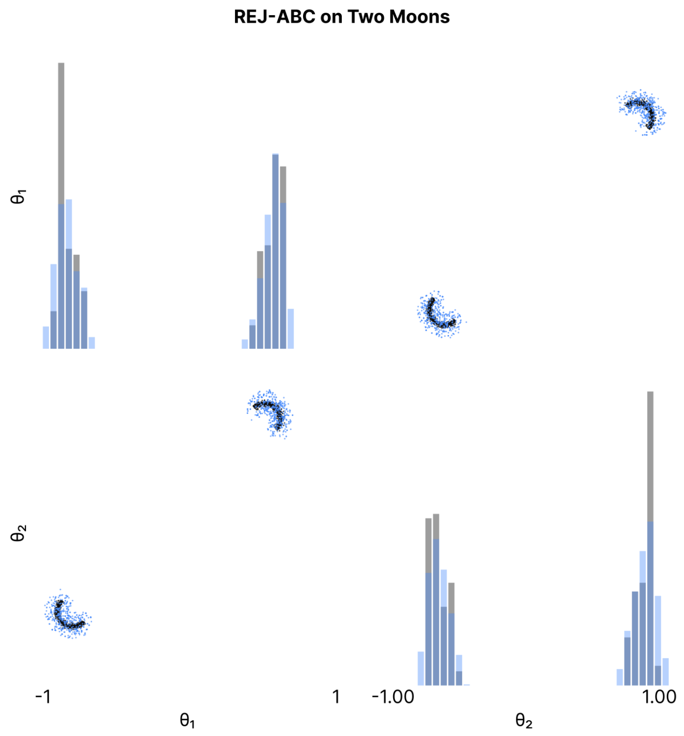
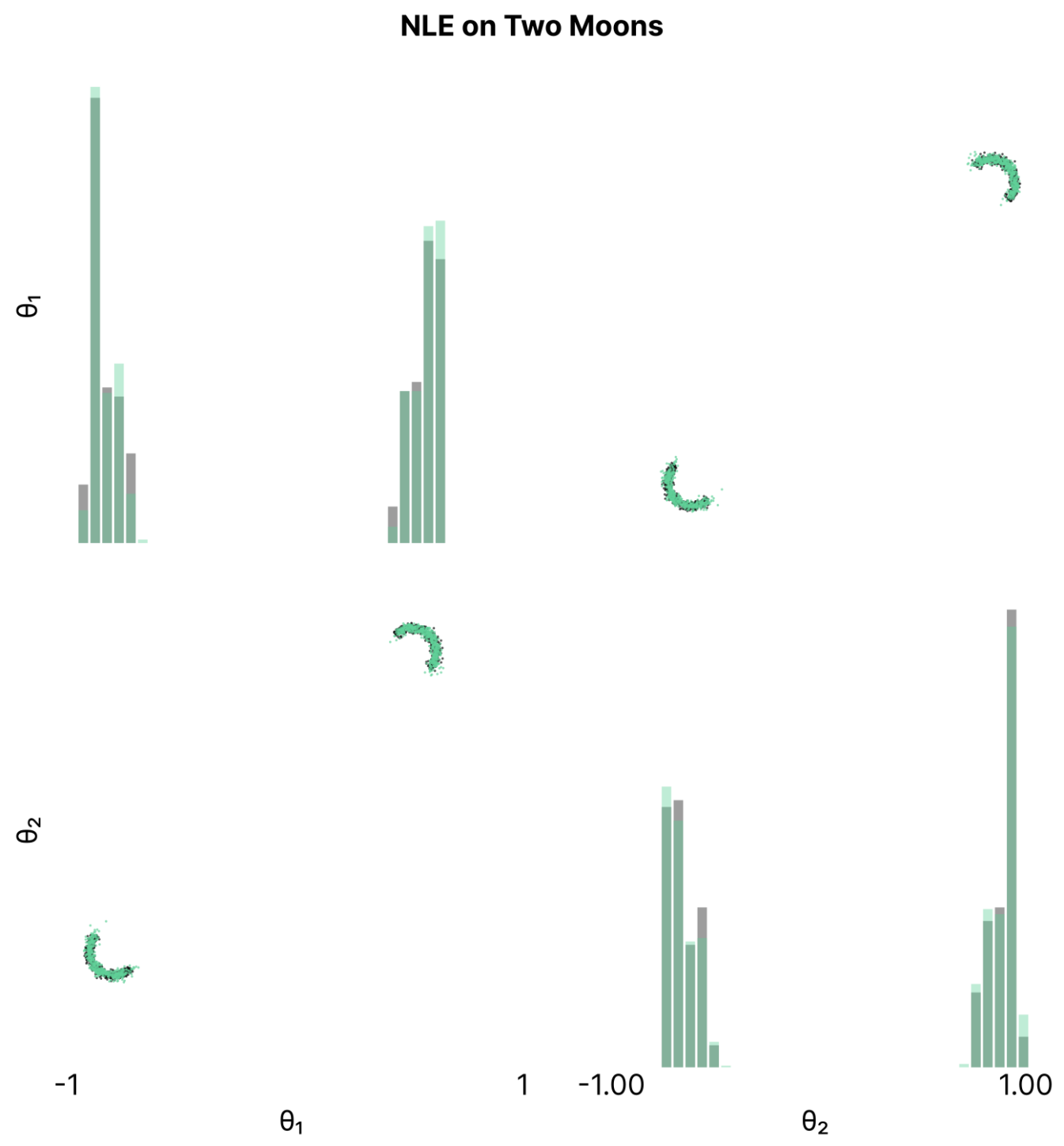
Figure 4: MMD on Two Moons. When using MMD with the median heuristic (as commonly done, including in SBI papers), MMD is slightly lower for the posterior obtained by REJ-ABC (left, blue samples), than for SNLE samples (right, green samples): 0.00729 (REJ-ABC) versus 0.00772 (NLE). This is at odds with the visual impression of the quality of the fit (reference samples in gray) as well as C2ST results: A classifier performed near chance level (.502) for SNLE samples while being able to tell apart REJ-ABC samples from the reference with accuracy 0.794. When manually choosing a length scale on the median distance of a single crescent (i.e., 0.09 instead of 1.78), MMD results were in agreement with C2ST results: 0.00738 (REJ-ABC) versus 0.00035 (SNLE), i.e., they also suggested a better fit for SNLE. In the main paper, we prefer to report C2ST because we found it less sensitive to hyperparameters: reliance on the commonly used median heuristic can be problematic on tasks with complex posterior structure, e.g., multi-modality in Two Moons, as demonstrated here. We refer the interested reader to Liu et al. (2020) for further illustrative examples of where MMD with Gaussian kernels can have limited power. We also want to point out that new kernel-based two sample tests are being actively developed which might make them easier to use on such problems in the future.

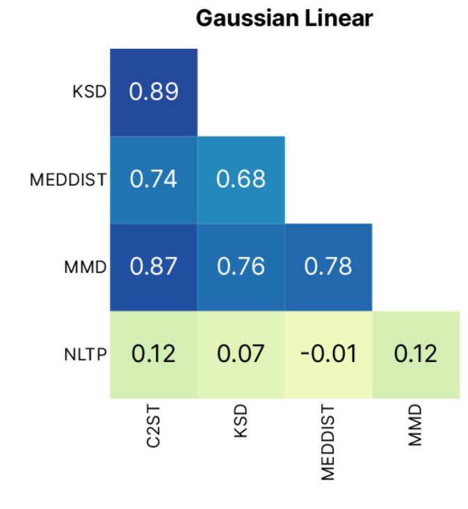
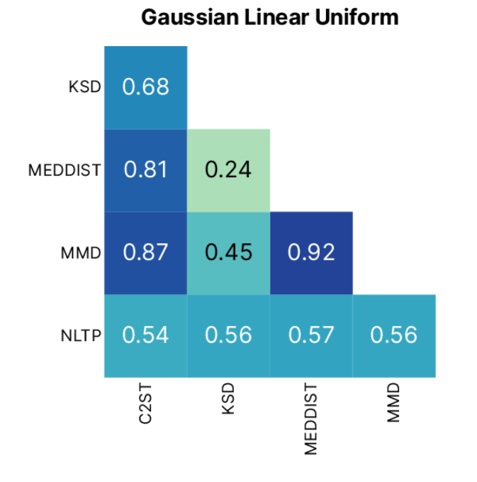
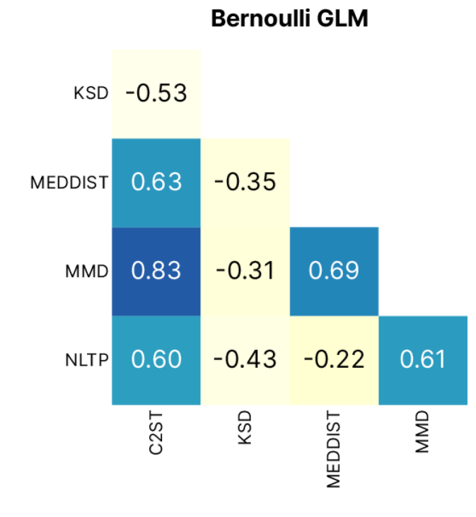
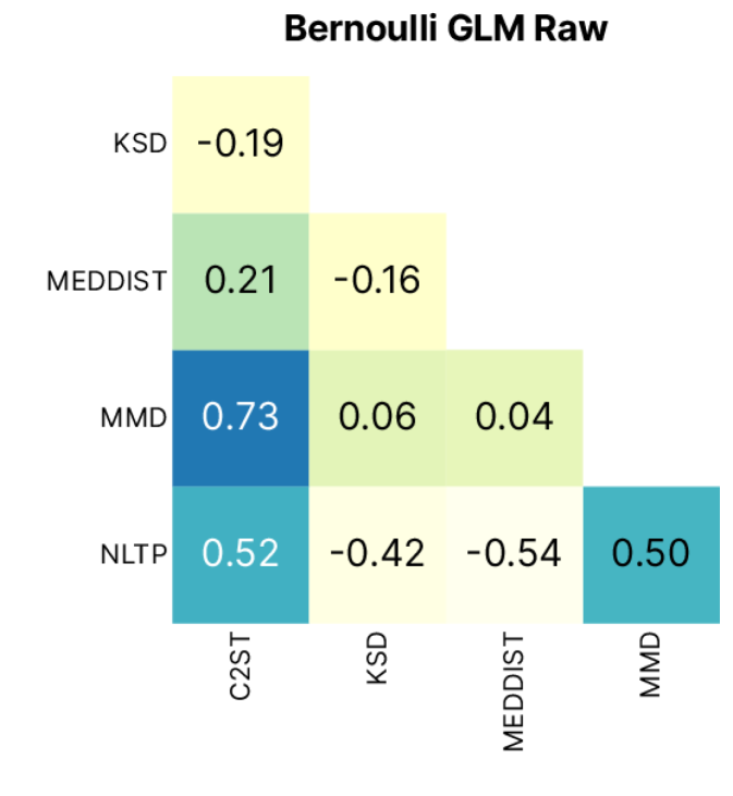
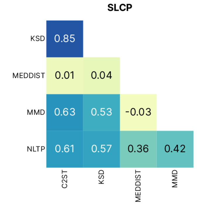
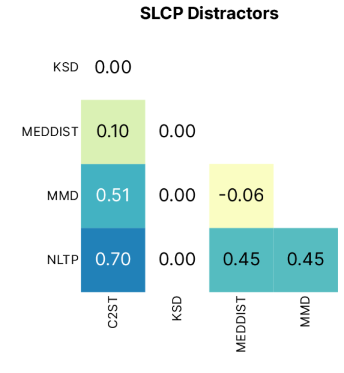
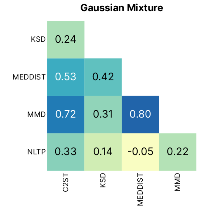
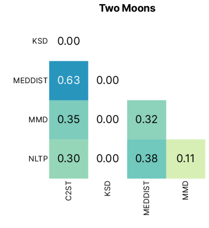
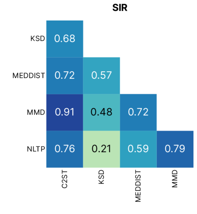
Figure 5: Correlations between metrics for all tasks. NLTP is the negative log probability of true parameters. Note that calculation of KSD was numerically unstable when calculating gradients for SLCP Distractors and Two Moons, resulting in correlation of zero for these tasks.

Appendix H Hyperparameter Choices

In this section, we address two central questions for any benchmark: (1) how hyperparameters are chosen and (2) how sensitive results are to the respective choices.

Rather than tuning hyperparameters on a per-task basis, we changed hyperparameters on multiple or all tasks at once and selected configurations that worked best across tasks. We wanted to avoid overfitting on individual benchmark tasks and were instead interested in settings that can generalize across multiple tasks. In practice, tuning an algorithm on a given task would typically be impossible, due to the lack of suitable metrics that can be computed without reference posteriors as well as high computational demands that SBI tasks often have.

To find good general settings, we performed more than 10 000 individual runs. We explored hyperparameter choices that have not been previously reported, and revealed substantial improvements. The benchmark offers the possibility to systematically compare different choices and design better and more robust SBI algorithms.

H.1 REJ-ABC

Classical ABC algorithms have crucial hyperparameters, most importantly, the distance metric and acceptance tolerance $\epsilon$. We used our own implementation of REJ-ABC as it is straightforward to implement (see A.1). The distance metric was fixed to be the $l_{2}$-norm for all tasks and we varied different acceptance tolerances $\epsilon$ across tasks on which REJ-ABC performed sufficiently well. Our implementation of REJ-ABC is quantile based, i.e,. we select a quantile of the samples with the smallest distance to the observed data, which implicitly defines an $\epsilon$. The 10k samples needed for the comparison to the reference posterior samples are then resampled from the selected samples. In order to check whether this resampling significantly impaired performance, we alternatively fit a KDE in order to obtain 10k samples.

Below, we show results for different schedules of quantiles for each simulation budget, e.g., a schedule of 0.1, 0.01, 0.001 corresponds to the 10, 1 and 0.1 percent quantile, or the top 100 samples for each simulation budget. Across tasks and budgets the 0.1, 0.01, 0.001 quantile schedule performed best (Fig. 6). Performance showed improvement by the KDE fit, especially on the Gaussian tasks. We therefore report the version using the top 100 samples and KDE in the main paper.

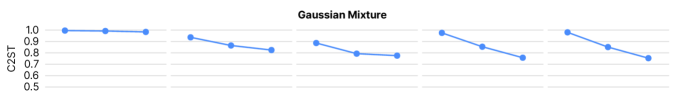
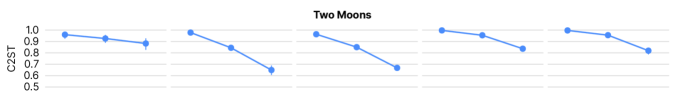
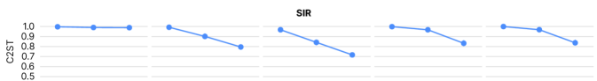
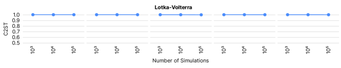
Figure 6: Hyperparameter selection for REJ-ABC. C2ST performance of different percentile schedules across simulation budgets (columns) for all tasks (rows). Top label for each plot column: number of samples retained, and optional KDE. Across tasks and budgets, the schedule of 0.1, 0.01, 0.001 percentiles, which corresponds to the top 100 samples closest to the observation, performed best. Each data point corresponds to the mean and 95% confidence interval across 10 observations.

H.2 SMC-ABC

SMC-ABC has several hyperparameters including the population size, the perturbation kernel, the epsilon schedule and the distance metric. In order to ensure that we report the best possible SMC-ABC results for a fair comparison, we sweeped over three hyperparameters that are especially critical: the population size, the quantile used to select the epsilon from the distances of the particles of the previous population, and the scaling factor of the covariance of the Gaussian perturbation kernel. The remaining hyperparameters were fixed to values common in the literature: Gaussian perturbation kernel and $l2$-norm distance metric.

Additionally, we compared our implementation against one from the popular pyABC toolbox (Klinger et al., 2018) to which we refer as versions A and B respectively. We sweeped over these hyperparameters and optionally added a post-hoc KDE fit for drawing the samples needed for two-sample based performance metrics.

Overall, the parameter setting with a population size of 100, a kernel covariance scale of 0.5, and an epsilon quantile 0.2 performed best. Although the results of the two different implementations were qualitatively very similar (compare Fig. 7 and Fig. 8, respectively), version A was slightly better on the Gaussian tasks. Although we tried to match the implementations and the exact settings, there are small differences between the two, which might explain the difference in the results: Implementation B constructs the Gaussian perturbation kernel using kernel density estimation on the weighted samples of the previous population, whereas A constructs it using the mean and covariance estimated from samples from the previous population. The latter could be advantageous in case of a Gaussian-like (high-dimensional) posterior (Gaussian Mixture and Gaussian linear task) and disadvantageous in a non-Gaussian-like posteriors (e.g., Two Moons). We decided to report results for SMC-ABC in the main paper using implementation A (ours) with population size 100 for simulation budgets 1k and 10k, and population size 1000 for simulation budget 100k, a kernel covariance scale of 0.5, and epsilon quantile 0.2. This choice of kernel covariance scale is different from recommendations in the literature (Sisson et al., 2007; Beaumont et al., 2009). We only found very small performance differences for different scales and note that our choice is in line with the recommendation of the pyABC toolbox (pyABC API Documentation, 2020), i.e., using a scale between 0 and 1. Performance showed improvement by the KDE fit, especially on the Gaussian tasks. We therefore report the version with KDE in the main paper.

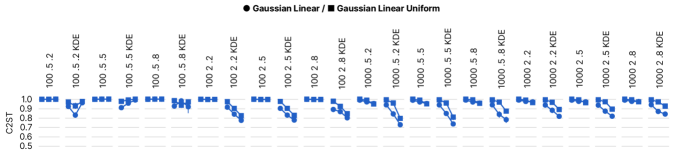
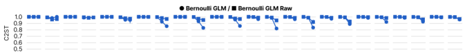
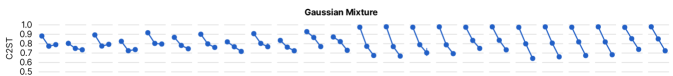
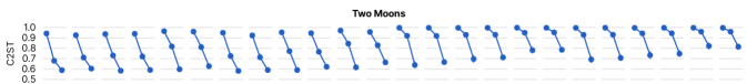
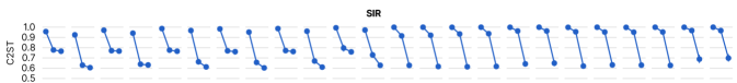
Figure 7: Hyperparameter selection for SMC-ABC with our implementation. Top label for each plot column: population size, kernel covariance scale, epsilon quantile/epsilon-decay parameter, and optional KDE. Each data point corresponds to the mean and 95% confidence interval across 10 observations.

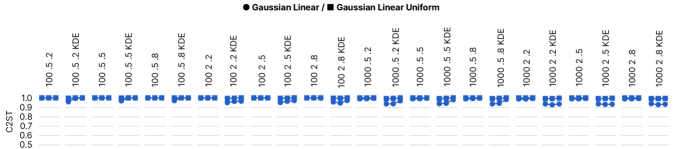
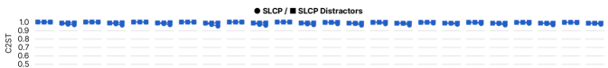
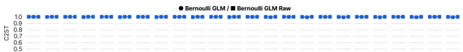
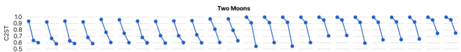
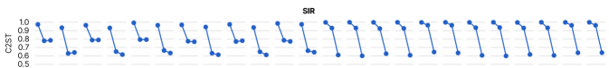
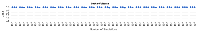
Figure 8: Hyperparameter selection for SMC-ABC. with pyABC implementation. Top label for each plot column: population size, kernel covariance scale, epsilon quantile/epsilon-decay parameter, and optional KDE. Each data point corresponds to the mean and 95% confidence interval across 10 observations.

H.3 MCMC for (S)NLE and (S)NRE

(S)NLE and (S)NRE both rely on MCMC sampling, which has several hyperparameters. In line with Papamakarios et al. (2019b) and Durkan et al. (2020), we used Slice Sampling (Neal, 2003). However, we modified the MCMC schemes used in these papers and obtained significant improvements in performance and speed.

Number of chains and initialization. While Papamakarios et al. (2019b); Durkan et al. (2020) used a single chain with axis-aligned updates, we found that on tasks with multi-modal posteriors, it can be essential to run multiple MCMC chains in order to sample all modes. Performance on Two Moons, for example, was poor with a single chain, since usually only one of the crescent shapes was sampled. Rather than initialising chains by drawing initial locations from the prior, we found the resampling scheme as described in A.3 to work better for initialisation, and used 100 chains instead of a single one.

Transformation of variables. When implementing MCMC, it is common advice to transform problems to have unbounded support (Hogg and Foreman-Mackey, 2018), although this has not been discussed in SBI papers or implemented in accompanying code. We found that without this transformation, MCMC sampling could get stuck in endless loops, e.g., on the Lotka-Volterra task. Apart from the transformation to unbounded space, we found z-scoring of parameters and data to be crucial for some tasks.

Vectorization of MCMC sampling. We reimplemented Slice Sampling so that all chains could perform likelihood evaluations in parallel. Evaluating likelihoods, e.g., in the case of (S)NLE, requires passes through a flow-based density estimator, which is significantly faster when batched. This allowed us to sample all chains in parallel rather than sequentially and yielded huge speed-ups: For example, SNLE on Gaussian Linear took more than 36 hours on average for 100k simulations without vectorization, and less than 2 hours with vectorization.

H.4 Density estimator for (S)NLE

Approaches based on neural networks (NN) tend to have many hyperparameters, including the concrete type of NN architecture and hyperparameters for training. We strove to keep our choices close to Durkan et al. (2020), which are the defaults in the toolbox we used (sbi, Tejero-Cantero et al., 2020).

While Papamakarios et al. (2019b); Durkan et al. (2020) used Masked Autoregressive Flows (MAFs, Papamakarios et al., 2017) for density estimation, we explored how results change when using Neural Spline Flows (NSFs, Durkan et al., 2019) for density estimation. These results are shown in Fig. 9.

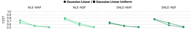
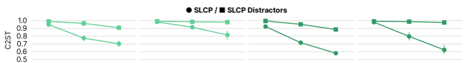
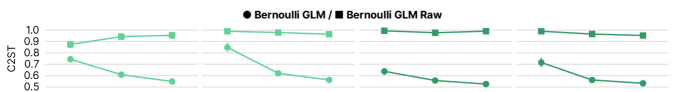
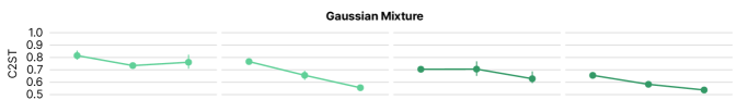
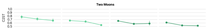
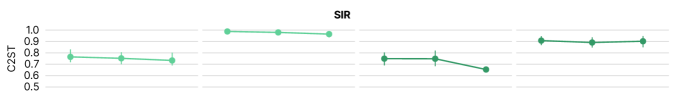
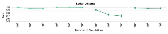
Figure 9: Density estimator selection for (S)NLE. Performance of (S)NLE in terms of C2ST across tasks using MAFs or NSFs for density estimation. Considering all tasks, NSFs generally performed worse, e.g., using NSFs significantly reduced performance on SIR and Lotka-Volterra, indicating that the added flexibility of NSFs was not needed for (S)NLE. We thus reported performance using MAFs in the main paper. Each data point corresponds to the mean and 95% confidence interval across 10 observations.

H.5 Density estimator for (S)NPE

We performed the analogous experiments for (S)NPE as for (S)NLE: Here, we found NSFs to increase performance relative to MAFs (Fig. 10). When directly estimating the posterior distribution, especially on tasks with complex multi-modal structure like Two Moons or SLCP, the additional flexibility offered by NSFs improved performance. With NSFs, artifacts from density transformation that were visible e.g. in Two Moons posteriors, vanished. To our knowledge, results on (S)NPE with NSFs have not been previously published.

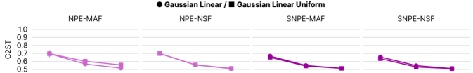
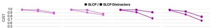
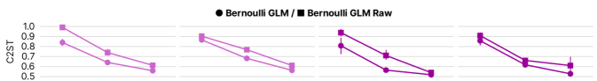
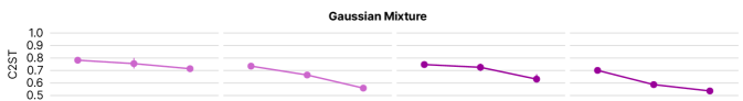
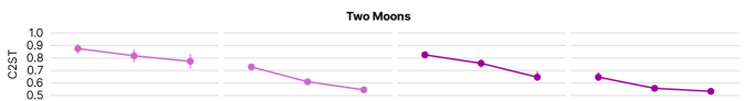
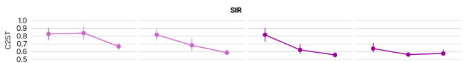
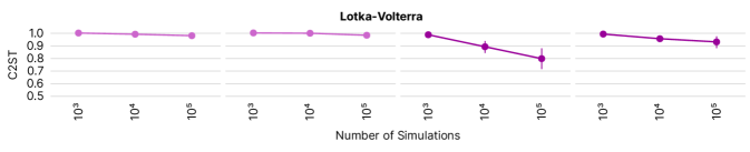
Figure 10: Density estimator selection for (S)NPE. Performance of (S)NPE in terms of C2ST across tasks using MAFs or NSFs for density estimation. Considering all tasks, NSFs generally performed better, especially on Gaussian Mixture, Two Moons, and SIR. We thus reported performance using NSFs in the main paper. Each data point corresponds to the mean and 95% confidence interval across 10 observations.

H.6 Classifier choice for (S)NRE

For (S)NRE, we compared two different choices of classifier architectures: an MLP and a ResNet architecture, as described in A.7. While results were similar for most tasks (Fig. 11), we decided to use the ResNet architecture in the main paper due to the better performance on Two Moons and SIR for low to medium simulation budgets.

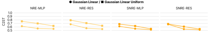
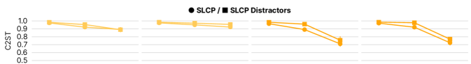
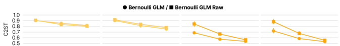
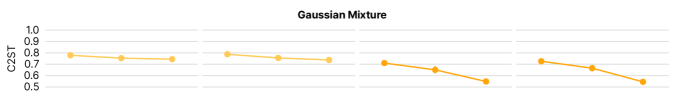
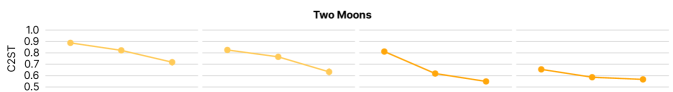
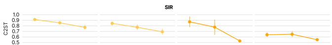
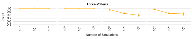
Figure 11: Classifier architecture for (S)NRE. Performance of (S)NRE in terms of C2ST across tasks using MLPs or ResNets for classification. Considering all tasks, ResNets generally performed better, especially on Two Moons and SIR. We thus reported performance using ResNets in the main paper. Each data point corresponds to the mean and 95% confidence interval across 10 observations.

Appendix M Metrics

M.1 Negative log probability of $\boldsymbol{\mathbf{\theta}}_{o}$ (NLTP)

In simulation-based inference, the average negative log likelihood of true parameters $-\mathbb{E}[\log q(\boldsymbol{\mathbf{\theta}}_{o}|\boldsymbol{\mathbf{x}}_{o})]$ (NLTP) is commonly reported as a performance metric in the literature (Papamakarios and Murray, 2016; Durkan et al., 2018; Papamakarios et al., 2019b; Greenberg et al., 2019; Hermans et al., 2020; Durkan et al., 2020). An attractive property of this metric is that the access to the ground-truth posterior is not required.

It is important to point out, however, that calculating this metric on a single or small number of pairs $(\boldsymbol{\mathbf{\theta}}_{o},\boldsymbol{\mathbf{x}}_{o})$ is problematic. To illustrate the issue, consider the following example (as discussed in Talts et al. (2018)): Consider $\theta\sim\mathcal{N}(0,1^{2}),x|\theta\sim\mathcal{N}(\theta,{1}^{2})$, and a single pair $(\boldsymbol{\mathbf{\theta}}_{o},\boldsymbol{\mathbf{x}}_{o})$ with $\theta_{o}=0$ and an implausible (but possible) $x_{o}=2.1$. In this case, the true posterior is $\mathcal{N}(\theta|1.05,0.5^{2})$ under which the $\theta_{o}$ has low probability since it is more than two standard deviations away from the posterior mean. If an algorithm fitted a wrong posterior, e.g., by overestimating the standard deviation as 1 instead of 0.5, the probability of $\theta_{o}$ under the estimated posterior would be higher than under the true posterior.

Therefore, a large number of pairs $(\boldsymbol{\mathbf{\theta}}_{o},\boldsymbol{\mathbf{x}}_{o})$ should be used. Indeed, in the limit of infinite number of pairs $(\boldsymbol{\mathbf{\theta}}_{o},\boldsymbol{\mathbf{x}}_{o})$, the metric converges to a $D_{\text{KL}}$:

$$\mathbb{E}_{\boldsymbol{\mathbf{\theta}}_{o}\sim p(\boldsymbol{\mathbf{\theta}})}\mathbb{E}_{\boldsymbol{\mathbf{x}}_{o}\sim p(\boldsymbol{\mathbf{x}}|\boldsymbol{\mathbf{\theta}}_{o})}\big{[}-\log q(\boldsymbol{\mathbf{\theta}}_{o}|\boldsymbol{\mathbf{x}}_{o})\big{]}$$

$$= \mathbb{E}_{\boldsymbol{\mathbf{x}}_{o}\sim p(\boldsymbol{\mathbf{x}}),\boldsymbol{\mathbf{\theta}}_{o}\sim p(\boldsymbol{\mathbf{\theta}}|\boldsymbol{\mathbf{x}}_{o})}\big{[}-\log q(\boldsymbol{\mathbf{\theta}}_{o}|\boldsymbol{\mathbf{x}}_{o})\big{]}$$

$$= \mathbb{E}_{\boldsymbol{\mathbf{x}}_{o}\sim p(\boldsymbol{\mathbf{x}}),\boldsymbol{\mathbf{\theta}}_{o}\sim p(\boldsymbol{\mathbf{\theta}}|\boldsymbol{\mathbf{x}}_{o})}\big{[}-\log q(\boldsymbol{\mathbf{\theta}}_{o}|\boldsymbol{\mathbf{x}}_{o})+\log p(\boldsymbol{\mathbf{\theta}}_{o}|\boldsymbol{\mathbf{x}}_{o})\big{]}-\mathbb{E}_{\boldsymbol{\mathbf{x}}_{o}\sim p(\boldsymbol{\mathbf{x}}),\boldsymbol{\mathbf{\theta}}_{o}\sim p(\boldsymbol{\mathbf{\theta}}|\boldsymbol{\mathbf{x}}_{o})}\big{[}\log p(\boldsymbol{\mathbf{\theta}}_{o}|\boldsymbol{\mathbf{x}}_{o})\big{]}$$

$$= \mathbb{E}_{\boldsymbol{\mathbf{x}}_{o}\sim p(\boldsymbol{\mathbf{x}})}D_{\text{KL}}(p(\boldsymbol{\mathbf{\theta}}|\boldsymbol{\mathbf{x}}_{o})||q(\boldsymbol{\mathbf{\theta}}|\boldsymbol{\mathbf{x}}_{o}))+\mathbb{E}_{\boldsymbol{\mathbf{x}}_{o}\sim p(\boldsymbol{\mathbf{x}})}\mathbb{H}(p(\boldsymbol{\mathbf{\theta}}|\boldsymbol{\mathbf{x}}_{o}))$$

The first term in the final equation is the average $D_{\text{KL}}$ between true and approximate posteriors over all observations $\boldsymbol{\mathbf{x}}_{o}$ that can be generated when sampling parameters $\boldsymbol{\mathbf{\theta}}_{o}$ from the prior. The second term, the entropy term, would be the same for all algorithms compared.

In the context of this benchmark, we decided against using the probability of $\boldsymbol{\mathbf{\theta}}_{o}$ as a metric: For all algorithms that are not amortized (all but one), evaluating posteriors at different $\boldsymbol{\mathbf{x}}_{o}$ would require rerunning inference. As the computational requirements for running the benchmark at 10 observations per task are already high, running tasks for hundreds of observations would become prohibitively expensive.

M.2 Simulation-based calibration (SBC)

In simulation-based calibration (SBC), samples $\boldsymbol{\mathbf{\theta}}^{\prime}$ are drawn from the data-averaged posterior, i.e., the posterior obtained by running inference for many observations. When the posterior approximation is exact, $\boldsymbol{\mathbf{\theta}}^{\prime}$ is distributed according to the prior (Talts et al., 2018).

Let us briefly illustrate this: In SBC, we draw $\boldsymbol{\mathbf{\theta}}\sim p(\boldsymbol{\mathbf{\theta}}),\boldsymbol{\mathbf{x}}\sim p(\boldsymbol{\mathbf{x}}|\boldsymbol{\mathbf{\theta}}),\boldsymbol{\mathbf{\theta}}^{\prime}\sim q(\boldsymbol{\mathbf{\theta}}^{\prime}|\boldsymbol{\mathbf{x}})$, which implies a joint distribution $\pi(\boldsymbol{\mathbf{\theta}},\boldsymbol{\mathbf{x}},\boldsymbol{\mathbf{\theta}}^{\prime})=p(\boldsymbol{\mathbf{\theta}})p(\boldsymbol{\mathbf{x}}|\boldsymbol{\mathbf{\theta}})q(\boldsymbol{\mathbf{\theta}}^{\prime}|\boldsymbol{\mathbf{x}})$. The marginal $\pi(\boldsymbol{\mathbf{\theta}}^{\prime})$ is then:

$$\pi(\boldsymbol{\mathbf{\theta}}^{\prime})=\int\int p(\boldsymbol{\mathbf{\theta}})p(\boldsymbol{\mathbf{x}}|\boldsymbol{\mathbf{\theta}})q(\boldsymbol{\mathbf{\theta}}^{\prime}|\boldsymbol{\mathbf{x}})\operatorname{d}\!{\boldsymbol{\mathbf{x}}}\operatorname{d}\!{\boldsymbol{\mathbf{\theta}}}=\int\int p(\boldsymbol{\mathbf{\theta}},\boldsymbol{\mathbf{x}})q(\boldsymbol{\mathbf{\theta}}^{\prime}|\boldsymbol{\mathbf{x}})\operatorname{d}\!{\boldsymbol{\mathbf{x}}}\operatorname{d}\!{\boldsymbol{\mathbf{\theta}}}=\int p(\boldsymbol{\mathbf{x}})\ q(\boldsymbol{\mathbf{\theta}}^{\prime}|\boldsymbol{\mathbf{x}})\operatorname{d}\!{\boldsymbol{\mathbf{x}}}.$$

If the approximate posterior is the true posterior, the marginal on $\boldsymbol{\mathbf{\theta}}^{\prime}$ is equal to the prior: If $q(\boldsymbol{\mathbf{\theta}}^{\prime}|\boldsymbol{\mathbf{x}})=p(\boldsymbol{\mathbf{\theta}}^{\prime}|\boldsymbol{\mathbf{x}})$, then $\pi(\boldsymbol{\mathbf{\theta}}^{\prime})=\int p(\boldsymbol{\mathbf{x}},\boldsymbol{\mathbf{\theta}}^{\prime})\operatorname{d}\!{\boldsymbol{\mathbf{x}}}=p(\boldsymbol{\mathbf{\theta}}^{\prime})$, i.e., one can set up a consistency test that is based on the distribution of $\boldsymbol{\mathbf{\theta}}^{\prime}$ samples. Talts et al. (2018) do this by using frequentist tests per dimension.

Note that SBC as described above is merely a consistency check. For example, if the approximate posterior were the prior, a calibration test as described above would not be able to detect this. This is a realistic failure mode in simulation-based inference. It could happen with rejection ABC in the limit $\epsilon\rightarrow\infty$, or when learned summary statistics have no information about $\boldsymbol{\mathbf{\theta}}$. One way around this is issue is proposed in Prangle et al. (2014a), who propose to restrict observations to a subset of all possible $\mathcal{X}$.

SBC is similar to the average negative log likelihood of true parameters described above, in that inference needs to be carried out for many observations generated by sampling from the prior. Running inference for hundreds of observations would become prohibitively expensive in terms of compute for most algorithms, which is why we do not rely on SBC in the benchmark.

M.3 Median distance (MEDDIST)

Posterior predictive checks (PPCs) use the posterior predictive distribution to predict new data, $\boldsymbol{\mathbf{x}}^{\prime}\sim p(\boldsymbol{\mathbf{x}}^{\prime}|\boldsymbol{\mathbf{x}}_{o})=\int p(\boldsymbol{\mathbf{x}}^{\prime}|\boldsymbol{\mathbf{\theta}})q(\boldsymbol{\mathbf{\theta}}|\boldsymbol{\mathbf{x}}_{o})\operatorname{d}\!{\boldsymbol{\mathbf{\theta}}}$. The observed data $\boldsymbol{\mathbf{x}}_{o}$ should look plausible under the posterior predictive distribution (Gelman et al. (2004), chapter 6). A particular PPC, used for example in Papamakarios et al. (2019b); Greenberg et al. (2019); Durkan et al. (2020), is to assess the median L2 distance between $N^{\prime}$ posterior predictive samples $\boldsymbol{\mathbf{x}}^{\prime}$ and $\boldsymbol{\mathbf{x}}_{o}$. The median is used since the mean would be more sensitive to outliers.

In the benchmark, we refer to this metric as median distance (MEDDIST) and drew $N^{\prime}=10000$ samples from each posterior predictive distribution to compute it. In contrast with other metrics considered here, the median distance is computed in the space of data $\boldsymbol{\mathbf{x}}$ and requires additional simulations (which could be expensive, depending on the simulator). The median distance should be considered a mere check rather than a metric and it does not necessarily test the structure of the estimated posterior.

M.4 Maximum Mean Discrepancy (MMD)

Maximum Mean Discrepancy (MMD) is an Integral Probability Metric (IPM). Linear and quadratic time estimates for using MMD as a two-sample test were derived in Gretton et al. (2012). MMD has been commonly used in the SBI literature with Gaussian kernels (Papamakarios et al., 2019b; Greenberg et al., 2019; Hermans et al., 2020), setting a single length-scale hyperparameter by using a median heuristic (Ramdas et al., 2015). We follow the same procedure, i.e., use Gaussian kernels with length-scale determined by the median heuristic on reference samples. MMDs are calculated using 10k samples from reference and approximate posteriors.

If simple kernels are used to compare distributions with complex, multimodal structure, distinct distributions can be mapped to nearby mean embeddings, resulting in low test power. On SLCP and Two Moons, for example, we found a translation-invariant kernel to be limiting, since it cannot adapt to the local structure (see Suppl. Fig. 4). This is reflected in the low correlation of MMD and C2ST (Suppl. Fig. 5). We emphasize that these issues are strictly related to simple kernels with hyperparameters commonly used in the literature. Posteriors of the Two Moons task have a structure similar to the blobs example of Liu et al. (2020), who argue for using learned kernels to overcome the aforementioned problem.

M.5 Classifier-based tests (C2ST)

In classifier-based testing, a classifier is trained to distinguish samples of the true posterior $p(\boldsymbol{\mathbf{\theta}}|\boldsymbol{\mathbf{x}}_{o})$ from samples of the estimated posterior $q(\boldsymbol{\mathbf{\theta}}|\boldsymbol{\mathbf{x}}_{o})$. If the samples are indistinguishable, the classification performance should be at chance level, 0.5. Practical use and properties of classifier-based 2-sample testing (C2ST) are discussed in Lopez-Paz and Oquab (2017) (see Gutmann et al., 2018; Dalmasso et al., 2020, for examples in the context of SBI).

To compute C2ST, we trained a two-layer neural network with 10 times as many ReLU units as the dimensionality of parameters, and optimize with Adam (Kingma and Ba, 2015). Classifiers were trained on 10k z-scored samples from reference and approximate posterior each. Classification accuracy was reported using 5-fold cross-validation.

M.6 Kernelized Stein Discrepancy (KSD)

Kernelized Stein Discrepancy (KSD) is a 1-sample goodness-of-fit test proposed independently by Chwialkowski et al. (2016) and Liu et al. (2016). KSD tests samples from algorithms against the gradient of unnormalized true posterior density, $\nabla_{\boldsymbol{\mathbf{\theta}}}\ \tilde{p}(\boldsymbol{\mathbf{\theta}}|\boldsymbol{\mathbf{x}}_{o})$. We used KSD with Gaussian kernels, setting the length-scale through the median heuristic, and 10k samples from each algorithm.

Appendix R Runtimes

In applications of SBI, simulations are commonly assumed to be the dominant cost. In order to make the benchmark feasible at this scale, we focused on simple simulators and optimized runtimes, e.g. we developed a new package bridging DifferentialEquations.jl (Rackauckas and Nie, 2017; Bezanson et al., 2017) and PyTorch (Paszke et al., 2019) so that generating simulations for all implemented tasks is extremely fast. This differs from many cases in practice, where the runtime costs for an algorithm are often negligible compared to the cost of simulations. Having said that, algorithms show significant differences in runtime costs, which we measured and report here.

We recorded runtimes for all algorithms on all tasks. In principle, runtimes could be reduced by employing multi-CPU architectures, however, we decided for the single CPU setup to accurately compare runtimes across all algorithms and tasks. We did not employ GPUs for training neural-networks (NN). This is because the type of NNs used in the algorithms currently in the benchmark do not benefit much from GPU versus CPU training (e.g., no CNN architecture, rather shallow and narrow networks). In fact, running SNPE on SLCP using a GeForce GTX 1080 showed slightly longer runtimes than on CPU, due to the added overhead resulting from copying data back and forth to the device. Therefore, it was more economical and comparable to run the benchmark on CPUs.

All neural network-based algorithms were run on single 3.6 GHz CPU cores of AWS C5-instances. ABC algorithms were run on single CPU cores of an internal cluster with 2.4 GHz CPUs. We observed a difference in runtimes of less than 100ms when running ABC algorithms on the same hardware as used for neural network-based algorithms.

Figure 12 shows the recorded runtimes in minutes. We observed short runtimes for REJ-ABC and SMC-ABC, as these do not require NN training or MCMC. The sequential versions of all three NN-based algorithms yielded longer runtimes than the non-sequential versions because these involve 10 rounds of NN training. Among the sequential algorithms, SNPE showed the longest runtimes. Runtimes with MAFs instead of NSFs tend to be faster, e.g. the difference between MAFs and NSFs using SNPE on SLCP at 100k simulations was about 50 minutes on average. We also emphasize that the speed of (S)NLE reported here was only obtained after vectorizing MCMC sampling. Without vectorization, runtime on the Gaussian Linear for SNLE was more than 36 hours instead of less than 2 hours (see Appendix H).

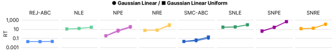
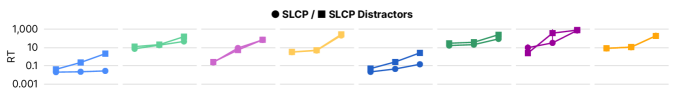
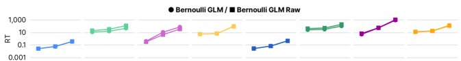
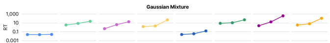
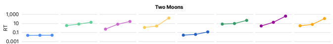
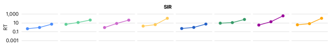
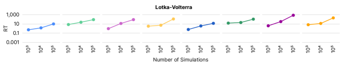
Figure 12: Runtime on benchmark tasks. Runtime of REJ-ABC, SMC-ABC, NLE, SNLE, NPE, SNPE, NRE, SNRE in minutes, for 10 observations each, means and 95% confidence intervals. Each run was allocated a single CPU core, see Appendix R for details.

Appendix T Tasks

T.1 Gaussian Linear

Inference of the mean of a 10-d Gaussian model, in which the covariance is fixed. The (conjugate) prior is Gaussian:

Prior	$\mathcal{N}(\boldsymbol{\mathbf{0}},0.1\odot\boldsymbol{\mathbf{I}})$
Simulator	$\boldsymbol{\mathbf{x}}|\boldsymbol{\mathbf{\theta}}\sim\mathcal{N}(\boldsymbol{\mathbf{x}}|\boldsymbol{\mathbf{m}}_{\boldsymbol{\mathbf{\theta}}}=\boldsymbol{\mathbf{\theta}},\boldsymbol{\mathbf{S}}=0.1\odot\boldsymbol{\mathbf{I}})$
Dimensionality	$\boldsymbol{\mathbf{\theta}}\in\mathbb{R}^{10},\boldsymbol{\mathbf{x}}\in\mathbb{R}^{10}$

T.2 Gaussian Linear Uniform

Inference of the mean of a 10-d Gaussian model, in which the covariance is fixed. The prior is uniform:

Prior	$\mathcal{U}(-\boldsymbol{\mathbf{1}},\boldsymbol{\mathbf{1}})$
Simulator	$\boldsymbol{\mathbf{x}}|\boldsymbol{\mathbf{\theta}}\sim\mathcal{N}(\boldsymbol{\mathbf{x}}|\boldsymbol{\mathbf{m}}_{\boldsymbol{\mathbf{\theta}}}=\boldsymbol{\mathbf{\theta}},\boldsymbol{\mathbf{S}}=0.1\odot\boldsymbol{\mathbf{I}})$
Dimensionality	$\boldsymbol{\mathbf{\theta}}\in\mathbb{R}^{10},\boldsymbol{\mathbf{x}}\in\mathbb{R}^{10}$

T.3 SLCP

A challenging inference task designed to have a simple likelihood and a complex posterior. The prior is uniform over five parameters $\boldsymbol{\mathbf{\theta}}$ and the data are a set of four two-dimensional points sampled from a Gaussian likelihood whose mean and variance are nonlinear functions of $\boldsymbol{\mathbf{\theta}}$:

Prior	$\mathcal{U}(-\boldsymbol{\mathbf{3}},\boldsymbol{\mathbf{3}})$
Simulator	$\boldsymbol{\mathbf{x}}|\boldsymbol{\mathbf{\theta}}=(\boldsymbol{\mathbf{x}}_{1},\ldots,\boldsymbol{\mathbf{x}}_{4})$, $\boldsymbol{\mathbf{x}}_{i}\sim\mathcal{N}(\boldsymbol{\mathbf{m}}_{\boldsymbol{\mathbf{\theta}}},\boldsymbol{\mathbf{S}}_{\boldsymbol{\mathbf{\theta}}})$, where $\boldsymbol{\mathbf{m}}_{\boldsymbol{\mathbf{\theta}}}=\begin{bmatrix}{\theta_{1}}\\ {\theta_{2}}\end{bmatrix}$, $\boldsymbol{\mathbf{S}}_{\boldsymbol{\mathbf{\theta}}}=\begin{bmatrix}{s_{1}^{2}}&{\rho s_{1}s_{2}}\\ {\rho s_{1}s_{2}}&{s_{2}^{2}}\end{bmatrix}$, $s_{1}=\theta_{3}^{2},s_{2}=\theta_{4}^{2},\rho=\tanh\theta_{5}$
Dimensionality	$\boldsymbol{\mathbf{\theta}}\in\mathbb{R}^{5},\boldsymbol{\mathbf{x}}\in\mathbb{R}^{8}$
References	Papamakarios et al. (2019b); Greenberg et al. (2019); Hermans et al. (2020) Durkan et al. (2020)

T.4 SLCP with Distractors

This task is similar to T.3, with the difference that we add uninformative dimensions (distractors) to the observation:

Prior	$\mathcal{U}(-\boldsymbol{\mathbf{3}},\boldsymbol{\mathbf{3}})$
Simulator	$\boldsymbol{\mathbf{x}}|\boldsymbol{\mathbf{\theta}}=(\boldsymbol{\mathbf{x}}_{1},\ldots,\boldsymbol{\mathbf{x}}_{100})$, $\boldsymbol{\mathbf{x}}=p(\boldsymbol{\mathbf{y}})$, where $p$ re-orders the dimensions of $\boldsymbol{\mathbf{y}}$ with a fixed random permutation, $\boldsymbol{\mathbf{y}}_{[1:8]}\sim\mathcal{N}(\boldsymbol{\mathbf{m}}_{\boldsymbol{\mathbf{\theta}}},\boldsymbol{\mathbf{S}}_{\boldsymbol{\mathbf{\theta}}})$, $\boldsymbol{\mathbf{y}}_{[9:100]}\sim\frac{1}{20}\sum_{i=1}^{20}t_{2}(\boldsymbol{\mathbf{\mu}}^{i},\boldsymbol{\mathbf{\Sigma}}^{i})$ where $\boldsymbol{\mathbf{m}}_{\boldsymbol{\mathbf{\theta}}}=\begin{bmatrix}{\theta_{1}}\\ {\theta_{2}}\end{bmatrix}$, $\boldsymbol{\mathbf{S}}_{\boldsymbol{\mathbf{\theta}}}=\begin{bmatrix}{s_{1}^{2}}&{\rho s_{1}s_{2}}\\ {\rho s_{1}s_{2}}&{s_{2}^{2}}\end{bmatrix}$, $s_{1}=\theta_{3}^{2},s_{2}=\theta_{4}^{2},\rho=\tanh\theta_{5}$, $\boldsymbol{\mathbf{\mu}}^{i}\sim\mathcal{N}(0,15^{2}\boldsymbol{\mathbf{I}})$, $\boldsymbol{\mathbf{\Sigma}}_{j,k}^{i}\sim\mathcal{N}(0,9)$, for $j>k$, $\boldsymbol{\mathbf{\Sigma}}_{j,j}^{i}=3e^{a}$, where $a\sim\mathcal{N}(0,1)$, $\boldsymbol{\mathbf{\Sigma}}_{j,k}^{i}=0$ otherwise
Dimensionality	$\boldsymbol{\mathbf{\theta}}\in\mathbb{R}^{5},\boldsymbol{\mathbf{x}}\in\mathbb{R}^{100}$
References	Greenberg et al. (2019)

T.5 Bernoulli GLM

Inference of a 10-parameter Generalized linear model (GLM) with Bernoulli observations, and Gaussian prior with covariance matrix which encourages smoothness by penalizing the second-order differences in the vector of parameters (De Nicolao et al., 1997). The observations are the sufficient statistics for this GLM:

Prior	$\beta\sim\mathcal{N}(0,2)$, $\boldsymbol{\mathbf{f}}\sim\mathcal{N}(\boldsymbol{\mathbf{0}},(\boldsymbol{\mathbf{F}}^{\top}\boldsymbol{\mathbf{F}})^{-1})$, $\boldsymbol{\mathbf{F}}_{i,i-2}=1$, $\boldsymbol{\mathbf{F}}_{i,i-1}=-2$, $\boldsymbol{\mathbf{F}}_{i,i}=1+\sqrt{\frac{i-1}{9}}$, $\boldsymbol{\mathbf{F}}_{i,j}=0$ otherwise, $1\leq i,j\leq 9$
Simulator	$\boldsymbol{\mathbf{x}}|\boldsymbol{\mathbf{\theta}}=(\boldsymbol{\mathbf{x}}_{1},\ldots,\boldsymbol{\mathbf{x}}_{10})$, $\boldsymbol{\mathbf{x}}_{1}=\sum_{i}^{T}z_{i}$, $\boldsymbol{\mathbf{x}}_{2:10}=\frac{1}{\boldsymbol{\mathbf{x}}_{1}}\boldsymbol{\mathbf{V}}\boldsymbol{\mathbf{z}}$, $z_{i}\sim\mathrm{Bern}(\eta(\mathbf{v}_{i}^{\top}\boldsymbol{\mathbf{f}}+\beta))$, $\eta(\cdot)=\exp(\cdot)/(1+\exp(\cdot))$, frozen input between time bins $i-8$ and $i$: $\boldsymbol{\mathbf{v}}_{i}\sim\mathcal{N}(\boldsymbol{\mathbf{0}},\boldsymbol{\mathbf{I}})$, $\boldsymbol{\mathbf{V}}=[v_{1},v_{2},\ldots,v_{T}]$
Dimensionality	$\boldsymbol{\mathbf{\theta}}\in\mathbb{R}^{10},\boldsymbol{\mathbf{x}}\in\mathbb{R}^{10}$
Fixed parameters	Duration of task $T=100$.
References	Lueckmann et al. (2017); Gonçalves et al. (2020)

T.6 Bernoulli GLM Raw

This task is similar to T.5, the sole difference being that the observations are not the sufficient statistics for the Bernoulli GLM process but the raw observations:

Prior	$\beta\sim\mathcal{N}(0,2)$, $\boldsymbol{\mathbf{f}}\sim\mathcal{N}(\boldsymbol{\mathbf{0}},(\boldsymbol{\mathbf{F}}^{\top}\boldsymbol{\mathbf{F}})^{-1})$, $\boldsymbol{\mathbf{F}}_{i,i-2}=1$, $\boldsymbol{\mathbf{F}}_{i,i-1}=-2$, $\boldsymbol{\mathbf{F}}_{i,i}=1+\sqrt{\frac{i-1}{9}}$, $\boldsymbol{\mathbf{F}}_{i,j}=0$ otherwise $1\leq i,j\leq 9$
Simulator	$\boldsymbol{\mathbf{x}}|\boldsymbol{\mathbf{\theta}}=(\boldsymbol{\mathbf{x}}_{1},\ldots,\boldsymbol{\mathbf{x}}_{100})$, $x_{i}\sim\mathrm{Bern}(\eta(\mathbf{v}_{i}^{\top}\boldsymbol{\mathbf{f}}+\beta))$, $\eta(\cdot)=\exp(\cdot)/(1+\exp(\cdot))$ frozen input between time bins $i-8$ and $i$: $\boldsymbol{\mathbf{v}}_{i}\sim\mathcal{N}(\boldsymbol{\mathbf{0}},\boldsymbol{\mathbf{I}})$,
Dimensionality	$\boldsymbol{\mathbf{\theta}}\in\mathbb{R}^{10},\boldsymbol{\mathbf{x}}\in\mathbb{R}^{100}$
Fixed parameters	Duration of task $T=100$.

T.7 Gaussian Mixture

This task is common in the ABC literature. It consists of inferring the common mean of a mixture of two two-dimensional Gaussian distributions, one with much broader covariance than the other:

Prior	$\mathcal{U}(-\boldsymbol{\mathbf{10}},\boldsymbol{\mathbf{10}})$
Simulator	$\boldsymbol{\mathbf{x}}|\boldsymbol{\mathbf{\theta}}\sim 0.5\;\mathcal{N}(\boldsymbol{\mathbf{x}}|\boldsymbol{\mathbf{m}}_{\boldsymbol{\mathbf{\theta}}}=\boldsymbol{\mathbf{\theta}},\boldsymbol{\mathbf{S}}=\boldsymbol{\mathbf{I}})+$ $0.5\;\mathcal{N}(\boldsymbol{\mathbf{x}}|\boldsymbol{\mathbf{m}}_{\boldsymbol{\mathbf{\theta}}}=\boldsymbol{\mathbf{\theta}},\boldsymbol{\mathbf{S}}=0.01\odot\boldsymbol{\mathbf{I}})$
Dimensionality	$\boldsymbol{\mathbf{\theta}}\in\mathbb{R}^{2},\boldsymbol{\mathbf{x}}\in\mathbb{R}^{2}$
References	Sisson et al. (2007); Beaumont et al. (2009); Toni et al. (2009); Simola et al. (2020)

T.8 Two Moons

A two-dimensional task with a posterior that exhibits both global (bimodality) and local (crescent shape) structure to illustrate how algorithms deal with multimodality:

Prior	$\mathcal{U}(-\boldsymbol{\mathbf{1}},\boldsymbol{\mathbf{1}})$
Simulator	$\boldsymbol{x}|\boldsymbol{\mathbf{\theta}}=\begin{bmatrix}r\cos(\alpha)+0.25\\ r\sin(\alpha)\end{bmatrix}+$ $\begin{bmatrix}{-|\theta_{1}+\theta_{2}|}/{\sqrt{2}}\\ {(-\theta_{1}+\theta_{2}})/{\sqrt{2}}\\ \end{bmatrix}$, where $\alpha\sim\mathcal{U}(-\pi/{2},\pi/2)$, $r\sim\mathcal{N}(0.1,0.01^{2})$
Dimensionality	$\boldsymbol{\mathbf{\theta}}\in\mathbb{R}^{2},\boldsymbol{\mathbf{x}}\in\mathbb{R}^{2}$
References	Greenberg et al. (2019)

T.9 SIR

The SIR model is an epidemiological model describing the dynamics of the number of individuals in three possible states: susceptible $S$, infectious $I$, and recovered or deceased $R$.

The SIR task consists in inferring the contact rate $\beta$ and the mean recovery rate $\gamma$, given a sampled number of individuals in the infectious group $I$ in 10 evenly-spaced points in time:

Prior	$\beta\sim\text{LogNormal}(\log(0.4),0.5)$ $\gamma\sim\text{LogNormal}(\log(1/8),0.2)$
Simulator	$\boldsymbol{\mathbf{x}}|\boldsymbol{\mathbf{\theta}}=(x_{1},\ldots,x_{10})$, $x_{i}\sim\mathcal{B}(1000,\frac{I}{N})$, where I is simulated from $\frac{dS}{dt}=-\beta\frac{SI}{N}$ $\frac{dI}{dt}=\beta\frac{SI}{N}-\gamma I$ $\frac{dR}{dt}=\gamma I$
Dimensionality	$\boldsymbol{\mathbf{\theta}}\in\mathbb{R}^{2},\boldsymbol{\mathbf{x}}\in\mathbb{R}^{10}$
Fixed parameters	Population size $N=1000000$ and duration of task $T=160$. Initial conditions: $(S(0),I(0),R(0))=(N-1,1,0)$
References	Kermack and McKendrick (1927)

T.10 Lotka-Volterra

This is an influential model in ecology describing the dynamics of two interacting species, most commonly prey and predator interactions. Our task consists in the inference of four parameters $\boldsymbol{\mathbf{\theta}}$ related to species interaction, given 20 summary statistics consisting of the number of individuals in both populations in 10 evenly-spaced points in time:

Prior	$\alpha\sim\text{LogNormal}(-0.125,0.5)$, $\beta\sim\text{LogNormal}(-3,0.5)$, $\gamma\sim\text{LogNormal}(-0.125,0.5)$, $\delta\sim\text{LogNormal}(-3,0.5)$
Simulator	$\boldsymbol{\mathbf{x}}|\boldsymbol{\mathbf{\theta}}=(\boldsymbol{\mathbf{x}}_{1},\ldots,\boldsymbol{\mathbf{x}}_{10})$, $\boldsymbol{\mathbf{x}}_{1,i}\sim\text{LogNormal}(\log(X),0.1)$, $\boldsymbol{\mathbf{x}}_{2,i}\sim\text{LogNormal}(\log(Y),0.1)$, $X$ and $Y$ are simulated from $\frac{dX}{dt}=\alpha X-\beta XY$ $\frac{dY}{dt}=-\gamma Y+\delta XY$
Dimensionality	$\boldsymbol{\mathbf{\theta}}\in\mathbb{R}^{4},\boldsymbol{\mathbf{x}}\in\mathbb{R}^{20}$
Fixed parameters	Duration of task $T=20$. Initial conditions: $(X(0),Y(0))=(30,1)$
References	Lotka (1920)

Appendix W Website

The companion website (sbi-benchmark.github.io) allows interactive comparisons in terms of all metrics. It also allows inspection of posterior samples of all runs, which we found insightful when choosing hyperparameters and diagnosing implementation issues. Two screenshots are provided in Fig. 13.

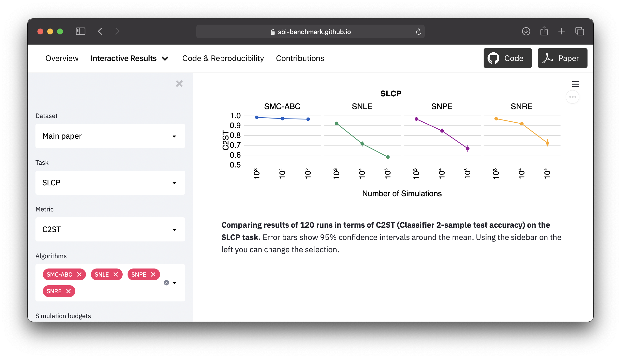
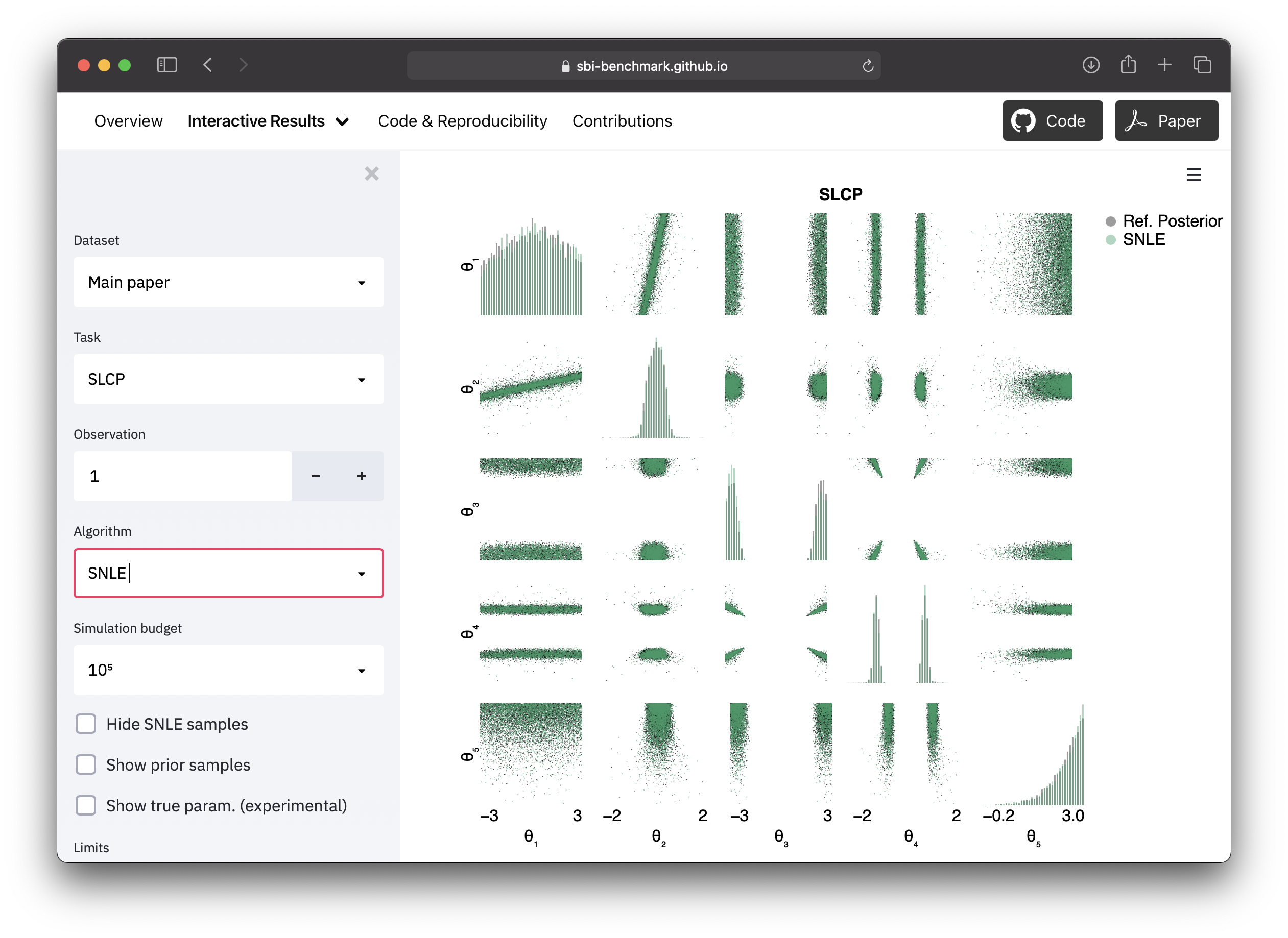
Figure 13: Screenshots from the companion website. Top: Classification accuracy (C2ST) for a subset of sequential algorithms on the SLCP task. Bottom: SNLE posterior on SLCP for $\boldsymbol{\mathbf{x}}_{o}^{(1)}$ at 100k simulations.

[section]

References

- Massive optimal data compression and density estimation for scalable, likelihood-free inference in cosmology. Monthly Notices of the Royal Astronomical Society 477 (3), pp. 2874–2885. Cited by: §1.
- Likelihood-free inference with deep gaussian processes. Deep Learning and Inverse Problems Workshop at Neural Information Processing Systems. External Links: 2006.10571 Cited by: §4.
- Etalumis: bringing probabilistic programming to scientific simulators at scale. In Proceedings of the International Conference for High Performance Computing, Networking, Storage and Analysis, pp. 1–24. Cited by: §4, Box 1.
- Adaptive approximate bayesian computation. Biometrika 96 (4), pp. 983–990. Cited by: §2.1, §2.3.
- Approximate bayesian computation in population genetics. Genetics 162 (4), pp. 2025–2035. Cited by: §2.1.
- The arcade learning environment: an evaluation platform for general agents. Journal of Artificial Intelligence Research 47, pp. 253–279. Cited by: §1.
- Julia: a fresh approach to numerical computing. SIAM review 59 (1), pp. 65–98. Cited by: §2.5, Acknowledgements.
- Pyro: deep universal probabilistic programming. Journal of Machine Learning Research 20 (1), pp. 973–978. External Links: ISSN 1532-4435 Cited by: §2.5, Acknowledgements.
- Non-linear regression models for approximate bayesian computation. Statistics and Computing 20 (1), pp. 63–73. Cited by: §2.1, §2.1, §3.
- Constraining effective field theories with machine learning. Physical Review Letters 121 (11), pp. 111801. Cited by: §1.
- Mining gold from implicit models to improve likelihood-free inference. Proceedings of the National Academy of Sciences 117 (10), pp. 5242–5249. Cited by: §1, §2.5, §4, Box 1.
- A likelihood-free inference framework for population genetic data using exchangeable neural networks. In Advances in Neural Information Processing Systems 31, pp. 8594–8605. Cited by: §1, Box 1.
- Automatic physical inference with information maximizing neural networks. Physical Review D 97 (8), pp. 083004. Cited by: Box 1.
- Neural approximate sufficient statistics for implicit models. In Proceedings of the 9th International Conference on Learning Representations, ICLR, Cited by: §4, Box 1.
- A kernel test of goodness of fit. In Proceedings of The 33rd International Conference on Machine Learning, Proceedings of Machine Learning Research, Vol. 48, pp. 2606–2615. Cited by: §2.2.
- Component-wise approximate bayesian computation via gibbs-like steps. Biometrika. External Links: Document Cited by: §4.
- Bringing abc inference to the machine learning realm: abcranger, an optimized random forests library for abc. In JOBIM 2020, Vol. 2020. Cited by: §2.5, Acknowledgements.
- The frontier of simulation-based inference. Proceedings of the National Academy of Sciences. External Links: Document Cited by: Figure 1, §1, §1, §1, §2.1, §2.5, Box 1, Box 1.
- Approximating likelihood ratios with calibrated discriminative classifiers. arXiv preprint arXiv:1506.02169. Cited by: §2.1.
- Validation of approximate likelihood and emulator models for computationally intensive simulations. In Proceedings of The 23rd International Conference on Artificial Intelligence and Statistics (AISTATS), External Links: 1905.11505 Cited by: §2.2.
- Dynamic likelihood-free inference via ratio estimation (dire). arXiv preprint arXiv:1810.09899. Cited by: §4, Box 1.
- Torch-two-sample: a pytorch library for differentiable two-sample tests. Note: Github External Links: Link Cited by: Acknowledgements.
- Approximating the likelihood in approximate bayesian computation. In Handbook of Approximate Bayesian Computation, S.A. Sisson, Y. Fan, and M. Beaumont (Eds.), Cited by: §2.1.
- Benchmarking deep reinforcement learning for continuous control. In Proceedings of the 33th International Conference on Machine Learning, Proceedings of Machine Learning Research, Vol. 48, pp. 1329–1338. Cited by: §1.
- Neural spline flows. In Advances in Neural Information Processing Systems, pp. 7509–7520. Cited by: §2.1.
- On contrastive learning for likelihood-free inference. In Proceedings of the 36th International Conference on Machine Learning, Proceedings of Machine Learning Research, Vol. 98. Cited by: §2.1, §2.2, §2.2, §3, §3.
- Sequential neural methods for likelihood-free inference. Bayesian Deep Learning Workshop at Neural Information Processing Systems. External Links: 1811.08723 Cited by: §2.2, §3.
- Likelihood-free inference by ratio estimation. arXiv preprint arXiv:1611.10242. Cited by: §2.1.
- A systematic comparison of bayesian deep learning robustness in diabetic retinopathy tasks. Bayesian Deep Learning Workshop at Neural Information Processing Systems. Cited by: §1.
- On multivariate goodness-of-fit and two-sample testing. In Conference on Statistical Problems in Particle Physics, Astrophysics and Cosmology, Stanford Linear Accelerator Center, Menlo Park, CA (US). Cited by: §2.2.
- Training deep neural density estimators to identify mechanistic models of neural dynamics. eLife. External Links: Document Cited by: §1.
- Indirect inference. Journal of Applied Econometrics 8 (S1), pp. S85–S118. Cited by: §1.
- Automatic posterior transformation for likelihood-free inference. In Proceedings of the 36th International Conference on Machine Learning, Proceedings of Machine Learning Research, Vol. 97, pp. 2404–2414. Cited by: §1, §2.1, §2.2, §2.2, §2.2, §2.3, §2.3, §3, §4.
- A kernel two-sample test. The Journal of Machine Learning Research 13 (Mar), pp. 723–773. Cited by: §2.2.
- Bayesian optimization for likelihood-free inference of simulator-based statistical models. The Journal of Machine Learning Research 17 (1), pp. 4256–4302. Cited by: §1, §4, Box 1.
- Likelihood-free inference via classification. Statistics and Computing 28 (2), pp. 411–425. Cited by: §2.2.
- Array programming with numpy. Nature 585 (7825), pp. 357–362. Cited by: Acknowledgements.
- Likelihood-free mcmc with approximate likelihood ratios. In Proceedings of the 37th International Conference on Machine Learning, Proceedings of Machine Learning Research, Vol. 98. Cited by: §1, §2.1, §2.2, §2.2, §4.
- The aurora experimental framework for the performance evaluation of speech recognition systems under noisy conditions. In ASR2000-Automatic Speech Recognition: Challenges for the new Millenium ISCA Tutorial and Research Workshop (ITRW), Cited by: §1.
- Data analysis recipes: using markov chain monte carlo. The Astrophysical Journal Supplement Series 236 (1), pp. 11. Cited by: §3.
- High-dimensional density ratio estimation with extensions to approximate likelihood computation. In Artificial Intelligence and Statistics, pp. 420–429. Cited by: §2.1.
- Efficient acquisition rules for model-based approximate bayesian computation. Bayesian Analysis 14 (2), pp. 595–622. Cited by: §4, Box 1.
- Parallel gaussian process surrogate bayesian inference with noisy likelihood evaluations. Bayesian Analysis. Cited by: §1.
- A linear-time kernel goodness-of-fit test. In Advances in Neural Information Processing Systems, pp. 262–271. Cited by: Acknowledgements.
- An approximate likelihood perspective on abc methods. Statistics Surveys 12, pp. 66–104. Cited by: §1.
- PyABC: distributed, likelihood-free inference. Bioinformatics 34 (20), pp. 3591–3593. Cited by: §2.1, §2.5, Acknowledgements.
- Inference compilation and universal probabilistic programming. In Proceedings of the 20th International Conference on Artificial Intelligence and Statistics (AISTATS), Vol. 54. Cited by: Box 1.
- Learning deep kernels for non-parametric two-sample tests. In Proceedings of the 37th International Conference on Machine Learning, Proceedings of Machine Learning Research, Vol. 98. Cited by: §2.2.
- A kernelized stein discrepancy for goodness-of-fit tests. In Proceedings of The 33rd International Conference on Machine Learning, Proceedings of Machine Learning Research, Vol. 48, pp. 276–284. Cited by: §2.2.
- Revisiting classifier two-sample tests. In 5th International Conference on Learning Representations, ICLR, Cited by: §2.2.
- Likelihood-free inference with emulator networks. In Proceedings of The 1st Symposium on Advances in Approximate Bayesian Inference, Proceedings of Machine Learning Research, Vol. 96, pp. 32–53. Cited by: §2.1, §4, Box 1.
- Flexible statistical inference for mechanistic models of neural dynamics. In Advances in Neural Information Processing Systems 30, pp. 1289–1299. Cited by: §1, §2.1.
- Modern computational approaches for analysing molecular genetic variation data. Nature Reviews Genetics 7 (10), pp. 759–770. Cited by: §2.1.
- GPS-abc: gaussian process surrogate approximate bayesian computation. In Proceedings of the Thirtieth Conference on Uncertainty in Artificial Intelligence, UAI’14, Arlington, Virginia, USA, pp. 593–602. External Links: ISBN 9780974903910 Cited by: §4.
- Approximate bayesian computation and bayes’ linear analysis: toward high-dimensional abc. Journal of Computational and Graphical Statistics 23 (1), pp. 65–86. Cited by: §4.
- Likelihood-free inference in high dimensions with synthetic likelihood. Computational Statistics & Data Analysis 128, pp. 271 – 291. External Links: ISSN 0167-9473, Document, Link Cited by: §4.
- Pandas-dev/pandas: pandas External Links: Document, Link Cited by: Acknowledgements.
- Fast -free inference of simulation models with bayesian conditional density estimation. In Advances in Neural Information Processing Systems 29, pp. 1028–1036. Cited by: §1, §2.1, §2.2.
- Normalizing flows for probabilistic modeling and inference. arXiv preprint arXiv:1912.02762. Cited by: §1.
- Masked autoregressive flow for density estimation. In Advances in Neural Information Processing Systems 30, pp. 2338–2347. Cited by: §1, §2.1.
- Sequential neural likelihood: fast likelihood-free inference with autoregressive flows. In Proceedings of the 22nd International Conference on Artificial Intelligence and Statistics (AISTATS), Proceedings of Machine Learning Research, Vol. 89, pp. 837–848. Cited by: §1, §2.1, §2.2, §2.2, §2.2, §2.3, §3.
- PyTorch: an imperative style, high-performance deep learning library. In Advances in Neural Information Processing Systems 32, pp. 8024–8035. Cited by: §2.5, Acknowledgements.
- Scikit-learn: machine learning in Python. Journal of Machine Learning Research 12, pp. 2825–2830. Cited by: Acknowledgements.
- A note on approximating abc-mcmc using flexible classifiers. Stat 3 (1), pp. 218–227. Cited by: §2.1.
- Adaptive mcmc for synthetic likelihoods and correlated synthetic likelihoods. arXiv preprint arXiv:2004.04558. Cited by: §1, §4.
- Semi-automatic selection of summary statistics for abc model choice. Statistical applications in genetics and molecular biology 13 (1), pp. 67–82. Cited by: §2.1, §3, Box 1.
- Distilling importance sampling. arXiv preprint arXiv:1910.03632. Cited by: §1, §4.
- Efficient bayesian synthetic likelihood with whitening transformations. arXiv preprint arXiv:1909.04857. Cited by: §4.
- Population growth of human y chromosomes: a study of y chromosome microsatellites.. Molecular Biology and Evolution 16 (12), pp. 1791–1798. Cited by: §2.1.
- DifferentialEquations.jl – a performant and feature-rich ecosystem for solving differential equations in julia. The Journal of Open Research Software 5 (1). External Links: Document Cited by: §2.5, Acknowledgements.
- BayesFlow: learning complex stochastic models with invertible neural networks. IEEE Transactions on Neural Networks and Learning Systems. Cited by: §4.
- On the decreasing power of kernel and distance based nonparametric hypothesis tests in high dimensions. AAAI Conference on Artificial Intelligence. Cited by: §2.2.
- Using likelihood-free inference to compare evolutionary dynamics of the protein networks of h. pylori and p. falciparum. PLoS Computational Biology 3 (11). Cited by: §1.
- ABC random forests for bayesian parameter inference. Bioinformatics 35 (10), pp. 1720–1728. Cited by: §2.1.
- Variational inference with normalizing flows. In Proceedings of The 32nd International Conference on Machine Learning, Proceedings of Machine Learning Research, Vol. 37, pp. 1530–1538. Cited by: §1.
- Derivative-free optimization: a review of algorithms and comparison of software implementations. Journal of Global Optimization 56 (3), pp. 1247–1293. Cited by: Box 1.
- Likelihood-free approximate gibbs sampling. Statistics and Computing, pp. 1–17. Cited by: §1, §4.
- Imagenet large scale visual recognition challenge. International Journal of Computer Vision 115 (3), pp. 211–252. Cited by: §1.
- Vega-lite: a grammar of interactive graphics. IEEE Trans. Visualization & Comp. Graphics (Proc. InfoVis). External Links: Link Cited by: Acknowledgements.
- Taking the human out of the loop: a review of bayesian optimization. Proceedings of the IEEE 104 (1), pp. 148–175. Cited by: Box 1.
- Adaptive approximate bayesian computation tolerance selection. Bayesian Analysis. Cited by: §2.3.
- Overview of abc. In Handbook of Approximate Bayesian Computation, Cited by: §1, §2.1.
- Sequential monte carlo without likelihoods. Proceedings of the National Academy of Sciences 104 (6), pp. 1760–1765. Cited by: §2.1, §2.3.
- Generative models and model criticism via optimized maximum mean discrepancy. 5th International Conference on Learning Representations, ICLR. Cited by: §2.2.
- Igms: implicit generative models. Note: Github External Links: Link Cited by: Acknowledgements.
- Validating bayesian inference algorithms with simulation-based calibration. arXiv preprint arXiv:1804.06788. Cited by: §2.2.
- Inferring coalescence times from dna sequence data. Genetics 145 (2). Cited by: §2.1.
- Sbi: a toolkit for simulation-based inference. Journal of Open Source Software 5 (52), pp. 2505. External Links: Document Cited by: §2.5, Acknowledgements.
- Likelihood-free inference by ratio estimation. Bayesian Analysis. Cited by: §1, §2.1.
- Approximate bayesian computation scheme for parameter inference and model selection in dynamical systems. Journal of the Royal Society Interface 6 (31), pp. 187–202. Cited by: §2.1, §2.3.
- Python tutorial. Centrum voor Wiskunde en Informatica Amsterdam, The Netherlands. Cited by: Acknowledgements.
- Altair: interactive statistical visualizations for python. The Journal of Open Source Software 3 (32). External Links: Link Cited by: Acknowledgements.
- GLUE: a multi-task benchmark and analysis platform for natural language understanding. In Proceedings of the 2018 EMNLP Workshop BlackboxNLP: Analyzing and Interpreting Neural Networks for NLP, pp. 353–355. External Links: Document Cited by: §1.
- How good is the bayes posterior in deep neural networks really?. In Proceedings of the 37th International Conference on Machine Learning, Proceedings of Machine Learning Research, Vol. 98. Cited by: §1.
- Accelerating abc methods using gaussian processes. In Proceedings of the 17th International Conference on Artificial Intelligence and Statistics (AISTATS), Proceedings of Machine Learning Research, Vol. 33, pp. 1015–1023. Cited by: §4.
- Planning as inference in epidemiological models. arXiv preprint arXiv:2003.13221. Cited by: Box 1.
- Statistical inference for noisy nonlinear ecological dynamic systems. Nature 466 (7310), pp. 1102–1104. Cited by: §2.1, §2.1.
- Hydra - a framework for elegantly configuring complex applications. Note: Github External Links: Link Cited by: Acknowledgements.
[section] \printcontents[section]l0

References

- Pydelfi: density estimation likelihood-free inference. GitHub. Note: https://github.com/justinalsing/pydelfi Cited by: §B.2.
- Adaptive approximate bayesian computation. Biometrika 96 (4), pp. 983–990. Cited by: §A.2, §H.2, §T.7, 2.
- Approximate bayesian computation in population genetics. Genetics 162 (4), pp. 2025–2035. Cited by: §A.2, §A.9, Figure 1.
- Julia: a fresh approach to numerical computing. SIAM review 59 (1), pp. 65–98. Cited by: Appendix R.
- Pyro: deep universal probabilistic programming. Journal of Machine Learning Research 20 (1), pp. 973–978. External Links: ISSN 1532-4435 Cited by: §A.3.
- Non-linear regression models for approximate bayesian computation. Statistics and Computing 20 (1), pp. 63–73. Cited by: §A.5, §A.9.
- Regression approaches for abc. In Handbook of Approximate Bayesian Computation, Cited by: Figure 1.
- Random forests. Machine Learning 45 (1), pp. 5–32. Cited by: §A.9.
- Stan: a probabilistic programming language. Journal of Statistical Software, Articles 76 (1), pp. 1–32. External Links: ISSN 1548-7660, Document Cited by: §A.3.
- A kernel test of goodness of fit. In Proceedings of The 33rd International Conference on Machine Learning, Proceedings of Machine Learning Research, Vol. 48, pp. 2606–2615. Cited by: §M.6.
- Bringing abc inference to the machine learning realm: abcranger, an optimized random forests library for abc. In JOBIM 2020, Vol. 2020. Cited by: §A.9, §B.2.
- Approximating likelihood ratios with calibrated discriminative classifiers. arXiv preprint arXiv:1506.02169. Cited by: §A.7, §B.2.
- Validation of approximate likelihood and emulator models for computationally intensive simulations. In Proceedings of The 23rd International Conference on Artificial Intelligence and Statistics (AISTATS), External Links: 1905.11505 Cited by: §M.5.
- Nonparametric input estimation in physiological systems: problems, methods, and case studies. Automatica 33 (5). Cited by: §T.5.
- Approximating the likelihood in approximate bayesian computation. In Handbook of Approximate Bayesian Computation, S.A. Sisson, Y. Fan, and M. Beaumont (Eds.), Cited by: §A.10, §A.3.
- Neural spline flows. In Advances in Neural Information Processing Systems, pp. 7509–7520. Cited by: §A.3, §A.4, §A.5, §A.6, §B.1, §H.4.
- On contrastive learning for likelihood-free inference. In Proceedings of the 36th International Conference on Machine Learning, Proceedings of Machine Learning Research, Vol. 98. Cited by: §A.5, §A.6, §A.7, §A.7, §A.8, §H.3, §H.3, §H.4, §H.4, §M.1, §M.3, §T.3.
- Sequential neural methods for likelihood-free inference. Bayesian Deep Learning Workshop at Neural Information Processing Systems. External Links: 1811.08723 Cited by: §M.1.
- Likelihood-free inference by ratio estimation. arXiv preprint arXiv:1611.10242. Cited by: §A.7.
- ABCpy: a user-friendly, extensible, and parallel library for approximate bayesian computation. In Proceedings of the Platform for Advanced Scientific Computing Conference, PASC ’17. External Links: Link, Document Cited by: §B.2, Figure 1.
- Bayesian data analysis. 2nd ed. edition, Chapman and Hall/CRC. Cited by: §M.3.
- Training deep neural density estimators to identify mechanistic models of neural dynamics. eLife. External Links: Document Cited by: §T.5.
- Automatic posterior transformation for likelihood-free inference. In Proceedings of the 36th International Conference on Machine Learning, Proceedings of Machine Learning Research, Vol. 97, pp. 2404–2414. Cited by: §A.5, §A.6, §A.6, §A.6, §A.7, §M.1, §M.3, §M.4, §T.3, §T.4, §T.8, 6.
- A kernel two-sample test. The Journal of Machine Learning Research 13 (Mar), pp. 723–773. Cited by: §M.4.
- Bayesian optimization for likelihood-free inference of simulator-based statistical models. The Journal of Machine Learning Research 17 (1), pp. 4256–4302. Cited by: §B.2.
- Likelihood-free inference via classification. Statistics and Computing 28 (2), pp. 411–425. Cited by: §M.5.
- Likelihood-free mcmc with approximate likelihood ratios. In Proceedings of the 37th International Conference on Machine Learning, Proceedings of Machine Learning Research, Vol. 98. Cited by: §A.7, §A.8, §M.1, §M.4, §T.3, 7, 8.
- Hypothesis. GitHub. Note: https://github.com/montefiore-ai/hypothesis Cited by: §B.2.
- Data analysis recipes: using markov chain monte carlo. The Astrophysical Journal Supplement Series 236 (1), pp. 11. Cited by: §A.3, §H.3.
- Cosmoabc: likelihood-free inference via population monte carlo approximate bayesian computation. Astronomy and Computing 13, pp. 1–11. Cited by: §B.2.
- High-dimensional density ratio estimation with extensions to approximate likelihood computation. In Artificial Intelligence and Statistics, pp. 420–429. Cited by: §A.7.
- AstroABC: an approximate bayesian computation sequential monte carlo sampler for cosmological parameter estimation. Astronomy and computing 19, pp. 16–22. Cited by: §B.2.
- A contribution to the mathematical theory of epidemics. Proceedings of the royal society of London. Series A, Containing papers of a mathematical and physical character 115 (772), pp. 700–721. Cited by: §T.9.
- Adam: A method for stochastic optimization. In Proceedings of the 3rd International Conference on Learning Representations, ICLR, Cited by: §A.7, §M.5.
- PyABC: distributed, likelihood-free inference. Bioinformatics 34 (20), pp. 3591–3593. Cited by: §A.2, §B.2, §H.2.
- A guide to general-purpose abc software. In Handbook of Approximate Bayesian Computation, Cited by: §B.2.
- ELFI: engine for likelihood-free inference. The Journal of Machine Learning Research 19 (1), pp. 643–649. Cited by: §B.2.
- Learning deep kernels for non-parametric two-sample tests. In Proceedings of the 37th International Conference on Machine Learning, Proceedings of Machine Learning Research, Vol. 98. Cited by: Figure 4, §M.4.
- A kernelized stein discrepancy for goodness-of-fit tests. In Proceedings of The 33rd International Conference on Machine Learning, Proceedings of Machine Learning Research, Vol. 48, pp. 276–284. Cited by: §M.6.
- Revisiting classifier two-sample tests. In 5th International Conference on Learning Representations, ICLR, Cited by: §M.5.
- Analytical note on certain rhythmic relations in organic systems. Proceedings of the National Academy of Sciences 6 (7), pp. 410–415. Cited by: §T.10.
- Carl: a likelihood-free inference toolbox. Journal of Open Source Software 1 (1), pp. 11. External Links: Document Cited by: §B.2.
- Likelihood-free inference with emulator networks. In Proceedings of The 1st Symposium on Advances in Approximate Bayesian Inference, Proceedings of Machine Learning Research, Vol. 96, pp. 32–53. Cited by: §A.3.
- Flexible statistical inference for mechanistic models of neural dynamics. In Advances in Neural Information Processing Systems 30, pp. 1289–1299. Cited by: §A.6, §A.6, §T.5.
- Modern computational approaches for analysing molecular genetic variation data. Nature Reviews Genetics 7 (10), pp. 759–770. Cited by: §A.2.
- Accept–reject methods. In Independent Random Sampling Methods, pp. 65–113. Cited by: §B.1.
- Slice sampling. Annals of Statistics, pp. 705–741. Cited by: §A.10, §A.3, §B.1, §H.3.
- Fast -free inference of simulation models with bayesian conditional density estimation. In Advances in Neural Information Processing Systems 29, pp. 1028–1036. Cited by: §A.5, §A.5, §A.5, §A.6, §A.6, §A.6, §M.1, 5.
- Normalizing flows for probabilistic modeling and inference. arXiv preprint arXiv:1912.02762. Cited by: §A.6.
- Masked autoregressive flow for density estimation. In Advances in Neural Information Processing Systems 30, pp. 2338–2347. Cited by: §A.3, §A.4, §A.5, §A.6, §H.4.
- Sequential neural likelihood: fast likelihood-free inference with autoregressive flows. In Proceedings of the 22nd International Conference on Artificial Intelligence and Statistics (AISTATS), Proceedings of Machine Learning Research, Vol. 89, pp. 837–848. Cited by: §A.3, §A.3, §A.3, §A.4, §H.3, §H.3, §H.4, §M.1, §M.3, §M.4, §T.3, 3, 4.
- PyTorch: an imperative style, high-performance deep learning library. In Advances in Neural Information Processing Systems 32, pp. 8024–8035. Cited by: Appendix R.
- A note on approximating abc-mcmc using flexible classifiers. Stat 3 (1), pp. 218–227. Cited by: §A.7.
- Diagnostic tools of approximate bayesian computation using the coverage property. Australian & New Zealand Journal of Statistics 56 (4), pp. 309–329. External Links: Document Cited by: §M.2.
- Semi-automatic selection of summary statistics for abc model choice. Statistical applications in genetics and molecular biology 13 (1), pp. 67–82. Cited by: Figure 1.
- Efficient bayesian synthetic likelihood with whitening transformations. arXiv preprint arXiv:1909.04857. Cited by: §A.10.
- Population growth of human y chromosomes: a study of y chromosome microsatellites.. Molecular Biology and Evolution 16 (12), pp. 1791–1798. Cited by: §A.1.
- Reliable abc model choice via random forests. Bioinformatics 32 (6), pp. 859–866. Cited by: §A.9.
- Multivariate normal transition. Note: https://pyabc.readthedocs.io/en/latest/api_transition.html#pyabc.transition.MultivariateNormalTransitionAccessed: 2020-10-20 Cited by: §H.2.
- DifferentialEquations.jl – a performant and feature-rich ecosystem for solving differential equations in julia. The Journal of Open Research Software 5 (1). External Links: Document Cited by: Appendix R.
- On the decreasing power of kernel and distance based nonparametric hypothesis tests in high dimensions. AAAI Conference on Artificial Intelligence. Cited by: §M.4.
- ABC random forests for bayesian parameter inference. Bioinformatics 35 (10), pp. 1720–1728. Cited by: §A.9, §A.9, §A.9, 9.
- Using the sir algorithm to simulate posterior distributions. Bayesian statistics 3, pp. 395–402. Cited by: §B.1.
- Adaptive approximate bayesian computation tolerance selection. Bayesian Analysis. Cited by: §A.2, §T.7.
- Sequential monte carlo without likelihoods. Proceedings of the National Academy of Sciences 104 (6), pp. 1760–1765. Cited by: §A.2, §A.2, §H.2, §T.7.
- Validating bayesian inference algorithms with simulation-based calibration. arXiv preprint arXiv:1804.06788. Cited by: §M.1, §M.2, §M.2.
- Inferring coalescence times from dna sequence data. Genetics 145 (2). Cited by: §A.1.
- Sbi: a toolkit for simulation-based inference. Journal of Open Source Software 5 (52), pp. 2505. External Links: Document Cited by: §A.7, §A.8, §B.2, §H.4.
- Likelihood-free inference by ratio estimation. Bayesian Analysis. Cited by: §A.7.
- Approximate bayesian computation scheme for parameter inference and model selection in dynamical systems. Journal of the Royal Society Interface 6 (31), pp. 187–202. Cited by: §A.2, §A.2, §T.7.
- Statistical inference for noisy nonlinear ecological dynamic systems. Nature 466 (7310), pp. 1102–1104. Cited by: §A.10, §A.10, §A.3, 10.