1 Introduction

We examine initial value problems of nonlinear dynamical systems consisting of ordinary differential equations (ODEs) or differential-algebraic equations (DAEs). The systems include physical parameters, which vary in a predetermined bounded domain. A quantity of interest (QoI) is defined depending on the solution of the dynamical system. Hence there is a mapping from the parameters onto the trajectories of the QoI in the time domain. Our aim consists in the determination of an approximation of this mapping, which can be evaluated with a low computational effort. These approximations can be applied as surrogate models in uncertainty quantification, see [7], for example.

Methods using polynomials and their orthogonal bases yield surrogate models of parametric problems, see [9, 10]. Alternatively, we employ an approach of machine learning using artificial neural networks (NNs), see [2, 3], to construct an approximation. In [11, 12], proper orthogonal decomposition (POD) is applied to data of solutions of parametric partial differential equations to obtain a reduced basis. Consequently, a mapping between low-dimensional spaces is approximated by NNs. In contrast, we discretise in time and use the data from the trajectories of the QoI in many time points. A mapping from a low-dimensional parameter space to a high-dimensional space is approximated by an NN now.

We apply feedforward NNs for this approximation. The determination of an NN requires a training procedure using data. We obtain the data of the trajectories by solving initial value problems of the dynamical systems for samples of the parameters. The fitting of an NN represents a (nonlinear) optimisation problem. In an NN, the number of neurons in a hidden layer is typically larger than the number of neurons in the input layer or the output layer. Since the number of outputs is large in our case, we also have high numbers of neurons in the hidden layers.

Finally, we demonstrate numerical results for a test example, which is a DAE model of an electric circuit. The trajectories associated to some parameter samples are illustrated. We show statistics of the approximation errors.

2 Parameter-dependent Dynamical Systems

Let parameters ${p}\in\Pi\subset\mathbbm{R}^{q}$ be given. We consider a nonlinear dynamical system of the form

$${M}({p})\dot{{x}}(t,{p})={f}(t,{x}(t,{p}),{p}).$$ (1)

The mass matrix ${M}:\Pi\rightarrow\mathbbm{R}^{n\times n}$ and the right-hand side ${f}:[t_{0},t_{\rm f}]\times\mathbbm{R}^{n}\times\Pi\rightarrow\mathbbm{R}^{n}$ include the parameters. Thus the solution ${x}:[t_{0},t_{\rm f}]\times\Pi\rightarrow\mathbbm{R}^{n}$ depends both on time and the parameters. If the mass matrix is non-singular, then (1) represents a system of ODEs. If the mass matrix is singular, then a system of DAEs is given. We examine initial value problems (IVPs)

$${x}(t_{0},{p})={x}_{0}({p}).$$ (2)

In the case of DAEs, the initial values have to be consistent, see [5]. Consistent initial values often depend on the parameters. We define a QoI $y:[t_{0},t_{\rm f}]\times\Pi\rightarrow\mathbbm{R}^{n}$ by a function $g:\mathbbm{R}^{n}\rightarrow\mathbbm{R}$ via

$$y(t,{p})=g({x}(t,{p})).$$ (3)

Each selection of the parameters yields a trajectory of the QoI in the time domain. We obtain the mapping

$${p}\mapsto\{(t,y(t,{p}))\;:\;t\in[t_{0},t_{\rm f}]\}$$ (4)

for any ${p}\in\Pi$. Our aim is to construct an approximation of the mapping (4), which can be evaluated cheap, in particular, without solving IVPs (1),(2) any more.

The following approach can also be used for boundary value problems (BVPs) of dynamical systems, because we only include the trajectories of the QoI in the method. The trajectories are computed from either IVPs or BVPs.

3 Time Discretisation

We discretise the trajectories of the QoI (3) in the time domain $[t_{0},t_{\rm f}]$. Let

$$t_{0}<t_{1}<t_{2}<\cdots<t_{m-1}<t_{m}\leq t_{\rm f}.$$ (5)

Equidistant time points can be used. We consider the mapping $\Theta:\Pi\rightarrow\mathbbm{R}^{m}$

$${\Theta}:\Pi\rightarrow\mathbbm{R}^{m},\quad\Theta({p})=\left(\begin{array}[]{c}y(t_{1},{p})\\ \vdots\\ y(t_{m},{p})\\ \end{array}\right).$$ (6)

Each evaluation of (6) requires to solve an IVP (1),(2) followed by the extraction of the QoI (3). The IVPs of the dynamical systems are solved by numerical methods, see [4, 5], like Runge-Kutta schemes and linear multistep methods. The methods yield approximations of the solution in discrete time points, which are typically determined by a local error control. Thus these time points are not identical to our choice (5). Nevertheless, we obtain the solution in the points (5) by an interpolation or a dense output in time.

Stiff systems of ODEs and all DAEs require implicit methods in the time integration. Therein, a nonlinear system of algebraic equations has to be solved in each time step. Thus the computational effort becomes large. Our goal is to determine an approximation of the mapping (6), whose evaluation is cheap.

4 Machine Learning

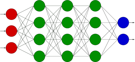
We arrange an artificial NN, see [3], to approximate the mapping (6). An NN consists of an input layer, an output layer and additional hidden layers. Figure 1 illustrates the schematic of an NN. Let $N_{j}$ be the number of neurons in the $j$th layer for $j=0,1,\ldots,J$. Therein, $j=0$ and $j=J$ represent the input layer and the output layer, respectively. Thus there are $J-1$ hidden layers. It holds that $N_{0}=q$ and $N_{J}=m$ and thus $N_{J}\gg N_{0}$ in our problem.

The mathematical model $\Psi:\mathbbm{R}^{N_{0}}\rightarrow\mathbbm{R}^{N_{J}}$ of an NN consists in a chain of operators

$$\Psi={T}_{J}\circ\rho\circ{T}_{J-1}\circ\rho\circ{T}_{J-2}\circ\cdots\circ\rho\circ{T}_{2}\circ\rho\circ{T}_{1}.$$ (7)

Each operator ${T}_{j}:\mathbbm{R}^{N_{j-1}}\rightarrow\mathbbm{R}^{N_{j}}$ is an affine-linear function

$${T}_{j}({z})={A}_{j}{z}+{b}_{j}$$

including a matrix ${A}_{j}\in\mathbbm{R}^{N_{j}\times N_{j-1}}$, a vector ${b}_{j}\in\mathbbm{R}^{N_{j}}$, and the input ${z}\in\mathbbm{R}^{N_{j-1}}$. In the context of machine learning, the entries of ${A}_{j}$ and ${b}_{j}$ are denominated as weights and biases, respectively. The operator $\rho$ is a nonlinear transfer function $\rho:\mathbbm{R}\rightarrow\mathbbm{R}$ (also called activation function). Typical choices are, for example, the hyperbolic tangent sigmoid function

$$\rho(x)=\frac{2}{1+{\rm e}^{-2x}}-1$$ (8)

and the hard-limit function

$$\rho(x)=\left\{\begin{array}[]{ll}0&\;\;\mbox{for}\;x<0,\\ 1&\;\;\mbox{for}\;x\geq 0.\\ \end{array}\right.$$ (9)

In (7), the function $\rho$ is applied to vectors in each component separately.

Figure 1: Artificial NN with input layer (red), hidden layers (green), and output layer (blue).

In the fitting of an NN, the ideal is to minimise the distances $\Theta({p})-\Psi({p})$ for any ${p}\in\Pi$. The degrees of freedom are the weights and biases, i.e., $({A}_{j},{b}_{j})_{j=1}^{J}$. Since a nonlinear optimisation problem appears, iterative methods are required to obtain numerical solutions.

In practise, the fitting involves three sample sets for training, validation, and test:

$$\begin{array}[]{rl}\mathcal{S}_{\rm train}&=\{{p}_{1},\ldots,{p}_{k}\}\subset\Pi\\[2.15277pt] \mathcal{S}_{\rm valid}&=\{{q}_{1},\ldots,{q}_{k^{\prime}}\}\subset\Pi\\[2.15277pt] \mathcal{S}_{\rm test}&=\{{r}_{1},\ldots,{r}_{k^{\prime\prime}}\}\subset\Pi.\\ \end{array}$$ (10)

For example, random samples can be chosen, where a uniform probability distribution is assumed in the parameter domain $\Pi$. The minimisation is based on the differences $\Theta({p}_{i})-\Psi({p}_{i})$ for parameter tuples ${p}_{i}$ from the training set. The (vector-valued) differences are measured using the mean squared error or the mean absolute error. The error measure decreases monotone for the parameters in the training set due to the minimisation. The validation set is included to prevent an overfitting. If the error measure of the validation set increases, then the training is stopped and the best previous case is put out. The test set is not involved in the minimisation at all. Hence this set allows for an estimate of the quality of the trained NN.

5 Numerical Results for Test Example

All numerical computations were performed within the software MATLAB [8] using the Deep Learning Toolbox.

We investigate an electric circuit introduced in [1], which is illustrated by Fig. 2. This circuit performs a voltage doubling for specific choices of parameters and input voltage. A mathematical modelling yields a nonlinear system of DAEs (1) with $n=3$ equations for the three unknown node voltages presented in [1]:

$$\begin{array}[]{rcl}C_{1}\dot{x}_{1}&=&-\frac{x_{1}}{R_{2}}+F(-(x_{1}+x_{3}))\\ C_{2}\dot{x}_{2}&=&-\frac{1}{R_{1}}(x_{2}+x_{3}+u_{\rm in})\\ 0&=&-\frac{1}{R_{1}}(x_{2}+x_{3}+u_{\rm in})+F(-(x_{1}+x_{3}))-F(x_{3}).\\ \end{array}$$ (11)

The current-voltage relation of the diodes reads as $F(u)=\gamma(\exp(\delta u)-1)$. We use the constant parameters $\gamma=4.067\cdot 10^{-8}$ and $\delta=5.634\cdot 10^{-2}$ given in [6]. The differential index of the DAE system (11) is one. We choose the second node voltage as QoI (3).

Figure 2: Diagram of electric circuit.

We consider variations in four physical parameters: the two capacitances and the two resistances. The ranges $C_{j}\in[2\cdot 10^{-9},3\cdot 10^{-9}]$ for $j=1,2$, $R_{1}\in[10^{6},2\cdot 10^{6}]$, $R_{2}\in[10^{8},2\cdot 10^{8}]$ form the parameter domain $\Pi\subset\mathbbm{R}^{4}$.

As input voltage, we supply the harmonic oscillation

$$u_{\rm in}(t)=A\sin\left(\frac{2\pi}{T}\,t\right)$$

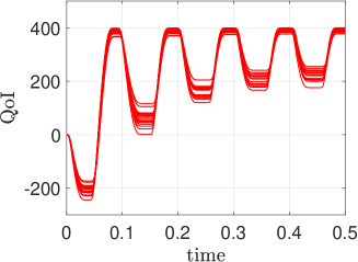
with amplitude $A=500$ and period $T=0.1$. The total time interval of our simulations is $[t_{0},t_{\rm f}]=[0,0.5]$. The initial values (2) are set to zero, which represents a consistent case in this example. The backward differentiation formulas (BDF), see [4], yield the numerical solutions of the IVPs. High accuracy requests are imposed in the local error control with relative tolerance $\varepsilon_{\rm rel}=10^{-4}$ and absolute tolerance $\varepsilon_{\rm abs}=10^{-6}$. The error control generates approximations on a non-uniform grid in time. We extract the trajectories of the QoI in $m=200$ equidistant time points $t_{\ell}=\ell\Delta t$ for $\ell=1,\ldots,m$ with $\Delta t=\frac{t_{\rm f}-t_{0}}{m}$ by interpolation. The order of accuracy coincides for both the uniform grid and non-uniform grid. The associated error of the time integration is negligible in comparison to the approximation error of the NNs below. Figure 3 gives an impression of the variability within the trajectories of the QoI for our parameter domain.

Figure 3: Twenty trajectories of the QoI for different parameter samples.

We select the number of samples as $k=k^{\prime}=k^{\prime\prime}=500$ in the sets (10). Often the validation set and the test set are chosen smaller than the training set due to a restricted amount of data. In contrast, we are able to use larger sets, since a high number of trajectories can be produced by numerical simulations. In particular, a large test set provides reliable statistics in the error analysis. A pseudo random number generator yields the parameter samples in the multidimensional cuboid $\Pi$. Our NNs include two hidden layers with 400 neurons in each layer. Using more hidden layers or more neurons did not improve the results significantly. We investigate two NNs, which differ only in the choice of the transfer function:

• hard-limit transfer function (9),

• purely linear transfer function.

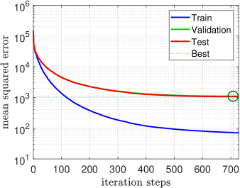
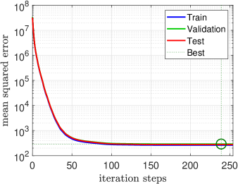
In the training, a conjugate gradient backpropagation method iteratively solves the minimisation problem. Figure 4 shows the performance of the training procedure. In the case of the hard-limit transfer function, the training is stopped at the 728th iteration step, because the error of the validation set increases slightly. In the case of the linear transfer function, the training is terminated at the 254th iteration step due to a too small step size. These two NNs are used in the following error analysis.

(i)                                                      (ii)

Figure 4: Mean squared errors during the fitting of the two NNs in the iterative minimisation. (The green line of the validation set is mostly located behind the red line of the test set.)

In addition, we tried two other backpropagation techniques in the training of the NNs: a one-step secant method (quasi Newton method) and a gradient descent method with momentum and adaptive learning rate. More information on all three methods can be found in [2], for example. Table 1 demonstrates the number of iteration steps (until a termination criterion applies) as well as the final mean squared error of the test set for the three techniques. We observe that the conjugate gradient method exhibits the best performance.

Table 1: Number of iteration steps and mean squared error (MSE) of test set for different training methods in NNs with hard-limit transfer function (i) and purely linear transfer function (ii).

	(i)		(ii)
	steps	MSE	steps	MSE
conjugate gradient method	728	1067.5	254	277.21
one-step secant method	1696	1062.2	328	277.24
gradient descent method	10000	1323.1	1413	277.74

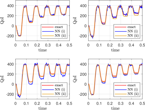
Figure 5 illustrates several trajectories of the test set. A comparison of the exact trajectories from the time integration and the approximations from the two NNs is shown. An interesting property is that NN (i) with the nonlinear transfer function exhibits an oscillatory behaviour of the approximations in time, whereas NN (ii) with the linear transfer function generates more smooth approximations in time. The incorrect behaviour is not a transient effect, because all discrete time points (5) are treated equally in the NNs, i.e., without the consideration of their ordering in time. We also tried other nonlinear transfer functions (like (8)), which still caused oscillations in time.

Figure 5: Trajectories of the QoI for some samples from the test set.

Finally, we quantify the relative errors of the approximations for each sample trajectory using a discrete $\mathcal{L}^{1}$-norm in time. The error associated to the $i$th parameter sample reads as

$$E_{i}=\frac{t_{\rm f}-t_{0}}{m}\sum_{\ell=1}^{m}\frac{\left|\tilde{y}(t_{\ell},{p}_{i})-y(t_{\ell},{p}_{i})\right|}{|y(t_{\ell},{p}_{i})|},$$ (12)

where $y$ is the original value from the time integration and $\tilde{y}$ denotes the approximation from an NN. The initial value is not included due to its value zero. The statistics of the errors are depicted in Table 2. We discuss the resulting mean values. In NN (i), a smaller mean error is achieved in the training set, whereas the other two sets show larger errors in comparison to NN (ii). Moreover, the mean errors are balanced for all three sets in NN (ii). This behaviour is in agreement to the performance of the training demonstrated by Fig. 4.

Table 2: Mean value and standard deviation of relative errors in discrete $\mathcal{L}^{1}$-norm, see (12), for the three parameter sets within the two trained NNs.

		NN (i)		NN (ii)
mean	training set	0.044		0.086
	validation set	0.130		0.086
	test set	0.120		0.079

		NN (i)		NN (ii)
st.dev.	training set	0.135		0.228
	validation set	0.210		0.158
	test set	0.155		0.146

6 Conclusions

We arranged a mapping from a set of parameters to discrete values of a QoI obtained from IVPs of dynamical systems. We approximated this mapping by artificial NNs. A test example was investigated, where two NNs were trained. In both NNs, the quality of the approximations is moderate with respect to the mean values of the errors. However, the NN including a linear transfer function yielded more smooth discretised trajectories in time, whereas the NNs with nonlinear transfer functions produced incorrect oscillations in time.

References

- [1] Barz, B., Suschke, E.: Numerische Behandlung eines Algebro-Differentialgleichungssystems. RZ-Mitteilungen, 7, Humboldt-Universität, Berlin (1994)
- [2] Du, K.-L., Swamy, M.N.S.: Neural Networks and Statistical Learning. Springer, London (2014)
- [3] Goodfellow, I., Bengio, Y., Courville, A.: Deep Learning. MIT Press (2017)
- [4] Hairer, E., Nørsett, S.P., Wanner, G.: Solving Ordinary Differential Equations I: Nonstiff Problems. (2nd ed.) Springer, Berlin (1993)
- [5] Hairer, E., Wanner, G.: Solving Ordinary Differential Equations II: Stiff and Differential-Algebraic Equations. (2nd ed.) Springer, Berlin (1996)
- [6] Kampowsky, W., Rentrop, P., Schmidt, W.: Classification and numerical solution of electric circuits. Surv. Math. Ind., 2, 23–65 (1992)
- [7] Le Maître, O.P., Knio, O.M.: Spectral Methods for Uncertainty Quantification. Springer, Dordrecht (2010)
- [8] MATLAB, version 9.7.0.1190202 (R2019b), The Mathworks Inc., Natick, Massachusetts (2019)
- [9] Pulch, R.: Polynomial chaos for the computation of failure probabilities in periodic problems. In: Roos, J., Costa, L. (eds.) Scientific Computing in Electrical Engineering SCEE 2008, Mathematics in Industry, vol. 14, pp. 191–198, Springer, Berlin (2010)
- [10] Sullivan, T.J.: Introduction to Uncertainty Quantification. Springer, Cham (2015)
- [11] Wang, Q., Hesthaven, J.S., Ray, D.: Non-intrusive reduced order modeling of unsteady flows using artificial neural networks with application to a combustion problem. J. Comput. Phys., 384, 289–307 (2019)
- [12] Yu, J., Hesthaven, J.S.: Flowfield reconstruction method using artificial neural network. AIAAJ, 57 (2019)